Happy Cruise Line Sediment Management Proposal and Air Pollution Impact Study

in Long Beach, CA

6/9/2014

Michigan State University College of Engineering

Daniel Domino (Design Engineer), Eunsang Lee (Lead Researcher), Steven C. McConnell

(Environmental Policy Expert), Priyank Patel (Modeling Engineer)

Photo credit: Aerial above Queen Mary and Carnival cruise ships Paradise vessel Long Beach harbor,

California, Arial Archives.com

Introduction and problem statement

Happy Cruise Line has proposed the dredging of contaminated sediment in order to build

a new docking facility in Long Beach, California. This sediment is contaminated with DDT and

PCB at concentrations of 80 ng/g and 50 ng/g, respectively, with hotspots that have

concentrations 10 times this amount. In order to obtain permission from the City of Long Beach

to construct the docking facility, Happy Cruise Line must propose a feasible sediment

management strategy that properly manages the dredged sediment while minimizing air, water,

and noise pollution, and traffic congestion during both the dredging and cruise line operations.

Sediment Management Plan

The Port of Long Beach (POLB) and the Contaminated Sediment Task Force (CSTF,

2005) (Figure 1) consider the use of contaminated sediment as port fill in a near shore confined

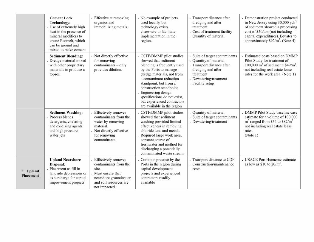
disposal facility (CDF) as the best sediment management strategy (Table 1). As such, the MSU

Team recommends the dredging and containment of the contaminated sediments in a CDF

(Figure 2), thereby incorporating this material for beneficial use the planned cruise ship pier. The

first step in the CDF construction process will be testing and geotechnical characterization of the

sediment and determination of the CDF area. The actual construction of the CDF will begin with

the placement of dikes that will encompass the proposed CDF. Water will be pumped from

within the CDF into the ocean. The saturated contaminated sediment will then be dredged and

placed in the CDF. Next, after allowing the contaminated sediment to settle, the supernatent

above the contaminated sediment will be removed from the CDF into the ocean. Based on our

estimates of the concentrations of DDT and PCB in the sediment pore water (Appendix D), we

anticipate that this marine water will not exceed criteria set under the California Toxics Rule

(CTR) during this process (Table 2) (Chiou). In addition, best management practices will be

employed to reduce the re-suspension of sediment associated with dredging (Table 3). If

pollutant concentrations exceed the CTR, additional treatment of the water will be required

before discharge to the ocean. Finally, clean sediment and then pavement will placed on top of

the contaminated sediment to further confine the contaminated sediment.

Further analysis demonstrates that the average sediment contaminant concentrations for

PCB and DDT at the site are both less than the probable effect concentration set under the

Sediment Quality Guidelines (Wisconsin DNR) (Table 4). However, due to hotspots, removal of

the contaminated sediments is strongly advised and we recommend containment as the most

suitable, technically feasible, and economical option. Containment within a CDF has been

estimated to cost $10/m3, which is far less than other technologies (Table 1). In addition, the use

of the contaminated material in the construction of the pier further reduces construction costs

attributed to the purchase and transport of clean material from outside of the site. Finally, the use

of a CDF as a sediment management strategy results in significantly lower air emissions when

compared to other possible methods such as thermal destruction or transportation to a landfill.

The MSU Team will obtain the requisite permits before the dredging and the construction

of the CDF begins. We anticipate that up to 36 months may be required to obtain these permits.

Under Section 402 of the Clean Water Act (CWA), an issued permit is necessary for the

discharge of any pollutant during the dredging and CDF construction process. In order to obtain

this permit, we plan to monitor the concentration of the pollutants in the sediment and water

prior discharge to ensure that our operations comply with Sections 301, 302, 303, 306, and 307

of the CWA and a water quality certification (FWPCA 2002) can be awarded. The outlined

project and sampling results must meet the standards, set under Section 401 of the CWA, in

order to receive a water quality certification (CRWQCB 2012).

Processes that will release air pollution include dredging and construction of the near-

shore CDF. The pollutants that will be released are reactive organic gases (ROGs), CO, NOx,

SO2, PM2.5 and PM10. Both the dredging and building of the CDF will be sources for these

pollutants. Table 5 in the Appendix shows the mass of each pollutant released per day by the

dredging equipment. Air quality is regulated by California Ambient Air Quality Standards

(CAAQS) (Table 6) (LSA, 2013). Long Beach is currently non-attainment for ozone, lead, and

PM 2.5. A simple box model was used to estimate the concentration of the pollutants added to

the ambient air of Long Beach. Emission factors are taken from AP-42 Sec 3.3 (EPA, 1996). The

calculations show that the CAAQS will not be exceeded during this dredging process. Total

concentrations of each pollutant can be seen in Figure 3 and Table 7.

During the dredging process, the MSU team proposes that mitigation strategies be used to

reduce air pollution. We recommend the use of Clean Diesel Combustion, a technology that

achieves higher engine efficiency and reduces emissions, thereby allowing the dredge engines to

meet requisite Tier 3 emission standards. To further reduce emissions, and ensure worker safety,

we recommend that a diesel particulate filter (DPF) be installed on the dredge and tugboat. These

DPFs remove the soot and PM from emissions with a conversion efficiency that meets the

California Airborne Toxic Control Measure for Stationary CI Engines (DCL International, 2008).

PCBs and DDT, both persistent organic pollutants, are regulated globally by The

Stockholm Convention (2001). Quality of Life (QOL) standards are set for PCB in air (EPA,

2004) (Table 8). Our proposed technology also addresses pertinent occupational exposure limits

(OELs) as set by the Occupational Safety and Health Administration (OSHA), as well as

California’s OSHA program (Cal/OSHA) (OSHA, 2014) (Table 9). We predict that PCB and

DDT concentrations in the air will meet these standards during the dredging and construction

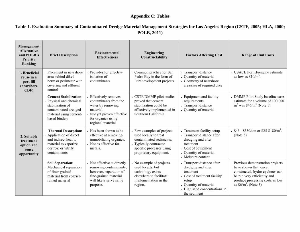
process. Monitoring can ensure these standards are met. Monitoring for PCBs and DDT involves

trapping these organic pollutants in polyurethane foam, and bringing these samples to a

laboratory for testing (EPA, 1999). Table 10 shows the detection limit of these pollutants and the

advantages and disadvantages of this sampling method (Figures 4 and 5).

Long-Term Management Plan

Potential sources that account for long term air pollution are additional traffic and cruise

ships. We estimated that the addition of the cruise line will add 1250 vehicles. A single cruise

ship produces exhaust equivalent to ~12,000 automobiles per day (Oceana, 2005). We suggest

that Happy Cruise Lines should collaborate with local bus companies who provide regular

service from Los Angeles to Long Beach to reduce traffic and air emissions.

In order to reduce the emission impact from ships, we recommend establishing an

Emission Control Area, which would require cleaner bunker fuel, reduced speed limits as cruise

ships approach ports, and cold ironing (turning off all engines while in port and plugging into

shore-side power).

The ground level concentration of the pollutants from additional cars was determined using a line

source model. Emission factors were taken from EPA (2008). According to line source model, the

maximum concentration of each pollutant was estimated near Highway 710, which is the main

route from the Los Angeles to the Long Beach port. Figures 6-10 show the concentration profile of

pollutants perpendicular to this route. Comparing the calculated maximum concentration of each

pollutant at 100 m from Highway 710 (Table 11), we concluded that adding approximately 1,250

cars is not likely to have a significant impact on the existing air quality in Long Beach.

Considering the aforementioned strategies, we believe the construction of a cruise port will be

feasible and sustainable, if a beneficial CDF management plan is implemented.

Special acknowledgments to:

Dr. Susan Masten

Scott McQuiston

Sue Pemberton

Environmental Engineering Student Society

Michigan State University, College of Engineering

WM-AWMA

EM-AWMA

CENTRAL AWMA

Appendix A: Acronyms and abbreviations

CAAQS-California Ambient Air Quality Standards

CWA-Clean Water Act

CDF-Confined disposal facility

CO-Carbon Monoxide

CSTF-Contaminated Sediment Task Force

DDT-Dichlorodiphenyltrichloroethane

DPF-Diesel particulate filter

ECA-Emission Control Area

NOx-Nitrogen Dioxides

OELs-Occupational exposure limits

OSHA-Occupational Safety and Health Administration

PM-Particulate matter

PCB-polychlorinated biphenyl

POLB-Port of Long Beach

QOL-Quality of Life Standards

ROG-Reactive Organic Gases

SOx-Sulfur Dioxides

Appendix B: Figures

Figure 1. Dredging Action Decision Tree (CSTF, 2005)

Figure 2. Confined Disposal Facility (American Association of Port Authorities, 2012)

Figure 3. Concentration of Criteria Pollutants During the Dredging Process Based on Box

Model

0

100

200

300

400

500

600

Co

nce

ntr

atio

n (

µg/

m3)

Pollutants

Concentration of criteria pollutants in Long Beach CA. (Short Term)

PM10

PM2.5

NO2

SO2

CO

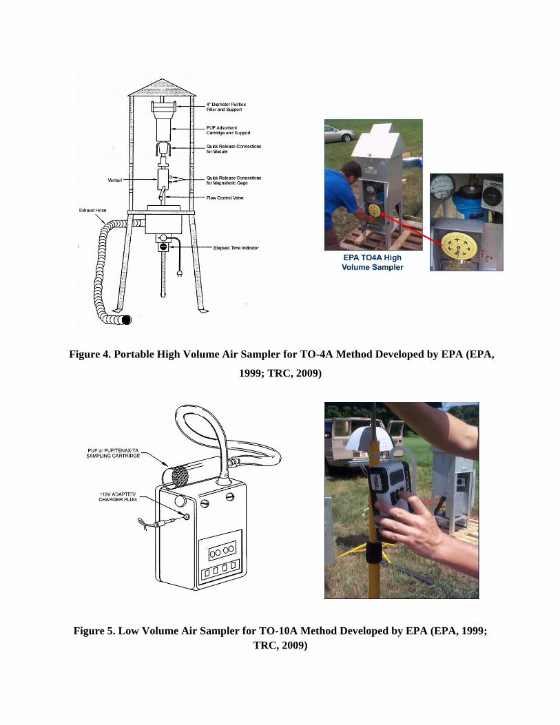
Figure 4. Portable High Volume Air Sampler for TO-4A Method Developed by EPA (EPA,

1999; TRC, 2009)

Figure 5. Low Volume Air Sampler for TO-10A Method Developed by EPA (EPA, 1999;

TRC, 2009)

Figure 6. PM10 Concentration Perpendicular to Highway 710 Based on Line Source Model

Figure 7. PM2.5 Concentration Perpendicular to Highway 710 Based on Line Source Model

0

0.05

0.1

0.15

0.2

0.25

0.3

0.35

0 0.5 1 1.5 2 2.5 3 3.5 4 4.5 5

Co

nce

ntr

atio

n (

µg/

m3

)

Distance (km)

PM10

0

0.005

0.01

0.015

0.02

0.025

0.03

0.035

0 0.5 1 1.5 2 2.5 3 3.5 4 4.5 5

Co

nce

ntr

atio

n (

µg/

m3

)

Distance (km)

PM2.5

Figure 8. Carbon Monoxide (CO) Concentration Perpendicular to Highway 710 Based on

Line Source Model

Figure 9. Nitrogen Oxides (NOx) Concentration Perpendicular to Highway 710 Based on

Line Source Model

0

10

20

30

40

50

60

70

0 0.5 1 1.5 2 2.5 3 3.5 4 4.5 5

Co

nce

ntr

atio

n (

µg/

m3

)

Distance (km)

CO

0

1

2

3

4

5

0 0.5 1 1.5 2 2.5 3 3.5 4 4.5 5

Co

nce

ntr

atio

n (

µg/

m3

)

Distance (km)

NOx

Figure 10. Volatile Organic Compounds (VOCs) Concentration Perpendicular to Highway

710 based on Line Source Model

0

1

2

3

4

5

6

7

0 0.5 1 1.5 2 2.5 3 3.5 4 4.5 5

Co

nce

ntr

atio

n (µ

g/m

3)

Distance (km)

VOC

Appendix C: Tables

Table 1. Evaluation Summary of Contaminated Dredge Material Management Strategies for Los Angeles Region (CSTF, 2005; HLA, 2000;

POLB, 2011)

Management

Alternative

and POLB’s

Priority

Ranking

Brief Description Environmental

Effectiveness

Engineering

Constructability Factors Affecting Cost Range of Unit Costs

1. Beneficial

reuse in a

port fill

(nearshore

CDF)

Placement in nearshore

area behind diked

berm or perimeter with

covering and effluent

control

Provides for effective

isolation of

contaminants.

Common practice for San

Pedro Bay in the form of

Port development projects.

Transport distance

Quantity of material

Geometry of nearshore

area/size of required dike

USACE Port Hueneme estimate

as low as $10/m3.

2. Suitable

treatment

option and

reuse

opportunity

Cement Stabilization: Physical and chemical

stabilization of

contaminated dredged

material using cement‐based binders

Effectively removes

contaminants from the

water by removing

material.

Not yet proven effective

for organics using

regional material

CSTF/DMMP pilot studies

proved that cement

stabilization could be

effectively implemented in

Southern California.

Equipment and facility

requirements

Transport distance

Quantity of material

DMMP Pilot Study baseline case

estimate for a volume of 100,000

m3 was $46/m

3 (Note 1)

Thermal Desorption:

Application of direct

and indirect heat to

material to vaporize,

destroy, or vitrify

contaminants

Has been shown to be

effective at removing/

immobilizing organics.

Not as effective for

metals.

Few examples of projects

used locally to treat

contaminated sediments.

Typically contractor

specific processes using

proprietary equipment.

Treatment facility setup

Transport distance after

dredging and after

treatment

Cost of equipment

Quantity of material

Moisture content

$45 - $330/ton or $25-$180/m3.

(Note 3)

Soil Separation: Mechanical separation

of finer‐grained

material from coarser‐rained material

Not effective at directly

removing contaminants;

however, separation of

fine-grained material

will likely serve same

purpose.

No example of projects

used locally, but

technology exists

elsewhere to facilitate

implementation in the

region.

Transport distance after

dredging and after

treatment

Cost of treatment facility

setup

Quantity of material

High sand concentrations in

the sediment

Previous demonstration projects

have shown that, once

constructed, hydro cyclones can

be run very efficiently and

produce processing costs as low

as $6/m3. (Note 5)

Cement Lock

Technology: Use of extremely high

heat in the presence of

mineral modifiers to

create Ecomelt, which

can be ground and

mixed to make cement

Effective at removing

organics and

immobilizing metals.

No example of projects

used locally, but

technology exists

elsewhere to facilitate

implementation in the

region.

Transport distance after

dredging and after

treatment

Cost of treatment facility

Quantity of material

Demonstration project conducted

in New Jersey using 30,000 yds3

of sediment showed a processing

cost of $50/ton (not including

capital expenditures). Equates to

approximately $92/m3. (Note 4)

Sediment Blending: Dredge material mixed

with other proprietary

materials to produce a

topsoil

Not directly effective

for removing

contaminants – only

provides dilution.

CSTF/DMMP pilot studies

showed that sediment

blending is frequently used

by the Ports to manage

dredge materials, not from

a contaminant reduction

standpoint, but from a

construction standpoint.

Engineering design

specifications do not exist,

but experienced contractors

are available in the region

Suite of target contaminants

Quantity of material

Transport distance after

dredging and after

treatment

Dewatering/treatment

Facility setup

Estimated costs based on DMMP

Pilot Study for treatment of

100,000 m3 of sediment: $49/m

3,

not including real estate lease

rates for the work area. (Note 1)

Sediment Washing: Process blends

detergents, chelating

and oxidizing agents,

and high pressure

water jets

Effectively removes

contaminants from the

water by removing

material.

Not directly effective

for removing

contaminants

CSTF/DMMP pilot studies

showed that sediment

washing provided limited

effectiveness in removing

chloride ions and metals.

Required large work area,

constant source of

freshwater and method for

discharging a potentially

contaminated waste stream.

Quantity of material

Suite of target contaminants

Dewatering/treatment

DMMP Pilot Study baseline case

estimate for a volume of 100,000

m3 ranged from $34 to $82/m

3

not including real estate lease

rates.

(Note 1)

3. Upland

Placement

Upland Nearshore

Disposal: Placement as fill in

landside depressions or

as surcharge for capital

improvement projects

Effectively removes

contaminants from the

site.

Must ensure that

nearshore groundwater

and soil resources are

not impacted.

Common practice by the

Ports in the region during

capital development

projects and experienced

contractors readily

available

Transport distance to CDF

Construction/maintenance

costs

USACE Port Hueneme estimate

as low as $10 to 20/m3.

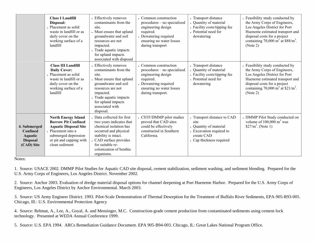
Notes:

1. Source: USACE 2002. DMMP Pilot Studies for Aquatic CAD site disposal, cement stabilization, sediment washing, and sediment blending. Prepared for the

U.S. Army Corps of Engineers, Los Angeles District. November 2002.

2. Source: Anchor 2003. Evaluation of dredge material disposal options for channel deepening at Port Hueneme Harbor. Prepared for the U.S. Army Corps of

Engineers, Los Angeles District by Anchor Environmental. March 2003.

3. Source: US Army Engineer District. 1993. Pilot‐Scale Demonstration of Thermal Desorption for the Treatment of Buffalo River Sediments, EPA‐905‐R93‐005.

Chicago, Ill.: U.S. Environmental Protection Agency

4. Source: Rehmat, A., Lee, A., Goyal, A. and Mensinger, M.C. Construction‐grade cement production from contaminated sediments using cement‐lock

technology. Presented at WEDA Annual Conference 1999.

5. Source: U.S. EPA 1994. ARCs Remediation Guidance Document. EPA 905‐B94‐003. Chicago, IL: Great Lakes National Program Office.

Class I Landfill

Disposal: Placement as solid

waste in landfill or as

daily cover on the

working surface of a

landfill

Effectively removes

contaminants from the

site.

Must ensure that upland

groundwater and soil

resources are not

impacted.

Trade aquatic impacts

for upland impacts

associated with disposal

Common construction

procedures – no specialized

engineering design

required.

Dewatering required

ensuring no water losses

during transport

Transport distance

Quantity of material

Facility costs/tipping fee

Potential need for

dewatering

Feasibility study conducted by

the Army Corps of Engineers,

Los Angeles District for Port

Hueneme estimated transport and

disposal costs for a project

containing 70,000 m3 at $88/m

3.

(Note 2)

Class III Landfill

Daily Cover:

Placement as solid

waste in landfill or as

daily cover on the

working surface of a

landfill

Effectively removes

contaminants from the

site.

Must ensure that upland

groundwater and soil

resources are not

impacted.

Trade aquatic impacts

for upland impacts

associated with

disposal.

Common construction

procedures – no specialized

engineering design

required.

Dewatering required

ensuring no water losses

during transport.

Transport distance

Quantity of material

Facility costs/tipping fee

Potential need for

dewatering

Feasibility study conducted by

the Army Corps of Engineers,

Los Angeles District for Port

Hueneme estimated transport and

disposal costs for a project

containing 70,000 m3 at $21/m

3.

(Note 2)

4. Submerged

Confined

Aquatic

Disposal

(CAD) Site

North Energy Island

Borrow Pit Confined

Aquatic Disposal Site Placement into a

submerged depression

or pit and capping with

clean sediment

Data collected for first

two years indicates that

chemical isolation has

occurred and physical

stability is intact.

CAD surface provides

for suitable re-

colonization of benthic

organisms.

CSTF/DMMP pilot studies

proved that CAD sites

could be effectively

constructed in Southern

California.

Transport distance to CAD

site

Quantity of material

Excavation required to

create CAD

Cap thickness required

DMMP Pilot Study conducted on

volume of 100,000 m3 was

$27/m3. (Note 1)

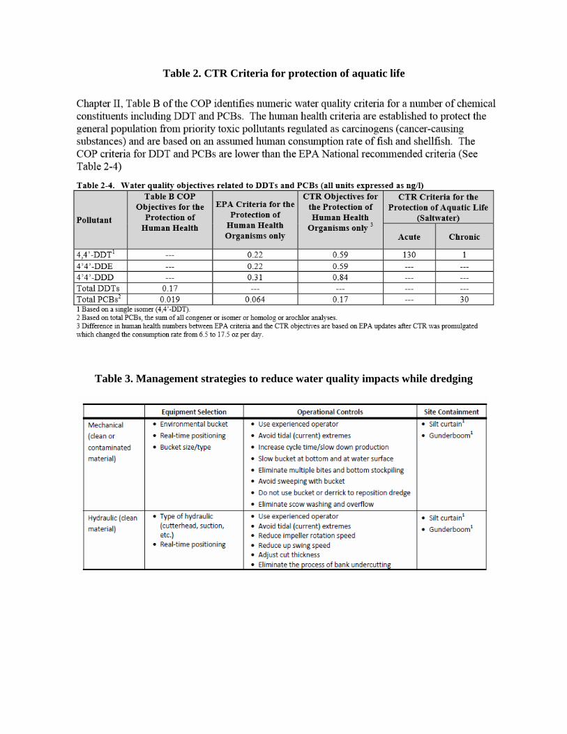
Table 2. CTR Criteria for protection of aquatic life

Table 3. Management strategies to reduce water quality impacts while dredging

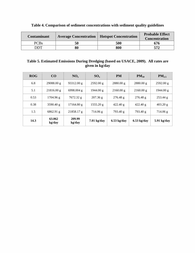
Table 4. Comparison of sediment concentrations with sediment quality guidelines

Contaminant Average Concentration Hotspot Concentration Probable Effect

Concentration

PCBs 50 500 676

DDT 80 800 572

Table 5. Estimated Emissions During Dredging (based on USACE, 2009). All rates are

given in kg/day

ROG CO NOx SOx PM PM10 PM2.5

6.8 29088.00 g 93312.00 g 2592.00 g 2880.00 g 2880.00 g 2592.00 g

5.1 21816.00 g 6998.004 g 1944.00 g 2160.00 g 2160.00 g 1944.00 g

0.53 1704.96 g 7672.32 g 207.36 g 276.48 g 276.48 g 253.44 g

0.38 3590.40 g 17164.80 g 1555.20 g 422.40 g 422.40 g 403.20 g

1.5 6862.91 g 21858.17 g 714.06 g 793.40 g 793.40 g 714.06 g

14.3 63.062

kg/day

209.99

kg/day 7.01 kg/day 6.53 kg/day 6.53 kg/day 5.91 kg/day

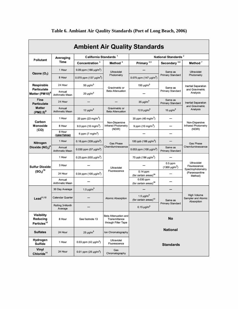
Table 6. Ambiant Air Qaulity Standards (Port of Long Beach, 2006)

Table 7. Dredging Process Emissions and Concentrations (based on USACE 2009)

Emissions

(kg/day)

Emission rate

(μg/m2·s)

C(8 hr)

(μg/m3)

Existing C(t)

(μg/m3)

Total C(t)

(μg/m3)

Standards

(μg/m3)

PM10 6.53 5.68 x 10-4

4.74 x 10-2

33.50 33.50 50

PM2.5 5.91 5.13 x 10-4

4.28 x 10-2

8.60 8.60 65

NO2 209.99 1.82 x 10-2

1.52 x 10-1

20.70 20.90 470

SO2 7.01 6.09 x 10-4

5.09 x 10-2

5.23 5.25 655

CO 63.06 5.48 x 10-3

4.57 x 10-2

573.7 574 10000

Table 8. Quality of Life Standards for PCBs (EPA, 2006)

Standard 24 hr average, total

PCBs

“Concern

Level”

Demonstration of

Compliance

Residential 0.11 g/m3 0.08 g/m

3

Continuous monitoring

24-hr samples Commercial/Industrial 0.26 g/m

3 0.21 g/m

3

Table 9. Cal/OSHA Regulatory Limits

Substance CAS NO.

Regulatory Limits Recommended Limits

OSHA

PEL

Cal/OSHA

(as of 4/26/13)

NIOSH REL

(as of 4/26/13)

ACGIH 2014

TLV

mg/m3

8-hour TWA

(ST) STEL

(C) ceiling

mg/m3

Up to 10-hour

TWA

(ST) STEL

(C) ceiling

mg/m3

8-hour TWA

(ST) STEL

(C) ceiling

mg/m3

Chlorodiphenyl

(42% Chlorine) 53469-21-9 1 1 0.001 1

Chlorodiphenyl

(54% Chlorine) 11097-69-1 0.5 0.5 0.001 0.5

Dichlorodiphenyltr

ichloroethane

(DDT)

50-29-3 1 1 0.5 1

Table 10. Summary of Sampling Methods for PCBs and DDT (EPA,1999)

Method

Types of

compounds

Determined

Sampling and Analysis Approach Detections

Limit Advantages Disadvantages

TO-4

Pesticides/PCBs

[e.g., PCBs, 4,4-

DDE, DDT and

DDD]

High vol. filter and PUF adsorbent

followed by GC/FID/ECD or

GC/MS detection

· Pesticides/PCBs trap on filter and

PUF adsorbent trap.

24 hr sampling

· Trap returned to lab, solvent

extracted and analyzed by

GC/FID/ECD or GC/MS

0.2 pg/m3

-

200 ng/m3

· Low detection Limits.

· Effective for broad range of

pesticides/PCBs.

· PUF reusable.

· Low blanks.

· Excellent collection and retention

efficiencies for common pesticides

and PCBs

· Breakdown of PUF adsorbent

may occur with polar extraction

solvents.

· Contamination of glassware

may limit detection limits.

· Loss of some semi-volatile

organics during storage.

· Extraneous organics may

interfere

· Difficulty in identifying

individual pesticides and PCBs

if using ECD.

TO-

10A

PUF adsorbent cartridge and

GC/ECD/PID/FID analysis

· A low-volume sample

· (1-5 L/min) is pulled through a

polyurethane foam (PUF) plug to

trap organochlorine pesticides.

24 hr sampling

· After sampling, the plug is

returned to the laboratory, extracted

and analyzed by GC coupled to

multi-metectors (ECD, PID,

· FID, etc.)

1-100

ng/m3

· Easy field use.

· Proven methodology.

· Easy to clean.

· Effective for broad range of

compounds.

· Portability.

· Good retention of compounds.

· ECD and other detectors

(except the MS) are subject to

responses from a variety of

compounds other than target

analysis.

· PCBs, dioxins and furans may

interfere.

· Certain orgagnocholorine

pesticides (e.g., chlordane) are

complex mixtures and can make

accurate quantitation difficult.

· May not be sensitive enough

for all target analytes in ambient

air.

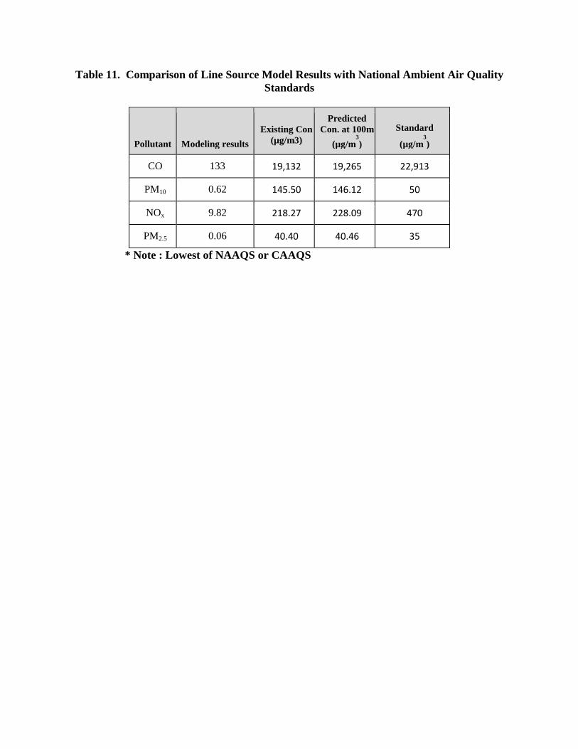
Table 11. Comparison of Line Source Model Results with National Ambient Air Quality

Standards

Pollutant Modeling results

Existing Con

(µg/m3)

Predicted

Con. at 100m

(µg/m3

)

Standard

(µg/m3

)

CO 133 19,132 19,265 22,913

PM10 0.62 145.50 146.12 50

NOx 9.82 218.27 228.09 470

PM2.5 0.06 40.40 40.46 35

* Note : Lowest of NAAQS or CAAQS

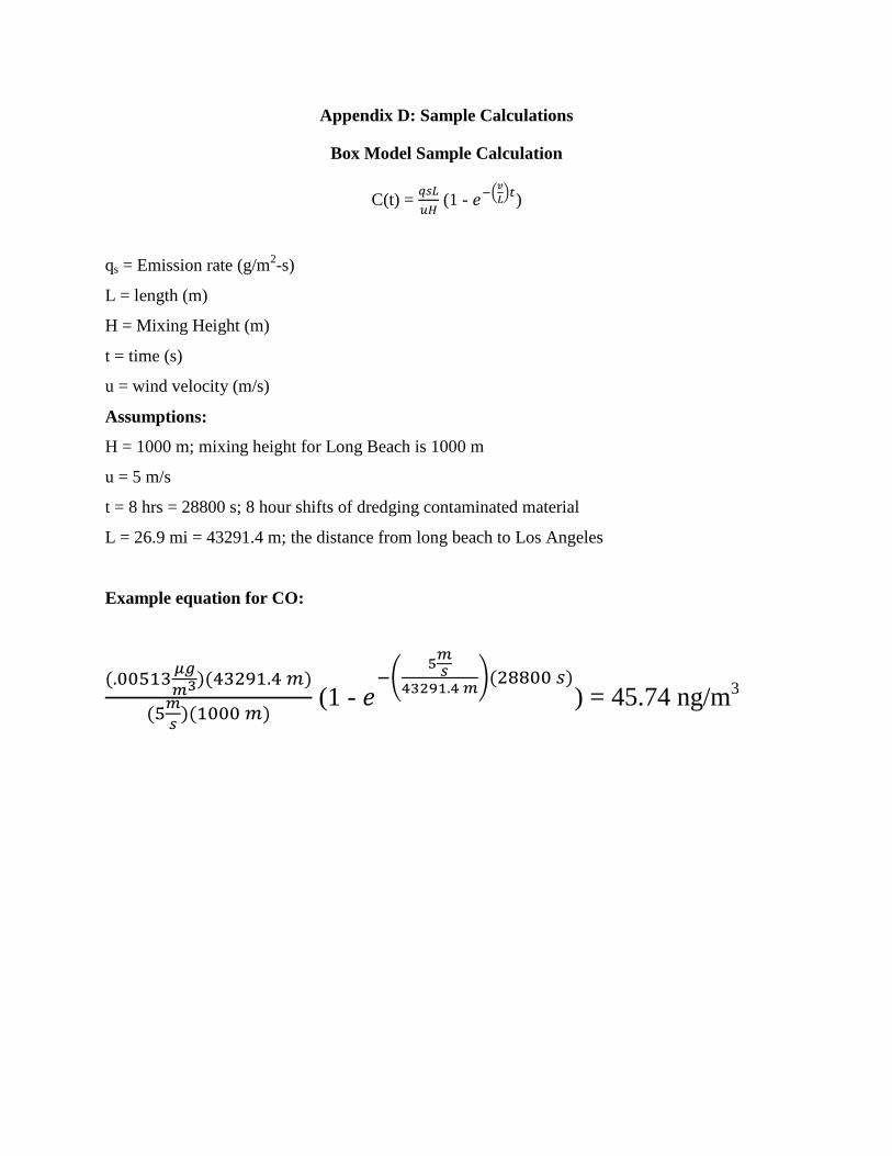
Appendix D: Sample Calculations

Box Model Sample Calculation

C(t) =

(1 - (

)

)

qs = Emission rate (g/m2-s)

L = length (m)

H = Mixing Height (m)

t = time (s)

u = wind velocity (m/s)

Assumptions:

H = 1000 m; mixing height for Long Beach is 1000 m

u = 5 m/s

t = 8 hrs = 28800 s; 8 hour shifts of dredging contaminated material

L = 26.9 mi = 43291.4 m; the distance from long beach to Los Angeles

Example equation for CO:

(1 - (

)

) = 45.74 ng/m3

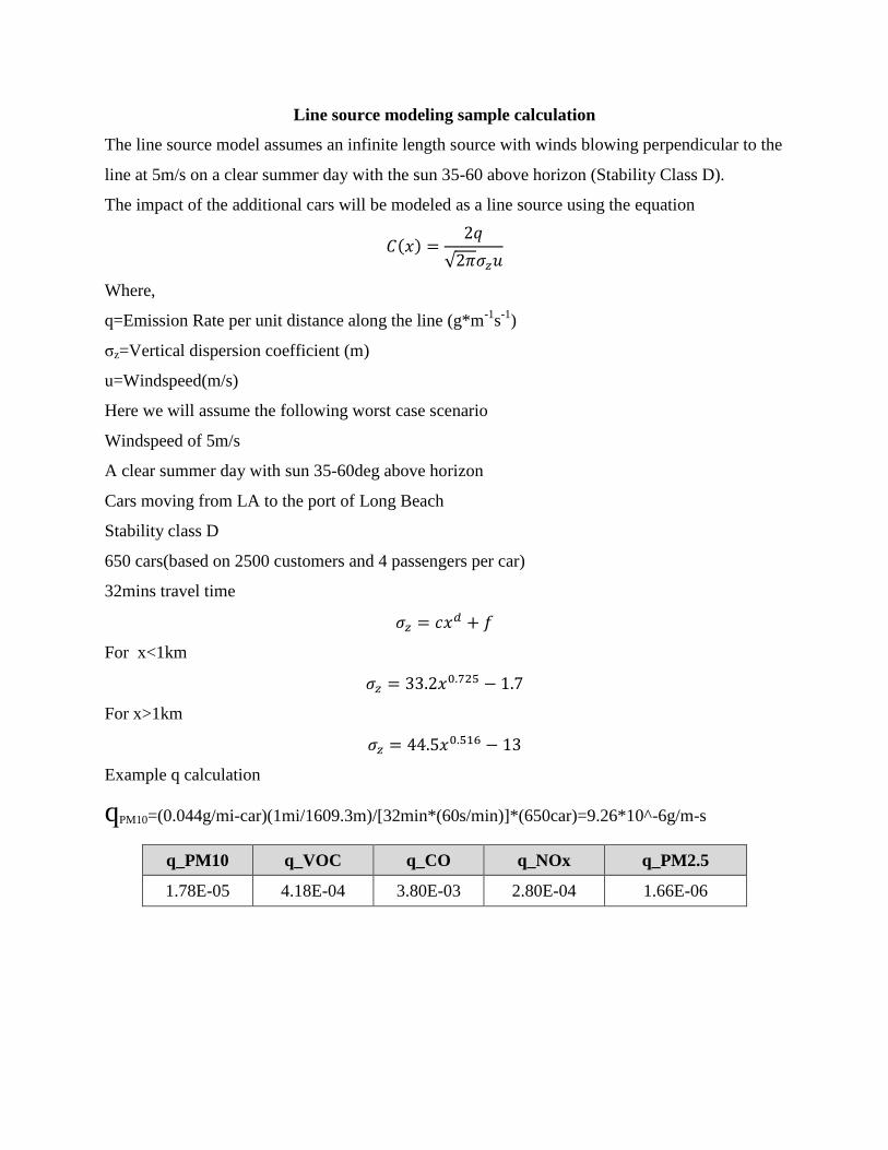
Line source modeling sample calculation

The line source model assumes an infinite length source with winds blowing perpendicular to the

line at 5m/s on a clear summer day with the sun 35-60 above horizon (Stability Class D).

The impact of the additional cars will be modeled as a line source using the equation

√

Where,

q=Emission Rate per unit distance along the line (g*m-1

s-1

)

σz=Vertical dispersion coefficient (m)

u=Windspeed(m/s)

Here we will assume the following worst case scenario

Windspeed of 5m/s

A clear summer day with sun 35-60deg above horizon

Cars moving from LA to the port of Long Beach

Stability class D

650 cars(based on 2500 customers and 4 passengers per car)

32mins travel time

For x<1km

For x>1km

Example q calculation

qPM10=(0.044g/mi-car)(1mi/1609.3m)/[32min*(60s/min)]*(650car)=9.26*10^-6g/m-s

q_PM10 q_VOC q_CO q_NOx q_PM2.5

1.78E-05 4.18E-04 3.80E-03 2.80E-04 1.66E-06

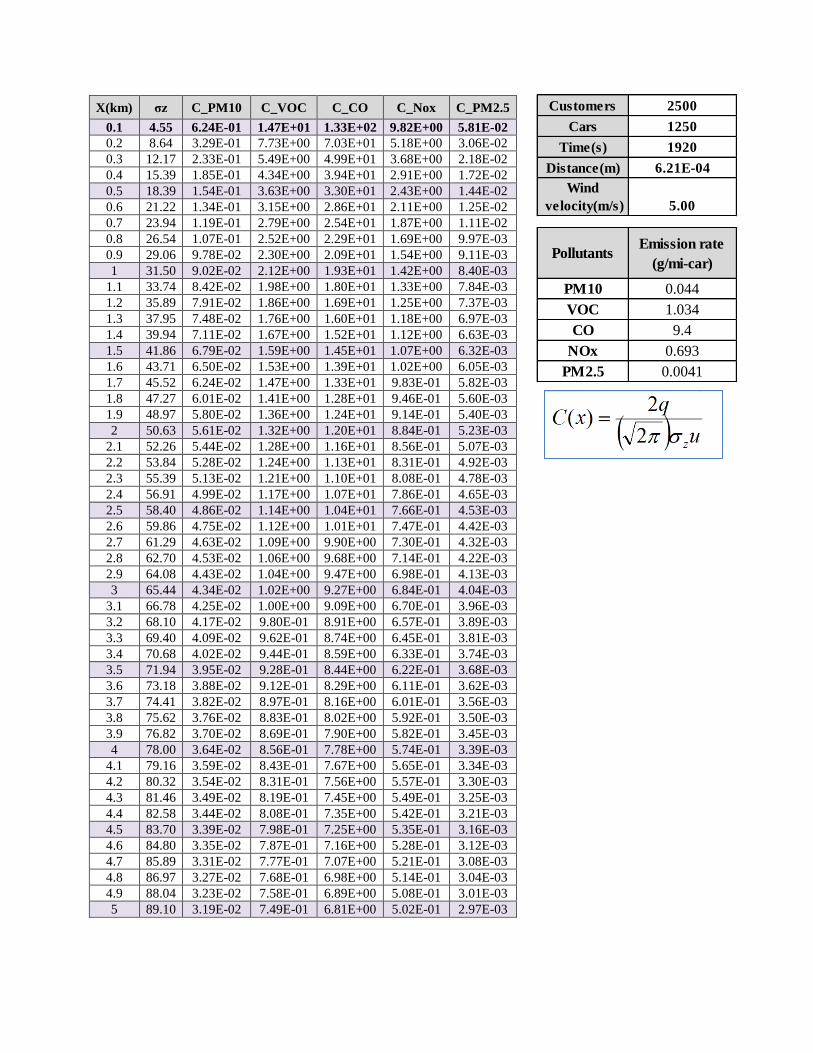
X(km) σz C_PM10 C_VOC C_CO C_Nox C_PM2.5

0.1 4.55 6.24E-01 1.47E+01 1.33E+02 9.82E+00 5.81E-02

0.2 8.64 3.29E-01 7.73E+00 7.03E+01 5.18E+00 3.06E-02

0.3 12.17 2.33E-01 5.49E+00 4.99E+01 3.68E+00 2.18E-02

0.4 15.39 1.85E-01 4.34E+00 3.94E+01 2.91E+00 1.72E-02

0.5 18.39 1.54E-01 3.63E+00 3.30E+01 2.43E+00 1.44E-02

0.6 21.22 1.34E-01 3.15E+00 2.86E+01 2.11E+00 1.25E-02

0.7 23.94 1.19E-01 2.79E+00 2.54E+01 1.87E+00 1.11E-02

0.8 26.54 1.07E-01 2.52E+00 2.29E+01 1.69E+00 9.97E-03

0.9 29.06 9.78E-02 2.30E+00 2.09E+01 1.54E+00 9.11E-03

1 31.50 9.02E-02 2.12E+00 1.93E+01 1.42E+00 8.40E-03

1.1 33.74 8.42E-02 1.98E+00 1.80E+01 1.33E+00 7.84E-03

1.2 35.89 7.91E-02 1.86E+00 1.69E+01 1.25E+00 7.37E-03

1.3 37.95 7.48E-02 1.76E+00 1.60E+01 1.18E+00 6.97E-03

1.4 39.94 7.11E-02 1.67E+00 1.52E+01 1.12E+00 6.63E-03

1.5 41.86 6.79E-02 1.59E+00 1.45E+01 1.07E+00 6.32E-03

1.6 43.71 6.50E-02 1.53E+00 1.39E+01 1.02E+00 6.05E-03

1.7 45.52 6.24E-02 1.47E+00 1.33E+01 9.83E-01 5.82E-03

1.8 47.27 6.01E-02 1.41E+00 1.28E+01 9.46E-01 5.60E-03

1.9 48.97 5.80E-02 1.36E+00 1.24E+01 9.14E-01 5.40E-03

2 50.63 5.61E-02 1.32E+00 1.20E+01 8.84E-01 5.23E-03

2.1 52.26 5.44E-02 1.28E+00 1.16E+01 8.56E-01 5.07E-03

2.2 53.84 5.28E-02 1.24E+00 1.13E+01 8.31E-01 4.92E-03

2.3 55.39 5.13E-02 1.21E+00 1.10E+01 8.08E-01 4.78E-03

2.4 56.91 4.99E-02 1.17E+00 1.07E+01 7.86E-01 4.65E-03

2.5 58.40 4.86E-02 1.14E+00 1.04E+01 7.66E-01 4.53E-03

2.6 59.86 4.75E-02 1.12E+00 1.01E+01 7.47E-01 4.42E-03

2.7 61.29 4.63E-02 1.09E+00 9.90E+00 7.30E-01 4.32E-03

2.8 62.70 4.53E-02 1.06E+00 9.68E+00 7.14E-01 4.22E-03

2.9 64.08 4.43E-02 1.04E+00 9.47E+00 6.98E-01 4.13E-03

3 65.44 4.34E-02 1.02E+00 9.27E+00 6.84E-01 4.04E-03

3.1 66.78 4.25E-02 1.00E+00 9.09E+00 6.70E-01 3.96E-03

3.2 68.10 4.17E-02 9.80E-01 8.91E+00 6.57E-01 3.89E-03

3.3 69.40 4.09E-02 9.62E-01 8.74E+00 6.45E-01 3.81E-03

3.4 70.68 4.02E-02 9.44E-01 8.59E+00 6.33E-01 3.74E-03

3.5 71.94 3.95E-02 9.28E-01 8.44E+00 6.22E-01 3.68E-03

3.6 73.18 3.88E-02 9.12E-01 8.29E+00 6.11E-01 3.62E-03

3.7 74.41 3.82E-02 8.97E-01 8.16E+00 6.01E-01 3.56E-03

3.8 75.62 3.76E-02 8.83E-01 8.02E+00 5.92E-01 3.50E-03

3.9 76.82 3.70E-02 8.69E-01 7.90E+00 5.82E-01 3.45E-03

4 78.00 3.64E-02 8.56E-01 7.78E+00 5.74E-01 3.39E-03

4.1 79.16 3.59E-02 8.43E-01 7.67E+00 5.65E-01 3.34E-03

4.2 80.32 3.54E-02 8.31E-01 7.56E+00 5.57E-01 3.30E-03

4.3 81.46 3.49E-02 8.19E-01 7.45E+00 5.49E-01 3.25E-03

4.4 82.58 3.44E-02 8.08E-01 7.35E+00 5.42E-01 3.21E-03

4.5 83.70 3.39E-02 7.98E-01 7.25E+00 5.35E-01 3.16E-03

4.6 84.80 3.35E-02 7.87E-01 7.16E+00 5.28E-01 3.12E-03

4.7 85.89 3.31E-02 7.77E-01 7.07E+00 5.21E-01 3.08E-03

4.8 86.97 3.27E-02 7.68E-01 6.98E+00 5.14E-01 3.04E-03

4.9 88.04 3.23E-02 7.58E-01 6.89E+00 5.08E-01 3.01E-03

5 89.10 3.19E-02 7.49E-01 6.81E+00 5.02E-01 2.97E-03

PollutantsEmission rate

(g/mi-car)

PM10 0.044

VOC 1.034

CO 9.4

NOx 0.693

PM2.5 0.0041

Customers 2500

Cars 1250

Time(s) 1920

Distance(m) 6.21E-04

Wind

velocity(m/s) 5.00

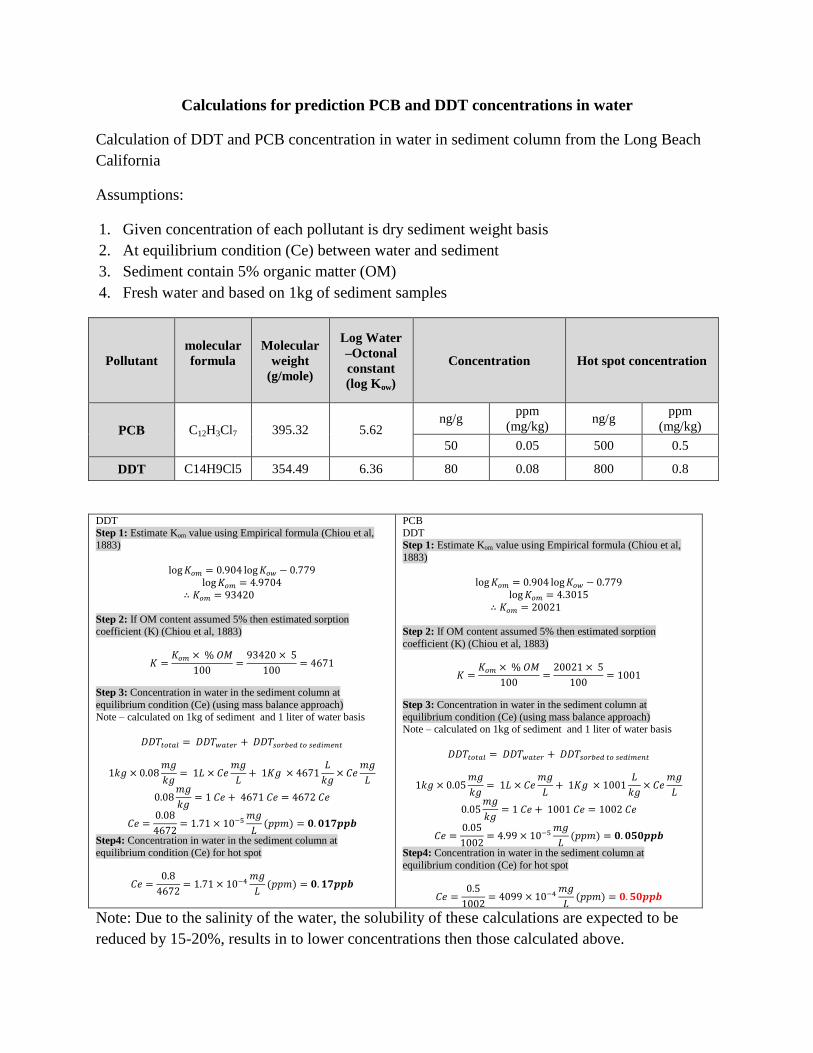
Calculations for prediction PCB and DDT concentrations in water

Calculation of DDT and PCB concentration in water in sediment column from the Long Beach

California

Assumptions:

1. Given concentration of each pollutant is dry sediment weight basis

2. At equilibrium condition (Ce) between water and sediment

3. Sediment contain 5% organic matter (OM)

4. Fresh water and based on 1kg of sediment samples

Pollutant

molecular

formula

Molecular

weight

(g/mole)

Log Water

–Octonal

constant

(log Kow)

Concentration Hot spot concentration

PCB C12H3Cl7 395.32 5.62 ng/g

ppm

(mg/kg) ng/g

ppm

(mg/kg)

50 0.05 500 0.5

DDT C14H9Cl5 354.49 6.36 80 0.08 800 0.8

DDT

Step 1: Estimate Kom value using Empirical formula (Chiou et al, 1883)

Step 2: If OM content assumed 5% then estimated sorption coefficient (K) (Chiou et al, 1883)

Step 3: Concentration in water in the sediment column at

equilibrium condition (Ce) (using mass balance approach)

Note – calculated on 1kg of sediment and 1 liter of water basis

Step4: Concentration in water in the sediment column at

equilibrium condition (Ce) for hot spot

PCB

DDT Step 1: Estimate Kom value using Empirical formula (Chiou et al,

1883)

Step 2: If OM content assumed 5% then estimated sorption

coefficient (K) (Chiou et al, 1883)

Step 3: Concentration in water in the sediment column at

equilibrium condition (Ce) (using mass balance approach) Note – calculated on 1kg of sediment and 1 liter of water basis

Step4: Concentration in water in the sediment column at

equilibrium condition (Ce) for hot spot

Note: Due to the salinity of the water, the solubility of these calculations are expected to be

reduced by 15-20%, results in to lower concentrations then those calculated above.

References

American Association of Port Authorities. “Beneficial Reuse of Dredge Materials at the Port of

Los Angeles” (2012). <http://www.aapa-

ports.org/files/SeminarPresentations/2012Seminars/12HNE/Walsh,%20David.pdf> accessed

6/8/2014

California Regional Water Quality Control Board Los Angeles Region (CRWQCB), (2012),

<http://www.waterboards.ca.gov/rwqcb4/water_issues/programs/401_water_quality_certi

fication/final_letters/Documents/2012/march/11-

192%20Shoreline%20Marina%20Fuel.pdf>

CSTF, “Los Angeles Regional Contaminated Sediments Task Force, Long-Term Management

Strategy, (2005). <http://www.coastal.ca.gov/sediment/long-term-mgmt-strategy-5-

2005.pdf> accessed 4/26/2014

EPA. “Ambient Air Monitoring Program”, (2013),

<http://www.epa.gov/oar/oaqps/qa/monprog.html> accessed 4/27/2014

EPA. “Ambient Air Monitoring Strategy for State, Local, and Tribal Air Agencies” (2008),

<http://www.epa.gov/ttn/amtic/files/ambient/monitorstrat/AAMS%20for%20SLTs%20%

20-%20FINAL%20Dec%202008.pdf> accessed 4/26/2014

EPA. “AP-42 section 3.3 Gasoline and Diesel Industrial Engines” (1996)

<http://www.epa.gov/ttnchie1/ap42/ch03/final/c03s03.pdf> accessed 4/26/2014

EPA. “Average Annual Emissions and Fuel Consumption for Gasoline-Fueled Passenger Cars

and Light Trucks” (2008). <http://www.epa.gov/otaq/consumer/420f08024.pdf> accessed

4/26/2014

EPA. “Compendium of Methods for the Determination of Toxic Organic Compounds in

Ambient Air - Second Edition” (1999).

<http://www.epa.gov/ttnamti1/files/ambient/airtox/tocomp99.pdf> accessed 4/26/2014

EPA. “Determination of Pesticides and Polychlorinated Biphenyls in Ambient Air Using Low

Volume Polyurethane Foam (PUF) Sampling Followed By Gas Chromatographic/Multi-

Detector Detection (GC/MD)” (1999), <

http://www.epa.gov/ttnamti1/files/ambient/airtox/to-10ar.pdf> accessed 6/8/2014

EPA. “Determination of Pesticides and Polychlorinated Biphenyls in Ambient Air Using High

Volume Polyurethane Foam (PUF) Sampling Followed by Gas Chromatographic/Multi-

Detector Detection (GC/MD)” (1999),

<http://www.epa.gov/ttnamti1/files/ambient/airtox/to-4ar2r.pdf > accessed 6/8/2014

EPA. “Hudson River PCBs Superfund Site Quality of Life Performance Standards” (2004).

<http://www.epa.gov/hudson/quality_of_life_06_04/full_report.pdf> accessed 4/25/2014

ERDC. “Liner Design Guidance for Confined Disposal Facility Leachate Control” (2004).

< http://el.erdc.usace.army.mil/elpubs/pdf/doerr6.pdf> accessed 4/27/2014

Federal Water Pollution Control Act (FWPCA), (2002), http://www.epw.senate.gov/water.pdf

Harding Lawson Associates (HLA). “The Beneficial Reuse of Dredged Material for Upland

Disposal” (2000)

LSA Associates. “Air Quality Impact Analysis” (2013).

<http://www.lbds.info/civica/filebank/blobdload.asp?BlobID=4156> accessed 4/25/2014

Oceana. “Needless Cruise Pollution” (2005)

<http://oceana.org/sites/default/files/o/fileadmin/oceana/uploads/cruise_pollution/polling

_report.pdf> accessed 4/26/2014

OSHA, “OSHA Annotated Table Z-1” (2014). <https://www.osha.gov/dsg/annotated-

pels/tablez-1.html accessed 4/26/2014> accessed 4/26/2014

Port of Long Beach, “Ambient Air Quality Standards” (2006),

<http://www.polb.com/civica/filebank/blobdload.asp?BlobID=3313> accessed 4/27/2014

Port of Long Beach. “Sediment Management Handbook for Dredge and fill projects” (2011)

Stockholm Convention on Persistent Organic Pollutants, (2001),

<http://chm.pops.int/Portals/0/Repository/convention_text/UNEP-POPS-COP-

CONVTEXT-FULL.English.PDF> accessed 4/26/2014.

TRC Corporation. “PCBs in Ambient Air Method Evaluation and Background Monitoring The

Hudson River, NY Sediment Remediation Project” (2009)

USACE. “Port of Los Angeles Channel Deepening Project Final SEIS/SEIR” (2009), <

http://www.portoflosangeles.org/EIR/ChanDeep/FEIR/3.2%20AirQuality%20Mar%2026

_jks.pdf> accessed 4/27/2014

Waymer, Kim.“Ships’ Soot Deadly, Study Shows.” Florida Today, Nov. 17 2007,

<pqasb.pqarchiver.com/floridatoday/access/1719620611.html?FMT=ABS&amp;date=No

v+17,+2007> accessed 4/24/2014

Wisconsin Dept. of Natural Resources. “Consensus-Based Sediment Quality Guidelines” (2003)