arX

iv:1

302.

1209

v2 [

mat

h.N

A]

24

Mar

201

3

Efficient pseudo-spectral solvers for the PKN model of

hydrofracturing.

Michal Wrobel(2,1), Gennady Mishuris(1,2),(1) Institute of Mathematical and Physical Sciences, Aberystwyth University,

Ceredigion SY23 3BZ, Wales U.K.,(2) Eurotech Sp. z o.o.,

ul. Wojska Polskiego 3, 39-300 Mielec, Poland

July 9, 2018

Abstract

In the paper, a novel algorithm employing pseudo-spectral approach is developed for the PKNmo-

del of hydrofracturing. The respective solvers compute both the solution and its temporal derivative.

In comparison with conventional solvers, they demonstrate significant cost effectiveness in terms of

balance between the accuracy of computations and densities of the temporal and spatial meshes.

Various fluid flow regimes are considered.

1 Introduction and preliminary results

Hydraulic fracturing is a widely used method for stimulation of hydrocarbons reservoirs. This technologyhas been known and successfully applied for a few decades [14, 12, 6]. Recently it has been revived,due to economical reasons, as a basic technique for exploitation of unconventional deposits of oil andgas. The phenomenon of a fluid driven fracture propagating in a brittle medium is also present in manynatural processes (e.g. magma driven dykes – [31], subglacial drainage of water – [34]).

Throughout the years, starting from the pioneering works of Sneddon and Elliot [32], Khristianovicand Zheltov [14], Perkins and Kern [30], Geertsma and de Klerk [11], and Nordgren [26], various modelsof hydrofracturing have been formulated and used in applications. A broad review of the topic can befound in [15, 16, 21, 17]. Together with increasing complexity of the models describing this multhiphysicsprocess, the computational techniques have been continuously enhanced. A comprehensive survey onthe algorithms and numerical methods used in hydrofracturing simulation can be found in [4, 9].

Responding to the recent demand, an increasing stream of publications have appeared concerningadditional information on seismic events, shear stresses in the rock formation, multifracturing and othersand their implementation into the solvers [35, 25, 27, 8]. Also, a considerable effort has been made toimprove the existing algorithms by incorporating new efficient numerical techniques [18, 21, 28, 29].

The main computational challenges associated with the modelling of hydraulic fractures are: a)strong nonlinearity resulting from the coupling between the solid and fluid phases, b) singularity of thegradients of the physical fields near the crack tip, c) moving boundaries, d) degeneration of the governingequations at the crack tip, multiscaling and others.

To achieve the maximal possible efficiency of numerical simulations, the computational algorithmsshould be formulated in proper variables accounting for all the problem peculiarities [21]. As a result,they allow one to reduce the volume of processed data, which is especially important when dealing withcomplex geometries and/or multifracturing.

1

The analysis presented in this paper is devoted to the PKN model of hydrofracturing. This modelcontains all the peculiarities mentioned above, except for the non-local relation for the fluid-solid cou-pling. Although we restrict our interest only to a single fracture, the developed algorithms, thanks totheir robustness, can be successfully applied to model a system of cracks.

The numerical analysis of the problem should be backdated to Nordgren [26] who extended thePerkins and Kern model [30] to account for the fluid loss effect and fracture volume change. As a result,the crack length was determined as part of the solution. The author proposed a finite difference schemeto solve the problem, which is in fact equivalent to the finite volume (FV) method.

Further development of the PKN formulation was done by Kemp [13], who (a) implemented thespecific boundary condition at the moving crack tip into the FV scheme, (b) incorporated asymptoticbehaviour of the solution near the crack tip in a special tip element, (c) indirectly used the fourth powerof the crack opening (w4) as a new dependent variable, instead of the crack opening itself. For theearly-time asymptotic model Kemp proposed a power series solution, presenting its first four terms.

The recent paper by Kovalyshen and Detournay[15] has extended most of Kemp’s results, incorpo-rating all information on the PKN model available to date. They present various asymptotics, completeanalytical solution for an impermeable rock (directly extending the results from [13] from four leadingterms to an infinite series representation), FV algorithm with a special tip element and a numericalbenchmark for the Carter leak-off, linking the results to the scaling approach developed in [3, 7, 23, 24].

In [19]-[21], the PKN model was reformulated by Linkov to improve the efficiency and stability ofcomputations by (i) introducing proper dependent variables (cubed fracture opening, w3), (ii) utilizingthe speed equation and (iii) by imposing a modified boundary condition at a small distance behindthe crack tip (ε-regularisation). Additionally, the analytical solution for an impermeable rock wasevaluated for the new dependent variable in a form of rapidly converging series in [21]. Moreover, theauthor highlighted in [19] that numerical schemes exploiting a fixed position of the crack tip during theiterations may become ill-posed.

In [22] and [17] the ε-regularisation technique was further enhanced by (i) appropriate adaptation ofthe speed equation to the chosen numerical scheme and (ii) improved way of imposing of the regularizedboundary condition. A detailed discussion on various aspects of application of implicit and explicitnumerical schemes was provided.

In this paper we are presenting a novel algorithm based on the pseudo-spectral approach. Namely,we propose an efficient numerical algorithm to solve a specific self-similar problem and extend the resultsto the general (transient) formulation. Since, the integration schemes used in the algorithm incorporatethe exact boundary conditions at the crack tip, no regularization technique is necessary. The mostaccurate two points representation of the temporal derivative is used to guarantee an optimal algorithmperformance. Finally, two solvers are developed which show their robustness and stability. They bothdemonstrate high cost effectiveness in terms of the relationship between the volume of the processeddata and the accuracy of computations. Moreover, additionally to the crack opening and length, thetemporal derivative of the former and the crack tip velocity are automatically returned as componentsof the problem solution.

1.1 Problem formulation

Let us consider a symmetrical crack of length 2l situated in the plane x ∈ [−l, l]. The crack is fully filledby a Newtonian liquid injected at the middle point (x = 0) with a known rate q0(t). Note here, that thecrack length evolution, l = l(t), is the result of fluid flow inside the fracture. Due to the symmetry ofthe problem, one can restrict the analysis to the half of the crack x ∈ [0, l(t)].

The classic mathematical formulation of the PKN model of hydrofracturing was given in [26]. Belowwe present a system of equations constituting the model. The mass conservation principle is expressed

2

by the continuity equation:

∂w

∂t+∂q

∂x+ ql = 0, t ≥ t0, 0 ≤ x ≤ l(t), (1)

while the Poiseuille equation describes the flow in a narrow channel. In the case of a Newtonian fluid,it is written in the following form:

q = −1

Mw3 ∂p

∂x. (2)

Here w = w(t, x) stands for the crack opening, q = q(t, x) is the fluid flow rate, p = p(t, x) (p = pf − σ0,σ0 - confining stress) refers to the net fluid pressure. The constantM , involved in the Poiseuille equation,is computed as M = 12µ, where µ denotes the dynamic viscosity (see for example [1]). The functionql = ql(t, x) from (1) is the volumetric rate of fluid loss to formation in the direction perpendicular to thecrack surfaces per unit length of the fracture. This function is usually assumed to be given, but it maydepend on the solution itself as well. To account for various leak-off regimes, we accept the followingbehaviour of ql:

ql(t, x) = Ql(t)(l(t) − x)η, for x→ l(t), (3)

for some constant η ≥ −1/2. Note that the case η = −1/2 corresponds to the Carter law [5], whileη ≥ 1/3 guarantees that the leak-off vanishes near the crack tip as fast as the crack opening at least (seefor details [17]).

The group of fluid equations is to be supplemented by the relation describing deformation of the rockunder applied hydraulic pressure. In the case of the PKN model, a linear relationship between the netfluid pressure and crack opening is in use:

p = kw, (4)

where a known proportionality coefficient k = 2πh

E1−ν2 is found from the solution of a plane strain

elasticity problem [26] for an elliptical crack of height h. E and ν are the elasticity modulus andPoisson’s ratio, respectively.

The above equations are equipped with the boundary condition at a crack mouth (x = 0) determiningthe injection flux rate:

−k

M

[

w3 ∂w

∂x

]

x=0

= q0(t), (5)

and two boundary conditions at a crack tip:

w(t, l(t)) = 0, q(t, l(t)) = 0. (6)

In order to define the crack length, l(t), the global fluid balance equation is usually utilized (see forexample [4])

∫ l(t)

0

[w(t, x) − w(0, x)]dx −

∫ t

0

q0(t)dt+

∫ l(t)

0

∫ t

0

ql(t, x)dtdx = 0.

(7)

Finally, the initial conditions are assumed in the following way:

w(0, x) = 0, l(0) = 0. (8)

System (1) – (8) constitutes the classic formulation of the PKN problem. It was shown in [13] and[10] that the asymptotic behaviours of w and q near the crack tip are interrelated, and the first term ofthe expansion for the crack opening may be written as:

w(t, x) ∼ w0(t) (l(t)− x)α, as x→ l(t). (9)

3

For the classic PKN model the exponent α = 1/3 was found in [13]. Thus condition (6)2 is alwayssatisfied as it follows from (2) and (4). As a result, the model does not account for the standard stresssingularity of fracture mechanics at the crack tip, and thus is relevant for the so-called zero toughnessregime (see e.g.[1]).

Remark 1. Despite that zero crack opening and length are considered as the initial conditions,all authors begin their studies from the asymptotic model for the small time. With the assumption ofzero leak-off term in the continuity equation and constant q0, the problem is reduced to a self-similarformulation. The full numerical analysis is then continued by taking the similarity solution as the initialstate. This effectively means that the initial conditions (8) can be replaced by the non-zero crack opening

l(0) = l⋄, w(0, x) = w⋄(x), x ∈ (0, l⋄). (10)

In this paper, the modified formulation of the PKN model is considered, following the recent advancein the area of numerical modelling [19, 20, 21, 22]. Thus, to trace the fracture front we use the so-calledspeed equation, instead of the fluid balance relationship (7):

dl

dt= v0(t) =

q

w

∣

∣

x=l(t). (11)

The speed equation assumes that the fracture tip coincides with the fluid front, which excludes thepresence of a lag or an invasive zone ahead of the fracture tip. Originally it was introduced by Kemp[13] and has been recently revisited by Linkov [19, 20, 21].

Note that, on substitution of equations (2), (4) and (9) into (11), one obtains a relationship betweenthe crack propagation speed and the multiplier of the leading term of the crack opening asymptoticexpansion (9):

dl

dt=

k

3Mw3

0(t). (12)

This implies that the quality of the numerical estimation of w0 (see estimate (9)) should be vital for theaccuracy of computations.

By substituting the Poiseulle equation (2) into the continuity equation (1) one obtains a lubrica-tion (Reynolds) equation for the considered problem, where the net fluid pressure function p(t, x) iseliminated:

∂w

∂t−

k

M

∂

∂x

(

w3 ∂w

∂x

)

+ ql = 0, t ≥ t0, 0 ≤ x ≤ l(t). (13)

In this way the modified formulation of the PKN model includes: i) the Reynolds equation (13); ii)the boundary conditions (5) – (6)1; iii) the asymptotics (9); iv) the initial conditions (10); v) the speedequation in the form (12).

The paper is organized as follows: in the next subsection we present the normalized formulationof the problem. Then, two types of self-similar solutions for the PKN model are discussed. Thesesolutions are used in section 2 to investigate a numerical algorithm for a time independent variant of theproblem. In section 3, the algorithm is modified to tackle the transient regime. Two alternative integralsolvers are developed and their performances and applicability are examined. Section 4 contains thefinal conclusions.

1.2 Normalized formulation.

Following [17], we normalize the problem by introducing dimensionless variables:

x =x

l(t), t =

t

tn, tn =

M

kl⋄, w⋄(x) = w⋄(x),

4

w(t, x) =w(t, x)

l⋄, L(t) =

l(t)

l⋄, l2

⋄q0(t) = tnq0(t), (14)

l⋄ql(t, x) = tnql(t, x), l2/3⋄ w0(t)/L

1/3(t) = w0(t),

where x ∈ [0, 1], L(0) = 1.In the new variables equation (13) reads:

∂w

∂t− x

L′

L

∂w

∂x−

1

L2(t)

∂

∂x

(

w3 ∂w

∂x

)

+ ql = 0, (15)

t ≥ 0, 0 ≤ x ≤ 1.

The boundary conditions (5) – (6)1 may be rewritten as:

−1

L(t)

[

w3 ∂w

∂x

]

x=0

= q0(t), w(t, 1) = 0. (16)

The initial conditions (10) are defined as:

L(0) = 1, w(0, x) = w⋄(x), x ∈ [0, 1]. (17)

The asymptotic expansion for crack opening (9) takes the form:

w(t, x) ∼ w0(t)(1− x)1/3, for x→ 1. (18)

For the sake of completeness of the normalization, we also present the global fluid balance equation(7), although it will not be used later on:

L(t)

∫ 1

0

w(t, x)dx −

∫ 1

0

w(0, x)dx −

∫ t

0

q0(t)dt

+

∫ t

0

L(t)

∫ 1

0

ql(t, x)dxdt = 0.

(19)

Finally, the transformation of the speed equation (12) yields:

d

dtL(t) = V0(t) =

1

3L(t)w3

0(t). (20)

As shown in [22], equation (20) is convenient to trace the fracture front when standard ODE solversare in use for the dynamic system describing the problem. On the other hand, the crack length can becomputed from (20) by direct integration to give:

L(t) =

√

1 +2

3

∫ t

0

w30(τ)dτ , (21)

which is useful when an implicit method (for example Crank-Nicolson scheme) is utilised (see [22]).On substitution of (20) into (15) one can rewrite the later to obtain:

3L2

(

∂w

∂t+ ql(t, x)

)

= xw30

∂w

∂x+ 3

∂

∂x

(

w3 ∂w

∂x

)

. (22)

In the following, equation (22) will be used as a basic relation to formulate our integral solvers.From now on, for convenience, we shall omit the tilde symbol in all quantities. In this way all the

notations refer henceforth to the normalized formulation.

5

1.3 Self-similar solutions

Let us assumeql(t, x) = γeγtq∗l (x), (23)

and look for the similarity solution of the problem in the form:

w(t, x) = u(x)eγt, w0(t) = u0eγt, (24)

where the asymptotic behaviour (18) holds true, and u0 is the limiting value of u defined in the samemanner as in estimate (18). Thus, equation (20) transforms to an identity if one takes:

L2(t) =2u309γ

e3γt. (25)

On substitution of (23), (24), and (25) into the equation (22) one can reduce the latter to the followingordinary differential equation:

βu30(u+ q∗l ) = A(u), (26)

with β = 2/3. Here, the nonlinear differential operator A is defined by the right-hand side of equation(22) and is equipped with the boundary conditions

− 3u−3/20

[

u3du

dx

]

x=0

= q∗0 , u(1) = 0, (27)

where we have introduced an auxiliary notation:

q∗0 =

√

2

γe−

5γt

2 q0(t). (28)

If q∗0 is constant, then equation (26) together with the boundary conditions (27) do not depend on timeand constitute a boundary value problem (BVP) degenerated at point x = 1. Indeed, the nonlinearcoefficient in front of the second order term of the differential operator vanishes at the point x = 1 inview of the boundary condition (27)2. This BVP is in fact a self-similar formulation of the originalproblem with specific, given leak-off regime and the inlet flux.

Other class of similarity solutions can be found, for some a ≥ 0, by assuming:

ql(t, x) = γ(t+ a)γ−1q∗l (x), w(t, x) = (t+ a)γu(x),

w0(t) = u0(t+ a)γ , (29)

L2(t) =2u30

3(3γ + 1)(a+ t)3γ+1. (30)

As a result, one again obtains the BVP (26) – (27) with β = 2γ/(3γ + 1) and

q∗0 =

√

6

(3γ + 1)(a+ t)

1−5γ

2 q0(t). (31)

Thus, for γ = 1/5 the self-similar solution corresponds to the constant injection flux rate, while the crackpropagation speed decreases with time as L′(t) = O(t−1/5) for t → ∞. If, however, one takes γ = 1/3,the crack propagation speed is constant and the injection flux rate increases with time: q0(t) = O(t1/3)for t→ ∞.

6

Note that self-similar solutions do not necessarily satisfy the initial conditions (17) as the normalisedinitial crack lengths are:

L(0) =

√

2u309γ

, L(0) =

√

2u30a3γ+1

3(3γ + 1),

for the first and the second type, respectively.Remark 2. As one can see the second type of similarity solution has a physical sense for any

−1/3 < γ < ∞ and thus, can be used to model three different transient regimes of the crack evolution:crack acceleration (γ > 1/3), crack deceleration (γ < 1/3), and a steady-state propagation of the fracture(γ = 1/3). The first type of solution possesses a physical interpretation only for positive values of γ,which restricts its application to the cases of accelerating crack.

The self-similar solutions formulated above are used in the following sections to analyse computationalaccuracy provided by the developed solvers. So far to this end, the asymptotic models have been usuallyemployed [26, 13, 15, 21]. However, all of them are restricted to the case of a constant influx, q0.

2 Numerical solution of the self-similar problem

In this section we will formulate an algorithm of the solution for the self-similar problem defined byequation (26) and the boundary conditions (27). The following representation of the sought functionu(x) will be accepted:

u(x) = u0(1− x)1/3 +∆u(x). (32)

It results from the asymptotic behaviour (18) and ∆u(x) = O((1 − x)ζ) for x → 0. Parameter ζ > 1/3depends strongly on the behavior of the leak-off function ql near the crack tip. In particular, when qlvanishes near the crack tip in the same manner as the solution, or faster, (η ≥ 1/3) then ζ = 4/3. Onecan show that (compare (3))

ζ = min{4/3, 1 + η} ≥ 1/2, (33)

see also [17] for details.

2.1 Integral solver for the self-similar problem.

Below we present an algorithm to solve equation (26) by numerical inversion of the operatorA. Exploitingthe solution representation (32), the inverse operator A−1 defines both components: u0 and ∆u. Toderive A−1, we integrate the equation (26) twice over the interval [x, 1] taking into account the boundarycondition (27)2. Then, after simple transformations one obtains:

3u30(1 − x)∆u = − 34 [6u

20(1− x)2/3(∆u)2+

4u0(1 − x)1/3(∆u)3 + (∆u)4] + u30

∫ 1

x

∆udξ+

2u30

∫ 1

x

(ξ − x)udξ − (1 − x)u30

∫ 1

x

udξ+

βu30

∫ 1

x

(ξ − x)(u + q∗l )dξ.

(34)

In short, the latter can be symbolically written in the compact form:

∆u = G1(β, u0,∆u) +G2(β, u0,∆u, q∗

l ), (35)

7

where the operators involved in the right-hand side are defined as follows:

3u30(1 − x)G1 = − 34

[

6(u20(1 − x)2/3(∆u)2+

4u0(1 − x)1/3(∆u)3 + (∆u)4]

+

(2 + β)u30

∫ 1

x

(ξ − x)∆udξ,

(36)

3(1− x)G2 = x

∫ 1

x

∆udξ +3

28(3β − 1)u0(1 − x)7/3+

β

∫ 1

x

(ξ − x)q∗l dξ. (37)

One can conclude from (3) and (18) that for x→ 1

G1 = O(

(1− x)1+ζ)

, G2 = O(

(1− x)ζ)

, (38)

where ζ defined in (33).The relation to compute u0 is derived by integration of (26) with respect to x from 0 to 1. Then,

taking into account the representation (32) and the boundary condition (27)1, one can formulate thecondition:

G3(β, u0,∆u, q∗

0) = 0, (39)

where

G3 =3

4(β + 1)u

5/20 +

u3/20

[

(β + 1)

∫ 1

0

∆udx+ β

∫ 1

0

q∗l dx

]

− q∗0 .

It is easy to prove that for any q∗0 > 0 and β > −1 there exists a unique positive solution u0 of equation(39), regardless of the values of the functions ∆u and q∗l .

The inverse operator A−1 is defined, by equations (35) and (39), as:

[u0,∆u] = A−1(β, q∗l , q∗

0). (40)

Its numerical execution is based on the following iterative algorithm:

G3

(

β, u(i+1)0 ,∆u(i), q∗0

)

= 0,

∆u(i+1) = G1

(

β, u(i+1)0 ,∆u(i)

)

+

G2

(

β, u(i+1)0 ,∆u(i), q∗l

)

,

(41)

where superscripts refer to the consequent iterations. In the first step we assume that:

∆u(0) = 0. (42)

Of course, if any better approximation is available, it can replace (42). Note the first relation of (41) is anonlinear algebraic equation that can be solved e.g. by the Newton-Raphson method, while the secondequation is a typical iterative relationship.

8

2.2 Numerical examples and discussions

In this section we investigate the performance of the numerical algorithm (41) – (42). To this end,the power law type self-similar solution (29) is utilized as a benchmark. Apart from the fact that theequations for other self-similar solution (24) look identically, the value of the parameter β appearingin the exponential benchmark is always the same (β = 2/3). Thus the power law type self-similarbenchmark gives us an opportunity to manipulate with the value of β, which will be crucial for furtherimplementation of the algorithm to the transient regime.

Let us utilize the following variant of benchmark solution used previously in [22] (compare (63) inthe Appendix A):

u(x) = (1− x)1/3(1 + s(x)), (43)

s(x) = −1

8e

(

1

3−

2γ

3γ + 1

)

(1− x) + 0.05(1− x)2,

which yields η = 4/3.Computations are carried out for different meshes based on N + 1 nodal points:

x()j = 1−

(

1−j

N

)

, j = 0, 1, ..., N. (44)

When one sets = 1, the points of spatial mesh are uniformly distributed over the whole interval -this mesh will be called the uniform mesh. By taking > 1 we obtain increased mesh density whileapproaching the end point x = 1 (the larger the greater mesh density near the crack tip) - this meshwill be refereed to as the non-uniform mesh. In our computations we will use = 3. This choice ismotivated by the following reason. To increase the solution accuracy, we compute integral operatorsfrom (41) using the classic Simpson quadrature, which gives an error controlled by the fourth derivativeof the integrand. Accounting for the asymptotic behaviour of the solution, the transformation (44), for = 3, improves the smoothness of the integrand with respect to the new independent variable near thecrack tip (replaces the fraction powers function). In this way, the error of integration can be minimized.We shall confirm this below in numerical tests.We use two parameters as the measures of computational accuracy: (i) – the maximal point-wise relativeerror (denoted as: δu) of the complete solution u(x) and (ii) – a relative error (denoted by δu0) of thecoefficient u0 defining the leading asymptotic term in (32).

The efficiency of computations will be assessed by the number of iterations needed to compute thesolution. The iterative process is stopped in each case when the L2-norm of the relative differencebetween two consecutive approximations becomes smaller than ǫ = 10−10. Finally, we analyze how thesolution errors depend on the number of nodal points N .

The computations revealed that convergence of the iterative process (41) may only be achieved forsome range of β values. For the analyzed benchmark it was: β ∈ [−1.8, 4.8]. In fact, this interval iswider than one could expect and fully covers any physically motivated values of β ∈ (0, 2/3) followingfrom the self-similar formulation. Interestingly, there are also solutions for β < −1 (compare discussionsafter equation (39)). This information shall be used later on, to construct a solver for transient regimes.

In Fig. 1a) the values of δu and δu0 obtained for the analyzed benchmark (43) are shown. Thecomputations were done for the meshes composed of 100 nodes. As can be seen, the non-uniform meshgives at least one order better accuracy of the solution, for the same number of nodal points. The errorof u0 is lower than the error of the complete solution u(x), as one could expect, while its distributionis not as smooth as for δu(x). The minimum of δu(x) is located near β = 1/3 which corresponds tothe steady-state similarity solution. Interestingly, in the case of the uniform mesh the aforementionedminimum is deeper and sharper than for the non-uniform one.

Fig. 1b) depicts the number of iterations needed to obtain the final solution for different values ofβ. It shows that the convergence rate almost does not depend on the type of mesh chosen. The best

9

−1 0 1 2 3 4−1.8 4.8

10−10

10−8

10−6

10−4

β

δu0

δu

a)

−1 0 1 2 3 4−1.8 4.8

101

102

103

num

ber

ofit

eratio

ns

non-uniform mesh

uniform mesh

β

b)

Figure 1: a) The accuracy of computations: maximal relative error of u(x) and u0 as a function of β;b) Number of iterations to reach the final solution as a function of β. Dashed lines refer to the uniformmesh, solid lines to the non-uniform mesh (for = 3).

20 50 100 150 20010

−8

10−7

10−6

10−5

10−4

β = −1

β = 0

β = 1

N

a)

50 100 150 2002010

−10

10−9

10−8

10−7

10−6

10−5

β = −1

β = 0

β = 1

N

b)

Figure 2: The maximal relative error of solution as a function of the number of nodal points N : a) δu,b) δu0. Dashed lines refer to the uniform mesh, solid lines to the non-uniform mesh (for = 3).

efficiency of computations appears for approximately |β| < 1/2. Note that this interval corresponds tothe values of β which provide the best accuracy of computations. The time of computations (numberof iterations) increases with |β| growth, however this trend does not exhibit a bilateral symmetry (fornegative and positive values of β). Moreover, the cost of computations increases with the solution error.

Fig. 2 shows how the accuracy of computations depends on the number of nodal points N . Bothchosen meshes are analyzed for three different values of β = −1, 0, 1. It can be seen that the non-uniformmesh gives at least two orders of magnitude better accuracy than the regular one. For both types ofmeshes, the values of δu0 are much lower than respective δu, however the best result for δu0 does notnecessarily correspond to the best δu (e.g. β = −1 for the regular mesh). The non-uniform mesh

10

50 100 150 2002010

−8

10−7

10−6

10−5

= 1

= 2

= 3

= 4

= 5

N

δu

Figure 3: The maximal relative error of solution δu0 for various spatial meshes. Computations weredone for β = 1/3.

provides much lower sensitivity of solution accuracy to the variation of β than the uniform one. Alsothe maximal level of accuracy is obtained much faster for the non-uniform mesh. In the considered case,it is sufficient to take only 60 nodal points to achieve the maximal possible accuracy.

The last test in this subsection identifies the influence of spatial meshing on the solution accuracy.To this end, we consider the following values of = 1, 2, ..., 5 from representation (44). The benchmarktaken here accepts β = 1/3, as it provides the best accuracy and will be important in next subsections.For each of the values of , a characteristic δu(N) was computed. The results are presented in Fig. 3.It shows that, regardless of the mesh under consideration (or equivalently, the value of the parameter), the maximal achievable accuracy is the same. However, this ultimate level is reached for differentnumbers of nodal points, N . The fastest convergence takes place for = 3, which confirms our previouspredictions on the optimal choice of the spatial meshing. The slowest convergence to the saturation levelmanifests the uniform mesh ( = 1).

The overall influence of the value of the parameter on the accuracy of computations results fromthe following trend: the larger the value of the lower error near the crack tip and the greater errornear the crack inlet. The optimal balance between the local errors is observed for = 3, which confirmsour predictions. In the following, only the non-uniform mesh for = 3 will be used in computations.

3 Solution to the transient problem

In this section we adopt the idea of the integral solver, developed for the self-similar formulation, tothe transient regime. The basic assumptions of the approach remain the same, however the algorithmhas to be modified in some essential aspects. First of all, one has to build the mechanism of temporalderivative approximation into the numerical procedure together with necessary measures to stabilize thealgorithm. We will propose two methods of doing this, constructing in fact two different solvers. Thesecond fundamental difference between the self-similar and time-dependent formulations is that in thelatter case, the crack length L(t) becomes now an element of the solution, which should be looked forsimultaneously with the crack opening w(t, x) and the first term of its asymptotics near the crack tipw0(t).

The basic system of equations for the transient problem is composed of: the governing equation (22),

11

the boundary conditions (16), the initial conditions (17) and the integral equation defining the cracklength (21).

To avoid using multiple subscripts let us adopt the following manner of notation:

w(tj , x) = w(x), w(tj+1, x) =W (x). (45)

Consequently, the asymptotic representations of the solution near the crack tip read:

w(x) = w0(1− x)1/3 +∆w,

W (x) =W0(1 − x)1/3 +∆W,x→ 1, (46)

where ζ is defined in (33) and

∆w = O((1 − x)ζ), ∆W = O((1 − x)ζ), as x→ 1.

3.1 Solver using self-similar algorithm (40) – (41)

Below, we show the way to convert the initial boundary value problem defined by equations (16), (21),(22) to the form which may be tackled by the integral solver in the form (41) for the self-similar solution.Obviously, system (41) is to be supplemented with an additional equation defining the crack length.

The main idea of the approach is to use the temporal derivative as one of the dependent variables inthe numerical procedure. To achieve this, we compute the derivative of the solution at each time stept = tj+1 in the following iterative process:

∂W

∂t

(i+1)

= G4

(

σ(i+1),W (i+1),∂W

∂t

(i))

≡

σ(i+1)W(i+1) − w

∆t+(

1− σ(i+1)) ∂W

∂t

(i)

,

(47)

where superscripts refer to the number of iteration, ∆t = tj+1 − tj and the values of σ(i+1) are to bedefined later. The first approximation of the temporal derivative is

∂W (1)

∂t=∂w

∂t. (48)

Note that the derivative at initial time t = 0 can be immediately found from the governing equation(22) by substitution of the initial conditions.

Substituting (47) into (22) one obtains the problem (26) and (27) with respect to the unknownfunction W (x) by exploiting the following convention:

q∗l = −w +∆t

σ(i+1)

[

(1 − σ(i+1))∂W (i)

∂t+ ql(t, x)

]

,

βW 30 =

3σ(i+1)

∆t

(

L(i+1))2

, (49)

andq∗0(t) = 3q0(t)W

−3/20 L(i). (50)

Finally, the crack length from equation (21) can be iterated as:

L(i+1) = G5(W0) ≡

√

(

L(i))2

+∆t

3(W 3

0 + w30). (51)

12

Here the integral from (21) is computed by the trapezoidal rule, taking into account the informationobtained from the previous time steps (t ≤ tj).

In this way the governing partial differential equation and all the boundary conditions have beentransformed to the formulation used previously in the self-similar problem. As a result, respectiveintegral operators (34) – (37) and (39) remain the same with modified arguments (49) and (50), where(51) should be taken into account.

To choose the value of the parameter σ(i+1) at each iterative step, let us recall that the best perfor-mance of the algorithm described in subsection 2.2 has been achieved near β = 1/3. Taking this factinto account in (49)2, one can choose

σ(i+1) =∆t(

W(i+1)0

)3

9(

L(i+1))2 . (52)

Thus, the inverse operator for A, defining the solution of the transient problem at the time stept = tj+1, can be expressed in the following manner (compare (40)):

[

W0, L,∆W,∂W

∂t

]

= A−1(

1/3, q∗l , q∗

0

)

. (53)

The iterative algorithm of the solver can be described by the system:

G3

(

1/3,W(i+1)0 ,∆W (i), q∗0

)

= 0,

∆W (i+1) = G1

(

1/3,W(i+1)0 ,∆W (i)

)

+

G2

(

1/3,W(i+1)0 ,∆W (i), q∗l

)

,

L(i+1) = G5

(

W(i+1)0

)

,

∂W

∂t

(i+1)

= G4

(

σ(i+1),W (i+1),∂W

∂t

(i))

,

(54)

Note that parameters q∗0 = q∗(i)0 , q∗l = q

∗(i+1)l and σ(i+1) are also iterated according to (49)1, (50) and

(52). To finalize the algorithm, it is enough to define the initial forms of the crack opening W (1) andthe crack length L(1). This is achieved by choosing

W (1) = w +∂w

∂t∆t, L(1) = L(ti), (55)

which finishes the description of the computation scheme for the fixed time step ∆t = tj+1 − tj . Letus recall that the temporal derivative of solution at time t = 0 is computed using the initial conditions(17), while for any next t = tj we utilize representation (47).

We would like to underline here the fact that as the output of the proposed algorithm, one obtainsnot only the solution of the transient problem, that is, the crack length L(t) and the crack openingw(t, x), but also the temporal derivative of the latter, w′

t(t, x) and the crack propagation speed, V0(t),from (20).

3.2 Solver based on a modified self-similar algorithm

Temporal derivative of the solution can be taken in the following form:

∂W

∂t= 2

W − w

∆t−∂w

∂t, (56)

13

which gives the error of approximation of the order O(∆t2). Note that any other two-points finitedifference definition yields only O(∆t).

Unfortunately, a direct use of the algorithm formulated in section 2.1 is not, generally speaking,possible, as it may fail for small time steps. Indeed if one takes σ = 2 and sufficiently small value of ∆tin the representation (49)2, then the value of the parameter β may be far away from its optimal magnitudeβ = 1/3. This in turn, would at least result in a deterioration of the efficiency of computations.

On the other hand, it is quite clear that boundary value problem (26), (27) is solvable for largevalues of the parameter β. Indeed, performing asymptotic analysis, one shows that the solution can berepresented in the form:

u(x) = −q∗l (x) + b0(x) + b1(x), x ∈ (0, 1), (57)

where b0 and b1 refer to two boundary layers, accounting for the boundary conditions (27)1 and (27)2,respectively.

Thus the algorithm should be modified to be able to deal with large values of β. To achieve this goal,let us look at the original representation (34), where only the last term in the right-hand side dependson β. This term violates the convergence of the iterative process for large β. To prevent this fromhappening, at each iteration we supplement the term in question with an auxiliary so-called ’viscous’term in the form V(x) = βu30(1 − x)(C0 + C1(1 − x)), where the constants, C0, C1, are computed bycomparing both the original and the viscous terms. In this way one can construct a modified algorithm,schematically represented in the following manner

G3

(

β(i),W(i+1)0 ,∆W (i), q∗0

)

= 0,

V(i+1) = V(W (i), q∗(i+1)l ),

∆W (i+1) = G12

(

β(i+1),W(i+1)0 ,∆W (i), q∗l ,V

(i+1))

,

L(i+1) = G5

(

W(i+1)0

)

,

∂W

∂t

(i+1)

= 2W (i+1) − w

∆t−∂w

∂t,

(58)

where

q∗l = −w −∆t

2

[

∂w

∂t+ ql(t, x)

]

,

β(i) =6

∆t

(

L(i))2 (

W(i)0

)

−3

.

(59)

The function q∗0(t) is defined in the same way as previously (see (50)). At each time step the initialvalue of W is taken in the form (55). We do not show here the precise definition of the operator G12, asit may be easily derived by merging operators G1 and G2 with the viscous term V(x), where respectiveconstants are computed, for example by the least squares method.

3.3 Analysis of the algorithms performance.

The aim of this subsection is to analyze and compare the performances of the algorithms formulatedin subsections 3.1 and 3.2. To this end, the benchmark solution used previously for the self-similarformulation is utilized, for the time dependent term ψ(t) = (1 + t)γ (compare (63)). First tests areperformed for γ = 1/5.

In the following, the notations solver 1 and solver 2 are attributed to the algorithms (54) and (58),respectively.

Let us analyze the influence of the spatial mesh density on the accuracy of computations done byboth solvers. For this reason, we start with a single time step (in our case ∆t = 10−2) and carry out the

14

computations for different numbers of nodal points N , ranging from 10 to 100. The following parametersare used for the comparison: the maximal relative error of the crack opening, δw, the relative error ofthe crack length, δL, and the maximal relative error of the temporal derivative of the crack opening,δwt.

The results of computations are depicted in Fig. 4a). It shows that regardless of the consideredparameter, solver 2 always provides better accuracy (two orders of magnitude for the crack opening, w,and an order for the crack length, L). The only exception is for δwt, whose values are of the same orderand solver 1 may even give a bit lower errors. However, this does not result in a better accuracy of thetwo remaining components of the solution: w and L. Note that for the first time step, the accuracyof computation of the crack length, L(t), is of two orders of magnitude better than that for the crackopening, δw, regardless of the solver type and the number of the nodal points, N .

Similarly to the trend observed in the self-similar formulation, computational errors stabilize for somecritical value N = N∗(∆t). Surprisingly, for the transient regime where the temporal derivative plays acrucial role, the critical N∗ appears to be even slightly lower than that for similarity solution. Thus, forboth solvers it is sufficient to take only 40 points to achieve the maximal level of accuracy.

10 20 40 60 80 100

10−10

10−8

10−6

10−4

10−2

δw

δL

δwt

N

a)

10−4

10−3

10−2

10−1

100

10−16

10−12

10−8

10−4

100

δw

δL

δwt

∆t

b)

Figure 4: The errors of computations: δL, δw, δwt as functions of a) spatial mesh density (number ofnodal points, N) for the fixed time step ∆t = 10−2; b) time step ∆t for fixed number of the nodal pointsN = 40. Line with markers refer to solver 2

Remark 2. From first glance it may be surprising that the accuracy of the temporal derivative, δwt,is up to four orders of magnitude worse than that for δw in the case of solver 2. However, this fact canbe easily explained when one analyses the estimation: δwt ≈ 2wδw/(∆twt) which follows from (56) forsmall ∆t. Computing the multiplier in the right hand side of the estimation, one obtains the respectivevalue of the order of 104. Note that the recalled formula does not account for the error of the methodof wt approximation itself. In some cases (very small time steps) this value may be comparable to theformer, and thus essentially influence the overall error.

Remark 3. At the first time step, there also exists a direct relationship between the error of thecrack length, δL, and the multiplier of the leading term of the asymptotics (46), δW0. For small valuesof ∆t it reads: 2δL = W 3

0 δW0∆t. Having this relation we do not show a separate analysis for W0 andconsequently, V0.

All the results presented above were obtained for a single time step ∆t = 10−2. In order to illustratethe influence of ∆t on the solution accuracy, a number of computations were done in the interval

15

∆t ∈ [10−4, 1] for a fixed number of nodal points, N = 40. The results describing the solution errorsare shown in Fig. 4 b). One can conclude from them that the errors decrease when reducing the timestep (at least in the analyzed range of parameters). Simultaneously, one can expect that this tendencyshould have its own limitation for a fixed number of the nodal points, N , and starting from some smallvalue ∆t(N), it will reverse to the opposite. For both solvers, a fast decrease of δL is observed as ∆tgets smaller (δL ≈ a10−4∆t3 and a ∼ 1).

Now let us analyze the accuracy of the solution on a given time interval t ∈ [0, tK ]. As, it followsfrom the results presented in [17] and [22], after the initial growth to the maximal value, the error ofcomputations stabilizes at some level or even decreases, and thus further extending of the time intervaldoes not contribute to the deterioration of accuracy. Bearing this in mind we take here tK = 100. Firstwe test how the number of time steps K affects the accuracy of computations within the same timestepping strategy. For both solvers we took a fixed number of spatial mesh points, N = 40, changingthe number of time steps K from 10 to 300. The utilized time stepping strategy was the same as thatused in [22] for the Crank-Nicolson scheme. It is given by the following equation (i = 1, 2, ...,K):

ti = (i − 1)δt+tK − (K − 1)δt

(K − 1)3(i − 1)3, (60)

where δt is a parameter controlling the first time step. Note that by increasing the value of K onedistributes the time points near t = 0 almost uniformly.

10 50 100 150 200 250 30010

−7

10−5

10−3

10−1

δw

δL

δwt

K

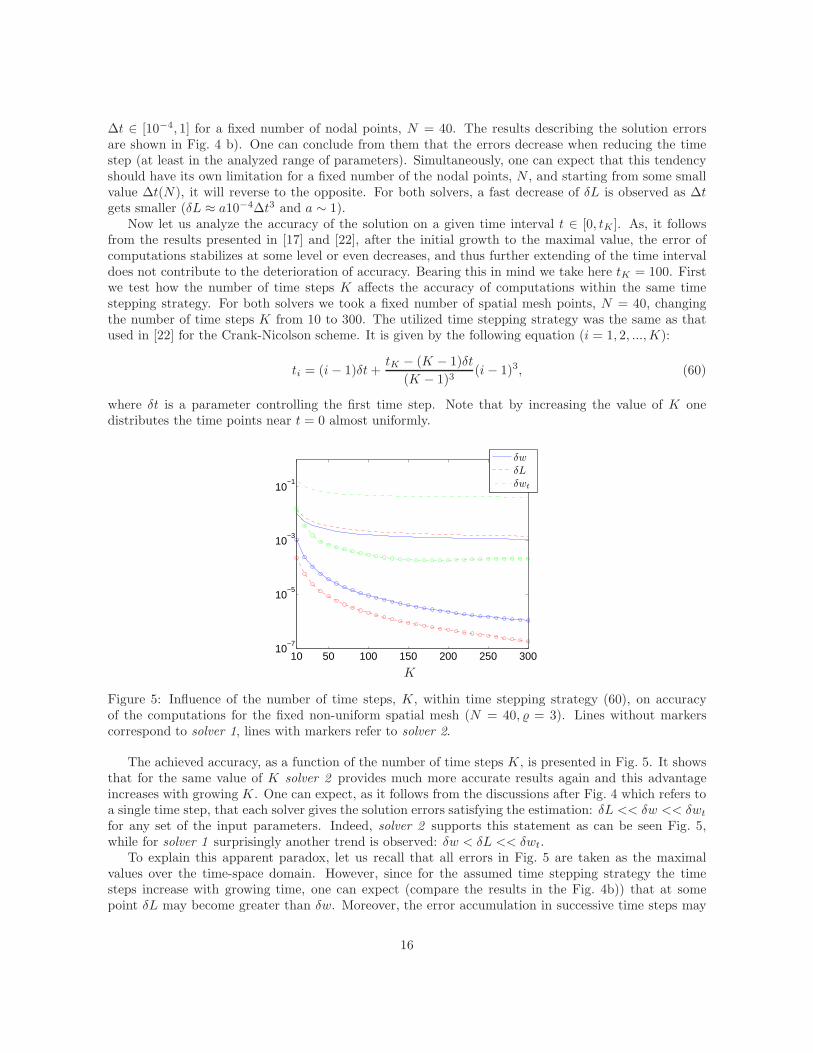
Figure 5: Influence of the number of time steps, K, within time stepping strategy (60), on accuracyof the computations for the fixed non-uniform spatial mesh (N = 40, = 3). Lines without markerscorrespond to solver 1, lines with markers refer to solver 2.

The achieved accuracy, as a function of the number of time steps K, is presented in Fig. 5. It showsthat for the same value of K solver 2 provides much more accurate results again and this advantageincreases with growing K. One can expect, as it follows from the discussions after Fig. 4 which refers toa single time step, that each solver gives the solution errors satisfying the estimation: δL << δw << δwt

for any set of the input parameters. Indeed, solver 2 supports this statement as can be seen Fig. 5,while for solver 1 surprisingly another trend is observed: δw < δL << δwt.

To explain this apparent paradox, let us recall that all errors in Fig. 5 are taken as the maximalvalues over the time-space domain. However, since for the assumed time stepping strategy the timesteps increase with growing time, one can expect (compare the results in the Fig. 4b)) that at somepoint δL may become greater than δw. Moreover, the error accumulation in successive time steps may

16

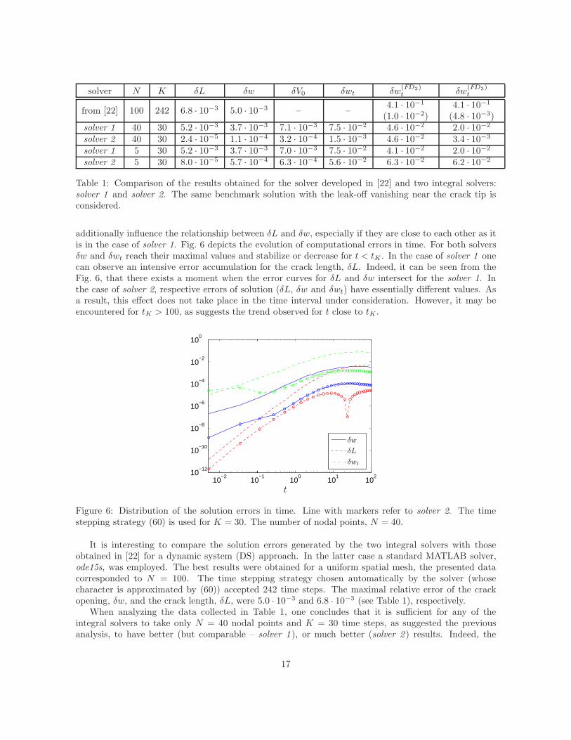
solver N K δL δw δV0 δwt δw(FD2)t δw

(FD3)t

from [22] 100 242 6.8 · 10−3 5.0 · 10−3 – –4.1 · 10−1

(1.0 · 10−2)4.1 · 10−1

(4.8 · 10−3)solver 1 40 30 5.2 · 10−3 3.7 · 10−3 7.1 · 10−3 7.5 · 10−2 4.6 · 10−2 2.0 · 10−2

solver 2 40 30 2.4 · 10−5 1.1 · 10−4 3.2 · 10−4 1.5 · 10−3 4.6 · 10−2 3.4 · 10−3

solver 1 5 30 5.2 · 10−3 3.7 · 10−3 7.0 · 10−3 7.5 · 10−2 4.1 · 10−2 2.0 · 10−2

solver 2 5 30 8.0 · 10−5 5.7 · 10−4 6.3 · 10−4 5.6 · 10−2 6.3 · 10−2 6.2 · 10−2

Table 1: Comparison of the results obtained for the solver developed in [22] and two integral solvers:solver 1 and solver 2. The same benchmark solution with the leak-off vanishing near the crack tip isconsidered.

additionally influence the relationship between δL and δw, especially if they are close to each other as itis in the case of solver 1. Fig. 6 depicts the evolution of computational errors in time. For both solversδw and δwt reach their maximal values and stabilize or decrease for t < tK . In the case of solver 1 onecan observe an intensive error accumulation for the crack length, δL. Indeed, it can be seen from theFig. 6, that there exists a moment when the error curves for δL and δw intersect for the solver 1. Inthe case of solver 2, respective errors of solution (δL, δw and δwt) have essentially different values. Asa result, this effect does not take place in the time interval under consideration. However, it may beencountered for tK > 100, as suggests the trend observed for t close to tK .

10−2

100

102

10−1

101

10−12

10−10

10−8

10−6

10−4

10−2

100

δw

δL

δwt

t

Figure 6: Distribution of the solution errors in time. Line with markers refer to solver 2. The timestepping strategy (60) is used for K = 30. The number of nodal points, N = 40.

It is interesting to compare the solution errors generated by the two integral solvers with thoseobtained in [22] for a dynamic system (DS) approach. In the latter case a standard MATLAB solver,ode15s, was employed. The best results were obtained for a uniform spatial mesh, the presented datacorresponded to N = 100. The time stepping strategy chosen automatically by the solver (whosecharacter is approximated by (60)) accepted 242 time steps. The maximal relative error of the crackopening, δw, and the crack length, δL, were 5.0 · 10−3 and 6.8 · 10−3 (see Table 1), respectively.

When analyzing the data collected in Table 1, one concludes that it is sufficient for any of theintegral solvers to take only N = 40 nodal points and K = 30 time steps, as suggested the previousanalysis, to have better (but comparable – solver 1 ), or much better (solver 2 ) results. Indeed, the

17

corresponding maximal errors for the integral solvers are: δw = 3.7 · 10−3, δL = 5.2 · 10−3 for solver1, and δw = 1.1 · 10−4, δL = 2.4 · 10−5 for solver 2. In other words, the first solver provides the sameaccuracy for the crack opening and the crack length as the DS solver using much greater numbers ofnodal points and time steps, while the second one, under the same conditions, improves the results atleast one order of magnitude. It also shows that the solver 2 yields one order of magnitude betteraccuracy of the crack propagation speed, V0, than the solver 1.

The new algorithms allow us to automatically compute the temporal derivatives in the solutionprocess. The respective errors, δwt, are: 7.5 · 10−2– solver 1 and 1.5 · 10−3 – solver 2. We decidedto compare these figures, with the ones obtained in postprocessing (here, also the DS approach wasexamined). To this end two FD schemes (2-points and 3-points) were used. This time, the correspondingerrors, δwt, were: 4.6 · 10

−2 and 2.0 · 10−2 for solver 1, 4.6 · 10−2 and 3.4 · 10−3 for solver 2 and the samevalue 4.1 · 10−1 for both schemes in the case of DS. It is worth mentioning that the values obtained forDS appeared at the first time step. Then, the errors decreased with time and stabilized to give theirminimal levels of 10−2 and 4.8 · 10−3, correspondingly.

As can be seen, the integral solvers give at least one order of magnitude better accuracy of wt thanthe DS. Moreover, while the postprocessing gives smaller (but comparable) error for the solver 1, solver2 returns more accurate values of wt than those obtained in the postprocessing, even for the 3-pointsFD. Finally, apart from the fact that δw and δL for the DS and solver 1 look comparable in values, thequality of the computation is better for the new solver as is clear from the postprocessing analysis.

Just for comparison we also present in Table 1 the results obtained for the spatial mesh composed ofonly five nodal points, N = 5. It turned out that even for such a drastic reduction of the mesh density,the solution accuracy for most of the parameters is of the same order as for N = 40. Interestingly, solver1 exhibits almost no sensitivity to this mesh reduction. In fact the distinguishable differences can beobserved only for the solver 2.

Let us now analyze the distribution of crack opening error, δw, in time and space. The respectiveresults are presented in Fig. 7 a) – solver 1, and Fig. 7 b) – solver 2. In both cases the maximal errorsare located at the crack tip while the error distribution in time follows the trend visible in Fig. 6.

0

0.5

1

0

50

1000

1

2

3

4x 10

−3

xt

δw

a)

0

0.5

1

0

50

1000

0.5

1

x 10−4

xt

δw

b)

Figure 7: The relative error of the crack opening obtained for N = 40 (nonuniform mesh, = 3) andthe time stepping strategy (60) with K = 30 . Fig. 7a) corresponds to the solver 1, while Fig. 7b) refersto the solver 2.

Fig. 8 shows the distributions of δwt obtained by the integral solvers. It confirms our previousobservation, that solver 2 always provides better results than solver 1. Moreover, the greatest error in

18

the case of solver 1 is located at the crack inlet and the lowest at the crack tip, while solver 2 givesapproximately the same values of δwt along the crack length.

0

0.5

1

0

50

1000

0.02

0.04

0.06

0.08

xt

δwt

a)

0

0.5

1

0

50

1000

0.5

1

1.5

x 10−3

xt

δwt

b)

Figure 8: The relative error of the temporal derivative of the crack opening. Solution obtained by: a)solver 1, b) solver 2 for N = 40, non-uniform mesh ( = 3) and the time step strategy (60) with K = 30.

10 50 100 150 200 250 30010

−8

10−7

10−6

10−5

10−4

δw

δL

∆wt

K

a)

10 50 100 150 200 250 30010

−6

10−4

10−2

100

δw

δL

δwt

K

b)

Figure 9: The errors of solution for two variants of γ: Fig. 9a) γ = 0, Fig. 9b) γ = 1/3. Line withmarkers correspond to solver 2.

In the last test in this subsection we analyze the relation between the regimes of crack propagationand the performances of respective solvers. As mentioned previously, the benchmark solution in form(29) can be used to imitate various dynamic modes of the crack evolution. So far we have utilized theexponent of the time dependent term of the value γ = 1/5 which refers to the constant injection fluxrate. Now, let us consider two other variants of γ: i) γ = 0 - for this choice the normalized crack openingis constant in time; ii) γ = 1/3 - this value corresponds to the steady state propagation of the fracture.For the computations the same spatial mesh as before is taken (N = 40). The number of time stepsaccepted within strategy (60), K, ranges from 10 to 300. In this way the graphs (Fig. 9a)-b)) describingthe solution errors in the function of K were prepared for both values of γ (similarly as in Fig. 5). The

19

analyzed accuracy parameters were: relative error of the crack opening, δw, relative error of crack thelength, δL, relative error of the crack opening temporal derivative, δwt, for γ = 1/3 and absolute errorof the crack opening temporal derivative, ∆wt, for γ = 0.

The results depicted in Fig. 9 show that for γ = 0 one obtains much more accurate results than forγ = 1/3 that could have been predicted (wt = 0). However, it is a surprise that for γ = 0 solver 1provides better solution accuracy than solver 2. Although the difference is moderate in case of δw andδL, the values of ∆wt vary by at least two orders of magnitude. From Fig. 9a) it follows that for thisregime of crack propagation the solution accuracy cannot be improved by simple refining the temporalmesh, and for solver 2 even a reverse relation is observed.

The situation is quite different for γ = 1/3 (Fig. 9b) ). This time again solver 2 proves its advantageover solver 1 for all the analyzed parameters. For solver 2, it is sufficient to take only 30 time steps tohave much better results than those provided by solver 1 for 300 steps. The solution accuracy can beimproved by increasing the number of time steps, however it seems that for solver 1 the saturation levelis close to K = 300. A similar trend was observed for γ = 1/5 (see Fig. 5).

A direct conclusion from this test is that for different modes of crack propagation there are differentoptimal time stepping strategies. This should properly accounted for especially in the cases when thevalues of injection flux rate or leak-off to formation change appreciably in the considered time interval.

The aforementioned analysis prove that in terms of accuracy in most of the cases solver 2 is muchbetter that solver 1 with respect to all computed components of the solution: the crack length, L,the crack opening, w, its temporal derivative, wt and the fracture propagation speed, V0. However,for some regimes of crack propagation (low values of γ) solver 1 may give comparable or even slightlybetter results than solver 2. The advantage of solver 1 is better efficiency of computations: the time ofcomputations for this solver was on average one third lower that for solver 2.

3.3.1 Example with singular leak-off regime.

In (3) we have assumed that the behaviour of the leak-off function near the crack tip can be described bya power law, giving in the worst case a square root singularity. Such a limiting behaviour corresponds tothe Carter leak-off model [5]. As a result, although the leading term of the asymptotic expansion for thecrack opening near the fracture tip remains the same, the higher terms change, disturbing the solutionsmoothness (see [15]). A comprehensive analysis of this case was done in [17] where it was also provedthat the deterioration of solution accuracy can be prevented by employing the second asymptotic termin the computational algorithm.

In this subsection we show that the algorithms developed in the paper are capable of tackling thiskind of problems without any additional modifications. To this end let us consider another benchmarksolution u(t, x) (see (63)) defined by the functions:

h(x) = (1− x)1/3(1 + s(x)), s(x) =1

5(1 − x)1/6, (61)

with the same function ψ(t) with γ = 1/5.One can easily check, that the above form of s(x) results in a singular behaviour of ql, with the

leading term of the order O(

(1− x)−1/2)

as x→ 1. The value of multiplier u0 in (63) was taken in sucha way to make the benchmark comparable with the one used previously, in a sense of an average particlevelocity. Indeed, in [22] for a fluid velocity defined as V = q/w, a parameter describing its variationalong the crack length was introduced:

γv(t) =[

maxx

(V (x, t)) −minx

(V (x, t))]

[∫ 1

0

V (x, t)dx

]−1

. (62)

This parameter reflects indirectly the balance between the flux injection rate and leak-off to formation.It was also shown there that it has a decisive influence on the accuracy of computations (the greater

20

value of γv, the greater error of the computations). For the benchmarks with comparable values of γv,one can expect similar accuracy of the computations. This trend was also confirmed in [17]. In our case,the deterioration of the solution smoothness near the crack tip is an additional factor which contributesto the increase of the computational error.

Note that because of the chosen structure of (63), the value of γv is constant in time for all benchmarksconsidered in this paper. For the benchmark (43) γv yields 0.408, while (61) one leads to γv = 0.411.

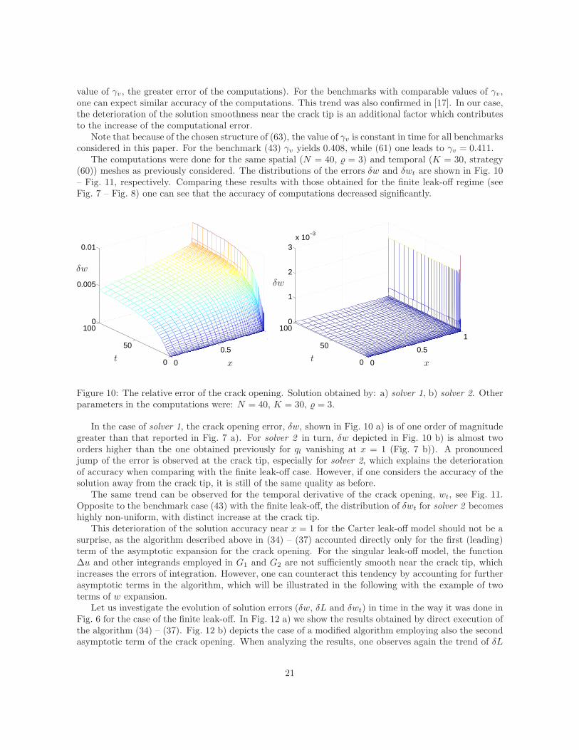
The computations were done for the same spatial (N = 40, = 3) and temporal (K = 30, strategy(60)) meshes as previously considered. The distributions of the errors δw and δwt are shown in Fig. 10– Fig. 11, respectively. Comparing these results with those obtained for the finite leak-off regime (seeFig. 7 – Fig. 8) one can see that the accuracy of computations decreased significantly.

0

0.5

1

0

50

1000

0.005

0.01

xt

δw

0

0.5

1

0

50

1000

1

2

3x 10

−3

xt

δw

Figure 10: The relative error of the crack opening. Solution obtained by: a) solver 1, b) solver 2. Otherparameters in the computations were: N = 40, K = 30, = 3.

In the case of solver 1, the crack opening error, δw, shown in Fig. 10 a) is of one order of magnitudegreater than that reported in Fig. 7 a). For solver 2 in turn, δw depicted in Fig. 10 b) is almost twoorders higher than the one obtained previously for ql vanishing at x = 1 (Fig. 7 b)). A pronouncedjump of the error is observed at the crack tip, especially for solver 2, which explains the deteriorationof accuracy when comparing with the finite leak-off case. However, if one considers the accuracy of thesolution away from the crack tip, it is still of the same quality as before.

The same trend can be observed for the temporal derivative of the crack opening, wt, see Fig. 11.Opposite to the benchmark case (43) with the finite leak-off, the distribution of δwt for solver 2 becomeshighly non-uniform, with distinct increase at the crack tip.

This deterioration of the solution accuracy near x = 1 for the Carter leak-off model should not be asurprise, as the algorithm described above in (34) – (37) accounted directly only for the first (leading)term of the asymptotic expansion for the crack opening. For the singular leak-off model, the function∆u and other integrands employed in G1 and G2 are not sufficiently smooth near the crack tip, whichincreases the errors of integration. However, one can counteract this tendency by accounting for furtherasymptotic terms in the algorithm, which will be illustrated in the following with the example of twoterms of w expansion.

Let us investigate the evolution of solution errors (δw, δL and δwt) in time in the way it was done inFig. 6 for the case of the finite leak-off. In Fig. 12 a) we show the results obtained by direct execution ofthe algorithm (34) – (37). Fig. 12 b) depicts the case of a modified algorithm employing also the secondasymptotic term of the crack opening. When analyzing the results, one observes again the trend of δL

21

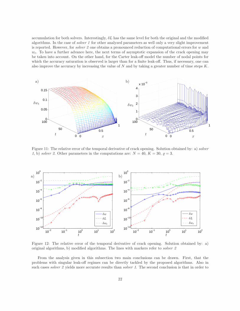
accumulation for both solvers. Interestingly, δL has the same level for both the original and the modifiedalgorithms. In the case of solver 1 for other analyzed parameters as well only a very slight improvementis reported. However, for solver 2 one obtains a pronounced reduction of computational errors for w andwt. To have a further advance here, the next terms of asymptotic expansion of the crack opening maybe taken into account. On the other hand, for the Carter leak-off model the number of nodal points forwhich the accuracy saturation is observed is larger than for a finite leak-off. Thus, if necessary, one canalso improve the accuracy by increasing the value of N and by taking a greater number of time steps K.

0

0.5

1

0

50

1000

0.05

0.1

0.15

xt

δwt

a)

0

0.5

150

100

0

0

1

2

3

4x 10

−3

xt

δwt

b)

Figure 11: The relative error of the temporal derivative of crack opening. Solution obtained by: a) solver1, b) solver 2. Other parameters in the computations are: N = 40, K = 30, = 3.

10−2

100

102

10−1

101

10−12

10−10

10−8

10−6

10−4

10−2

100

δw

δL

δwt

t

a)

10−2

100

102

10−1

101

10−12

10−10

10−8

10−6

10−4

10−2

100

δw

δL

δwt

t

b)

Figure 12: The relative error of the temporal derivative of crack opening. Solution obtained by: a)original algorithms, b) modified algorithms. The lines with markers refer to solver 2

From the analysis given in this subsection two main conclusions can be drawn. First, that theproblems with singular leak-off regimes can be directly tackled by the proposed algorithms. Also insuch cases solver 2 yields more accurate results than solver 1. The second conclusion is that in order to

22

have the solution accuracy comparable to that achieved for non-singular leak-off, one has to use a largernumber of nodal points and/or employ further terms of asymptotic expansion for w in the algorithm.

4 Conclusions

We would like to itemize the following conclusions as a resume of this paper:

• Presented approach can be efficiently used for tackling the PKN model of hydrofracturing and maybe adopted for multifracture systems.

• Both new solvers provide better computational accuracy than the conventional algorithms from[22]. Moreover, comparable accuracies can be achieved here at much lower computational cost, asthe new solvers enable us to drastically reduce the densities of spatial and temporal meshes.

• New solvers are appropriate for directly tackling the problems with different fluid flow regimes,including various injection flux rates and singular leak-off.

• In order to increase the efficiency and accuracy of computations, it is advisable to employ at leasttwo asymptotic terms of the crack opening, w.

• The developed algorithms do not require any regularization techniques. The boundary conditionsare imposed directly into the numerical scheme. The speed equation plays a crucial role in theanalysis.

Acknowledgements

This work has been done in the framework of the EU FP7 PEOPLE project under contract numberPIAP-GA-2009-251475-HYDROFRAC. The authors are grateful to the Institute of Mathematics andPhysics of Aberystwyth University and EUROTECH Sp. z o. o. for the facilities and hospitality.

References

[1] Adachi J, Detournay E (2002) Self-similar solution of a plane-strain fracture driven by a power-lawfluid. Int J Numer Anal Methods Geomech 26: 579-604

[2] Adachi J, Detournay E (2008) Plane strain propagation of a hydraulic fracture in a permeable rock.Eng Fract Mech 75(16): 4666-4694

[3] Adachi J, Peirce A (2007) Asymptotic analysis of an elasticity equation for a finger-like hydraulicfracture. J Elast 90(1): 43-69

[4] Adachi J, Siebrits E, Peirce A, Desroches J (2007) Computer simulation of hydraulic fractures. IntJ Rock Mech Min Sci 44: 739-757

[5] Carter E (1957) Optimum fluid characteristics for fracture extension. In: Howard, G., Fast, C.(eds.) Drilling and Production Practices, 261-270. American Petroleum Institute

[6] Crittendon BC (1959) The mechanics of design and interpertation of hydraulic fracture treatments.J Pet Tech 21: 21-29

[7] Detournay E (2004) Propagation regimes of fluid-driven fractures in impermeable rocks. Int J Geom4: 1-11

23

[8] Dobroskok AA, Linkov AM (2011) Modeling of fluid flow, stress state and seismicity induced inrock by instant pressure drop in a hydrofracture. J Min Sci 47(1): 10-19

[9] Economides M, Nolte K (eds.) (2000) Reservoir Stimulation. 3rd edn. Wiley, Chichester, UK

[10] Garagash DI, Detournay E (2000) The tip region of a fluid-driven fracture in an elastic medium. JAppl Mech 67: 183-192

[11] Geertsma J, de Klerk F (1969) A rapid method of predicting width and extent of hydraulicallyinduced fractures. J Pet Tech 21: 1571-1581 [SPE 2458]

[12] Hubbert MK, Willis DG (1957) Mechanics of hydraulic fracturing. J. Pet. Tech. 9(6): 153-68

[13] Kemp LF (1989) Study of Nordgren’s equation of hydraulic fracturing. SPE Production Eng 5:311-314

[14] Khristianovic SA, Zheltov YP (1955) Formation of vertical fractures by means of highly viscousliquid. In: Proceedings of the fourth world petroleum congress, Rome, 1955, 579-586

[15] Kovalyshen Y, Detournay E (2009) A reexamination of the classical PKN model of hydraulic frac-ture. Transp Porous Med 81: 317-339

[16] Kovalyshen Y (2010) Fluid-driven fracture in poroelastic medium. PhD Thesis, The University ofMinnesota

[17] Kusmierczyk P, Mishuris G, Wrobel M (2012) Remarks on numerical simulation of the PKN modelof hydrofracturing in proper variables. Various leak-off regimes. arXiv:1211.6474.

[18] Lecampion B, Detournay E (2007) An implicit algorithm for the propagation of a hydraulic fracturewith a fluid lag. Comput Method Appl M 196(49-52): 4863 – 4880

[19] Linkov AM (2011) Speed equation and its application for solving ill-posed problems of hydraulicfracturing. ISSM 1028-3358, Doklady Physics, 56(8): 436-438. Pleiades Publishing, Ltd.

[20] Linkov AM (2011) Use of a speed equation for numerical simulation of hydraulic fractures.arXiv:1108.6146

[21] Linkov AM (2011) On efficient simulation of hydraulic fracturing in terms of particle velocity. Int JEngng Sci 52: 77-88

[22] Mishuris G, Wrobel M, Linkov A (2012) On modeling hydraulic fracture in proper variables: stiff-ness, accuracy, sensitivity. Int J Engng Sci 61: 10-23

[23] Mitchell SL, Kuske R, Peirce A (2007) An asymptotic framework for finite hydraulic fracturesincluding leakoff. SIAM J Appl Math 67(2): 364–386

[24] Mitchell SL, Kuske R, Peirce AP (2007) An asymptotic framework for the analysis of hydraulicfractures: the impermeable case. ASME J Appl Mech 74(2): 365–372

[25] Moos D (2012) The importance of stress and fractures in hydrofracturing and stimulation perfor-mance: a geomechanics overview. Search and Discovery Article 80255 (2012)

[26] Nordgren, RP (1972) Propagation of a Vertical Hydraulic Fracture. J Pet Tech 253: 306-314

[27] Olson JE (2008) Multi-fracture propagation modeling: Applications to hydraulic fracturing in shalesand tight gas sands. The 42nd U.S. Rock Mechanics Symposium (USRMS), June 29 - July 2, 2008,San Francisco, CA

24

[28] Peirce A, Detournay E (2008). An implicit level set method for modeling hydraulically drivenfractures. Comput Methods Appl Mech Engrg 197: 2858–2885

[29] Peirce A, Detournay E (2009), An eulerian moving front algorithm with weak-form tip asymptoticsfor modeling hydraulically driven fractures. Num Meth Eng 25(2): 185-200

[30] Perkins TK, Kern LR (1961) Widths of hydraulic fractures. J Pet Tech 13(9): 37-49 [SPE 89]

[31] Rubin AM (1995) Propagation of magma filled cracks. Ann Rev Earth Planet Sci 23: 287-336

[32] Sneddon IN, Elliot HA (1946) The opening of a Griffith crack under internal pressure. Q Appl Math4: 262-267

[33] Stoer J, Bulirsh R (2002) Introduction to Numerical Analysis. Third Edition. Springer-Verlag.

[34] Tsai VC, Rice JR (2010) A model for turbulent hydraulic fracture and application to crack propa-gation at glacier beds. J Geophys Res 115: 1-18

[35] Zhang X, Jeffrey R, Llanos EM (2004) A study of shear hydraulic fracture propagation. Gulf Rocks2004, the 6th North America Rock Mechanics Symposium (NARMS), June 5 - 9, 2004 , Houston,Texas

Appendix A: Numerical benchmarks

Let us define a set of benchmark solutions useful for testing different numerical solvers. Consider a classof positive functions C+(0, 1) described in the following manner:

C+(0, 1) = {h ∈ C2(0, 1) ∩ C[0, 1],

limx→1−

(1− x)−1/3h(x) = 1, h(x) > 0, x ∈ [0, 1)}.

By taking an arbitrary h ∈ C+(0, 1), one can build a benchmark solution for the normalized formulationof the problem as:

u(x) = u0ψj(t)h(x). (63)

where functions ψj(t) and h(x) are specified below. On substitution of (63) into (26) one finds:

ql(t, x) = (64)

γu0[ 1

β

(

xh3(x)h′(x) + 3(

h3(x)h′(x))′)

− h(x)]

ψαj (t),

w0(t) = u0ψj(t),

where two sets of the benchmark solutions can be considered. For the first one we choose ψ1(t) = eγt

and β = 2/3, α = 1, while for the second, ψ2(t) = (a + t)γ and β = 2γ/(3γ + 1), α = (3γ − 1)/γ.Corresponding crack lengths are defined in (25) and (30), respectively. Finally, the injection flux rate iscomputed from the boundary condition (16)1:

q0(t) = −u40ψ

4j (t)

L(t)h3(0)h′(0), (65)

while the initial condition reads W (x) = u0ψj(0)h(x).

25

Note that when taking the function h(x) from the class C+(0, 1) in the following representation:

h(x) = (1− x)1/3(1 + s(x)),

s ∈ C2[0, 1], s(x) > −1, x ∈ [0, 1)

ql automatically satisfies the condition ql(t, x) = O(

(1− x)1/3)

, x→ 1.The presented benchmarks allow one to test numerical schemes in various fracture propagation

regimes (accelerating/decelerating cracks) by choosing proper values of the parameter γ (see [22]).Additionally, if one reduces the requirements for the smoothness of s(x) near x = 1, assuming thath ∈ C2[0, 1)

⋂

Hα(0, 1) the benchmark can serve to model singular leak-off regimes (compare with (61)).Note that the zero leak-off case cannot be described by the aforementioned group of benchmarks.

However, an analytical benchmark for this regime, represented in terms of a rapidly converging series,has been developed in [21].

26