ECEN 615 Methods of Electric Power Systems Analysis Lecture 16...
43
Lecture 16: Sensitivity Analysis ECEN 615 Methods of Electric Power Systems Analysis Prof. Tom Overbye Dept. of Electrical and Computer Engineering Texas A&M University [email protected]
Transcript of ECEN 615 Methods of Electric Power Systems Analysis Lecture 16...

Lecture 16: Sensitivity Analysis
ECEN 615Methods of Electric Power Systems Analysis
Prof. Tom Overbye
Dept. of Electrical and Computer Engineering
Texas A&M University

Announcements
• Exam average was 85.7, with a high of 100
• Read Chapter 7 (the term reliability is now used instead
of security)
• Homework 4 is assigned today, due on Thursday Nov 1
2

Linearized Sensitivity Analysis
• By using the approximations from the fast
decoupled power flow we can get sensitivity values
that are independent of the current state. That is,
by using the B’ and B’’ matrices
• For line flow we can approximate
3
2
( ) ( ) ( ), ,
By using the FDPF appxomations
( )( ) ( ) , ,
i i j i j i j i j
i ji j
h s g V V V cos b V V sin i j
h s b i jX

Linearized Sensitivity Analysis
• Also, for each line
and so,
0
4
0V
h
a
θ
hb
1 1
h
a a A Bθh
x 0h
V
L
TL
b b
0

Sensitivity Analysis: Recall the Matrix Notation
• The series admittance of line is g +jb and we
define
• We define the LN incidence matrix
5
1 2B , , ,
Ldiag b b b
1
2
a
aA
aL
T
T
T
where the component j of ai isnonzero whenever line i is
coincident with node j. Hence
A is quite sparse, with at most
two nonzeros per row

Linearized Active Power Flow Model
• Under these assumptions the change in the real power
line flows are given as
• The constant matrix
is called the injection shift factor matrix (ISF)
1
1B 0 I
f B A 0 p B A B p Ψ p0 B 0
1Ψ BA B
6

Injection Shift Factors (ISFs)
• The element in row and column n of is called
the injection shift factor (ISF) of line with respect to
the injection at node n
– Absorbed at the slack bus, so it is slack bus dependent
• Terms generation shift factor (GSF) and load shift
factor (LSF) are also used (such as by NERC)
– Same concept, just a variation in the sign whether it is a
generator or a load
– Sometimes the associated element is not a single line, but
rather a combination of lines (an interface)
• Terms used in North America are defined in the NERC
glossary (http://www.nerc.com/files/glossary_of_terms.pdf)
n
7

line
np
n nf
i j
slackbusp
ISF Interpretation
is the fraction of the additional 1 MW injection atnode n that goes though line
+ 1
n
slack
node
1
8

ISF Properties
• By definition, depends on the location of the
slack bus
• By definition, for since the
injection and withdrawal buses are identical in this case and, consequently, no flow arises on any line
• The magnitude of is at most 1 since
n
1 1n
slackbus0 L
n
Note, this is strictly true only for the linear (lossless)
case. In the nonlinear case, it is possible that a
transaction decreases losses. Hence a 1 MW injection
could change a line flow by more than 1 MW.9

Five Bus Example Reference
Line 1
Line 2
Line 3
Line 6
Line 5
Line 4slack
1.050 pu
42 MW
67 MW
100 MW
118 MW
1.040 pu
1.042 pu
A
MVA
A
MVA
A
MVA
1.042 pu
A
MVA
1.044 pu
33 MW
MW200
258 MW
MW118
260 MW
100 MW
MW100
A
MVA
One Two
Three
Four
Five
10
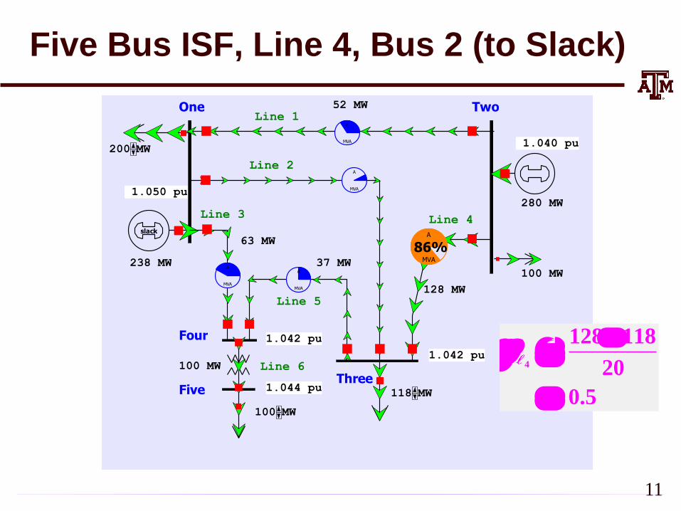
Five Bus ISF, Line 4, Bus 2 (to Slack)
Line 1
Line 2
Line 3
Line 6
Line 5
Line 4slack
1.050 pu
52 MW
63 MW
100 MW
128 MW
1.040 pu
1.042 pu
A
MVA
A
MVA
1.042 pu
A
MVA
1.044 pu
37 MW
MW200
238 MW
MW118
280 MW
100 MW
MW100
A
MVA
One Two
Three
Four
Five
86%A
MVA
4
2 128 118
20
0.5
11

Five Bus Example
-1 0 0 0
0 -1 0 0
0 0 -1 0A
1 -1 0 0
0 1 -1 0
0 0 1 -1
=
The row of A correspond to
the lines and transformers,
the columns correspond to
the non-slack buses (buses 2
to 5); for each line there
is a 1 at one end, a -1 at the
other end (hence an
assumed sign convention!).
Here we put a 1 for the
lower numbered bus, so
positive flow is assumed
from the lower numbered
bus to the higher number
B 6.25, 12.5, 12.5, 12.5, 12.5, 10= diag
12

Five Bus Example
18.75 12.5
12.5 37.5 12.5B A B A
12.5 35 10
10 10
T
0 0
0= =
0
0 0
1
-0.4545 -0.1818 -0.0909 -0.0909
-0.3636 -0.5455 -0.2727 -0.2727
-0.1818 -0.2727 -0.6364 -0.6364
0.5455 -0.1818 -0.0909 -0.0909
0.1818 0.2727 -0.3636 -0.3636
-1.0000
B A B
0 0 0
13With bus 1 as the slack, the buses (columns) go for 2 to 5

Five Bus Example Comments
• At first glance the numerically determined value of
(128-118)/20=0.5 does not match closely with the
analytic value of 0.5455; however, in doing the
subtraction we are losing numeric accuracy
– Adding more digits helps (128.40 – 117.55)/20 = 0.5425
• The previous matrix derivation isn’t intended for actual computation; is a full matrix so we would
seldom compute all of its values
• Sparse vector methods can be used if we are only
interested in the ISFs for certain lines and certain
buses
14

Distribution Factors
• Various additional distribution factors may be
defined – power transfer distribution factor (PTDF)
– line outage distribution factor (LODF)
– line addition distribution factor (LADF)
– outage transfer distribution factor (OTDF)
• These factors may be derived from the ISFs making
judicious use of the superposition principle
15

Definition: Basic Transaction
• A basic transaction involves the transfer of a
specified amount of power t from an injection node
m to a withdrawal node n
t
n
t
m
16

Definition: Basic Transaction
• We use the notation
to denote a basic transaction
injection
node withdrawal
node quantity
, ,w m n t
17

Definition: PTDF
• NERC defines a PTDF as
– “In the pre-contingency configuration of a system under
study, a measure of the responsiveness or change in
electrical loadings on transmission system Facilities due
to a change in electric power transfer from one area to
another, expressed in percent (up to 100%) of the change
in power transfer”
– Transaction dependent
• We’ll use the notation to indicate the PTDF
on line with respect to basic transaction w
• In the lossless formulation presented here (and
commonly used) it is slack bus independent
( )w
18

PTDFs
line
nf
i j
t
m
t
f
t+t+
( )w f
t
Note, the PTDF is
independent of the
amount t; which is often
expressed as a percent19

PTDF Evaluation in Two Parts
line
( )w
i j
nm
1
=
m
i j
0+
m
1
1
1
i j
0
n
1
n
1 20

line
nf
i j
t
m
t
0
PTDF Evaluation
+ 1 + 1
m n
1 1
( )w m n
21

Calculating PTDFs in PowerWorld
• PowerWorld provides a number of options for
calculating and visualizing PTDFs
– Select Tools, Sensitivities, Power Transfer Distribution
Factors (PTDFs)
Results are
shown for the
five bus case
for the Bus 2
to Bus 3
transaction
22

Five Bus PTDF Visualization
Line 1
Line 2
Line 3
Line 6
Line 5
Line 4slack
1.050 pu
52 MW
63 MW
100 MW
128 MW
1.040 pu
1.042 pu
9%PTDF
27%PTDF
73%PTDF
1.042 pu
9%PTDF
1.044 pu
37 MW
MW200
238 MW
MW118
280 MW
100 MW
MW100
18%PTDF
One Two
Three
Four
Five
PowerWorld Case: B5_DistFact_PTDF 23

Nine Bus PTDF Example
slack
43%PTDF
57%PTDF
13%PTDF
30%PTDF
35%PTDF
20%PTDF
10%PTDF
2%PTDF
34%PTDF
34%PTDF
32%PTDF
A
G
B
C
D
E
I
F
H
34%PTDF
MW 400.0 MW 400.0 MW 300.0
MW 250.0
MW 250.0
MW 200.0
MW 250.0
MW 150.0
50.0 MW
PowerWorld Case: B9_PTDF
Display shows
the PTDFs
for a basic
transaction
from Bus A
to Bus I. Note
that 100% of
the transaction
leaves Bus A
and 100%
arrives at
Bus I24

Eastern Interconnect Example: Wisconsin Utility to TVA PTDFs
In this
example
multiple
generators
contribute
for both
the seller
and the
buyer
Contours show lines that would carry at least 2% of a
power transfer from Wisconsin to TVA 25

Line Outage Distribution Factors (LODFs)
• Power system operation is practically always limited
by contingencies, with line outages comprising a large
number of the contingencies
• Desire is to determine the impact of a line outage
(either a transmission line or a transformer) on other
system real power flows without having to explicitly
solve the power flow for the contingency
• These values are provided by the LODFs
• The LODF is the portion of the pre-outage real power line flow on line k that is redistributed to line as a result of the outage of line k
26
kd

line
f
i j
LODFs
f
kline
kf
i j
line
f
i j
outaged
klinei j
,k
k
k
fd d
f
base caseoutage case
Best reference is Chapter 7 of the course book27

LODF Evaluation
We simulate the impact of the outage of line k by
adding the basic transaction , ,k k
w i j t
and selecting tk in such
a way that the flows on
the dashed lines become
exactly zeroline
f f
i j
kline
i j
kt k
t
k kf f
In general this tk is not
equal to the original line
flow
28

LODF Evaluation
• We select tk to be such that
where ƒ k is the active power flow change on the line
k due to the transaction wk
• The line k flow from wk depends on its PTDF
it follows that
kk kf f t 0
( )kw
k kkf t
( )1 1k
k k
k w i j
k k k
f ft
29

LODF Evaluation
• For the rest of the network, the impacts of the
outage of line k are the same as the impacts of the
additional basic transaction wk
• Therefore, by definition the LODF is
( )
( )
( )1
k
k
k
w
w
k w
k
kf t f
( )
( )1
k
k
w
k
w
k k
fd
f
30

Five Bus Example
• Assume we wish to calculate the values for the outage
of line 4 (between buses 2 and 3); this is line k
Line 1
Line 2
Line 3
Line 6
Line 5
Line 4slack
1.050 pu
52 MW
63 MW
100 MW
128 MW
1.040 pu
1.042 pu
A
MVA
A
MVA
1.042 pu
A
MVA
1.044 pu
37 MW
MW200
238 MW
MW118
280 MW
100 MW
MW100
A
MVA
One Two
Three
Four
Five
86%A
MVA
Say we wish
to know
the change
in flow
on the line
3 (Buses 3
to 4).
PTDFs for
a transaction
from 2 to 3
are 0.7273
on line 4
and 0.0909
on line 3 31

Five Bus Example
• Hence we get
4
4
( )
3 34
3 ( )
4 4
3 4
0.09090.333
1 1 0.7273
0.333 0.333 128 42.66MW
w
w
fd
f
f f
( )
128469.4
1 1 0.7273k
k
k w
k
ft
32

Five Bus Example Compensated
Line 1
Line 2
Line 3
Line 6
Line 5
Line 4slack
1.050 pu
184 MW
108 MW
100 MW
465 MW
1.040 pu
1.016 pu
A
MVA
1.027 pu
A
MVA
1.029 pu
8 MW
MW200
238 MW
MW587
749 MW
100 MW
MW100
A
MVA
One Two
Three
Four
Five
124%A
MVA
312%A
MVA
Here is the
system with the
compensation
added to bus
2 and removed
at bus 3; we
are canceling
the impact of
the line 4 flow
for the reset
of the network.
33

Five Bus Example
• Below we see the network with the line actually
outaged
Line 1
Line 2
Line 3
Line 6
Line 5
Line 4slack
1.050 pu
180 MW
106 MW
100 MW
0 MW
1.040 pu
1.044 pu
A
MVA
1.042 pu
A
MVA
1.044 pu
6 MW
MW200
238 MW
MW118
280 MW
100 MW
MW100
A
MVA
One Two
Three
Four
Five
121%A
MVA
The line 3
flow changed
from 63 MW
to 106 MW,
an increase
of 43 MW,
matching the
LODF
value
34

Developing a Critical Eye
• In looking at the below formula you need to be
thinking about what conditions will cause the formula
to fail
Here the obvious situation is when the denominator is
zero
• That corresponds to a situation in which the
contingency causes system islanding
– An example is line 6 (between buses 4 and 5)
– Impact modeled by injections at the buses within each viable
island
( )
( )
( )1
k
k
k
w
w
k w
k
kf t f
35

Calculating LODFs in PowerWorld
• Select Tools, Sensitivities, Line Outage Distribution
Factors
– Select the Line using dialogs on right, and click Calculate
LODFS; below example shows values for line 4
36

Blackout Case LODFs
• One of the issues associated with the 8/14/03 blackout
was the LODF associated with the loss of the Hanna-
Juniper 345 kV line (21350-22163) that was being
used in a flow gate calculation was not correct because
the Chamberlin-Harding 345 kV line outage was
missed
– With the Chamberlin-Harding line assumed in-service the
value was 0.362
– With this line assumed out-of-service (which indeed it was)
the value increased to 0.464
37

2000 Bus LODF Example
LODF is for line
between 3048 and
5120; values will
be proportional to
the PTDF values
38

2000 Bus LODF Example
0%PTDF
0%
PTDF
0%
PTDF
0%
PTDF
0%
PTDF
0%
PTDF
0%
PTDF
0%
PTDF
0%
PTDF
0%
PTDF 0%
PTDF
0%
PTDF
0%
PTDF 0%
PTDF
0%
PTDF
0%
PTDF
0%
PTDF
1%PTDF
0%
PTDF
0%
PTDF
0%
PTDF
0%
PTDF 0%
PTDF
0%
PTDF
0%
PTDF
0%
PTDF
0%
PTDF
0%PTDF
0%PTDF
0%PTDF
0%
PTDF
0%
PTDF
0%
PTDF
0%
PTDF
0%
PTDF
0%PTDF
0%PTDF
0%
PTDF
0%
PTDF
0%
PTDF
0%
PTDF
0%
PTDF
0%
PTDF
0%
PTDF
0%
PTDF
0%
PTDF
0%
PTDF
0%
PTDF
0%
PTDF
0%
PTDF
0%
PTDF
0%
PTDF
0%
PTDF
0%
PTDF
0%
PTDF
0%
PTDF
0%
PTDF
0%
PTDF
0%
PTDF 0%
PTDF
0%
PTDF
0%
PTDF
0%PTDF
0%
PTDF
0%
PTDF
0%
PTDF
0%
PTDF
0%
PTDF
0%
PTDF
0%
PTDF
0%
PTDF
0%
PTDF
1%PTDF
0%PTDF
0%
PTDF
0%
PTDF
0%
PTDF
0%
PTDF 0%PTDF
0%PTDF
0%
PTDF
0%
PTDF
0%
PTDF
0%
PTDF
0%
PTDF
0%
PTDF
0%
PTDF
0%
PTDF
0%
PTDF
0%
PTDF
0%
PTDF
0%
PTDF
0%PTDF
0%
PTDF
0%
PTDF
0%
PTDF
0%
PTDF
0%
PTDF
0%
PTDF
0%
PTDF
0%
PTDF
0%
PTDF
0%
PTDF
1%
PTDF
0%PTDF
0%
PTDF
0%
PTDF
0%
PTDF
0%
PTDF
0%
PTDF
0%
PTDF
0%
PTDF
0%
PTDF
0%PTDF
0%
PTDF
0%
PTDF
1%PTDF
1%PTDF
0%
PTDF
1%PTDF
1%PTDF 19%
PTDF 19%PTDF
49%PTDF
7%PTDF
0%PTDF
1%PTDF
1%PTDF
0%
PTDF
0%
PTDF
0%
PTDF
0%
PTDF
0%
PTDF
0%
PTDF
0%
PTDF
1%PTDF
0%
PTDF
0%PTDF 0%
PTDF
2%
PTDF
1%PTDF
0%
PTDF
0%
PTDF
0%
PTDF
0%
PTDF
0%
PTDF
0%
PTDF
0%
PTDF
0%
PTDF
0%
PTDF
0%
PTDF
0%
PTDF
0%
PTDF
1%
PTDF
0%
PTDF
0%
PTDF
0%
PTDF
0%
PTDF
2%PTDF
0%PTDF
2%PTDF
0%PTDF
3%PTDF
3%PTDF 3%PTDF
4%PTDF
0%
PTDF
1%PTDF
2%PTDF
1%PTDF
1%
PTDF
0%PTDF
1%PTDF
31%PTDF
6%PTDF
0%PTDF
1%
PTDF
3%PTDF
2%PTDF
0%PTDF
0%PTDF
1%PTDF
0%PTDF
0%
PTDF
0%
PTDF
0%
PTDF
2%PTDF
0%
PTDF
0%
PTDF
0%PTDF
1%PTDF
0%PTDF
0%
PTDF
2%
PTDF
0%
PTDF
0%
PTDF
0%
PTDF
0%
PTDF
0%PTDF
0%
PTDF
0%
PTDF
0%
PTDF
0%PTDF 1%
PTDF
1%PTDF
0%
PTDF
1%
PTDF
0%
PTDF
0%
PTDF
0%
PTDF
0%
PTDF
1%
PTDF
1%
PTDF
0%
PTDF
17%PTDF
0%
PTDF
0%
PTDF
0%
PTDF
0%
PTDF
0%
PTDF
1%
PTDF
1%
PTDF
4%PTDF
3%PTDF
0%
PTDF
0%
PTDF
0%
PTDF
0%
PTDF
0%
PTDF
6%PTDF
0%
PTDF
0%
PTDF
0%
PTDF
0%
PTDF
0%
PTDF
0%
PTDF
0%
PTDF
0%
PTDF 1%
PTDF
0%
PTDF
2%PTDF
2%PTDF
0%
PTDF
5%PTDF
3%PTDF
1%PTDF
0%PTDF
1%
PTDF
0%
PTDF
0%
PTDF
0%
PTDF
2%PTDF
0%
PTDF
1%PTDF
0%
PTDF
0%
PTDF
0%
PTDF
0%
PTDF
0%
PTDF
6%PTDF
11%PTDF
5%PTDF
0%
PTDF
0%
PTDF
0%
PTDF
0%
PTDF
0%
PTDF
0%
PTDF
0%
PTDF
4%PTDF
0%
PTDF
0%PTDF
5%PTDF
2%PTDF
0%
PTDF
2%
PTDF
0%PTDF
1%PTDF
2%PTDF
3%PTDF
1%PTDF
0%
PTDF
1%
PTDF
4%PTDF
0%
PTDF
0%
PTDF
1%PTDF
0%
PTDF
0%
PTDF
0%
PTDF
0%
PTDF
0%
PTDF
0%
PTDF
0%
PTDF
0%
PTDF
0%
PTDF
0%
PTDF
0%
PTDF
0%
PTDF
0%
PTDF
0%
PTDF
0%
PTDF
0%
PTDF
0%
PTDF
0%
PTDF
0%
PTDF
0%
PTDF
0%
PTDF
1%PTDF
0%PTDF
0%
PTDF
0%
PTDF
0%
PTDF
0%
PTDF
0%
PTDF
0%PTDF
1%PTDF
0%PTDF
0%
PTDF
0%
PTDF
1%PTDF
0%
PTDF
0%
PTDF
1%PTDF
0%
PTDF
0%
PTDF
0%
PTDF
0%
PTDF
0%
PTDF
0%
PTDF
0%
PTDF
0%
PTDF
0%
PTDF
0%PTDF
L ENORAH
GOL DSBORO
SWEETWATER 3
WINTERS
SWEETWATER 1
ROWENA
TRENT 2
SANTA ANNA
STANTON
GOODFEL L OW AFB
EDEN
ABIL ENE 5
MIDL AND 5
BIG L AKE
SAN ANGEL O 3
ROSCOE 3
SWEETWATER 2
L AMPASAS
ODONNEL L
BANGS
WACO 3
GROESBECK
MABANK 2
COMO
WACO 4
L ORENA
STREETMAN
EVANT
TERREL L 1
GATESVIL L E 4
CL EBURNE 2
DECATUR
THORNTON
EARL Y
TROY
GRAPEL AND
CANTON
FORT HOOD
CUMBY
MAL AKOFF
COMANCHE
TEAGUE
HICO
PAL O PINTO 2
MIL FORD
CL IFTON 1
MOUNT VERNON
FROST
YANTIS
BARDWEL L
AL BANY 2
KERENS
L IPAN
MONTAGUE
DODD CITYSEYMOUR
SPUR
ARCHER 1
NOCONA
ARCHER 2
L AMESA
ASPERMONT
MCCAMEY 2
MUENSTER 1
COL L INSVIL L E
JAYTON
BIG SPRING 3
ODESSA 3
MIDL AND 1
ARCHER CITY
TRENTON
TEL EPHONE
BIG SPRING 6
MUENSTER 2
BIG SPRING 2
DENISON 1
ROCHESTER
SHERMAN 2
WHITEWRIGHT
RAL L S 2
ECTOR
SUNSET
SHERMAN 3
L INDSAY
SADL ER
FORESTBURG
MATADOR BONHAM
KNOX CITYL EONARD
HONEY GROVE
ROXTON
BOWIE
SUMNER
GAINESVIL L E
DENISON 2
PARIS 3
BEL L S
WHITESBORO
PATTONVIL L E
HENRIETTA
CROSBYTON
O DONNEL L 2
HAWL EY
DYESS AFB
BIG SPRING 1
MERKEL 2
SWEETWATER 5
ABIL ENE 3
MIL ES
NOL AN
TRENT 1
OVAL O
ABIL ENE 6
L ORAINE 1
SYNDER
ROTAN
BIG SPRING 4
FORSAN
ROSCOE 1
MIDL AND 2
FL UVANNA 1
KEMPNER
BIG SPRINGS
SAN ANGEL O 2
STERL ING CITY 2
COAHOMA
MIDL AND 3
BRADY
BIG SPRING 5
ABIL ENE 4
COL ORADO CITY
STAMFORD
BL ACKWEL L
L UEDERS
HAML IN
MERKEL 3
HASKEL L
SAINT JO
COL EMAN
ODESSA 2
RICHL AND SPRINGS
BAL L INGER
ABIL ENE 7
SNYDER 1
ODESSA 4
ROSCOE 4
ANSON
GARDEN CITY
SAN SABA
TUSCOL A
SAN ANGEL O 1
L OMETA
WEST
COMMERCE
NORMANGEE
FL INT
BUL L ARD
CENTERVIL L E
MC GREGOR
DE L EON
WHITNEY
MOUNT CAL M
RIESEL 2
VAL L EY MIL L S
TEMPL E 2
QUINL AN
DAWSON
MART
WOL FE CITY
CHICO
DUBL IN 2
ITAL Y
FRANKSTON
HAMIL TON
BEN WHEEL ER
MEXIA
KIL L EEN 1
MABANK 1
PAL ESTINE 1
L INDAL E
ZEPHYR
TENNESSEE COL ONY
MINEOL A
MIL L SAP
FORRESTON
MARQUEZ
CHANDL ER
KOPPERL
L OVEL ADY
GL EN ROSE 2
THROCKMORTON
NEMO
MINGUS
CORSICANA 1
HARKER HEIGHTS
ABBOTT
GORMAN
GREENVIL L E 2
AL VORD
WOODWAY
TEMPL E 3
BL OOMING GROVE
CROSS PL AINS
KIL L EEN 2
JACKSBORO 2
HIL L SBORO
CL YDE
CISCO
WEATHERFORD 3
HEWITT
SANTO
EL M MOTT
CL IFTON 2
CHINA SPRING
KEMP
DUBL IN 1
TYL ER 9
MERTENS
BRECKENRIDGE
GATESVIL L E 1
JEWETT 2
EASTL AND
COOPER
DIKE
GOL DTHWAITE 2
TRINIDAD 2
GATESVIL L E 2
MAL ONE
BEL TON
TOL AR
PAL ESTINE 2
GRAFORD
EMORY
OAKWOOD
BRYSON 2
WORTHAM
EDGEWOOD
RIO VISTA
PARADISE
MAY
STRAWN
MORGAN
WACO 6
AXTEL L
MOODY
NOL ANVIL L EROSEBUD
EL KHART
TYL ER 8
PERRIN
RICE
BAIRD
POINT
MARL IN
COOL IDGE
MINERAL WEL L S
ATHENS 1
SUL PHUR SPRINGS
GRAND SAL INE
KAUFMAN
HUBBARD
WAL NUT SPRINGS
VAN
MURCHISON
WIL L S POINT
GORDON
OL NEY 2
FAIRF IEL D 3JONESBORO
MERIDIAN
ATHENS 2
BUFFAL O
WA C O 1
A RLINGTO N 1
MC KINNEY 3
MA NSF IELD
GREENV ILLE 1
SILV ER
RO SC O E 2
TRINIDA D 1
C O PPERA S C O V E
SHERMA N 1
A BILENE 2
GRA ND PRA IRIE 3
MIDLO THIA N 1
FA IRF IELD 1
PO O LV ILLEA LLEN 1
SNYDER 2
BRYSO N 1
PA RIS 2
DENTO N 1
MERKEL 1
WA C O 2
BREMO ND
FLUV A NNA 2
STEPHENV ILLE
WINGA TE
GRA NBURY 2
GRA NBURY 1
KELLER 2
A LEDO 1
GA RLA ND 1
JA C KSBO RO 1
ODESSA 1
SAVOY
O DONNELL 1
MCCAMEY 1
FAIRFIELD 2
GLEN ROSE 1
OLNEY 1
GOLDTHWAITE 1
CORSICANA 2
DALLAS 1
GRAHAM
RICHARDSON 2
BROWNWOOD
JEWETT 1
FRANKLIN
CHRISTOVAL
PALO PINTO 1
STERLING CITY 1
ROSCOE 5
PARIS 1RALLS 1
MCKINNEY 1
HERMLEIGHABILENE 1
ALBANY 1
ENNIS
RIESEL 1
BRIDGEPORT
39

Multiple Line LODFs
• LODFs can also be used to represent multiple device
contingencies, but it is usually more involved than just
adding the effects of the single device LODFs
• Assume a simultaneous outage of lines k1 and k2
• Now setup two transactions, wk1 (with value tk1)and
wk2 (with value tk2) so
1
2
1 1 2
2 1 2
k
k
k k k
k k k
f f f t 0
f f f t 0
1 2
1 2
( ) ( )
1 1 1 2 1
( ) ( )
2 1 2 1 2
1
2
k k
k k
w w
k k k k k
w w
k k k k k
k
k
f t t t 0
f t t t 0
40

Multiple Line LODFs
• Hence we can calculate the simultaneous impact of
multiple outages; details for the derivation are given in
C.Davis, T.J. Overbye, "Linear Analysis of Multiple
Outage Interaction," Proc. 42nd HICSS, 2009
• Equation for the change in flow on line for the
outage of lines k1 and k2 is
12
11 2 1
1
22
1
1
k
kk k k
k
kk
fdf d d
fd
41

Multiple Line LODFs
• Example: Five bus case, outage of lines 2 and 5 to
flow on line 4. 1
2
11 2 1
1
22
1
1
k
kk k k
k
kk
fdf d d
fd
1
1 0.75 0.3360.4 0.25 0.005
0.6 1 0.331f
42

Multiple Line LODFs
Line 1
Line 2
Line 3
Line 6
Line 5
Line 4slack
1.050 pu
42 MW
100 MW
100 MW
118 MW
1.040 pu
1.036 pu
A
MVA
A
MVA
A
MVA
1.040 pu
1.042 pu
0 MW
MW200
258 MW
MW118
260 MW
100 MW
MW100
One Two
Three
Four
Five
Flow goes
from 117.5
to 118.0
43