ECE795 - Lecture #6.ppt

ECE 795:

Quantitative ElectrophysiologyNotes for Lecture #6

Monday, November 8, 2010

2

10. GENERATION OF EXTRACELLULAR FIELDS

We will look at: Generation and measurement of extracellular

fields Distributed-source models for APs in single

fibers Lumped-source models for APs in single fibers Temporal considerations Classification of fields Example field recordings

3

Generation and measurement of extracellular fields:The activity of excitable cells leads to flow of currents into the extracellular space.These currents can be measured by extracellular electrodes or even electrodes on the body surface. Examples include: ECG (electrocardiogram) EMG (electromyogram) EEG (electroencephalogram)

4

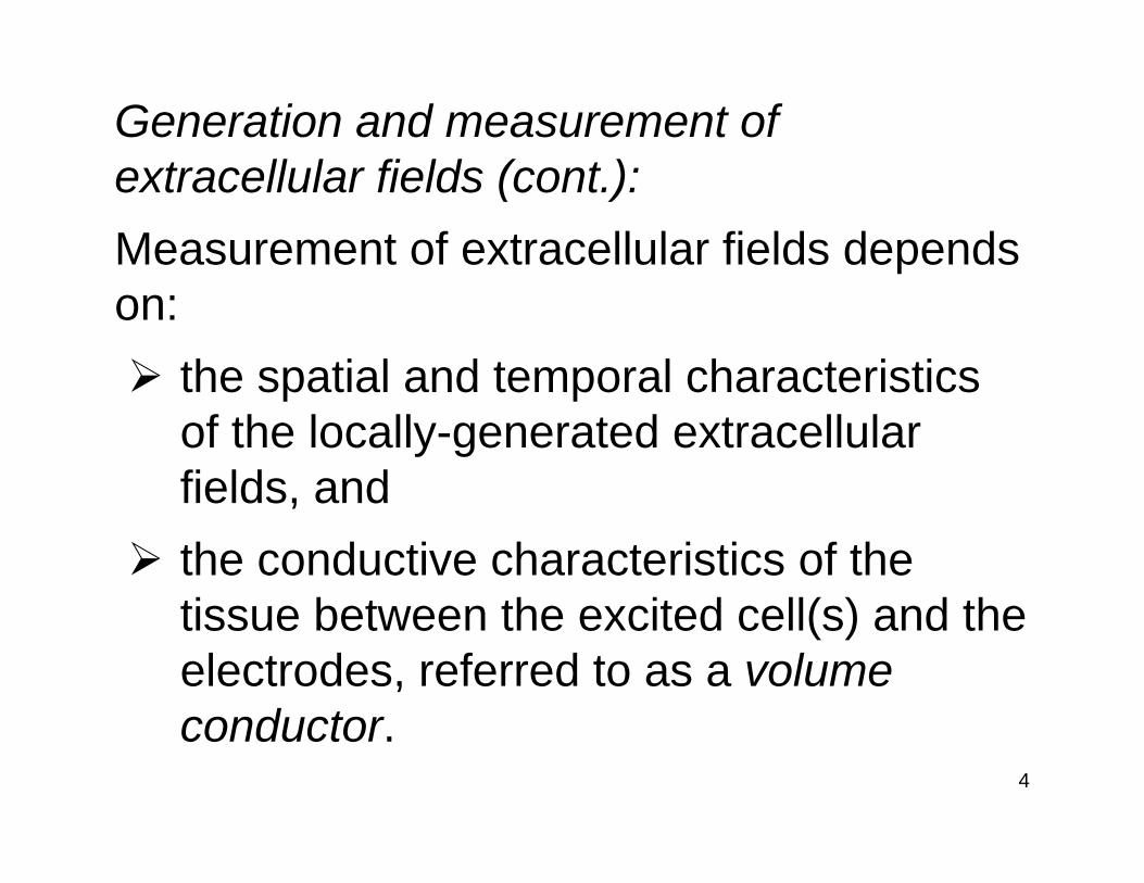
Generation and measurement of extracellular fields (cont.):Measurement of extracellular fields depends on: the spatial and temporal characteristics

of the locally-generated extracellular fields, and

the conductive characteristics of the tissue between the excited cell(s) and the electrodes, referred to as a volume conductor.

5

Observed extracellular potentials:

6

Observed extracellular potentials (cont.):The temporal waveforms of extracellular potentials cannot be determined directly from the temporal waveforms for transmembrane potentials. Instead the following steps must be taken:1. Convert transmembrane potential temporal waveform

into spatial waveform.2. Find transmembrane current and/or axial extracellular

current.3. Find extracellular spatial waveform produced by

transmembrane current (or alternatively axial extracellular current).

4. Convert extracellular spatial waveform into temporal waveform.

7

Observed extracellular potentials (cont.):

8


9

Source density im(x):The transmembrane current im(x) acts as a current source in the extracellular electrolyte.From the cable equations:

For an axon with radius a and axoplasmicresistivity Ri, Eqn. (8.3) becomes:

where σi=1/Ri is the conductance per unit length.

10

Source density im(x):However, one normally knows Vm(x) but not Φi(x).In the case where re¿ ri, Vm(x) ≈ Φi(x) and thus:

Under this approximation:

11

Source density im(x) (cont.):

12


13

Single-fiber source model:The next step is to derive mathematical expressions for the potential at any point in the extracellular space, based on the transmembrane current source model of a single fiber.

14

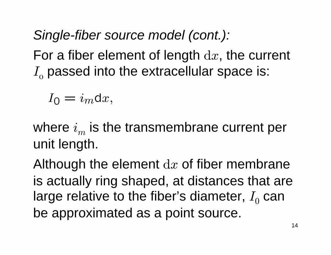
Single-fiber source model (cont.):For a fiber element of length dx, the current I0 passed into the extracellular space is:

where im is the transmembrane current per unit length.Although the element dx of fiber membrane is actually ring shaped, at distances that are large relative to the fiber’s diameter, I0 can be approximated as a point source.

15

Single-fiber source model (cont.):For a point source, the extracellular field is:

where I0 = imdx, σe is the conductivity of the extracellular medium, and r is the distance from the point source to an arbitrary field point.Note that once again the effect of the fiberon the field is typically ignored.

16

Single-fiber source model (cont.):The extracellular field for the fiber element dx is:

and the total extracellular potential at point Pis:

where L is the length of the fiber over which im 0.

17

Single-fiber source model (cont.):Substituting (8.8) into (8.11) gives:

The potential difference between two extracellular electrodes at positions a and bis then:

18

Single-fiber source model (cont.):If the element dx is located at point (x, y, z)and the field potential is measured at(x 0, y 0, z 0), then:

Normally the coordinate origin is placed on the fiber so that y = z = 0. Since the source element is approximated by a point source, it too lies on the fiber’s axis.

19

Single-fiber source model (cont.):With this expression for r, the field potential is given by:

Eqn. (8.15) can be written as the convolution:

20

Single-fiber source model (cont.):

21

Single-fiber source model (cont.):

22

Single-fiber source model (cont.):Eqn. (8.12) can be considered the integral:

of the monopole source density I` (with units of current per unit length):

23

Lumped monopole source model:For a typical action potential waveform, the monopole source density is triphasic, with the three phases each extending over a fairly short section of the fiber, as illustrated in the next slide.Consequently, these three source density regions can be approximated by three lumped monopoles M1, M2 & M3.This is readily shown by approximating the AP waveform as a triangle (see next slide).

24

Lumped monopole source model (cont.):

25

Lumped monopole source model (cont.):From Eqn. (8.19), the total monopole strength arising from the distributed monopole densities in any interval xa to xb is given by:

26

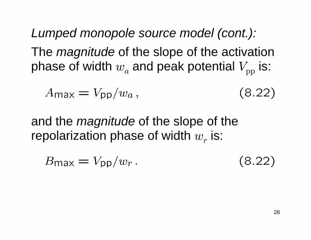
Lumped monopole source model (cont.):The magnitude of the slope of the activation phase of width wa and peak potential Vpp is:

and the magnitude of the slope of the repolarization phase of width wr is:

27

Lumped monopole source model (cont.):Consequently:

These three lumped (i.e., discrete) monopole sources are located at the activation onset, AP peak & repolarization offset and approximate the actual distributed monopole source densities.

28

Lumped monopole source model (cont.):The net extracellular field potential generated by these three sources is then:

where r1, r2 & r3 are the respective distances from the sources to the field point.

29

Lumped monopole source model (cont.):Note:-1. A lumped monopole source is a good

approximation only at a reasonable distance from the fiber.

2. Eqn. (8.21) can be used to determine three lumped monopoles directly from the AP waveform, rather than the triangular approximation. In this case, each monopole is located at the “center of gravity” of the monopole source density that it is approximating.

30

Lumped fiber source models (cont.):The spatialwaveform of anaction potentialpropagating inthe negative xdirection, andits first twospatial derivates,with the resultantsource densities.

(From Plonsey & Barr, 2nd Edition)

31

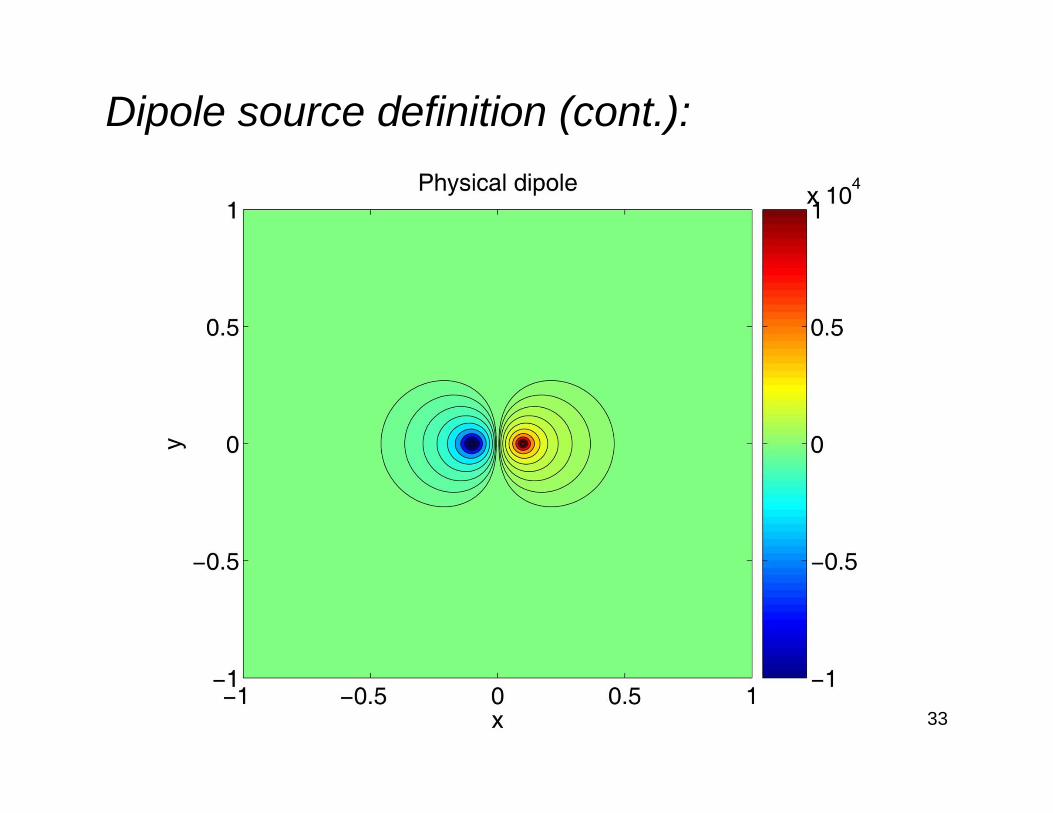
Dipole source definition:The “tripole” lumped monopole model derived in the last lecture could also be interpreted as a pair of physical dipoles, one with current strength +πa2σiAmax at the onset of activation and −πa2σiAmax at the peak of the AP, and another with current strength +πa2σiBmax at the offset of repolarization and −πa2σiBmax at the peak of the AP.

32

Dipole source definition (cont.):

33


34

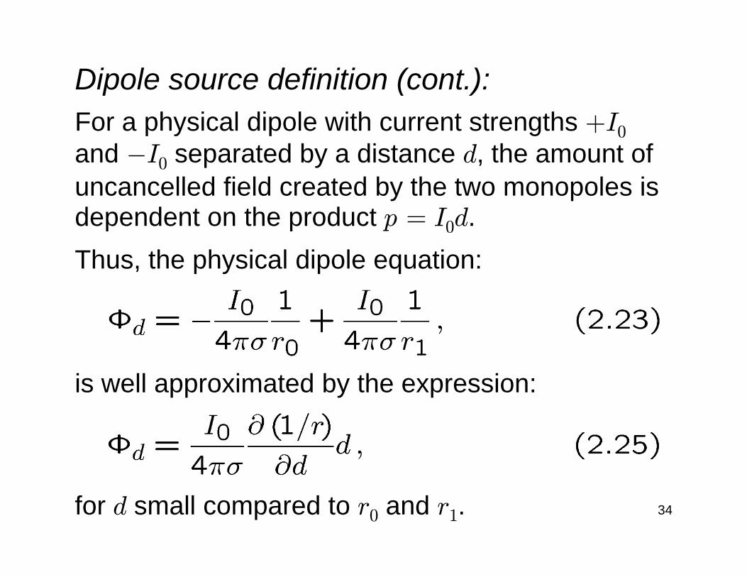
Dipole source definition (cont.):For a physical dipole with current strengths +I0and −I0 separated by a distance d, the amount of uncancelled field created by the two monopoles is dependent on the product p = I0d.Thus, the physical dipole equation:

is well approximated by the expression:

for d small compared to r0 and r1.

35

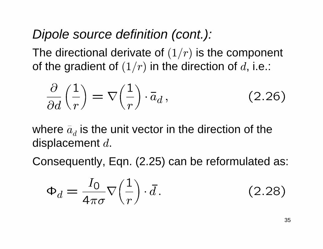
Dipole source definition (cont.):The directional derivate of (1/r) is the component of the gradient of (1/r) in the direction of d, i.e.:

where ad is the unit vector in the direction of the displacement d.Consequently, Eqn. (2.25) can be reformulated as:

—

36

Dipole source definition (cont.):An idealized or “perfect” dipole is the point source equivalent of a physical dipole. It is created by letting d→ 0 and I0→∞ such that p = I0dremains constant and finite. Eqn. (2.28) then becomes:

where the dipole vector p = pad is typically located at a point midway between the positive and negative physical dipoles sources and oriented in the direction of the positive source.

— —

37

Dipole source definition (cont.):The gradient of (1/r) can be shown to equal:

where ar is the unit vector from the dipole source location to the field point. If θ is the angle between ar and p, then:

—

— —

38


39

Single-fiber dipole source model:Eqn. (8.12) can be rewritten in the form:

Integrating by parts gives:

40

Single-fiber dipole source model (cont.):The integrated part of (8.34) is zero if the action potential is not at the ends of the fiber, and it is only necessary to integrate over the region L of the fiber where Vm/x 0, giving:

Again, the directional derivative is:

41

Single-fiber dipole source model (cont.):Substituting (8.36) into (8.35) gives:

Eqn. (8.37) can be considered the integral of the dipole source density:

with units of current (current times length per unit length) oriented in the x direction. Note the final approximation in (8.41) is true for re¿ ri.

42

Single-fiber dipole source model (cont.):The field potential generated by a dipole source density is then:

Because the first derivate of a typical AP spatial waveform is biphasic, a propagating AP produces a pair of dipole source regions, each with the dipoles pointing away from the peak of the AP.Note that these dipole source regions are consistent with the diffuse axial extracellular currents Ie produced by a propagating AP.

43

Lumped dipole source model:The two dipole source density regions can be approximated by two lumped dipoles, a dipole Dp pointing in the +ve x direction at the activation phase and a dipole Dn

pointing in the −ve x direction at the repolarization phase of an AP propagating in the +ve x direction.Note that these dipoles would be switched if the AP were propagating in the −ve xdirection.

44

Lumped dipole source model (cont.):

45

Lumped dipole source model (cont.):From Eqn. (8.41), the total dipole strength arising from the distributed dipole densities in any interval x1 to x2 is given by:

46

Lumped dipole source model (cont.):Hence, the lumped dipole strength associated with the activation interval xb to xc is:

and the lumped dipole strength for the repolarization interval xa to xb is:

47

Lumped monopole source model (cont.):Note:-1. Each lumped dipole is located at the

“center of gravity” of the dipole source density that it approximates.

2. A lumped dipole source is a good approximation only at a reasonable distance from the fiber.

3. Eqn. (8.46) can be used to determine lumped dipoles directly from the AP waveform, rather than the triangular approximation.

48

Temporal considerations:The temporal waveform of external field potentials will depend on the locations of the recording electrodes.

(from Johnstonand Wu)

49

Temporal considerations (cont.):While the action potential is propagating along an axon, it is producing a pair of dipole sources (or a quadrupole source).

However, while the action potential is being initiated (typically at the axon hillock, the patch of membrane where the axon joins the soma) and when the action potential reaches the axon terminals, only one dipole source exists.

The dendritic tree acts as a passive source during action potential initiation.

50

Temporal considerations (cont.):The dendritic tree also acts as an active sink or source due to synaptic inputs on the dendrites, with a soma forming the passive source or sink, respectively, generating a dipole source.


51

Temporal considerations (cont.):Dipole sources arealso generated inthe heart because the action potential duration is around 200—300 ms, such that the depolarization and repolarization phases are temporally separated.

52

Classification of fields:The net electrical field generated by simultaneous synaptic input in a group of neurons depends on the geometrical arrangement of the neurons.There are three typically arrangements that lead to three characteristic fields:1. the open field,2. the closed field, and3. the open-closed field.

53

Classification of fields (cont.):


54

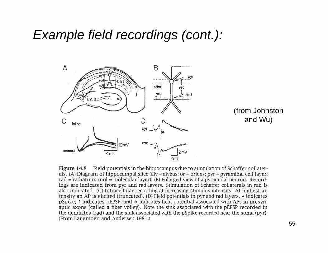
Example field recordings:Several open fields are generated within the hippocampus, where simultaneous synaptic input commonly occurs.


55

Example field recordings (cont.):


56



57



ECE795 - Lecture #6.ppt

Documents

Transcript of ECE795 - Lecture #6.ppt