ECE356S Linear Systems & Control - University of …broucke/ece356s/ece356Book2008.pdfECE356S Linear...
117
ECE356S Linear Systems & Control Bruce Francis Course notes, Version 2.0, January 2008
Transcript of ECE356S Linear Systems & Control - University of …broucke/ece356s/ece356Book2008.pdfECE356S Linear...

ECE356S Linear Systems & Control
Bruce Francis
Course notes, Version 2.0, January 2008


Preface
This is the first Engineering Science course on control. It may be your one and only course oncontrol, and therefore the aim is to give both some breadth and some depth. Mathematical modelsof mostly mechanical systems is an important component. There’s also an introduction to statemodels and state-space theory. Finally, there’s an introduction to design in the frequency domain.
The sequels to this course are ECE557 Systems Control, which develops the state-space methodin continuous time, and ECE411 Real-Time Computer Control, which treats digital control via bothstate-space and frequency-domain methods.
There are several computer applications for solving numerical problems in this course. The mostwidely used is MATLAB, but it’s expensive. I like Scilab, which is free. Others are Mathematica(expensive) and Octave (free).
3

4

Contents
1 Introduction 11.1 Problems . . . . . . . . . . . . . . . . . . . . . . . . . . . . . . . . . . . . . . . . . . 1
2 Mathematical Models of Systems 32.1 Block Diagrams . . . . . . . . . . . . . . . . . . . . . . . . . . . . . . . . . . . . . . . 32.2 State Models . . . . . . . . . . . . . . . . . . . . . . . . . . . . . . . . . . . . . . . . 52.3 Linearization . . . . . . . . . . . . . . . . . . . . . . . . . . . . . . . . . . . . . . . . 152.4 Simulation . . . . . . . . . . . . . . . . . . . . . . . . . . . . . . . . . . . . . . . . . . 182.5 The Laplace Transform . . . . . . . . . . . . . . . . . . . . . . . . . . . . . . . . . . 192.6 Transfer Functions . . . . . . . . . . . . . . . . . . . . . . . . . . . . . . . . . . . . . 272.7 Interconnections . . . . . . . . . . . . . . . . . . . . . . . . . . . . . . . . . . . . . . 302.8 Problems . . . . . . . . . . . . . . . . . . . . . . . . . . . . . . . . . . . . . . . . . . 32
3 Linear System Theory 353.1 Initial-State-Response . . . . . . . . . . . . . . . . . . . . . . . . . . . . . . . . . . . 353.2 Input-Response . . . . . . . . . . . . . . . . . . . . . . . . . . . . . . . . . . . . . . . 383.3 Total Response . . . . . . . . . . . . . . . . . . . . . . . . . . . . . . . . . . . . . . . 403.4 Logic Notation . . . . . . . . . . . . . . . . . . . . . . . . . . . . . . . . . . . . . . . 413.5 Lyapunov Stability . . . . . . . . . . . . . . . . . . . . . . . . . . . . . . . . . . . . . 443.6 BIBO Stability . . . . . . . . . . . . . . . . . . . . . . . . . . . . . . . . . . . . . . . 483.7 Frequency Response . . . . . . . . . . . . . . . . . . . . . . . . . . . . . . . . . . . . 523.8 Problems . . . . . . . . . . . . . . . . . . . . . . . . . . . . . . . . . . . . . . . . . . 54
4 Feedback Control Theory 574.1 Closing the Loop . . . . . . . . . . . . . . . . . . . . . . . . . . . . . . . . . . . . . . 574.2 The Internal Model Principle . . . . . . . . . . . . . . . . . . . . . . . . . . . . . . . 654.3 Principle of the Argument . . . . . . . . . . . . . . . . . . . . . . . . . . . . . . . . . 674.4 Nyquist Stability Criterion (1932) . . . . . . . . . . . . . . . . . . . . . . . . . . . . 694.5 Examples . . . . . . . . . . . . . . . . . . . . . . . . . . . . . . . . . . . . . . . . . . 704.6 Stability and Bode Plots . . . . . . . . . . . . . . . . . . . . . . . . . . . . . . . . . . 714.7 Problems . . . . . . . . . . . . . . . . . . . . . . . . . . . . . . . . . . . . . . . . . . 89
5 Introduction to Control Design 955.1 Loopshaping . . . . . . . . . . . . . . . . . . . . . . . . . . . . . . . . . . . . . . . . 955.2 Lag Compensation . . . . . . . . . . . . . . . . . . . . . . . . . . . . . . . . . . . . . 975.3 Lead Compensation . . . . . . . . . . . . . . . . . . . . . . . . . . . . . . . . . . . . 102
5

6 CONTENTS
5.4 Loopshaping Theory . . . . . . . . . . . . . . . . . . . . . . . . . . . . . . . . . . . . 1065.4.1 Bode’s phase formula . . . . . . . . . . . . . . . . . . . . . . . . . . . . . . . 1065.4.2 The waterbed effect . . . . . . . . . . . . . . . . . . . . . . . . . . . . . . . . 108
5.5 Problems . . . . . . . . . . . . . . . . . . . . . . . . . . . . . . . . . . . . . . . . . . 109

Chapter 1
Introduction
A familiar example of a control system is the one we all have that regulates our internal bodytemperature at 37◦ C. As we move from a warm room to the cold outdoors, our body temperatureis maintained. Other familiar examples of control systems:
• autofocus mechanism in cameras
• cruise control system in cars
• anti-lock brake system (ABS) and other traction control systems in cars
• thermostat temperature control systems.
More widely, control systems are in every manufacturing process. One very interesting applicationdomain is vehicle motion control, and maybe the best example of this is helicopter flight control.
This course is about the modeling of systems and the analysis and design of control systems.
1.1 Problems
1. List three examples of control systems not mentioned in class. Make your list as diverse aspossible.
2. Go to
http://www.modelaviation.co.uk/heli/models/hoverfly/hoverfly.htm
Imagine yourself flying the model helicopter shown. Draw the block diagram with you in theloop.
3. Imagine a wooden box of cube shape that can balance itself on one of its edges; while it’sbalanced on the edge, if you tapped it lightly it would right itself. Think of a mechatronicsystem to put inside the box to do this stabilization. Draw a schematic diagram of yourmechatronic system.
4. Historically, control systems go back at least to ancient Greek times. More recently, in 1769a feedback control system was invented by James Watt: the flyball governor for speed controlof a steam engine. Sketch the flyball governor and explain in a few sentences how it works.
1

2 CHAPTER 1. INTRODUCTION
[References: Many books on control; also, many interesting websites, for example,
http://www.uh.edu/engines/powersir.htm
Stability of this control system was studied by James Clerk Maxwell, whose equations youknow and love.]
5. The topic of vehicle formation is of current research interest. See for example
http://www.path.berkeley.edu
This is a very simple instance of such a problem.
Consider two cars that can move in a horizontal straight line. Let car #1 be the leader and car#2 the follower. The goal is for car #1 to follow a reference speed and for car #2 to maintaina specified distance behind. Discuss how this might be done. (We’ll study this example morelater.)

Chapter 2
Mathematical Models of Systems
The best (only?) way to learn this subject is bottom up—from specific examples to general theory.So we begin with mathematical models of physical systems. We mostly use mechanical examplessince their behaviour is easier to understand than, say, electromagnetic systems, because of ourexperience in the natural world. We have an intuitive understanding of Newtonian mechanics fromhaving played volleyball, skateboarded, etc.
2.1 Block Diagrams
Block diagrams are fundamental in control analysis and design. We can see how signals affect eachother.
Example 2.1.1 The simplest vehicle to control is a cart on wheels:
Brief Article
The Author
December 7, 2007
y
u
1
This is a schematic diagram, not a block diagram. Assume the cart can move only in a straightline on a flat surface. (There may be air resistance to the motion and other friction effects.) Assumea force u is applied to the cart and let y denote the position of the cart measured from a stationaryreference position. Then u and y are functions of time t and we could indicate this by u(t) and y(t).But we are careful to distinguish between u, a function, and the value u(t) of this function at timet. We regard the functions u and y as signals.
Newton’s second law tells us that there’s a mathematical relationship between u and y, namely,u = My. We take the viewpoint that the force can be applied independently of anything else, thatis, it’s an input. Then y is an output. We represent this graphically by a block diagram:
3

4 CHAPTER 2. MATHEMATICAL MODELS OF SYSTEMS
Brief Article
The Author
December 7, 2007
u y
1
So a block diagram has arrows representing signals and boxes representing system components; theboxes represent functions that map inputs to outputs. Suppose the cart starts at rest at the originat time 0, i.e., y(0) = y(0) = 0. Then the position depends only on the force applied. However y attime t depends on u not just at time t, but on past times as well. So we can write y = F (u), i.e., yis a function of u, but we can’t write y(t) = F (u(t)). 2
Block diagrams also may have summing junctions:
Brief Article
The Author
December 7, 2007
ustands for y = u + v
stands for y = u ! v
v
u
v
y
y
-
1
Also, we may need to allow a block to have more than one input:
Brief Article
The Author
December 7, 2007
u
v
y
1
This means that y is a function of u and v, y = F (u, v).
Example 2.1.2
Brief Article
The Author
December 7, 2007
on a fulcrum
d
!
"
flat board
can of soup free toroll on board
1
Suppose a torque τ is applied to the board. Let θ denote the angle of tilt and d the distance of roll.Then both θ and d are functions of τ . The block diagram could be

2.2. STATE MODELS 5
Brief Article
The Author
December 7, 2007
!
"
d
1
or
Brief Article
The Author
December 7, 2007
!
"
d
1
2.2 State Models
In control engineering, the system to be controlled is termed the plant. For example, in helicopterflight control, the plant is the helicopter itself plus its sensors and actuators. The control system isimplemented in an onboard computer. The design of a flight control system for a helicopter requiresfirst the development of a mathematical model of the helicopter dynamics. This is a very advancedsubject, well beyond the scope of this course. We must content ourselves with much simpler plants.
Example 2.2.1 Consider a cart on wheels, driven by a force F and subject to air resistance:
Brief Article
The Author
December 7, 2007
M
y
F
1
Typically air resistance creates a force depending on the velocity y; let’s say this force is a possiblynonlinear function D(y). Assuming M is constant, Newton’s second law gives
My = F −D(y).
We are going to put this in a standard form. Define what are called state variables:
x1 := y, x2 := y.

6 CHAPTER 2. MATHEMATICAL MODELS OF SYSTEMS
Then
x1 = x2
x2 =1MF − 1
MD(x2)
y = x1.
These equations have the form
x = f(x, u), y = h(x) (2.1)
where
x :=[x1
x2
], u := F
f : R2 × R→ R2, f(x1, x2, u) =
x2
1M u−
1MD(x2)
h : R2 → R, h(x1, x2) = x1.
The function f is nonlinear if D is; h is linear. Equation (2.1) constitutes a state model of thesystem, and x is called the state or state vector. The block diagram is
Brief Article
The Author
December 7, 2007
u yP
(x)
1
Here P is a possibly nonlinear system, u (applied force) is the input, y (cart position) is the output,and
x =[
cart pos’ncart velocity
]is the state of P . (We’ll define state later.)
As a special case, suppose the air resistance is a linear function of velocity:
D(x2) = D0x2, D0 a constant.
Then f is linear:
f(x, u) = Ax+Bu, A :=[
0 10 −D0/M
], B :=
[0
1/M
].
Defining C =[
0 1], we get the state model
x = Ax+Bu, y = Cx. (2.2)
This model is of a linear, time-invariant (LTI) system. 2

2.2. STATE MODELS 7
It is convenient to write vectors sometimes as column vectors and sometimes as n-tuples, i.e.,ordered lists. For example
x :=[x1
x2
], x = (x1, x2).
We shall use both.Generalizing the example, we can say that an important class of models is
x = f(x, u), f : Rn × Rm → Rn
y = h(x, u), h : Rn × Rm → Rp.
This model is nonlinear, time-invariant. The input u has dimension m, the output y dimension p,and the state x dimension n. An example where m = 2, p = 2, n = 4 is
Brief Article
The Author
December 7, 2007
y1 y2
u1
M1
u2
M2
K
1
u = (u1, u2), y = (y1, y2), x = (y1, y1, y2, y2).
The LTI special case is
x = Ax+Bu, A ∈ Rn×n, B ∈ Rn×m
y = Cx+Du, C ∈ Rp×n, D ∈ Rp×m.
Now we turn to the concept of the state of a system. Roughly speaking, x(t0) encapsulatesall the system dynamics up to time t0, that is, no additional prior information is required. Moreprecisely, the concept is this: For any t0 and t1, with t0 < t1, knowing x(t0) and knowing {u(t) :t0 ≤ t ≤ t1}, we can compute x(t1), and hence y(t1).
Example 2.2.2
Brief Article
The Author
December 7, 2007
y
M no force; no air resistance
1

8 CHAPTER 2. MATHEMATICAL MODELS OF SYSTEMS
If we were to try simply x = y, then knowing x(t0) without y(t0), we could not solve the initial valueproblem for the future cart position. Similarly x = y won’t work. Since the equation of motion,My = 0, is second order, we need two initial conditions at t = t0, implying we need a 2-dimensionalstate vector. In general for mechanical systems it is customary to take x to consist of positions andvelocities of all masses. 2
Example 2.2.3 mass-spring-damper
Brief Article
The Author
December 7, 2007
u
free-body :
Mg
y
M
K(y ! y0) D0y
u
D0K
1
My = u+Mg −K(y − y0)−D0y
state x = (x1, x2), x1 = y, x2 = y
x1 = x2
x2 =1Mu+ g − K
Mx1 +
K
My0 −
D0
Mx2
y = x1
This has the form
x = Ax+Bu+ c
y = Cx
where
A =[
0 1−KM −D0
M
], B =
[01M
], c =
[0
g + KM y0
]= const. vector
C = [1 0] .
The constant vector c is known, and hence is taken as part of the system rather thanas a signal. 2
Example 2.2.4 Active suspension
2.2. STATE MODELS 9
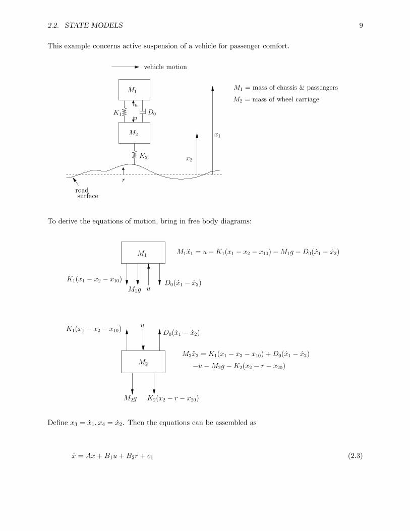
This example concerns active suspension of a vehicle for passenger comfort.
Brief Article
The Author
December 7, 2007
D0
vehicle motion
M1
M2 x1
M1 = mass of chassis & passengers
M2 = mass of wheel carriage
K1
x2
u
roadsurface
r
K2
u
1
To derive the equations of motion, bring in free body diagrams:
Brief Article
The Author
December 7, 2007
M1
M2
M2x2 = K1(x1 ! x2 ! x10) + D0(x1 ! x2)
!u ! M2g ! K2(x2 ! r ! x20)
K2(x2 ! r ! x20)
M1x1 = u ! K1(x1 ! x2 ! x10) ! M1g ! D0(x1 ! x2)
uK1(x1 ! x2 ! x10)
M1g uD0(x1 ! x2)
D0(x1 ! x2)
M2g
K1(x1 ! x2 ! x10)
1
Define x3 = x1, x4 = x2. Then the equations can be assembled as
x = Ax+B1u+B2r + c1 (2.3)

10 CHAPTER 2. MATHEMATICAL MODELS OF SYSTEMS
where
x =
x1
x2
x3
x4
, c1 =
00
K1M1x10 − g
−K1M2x20 − g + K2
M2x20
= constant vector
A =
0 0 1 0
0 0 0 1
−K1M1
K1M1
−D0M1
D0M1
K1M2
−K1+K2M2
D0M2
−D0M2
, B1 =
0
0
1M1
− 1M2
, B2 =
0
0
0
K2M2
.
We can regard (2.3) as corresponding to the block diagram
Brief Article
The Author
December 7, 2007
r(t)
u(t) x(t)P
1
Since c1 is a known constant vector, it’s not taken to be a signal. Here u(t) is the controlled inputand r(t) the uncontrolled input or disturbance.
The output to be controlled might be acceleration or jerk of the chassis. Taking y = x1 = x3
gives
y = Cx+Du+ c2 (2.4)
where
C =[−K1M1
K1M1
−D0M1
D0M1
], D =
1M1
, c2 =K1
M1x10 − g.
Equations (2.3) and (2.4) have the form
x = f(x, u, r)
y = h(x, u).
Notice that f and h are not linear, because of the constants c1, c2. 2
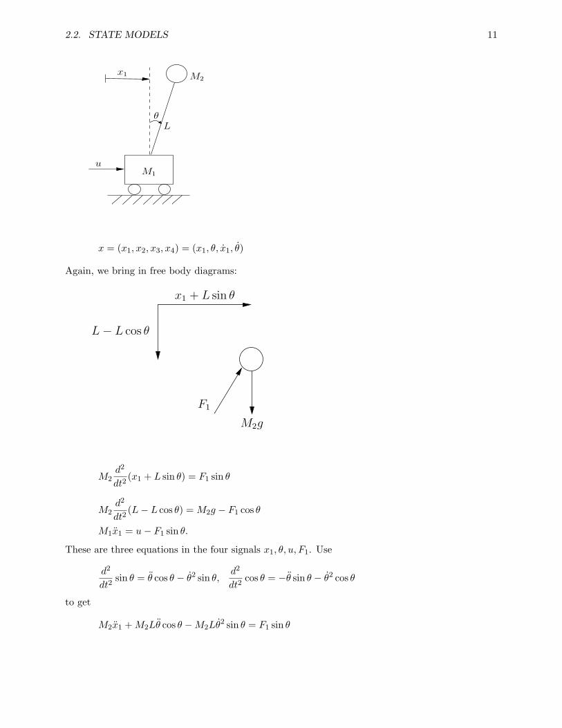
Example 2.2.5 Cart-pendulumA favourite toy control problem is to get a cart to automatically balance a pendulum.
2.2. STATE MODELS 11
Brief Article
The Author
December 7, 2007
M1
u
M2
x1
L
!
1
x = (x1, x2, x3, x4) = (x1, θ, x1, θ)
Again, we bring in free body diagrams:
Brief Article
The Author
December 7, 2007
M2g
F1
x1 + L sin !
L ! L cos !
1
M2d2
dt2(x1 + L sin θ) = F1 sin θ
M2d2
dt2(L− L cos θ) = M2g − F1 cos θ
M1x1 = u− F1 sin θ.
These are three equations in the four signals x1, θ, u, F1. Use
d2
dt2sin θ = θ cos θ − θ2 sin θ,
d2
dt2cos θ = −θ sin θ − θ2 cos θ
to get
M2x1 +M2Lθ cos θ −M2Lθ2 sin θ = F1 sin θ

12 CHAPTER 2. MATHEMATICAL MODELS OF SYSTEMS
M2Lθ sin θ +M2Lθ2 cos θ = M2g − F1 cos θ
M1x1 = u− F1 sin θ.
We can eliminate F1: Add the first and the third to get
(M1 +M2)x1 +M2Lθ cos θ −M2Lθ2 sin θ = u;
multiply the first by cos θ, the second by sin θ, add, and cancel M2 to get
x1 cos θ + Lθ − g sin θ = 0.
Solve the latter two equations for x1 and θ:[M1 +M2 M2L cos θ
cos θ L
] [x1
θ
]=[u+M2Lθ
2 sin θg sin θ
].
Thus
x1 =u+M2Lθ
2 sin θ −M2g sin θ cos θM1 +M2 sin2 θ
θ =−u cos θ −M2Lθ
2 sin θ cos θ + (M1 +M2)g sin θL(M1 +M2 sin2 θ)
.
In terms of state variables we have
x1 = x3
x2 = x4
x3 =u+M2Lx
24 sinx2 −M2g sinx2 cosx2
M1 +M2 sin2 x2
x4 =−u cosx2 −M2Lx
24 sinx2 cosx2 + (M1 +M2)g sinx2
L(M1 +M2 sin2 x2).
Again, these have the form
x = f(x, u).
We might take the output to be
y =[x1
θ
]=[x1
x2
]= h(x).
The system is highly nonlinear, though, as you would expect, it can be approximated by a linearsystem for |θ| small enough, say < 5◦. 2
Example 2.2.6 Level control

2.2. STATE MODELS 13
Brief Article
The Author
December 17, 2007
d
u
valve
x
d = flow rate in, taken to be a disturbance
u = stroke of valve
x = height of liquid in tank
1
Let A = cross-sectional area of tank, assumed constant. Then conservation of mass:
Ax = d− (flow rate out).
Also
(flow rate out) = (const)×√
∆p× (area of valve opening)
where
∆p = pressure drop across valve= (const)× x.
Thus
(flow rate out) = c√x u
and hence
Ax = d− c√x u.
The state equation is therefore
x = f(x, u, d) =1Ad− c
A
√x u.
2
It is worth noting that not all systems have state models of the form
x = f(x, u), y = h(x, u).
Examples:
1. Differentiator y = u
2. Time delay y(t) = u(t− 1)
14 CHAPTER 2. MATHEMATICAL MODELS OF SYSTEMS
3. Time-varying system
Brief Article
The Author
December 17, 2007
M(t) M a function of time (e.g. burning fuel)u
1
4. PDE model, e.g. vibrating violin string with input the bow force.
Finally, let us see how to get a state model for an electric circuit.
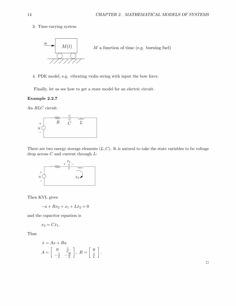
Example 2.2.7
An RLC circuit.
Brief Article
The Author
December 17, 2007
+ CR L
u!
1
There are two energy storage elements (L,C). It is natural to take the state variables to be voltagedrop across C and current through L:
Brief Article
The Author
December 17, 2007
+
u
!
x1
x2
+ !
1
Then KVL gives
−u+Rx2 + x1 + Lx2 = 0
and the capacitor equation is
x2 = Cx1.
Thus
x = Ax+Bu
A =[
0 1C
− 1L −R
L
], B =
[01L
].
2

2.3. LINEARIZATION 15
2.3 Linearization
So far we have seen that many systems can be modeled by nonlinear state equations of the form
x = f(x, u), y = h(x, u).
(There might be disturbance inputs present, but for now we suppose they are lumped into u.) Thereare techniques for controlling nonlinear systems, but that’s an advanced subject. However, manysystems can be linearized about an equilibrium point. In this section we see how to do this. Theidea is to use Taylor series.
Example 2.3.1
Let’s linearize the function y = f(x) = x3 about the point x0 = 1. The Taylor series expansion is
f(x) =∞∑0
cn(x− x0)n, cn =f (n)(x0)
n!
= f(x0) + f ′(x0)(x− x0) +f ′′(x0)
2(x− x0)2 + ... .
Taking only terms n = 0, 1 gives
f(x) ≈ f(x0) + f ′(x0)(x− x0),
that is
y − y0 ≈ f ′(x0)(x− x0).
Defining ∆y = y− y0, ∆x = x− x0, we have the linearized function ∆y = f ′(x0)∆x, or ∆y = 3∆xin this case.
Brief Article
The Author
December 17, 2007
11
1
x
y
slope = 3
!x
!y
3
1
Obviously, this approximation gets better and better as |∆x| gets smaller and smaller. 2
Taylor series extend to functions f : Rn → Rm.
Example 2.3.2

16 CHAPTER 2. MATHEMATICAL MODELS OF SYSTEMS
f : R3 → R2, f(x1, x2, x3) = (x1x2 − 1, x23 − 2x1x3)
Suppose we want to linearize f at the point x0 = (1,−1, 2). Terms n = 0, 1 in the expansion are
f(x) ≈ f(x0) +∂f
∂x(x0)(x− x0),
where
∂f
∂x(x0) = Jacobian of f at x0
=(∂fi∂xj
(x0))
=[
x2 x1 0−2x3 0 2x3 − 2x1
]∣∣∣∣x0
=[−1 1 0−4 0 2
].
Thus the linearization of y = f(x) at x0 is ∆y = A∆x, where
A =∂f
∂x(x0) =
[−1 1 0−4 0 2
]∆y = y − y0 = f(x)− f(x0)∆x = x− x0.
2
By direct extension, if f : Rn × Rm → Rn, then
f(x, u) ≈ f(x0, u0) +∂f
∂x(x0, u0)∆x+
∂f
∂u(x0, u0)∆u.
Now we turn to linearizing the differential equation
x = f(x, u).
First, assume there is an equilibrium point, that is, a constant solution x(t) ≡ x0, u(t) ≡ u0. Thisis equivalent to saying that 0 = f(x0, u0). Now consider a nearby solution:
x(t) = x0 + ∆x(t), u(t) = u0 + ∆u(t), ∆x(t),∆u(t) small.
We have
x(t) = f [x(t), u(t)]= f(x0, u0) +A∆x(t) +B∆u(t) + higher order terms
where
A :=∂f
∂x(x0, u0), B :=
∂f
∂u(x0, u0).

2.3. LINEARIZATION 17
Since x = ∆x and f(x0, u0) = 0, we have the linearized equation to be
∆x = A∆x+B∆u.
Similarly, the output equation y = h(x, u) linearizes to
∆y = C∆x+D∆u,
where
C =∂h
∂x(x0, u0), D =
∂h
∂u(x0, u0).
Summary
Linearizing x = f(x, u), y = h(x, u): Select, if one exists, an equilibrium point. Compute the fourJacobians, A,B,C,D, of f and h at the equilibrium point. Then the linearized system is
∆x = A∆x+B∆u, ∆y = C∆x+D∆u.
Under mild conditions (sufficient smoothness of f and h), this linearized system is a valid approxi-mation of the nonlinear one in a sufficiently small neighbourhood of the equilibrium point.
Example 2.3.3
x = f(x, u) = x+ u+ 1y = h(x, u) = x
An equilibrium point is composed of constants x0, u0 such that
x0 + u0 + 1 = 0.
So either x0 or u0 must be specified, that is, the analyst must select where the linearization is tobe done. Let’s say x0 = 0. Then u0 = −1 and
A = 1, B = 1, C = 1, D = 0.
Actually, here A,B,C,D are independent of x0, u0, that is, we get the same linear system at everyequilibrium point. 2
Example 2.3.4 Cart-pendulum
See f(x, u) in Example 2.2.5. An equilibrium point
x0 = (x10, x20, x30, x40), u0
satisfies f(x0, u0) = 0, i.e.,
x30 = 0
x40 = 0
u0 +M2Lx240 sinx20 −M2g sinx20 cosx20 = 0

18 CHAPTER 2. MATHEMATICAL MODELS OF SYSTEMS
−u0 cosx20 −M2Lx240 sinx20 cosx20 + (M1 +M2)g sinx20 = 0.
Multiply the third equation by cosx20 and add to the fourth: We get in sequence
−M2g sinx20 cos2 x20 + (M1 +M2)g sinx20 = 0
(sinx20)(M1 +M2 sin2 x20) = 0
sinx20 = 0
x20 = 0 or π.
Thus the equilibrium points are described by
x0 = (arbitrary, 0 or π, 0, 0), u0 = 0.
We have to choose x20 = 0 (pendulum up) or x20 = π (pendulum down). Let’s take x20 = 0. Thenthe Jacobians compute to
A =
0 0 1 0
0 0 0 1
0 −M2M1g 0 0
0 M1+M2M1
gL 0 0
, B =
0
01M1
− 1LM1
.
The above provides a general method of linearizing. In this particular example, there’s a fasterway, which is to approximate sin θ = θ, cos θ = 1 in the original equations:
M2d2
dt2(x1 + Lθ) = F1θ
0 = M2g − F1
M1x1 = u− F1θ.
These equations are already linear and lead to the above A and B. 2
2.4 Simulation
Concerning the model
x = f(x, u), y = h(x, u),
simulation involves numerically computing x(t) and y(t) given an initial state x(0) and an inputu(t). If the model is nonlinear, simulation requires an ODE solver, based on, for example, theRunge-Kutta method. Scilab and MATLAB have ODE solvers and also very nice simulation GUIs,Scicos and SIMULINK, respectively.

2.5. THE LAPLACE TRANSFORM 19
2.5 The Laplace Transform
You already had a treatment of Laplace transforms, for example, in a differential equations or circuittheory course. Nevertheless, we give a brief review here.
Let f(t) be a real-valued function defined for t ≥ 0. Its Laplace transform (LT) is
F (s) =
∞∫0
f(t)e−stdt.
Here s is a complex variable. Normally, the integral converges for some values of s and not forothers. That is, there is a region of convergence (ROC). It turns out that the ROC is always anopen right half-plane, of the form {s : Re s > a}. Then F (s) is a complex-valued function of s.
Example 2.5.1 the unit step or unit constant
f(t) ={
1 , t ≥ 00 , t < 0
F (s) =
∞∫0
e−stdt = −e−st
s
∣∣∣∣∞0
=1s
ROC : Re s > 0
The same F (s) is obtained if f(t) = 1 for all t, even t < 0. This is because the LT is oblivious tonegative time. Notice that F (s) has a pole at s = 0 on the western boundary of the ROC. 2
Example 2.5.2
f(t) = eat, F (s) =1
s− a, ROC : Re s > a
2
Example 2.5.3 sinusoid
f(t) = coswt =12(ejwt + e−jwt
)F (s) =
s
s2 + w2, ROC : Re s > 0
2
It is a theorem that f(t) has a LT provided
1. it is piecewise continuous on t ≥ 0
2. it is of exponential order, meaning there exist constants M, c such that |f(t)| ≤ Mect for allt ≥ 0.
The LT thus maps a class of time-domain functions f(t) into a class of complex-valued functionsF (s). The mapping f(t) 7→ F (s) is linear.
20 CHAPTER 2. MATHEMATICAL MODELS OF SYSTEMS
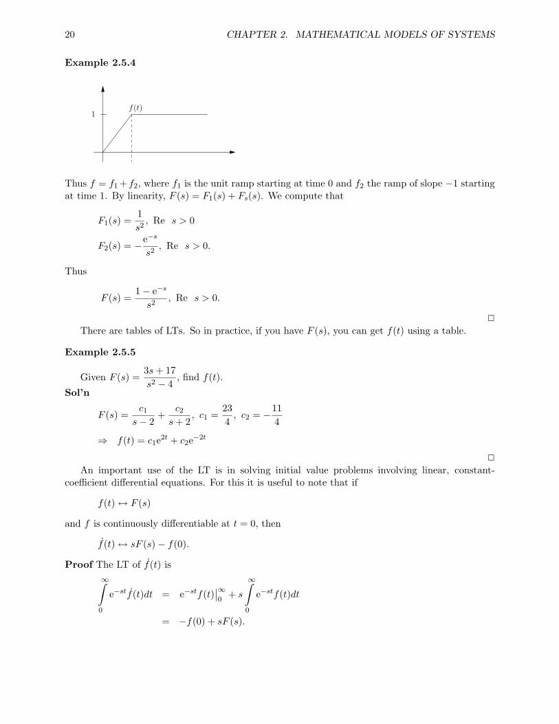
Example 2.5.4
Brief Article
The Author
December 17, 2007
f(t)1
1
Thus f = f1 +f2, where f1 is the unit ramp starting at time 0 and f2 the ramp of slope −1 startingat time 1. By linearity, F (s) = F1(s) + Fs(s). We compute that
F1(s) =1s2, Re s > 0
F2(s) = −e−s
s2, Re s > 0.
Thus
F (s) =1− e−s
s2, Re s > 0.
2
There are tables of LTs. So in practice, if you have F (s), you can get f(t) using a table.
Example 2.5.5
Given F (s) =3s+ 17s2 − 4
, find f(t).
Sol’n
F (s) =c1
s− 2+
c2
s+ 2, c1 =
234, c2 = −11
4
⇒ f(t) = c1e2t + c2e−2t
2
An important use of the LT is in solving initial value problems involving linear, constant-coefficient differential equations. For this it is useful to note that if
f(t)↔ F (s)
and f is continuously differentiable at t = 0, then
f(t)↔ sF (s)− f(0).
Proof The LT of f(t) is∞∫
0
e−stf(t)dt = e−stf(t)∣∣∞0
+ s
∞∫0
e−stf(t)dt
= −f(0) + sF (s).
2.5. THE LAPLACE TRANSFORM 21
2
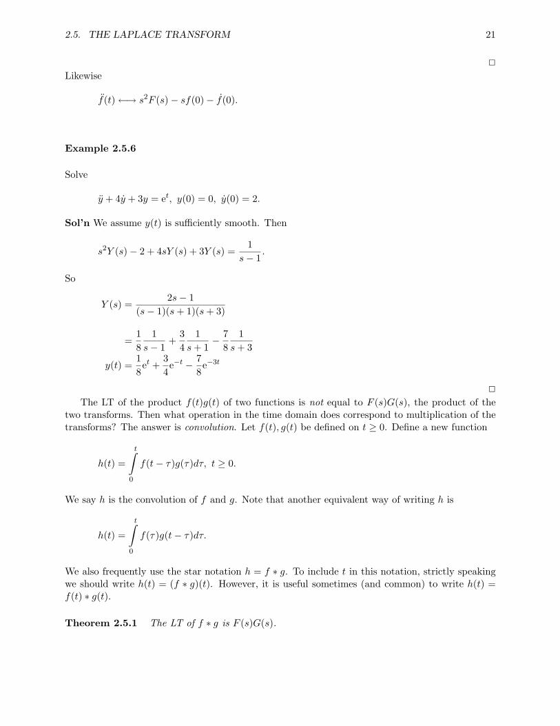
Likewise
f(t)←→ s2F (s)− sf(0)− f(0).
Example 2.5.6
Solve
y + 4y + 3y = et, y(0) = 0, y(0) = 2.
Sol’n We assume y(t) is sufficiently smooth. Then
s2Y (s)− 2 + 4sY (s) + 3Y (s) =1
s− 1.
So
Y (s) =2s− 1
(s− 1)(s+ 1)(s+ 3)
=18
1s− 1
+34
1s+ 1
− 78
1s+ 3
y(t) =18
et +34
e−t − 78
e−3t
2
The LT of the product f(t)g(t) of two functions is not equal to F (s)G(s), the product of thetwo transforms. Then what operation in the time domain does correspond to multiplication of thetransforms? The answer is convolution. Let f(t), g(t) be defined on t ≥ 0. Define a new function
h(t) =
t∫0
f(t− τ)g(τ)dτ, t ≥ 0.
We say h is the convolution of f and g. Note that another equivalent way of writing h is
h(t) =
t∫0
f(τ)g(t− τ)dτ.
We also frequently use the star notation h = f ∗ g. To include t in this notation, strictly speakingwe should write h(t) = (f ∗ g)(t). However, it is useful sometimes (and common) to write h(t) =f(t) ∗ g(t).
Theorem 2.5.1 The LT of f ∗ g is F (s)G(s).

22 CHAPTER 2. MATHEMATICAL MODELS OF SYSTEMS
Proof Let h := f ∗ g. Then
H(s) =
∞∫0
h(t)e−stdt
=
∞∫0
t∫0
f(t− τ)g(τ)e−stdτdt
=
∞∫0
∞∫τ
f(t− τ)g(τ)e−stdtdτ
=
∞∫0
∞∫τ
f(t− τ)e−stdt
︸ ︷︷ ︸
(r=t−τ)
g(τ)dτ
∞∫0
f(r)e−srdre−sτ
= F (s)G(s).
2
Example 2.5.7
Consider
My +Ky = u
and suppose y(0) = y(0) = 0. Then
Ms2Y (s) +KY (s) = U(s),
So
Y (s) = G(s)U(s),
where
G(s) =1
Ms2 +K.
This function, G(s), is called the transfer function of the system with input u and output y. Thetime-domain relationship is y = g ∗ u, where g(t) is the inverse LT (ILT) of G(s). Specifically,
G(s) =1
Ms2 +K←→ g(t) =
1√MK
sin
√K
Mt (t ≥ 0).
2

2.5. THE LAPLACE TRANSFORM 23
Now we pause to discuss the problematical object, the impulse δ(t). Let us first admit that itis not a function R −→ R, because its “value” at t = 0 is not a real number. Yet the impulse is souseful in applications that we have to make it legitimate. Actually, mathematicians have workedout a very nice, consistent way of dealing with the impulse. We shall borrow the main idea: δ(t) isnot a function, but rather it is a way of defining the mapping f 7→ f(0) that maps a signal to itsvalue at t = 0. This mapping is usually written like this:∫
f(t)δ(t)dt = f(0).
That is, we pretend δ is a function that has this so-called sifting property. In particular, if we letf(t) = e−st, we get that the LT of δ is 1. Needless to say, we have to be careful with δ; for example,there’s no way to make sense of δ2. As long as δ is used in the sifting formula, we’re on safe ground.
The formula y = g∗u is the time-domain relationship between u and y that is valid for any u. Inparticular, if u(t) = δ(t), the unit impulse, then y(t) = g(t), so Y (s) = G(s). Thus we see the truemeaning of g(t): It’s the output when the input is the unit impulse and all the initial conditionsare zero. We call g(t) the impulse-response function, or the impulse response.
Example 2.5.8
Consider an RC lowpass filter with transfer function
G(s) =1
RCs+ 1.
The impulse response function is
g(t) =1
RCe−
tRC (t ≥ 0).
Now the highpass filter:
G(s) =RCs
RCs+ 1= 1− 1
RCs+ 1
g(t) = δ(t)− 1RC
e−t/RC (t ≥ 0).
2
Inversion
As was mentioned before, in practice to go from F (s) to f(t) one uses a LT table. However, for adeeper understanding of the theory, one should know that there is a mathematical form of the ILT.Let
f(t)←→ F (s)
be a LT pair and let Re s > a be the ROC. Let σ be any real number > a. Then the vertical line
{s : Re s = σ}
24 CHAPTER 2. MATHEMATICAL MODELS OF SYSTEMS
is in the ROC. The ILT formula is this:
f(t) =1
2πj
σ+j∞∫σ−j∞
estF (s)ds.
Note that the integral is a line integral up the vertical line just mentioned.This suggests a lovely application of Cauchy’s residue theorem. Suppose F (s) has the form
F (s) =polynomial of degree < n
polynomial of degree = n.
For example
F (s) =1
Ms2 +K, n = 2
F (s) =1
RCs+ 1, n = 1
but not
F (s) =RCs
RCs+ 1.
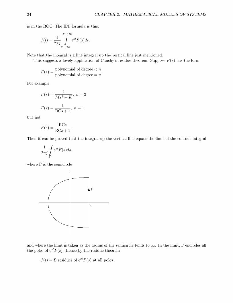
Then it can be proved that the integral up the vertical line equals the limit of the contour integral
12πj
∮Γ
estF (s)ds,
where Γ is the semicircle
Brief Article
The Author
December 17, 2007
!
!
1
and where the limit is taken as the radius of the semicircle tends to ∞. In the limit, Γ encircles allthe poles of estF (s). Hence by the residue theorem
f(t) = Σ residues of estF (s) at all poles.

2.5. THE LAPLACE TRANSFORM 25
Let us review residues.
Example
F (s) =1
s+ 1
This function has a pole at s = −1. At all other points it’s perfectly well defined. For example,near s = 0 it has a Taylor series expansion:
F (s) = F (0) + F ′(0)s+12F ′′(0)s2 + · · · =
∞∑k=0
1k!F (k)(0)sk.
Near s = 1 it has a different Taylor series expansion:
F (s) = F (1) + F ′(1)(s− 1) +12F ′′(1)(s− 1)2 + · · · =
∞∑k=0
1k!F (k)(1)(s− 1)k.
And so on. Only at s = −1 does it not have a Taylor series. Instead, it has a Laurent seriesexpansion, where we have to take negative indices:
F (s) =∞∑
k=−∞ck(s+ 1)k.
In fact, equating
1s+ 1
=∞∑
k=−∞ck(s+ 1)k
and matching coefficients, we see that ck = 0 for all k except c−1 = 1. The coefficient c−1 is calledthe residue of F (s) at the pole s = −1. 2
Example
F (s) =1
s(s+ 1)
This has a pole at s = 0 and another at s = −1. At all points except these two, F (s) has a Taylorseries. The Laurent series at s = 0 has the form
F (s) =∞∑
k=−∞cks
k.
To determine these coefficients, first do a partial-fraction expansion:
F (s) =1
s(s+ 1)=
1s− 1s+ 1
.
Then do a Taylor series expansion at s = 0 of the second term:
F (s) =1s− 1 + s+ · · · .

26 CHAPTER 2. MATHEMATICAL MODELS OF SYSTEMS
Thus the residue of F (s) at s = 0 is c−1 := 1. Similarly, to get the residue at the pole s = −1, startwith
F (s) =1s− 1s+ 1
but now do a Taylor series expansion at s = −1 of the first term:
F (s) = − 1s+ 1
− 1− (s+ 1)− (s+ 1)2 − · · · .
Thus the residue of F (s) at s = −1 is c−1 := −1. 2
More generally, if p is a simple pole of F (s), then the residue equals
lims→p
(s− p)F (s).
Example
F (s) =1
s2(s+ 1)
This has a pole at s = 0 of multiplicity 2 and a simple pole at s = −1. Partial-fraction expansionlooks like
F (s) =1
s2(s+ 1)=A
s2+B
s+
C
s+ 1.
We can get A and C by the usual coverup method, e.g.,
A = s2F (s)∣∣s=0
= 1.
The formula for B is
B =d
ds
(s2F (s)
)∣∣∣∣s=0
= −1.
Thus for this function, the residue at the pole s = 0 is B = −1. 2
Back to the ILT via residues:
f(t) =∑
residues of F (s)est at all its poles, t ≥ 0.
Example: F (s) = 1s(s−1) has two poles and est has none; thus for t ≥ 0
f(t) = Ress=01
s(s− 1)est + Ress=1
1s(s− 1)
est = −1 + et.

2.6. TRANSFER FUNCTIONS 27
2.6 Transfer Functions
Linear time-invariant (LTI) systems, and only LTI systems, have transfer functions.
Example 2.6.1 RC filter
Brief Article
The Author
December 17, 2007
u
+
!
C
R
+
!
yi
1
Circuit equations:
−u+Ri+ y = 0, i = Cdy
dt
⇒ RCy + y = u
Apply Laplace transforms with zero initial conditions:
RCY (s) + Y (s) = U(s)
⇒ Y (s)U(s)
=1
RCs+ 1=: transfer function.
Or, by voltage-divider rule using impedances:
Y (s)U(s)
=1Cs
R+ 1Cs
=1
RCs+ 1.
This transfer function is rational, a ratio of polynomials. 2
Example 2.6.2 mass-spring-damper
My = u−Ky −Dy
⇒ Y (s)U(s)
=1
Ms2 +Ds+K
This transfer function also is rational. 2
Let’s look at some other transfer functions:

28 CHAPTER 2. MATHEMATICAL MODELS OF SYSTEMS
G(s) = 1, a pure gain
G(s) =1s
, integrator
G(s) = 1s2
, double integrator
G(s) = s, differentiator
G(s) = e−τs(τ > 0), time delay; not rational
G(s) =w2n
s2 + 2ζwns+ w2n
(wn > 0, ζ ≥ 0), standard 2nd - order system
G(s) = K1 +K2
s+K3s, proportional-integral-derivative (PID) controller
We say a transfer function G(s) is proper if the degree of the denominator ≥ that of the
numerator. The transfer functions G(s) = 1,1
s+ 1are proper, G(s) = s is not. We say G(s) is
strictly proper if the degree of the denominator > that of the numerator. Note that if G(s) isproper then lim|s|→∞G(s) exists; if strictly proper then lim|s|→∞G(s) = 0. These concepts extendto multi-input, multi-output systems, where the transfer function is a matrix.
Let’s see what the transfer function is of an LTI state model:
x = Ax+Bu, y = Cx+Du
sX(s) = AX(s) +BU(s), Y (s) = CX(s) +DU(s)
⇒ X(s) = (sI −A)−1BU(s)
Y (s) = [C(sI −A)−1B +D]U(s).
We conclude that the transfer function from u to x is (sI −A)−1B and from u to y is
C(sI −A)−1B +D.
Example 2.6.3
Two carts, one spring:
A =
0 0 1 00 0 0 1−1 1 0 0
1 −1 0 0
, B =
0 00 01 00 1
C =
[1 0 0 00 1 0 0
], D =
[0 00 0
]
C(sI −A)−1B +D =
s2 + 1
s2(s2 + 2)1
s2(s2 + 2)1
s2(s2 + 2)s2 + 1
s2(s2 + 2)
.2
Let us recap our procedure for getting the transfer function of a system:

2.6. TRANSFER FUNCTIONS 29
1. Apply the laws of physics etc. to get differential equations governing the behaviour of thesystem. Put these equations in state form. In general these are nonlinear.
2. Linearize about an equilibrium point.
3. Take Laplace transforms with zero initial state.
The transfer function from input to output satisfies
Y (s) = G(s)U(s).
In general G(s) is a matrix: If dim u = m and dim y = p (m inputs, p outputs), then G(s) is p×m.In the SISO case, G(s) is a scalar-valued transfer function.
There is a converse problem: Given a transfer function, find a corresponding state model. Thatis, given G(s), find A,B,C,D such that
G(s) = C(sI −A)−1B +D.
The state matrices are never unique: Each G(s) has an infinite number of state models. But it is afact that every proper, rational G(s) has a state realization. Let’s see how to do this in the SISOcase, where G(s) is 1× 1.
Example 2.6.4 G(s) =1
2s2 − s+ 3
The corresponding differential equation model is
2y − y + 3y = u.
Taking x1 = y, x2 = y, we get
x1 = x2
x2 =12x2 −
32x1 +
12u
y = x1
and thus
A =[
0 1−3/2 1/2
], B =
[0
1/2
]C =
[1 0
], D = 0.
This technique extends to
G(s) =1
poly of degree n.
2
Example 2.6.5
G(s) =s− 2
2s2 − s+ 3

30 CHAPTER 2. MATHEMATICAL MODELS OF SYSTEMS
Introduce an auxiliary signal V (s):
Y (s) = (s− 2)1
2s2 − s+ 3U(s)︸ ︷︷ ︸
=:V (s)
Then
2v − v + 3v = u
y = v − 2v.
Defining
x1 = v, x2 = v,
we get
x1 = x2
x2 =12x2 −
32x1 +
12u
y = x2 − 2x1
and so
A =[
0 1−3/2 1/2
], B =
[01
]C =
[−2 1
], D = 0.
This extends to any strictly proper rational function. 2
Finally, if G(s) is proper but not strictly proper (deg num = deg denom), then we can write
G(s) = c+G1(s),
c = constant, G1(s) strictly proper. In this case we get A,B,C to realize G1(s), and D = c.
2.7 Interconnections
Frequently, a system is made up of components connected together in some topology. This raisesthe question, if we have state models for components, how can we assemble them into a state modelfor the overall system?
Example 2.7.1 series connection
A1 B1
C1 D1
A2 B2
C2 D2
u y1 y

2.7. INTERCONNECTIONS 31
This diagram stands for the equations
x1 = A1x1 +B1u
y1 = C1x1 +D1u
x2 = A2x2 +B2y1
y = C2x2 +D2y1.
Let us take the overall state to be
x =[x1
x2
].
Then
x = Ax+Bu, y = Cx+Du,
where
A =[
A1 0B2C1 A2
], B =
[B1
B2D1
]C =
[D2C1 C2
], D = D2D1.
2
Parallel connection
A1 B1
C1 D1
A2 B2
C2 D2
u
y1
y
y2
is very similar and is left for you.
Example 2.7.2 feedback connection
A1 B1
C1 D1
A2 B2
C2 D2
u y
!
r e
x1 = A1x1 +B1e = A1x1 +B1(r − C2x2)x2 = A2x2 +B2u = A2x2 +B2(C1x1 +D1(r − C2x2))y = C2x2

32 CHAPTER 2. MATHEMATICAL MODELS OF SYSTEMS
Taking
x =[x1
x2
]we get
x = Ax+Br, y = Cx
where
A =[
A1 −B1C2
B2C1 A2 −B2D1C2
], B =
[B1
B2D1
]C =
[0 C2
].
2
2.8 Problems
1. Consider the following system with two carts and a dashpot:
M1 M2
x1 x2
D
(Recall that a dashpot is like a spring except the force is proportional to the derivative ofthe change in length; D is the proportionality constant.) The input is the force u and thepositions of the carts are x1, x2. The other state variables are x3 = x1, x4 = x2. Take M1 = 1,M2 = 1/2, D = 1. Derive the matrices A,B in the state model x = Ax+Bu,
2. This problem concerns a beam balanced on a fulcrum. The angle of tilt of the beam is denotedα(t); a torque, denoted τ(t), is applied to the beam; finally, a ball rolls on the beam at distanced(t) from the fulcrum.
Introduce the parameters
J moment of inertia of the beamJb moment of inertia of the ballR radius of the ballM mass of the ball.
The equations of motion are given to you as(JbR2
+M
)d+Mg sinα−Mdα2 = 0
(Md2 + J + Jb)α+ 2Mddα+Mgd cosα = τ.
Put this into the form of a nonlinear state model with input τ .

2.8. PROBLEMS 33
3. Continue with the same ball-and-beam problem. Find all equilibrium points. Linearize thestate equation about the equilibrium point where α = d = 0.
4. Let A be an n× n real matrix and b ∈ Rn. Define the function
f(x) = xTAx+ bTx f : Rn −→ R,
where T denotes transpose. Linearize the equation y = f(x) at the point x0.
5. Linearize the water-tank example.
6. Consider the following feedback control system:
tan−1- j - -- - -
6
u e v x1 x2
−
The nonlinearity is the saturating function v = tan−1(e), and the two blank blocks are inte-grators modeled by
x1 = v, x2 = x1.
Taking these state variables, derive the nonlinear state equation
x = f(x, u).
Linearize the system about the equilibrium point where u = 1 and find the matrices A and Bin the linear equation
∆x = A∆x+B∆u.
[Hint:d
dytan−1 y = cos2(tan−1 y).]
7. Sketch the function
f(t) ={t+ 1, 0 ≤ t ≤ 10−2et, t > 10
and find its Laplace transform, including the region of convergence.
8. (a) Find the inverse Laplace transform of G(s) =1
2s2 + 1using the residue formula.
(b) Repeat for G(s) =1s2
.
(c) Repeat for G(s) =s2
2s2 + 1. [Hint: Write G(s) = c+G1(s) with G1(s) strictly proper.]
9. Explain why we don’t use Laplace transforms to solve the initial value problem
y(t) + 2ty(t)− y(t) = 1, y(0) = 0, y(0) = 1.

34 CHAPTER 2. MATHEMATICAL MODELS OF SYSTEMS
10. Consider a mass-spring system where M(t) is a known function of time. The equation ofmotion in terms of force input u and position output y is
d
dtMy = u−Ky
(i.e., rate of change of momentum equals sum of forces), or equivalently
My + My +Ky = u.
This equation has time-dependent coefficients. So there’s no transfer function G(s), hence noimpulse-response function g(t), hence no convolution equation y = g ? u.
(a) Find a linear state model.
(b) Guess what the correct form of the time-domain integral equation is. [Hint: If M isconstant, the output y at time t when the input is an impulse applied at time t0 dependsonly on the difference t − t0. But if M is not constant, it depends on both t and t0separately.]
11. Consider Problem 1. Find the transfer function from u to x1. Do it both by hand (from thestate model) and by Scilab or MATLAB.
12. Find a state model (A,B,C,D) for the system with transfer function
G(s) =−2s2 + s+ 1s2 − s− 4
.
13. Consider the parallel connection of G1 and G2, the LTI systems with transfer functions
G1(s) =10
s2 + s+ 1, G2(s) =
10.1s+ 1
.
(a) Find state models for G1 and G2.
(b) Find a state model for the overall system.

Chapter 3
Linear System Theory
In the preceding chapter we saw nonlinear state models and how to linearize them about an equi-librium point. The linearized systems have the form (dropping ∆)
x = Ax+Bu, y = Cx+Du.
In this chapter we study such models.
3.1 Initial-State-Response
Let us begin with the state equation forced only by the initial state—the input is set to zero:
x = Ax, x(0) = x0, A ∈ Rn×n.
Recall two facts:
1. If n = 1, i.e., A is a scalar, the unique solution of the initial-value problem is x(t) = eAtx0.
2. The Taylor series of the function et at t = 0 is
et = 1 + t+t2
2!+ · · ·
and this converges for every t. Thus
eAt = 1 +At+A2t2
2!+ · · · .
This second fact suggests that in the matrix case we define the matrix exponential eA to be
eA := I +A+12!A2 +
13!A3 + · · · .
It can be proved that the right-hand series converges for every matrix A. If A is n× n, so is eA; eA
is not defined if A is not square.
Example 3.1.1
35

36 CHAPTER 3. LINEAR SYSTEM THEORY
A =[
0 00 0
], eA =
[1 00 1
]Notice that eA is not obtained by exponentiating A componentwise. 2
Example 3.1.2
A =[
1 00 1
], eA =
[e 00 e
]= eI
2
Example 3.1.3
A =
0 1 00 0 10 0 0
This matrix has the property that A3 = 0. Thus the power series has only finitely many nonzeroterms:
eA = I +A+12A2 =
1 1 12
0 1 10 0 1
This is an example of a nilpotent matrix. That is, Ak = 0 for some power k. 2
Replacing A by At (the product of A with the scalar t) gives the matrix-valued function eAt,
t 7−→ eAt : R −→ Rn×n,
defined by
eAt = I +At+A2 t2
2!+ · · · .
This function is called the transition matrix.Some properties of eAt:
1. eAt∣∣t=0
= I
2. eAt1eAt2 = eA(t1+t2)
Note that eA1eA2 = eA1+A2 if and only if A1 and A2 commute, i.e., A1A2 = A2A1.
3. (eA)−1 = e−A, so (eAt)−1 = e−At
4. A, eAt commute
5.d
dteAt = AeAt
Now the main result:

3.1. INITIAL-STATE-RESPONSE 37
Theorem 3.1.1 The unique solution of the initial-value problem x = Ax, x(0) = x0, is x(t) = eAtx0.
This leaves us with the question of how to compute eAt. For hand calculations on small problems(n = 2 or 3), it’s convenient to use Laplace transforms.
Example 3.1.4
A =
0 1 00 0 10 0 0
, eAt =
1 t t2
20 1 t0 0 1
The Laplace transform of eAt is therefore 1/s 1/s2 1/s3
0 1/s 1/s2
0 0 1/s
.On the other hand,
(sI −A)−1 =
s −1 00 s −10 0 s
−1
=1s3
s2 s 10 s2 s0 0 s2
.We conclude that in this example eAt, (sI − A)−1 are Laplace transform pairs. This is true ingeneral. 2
If A is n× n, eAt is an n× n matrix function of t and (sI −A)−1 is an n× n matrix of rationalfunctions of s.
Example 3.1.5
A =[
0 1−1 0
](sI −A)−1 =
[s −11 s
]−1
=1
s2 + 1
[s 1−1 s
]=⇒ eAt =
[cos t sin t− sin t cos t
]2
Another way to compute eAt is via eigenvalues and eigenvectors. Instead of a general treatment,let’s do two examples.
Example 3.1.6
A =[
0 1−2 −3
]
38 CHAPTER 3. LINEAR SYSTEM THEORY
The MATLAB command [V,D] = eig (A) produces
V =[
1 −1−1 2
], D =
[−1 0
0 −2
].
The eigenvalues of A appear on the diagonal of the (always diagonal) matrix D, and the columnsof V are corresponding eigenvectors. So for example
A
[1−1
]= −1
[1−1
].
It follows that AV = V D (check this) and then that eAtV = V eDt (prove this). The nice thing isthat eDt is trivial to determine because D is diagonal. In this case
eDt =[
e−t 00 e−2t
].
Then
eAt = V eDtV −1.
2
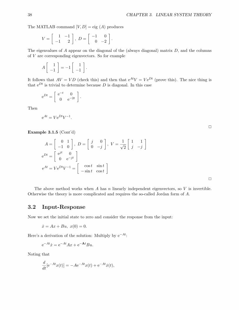
Example 3.1.5 (Cont’d)
A =[
0 1−1 0
], D =
[j 00 −j
], V =
1√2
[1 1j −j
]eDt =
[ejt 00 e−jt
]eAt = V eDtV −1 =
[cos t sin t− sin t cos t
]2
The above method works when A has n linearly independent eigenvectors, so V is invertible.Otherwise the theory is more complicated and requires the so-called Jordan form of A.
3.2 Input-Response
Now we set the initial state to zero and consider the response from the input:
x = Ax+Bu, x(0) = 0.
Here’s a derivation of the solution: Multiply by e−At:
e−Atx = e−AtAx+ e−AtBu.
Noting that
d
dt[e−Atx(t)] = −Ae−Atx(t) + e−Atx(t),
3.2. INPUT-RESPONSE 39
we get
d
dt[e−Atx(t)] = e−AtBu(t).
Integrate from 0 to t:
−eAtx(t)− x(0)︸︷︷︸=0
=
t∫0
e−AτBu(τ)dτ.
Multiply by eAt:
x(t) =
t∫0
eA(t−τ)Bu(τ)dτ. (3.1)
Equation (3.1) gives the state at time t in terms of u(τ), 0 ≤ τ ≤ t, when the initial state equalszero.
Similarly, the output equation y = Cx+Du leads to
y(t) =
t∫0
CeA(t−τ)Bu(τ)dτ +Du(t).
Special case Suppose dim u = dim y = 1, i.e., the system is single-input, single-output (SISO).Then D = D, a scalar, and we have
y(t) =
t∫0
CeA(t−τ)Bu(τ)dτ +Du(t). (3.2)
If u = δ, the unit impulse, then
y(t) = CeAtB1+(t) +Dδ(t),
where 1+(t) denotes the unit step,
1+(t) ={
1 , t ≥ 00 , t < 0.
We conclude that the impulse response of the system is
g(t) := CeAtB1+(t) +Dδ(t) (3.3)
and equation (3.2) is a convolution equation:
y(t) = (g ∗ u)(t).
Example 3.2.1

40 CHAPTER 3. LINEAR SYSTEM THEORY
y + y = u
Take the state to be
x =[x1
x2
]:=[yy
].
Then
A =[
0 10 −1
], B =
[01
]C = [ 1 0 ], D = 0.
The transition matrix:
(sI −A)−1 =
1s
1s(s+ 1)
01
s+ 1
eAt =
[1 1− e−t
0 e−t
], t ≥ 0.
Impulse response:
g(t) = CeAtB, t ≥ 0= 1− e−t, t ≥ 0.
2
3.3 Total Response
Consider the state equation forced by both an initial state and an input:
x = Ax+Bu, x(0) = x0.
The system is linear in the sense that the state at time t equals the initial-state-response at timet plus the input-response at time t:
x(t) = eAtx0 +
t∫0
eA(t−τ)Bu(τ)dτ.
Similarly, the output y = Cx+Du is given by
y(t) = CeAtx0 +
t∫0
CeA(t−τ)Bu(τ)dτ +Du(t).
These two equations constitute a solution in the time domain.

3.4. LOGIC NOTATION 41
Summary We began with an LTI system modeled by a differential equation in state form:
x = Ax+Bu, x(0) = x0
y = Cx+Du.
We solved the equations to get
x(t) = eAtx0 +
t∫0
eA(t−τ)Bu(τ)dτ
y(t) = CeAtx0 +
t∫0
CeA(t−τ)Bu(τ)dτ +Du(t).
These are integral (convolution) equations giving x(t) and y(t) explicitly in terms of x0 and u(τ), 0 ≤τ ≤ t. In the SISO case, if x0 = 0 then
y = g ∗ u, i.e., y(t) =
t∫0
g(t− τ)u(τ)dτ
where
g(t) = CeAt B1+(t) +Dδ(t)1+(t) = unit step.
3.4 Logic Notation
We now take a break from linear system theory to go over logic notation. Logic notation is a greataid in precision, and therefore in a clear understanding of mathematical concepts. These notesprovide a brief introduction to mathematical statements using logic notation.
A quantifier is a mathematical symbol indicating the amount or quantity of the variable orexpression that follows. There are two quantifiers:
∃ denotes the existential quantifier meaning “there exists” (or “for some”).
∀ denotes the universal quantifier meaning “for all” or “for every.”
As a simple example, here’s the definition that the sequence {an}n≥1 of real numbers is bounded:
(∃B ≥ 0)(∀n ≥ 1) |an| ≤ B. (3.4)
This statement is parsed from left to right. In words, (3.4) says this: There exists a nonnegativenumber B such that, for every positive integer n, the absolute value of an is bounded by B. Noticein (3.4) that the two quantifier phrases, ∃B ≥ 0 and ∀n ≥ 1, are placed in brackets and precedethe term |an| ≤ B. This latter term has n and B as variables in it that need to be quantified. Wecannot say merely that {an}n≥1 is bounded if |an| ≤ B (unless it is known or understood what thequantifiers on n and B are). In general, all variables in a statement need to be quantified.
As an example, the sequence an = (−1)n of alternating +1 and −1 is obviously bounded. Hereare the steps in formally proving (3.4) for this sequence:

42 CHAPTER 3. LINEAR SYSTEM THEORY
Take B = 1.
Let n ≥ 1 be arbitrary.
Then |an| = |(−1)n| = 1. Thus |an| = B.
The order of quantifiers is crucial. Observe that (3.4) is very different from saying
(∀n ≥ 1)(∃B ≥ 0) |an| ≤ B, (3.5)
which is true of every sequence. Let’s prove, for example, that the unbounded sequence an = 2n
satisfies (3.5):
Let n ≥ 1 be arbitrary.
Take B = 2n.
Since |an| = 2n, so |an| = B.
As another example, here’s the definition that {an}n≥1 converges to 0:
(∀ε > 0)(∃N ≥ 1)(∀n ≥ N) |an| < ε. (3.6)
This says, for every positive ε there exists a positive N such that, for every n ≥ N , |an| is less thanε. A formal proof that an = 1/n satisfies (3.6) goes like this:
Let ε > 0 be arbitrary.
Take N to be any integer greater than 1/ε.
Let n ≥ N be arbitrary.
Then |an| = 1n ≤
1N < ε.
The symbol for logical negation is ¬. Thus {an}n≥1 is not bounded if, from (3.4),
¬(∃B ≥ 0)(∀n ≥ 1) |an| ≤ B.
This is logically equivalent to
(∀B ≥ 0)(∃n ≥ 1) |an| > B.
Study how this statement is obtained term-by-term from the previous one: ∃B ≥ 0 changes to∀B ≥ 0; ∀n ≥ 1 changes to ∃n ≥ 1; and |an| ≤ B is negated to |an| > B. The order of the variablesbeing quantified (B then n) does not change.
Similarly, the negation of (3.6), meaning {an} does not converge to 0, is
(∃ε > 0)(∀N ≥ 1)(∃n ≥ N) |an| ≥ ε. (3.7)
For example, here’s a proof that an = (−1)n satisfies (3.7):
Take ε = 1/2.
Let N ≥ 1 be arbitrary.

3.4. LOGIC NOTATION 43
Take n = N .
Then |an| = 1 > ε.
As the final example of this type, here’s the definition that the function f(x), f : R −→ R, iscontinuous at the point x = a:
(∀ε > 0)(∃δ > 0)(∀x with |x− a| < δ) |f(x)− f(a)| < ε. (3.8)
The negation is therefore
(∃ε > 0)(∀δ > 0)(∃x with |x− a| < δ) |f(x)− f(a)| ≥ ε.
Try your hand at proving, via the last statement, that the step function
f(x) ={
0, x < 01, x ≥ 0
is not continuous at x = 0.Logical conjunction (and) is denoted by ∧ or by a comma, and logical disjunction (or) is denoted
by ∨. The negation of P ∧Q is ¬P ∨ ¬Q. The negation of P ∨Q is ¬P ∧ ¬Q.The final logic operation is denoted by the symbol ⇒, which means “implies” or “if . . . then.”
For example, here’s a well-known statement about three real numbers, a, b, c:
b2 − 4ac ≥ 0⇒ ax2 + bx+ c has real roots.
We read this as follows: If b2−4ac ≥ 0, then the polynomial ax2 + bx+ c has real roots. As anotherexample, the statement (convergence of {an}n≥1 to 0)
(∀ε > 0)(∃N ≥ 1)(∀n ≥ N) |an| < ε.
can be written alternatively as
(∀ε > 0)(∃N ≥ 1)(∀n) n ≥ N ⇒ |an| < ε.
Similarly, the statement (continuity of f(x) at x = a)
(∀ε > 0)(∃δ > 0)(∀x with |x− a| < δ) |f(x)− f(a)| < ε
can be written alternatively as
(∀ε > 0)(∃δ > 0)(∀x) |x− a| < δ ⇒ |f(x)− f(a)| < ε. (3.9)
The statement P ⇒ Q is logically equivalent to the statement ¬Q⇒ ¬P . Example:
ax2 + bx+ c does not have real roots⇒ b2 − 4ac < 0.
That is, if the polynomial ax2 + bx+ c does not have real roots, then b2 − 4ac < 0.The truth table for the logical implication operator is
P Q P ⇒ Q
T T TT F FF T TF F T
Writing out the truth table for P ∧¬Q will show you that it is (logically equivalent to) the negationof P ⇒ Q. So for example, the negation of (3.9) (f(x) is not continuous at x = a) is
(∃ε > 0)(∀δ > 0)(∃x) |x− a| < δ, |f(x)− f(a)| ≥ ε.
44 CHAPTER 3. LINEAR SYSTEM THEORY
3.5 Lyapunov Stability
Stability theory of dynamical systems is an old subject, dating back several hundred years. The goalin stability theory is to draw conclusions about the qualitative behaviour of trajectories withouthaving to solve analytically or simulate exhaustively for all possible initial conditions. The theoryintroduced in this section is due to the Russian mathematician A.M. Lyapunov (1892).
To get an idea of the stability question, imagine a helicopter hovering under autopilot control.Suppose the helicopter is subject to a wind gust. Will it return to its original hovering state? If so,we say the hovering state is a stable state.
Let’s look at a much simpler example.
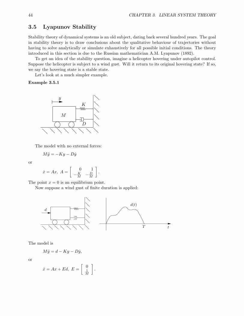
Example 3.5.1
Brief Article
The Author
December 18, 2007
M
y
K
D
1
The model with no external forces:
My = −Ky −Dy
or
x = Ax, A =[
0 1−KM − D
M
].
The point x = 0 is an equilibrium point.Now suppose a wind gust of finite duration is applied:
Brief Article
The Author
December 18, 2007
d
d(t)
T t
1
The model is
My = d−Ky −Dy,
or
x = Ax+ Ed, E =[
01M
].

3.5. LYAPUNOV STABILITY 45
If x(0) = 0, then at time t = T
x(T ) =
T∫0
eA(T−τ)Ed(τ)dτ 6= 0 in general.
For t > T , the model is x = Ax. Thus the effect of a finite-duration disturbance is to alter theinitial state. In this way, the stability question concerns the qualitative behaviour of x = Ax for anarbitrary initial state; the initial time may be shifted to t = 0. 2
We’ll formulate the main concepts for the nonlinear model x = f(x), x(0) = x0, and thenspecialize to the linear one x = Ax, x(0) = x0, for specific results.
Assume the model under study is x = f(x) and assume x = 0 is an equilibrium point, i.e.,f(0) = 0. The stability questions are
1. If x(0) is near the origin, does x(t) remain near the origin? This is stability.
2. Does x(t)→ 0 as t→∞ for every x(0) ? This is asymptotic stability.
To give precise definitions to these concepts, let ‖x‖ denote the Euclidean norm of a vector x,i.e., ‖x‖ = (xTx)1/2 = (Σix
2i )
1/2. Then we say the origin is a stable equilibrium point if
(∀ε > 0)(∃δ > 0)(∀x(0))‖x(0)‖ < δ ⇒ (∀t ≥ 0)‖x(t)‖ < ε.
In words, for every ε > 0 there exists δ > 0 such that if the state starts in the δ-ball, it will remainin the ε-ball:
Brief Article
The Author
December 18, 2007
!
x(t)
"Rn
1
The picture with t explicit is

46 CHAPTER 3. LINEAR SYSTEM THEORY
Brief Article
The Author
December 18, 2007
!x(t)!
!
0t
"
1
Another way of expressing the concept is: the trajectory will remain arbitrarily (i.e., ∀ε) close tothe origin provided it starts sufficiently (i.e., ∃δ) close to the origin.
The origin is an asymptotically stable equilibrium point if
(i) it is stable, and
(ii) (∃ε > 0)(∀x(0))‖x(0)‖ < ε⇒ limt→∞
x(t) = 0.
Clearly the second requirement is that x(t) converges to the origin provided x(0) is sufficiently nearthe origin.
If we’re given the right-hand side function f , it’s in general very hard to determine if theequilibrium point is stable, or asymptotically stable. Because in this course we don’t have time todo the general theory, we’ll look at the results only for the linear system x = Ax,A ∈ Rn×n. Ofcourse, 0 is automatically an equilibrium point. As we saw before, the trajectory is specified byx(t) = eAtx(0). So stability depends on the function t 7−→ eAt : [0,∞)→ Rn×n.
Proposition 3.5.1 For the linear system x = Ax, 0 is stable iff eAt is a bounded function; 0 isasymptotically stable iff eAt → 0 as t→∞.
The condition on A for eAt to be bounded is a little complicated (needs the Jordan form). Thecondition on A for eAt → 0 is pretty easy:
Proposition 3.5.2 eAt → 0 as t→∞ iff every eigenvalue of A has negative real part.
Example 3.5.2
1. x = −x: origin is asymptotically stable
2. x = 0: origin is stable
3. x = x: origin unstable
4.
Brief Article
The Author
December 18, 2007
origin asymp. stable
1

3.5. LYAPUNOV STABILITY 47
5.
Brief Article
The Author
December 18, 2007
origin stable
1
6.
Brief Article
The Author
December 18, 2007
origin asymp. stable
1
7.
Brief Article
The Author
December 18, 2007
origin stable
1
8. maglev
Brief Article
The Author
December 18, 2007
origin unstableorigin unstable
1
2
Proposition 3.5.2 is easy to prove when A has n linearly independent eigenvectors:

48 CHAPTER 3. LINEAR SYSTEM THEORY
eAt = V eDtV −1
eAt → 0⇐⇒ eDt → 0
⇐⇒ eλit → 0 ∀i⇐⇒ Re λi < 0 ∀i.
3.6 BIBO Stability
There’s another stability concept, that concerns the response of a system to inputs instead of initialconditions. We’ll study this concept for a restricted class of systems.
Consider an LTI system with a single input, a single output, and a strictly proper rationaltransfer function. The model is therefore y = g ∗ u in the time domain, or Y (s) = G(s)U(s) inthe s-domain. We ask the question: Does a bounded input (BI) always produce a bounded output(BO)? Note that u(t) bounded means
(∃B)(∀t ≥ 0)|u(t)| ≤ B.
The least upper bound B is actually a norm, denoted ‖u‖∞.
Example 3.6.1
1. u(t) = 1+(t), ‖u‖∞ = 1
2. u(t) = sin(t), ‖u‖∞ = 1
3. u(t) = (1− e−t)1+(t), ‖u‖∞ = 1
4. u(t) = t1+(t), ‖u‖∞ =∞, or undefined.
Note that in the second case, ‖u‖∞ = |u(t)| for some finite t; that is, ‖u‖∞ = maxt≥0|u(t)|. Whereas
in the third case, ‖u‖∞ > |u(t)| for every finite t. 2
We define the system to be BIBO stable if every bounded u produces a bounded y.
Theorem 3.6.1 Assume G(s) is strictly proper, rational. Then the following three statements areequivalent:
1. The system is BIBO stable.
2. The impulse-response function g(t) is absolutely integrable, i.e.,
∞∫0
|g(t)|dt <∞.
3. Every pole of the transfer function G(s) has negative real part.
Example 3.6.2 RC filter

3.6. BIBO STABILITY 49
Brief Article
The Author
December 18, 2007
!
+
u
!
+
y
R
C
1
G(s) =1
RCs+ 1
g(t) =1
RCe−t/RC1+(t)
According to the theorem, every bounded u produces a bounded y. What’s the relationshipbetween ‖u‖∞ and ‖y‖∞? Let’s see:
|y(t)| =
∣∣∣∣∣∣t∫
0
g(t− τ)u(τ)dτ
∣∣∣∣∣∣≤
t∫0
|g(t− τ)||u(τ)|dτ
≤ ‖u‖∞
t∫0
|g(t− τ)|dτ
≤ ‖u‖∞
∞∫0
|g(t)|dt
= ‖u‖∞
∞∫0
1RC
e−t/RCdt
= ‖u‖∞.
Thus ‖y‖∞ ≤ ‖u‖∞ for every bounded u. 2
Example 3.6.3 integrator
G(s) =1s, g(t) = 1+(t)
According to the theorem, the system is not BIBO stable. Thus there exists some bounded inputthat produces an unbounded output. For example
u(t) = 1+(t) = bounded⇒ y(t) = t1+(t) = unbounded.

50 CHAPTER 3. LINEAR SYSTEM THEORY
Notice that it is not true that every bounded input produces an unbounded output, only that somebounded input does. Example
u(t) = (sin t)1+(t)⇒ y(t) bounded.
2
The theorem can be extended to the case where G(s) is only proper (and not strictly proper).Then write
G(s) = c+G1(s), G1(s) strictly proper.
Then the impulse response has the form
g(t) = cδ(t) + g1(t).
The theorem remains true with the second statement changed to say that g1(t) is absolutely inte-grable.
Finally, let’s connect Lyapunov stability and BIBO stability. Consider a single-input, single-output system modeled by
x = Ax+Bu, y = Cx+Du
or
Y (s) = G(s)U(s)
G(s) = C(sI −A)−1B +D
=1
det(sI −A)C adj (sI −A)B +D.
From this last expression it is clear that the poles of G(s) are contained in the set of eigenvalues ofA. Thus
Lyapunov asymptotic stability⇒ BIBO stability.
Usually, the poles of G(s) are identical to the eigenvalues of A, that is, the two polynomials
det(sI −A), C adj (sI −A)B +D det(sI −A)
have no common factors. In this case, the two stability concepts are equivalent. (Don’t forget:We’re discussing only LTI systems.)
Example 3.6.4 MaglevConsider the problem of magnetically levitating a steel ball:

3.6. BIBO STABILITY 51
Brief Article
The Author
December 18, 2007
M
R
+ u
i
dy
L
!
1
u = voltage applied to electromagneti = currenty = position of balld = possible disturbance force
The equations are
Ldi
dt+Ri = u, M
d2y
dt2= Mg + d− c i
2
y2
where c is a constant (force of magnet on ball is proportional to i2/y2). The nonlinear state equationsare
x = f(x, u, d)
x =
yyi
, f =
x2
g +d
M− c
M
x23
x21
−RLx3 +
1Lu
.Let’s linearize about y0 = 1, d0 = 0:
x20 = 0, x10 = 1, x30 =
√Mg
c, u0 = R
√Mg
c.
The linearized system is
∆x = A∆x+B∆u+ E∆d∆y = C∆x
A =
0 1 0
2g 0 −2√
g
Mc
0 0 −RL
, B =
001L
, E =
01M0
C =
[1 0 0
].

52 CHAPTER 3. LINEAR SYSTEM THEORY
To simplify notation, let’s suppose R = L = M = 1, c = g. Then
A =
0 1 02g 0 −20 0 −1
, B =
001
, E =
010
C =
[1 0 0
].
Thus
∆Y (s) = C(sI −A)−1B∆U(s) + C(sI−A)−1E∆D(s)
=−2
(s+ 1)(s2 − 2g)∆U(s) +
1s2 − 2g
∆D(s).
The block diagram is
!U
!D
!Y!2s + 1
1s2 ! 2g
Note that the systems from ∆U to ∆Y and ∆D to ∆Y are BIBO unstable, each having a poleat s =
√2g. To stabilize, we could contemplate closing the loop:
!U
!D
!Y!2s + 1
1s2 ! 2g
?
If we can design a controller (unknown box) so that the system from ∆D to ∆Y is BIBO stable(all poles with Re s < 0 ), then we will have achieved a type of stability. We’ll study this further inthe next chapter. 2
3.7 Frequency Response
Consider a single-input, single-output LTI system. It will then be modeled by
y = g ∗ u or Y (s) = G(s)U(s).
Let us assume G(s) is rational, proper, and has all its poles in Re s < 0. Then the system isBIBO stable.
The first fact we want to see is this: Complex exponentials are eigenfunctions.

3.7. FREQUENCY RESPONSE 53
Proof
u(t) = ejωt, y(t) =
∞∫−∞
g(t− τ)u(τ)dτ
⇒ y(t) =
∞∫−∞
g(t− τ)ejωτdτ
=
∞∫−∞
g(τ)ejωte−jωτdτ
= G(jω)ejωt
2
Thus, if the input is the complex sinusoid ejωt, then the output is the sinusoid
G(jω)ejωt = |G(jω)|ej(ωt+∠G(jw))
which has frequency = ω = frequency of input, magnitude = |G(jω)| = magnitude of the transferfunction at s = jω, and phase = ∠G(jω) = phase of the transfer function at s = jω.
Notice that the convolution equation for this result is
y(t) =
∞∫−∞
g(t− τ)u(τ)dτ,
that is, the sinusoidal input was applied starting at t = −∞. If the time of application of thesinusoid is t = 0, there is a transient component in y(t) too.
Next, we want to look at the special frequency response when ω = 0. For this we need thefinal-value theorem.
Example 3.7.1 Let y(t), Y (s) be Laplace transform pairs with Y (s) =s+ 2
s(s2 + s+ 4).
This can be factored as
Y (s) =A
s+
Bs+ C
s2 + s+ 4.
Note that A equals the residue of Y (s) at the pole s = 0:
A = Res (Y, 0) = lims→0
s Y(s) =12.
The inverse LT then has the form
Y (t) = A1+(t) + y1(t),
where y1(t)→ 0 as t→∞. Thus
limt→∞
y(t) = A = Res (Y, 0).
2
The general result is the final-value theorem:

54 CHAPTER 3. LINEAR SYSTEM THEORY
Theorem 3.7.1 Suppose Y (s) is rational.
1. If Y (s) has no poles in <s ≥ 0, then y(t) converges to 0 as t→∞.
2. If Y (s) has no poles in <s ≥ 0 except a simple pole at s = 0, then y(t) converges as t → ∞and limt→∞ y(t) equals the residue of Y (s) at the pole s = 0.
3. If Y (s) has a repeated pole at s = 0, then y(t) doesn’t converge as t→∞.
4. If Y (s) has a pole at <s ≥ 0, s 6= 0, then y(t) doesn’t converge as t→∞.
Some examples: Y (s) =1
s+ 1: final value equals 0; Y (s) =
2s(s+ 1)
: final value equals 2;
Y (s) =1
s2 + 1: no final value. Remember that you have to know that y(t) has a final value, by
examining the poles of Y (s), before you calculate the residue of Y (s) at the pole s = 0 and claimthat that residue equals the final value.
Return now to the setup
Y (s) = G(s)U(s), G(s) proper, no poles in Re s ≥ 0.
Let the input be the unit step, u(t) = 1+(t), i.e., U(s) =1s
. Then Y (s) = G(s)1s
. The final-value
theorem applies to this Y (s), and we get limt→∞
y(t) = G(0). For this reason, G(0) is called the DC
gain of the system.
Example 3.7.2 Using MATLAB, plot the step responses of
G1(s) =20
s2 + 0.9s+ 50, G2(s) =
−20s+ 20s2 + 0.9s+ 50
.
They have the same DC gains and the same poles, but notice the big difference in transient response.
2
3.8 Problems
1. Find the transition matrix for
A =
1 1 0−1 1 0
0 0 0
by two different methods (you may use Scilab or MATLAB).
2. Consider the system x = Ax, x(0) = x0. Let T be a positive sampling period. The sampledstate sequence is
x(0), x(T ), x(2T ), . . . .
Derive an iterative equation for obtaining the state at time (k + 1)T from the state at timekT .

3.8. PROBLEMS 55
3. Consider a system modeled by
x = Ax+Bu, y = Cx+Du,
where dimu = dim y = 1, dimx = 2.
(a) Given the initial-state-responses
x(0) =[
10.5
]=⇒ y(t) = e−t − 0.5e−2t
x(0) =[−11
]=⇒ y(t) = −0.5e−t − e−2t,
find the initial-state-response for x(0) =[
20.5
].
(b) Now suppose
x(0) =[
11
], u a unit step =⇒ y(t) = 0.5− 0.5e−t + e−2t
x(0) =[
22
], u a unit step =⇒ y(t) = 0.5− e−t + 1.5e−2t.
Find y(t) when u is a unit step and x(0) = 0.
4. This problem requires formal logic.
(a) Write the definition that the function f : R→ R is not continuous at t = 0.
(b) Prove that the unit step 1+(t) satisfies the previous definition.
(c) Write the definition that the equilibrium 0 of the system x = f(x) is not stable.
(d) Prove that the equilibrium point 0 of the system x = x satisfies the previous definition.
5. Consider x = Ax with
A =
0 −2 −10 −1 01 0 0
.Is the origin asymptotically stable? Find an x(0) 6= 0 such that x(t)→ 0 as t→∞.
6. Consider x = Ax.
(a) Prove that the origin is stable if
A =[
0 1−1 0
].
(b) Prove that the origin is unstable if
A =[
0 10 0
].

56 CHAPTER 3. LINEAR SYSTEM THEORY
7. Consider the cart-spring system. Its equation of motion is
My +Ky = 0,
where M > 0, K > 0. Take the natural state and prove that the origin is stable. (For anarbitrary ε, you must give an explicit δ.)
8. Consider the convolution equation y = g ? u, where g(t) is absolutely integrable, that is, thesystem is BIBO stable.. The inequality
‖y‖∞ ≤ ‖u‖∞∫ ∞
0|g(t)|dt
is derived in the course notes. Show that this is the best bound; that is, construct a nonzeroinput u(t) for which the inequality is an equality.
9. Consider the maglev example, Example 3.6.4. Is there a constant gain to put in the unknownbox so that the system from ∆D to ∆Y is BIBO stable?
10. Give an example of a continuously differentiable, bounded, real-valued function defined on theopen interval (0, 1) whose derivative is not bounded on that interval. What can you concludeabout BIBO stability of the differentiator? Discuss stability of the differentiator in the senseof Lyapunov.
11. The transfer function of an LC circuit is G(s) = 1/(LCs2 + 1).
(a) Is the output bounded if the input is the unit step?
(b) Prove that the circuit is not a BIBO stable system.
12. A rubber ball is tossed straight into the air, rises, then falls and bounces from the floor, rises,falls, and bounces again, and so on. Let c denote the coefficient of restitution, that is, theratio of the velocity just after a bounce to the velocity just before the bounce. Thus 0 < c < 1.Neglecting air resistance, show that there are an infinite number of bounces in a finite timeinterval.
Hint: Assume the ball is a point mass. Let x(t) denote the height of the ball above the floorat time t. Then x(0) = 0, x(0) > 0. Model the system before the first bounce and calculatethe time of the first bounce. Then specify the values of x, x just after the first bounce. Andso on.
13. The linear system x = Ax can have more than one equilibrium point.
(a) Characterize the set of equilibrium points. Give an example A for which there’s morethan one.
(b) Prove that if one equilibrium point is stable, they all are.

Chapter 4
Feedback Control Theory
Feedback is a miraculous invention. In this chapter we’ll see why.
4.1 Closing the Loop
As usual, we start with an example.
Example 4.1.1 linearized cart-pendulum
Brief Article
The Author
January 29, 2008
M1
u
M2x1
L
x2
1
The figure defines x1, x2. Now define x3 = x1, x4 = x2. Take M1 = 1 Kgm, M2 = 2 Kgm, L = 1m, g = 9.8 m/s2. Then the state model is
x = Ax+Bu, A =
0 0 1 00 0 0 10 −19.6 0 00 29.4 0 0
, B =
001−1
.Let’s suppose we measure the cart position only: y = x1. Then
C =[
1 0 0 0].
57

58 CHAPTER 4. FEEDBACK CONTROL THEORY
The transfer function from u to y is
P (s) =s2 − 9.8
s2(s2 − 29.4).
The poles and zeros of P (s) are
Brief Article
The Author
January 29, 2008
X X
-5.4 -3.13 3.13 5.4
XX
1
Having three poles in Re s ≥ 0, the plant is quite unstable. The right half-plane zero doesn’tcontribute to the degree of instability, but, as we shall see, it does make the plant quite difficult tocontrol. The block diagram of the plant by itself is
Brief Article
The Author
January 29, 2008
y
force oncart, N
position of cart, m
uP (s)
1
Let us try to stabilize the plant by feedback:
Brief Article
The Author
January 29, 2008
C(s) P (s)yr u
!
1
Here r is the reference position of the cart and C(s) is the transfer function of the controller to bedesigned. One controller that does in fact stabilize is
C(s) =10395s3 + 54126s2 − 13375s− 6687s4 + 32s3 + 477s2 − 5870s− 22170
.
You’re invited to simulate the closed-loop system; for example, let r be the input
Brief Article
The Author
January 29, 2008
r
0.1
5 t
1
4.1. CLOSING THE LOOP 59
which corresponds to a command that the cart move right 0.1 m for 5 seconds, then return to itsoriginal position. Plot x1 and x2, the cart and pendulum positions. 2
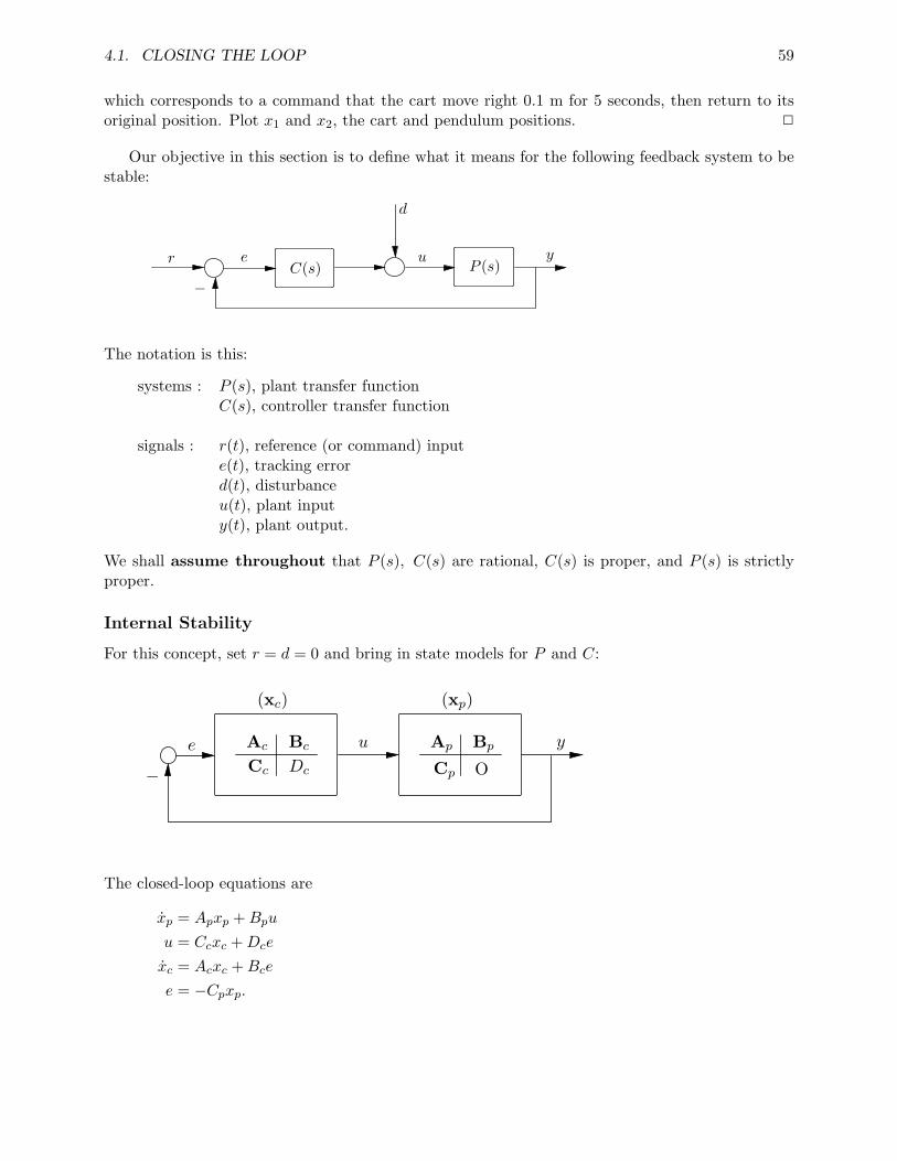
Our objective in this section is to define what it means for the following feedback system to bestable:
Brief Article
The Author
January 29, 2008
P (s)y
C(s)
d
ur e
!
1
The notation is this:
systems : P (s), plant transfer functionC(s), controller transfer function
signals : r(t), reference (or command) inpute(t), tracking errord(t), disturbanceu(t), plant inputy(t), plant output.
We shall assume throughout that P (s), C(s) are rational, C(s) is proper, and P (s) is strictlyproper.
Internal Stability
For this concept, set r = d = 0 and bring in state models for P and C:
Brief Article
The Author
January 29, 2008
DcCc
Ac Bc
(xc) (xp)
Ap Bp
!
e yu
OCp
1
The closed-loop equations are
xp = Apxp +Bpu
u = Ccxc +Dce
xc = Acxc +Bce
e = −Cpxp.

60 CHAPTER 4. FEEDBACK CONTROL THEORY
Defining the closed-loop state xcl = (xp, xx), we get simply
xcl = Aclxcl, Acl =[Ap −BpDcCp BpCc−BcCp Ac
].
Internal Stability is defined to mean that the origin is an asymptotically stable equilibriumpoint, that is, that all the eigenvalues of Acl have Re λ < 0. Thus the concept means this: With noinputs applied (i.e., r = d = 0), the internal states xp(t), xc(t) will converge to zero for every initialstate xp(0), xc(0).
Example 4.1.2
Take C(s) = 2, P (s) = 1/(s− 1). Then
Ap = 1, Bp = 1, Cp = 1; Dc = 2
and
Acl = Ap −BpDcCp = −1.
Thus the unstable plant1
s− 1is internally stabilized by unity feedback with the pure-gain controller
2. 2
Example 4.1.3
Let’s see that 1/(s− 1) cannot be internally stabilized by cancelling the unstable pole:
Brief Article
The Author
February 1, 2008
(xc) (xp)
yur s ! 1
s + 1
1
s ! 1
1
The transfer function from r to y equals1
s+ 1. Hence the system from r to y is BIBO stable. But
with r = 0, the state model is
Brief Article
The Author
February 1, 2008
-1 1
(xc) (xp)
1
01
0 1
-2 1
1
Thus
xp = xp − 2xcxc = −xc
xcl = Aclxcl, Acl =[
1 −20 −1
]= unstable.
Clearly xp(t) doesn’t converge to 0 if xp(0) 6= 0. 2

4.1. CLOSING THE LOOP 61
Input-Output Stability
Now we turn to the second way of thinking about stability of the feedback loop. First, let’s solvefor the outputs of the summing junctions:
E = R− PUU = D + CE[
1 P−C 1
] [EU
]=[RD
].
In view of our standing assumptions (P strictly proper, C proper), the determinant of[1 P
−C 1
]is not identically zero (why?). Thus
[EU
]=[
1 P−C 1
]−1 [RD
]=
1
1 + PC
−P1 + PC
C
1 + PC
11 + PC
[ RD
]
Y = PU =PC
1 + PCR+
P
1 + PCD.
We just derived the following closed-loop transfer functions:
R to E :1
1 + PC, R to U :
C
1 + PC, R to Y :
PC
1 + PC
D to E :−P
1 + PC, D to U :
11 + PC
, D to Y :P
1 + PC.
The above method of finding closed-loop transfer functions works in general.
Example 4.1.4
Brief Article
The Author
February 1, 2008
r y
P4
!
x1
P3
x2 P2
P5
P1
!
1

62 CHAPTER 4. FEEDBACK CONTROL THEORY
Let us find the transfer function from r to y. Label the outputs of the summing junctions, as shown.Write the equations at the summing junctions:
X1 = R− P2P5X2
X2 = P1X1 − P2P4X2
Y = P3X1 + P2X2.
Assemble as 1 P2P5 0−P1 1 + P2P4 0−P3 −P2 1
X1
X2
Y
=
R00
.Solve for Y by Cramer’s rule:
Y =
det
1 P2P5 R−P1 1 + P2P4 0−P3 −P2 0
det
1 P2P5 0−P1 1 + P2P4 0−P3 −P2 1
.
Simplify:
Y
R=P1P2 + P3(1 + P2P4)1 + P2P4 + P1P2P5
.
2
Now back to
Brief Article
The Author
February 1, 2008
y
d
ur e
!
C P
1
We say the feedback system is input-output stable provided e, u, and y are bounded signalswhenever r and d are bounded signals; briefly, the system from (r, d) to (e, u, y) is BIBO stable.This is equivalent to saying that the 6 transfer funtions from (r, d) to (e, u, y) are stable, in thesense that all poles are in Re s < 0. It suffices to look at the 4 transfer functions from (r, d) to(e, u), namely,
11 + PC
−P1 + PC
C
1 + PC
11 + PC
.
(Proof: If r and e are bounded, so is y = r − e.)

4.1. CLOSING THE LOOP 63
Example 4.1.5
P (s) =1
s2 − 1, C(s) =
s− 1s+ 1
The 4 transfer functions are
[EU
]=
(s+ 1)2
s2 + 2s+ 2s+ 1
(s− 1)(s2 + 2s+ 2)
(s+ 1)(s− 1)s2 + 2s+ 2
(s+ 1)2
s2 + 2s+ 2
[RD
].
Three of these are stable; the one from D to E is not. Consequently, the feedback system is notinput-output stable. This is in spite of the fact that a bounded r produces a bounded y. Noticethat the problem here is that C cancels an unstable pole of P . As we’ll see, that isn’t allowed.
2
Example 4.1.6
P (s) =1
s− 1, C(s) = k
The feedback system is input-output stable iff k > 1 (check). 2
We now look at two ways to test feedback IO stability. The first is in terms of numerator anddenominator polynomials:
P =Np
Dp, C =
Nc
Dc.
We assume (Np, Dp) are coprime, i.e., have no common factors, and (Nc, Dc) are coprime too.The characteristic polynomial of the feedback system is defined to be NpNc +DpDc.
Example 4.1.7
P (s) =1
s2 − 1, C(s) =
s− 1s+ 1
The characteristic polynomial is
s− 1 + (s2 − 1)(s+ 1) = (s− 1)(s2 + 2s+ 2).
2
Theorem 4.1.1 The feedback system is input-output stable iff the char poly has no roots in Re s ≥0.
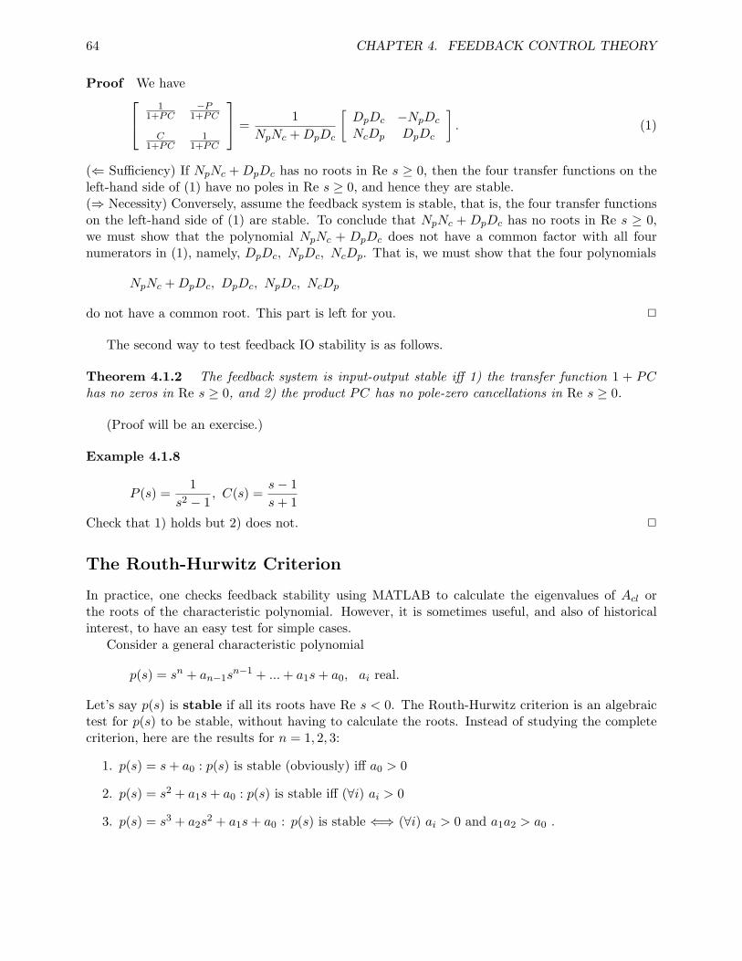
64 CHAPTER 4. FEEDBACK CONTROL THEORY
Proof We have 11+PC
−P1+PC
C1+PC
11+PC
=1
NpNc +DpDc
[DpDc −NpDc
NcDp DpDc
]. (1)
(⇐ Sufficiency) If NpNc + DpDc has no roots in Re s ≥ 0, then the four transfer functions on theleft-hand side of (1) have no poles in Re s ≥ 0, and hence they are stable.(⇒ Necessity) Conversely, assume the feedback system is stable, that is, the four transfer functionson the left-hand side of (1) are stable. To conclude that NpNc + DpDc has no roots in Re s ≥ 0,we must show that the polynomial NpNc + DpDc does not have a common factor with all fournumerators in (1), namely, DpDc, NpDc, NcDp. That is, we must show that the four polynomials
NpNc +DpDc, DpDc, NpDc, NcDp
do not have a common root. This part is left for you. 2
The second way to test feedback IO stability is as follows.
Theorem 4.1.2 The feedback system is input-output stable iff 1) the transfer function 1 + PChas no zeros in Re s ≥ 0, and 2) the product PC has no pole-zero cancellations in Re s ≥ 0.
(Proof will be an exercise.)
Example 4.1.8
P (s) =1
s2 − 1, C(s) =
s− 1s+ 1
Check that 1) holds but 2) does not. 2
The Routh-Hurwitz Criterion
In practice, one checks feedback stability using MATLAB to calculate the eigenvalues of Acl orthe roots of the characteristic polynomial. However, it is sometimes useful, and also of historicalinterest, to have an easy test for simple cases.
Consider a general characteristic polynomial
p(s) = sn + an−1sn−1 + ...+ a1s+ a0, ai real.
Let’s say p(s) is stable if all its roots have Re s < 0. The Routh-Hurwitz criterion is an algebraictest for p(s) to be stable, without having to calculate the roots. Instead of studying the completecriterion, here are the results for n = 1, 2, 3:
1. p(s) = s+ a0 : p(s) is stable (obviously) iff a0 > 0
2. p(s) = s2 + a1s+ a0 : p(s) is stable iff (∀i) ai > 0
3. p(s) = s3 + a2s2 + a1s+ a0 : p(s) is stable ⇐⇒ (∀i) ai > 0 and a1a2 > a0 .

4.2. THE INTERNAL MODEL PRINCIPLE 65
4.2 The Internal Model Principle
A thermostat-controlled temperature regulator controls temperature to a prescribed setpoint. Like-wise, cruise control in a car regulates the speed to a prescribed setpoint. What is the principleunderlying their operation? The answer lies in the final value theorem (FVT).
Example 4.2.1
Brief Article
The Author
February 1, 2008
C(s) P (s)!
e(t)r(t)
1
Take the controller and plant
C(s) =1s, P (s) =
1s+ 1
.
Let r be a constant, r(t) = r0. Then we have
E(s) =1
1 + P (s)C(s)R(s)
=s(s+ 1)s2 + s+ 1
r0
s
=s+ 1
s2 + s+ 1r0
The FVT applies to E(s), and e(t) → 0 as t → ∞. Thus the feedback system provides perfectasymtotic tracking of a step input! How it works: C(s) contains an internal model of R(s) (i.e., anintegrator); closing the loop creates a zero from R(s) to E(s) exactly to cancel the unstable poleof R(s). (This isn’t illegal pole-zero cancellation.) 2
Example 4.2.2
This time take
C(s) =1s, P (s) =
2s+ 1s(s+ 1)
and take r to be a ramp, r(t) = r0t. Then R(s) = r0/s2 and so
E(s) =s+ 1
s3 + s2 + 2s+ 1r0.
Again e(t) → 0; perfect tracking of a ramp. Here C(s) and P (s) together provide the internalmodel, a double integrator. 2
Let’s generalize:

66 CHAPTER 4. FEEDBACK CONTROL THEORY
Theorem 4.2.1 Assume P (s) is strictly proper, C(s) is proper, and the feedback system is stable.If P (s)C(s) contains an internal model of the unstable part of R(s), then perfect asymptotic trackingoccurs, i.e., e(t)→ 0.
Example 4.2.3
R(s) =r0
s2 + 1, P (s) =
1s+ 1
Design C(s) to achieve perfect asymptotic tracking of the sinusoid r(t), as follows. From thetheorem, we should try something of the form
C(s) =1
s2 + 1C1(s),
that is, we embed an internal model in C(s), and allow an additional factor to achieve feedbackstability. You can check that C1(s) = s works. Notice that we have effectively created a notch filterfrom R to E, a notch filter with zeros at s = ±j. 2
Example 4.2.4
An inverted pendulum balanced on your hand.
Brief Article
The Author
February 1, 2008
Mg
M
u
L
!
u + L!
1
The equation is
u+ Lθ = Mgθ.
Thus
s2U + s2Lθ = Mgθ.
So the transfer function from u to θ equals
−s2
Ls2 −Mg.
Step tracking and internal stability are not simultaneously achievable. 2

4.3. PRINCIPLE OF THE ARGUMENT 67
4.3 Principle of the Argument
This section and the following two develop the Nyquist stability criterion.
Consider a closed path D in the s-plane, with no self-intersections and with negative, i.e.,clockwise (CW) orientation.
Brief Article
The Author
February 2, 2008
s-plane
D
1
Let G(s) be a rational function. As s goes once around D from any starting point, the point G(s)traces out a closed curve denoted G, the image of D under G(s).
Example 4.3.1
G(s) = s− 1
Brief Article
The Author
February 2, 2008
G
G-plane
G(s)
D
1
s
s ! 1
s-plane
1
D encircles one zero of G(s); G encircles the origin once CW. 2
Example 4.3.2
G(s) = s− 1
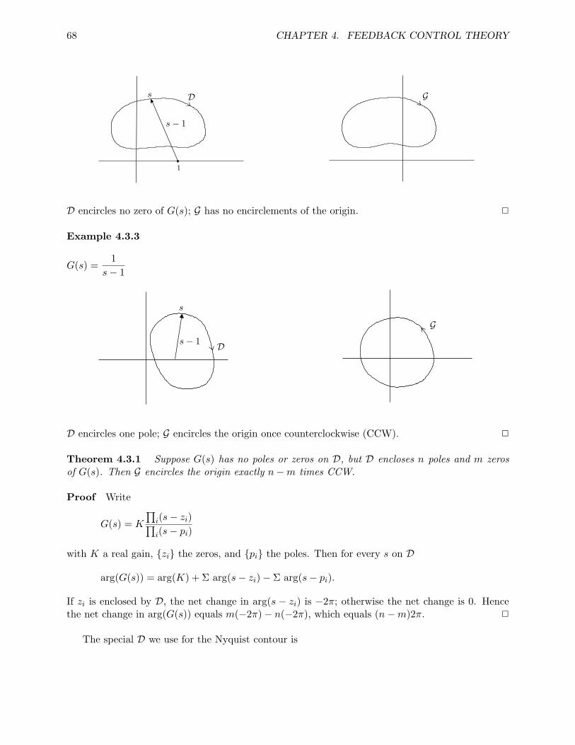
68 CHAPTER 4. FEEDBACK CONTROL THEORY
Brief Article
The Author
February 2, 2008
s
s ! 1
1
GD
1
D encircles no zero of G(s); G has no encirclements of the origin. 2
Example 4.3.3
G(s) =1
s− 1
Brief Article
The Author
February 2, 2008
s ! 1
G
D
s
1
D encircles one pole; G encircles the origin once counterclockwise (CCW). 2
Theorem 4.3.1 Suppose G(s) has no poles or zeros on D, but D encloses n poles and m zerosof G(s). Then G encircles the origin exactly n−m times CCW.
Proof Write
G(s) = K
∏i(s− zi)∏i(s− pi)
with K a real gain, {zi} the zeros, and {pi} the poles. Then for every s on D
arg(G(s)) = arg(K) + Σ arg(s− zi)− Σ arg(s− pi).
If zi is enclosed by D, the net change in arg(s − zi) is −2π; otherwise the net change is 0. Hencethe net change in arg(G(s)) equals m(−2π)− n(−2π), which equals (n−m)2π. 2
The special D we use for the Nyquist contour is

4.4. NYQUIST STABILITY CRITERION (1932) 69
Brief Article
The Author
February 2, 2008
radius ! "
1
Then G is called the Nyquist plot of G(s). If G(s) has no poles or zeros on D, then the Nyquistplot encircles the origin exactly n−m times CCW, where n equals the number of poles of G(s) inRe s > 0 and m equals the number of zeros of G(s) in Re s > 0. From this follows
Theorem 4.3.2 Suppose G(s) has no poles on D. Then G(s) has no zeros in Re s ≥ 0 ⇔ Gdoesn’t pass through the origin and encircles it exactly n times CCW, where n equals the number ofpoles in Re s > 0.
Note that G(s) has no poles on D iff G(s) is proper and G(s) has no poles on the imaginary axis,and G(s) has no zeros on D iff G(s) is not strictly proper and G(s) has no zeros on the imaginaryaxis.
In our application, if G(s) actually does have poles on the imaginary axis, we have to indentaround them. You can indent either to the left or to the right; we shall always indent to the right:
Brief Article
The Author
February 2, 2008
x
x
x
x
D
poles
1
4.4 Nyquist Stability Criterion (1932)
This beautiful stability criterion is due to a mathematician, Harry Nyquist, who worked at AT&Tand was asked by some engineers to study the problem of stability in feedback amplifiers.
The setup is
Brief Article
The Author
February 2, 2008
P (s)!
KC(s)
1
where K is a real gain. We’re after a graphical test for stability involving the Nyquist plot ofP (s)C(s).

70 CHAPTER 4. FEEDBACK CONTROL THEORY
The assumptions are that P (s), C(s) are proper, with P (s)C(s) strictly proper, the productP (s)C(s) has no pole-zero cancellations in Re s ≥ 0, and K 6= 0.
Theorem 4.4.1 Let n denote the number of poles of P (s)C(s) in Re s > 0. Construct theNyquist plot of P (s)C(s), indenting to the right around poles on the imaginary axis. Then thefeedback system is stable iff the Nyquist plot doesn’t pass through − 1
K and encircles it exactly ntimes CCW.
Proof Define G(s) = 1 + KP (s)C(s). By Theorem 4.3.2, the feedback system is stable iff G(s)has no zeros in Re s ≥ 0. Note that G(s) and P (s)C(s) have the same poles in Re s ≥ 0, soG(s) has precisely n there. Since D indents around poles of G(s) on the imaginary axis and sinceG(s) is proper, G(s) has no poles on D. Thus by Theorem 4.1.2, the feedback system is stable⇔ the Nyquist plot of G(s) doesn’t pass through 0 and encircles it exactly n times CCW. Since
P (s)C(s) =1KG(s)− 1
K, this latter condition is equivalent to: the Nyquist plot of P (s)C(s) doesn’t
pass through − 1K and encircles it exactly n times CCW. 2
4.5 Examples
Example 4.5.1 PC(s) =1
(s+ 1)2
Re PC(jω) =1− ω2
(1− ω2)2 + (2ω)2, Im PC(jω) =
−2ω(1− ω2)2 + (2ω)2
Brief Article
The Author
February 2, 2008
1
B
A
C
D
B, C A
Nyquist plot of PC
1
n = 0. Therefore the feedback system is stable iff −1/K < 0 or −1/K > 1; that is, K > 0 or−1 < K < 0; that is, K > −1,K 6= 0. The condition K 6= 0 is ruled out by assumption. But wecan check now that the feedback system actually is stable for K = 0. So finally the condition isK > −1. 2
Example 4.5.2 PC(s) =s+ 1s(s− 1)
Re PC(jω) = − 2ω2 + 1
, Im PC(jω) =1− ω2
ω(ω2 + 1)

4.6. STABILITY AND BODE PLOTS 71
Brief Article
The Author
February 2, 2008
xx
D
DA
B
C D
-1
-2
A
B, C
1
n = 1. Feedback stability iff −1 < −1/K < 0; equivalently, K > 1. 2
Example 4.5.3 PC(s) =1
(s+ 1)(s2 + 1)
Re PC(jω) =1
1− ω4, Im PC(jω) =
−ω1− ω4
Brief Article
The Author
February 2, 2008
x
x
x
xC
D
A
G
E
D
C
+1 G
A
BF
ED
1
-1
B
F
1
n = 0. Feedback stability iff −1/K > 1; equivalently, −1 < K < 0. 2
Shortcuts:
1. Principle of conformal mapping.
2. If an indentation in D bypasses a pole of multiplicity k, the Nyquist plot will go through kπradians.
4.6 Stability and Bode Plots
Control design is typically done in the frequency domain using Bode plots. For this reason it’suseful to translate the Nyquist criterion into a condition on Bode plots.
First, let’s review the drawing of Bode plots. (You’re likely to be unfamiliar with these whenthe plant has right half-plane poles or zeros.) We consider only rational G(s) with real coefficients.Then G(s) has a numerator and denominator, each of which can be factored into terms of thefollowing forms:
1. gain: K

72 CHAPTER 4. FEEDBACK CONTROL THEORY
2. pole or zero at s = 0 : sn
3. real nonzero pole or zero : τs± 1
4. complex conjugate pole or zero :1ω2n
(s2 ± 2ζωns+ ω2n), ωn > 0, 0 ≤ ζ < 1
For example
G(s) =40s2(s− 2)
(s− 5)(s2 + 4s+ 100)
=40× 25× 100
s2(12s− 1)
(15s− 1)[ 1
100(s2 + 4s+ 100)].
As an intermediate step, we introduce the polar plot : ImG(jω) vs Re G(jω) as ω : 0→∞.We now look at polar and Bode plots for each of the four terms.
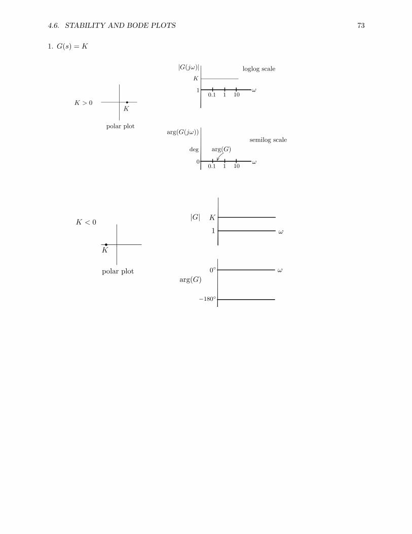
4.6. STABILITY AND BODE PLOTS 73
1. G(s) = K
Brief Article
The Author
February 2, 2008
polar plot
K > 0K
|G(j!)|
10
K
10.1
loglog scale
100
0.1
semilog scale
deg
arg(G(j!))
arg(G)
1
1
!
!
1
Brief Article
The Author
February 2, 2008
polar plot
K < 0
K
K
1
|G|
!
!
arg(G)0!
!180!
1

74 CHAPTER 4. FEEDBACK CONTROL THEORY
2. G(s) = sn, n ≥ 1
Brief Article
The Author
February 2, 2008
0.1
1 10
1
0.1
0.1
1 10
1
0.1
|G|10 n
!
n = 2
n = 3arg(G)
180
270
90
0
n = 1
n = 4, 8, ...
n = 3, 7, ...
n = 2, 6, ...
n = 1, 5, ...
polar plot
1

4.6. STABILITY AND BODE PLOTS 75
3. G(s) = τs+ 1, τ > 0
Brief Article
The Author
February 2, 2008
11
1 decade
= |1 + j| =!
2 = 3dB
1
|G|
exact
approx
+1
polar plot
maxerror
G(j!) = 1 + j"!
LHP zero
1
!= corner freq.
approx
exact
0.1
!
10
!
arg(G)
90!
0!
1
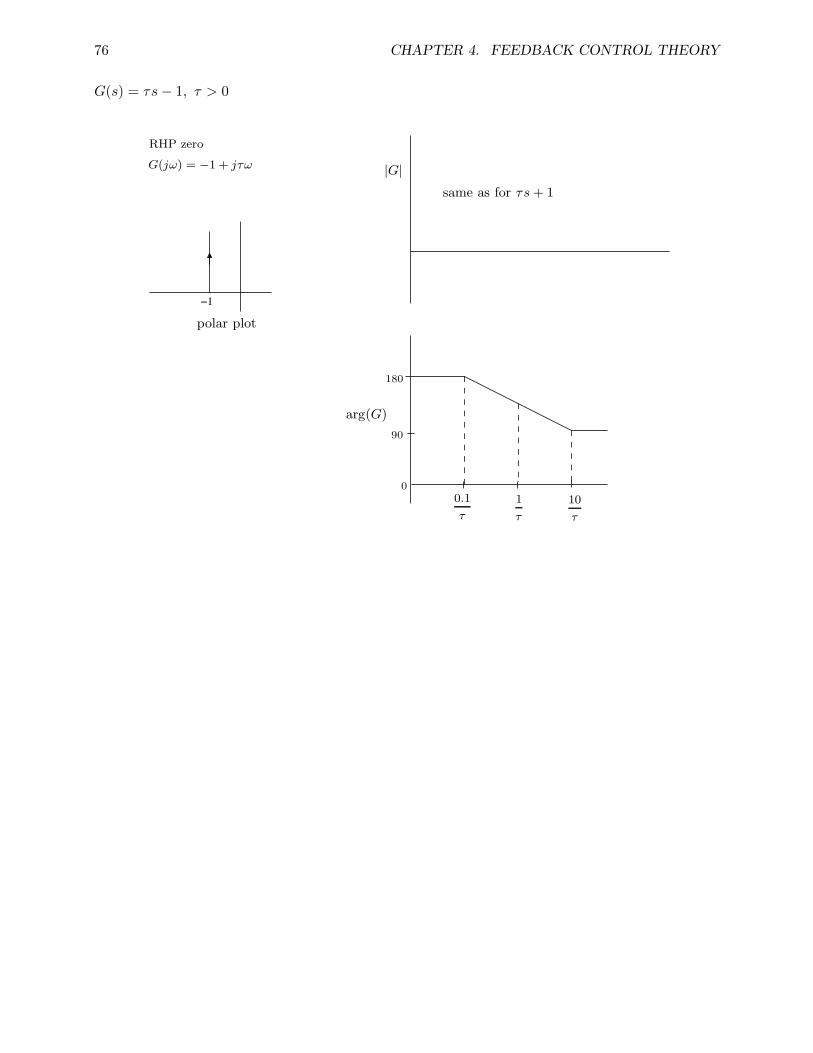
76 CHAPTER 4. FEEDBACK CONTROL THEORY
G(s) = τs− 1, τ > 0
Brief Article
The Author
February 2, 2008
!1!1
G(j!) = !1 + j"!
RHP zero
|G|
same as for !s + 1
180
90
0
0.1
"
arg(G)
1
"
10
"
polar plot
1
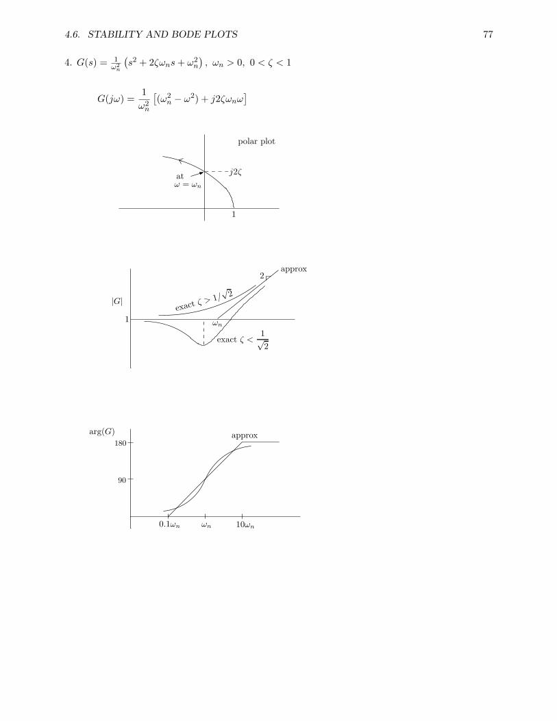
4.6. STABILITY AND BODE PLOTS 77
4. G(s) = 1ω2
n
(s2 + 2ζωns+ ω2
n
), ωn > 0, 0 < ζ < 1
G(jω) =1ω2n
[(ω2n − ω2) + j2ζωnω
]
0.1!n !n
90
approx
10!n
180
arg(G)
polar plot
j2"
1
at! = !n
1
2
exact " <1!2
approx
exact " > 1/!
2
!n
|G|
2

78 CHAPTER 4. FEEDBACK CONTROL THEORY
G(s) =1ω2n
(s2 + ω2n), ωn > 0 (i.e., ζ = 0)
Brief Article
The Author
February 2, 2008
1
polar plot
1
polar plot
1
|G| approx
exact!n
180
0!n
arg(G)
1
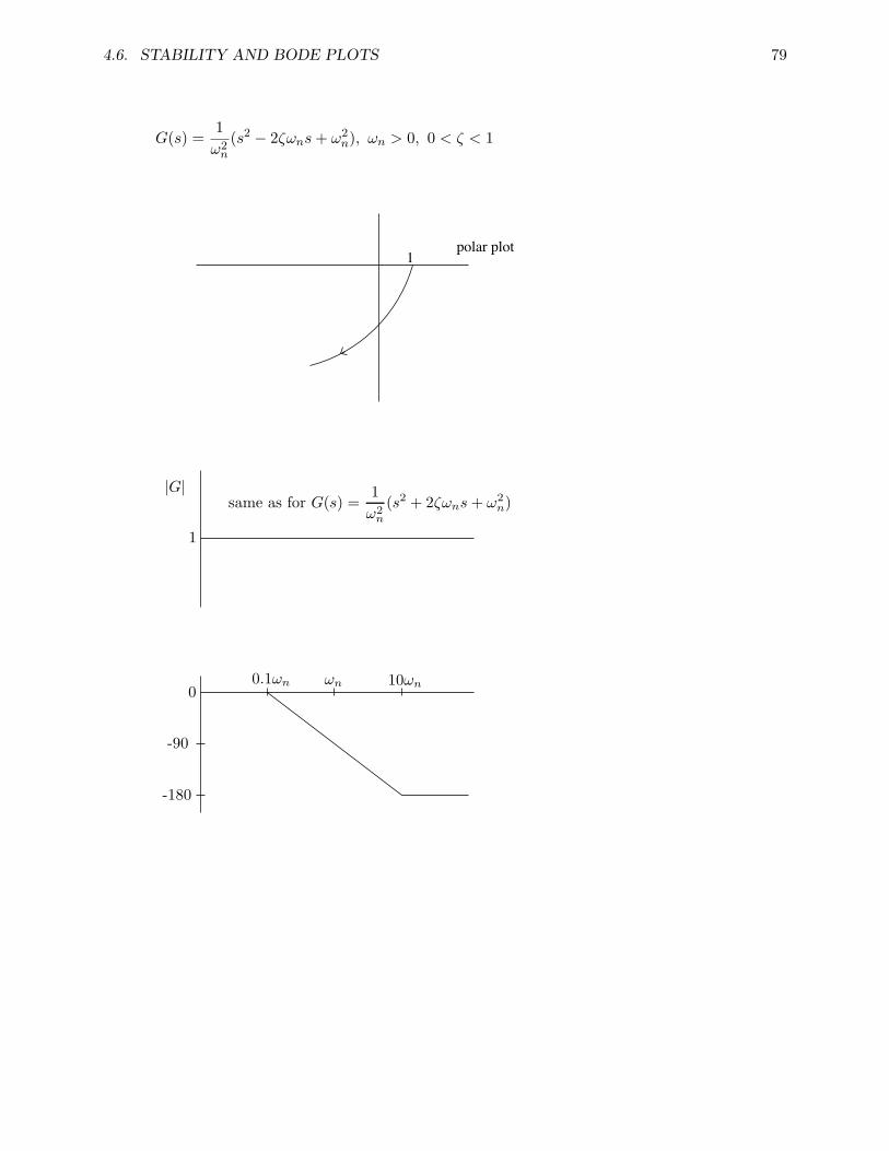
4.6. STABILITY AND BODE PLOTS 79
G(s) =1ω2n
(s2 − 2ζωns+ ω2n), ωn > 0, 0 < ζ < 1
Brief Article
The Author
February 2, 2008
1polar plot
1polar plot
|G|
1
same as for G(s) =1
!2n
(s2 + 2"!ns + !2
n)
0
-90
-180
0.1!n !n 10!n
1
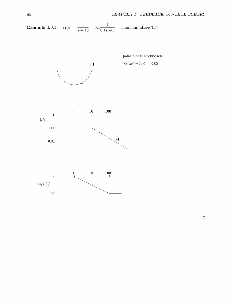
80 CHAPTER 4. FEEDBACK CONTROL THEORY
Example 4.6.1 G1(s) =1
s+ 10= 0.1
10.1s+ 1
minimum phase TF
0.1
polar plot is a semicircle:
|G(j!) ! 0.05| = 0.05
-1
10 100
10 1001
0.1
1|G1|
-90
0
arg(G1)
0.01
1
2
2

4.6. STABILITY AND BODE PLOTS 81
Example 4.6.2 G2(s) =1− s1 + s
allpass TF
polar plot
1
|G2|
0
arg(G2)
-180
0.1 1 10
2
2

82 CHAPTER 4. FEEDBACK CONTROL THEORY
Example 4.6.3
G3 = G1G2 nonminimum phase TF
G3(s) =1
s+ 101− s1 + s
|G3(jω)| = |G1(jω)|arg(G3) = arg(G1) + arg(G2) ≤ arg(G1)
Brief Article
The Author
February 2, 2008
!90
!180
!270
0.1 1 10 100
!90
!180
!270
0.1 1 10 100
arg(G2)
arg(G1)
arg(G3)
phase lag at ! = 10
1
Of all TFs having the magnitude plot |G1|, G1 has the minimum phase lag at every ω. 2

4.6. STABILITY AND BODE PLOTS 83
Using the principles developed so far, you should be able to sketch the approximation of theBode plot of
G(s) =40s2(s− 2)
(s− 5)(s2 + 4s+ 100)
= 0.16s2(1
2s− 1)(1
5s− 1)[ 1100(s2 + 4s+ 100)]
.
Now let’s see how to deduce feedback stability from Bode plots.
Example 4.6.4
Brief Article
The Author
February 2, 2008
C(s) P (s)!
1
C(s) = 2, P (s) =1
(s+ 1)2
The Nyquist plot is
Brief Article
The Author
February 2, 2008
!1!1 2
critical pt
this angle iscalled thephase margin
1
There are no encirclements of the critical point, so the feedback system is stable. The Bode plot ofPC is
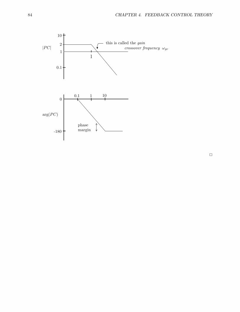
84 CHAPTER 4. FEEDBACK CONTROL THEORY
Brief Article
The Author
February 2, 2008
0.1 10
1
crossover frequency
this is called the gain
phasemargin
0
arg(PC)
0.1
-180
1
|PC|1
2
10
!gc
1
2

4.6. STABILITY AND BODE PLOTS 85
Example 4.6.5
C(s) = 2, P (s) =1
(s+ 1)2(0.1s+ 1)
Brief Article
The Author
February 2, 2008
(half shown)2crit.pt.
-1
Nyquist :!
1
12.1
1
Stable for C(s) = 2K and − 1K
< − 112.1
. Thus max K = 12.1 = 21.67 dB. See how this appearson the Bode plot. 2

86 CHAPTER 4. FEEDBACK CONTROL THEORY
4.6. STABILITY AND BODE PLOTS 87
Frequency (rad/sec)
Phase (
deg); M
agnitude (
dB
)
Bode Diagrams
!100
!80
!60
!40
!20
0
20
Gm=21.656 dB (at 4.5826 rad/sec), Pm=84.6 deg. (at 0.99507 rad/sec)
10!1
100
101
102
!300
!250
!200
!150
!100
!50
0
Figure 4.1: Example 4.6.5

4.6. STABILITY AND BODE PLOTS 87
Example 4.6.6 C(s) = 2, P (s) =s+ 1s(s− 1)
The Nyquist plot of PC has the form
Brief Article
The Author
February 2, 2008
-2
1
The critical point is -1 and we need 1 CCW encirclement, so the feedback system is stable. Thephase margin on the Nyquist plot:
Brief Article
The Author
February 2, 2008
-1
36.9!
1
If C(s) = 2K, K can be reduced until − 1K
= −2, i.e., min K =12
= 6 dB. The Bode plot is shownon the next page. MATLAB says the gain margin is negative! So MATLAB is wrong. Conclusion:We need the Nyquist plot for the correct interpretation of the stability margins.
2

88 CHAPTER 4. FEEDBACK CONTROL THEORY
4.6. STABILITY AND BODE PLOTS 89
Frequency (rad/sec)
Phase (
deg); M
agnitude (
dB
)
Bode Diagrams
!20
!10
0
10
20
30
40
50
Gm=!6.0206 dB (at 1 rad/sec), Pm=36.87 deg. (at 2 rad/sec)
10!2
10!1
100
101
!300
!250
!200
!150
!100
Figure 4.2: Example 4.6.6

4.7. PROBLEMS 89
Let’s recap: The phase margin is related to the distance from the critical point to the Nyquistplot along the unit circle; the gain margin is related to the distance from the critical point to theNyquist plot along the real axis. More generally, it makes sense to define the stability margin tobe the distance from the critical point to the closest point on the Nyquist plot:
Brief Article
The Author
February 2, 2008
C(s) P (s)!
r
S(s)
e
1
Define
S = TF from r to e
=1
1 + PC.
Assume feedback system is stable. Then
stability margin = dist (-1, Nyquist plot of PC)= min
ω| − 1− P (jω)C(jω)|
= minω|1 + P (jω)C(jω)|
= [maxω|S(jω)|]−1
= reciprocal of peak magnitude on Bode plot of S
Example 4.6.6 (Cont’d)
Brief Article
The Author
February 2, 2008
1.7832
|S|1
stability margin =1
1.7832= 0.56
1
2
4.7 Problems
1. Consider the block diagram in Example 4.1.4. Let d be a disturbance entering the summingjunction between P1 and P2. Find the transfer function from d to y.

90 CHAPTER 4. FEEDBACK CONTROL THEORY
2. Consider the feedback control system
C(s) P (s)- j - - -
6
r e
−
where P (s) = 1/(s+ 1) and C(s) = K.
(a) Find the minimum K > 0 such that the steady-state absolute error |e(t)| is less than orequal to 0.01 when r is the unit step.
(b) Find the minimum K > 0 such that the steady-state absolute error |e(t)| is less than orequal to 0.01 for all inputs of the form
r(t) = cos(ωt), 0 ≤ ω ≤ 4.
3. Same block diagram but now with
P (s) =1
s2 − 1, C(s) =
s− 1s+ 1
.
Is the feedback system internally stable?
4. Prove Theorem 4.1.2.
5. Consider the feedback control system
C(s) P (s)- j - - -
6
r e
−
with
P (s) =5
s+ 1, C(s) = K1 +
K2
s.
It is desired to find constants K1 and K2 so that (i) the closed-loop poles (i.e., roots of thecharacteristic polynomial) lie in the half-plane Re s < −4 (this is for a desired speed oftransient response), and (ii) when r(t) is the ramp of slope 1, the final value of the absoluteerror |e(t)| is less than or equal to 0.05. Draw the region in the (K1,K2)-plane for which thesetwo specs are satisfied.
6. Same block diagram except also with a disturbance d(t) entering just before the plant. SupposeP (s) = 5/(s+1), r(t) = 0, and d(t) = sin(10t)1+(t). Design a proper C(s) so that the feedbacksystem is stable and e(t) converges to 0.

4.7. PROBLEMS 91
7. This problem introduces SIMULINK, a GUI running above MATLAB. An introduction toSIMULINK is appended.
Build a SIMULINK model of the setup in Problem 5. Select K1,K2 as computed to achievethe desired specs. Simulate for r(t) the unit ramp and display e(t). Feel free to play withK1,K2 to see their effect.
To be handed in: A printout of your SIMULINK diagram; A printout of your plot of e(t).
8. Consider the feedback system
KC(s) P (s)j- - - -
6−
with
P (s) =s+ 2s2 + 2
, C(s) =1s.
Sketch the Nyquist plot of PC. How many encirclements are required of the critical point forfeedback stability? Determine the range of real gains K for stability of the feedback system.
9. Repeat with
P (s) =4s2 + 1s(s− 1)2
, C(s) = 1.
10. Repeat with
P (s) =s2 + 1
(s+ 1)(s2 + s+ 1), C(s) = 1.
11. Sketch the Nyquist plot of
G(s) =s(4s2 + 5s+ 4)
(s2 + 1)2.
How many times does it encircle the point (1, 0)? What does this say about the transferfunction G(s)− 1?
12. Consider the transfer function
P (s) =−0.1s+ 1
(s+ 1)(s− 1)(s2 + s+ 4).
Draw the piecewise-linear approximation of the Bode phase plot of P
13. Consider the standard feedback system with C(s) = K. The Bode plot of P (s) is given below(magnitude in absolute units, not dB; phase in degrees). The phase starts at −180◦ and endsat −270◦. You are also given that P (s) has exactly one pole in the right half-plane. For whatrange of gains K is the feedback system stable?

92 CHAPTER 4. FEEDBACK CONTROL THEORY
4.7. PROBLEMS 93
13. Consider the standard feedback system with C(s) = K. The Bode plot of P (s) is given below(magnitude in absolute units, not dB; phase in degrees). The phase starts at !180! and endsat !270!. You are also given that P (s) has exactly one pole in the right half-plane. For whatrange of gains K is the feedback system stable?
10!2
10!1
100
101
10!2
10!1
100
101
10!2
10!1
100
101
!280
!260
!240
!220
!200
!180
!160

4.7. PROBLEMS 93
14. Consider the standard feedback system with
C(s) = 16, P (s) =1
(s+ 1)(30s+ 1)(s2/9 + s/3 + 1)e−s.
This plant has a time delay, making the transfer function irrational. It is common to use aPade approximation of the time delay. The second order Pade approximation is
e−s =s2 − 6s+ 12s2 + 6s+ 12
,
which is a rational allpass function. Using this approximation in P (s), graph using MATLABthe Bode plot of P (s)C(s). Can you tell from the Bode plot that the feedback system isstable? Use MATLAB to get the gain and phase margins. Finally, what is the stabilitymargin (distance from the critical point to the Nyquist plot)?
15. Consider
P (s) =10
s2 + 0.3s+ 1, C(s) = 5.
The magnitude Bode plot (in dB vs rad/s) of the sensitivity function, S, is shown below.
(a) Show that the feedback system is stable by looking at the closed-loop characteristicpolynomial.
(b) What is the distance from the critical point to the Nyquist plot of PC?
(c) If r(t) = cos(t), what is the steady-state amplitude of the tracking error e(t)?4.7. PROBLEMS 95
10!1
100
101
102
!50
!40
!30
!20
!10
0
10
20
30
SIMULINK Primer
The following is a basic primer on using SIMULINK. To start, you can launch SIMULINK bytyping
>> simulink
Once you complete the SIMULINK block diagram and save it to a file (say Myfile.mdl), youcan automatically launch your SIMULINK file by typing Myfile at the MATLAB prompt.
When you start SIMULINK, two windows will pop up, a window where you can design yourblock diagram, and a library window that contains all the elementary blocks (it is shown below).
The SIMULINK library is divided into six sections. They are listed below with a brief descriptionof their content.

94 CHAPTER 4. FEEDBACK CONTROL THEORY

Chapter 5
Introduction to Control Design
5.1 Loopshaping
In this chpater we look at the basic technique of controller design in the frequency domain. Westart with the unity feedback loop:
Brief Article
The Author
February 2, 2008
!
r eC P y
1
The design problem is this: Given P , the nominal plant transfer function, maybe some uncertaintybounds, and some performance specs, design an implementable C. The performance specs wouldinclude, as a bare minimum, stability of the feedback system. The simplest situation is where theperformance can be specified in terms of the transfer function
S :=1
1 + PC,
which is called the sensitivity function.Aside: Here’s the reason for this name. Denote by T the transfer function from r to y, namely,
T =PC
1 + PC.
Of relevance is the relative perturbation in T due to a relative perturbation in P :
lim∆P→0
∆T/T∆P/P
= lim∆P→0
∆T∆P
P
T
=dT
dP· PT
=d
dP
(PC
1 + PC
)· P · 1 + PC
PC
= S.
So S is a measure of the sensitivity of the closed-loop transfer function to variations in the planttransfer function.
95

96 CHAPTER 5. INTRODUCTION TO CONTROL DESIGN
For us, S is important for two reasons: 1) S is the transfer function from r to e. Thus we want|S(jω)| to be small over the range of frequencies of r. 2) The peak magnitude of S is the reciprocalof the stability margin. Thus a typical desired magnitude plot of S is
Brief Article
The Author
February 2, 2008
1
M
|S(j!)|!1
!
"
1
Here ω1 is the maximum frequency of r, ε is the maximum permitted relative tracking error, ε < 1,and M is the maximum peak magnitude of |S|, M > 1. If |S| has this shape and the feedbacksystem is stable, then for the input r(t) = cosωt, ω ≤ ω1 we have |e(t)| ≤ ε in steady state, andthe stability margin 1/M . A typical value for M is 2 or 3. In these terms, the design problem canbe stated as follows: Given P, M, ε, ω1; Design C so that the feedback system is stable and |S|satisfies |S(jω)| ≤ ε for ω ≤ ω1 and |S(jω)| ≤M for all ω.
Example 5.1.1
P (s) =10
0.2s+ 1
This is a typical transfer function of a DC motor. Let’s take a PI controller:
C(s) = K1 +K2
s.
Then any M, ε, ω1 are achievable by suitable K1, K2. To see this,
S(s) =1
1 + 10(K1s+K2)S(0.2s+1)
=s(0.2s+ 1)
0.2s2 + (1 + 10K1)s+ 10K2
=5s(0.2s+ 1)(s+K3)2
for suitable K1, K2, where K3 is now freely designable. Sketch the Bode plot S and confirm thatany M > 1, ε < 1, ω1 can be achieved. 2
In practice it is common to combine interactively the shaping of S with a time-domain simulation.

5.2. LAG COMPENSATION 97
Now, S is a nonlinear function of C. So in fact it is easier to design the loop transfer function
L := PC instead of S =1
1 + L. Notice that
|L| >> 1⇒ |S| ≈ 1|L|
.
A typical desired plot is
Brief Article
The Author
February 2, 2008
!1
1
" |PC| = |L|
!1
|P |
1
In shaping |L|, we don’t have a direct handle on the stability margin, unfortunately. However, wedo have control over the gain and phase margins, as we’ll see.
In the next two sections we present two simple loopshaping controllers.
5.2 Lag Compensation
We separate the controller into two parts, K and C1, the latter having unity DC gain:
Brief Article
The Author
February 2, 2008
!Ts + 1
Ts + 1K
rP (s)
!
C(s)
e
C1(s)
y
1
The parameters in C are α (0 < α < 1), T > 0, K > 0. The approximate Bode plot of C1 is

98 CHAPTER 5. INTRODUCTION TO CONTROL DESIGN
Brief Article
The Author
February 2, 2008
0
arg(C1)
-90
|C1|
1
benefit = gain reduction
1
T
!
!
10
!T
"
1
!T
without phase lag
1
An example design using this type of compensator follows next.
Example 5.2.1 The plant transfer function is P (s) =1
s(s+ 2). Let there be two specs:
1. When r(t) is the unit ramp, the steady-state tracking error ≈ 5 %.
2. PM ≈ 45◦ for adequate damping in transient response.
Step 1 Choose K to get spec 1:
E =1
1 + PCR
E(s) =1
1 + Ks(s+2)
αTs+1Ts+1
1s2
=(s+ 2)(Ts+ 1)
s(s+ 2)(Ts+ 1) +K(αTs+ 1)1s
e(∞) =2K
So spec 1 ⇔ 2K = 0.05⇔ K = 40. Then
KP (s) =40
s(s+ 2).
Step 2 For KP we have ωgc = 6, PM = 18◦. To increase the PM (while preserving spec1), we’ll use a lag compensator C1(s). The design is shown on the Bode plots. Wewant PM ≈ 45◦.
Add 4.6◦ for safety: 49.6◦
argKP = −180 + 49.6 = −130.4 when ω = 1.7

5.2. LAG COMPENSATION 99
Set new ωgc = 1.7.
|KP | = 19 dB = 8.96 at new ωgc
∴ set α = 1/8.96 = 0.111
Set 10αT = 1.7⇒ T = 52.7
Final exact PM = 180-135.4 = 44.6◦
Final controller
C(s) = KαTs+ 1Ts+ 1
, K = 40, α = 0.111, T = 52.7

100 CHAPTER 5. INTRODUCTION TO CONTROL DESIGN
108 CHAPTER 5. INTRODUCTION TO CONTROL DESIGN
!60
!40
!20
0
20
40
60
80
10!2
10!1
100
101
102
!180
!160
!140
!120
!100
!80
Bode plots
dB
deg
rad/s
|PC|
|KP|
arg(PC)
arg(KP)
Figure 5.3: Example 5.3.1

5.2. LAG COMPENSATION 101
Step responses are shown on the next plot. The step response of KP/(1 +KP ), that is, the plantcompensated only by the gain for spec 1, is fast but oscillatory. The step response of PC/(1 +PC)is slower but less oscillatory, which was the goal of spec 2.
5.4. LOOPSHAPING THEORY 109
0 1 2 3 4 5 60
0.2
0.4
0.6
0.8
1
1.2
1.4
1.6
1.8
y(t)
t
Step responses
KP/(1+KP)
PC/(1+PC)
Figure 5.4: Example 5.3.1

102 CHAPTER 5. INTRODUCTION TO CONTROL DESIGN
5.3 Lead Compensation
Brief Article
The Author
February 2, 2008
!Ts + 1
Ts + 1K
rP (s)
!
C(s)
e
C1(s)
y
1
The parameters in C are α (α > 1), T > 0, K > 0. The approximate Bode plot of C1 is
Brief Article
The Author
February 2, 2008
1!max
"|C1|
90
arg(C1)
benefit = phase lead
0
#max
1
!T1
T
1
The angle ϕmax is defined as the maximum of arg(C1(jω)), and ωmax is defined as the frequency atwhich it occurs.
We’ll need three formulas:
1. ωmax : This is the midpoint between 1αT and 1
T on the logarithmically scaled frequency axis.

5.3. LEAD COMPENSATION 103
Thus
logωmax =12
(log
1αT
+ log1T
)=
12
log1αT 2
= log1
T√α
⇒ ωmax =1
T√α.
2. The magnitude of C1 at ωmax : This is the midpoint between 1 and α on the logarithmicallyscaled |C1| axis. Thus
log |C1(jωmax)| = 12
(log 1 + logα)
= log√α
⇒ |C1(jωmax)| =√α.
3. ϕmax : This is the angle of C1(jωmax). Thus
ϕmax = argC1(jωmax)
= arg1 +√αj
1 + 1√αj.
By the sine law
sinϕmax√α− 1√
α
=sin θ√1 + 1
α
:
Brief Article
The Author
February 2, 2008
!
!"
1!
!
1
#max
1
104 CHAPTER 5. INTRODUCTION TO CONTROL DESIGN
But sin θ = 1√1+α
. Thus
sinϕmax =(√
α− 1√α
)1
√1 + α
√1 + 1
α
=α− 1α+ 1
,
and hence
ϕmax = sin−1 α− 1α+ 1
.
Example 5.3.1
Let’s do the same example as we did for lag compensation. Again, we choose K = 40 to achievespec 1. The phase margin is then only 18◦ at a gain crossover frequency of 6 rad/s. We design alead compensator C1 to bump up the phase margin as follows. The problem is a little complicatedbecause we can only guess what the new gain crossover frequency will be.
Step 1 We need at least 45− 18 = 27◦ phase lead. Increase by 10% (a guess). Say 30◦. We have
sin 30◦ =α− 1α+ 1
⇒ α = 3.
Step 2 We want to make ωmax the new gain crossover frequency. Thus at this frequency we will
be increasing the gain by√α = 1.732 = 4.77 dB. Now |KP | = 1
1.732= −4.77 dB at ω = 8.4 rad/s.
Thus we set
ωmax = 8.4 ⇒ 1T√α
= 8.4 ⇒ T = 0.0687.
The PM achieved is 44◦. See the Bode plots. The controller is
C(s) = KαTs+ 1Ts+ 1
, K = 40, α = 3, T = 0.0687.

5.3. LEAD COMPENSATION 105
5.2. LAG COMPENSATION 103
!50
0
50
100
150
10!4
10!3
10!2
10!1
100
101
!180
!160
!140
!120
!100
!80
dB
deg
Bode plots
|KP|
|PC|
arg(KP)
arg(PC)
rad/s
Figure 5.1: Example 5.2.1
Finally, see the closed-loop step responses.

106 CHAPTER 5. INTRODUCTION TO CONTROL DESIGN
104 CHAPTER 5. INTRODUCTION TO CONTROL DESIGN
0 5 10 150
0.2
0.4
0.6
0.8
1
1.2
1.4
1.6
1.8
PC/(1+PC)
KP/(1+KP)
Step response
t
y(t)
Figure 5.2: Example 5.2.1
You can compare the results of lag compensation versus lead compensation. They both increasedthe phase margin to the desired value, but the lead compensator produces a faster response.
5.4 Loopshaping Theory
In this section we look at some theoretical facts that we have to keep in mind while designingcontrollers via loopshaping.
5.4.1 Bode’s phase formula
It is a fundamental fact that if L = PC is stable and minimum phase and normalized so thatL(0) > 0 (positive DC gain), then the magnitude Bode plot uniquely determines the phase Bodeplot. The exact formula is rather complicated, and is derived using Cauchy’s integral theorem. Let

5.4. LOOPSHAPING THEORY 107
ω0 = any frequency
u = normalized frequency = lnω
ω0, i.e., eu = ω
ω0
M(u) = normalized log magnitude = ln |L(jω0eu)|.
W (u) = weighting function = ln coth|u|2
.
Recall that
cothx =coshxsinhx
=ex + e−x
ex − e−x.
The phase formula is
arg(L(jω0)) =1Π
∞∫−∞
dM(u)du
W (u)du in radians. (5.1)
This shows that arg(L(jω0)) can be expressed as an integral involving |L(jω)|.
It turns out we may approximate the weighting function as W (u) ≈ π2
2δ(u). Then the phase
formula (5.1) gives
arg(L(jω0)) ≈ π
2dM(u)du
∣∣∣∣u=0
(5.2)
As an example, consider the situation where
L(jω) =c
ωnnear ω = ω0.
Thus −n is the slope of the magnitude Bode plot near ω = ω0. Then
|L(jω0eu)| = c
ωn0 enu
⇒M(u) = ln |L(jω0eu)| = ln
c
ωn0− nu
⇒ dM(u)du
= −n
⇒ arg(L(jω0)) = −nπ2
from (5.2).
Thus we arrive at the observation: If the slope of |L(jω)| near crossover is −n, then arg(L(jω)) atcrossover is approximately −nπ
2. Warning This derivation required L(s) to be stable, minimum
phase, positive DC gain.What we learn from this observation is that in transforming |P | to |PC| via, say, lag or lead
compensation, we should not attempt to roll off |PC| too sharply near gain crossover. If we do,arg(PC) will be too large near crossover, resulting in a negative phase margin and hence instability.

108 CHAPTER 5. INTRODUCTION TO CONTROL DESIGN
5.4.2 The waterbed effect
This concerns the ability to achieve the following spec on the sensitivity function S:
Brief Article
The Author
February 2, 2008
1
!
|S(j")|
"
M
"1
1
Let us suppose M > 1 and ω1 > 0 are fixed. Can we make ε arbitrarily small? That is, can we getarbitrarily good tracking over a finite frequency range, while maintaining a given stability margin(1/M) ? Or is there a positive lower bound for ε? The answer is that arbitrarily good performancein this sense is achievable if and only if P (s) is minimum phase. Thus, non-minimum phase plantshave bounds on achievable performance: As |S(jω)| is pushed down on one frequency range, it popsup somewhere else, like a waterbed. Here’s the result:
Theorem 5.4.1 Suppose P (s) has a zero at s = z with Re z > 0. Let A(s) denote the allpassfactor of S(s). Then there are positive constants c1, c2, depending only on ω1 and z, such that
c1 log ε+ c2 logM ≥ log |A(z)−1| ≥ 0.
Example 5.4.1 P (s) =1− s
(s+ 1)(s− p), p > 0, p 6= 1
Let C(s) be a stabilizing controller. Then
S =1
1 + PC⇒ S(p) = 0.
Thuss− ps+ p
is an allpass factor of S. There may be other allpass factors, so what we can say is that
A(s) has the form
A(s) =s− ps+ p
A1(s),
where A1(s) is some allpass TF (may be 1). In this example, the RHP zero of P (s) is s = 1. Thus
|A(1)| =∣∣∣∣1− p1 + p
∣∣∣∣ |A1(1)|.
5.5. PROBLEMS 109
Now |A1(1)| ≤ 1 (why?), so
|A(1)| ≤∣∣∣∣1− p1 + p
∣∣∣∣and hence
|A(1)−1| ≥∣∣∣∣1 + p
1− p
∣∣∣∣ .The theorem gives
c1 log ε+ c2 logM ≥ log∣∣∣∣1 + p
1− p
∣∣∣∣ .Thus, if M > 1 is fixed, log ε cannot be arbitrarily negative, and hence ε cannot be arbitrarily small.In fact the situation is much worse if p ≈ 1, that is, if the RHP plant pole and zero are close. 2
5.5 Problems
1. Take P (s) = 0.1/(s2 + 0.7s+ 1). Design a lag compensator C(s) for the following two specs:
• The DC gain from r to e is 0.05.
• Phase margin of 30◦.
Include all Bode plots, together with closed-loop step responses.
2. For the plant P (s) = 1/s2 design a lead compensator to get a phase margin of 45◦ and again crossover frequency of 10 rad/s. Include all Bode plots, together with closed-loop stepresponses.
3. For the plant P (s) = 1/s(s+ 1) design a lead compensator to get a phase margin of 50◦ anda gain crossover frequency of 2 rad/s. Include all Bode plots, together with closed-loop stepresponses.
4. Consider
P (s) = 4s− 2
(s+ 1)2.
Suppose C(s) is a (proper) controller that stabilizes the feedback system and for which thesensitivity function satisfies |S(jω)| ≤ 1.5 for all ω. Thus the stability margin (distance fromthe critical point −1 to the Nyquist plot) equals 1/1.5. Suppose the operating frequency rangeis from 0 to 0.1 rad/s. Then we would like the error magnitude |S(jω)| to be small over thisrange. Since P (s) is non-minimum phase, this error magnitude cannot be arbitrarily small.Give a positive lower bound for
max0≤ω≤0.1
|S(jω)|.

110 CHAPTER 5. INTRODUCTION TO CONTROL DESIGN
Epilogue
Here’s what I hope you learned:
• How to model simple mechanical systems.
• What it means for a system to be linear.
• The value of graphical simulation tools like Scicos and SIMULINK.
• Why we use transfer functions and the frequency domain.
• What stability means.
• What feedback is and why it’s important.
• What makes a system easy or hard to control.
• How to design a simple feedback loop.
111