ECE 2221 SIGNALS AND SYSTEMS - staff.iium.edu.mystaff.iium.edu.my/sigit/ece2221/pdf/05 Matlab for...

E C E 2 2 2 1 S I G N A L S A N D S Y S T E M S

ECE 2221 Signals and Systems, Sem 3 2010/2011, Dr. Sigit Jarot

1

Course Objectives

Dr. Sigit PW JarotECE 2221 Signals and Systems 2

To provide an analysis skill of the continuous‐time signals and systems as reflected to their roles in engineering

practice.

To expose students to both the time‐domain and frequency‐domain methods of analyzing signals and

systems.

To illustrate the potential applications of this course as a Pre‐requisite course to communication engineering and principles, digital signal processing and control system.

OBE (Outcome Based Education)Learning Outcomes


Classify, characterize and conduct basic of signals and systems.

Analyze continuous‐time signals and systems in time domain using convolution.

Analyze continuous‐time signals and systems in frequency domain using Laplace transform.

Analyze continuous‐time signals and systems in frequency domain using Fourier series and Fourier transform.

Acquire introductory‐level knowledge of discrete‐time signals and systems, and sampling theory.

Work in group to perform basic simulation of signals and systems analysis.

After completion of this course the students will be able to:

Course Synopsis


Introduction to Signals

Introduction to Systems

Time‐Domain Analysis of Continuous‐Time Systems

Frequency‐Domain System Analysis: the Laplace Transform

MID‐TERM Examination

Signals Analysis using the Fourier Series

Signals Analysis using the Fourier Transform

Introduction to Discrete Time Signals and Systems Analysis

FINAL Examination


5

1. Create a directory where you will put your work, and from where you will start MATLAB.

This is important because when executing a program, MATLAB will look at the current directory, and if the file is not present in the current directory, and if it is not a MATLAB function, MATLAB gives an error indicating that it cannot find the desired program.

2. There are two types of programs in MATLAB: 1. the script, which consists in a list of commands using MATLAB functions or your own

functions, and 2. the functions, which are programs that can be called with different inputs and provide

the corresponding outputs. We will show examples of both.

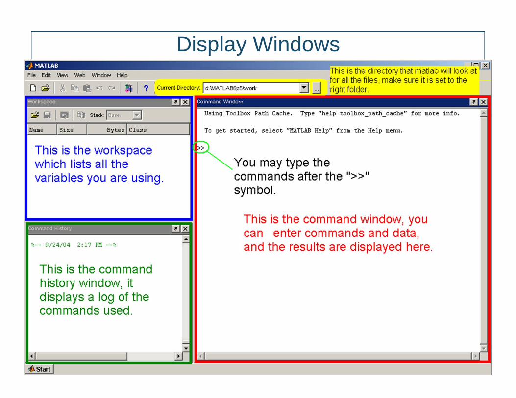
3. MATLAB Environment: 1. the command window, where you will type commands; 2. the command history, which keeps a list of commands that have been used; and 3. the workspace, where the variables used are kept.


6

4. Your first command on the command window should be to change to your data directory where you will keep your work.

You can do this in the command window by using the command CD (change directory) followed by the desired directory.

It is also important to use the command clear all and clf to clear all previous variables in memory and all figures.

5. Help is available in several forms in MATLAB.

6. To type your scripts or functions you can use the editor provided by MATLAB; simply type edit.

Creating Vectors and Matrices


7

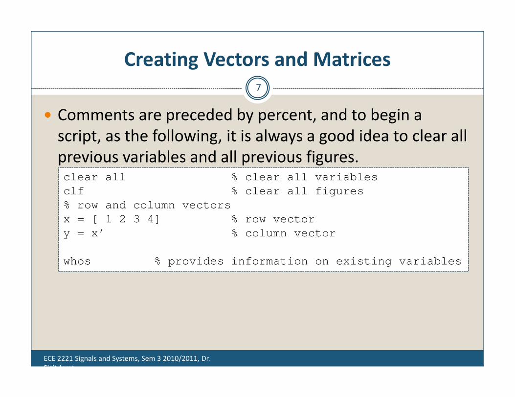
Comments are preceded by percent, and to begin a script, as the following, it is always a good idea to clear all previous variables and all previous figures.clear all % clear all variablesclf % clear all figures% row and column vectorsx = [ 1 2 3 4] % row vectory = x’ % column vector

whos % provides information on existing variables


8

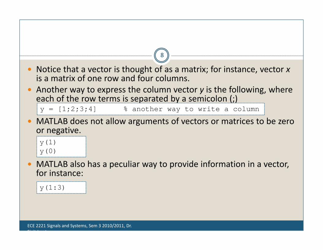
Notice that a vector is thought of as a matrix; for instance, vector x is a matrix of one row and four columns.

Another way to express the column vector y is the following, where each of the row terms is separated by a semicolon (;)

MATLAB does not allow arguments of vectors or matrices to be zero or negative.

MATLAB also has a peculiar way to provide information in a vector, for instance:

y = [1;2;3;4] % another way to write a column

y(1)y(0)

y(1:3)


9

Matrices are constructed as an concatenation of rows (or columns):

To create a vector corresponding to a sequence of numbers (in this case integers) there are different approaches,

A = [ 1 2; 3 4; 5 6] % matrix A with rows [1 2], [3 4] and [5 6]

n = 0:10 % vector with entries 0 to 10 increased by 1n = [0:10]n1 = 0:2:10 % vector with entries from 0 to 10 increased by 2nn1 = [n n1] % combination of vectors

Vectorial Operations


10

The solution of a set of linear equations is very simple in MATLAB. To guarantee that a unique solution exists, the determinant of the matrix should

be computed before inverting the matrix. If the determinant is zero MATLAB will indicate the solution is not possible.

z = 3x % multiplication by a constantv = x.x % multiplication of entries of two vectorsw = xx’ % multiplication of x (row vector) by x’(column vector)

A = [1 0 0; 2 2 0; 3 3 3]; % 3x3 matrixt = det(A); % MATLAB function that calculates determinantb = [2 2 2]’; % column vectorx = inv(A)b; % MATLAB function that inverts a matrixdisp(’ Ax = b’) % MATLAB function that displays the text in ’ ’

%Another way to solve this set of equations isx = b’/A’


11

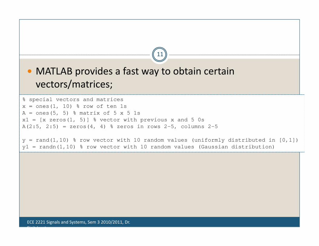
MATLAB provides a fast way to obtain certain vectors/matrices;

% special vectors and matricesx = ones(1, 10) % row of ten 1sA = ones(5, 5) % matrix of 5 x 5 1sx1 = [x zeros(1, 5)] % vector with previous x and 5 0sA(2:5, 2:5) = zeros(4, 4) % zeros in rows 2-5, columns 2-5

y = rand(1,10) % row vector with 10 random values (uniformly distributed in [0,1])y1 = randn(1,10) % row vector with 10 random values (Gaussian distribution)

Using Built‐In Functions


12

MATLAB provides a large number of built‐in functions. The following script uses some of them.

To learn about any of these functions use help.% using built‐in functionst = 0:0.01:1; % time vector from 0 to 1 with interval of 0.01x = cos(2pit/0.1); % cos processes each of the entries in% vector t to get the corresponding value in vector x% plotting the function xfigure(1) % numbers the figureplot(t, x) % interpolated continuous plotxlabel(’t (sec)’) % label of x‐axisylabel(’x(t)’) % label of y‐axis% let’s hear itsound(1000x, 10000)


13

To illustrate the plotting and the sound routines, let us create a chirp that is a sinusoid for which the frequency is varying with time.

Other built‐in functions are sin, tan, acos, asin, atan, atan2, log, log10, exp, etc. Find out what each does using help and obtain a listing of all the functions in the signal processing toolbox.

y = sin(2pit.ˆ2/.1); % no ce the dot in the squaring% t was defined beforesound(1000y, 10000) % to listen to the sinusoidfigure(2) % numbering of the figureplot(t(1:100), y(1:100)) % plotting of 100 values of yfigure(3)plot(t(1:100), x(1:100), ’k’, t(1:100), y(1:100), ’r’) % plotting x and y on same plot

Creating Your Own Functions


14

MATLAB has created a lot of functions to make our lives easier, and it allows us also to create—in the same way—our own.

The following file is for a function f with an input of a scalar x and output of a scalar y related by a mathematical function:

A function is created using the word “function” and then defining the output (y), the name of the function ( f ), and the input of the function (x), followed by lines of code defining the function, which in this case is given by the second line.

Functions cannot be executed on their own—they need to be part of a script. If you try to execute the above function MATLAB will give the following:

function y = f(x)y = x+exp(‐sin(x))/(1 + xˆ2);

??? format compact;function y = f(x)

Error: A function declaration cannot appear within a script M‐file.


15

To compute the value of the function for a vector as input, we compute for each of the values in the vector the corresponding output using a for loop as shown in the following.

x = 0:0.1:100; % create an input vector xN = length(x); % find the length of xy = zeros(1,N); % initialize the output y to zerosfor n = 1:N, % for the variable n from 1 to N, computey(n) = f(x(n)); % the functionendfigure(3)plot(x, y)grid % put a grid on the figuretitle(’Function f(x)’)xlabel(’x’)ylabel(’y’)

This is not very efficient. A general rule in MATLAB is: ‐ Loops are to be avoided, and ‐ vectorial computations are encouraged.


16

A general rule in MATLAB is: Loops are to be avoided, and vectorialcomputations are encouraged.

function yy = ff(x)% vectorial functionyy = x.exp(‐sin(x))./(1 + x);

z = ff(x); % x defined before,% z instead of yy is the output of the function fffigure(4)plot(x, z); gridtitle(’Function ff(x)’) % MATLAB function that puts title in plotxlabel(’x’) % MATLAB function to label x‐axisylabel(’z’) % MATLAB function to label y‐axis

stem(x(1:30), z(1:30))gridtitle(’Function ff(x)’)xlabel(’x’)ylabel(’z’)

Saving and Loading Data


17

In many situations you would like to either save some data or load some data. The following is one way to do it.

Suppose you want to build and save a table of sine values for angles between 0 and 360 degrees in intervals of 3 degrees. This can be done as follows:

To load the table, we use the function load with the name given to the saved table “sine” (the extension

*.mat is not needed). The following script illustrates this:

x = 0:3:360;y = sin(xpi/180); % sine computes the argument in radiansxy = [x’ y’]; % vector with 2 columns one for x’% and another for y’

save sine.mat xy

clear allload sinewhos


18

Finally, MATLAB provides some data files for experimentation and you only need to load them.

The following “train.mat” is the recording of a train whistle, sampled at the rate of Fs samples/sec, which accompanies the sampled signal y(n)clear allload trainwhos

sound(y, Fs)plot(y)


19

MATLAB also provides two‐dimensional signals, or images, such as “clown.mat,” a 200 320 pixels image.clear allload clownwhos

% We can display this image in gray levelscolormap(’gray’)imagesc(X)

% Or in color usingcolormap(’hot’)imagesc(X)

Symbolic Computations


20

We have considered the numerical capabilities of MATLAB, by which numerical data are transformed into numerical data.

There will be many situations when we would like to do algebraic or calculus operations resulting in terms of variables rather than numerical data.

For instance, we might want to find a formula to solve quadratic algebraic equations, to find a difficult integral, or to obtain the Laplace or the Fourier transform of a signal.

For those cases MATLAB provides the Symbolic Math Toolbox, which uses the interface between MATLAB and MAPLE, a symbolic computing system.


21

clf; clear all% symbolicsyms t y z % define the symbolic variablesy = cos(tˆ2) % chirp signal ‐‐ no ce no . before ˆ since t is no vectorz = diff(y) % derivativefigure(1)subplot(211)ezplot(y, [0, 2pi]);grid % plotting for symbolic y between 0 and 2pihold onsubplot(212)ezplot(z, [0, 2pi]);gridhold on%numericTs = 0.1; % sampling periodt1 = 0:Ts:2pi; % sampled timey1 = cos(t1.ˆ2); % sampled signal ‐‐notice difference with y abovez1 = diff(y1)./diff(t1); % difference ‐‐ approximation to derivativefigure(1)subplot(211)stem(t1, y1, ’r’);axis([0 2pi 1.1min(y1) 1.1max(y1)])subplot(212)stem(t1(1:length(y1) ‐ 1), z1, ’r’);axis([0 2pi 1.1min(z1) 1.1max(z1)])legend(’Derivative (black)’,’Difference (blue)’)hold off

Ramp, Unit‐Step, and Impulse Responses


22

We illustrate the response of a linear system represented by a differential equation,

clear all; clfsyms y t x z% input a unit‐step (heaviside) responsey = dsolve(’D2y + 5*Dy + 6y = heaviside(t)’,’y(0) = 0’,’Dy(0) = 0’,’t’);x = diff(y); % impulse responsez = int(y); % ramp responsefigure(1)subplot(311)ezplot(y, [0,5]);title(’Unit‐step response’)subplot(312)ezplot(x, [0,5]);title(’Impulse response’)subplot(313)ezplot(z, [0,5]);title(’Ramp response’)

Basic Numeric and Symbolic MATLAB Functions


23

MATLAB Assignment


24

Reference: Engineering Problem Solving Using MATLAB, by Professor Gary Ford, University of California, Davis.

Topics

ECE 2221 Signals and Systems

26

Introduction MATLAB Environment Getting Help Variables Vectors, Matrices, and Linear Algebra Mathematical Functions and Applications Plotting Selection Programming M-Files User Defined Functions Specific Topics

Introduction


27

What is MATLAB ?• MATLAB is a computer program that combines computation and

visualization power that makes it particularly useful tool for engineers.

• MATLAB is an executive program, and a script can be made with a list of MATLAB commands like other programming language.

MATLAB Stands for MATrix LABoratory.• The system was designed to make matrix computation particularly easy.

The MATLAB environment allows the user to:• manage variables• import and export data• perform calculations• generate plots• develop and manage files for use with MATLAB.

MATLABEnvironment

To start MATLAB: START PROGRAMS

MATLAB 6.5 MATLAB 6.5Or shortcut creation/activation

on the desktop

ECE 2221 Signals and Systems 28


Display Windows

Display Windows (con’t…)


30

Graphic (Figure) Window Displays plots and graphs Created in response to graphics commands.

M-file editor/debugger window Create and edit scripts of commands called M-files.

Getting Help


31

type one of following commands in the command window: help – lists all the help topic help topic – provides help for the specified topic help command – provides help for the specified command

help help – provides information on use of the help command helpwin – opens a separate help window for navigation lookfor keyword – Search all M-files for keyword

Getting Help (con’t…)


32

Google “MATLAB helpdesk” Go to the online HelpDesk provided by

www.mathworks.com

You can find EVERYTHING you need to know about MATLAB from the online HelpDesk.

Variables


33

Variable names: Must start with a letter May contain only letters, digits, and the underscore “_” Matlab is case sensitive, i.e. one & OnE are different variables. Matlab only recognizes the first 31 characters in a variable name.

Assignment statement: Variable = number; Variable = expression;

Example:>> tutorial = 1234;>> tutorial = 1234tutorial =

1234

NOTE: when a semi‐colon ”;” is placed at the end of each command, the result is not displayed.

Variables (con’t…)


34 Special variables: ans : default variable name for the result pi: = 3.1415926………… eps: = 2.2204e-016, smallest amount by which 2 numbers can differ.

Inf or inf : , infinity NaN or nan: not-a-number

Commands involving variables: who: lists the names of defined variables whos: lists the names and sizes of defined variables clear: clears all varialbes, reset the default values of special variables. clear name: clears the variable name clc: clears the command window clf: clears the current figure and the graph window.

Vectors, Matrices and Linear Algebra


35

Vectors Array Operations Matrices Solutions to Systems of Linear Equations.

Vectors


36

A row vector in MATLAB can be created by an explicit list, starting with a left bracket, entering the values separated by spaces (or commas) and closing the vector with a right bracket.

A column vector can be created the same way, and the rows are separated by semicolons. Example:

>> x = [ 0 0.25*pi 0.5*pi 0.75*pi pi ]x =

0 0.7854 1.5708 2.3562 3.1416>> y = [ 0; 0.25*pi; 0.5*pi; 0.75*pi; pi ]y =

00.78541.57082.35623.1416

x is a row vector.

y is a column vector.

Vectors (con’t…)


37

Vector Addressing – A vector element is addressed in MATLAB with an integer index enclosed in parentheses.

Example:>> x(3)ans =

1.5708

1st to 3rd elements of vector x

The colon notation may be used to address a block of elements.(start : increment : end)

start is the starting index, increment is the amount to add to each successive index, and end is the ending index. A shortened format (start : end) may be used if increment is 1.

Example:>> x(1:3)ans =

0 0.7854 1.5708

NOTE: MATLAB index starts at 1.

3rd element of vector x

Vectors (con’t…)


38

Some useful commands:

x = start:end create row vector x starting with start, counting by one, ending at end

x = start:increment:end create row vector x starting with start, counting by increment, ending at or before end

linspace(start,end,number) create row vector x starting with start, ending at end, having number elements

length(x) returns the length of vector x

y = x’ transpose of vector x

dot (x, y) returns the scalar dot product of the vector x and y.

The format function


39

format short 1.3333 0.0000 format short 1.3333e+000 1.2345e‐006 format short g 1.3333 1.2345e‐006 format long 1.33333333333333

0.00000123450000 format long e 1.333333333333333e+000

1.234500000000000e‐006 format long g 1.33333333333333

1.2345e‐006 format bank 1.33 0.00 format rat 4/3 1/810045 format hex 3ff5555555555555

3eb4b6231abfd271

Array Operations


40

Scalar-Array MathematicsFor addition, subtraction, multiplication, and division of an array by a

scalar simply apply the operations to all elements of the array. Example:

>> f = [ 1 2; 3 4]f =

1 23 4

>> g = 2*f – 1g =

1 35 7

Each element in the array f is multiplied by 2, then subtracted by 1.

Array Operations (con’t…)


41

Element-by-Element Array-Array Mathematics.

Operation Algebraic Form MATLAB

Addition a + b a + b

Subtraction a – b a – b

Multiplication a x b a .* b

Division a b a ./ b

Exponentiation ab a .^ b

Example:>> x = [ 1 2 3 ];>> y = [ 4 5 6 ];>> z = x .* yz =

4 10 18

Each element in x is multiplied by the corresponding element in y.

Matrices

A is an m x n matrix.


A Matrix array is two-dimensional, having both multiple rows and multiple columns, similar to vector arrays: it begins with [, and end with ] spaces or commas are used to separate elements in a row semicolon or enter is used to separate rows.

•Example:>> f = [ 1 2 3; 4 5 6]f =

1 2 34 5 6

>> h = [ 2 4 61 3 5]h =

2 4 61 3 5the main diagonal

Matrices (con’t…)


43

Matrix Addressing:-- matrixname(row, column)-- colon may be used in place of a row or column reference to select

the entire row or column.

recall:f =

1 2 34 5 6

h =2 4 61 3 5

Example:

>> f(2,3)

ans =

6

>> h(:,1)

ans =

2

1

Generating Basic Matrices and Load function


44

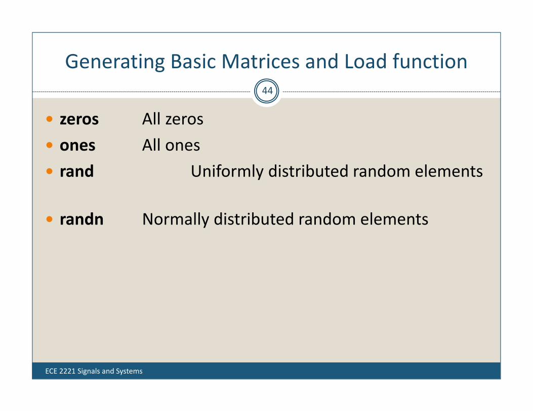
zeros All zeros ones All ones rand Uniformly distributed random elements

randn Normally distributed random elements



45

Some useful commands:

zeros(n)zeros(m,n)

ones(n)ones(m,n)

size (A)

length(A)

returns a n x n matrix of zerosreturns a m x n matrix of zeros

returns a n x n matrix of onesreturns a m x n matrix of ones

for a m x n matrix A, returns the row vector [m,n] containing the number of rows and columns in matrix.

returns the larger of the number of rows or columns in A.



46

Transpose B = A’

Identity Matrix eye(n) returns an n x n identity matrixeye(m,n) returns an m x n matrix with ones on the main diagonal and zeros elsewhere.

Addition and subtraction C = A + BC = A – B

Scalar Multiplication B = A, where is a scalar.

Matrix Multiplication C = A*B

Matrix Inverse B = inv(A), A must be a square matrix in this case.rank (A) returns the rank of the matrix A.

Matrix Powers B = A.^2 squares each element in the matrixC = A * A computes A*A, and A must be a square matrix.

Determinant det (A), and A must be a square matrix.

more commands

A, B, C are matrices, and m, n, are scalars.

Solutions to Systems of Linear Equations


47

Example: a system of 3 linear equations with 3 unknowns (x1, x2, x3):3x1 + 2x2 – x3 = 10-x1 + 3x2 + 2x3 = 5x1 – x2 – x3 = -1

Then, the system can be described as:

Ax = b

111231123

A

3

2

1

xxx

x

15

10b

Let :

Solutions to Systems of Linear Equations (con’t…)


48 Solution by Matrix Inverse:

Ax = bA-1Ax = A-1bx = A-1b

MATLAB:>> A = [ 3 2 -1; -1 3 2; 1 -1 -1];>> b = [ 10; 5; -1];>> x = inv(A)*bx =

-2.00005.0000-6.0000

Answer:x1 = -2, x2 = 5, x3 = -6

Solution by Matrix Division:The solution to the equation

Ax = bcan be computed using left division.

Answer:x1 = -2, x2 = 5, x3 = -6

NOTE: left division: A\b b A right division: x/y x y

MATLAB:>> A = [ 3 2 -1; -1 3 2; 1 -1 -1];>> b = [ 10; 5; -1];>> x = A\bx =

-2.00005.0000-6.0000

Matrices


49

Entering Matrices Magic Sum Diag Transpose Subscripts Colon Operator

Load function and Concatenation

Load Is used to load any matrix or data points in matlab Usage

Load magic.dat

Concatenation Create 3X3 matrix A Create 3X2 matrix B Create 2X5 matrix C Concatenate


Mathematical Functions and Applications


51

Signal Representations, and Processing Polynomials Partial Fraction Expansion

Signal Representations, and Processing(Lab Exercise)


52

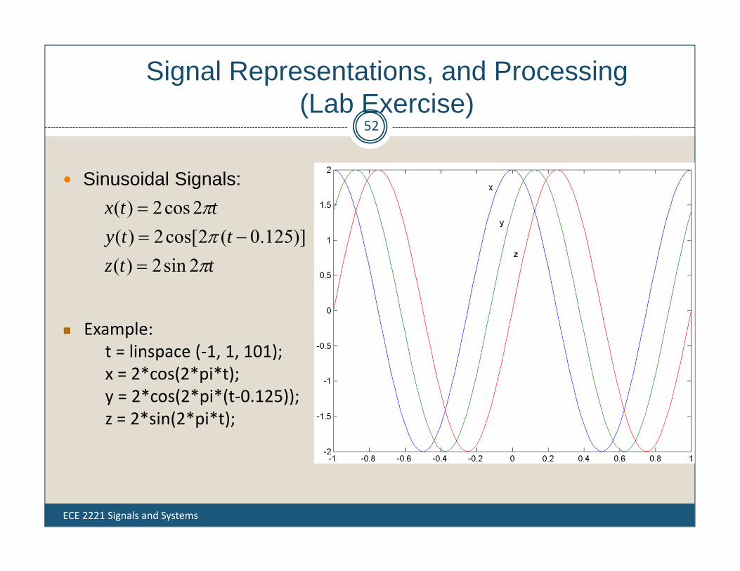
Sinusoidal Signals:

ttztty

ttx

2sin2)()]125.0(2cos[2)(

2cos2)(

Example:t = linspace (‐1, 1, 101);x = 2*cos(2*pi*t);y = 2*cos(2*pi*(t‐0.125));z = 2*sin(2*pi*t);

Polynomials


53

The polynomials are represented by their coefficients in MATLAB. Consider the following polynomial:

A(s) = s3 + 3s2 + 3s + 1 For s is scalar: use scalar operations A = s^3 + 3*s^2 + 3*s + 1;

For s is a vector or a matrix: use array or element by element operation A = s.^3 + 3*s.^2 + 3.*s + 1;

function polyval(a,s): evaluates a polynomial with coefficients in vector a for the values in s.

Lab Exercise


54

Example:>> s = linspace (-5, 5, 100);>> coeff = [ 1 3 3 1];>> A = polyval (coeff, s);>> plot (s, A),>> xlabel ('s')>> ylabel ('A(s)')

A(s) = s3 + 3s2 + 3s + 1

Polynomials (con’t…)


55

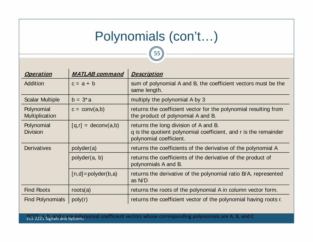
Operation MATLAB command Description

Addition c = a + b sum of polynomial A and B, the coefficient vectors must be the same length.

Scalar Multiple b = 3*a multiply the polynomial A by 3

Polynomial Multiplication

c = conv(a,b) returns the coefficient vector for the polynomial resulting from the product of polynomial A and B.

Polynomial Division

[q,r] = deconv(a,b) returns the long division of A and B.q is the quotient polynomial coefficient, and r is the remainder polynomial coefficient.

Derivatives polyder(a) returns the coefficients of the derivative of the polynomial A

polyder(a, b) returns the coefficients of the derivative of the product of polynomials A and B.

[n,d]=polyder(b,a) returns the derivative of the polynomial ratio B/A, represented as N/D

Find Roots roots(a) returns the roots of the polynomial A in column vector form.

Find Polynomials poly(r) returns the coefficient vector of the polynomial having roots r.

NOTE: a, b, and c are polynomial coefficient vectors whose corresponding polynomials are A, B, and C

Partial Fraction Expansion (PFE)


56

n

nrs

crs

crs

csH

...)(2

2

1

1

)()()(

sAsBsH , where B(s) and A(s) are polynomials.

H(s) can also be represented in the following form:

Lab Exercise


57

MATLAB:>> b = [ 1 2];>> a = [ 1 4 3 0];>> [c,r] = residue (b, a)c =‐0.1667‐0.50000.6667

r =‐3‐10

Example (Distinct Real Roots):

3

3

2

2

1

123 034

2)(rs

crs

crs

csss

ssH

NOTE: a zero is needed in the coefficient vector to represent the constant 0.

c1c2c3

r1r2r3

ssssH 3/2

12/1

36/1)(

Answer:

Plotting

For more information on 2-D plotting, type help graph2d Plotting a point:

>> plot ( variablename, ‘symbol’)

command description

axis ([xmin xmax ymin ymax]) Define minimum and maximum values of the axes

axis square Produce a square plot

axis equal equal scaling factors for both axes

axis normal turn off axis square, equal

axis (auto) return the axis to defaults


the function plot () creates a graphics window, called a Figure window, and named by default “Figure No. 1”

Example : Complex number>> z = 1 + 0.5j;>> plot (z, ‘.’)

commands for axes:

Plotting (con’t…) Plotting Curves:

plot (x,y) – generates a linear plot of the values of x (horizontal axis) and y (vertical axis). semilogx (x,y) – generate a plot of the values of x and y using a logarithmic scale for x and a

linear scale for y semilogy (x,y) – generate a plot of the values of x and y using a linear scale for x and a logarithmic

scale for y. loglog(x,y) – generate a plot of the values of x and y using logarithmic scales for both x and y

Multiple Curves: plot (x, y, w, z) –multiple curves can be plotted on the same graph by using multiple arguments in a plot command. The

variables x, y, w, and z are vectors. Two curves will be plotted: y vs. x, and z vs. w. legend (‘string1’, ‘string2’,…) – used to distinguish between plots on the same graph

exercise: type help legend to learn more on this command.

Multiple Figures: figure (n) – used in creation of multiple plot windows. place this command before the plot() command, and the

corresponding figure will be labeled as “Figure n” close – closes the figure n window. close all – closes all the figure windows.

Subplots: subplot (m, n, p) – m by n grid of windows, with p specifying the current plot as the pth window


Lab Exercise


60

Example: (polynomial function)plot the polynomial using linear/linear scale, log/linear scale, linear/log scale, & log/log scale:

y = 2x2 + 7x + 9

% Generate the polynomial:x = linspace (0, 10, 100);y = 2*x.^2 + 7*x + 9;

% plotting the polynomial:figure (1);subplot (2,2,1), plot (x,y);title ('Polynomial, linear/linear scale');ylabel ('y'), grid;subplot (2,2,2), semilogx (x,y);title ('Polynomial, log/linear scale');ylabel ('y'), grid;subplot (2,2,3), semilogy (x,y);title ('Polynomial, linear/log scale');xlabel('x'), ylabel ('y'), grid;subplot (2,2,4), loglog (x,y);title ('Polynomial, log/log scale');xlabel('x'), ylabel ('y'), grid;


Plotting (con’t…)

Plotting (con’t…)

Adding new curves to the existing graph: Use the hold command to add lines/points to an existing plot.

hold on – retain existing axes, add new curves to current axes. Axes are rescaled when necessary.

hold off – release the current figure window for new plots

Command Description

grid on Adds dashed grids lines at the tick marks

grid off removes grid lines (default)

grid toggles grid status (off to on, or on to off)

title (‘text’) labels top of plot with text in quotes

xlabel (‘text’) labels horizontal (x) axis with text is quotes

ylabel (‘text’) labels vertical (y) axis with text is quotes

text (x,y,’text’) Adds text in quotes to location (x,y) on the current axes, where (x,y) is in units from the current plot.


Grids and Labels:

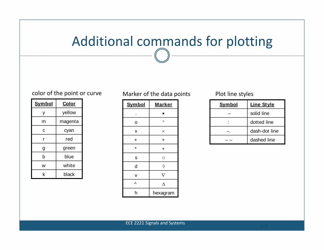
Additional commands for plotting

Symbol Color

y yellow

m magenta

c cyan

r red

g green

b blue

w white

k black

Symbol Marker

.

o

x

+ +

*

s □

d ◊

v

^

h hexagram

Symbol Line Style

– solid line

: dotted line

–. dash-dot line

– – dashed line


color of the point or curve Marker of the data points Plot line styles

Selection Programming


64

Flow Control Loops

Flow Control


65

Simple if statement:if logical expression

commandsend

Example: (Nested)if d <50

count = count + 1;disp(d);if b>d

b=0;end

end Example: (else and elseif clauses)

if temperature > 100disp (‘Too hot – equipment malfunctioning.’)

elseif temperature > 90disp (‘Normal operating range.’);

elseif (‘Below desired operating range.’)else

disp (‘Too cold – turn off equipment.’)end

Flow Control (con’t…)


66

The switch statement:switch expression

case test expression 1commands

case test expression 2commands

otherwisecommands

end Example:

switch interval < 1case 1

xinc = interval /10;case 0

xinc = 0.1;end

Loops


67

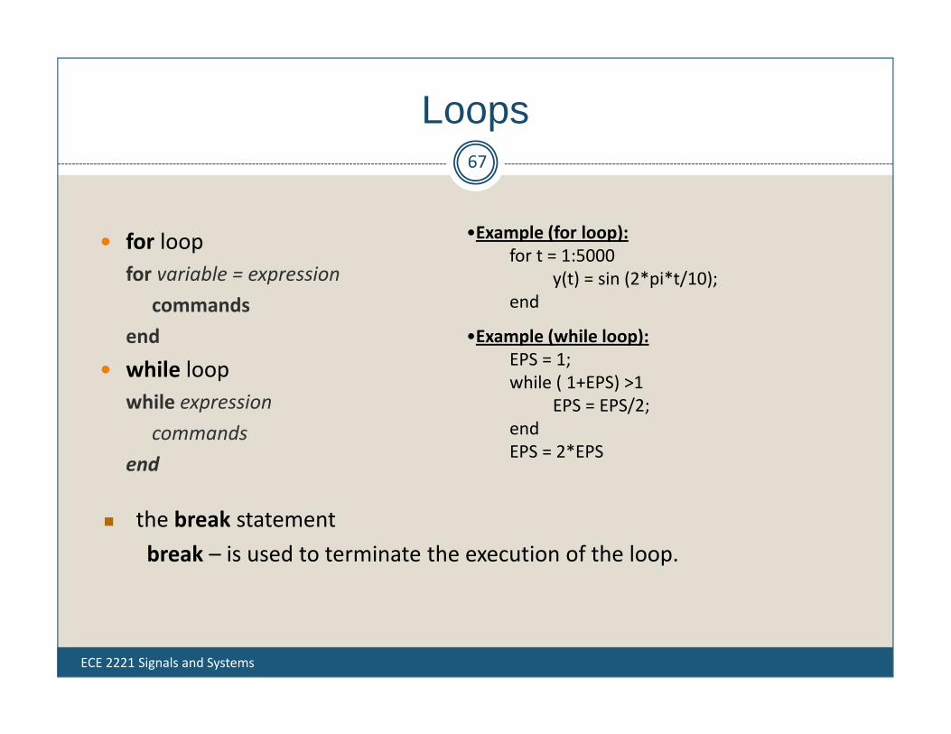
for loopfor variable = expression

commandsend

while loopwhile expression

commandsend

•Example (for loop):for t = 1:5000

y(t) = sin (2*pi*t/10);end

•Example (while loop):EPS = 1;while ( 1+EPS) >1

EPS = EPS/2;endEPS = 2*EPS

the break statementbreak – is used to terminate the execution of the loop.

M-Files


68

The M-file is a text file that consists a group of MATLAB commands.

MATLAB can open and execute the commands exactly as if they were entered at the MATLAB command window.

To run the M-files, just type the file name in the command window. (make sure the current working directory is set correctly)

All MATLAB commands are M-files.

So far, we have executed the commands in the command window. But a more practical way is to create a M‐file.

Lab Exercise


69

Use the following and create an a Matlab file % Generate the polynomial:x = linspace (0, 10, 100);y = 2*x.^2 + 7*x + 9;


User‐Defined Function


70

Add the following command in the beginning of your m‐file:function [output variables] = function_name (input variables);

NOTE: the function_name should be the same as your file name to avoid confusion.

calling your function:‐‐ a user‐defined function is called by the name of the m‐file, not the name given in the function definition.‐‐ type in the m‐file name like other pre‐defined commands.

Comments:‐‐ The first few lines should be comments, as they will be displayed if help is requested for the function name. the first comment line is reference by the lookfor command.

Lab Exercise


71

Create the following m file calledfunction [y]=poly2ord(x)y = 2*x.^2 + 7*x + 9;

Save the file

In the command window execute >> poly2ord >> poly2ord(2)

NOTE: the function_name should be the same as your file name to avoid confusion.

Lab Exercise


72

Change the previous program as follows:% Generate the polynomial:x = linspace (0, 10, 100);y = poly2ord(x);


Specific Topics


73

This tutorial gives you a general background on the usage of MATLAB.

There are thousands of MATLAB commands for many different applications, therefore it is impossible to cover all topics here.

For a specific topic relating to a class, you should consult the TA or the Instructor.

Signal Implementation with MATLAB

Signal Implementation with MATLAB (Part a)

55)8cos()2sin(5)(1 tfortttx

Signal implementation with MATLAB (Part b)

1010)2sin(5)( 2.01 tfortetx t

Signal implementation with MATLAB (Part c)

2010)4/31.0sin(92.0)(1 kforktx

Computer Assignment #1


781. Plot the following signals CT using Matlab: (hint: help sign)1. Unit step function2. Unit impulse function3. A rectangular pulse of width 24. Unit ramp function

2. Plot the following signals using Matlab1. u(t-1)2. u(2t+1)3. delta(t-2.5)4. r(t-3)

3. Plot a 50 Hz sinusoidal signal sin(2*pi*f*t) sampled at 600 Hz.

This assignment is group work, 1 group consist of max 3 members.

Upload the softcopy to the drop box of ECE2221 e-learning Submit the hardcopy to my office by 28.01.2011, 12.00PM.

ECE 2221 SIGNALS AND SYSTEMS - staff.iium.edu.mystaff.iium.edu.my/sigit/ece2221/pdf/05 Matlab for...

Documents

Transcript of ECE 2221 SIGNALS AND SYSTEMS - staff.iium.edu.mystaff.iium.edu.my/sigit/ece2221/pdf/05 Matlab for...