EC3201 - Teoría Macroeconómica 2 - Randall Romero
113
Dynamic programming Randall Romero Aguilar, PhD EC3201 - Teoría Macroeconómica 2 II Semestre 2019 Last updated: November 14, 2019
Transcript of EC3201 - Teoría Macroeconómica 2 - Randall Romero

Dynamic programming
Randall Romero Aguilar, PhD
EC3201 - Teoría Macroeconómica 2II Semestre 2019
Last updated: November 14, 2019

Table of contents
1. Introduction
2. Basics of dynamic programming
3. Consumption and financial assets: infinite horizon
4. Consumption and financial assets: finite horizon
5. Consumption and physical investment
6. The McCall job search model

1. Introduction

About this lecture
I We study how to use Bellman equations to solve dynamicprogramming problems.
I We consider a consumer who wants to maximize his lifetimeconsumption over an infinite horizon, by optimally allocatinghis resources through time. Two alternative models:
1. the consumer uses a financial instrument (say a bank depositwithout overdraft limit) to smooth consumption;
2. the consumer has access to a production technology and usesthe level of capital to smooth consumption.
I To keep matters simple, we assume:I a logarithmic instant utility function;I there is no uncertainty.
I To start, we review some math that we’ll need later.
©Randall Romero Aguilar, PhD EC-3201 / 2019.II 1

Static optimization
I Optimization is a predominant theme in economic analysis.I For this reason, the classical calculus methods of finding free
and constrained extrema occupy an important place in theeconomist’s everyday tool kit.
I Useful as they are, such tools are applicable only to staticoptimization problems.
I The solution sought in such problems usually consists of asingle optimal magnitude for every choice variable.
I It does not call for a schedule of optimal sequential action.
©Randall Romero Aguilar, PhD EC-3201 / 2019.II 2

Dynamic optimization
I In contrast, a dynamic optimization problem poses thequestion of what is the optimal magnitude of a choice variablein each period of time within the planning period.
I It is even possible to consider an infinite planning horizon.I The solution of a dynamic optimization problem would thus
take the form of an optimal time path for every choicevariable, detailing the best value of the variable today,tomorrow, and so forth, till the end of the planning period.
©Randall Romero Aguilar, PhD EC-3201 / 2019.II 3

Basic ingredients
A simple type of dynamic optimization problem would contain thefollowing basic ingredients:
1. a given initial point and a given terminal point;2. a set of admissible paths from the initial point to the terminal
point;3. a set of path values serving as performance indices (cost,
profit, etc.) associated with the various paths; and4. a specified objective-either to maximize or to minimize the
path value or performance index by choosing the optimal path.
©Randall Romero Aguilar, PhD EC-3201 / 2019.II 4

Alternative approaches to dynamic optimization
To find the optimal path, there are three major approaches:
Calculus of varia-tionsDating back to thelate 17th century,it works about vari-ations in the statepath.
Optimal controltheoryThe problem isviewed as havingboth a state anda control path,focusing on varia-tions of the controlpath.
Dynamic pro-grammingWhich embeds thecontrol problemin a family ofcontrol problems,focusing on theoptimal value ofthe problem (valuefunction).
©Randall Romero Aguilar, PhD EC-3201 / 2019.II 5

Salient features of dynamic optimization problems
I Although dynamic optimization is mostly couched in terms ofa sequence of time, it is also possible to envisage the planninghorizon as a sequence of stages in an economic process.
I In that case, dynamic optimization can be viewed as aproblem of multistage decision making.
I The distinguishing feature, however, remains the fact that theoptimal solution would involve more than one single value forthe choice variable.
©Randall Romero Aguilar, PhD EC-3201 / 2019.II 6

2. Basics of dynamic programming

The principle of optimality
The dynamic programming approach is based on the principle ofoptimality (Bellman, 1957)
An optimal policy has the property that, whatever the ini-tial state and decision are, the remaining decisions mustconstitute an optimal policy with regard to the state re-sulting from the first decision.
©Randall Romero Aguilar, PhD EC-3201 / 2019.II 7

Why dynamic programming?
Dynamic programming is a very attractive method for solvingdynamic optimization problems becauseI it offers backward induction, a method that is particularly
amenable to programmable computers, andI it facilitates incorporating uncertainty in dynamic optimization
models.
©Randall Romero Aguilar, PhD EC-3201 / 2019.II 8

Dynamic Programming: the basics
We now introduce basic ideas and methods of dynamicprogramming (Ljungqvist and Sargent 2004)I basic elements of a recursive optimization problemI the Bellman equationI methods for solving the Bellman equationI the Benveniste-Scheikman formula
©Randall Romero Aguilar, PhD EC-3201 / 2019.II 9
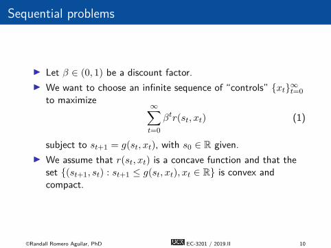
Sequential problems
I Let β ∈ (0, 1) be a discount factor.I We want to choose an infinite sequence of “controls” {xt}∞t=0
to maximize∞∑t=0
βtr(st, xt) (1)
subject to st+1 = g(st, xt), with s0 ∈ R given.I We assume that r(st, xt) is a concave function and that the
set {(st+1, st) : st+1 ≤ g(st, xt), xt ∈ R} is convex andcompact.
©Randall Romero Aguilar, PhD EC-3201 / 2019.II 10

Dynamic programming seeks a time-invariant policy function hmapping the state st into the control xt, such that the sequence{xt}∞t=0 generated by iterating the two functions
xt = h(st)
st+1 = g(st, xt)
starting from initial condition s0 at t = 0, solves the originalproblem. A solution in the form of equations is said to be recursive.
©Randall Romero Aguilar, PhD EC-3201 / 2019.II 11

To find the policy function h we need to know the value functionV (s), which expresses the optimal value of the original problem,starting from an arbitrary initial condition s ∈ S. Define
V (s0) = max{xt}∞t=0
∞∑t=0
βtr(st, xt)
subject to st+1 = g(st, xt), with s0 given.We do not know V (s0) until after we have solved the problem, butif we knew it the policy function h could be computed by solvingfor each s ∈ S the problem
maxx
{r(s, x) + βV (s′)
}, s.t. s′ = g(s, x) (2)
©Randall Romero Aguilar, PhD EC-3201 / 2019.II 12

Thus, we have exchanged the original problem of finding an infinitesequence of controls that maximizes expression (1) for the problemof finding the optimal value function V (s) and a function h thatsolves the continuum of maximum problems (2) —one maximumproblem for each value of s.The function V (s), h(s) are linked by the Bellman equation
V (s) = maxx
{r(s, x) + βV [g(s, x)]} (3)
The maximizer of the RHS is a policy function h(s) that satisfies
V (s) = r[s, h(s)] + βV {g[s, h(s)]} (4)
This is a functional equation to be solved for the pair of unknownfunctions V (s), h(s).
©Randall Romero Aguilar, PhD EC-3201 / 2019.II 13

Some properties
Under various particular assumptions about r and g, it turns outthat
1. The Bellman equation has a unique strictly concave solution.2. This solution is approached in the limit as j → ∞ by
iterations on
Vj+1(s) = maxx
{r(s, x) + βVj(s′)}, s.t. s′ = g(s, x), s given
starting from any bounded and continuous initial V0.3. There is a unique and time-invariant optimal policy of the
form xt = h(st), where h is chosen to maximize the RHS ofthe Bellman equation.
4. Off corners, the limiting value function V is differentiable.
©Randall Romero Aguilar, PhD EC-3201 / 2019.II 14

Side note:Banach Fixed-Point Theorem

Concave functions
I A real-valued function f on an interval (or, more generally, aconvex set in vector space) is said to be concave if, for any xand y in the interval and for any t ∈ [0, 1],
f((1− t)x+ ty) ≥ (1− t)f(x) + tf(y)
I A function is called strictly concave if
f((1− t)x+ ty) > (1− t)f(x) + tf(y)
for any t ∈ (0, 1) and x 6= y.
©Randall Romero Aguilar, PhD EC-3201 / 2019.II 15
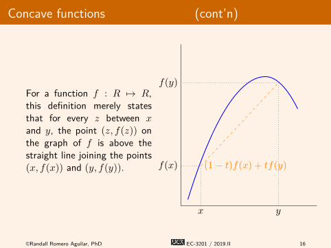
Concave functions (cont’n)
For a function f : R 7→ R,this definition merely statesthat for every z between xand y, the point (z, f(z)) onthe graph of f is above thestraight line joining the points(x, f(x)) and (y, f(y)).
x
f(x)
y
f(y)
(1− t)f(x) + tf(y)
©Randall Romero Aguilar, PhD EC-3201 / 2019.II 16

Fixed points
I A point x∗ is afixed-point of function fif it satisfies f(x∗) = x∗.
I Notice thatf(f(. . . f(x∗) . . . )) =x∗.
f
x
y = x
x∗0
x∗1
©Randall Romero Aguilar, PhD EC-3201 / 2019.II 17

Contraction mappings
A mapping f : X 7→ Xfrom a metric space X intoitself is said to be a strongcontraction with modulus δ,if 0 ≤ δ < 1 and
d(f(x), f(y)) ≤ δd(x, y)
for all x and y in X.
f
t
f(t)
|x− y|
|f(x)− f(y)|
x y
©Randall Romero Aguilar, PhD EC-3201 / 2019.II 18

Banach Fixed-Point Theorem
If f is a strong contraction on a metric space X, thenI it possesses an unique fixed-point x∗, that is f(x∗) = x∗
I if x0 ∈ X and xi+1 = f(xi), then the xi converge to x∗
Proof: Use x0 and x∗ in the definition of a strong contraction:
d(f(x0), f(x∗)) ≤ δd(x0, x∗) ⇒
d(x1, x∗) ≤ δd(x0, x∗) ⇒
d(xk, x∗) ≤ δkd(x0, x∗) → 0 as k → ∞
©Randall Romero Aguilar, PhD EC-3201 / 2019.II 19

Example 1:Searching a fixed point by functioniteration
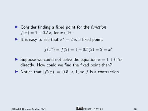
I Consider finding a fixed point for the functionf(x) = 1 + 0.5x, for x ∈ R.
I It is easy to see that x∗ = 2 is a fixed point:
f(x∗) = f(2) = 1 + 0.5(2) = 2 = x∗
I Suppose we could not solve the equation x = 1 + 0.5xdirectly. How could we find the fixed point then?
I Notice that |f ′(x)| = |0.5| < 1, so f is a contraction.
©Randall Romero Aguilar, PhD EC-3201 / 2019.II 20

By Banach Theorem, if we start from an arbitrary point x0 and byiteration we form the sequence xj+1 = f(xj), it follows thatlimj→∞ xj = x∗.
For example, pick:
x0 = 6
x1 = f(x0) = 1 + 62 = 4
x2 = f(x1) = 1 + 42 = 3
x3 = f(x2) = 1 + 32 = 2.5
x4 = f(x3) = 1 + 2.52 = 2.25
...
f
x
f(t)
x0
If we keep iterating, we will get arbitrarily close to the solutionx∗ = 2.
©Randall Romero Aguilar, PhD EC-3201 / 2019.II 21

First-order necessary condition
Starting with the Bellman equation
V (s) = maxx
{r(s, x) + βV [g(s, x)]}
Since the value function is differentiable, the optimal x∗ ≡ h(s)must satisfy the first-order condition
rx(s, x∗) + βV ′{g(s, x∗)}gx(s, x∗) = 0 (FOC)
©Randall Romero Aguilar, PhD EC-3201 / 2019.II 22
Envelope condition
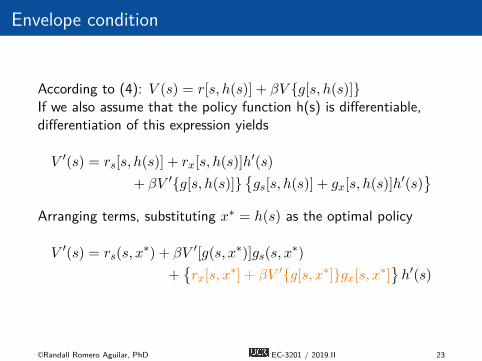
According to (4): V (s) = r[s, h(s)] + βV {g[s, h(s)]}If we also assume that the policy function h(s) is differentiable,differentiation of this expression yields
V ′(s) = rs[s, h(s)] + rx[s, h(s)]h′(s)
+ βV ′{g[s, h(s)]}{gs[s, h(s)] + gx[s, h(s)]h
′(s)}
Arranging terms, substituting x∗ = h(s) as the optimal policy
V ′(s) = rs(s, x∗) + βV ′[g(s, x∗)]gs(s, x
∗)
+{rx[s, x
∗] + βV ′{g[s, x∗]}gx[s, x∗]}h′(s)
©Randall Romero Aguilar, PhD EC-3201 / 2019.II 23

Envelope condition (cont’n)
The highlighted part cancels out because of (FOC), therefore
V ′(s) = rs(s, x∗) + βV ′ (s′) gs(s, x∗)
Notice that we could have obtained this result much faster bytaking derivative of
V (s) = r(s, x∗) + βV [g(s, x∗)]
with respect to the state variable s as if the control variablex∗ ≡ h(s) did not depend on s.
©Randall Romero Aguilar, PhD EC-3201 / 2019.II 24

Benveniste and Scheinkman formula
In the envelope condition
V ′(s) = rs(s, x∗) + βV ′ (s′) gs(s, x∗)
when the states and controls can be defined in such a way thatonly x appears in the transition equation, i.e.,
s′ = g(x) ⇒ gs(s, x∗) = 0,
the derivative of the value function becomes
V ′(s) = rs[s, h(s)] (B-S)
This is a version of a formula of Benveniste and Scheinkman.
©Randall Romero Aguilar, PhD EC-3201 / 2019.II 25
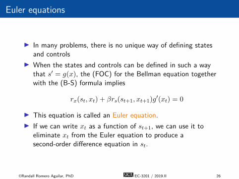
Euler equations
I In many problems, there is no unique way of defining statesand controls
I When the states and controls can be defined in such a waythat s′ = g(x), the (FOC) for the Bellman equation togetherwith the (B-S) formula implies
rx(st, xt) + βrs(st+1, xt+1)g′(xt) = 0
I This equation is called an Euler equation.I If we can write xt as a function of st+1, we can use it to
eliminate xt from the Euler equation to produce asecond-order difference equation in st.
©Randall Romero Aguilar, PhD EC-3201 / 2019.II 26
Solving the Bellman equation
I In those cases in which we want to go beyond the Eulerequation to obtain an explicit solution, we need to find thesolution V of the Bellman equation (3)
I Given V , it is straightforward to solve (3) successively tocompute the optimal policy.
I However, for infinite-horizon problems, we cannot usebackward iteration.
©Randall Romero Aguilar, PhD EC-3201 / 2019.II 27

Three computational methods
I There are three main types of computational methods forsolving dynamic programs. All aim to solve the BellmanequationI Guess and verifyI Value function iterationI Policy function iteration
I Each method is easier said than done: it is typicallyimpossible analytically to compute even one iteration.
I Usually we need computational methods for approximatingsolutions: pencil and paper are insufficient.
©Randall Romero Aguilar, PhD EC-3201 / 2019.II 28

Example 2:Computer solution of DP models

There are several computer programs available for solving dynamicprogramming models:I The CompEcon toolbox, a MATLAB toolbox accompanying
Miranda and Fackler (2002) textbook.I The PyCompEcon toolbox, my (still incomplete) Python
version of Miranda and Fackler toolbox.I Additional examples are available at quant-econ, a website by
Sargent and Stachurski with Python and Julia scripts.
©Randall Romero Aguilar, PhD EC-3201 / 2019.II 29

Guess and verify
I This method involves guessing and verifying a solution V tothe Bellman equation.
I It relies on the uniqueness of the solution to the equationI because it relies on luck in making a good guess, it is not
generally available.
©Randall Romero Aguilar, PhD EC-3201 / 2019.II 30
Value function iteration
I This method proceeds by constructing a sequence of valuefunctions and associated policy functions.
I The sequence is created by iterating on the following equation,starting from V0 = 0, and continuing until Vj has converged:
Vj+1(s) = maxx
{r(s, x) + βVj [g(s, x)]}
©Randall Romero Aguilar, PhD EC-3201 / 2019.II 31
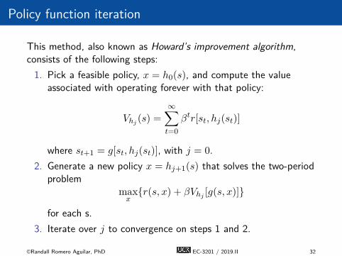
Policy function iteration
This method, also known as Howard’s improvement algorithm,consists of the following steps:
1. Pick a feasible policy, x = h0(s), and compute the valueassociated with operating forever with that policy:
Vhj(s) =
∞∑t=0
βtr[st, hj(st)]
where st+1 = g[st, hj(st)], with j = 0.2. Generate a new policy x = hj+1(s) that solves the two-period
problemmaxx
{r(s, x) + βVhj[g(s, x)]}
for each s.3. Iterate over j to convergence on steps 1 and 2.
©Randall Romero Aguilar, PhD EC-3201 / 2019.II 32
Stochastic control problems
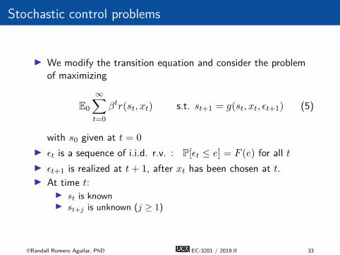
I We modify the transition equation and consider the problemof maximizing
E0
∞∑t=0
βtr(st, xt) s.t. st+1 = g(st, xt, ϵt+1) (5)
with s0 given at t = 0
I ϵt is a sequence of i.i.d. r.v. : P[ϵt ≤ e] = F (e) for all tI ϵt+1 is realized at t+ 1, after xt has been chosen at t.I At time t:
I st is knownI st+j is unknown (j ≥ 1)
©Randall Romero Aguilar, PhD EC-3201 / 2019.II 33

I The problem is to choose a policy or contingency planxt = h(st). The Bellman equation is
V (s) = maxx
{r(s, x) + β E[V
(s′)| s]
}I where s′ = g(s, x, ϵ),I and E{V (s′) |s} =
∫V (s′) dF (ϵ)
I The solution V (s) of the B.E. can be computed by valuefunction iteration.
©Randall Romero Aguilar, PhD EC-3201 / 2019.II 34

I The FOC for the problem is
rx(s, x) + β E{V ′ (s′) gx(s, x, ϵ) | s} = 0
I When the states and controls can be defined in such a waythat s does not appear in the transition equation,
V ′(s) = rs[s, h(s)]
I Substituting this formula into the FOC gives the stochasticEuler equation
rx(s, x) + β E{rs(s
′, x′)gx(s, x, ϵ) | s}= 0
©Randall Romero Aguilar, PhD EC-3201 / 2019.II 35

3. Consumption and financial assets: infinitehorizon

Consumption and financial assets
To ilustrate how dynamic programming works, we consider aintertemporal consumption problem.
©Randall Romero Aguilar, PhD EC-3201 / 2019.II 36

The consumer
I Planning horizon: infiniteI Instant utility depends on current consumption: u(ct)
I Constant utility discount rate β ∈ (0, 1)
I Lifetime utility is:
U(c0, c1, . . .) =
∞∑t=0
βtu(ct)
I The problem: choosing the optimal sequence of values {c∗t }that will maximize U , subject to a budget constraint.
©Randall Romero Aguilar, PhD EC-3201 / 2019.II 37

A savings model
The consumerI is endowed with A0 units of the consumption good,I does not have incomeI can save in a bank deposit, which yields a interest rate r.
The budget constraint is
At+1 = R(At − ct)
where R ≡ 1 + r is the gross interest rate.
©Randall Romero Aguilar, PhD EC-3201 / 2019.II 38

The value function
I Once he chooses the sequence {c∗t }∞t=0 of optimalconsumption, the maximum utility that he can achieved isultimately constraint only by his initial assets A0.
I So define the value function V as the maximum utility theconsumer can get as a function of his initial assets
V (A0) = max{ct,At+1}∞t=0
∞∑t=0
βtu(ct)
subject to At+1 = R(At − ct)
©Randall Romero Aguilar, PhD EC-3201 / 2019.II 39
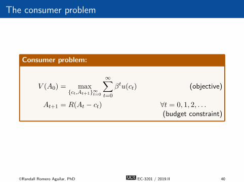
The consumer problem
Consumer problem:
V (A0) = max{ct,At+1}∞t=0
∞∑t=0
βtu(ct) (objective)
At+1 = R(At − ct) ∀t = 0, 1, 2, . . .(budget constraint)
©Randall Romero Aguilar, PhD EC-3201 / 2019.II 40

Dealing with the intertemporal budget constraintNotice that we have a budget constraint for every time period t.So we form the Lagrangean
V (A0) = max{ct,At+1}∞t=0
∞∑t=0
βtu(ct) +
∞∑t=0
λt[R(At − ct)−At+1]
= max{ct,At+1}∞t=0
∞∑t=0
{βtu(ct) + λt[R(At − ct)−At+1]
}Instead of dealing with the constraints explicitly, we can justsubstitute ct = At −At+1/R in all time periods:
= max{At+1}∞t=0
∞∑t=0
βtu
At −At+1
Rct
So, we choose consumption implicitly by choosing the path ofassets.©Randall Romero Aguilar, PhD EC-3201 / 2019.II 41
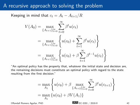
A recursive approach to solving the problemKeeping in mind that ct = At −At+1/R
V (A0) = max{At+1}∞t=0
∞∑t=0
βtu(ct)
= max{At+1}∞t=0
{u(c0) +
∞∑t=1
βtu(ct)
}
= max{At+1}∞t=0
{u(c0) + β
∞∑t=1
βt−1u(ct)
}“An optimal policy has the property that, whatever the initial state and decision are,the remaining decisions must constitute an optimal policy with regard to the stateresulting from the first decision.”
= maxA1
{u(c0) + β max
{At+2}∞t=0
∞∑t=0
βtu(ct+1)
}= max
A1
{u(c0) + βV (A1)}
©Randall Romero Aguilar, PhD EC-3201 / 2019.II 42
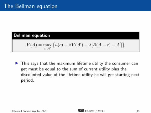
The Bellman equation
Bellman equation
V (A) = maxc, A′
{u(c) + βV (A′) + λ[R(A− c)−A′]
}
I This says that the maximum lifetime utility the consumer canget must be equal to the sum of current utility plus thediscounted value of the lifetime utility he will get starting nextperiod.
©Randall Romero Aguilar, PhD EC-3201 / 2019.II 43
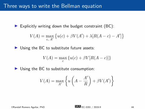
Three ways to write the Bellman equation
I Explicitly writing down the budget constraint (BC):
V (A) = maxc, A′
{u(c) + βV (A′) + λ[R(A− c)−A′]
}I Using the BC to substitute future assets:
V (A) = maxc
{u(c) + βV [R(A− c)]}
I Using the BC to substitute consumption:
V (A) = maxA′
{u
(A− A′
R
)+ βV (A′)
}
©Randall Romero Aguilar, PhD EC-3201 / 2019.II 44
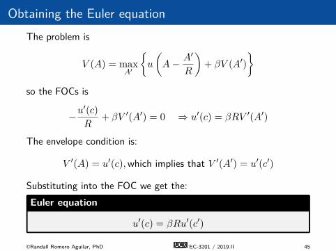
Obtaining the Euler equationThe problem is
V (A) = maxA′
{u
(A− A′
R
)+ βV (A′)
}so the FOCs is
−u′(c)
R+ βV ′(A′) = 0 ⇒ u′(c) = βRV ′(A′)
The envelope condition is:
V ′(A) = u′(c),which implies that V ′(A′) = u′(c′)
Substituting into the FOC we get the:Euler equation
u′(c) = βRu′(c′)
©Randall Romero Aguilar, PhD EC-3201 / 2019.II 45

Obtaining the Euler equation, second way
The Lagrangian for this problem is
V (A) = maxc, A′
{u(c) + βV (A′) + λ[R(A− c)−A′]
}so the FOCs are
u′(c) = λR
βV ′(A′) = λ
}⇒ u′(c) = βRV ′(A′)
and the envelope condition is
V ′(A) = λR = u′(c)
which implies that
V ′(A′) = u′(c′) ⇒ u′(c) = βRu′(c′)
©Randall Romero Aguilar, PhD EC-3201 / 2019.II 46

(Not quite) obtaining the Euler equation
The problem is
V (A) = maxc
{u(c) + βV [R(A− c)]}
so the FOCs isu′(c)− βRV ′(A′) = 0
but in this case the envelope condition is not useful:
V ′(A) = βRV ′(A′)
©Randall Romero Aguilar, PhD EC-3201 / 2019.II 47

The Euler equation
Euler equation
u′(c) = βRu′(c′)
I This says that at the optimum, if the consumer gets one moreunit of the good, he must be indifferent between consuming itnow (getting u′(c)) or saving it (which increases next-periodassets by R) an consuming it later, getting a discounted valueof βRu′(c′).
I Notice that this is the say result we found on Lecture 8(Applications of consumer theory), in the two-periodintertemporal consumption problem!
©Randall Romero Aguilar, PhD EC-3201 / 2019.II 48
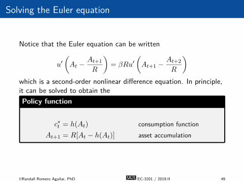
Solving the Euler equation
Notice that the Euler equation can be written
u′(At −
At+1
R
)= βRu′
(At+1 −
At+2
R
)which is a second-order nonlinear difference equation. In principle,it can be solved to obtain thePolicy function
c∗t = h(At) consumption functionAt+1 = R[At − h(At)] asset accumulation
©Randall Romero Aguilar, PhD EC-3201 / 2019.II 49

4. Consumption and financial assets: finitehorizon

The consumer
I Planning horizon: T (possibly infinite)I Instant utility depends on current consumption: u(ct) = ln ct
I Constant utility discount rate β ∈ (0, 1)
I Lifetime utility is:
U(c0, c1, . . . , cT ) =
T∑t=0
βt ln ct
I The problem: choosing the optimal values c∗t that willmaximize U , subject to a budget constraint.
©Randall Romero Aguilar, PhD EC-3201 / 2019.II 50
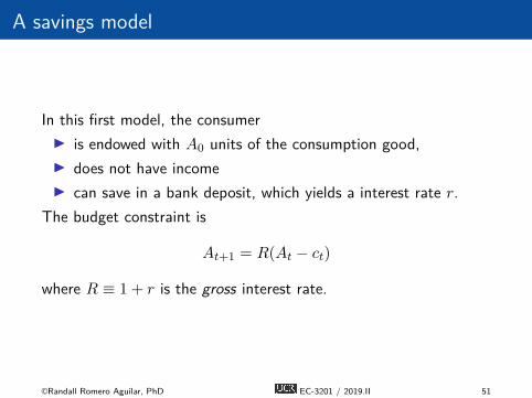
A savings model
In this first model, the consumerI is endowed with A0 units of the consumption good,I does not have incomeI can save in a bank deposit, which yields a interest rate r.
The budget constraint is
At+1 = R(At − ct)
where R ≡ 1 + r is the gross interest rate.
©Randall Romero Aguilar, PhD EC-3201 / 2019.II 51

The value function
I Once he chooses the sequence {c∗t }Tt=0 of optimalconsumption, the maximum utility that he can achieved isultimately constraint only by his initial assets A0 and by howmany periods he lives T + 1.
I So define the value function V as the maximum utility theconsumer can get as a function of his initial assets
V0(A0) = max{ct}
T∑t=0
βt ln c∗t
subject to At+1 = R(At − ct)
©Randall Romero Aguilar, PhD EC-3201 / 2019.II 52

The consumer problem
Consumer problem:
V0(A0) = max{c,A}
T∑t=0
βt ln ct (objective)
At+1 = R(At − ct) ∀t = 0, . . . , T(budget constraint)
AT+1 ≥ 0 (leave no debts)
©Randall Romero Aguilar, PhD EC-3201 / 2019.II 53
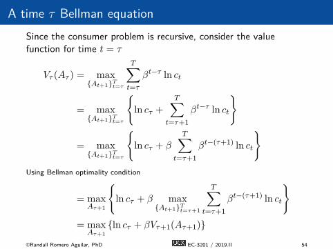
A time τ Bellman equationSince the consumer problem is recursive, consider the valuefunction for time t = τ
Vτ (Aτ ) = max{At+1}Tt=τ
T∑t=τ
βt−τ ln ct
= max{At+1}Tt=τ
{ln cτ +
T∑t=τ+1
βt−τ ln ct
}
= max{At+1}Tt=τ
{ln cτ + β
T∑t=τ+1
βt−(τ+1) ln ct
}Using Bellman optimality condition
= maxAτ+1
{ln cτ + β max
{At+1}Tt=τ+1
T∑t=τ+1
βt−(τ+1) ln ct
}= max
Aτ+1
{ln cτ + βVτ+1(Aτ+1)}
©Randall Romero Aguilar, PhD EC-3201 / 2019.II 54
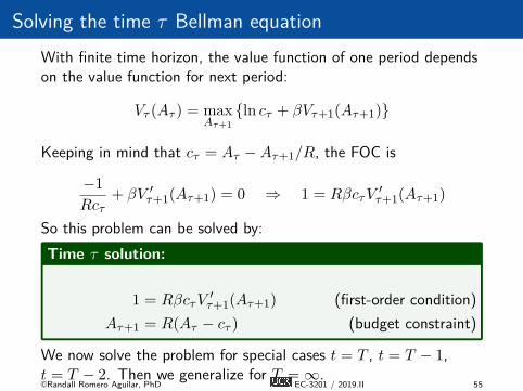
Solving the time τ Bellman equationWith finite time horizon, the value function of one period dependson the value function for next period:
Vτ (Aτ ) = maxAτ+1
{ln cτ + βVτ+1(Aτ+1)}
Keeping in mind that cτ = Aτ −Aτ+1/R, the FOC is
−1
Rcτ+ βV ′
τ+1(Aτ+1) = 0 ⇒ 1 = RβcτV′τ+1(Aτ+1)
So this problem can be solved by:Time τ solution:
1 = RβcτV′τ+1(Aτ+1) (first-order condition)
Aτ+1 = R(Aτ − cτ ) (budget constraint)
We now solve the problem for special cases t = T , t = T − 1,t = T − 2. Then we generalize for T = ∞.©Randall Romero Aguilar, PhD EC-3201 / 2019.II 55

Solution when t = T
In this case, consumer problem is simply
VT (AT ) = maxcT ,AT+1
{ln cT } subject to
AT+1 = R(AT − cT ), AT+1 ≥ 0
We need to find cT and AT+1. Substitute cT = AT − AT+1
R in theobjective function:
maxAT+1
ln[AT − AT+1
R
]subject to AT+1 ≥ 0
This function is strictly decreasing on AT+1, so we set AT+1 toits minimum possible value; given the transversality constraint weset AT+1 = 0, which implies cT = AT and VT (AT ) = lnAT . Inwords, in his last period a consumer spends his entire assets.
©Randall Romero Aguilar, PhD EC-3201 / 2019.II 56

Solution when t = T − 1
The problem is now
VT−1(AT−1) = maxAT
{ln cT−1 + βVT (AT )}
Its solution, since we know that VT (AT ) = lnAT , is given by:{1 = RβcT−1V
′T (AT )
AT = R(AT−1 − cT−1)⇒
{AT = RβcT−1
AT = R(AT−1 − cT−1)
It follows that
c∗T−1 =1
1+βAT−1 ⇒ A∗T = Rβ
1+βAT−1
©Randall Romero Aguilar, PhD EC-3201 / 2019.II 57

The value function is
VT−1(AT−1) = ln c∗T−1 + βVT (A∗T )
= ln c∗T−1 + β lnA∗T
= ln c∗T−1 + β ln[Rβc∗T−1]
= (1 + β) ln c∗T−1 + β lnβ + β lnR
=(1 + β) lnAT−1 − (1 + β) ln(1 + β) + . . .
· · ·+ β lnβ + β lnR
= (1 + β) lnAT−1 + θT−1
where the term θT−1 is just a constant.
©Randall Romero Aguilar, PhD EC-3201 / 2019.II 58

Solution when t = T − 2
The problem is now
VT−2(AT−2) = maxAT−1
{ln cT−2 + βVT−1(AT−1)}
Its solution, since we know thatVT−1(AT−1) = (1 + β) lnAT−1 + θT−1, is given by:
{1 = RβcT−2V
′T−1(AT−1)
AT−1 = R(AT−2 − cT−2)⇒
{AT−1 = Rβ(1 + β)cT−2
AT−1 = R(AT−2 − cT−2)
It follows that
c∗T−2 =1
1+β+β2AT−2 ⇒ A∗T−1 =
R(β+β2)1+β+β2 AT−2
©Randall Romero Aguilar, PhD EC-3201 / 2019.II 59
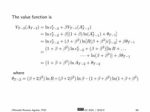
The value function is
VT−2(AT−2) = ln c∗T−2 + βVT−1(A∗T−1)
= ln c∗T−2 + β[(1 + β) ln(A∗T−1) + θT−1]
= ln c∗T−2 + (β + β2) ln[R(β + β2)c∗T−2] + βθT−1
=(1 + β + β2) ln c∗T−2 + (β + β2)[lnR+ . . .
· · ·+ ln(β + β2)] + βθT−1
= (1 + β + β2) lnAT−2 + θT−2
whereθT−2 = (β+2β2) lnR+(β+2β2) lnβ− (1+β+β2) ln(1+β+β2)
©Randall Romero Aguilar, PhD EC-3201 / 2019.II 60

Solution when t = T − k
If we keep iterating, the problem is now
VT−k(AT−k) = maxAT−k+1
{ln cT−k + βVT−k+1(AT−k+1)}
Its solution, is given by:{1 = RβcT−kV
′T−k+1(AT−k+1)
AT−k+1 = R(AT−k − cT−k)
But since we do not know VT−k+1(AT−k+1), we cannot substitutejust yet, unless we solve for all intermediate steps. Instead of doingthat, we will search for patterns in our results.
©Randall Romero Aguilar, PhD EC-3201 / 2019.II 61

Searching for patterns
Let’s summarize the results for the policy function.
t c∗t A∗t+1
T AT 0AT
T −11
1+βAT−1 Rβ 11+βAT−1
T −21
1+β+β2AT−2 Rβ 1+β1+β+β2AT−2
We could guess that after k iterations:
T −k1
1+β+···+βkAT−k Rβ 1+β+···+βk−1
1+β+···+βk AT−k
=1− β
1− βk+1AT−k Rβ
1− βk
1− βk+1AT−k
©Randall Romero Aguilar, PhD EC-3201 / 2019.II 62

The time path of assets
Since AT−k+1 = Rβ 1−βk
1−βk+1AT−k, setting k = T, T − 1:
A1 = Rβ1− βT
1− βT+1A0
A2 = Rβ1− βT−1
1− βTA1
= (Rβ)21− βT−1
1− βT+1A0
Iterating in this fashion we find that
At = (Rβ)t1− βT+1−t
1− βT+1A0
©Randall Romero Aguilar, PhD EC-3201 / 2019.II 63
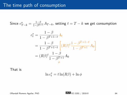
The time path of consumption
Since c∗T−k = 1−β1−βk+1AT−k, setting t = T − k we get consumption
c∗t =1− β
1− βT+1−tAt
=1− β
1− βT+1−t
[(Rβ)t
1− βT+1−t
1− βT+1A0
]= (Rβ)t
1− β
1− βT+1A0
ϕ
That isln c∗t = t ln(Rβ) + lnϕ
©Randall Romero Aguilar, PhD EC-3201 / 2019.II 64

The time 0 value functionSubstitution of the optimal consumption path in the Bellmanequation give the value function
V0(A0) ≡T∑t=0
βt ln c∗t =
T∑t=0
βt (t ln(Rβ) + lnϕ)
= ln(Rβ)T∑t=0
βtt+ lnϕ
T∑t=0
βt
=β
1− β
(1− βT
1− β− TβT
)ln(Rβ) +
1− βT+1
1− βlnϕ
=
β
1− β
(1− βT
1− β− TβT
)ln(Rβ) + . . .
+1− βT+1
1− βln 1− β
1− βT+1+
1− βT+1
1− βlnA0
©Randall Romero Aguilar, PhD EC-3201 / 2019.II 65
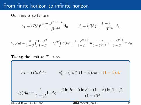
From finite horizon to infinite horizonOur results so far are
At = (Rβ)t1− βT+1−t
1− βT+1A0 c∗t = (Rβ)t
1− β
1− βT+1A0
V0(A0) =β
1− β
(1− βT
1− β− TβT
)ln(Rβ)+
1− βT+1
1− βln 1− β
1− βT+1+1− βT+1
1− βlnA0
Taking the limit as T → ∞
At = (Rβ)tA0 c∗t = (Rβ)t(1− β)A0 = (1− β)At
V0(A0) =1
1− βlnA0 +
β lnR+ β lnβ + (1− β) ln(1− β)
(1− β)2
©Randall Romero Aguilar, PhD EC-3201 / 2019.II 66
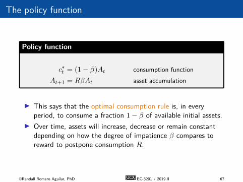
The policy function
Policy function
c∗t = (1− β)At consumption functionAt+1 = RβAt asset accumulation
I This says that the optimal consumption rule is, in everyperiod, to consume a fraction 1− β of available initial assets.
I Over time, assets will increase, decrease or remain constantdepending on how the degree of impatience β compares toreward to postpone consumption R.
©Randall Romero Aguilar, PhD EC-3201 / 2019.II 67
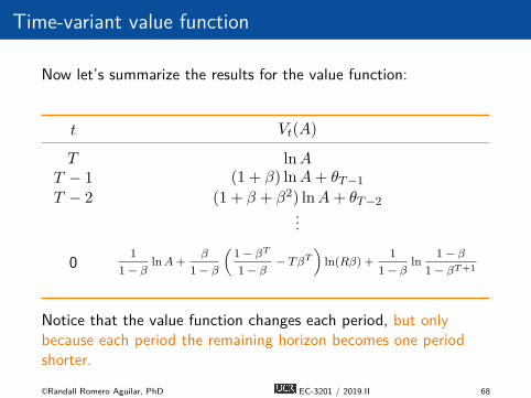
Time-variant value function
Now let’s summarize the results for the value function:
t Vt(A)
T lnAT − 1 (1 + β) lnA+ θT−1
T − 2 (1 + β + β2) lnA+ θT−2...
0 1
1− βlnA+
β
1− β
(1− βT
1− β− TβT
)ln(Rβ) +
1
1− βln 1− β
1− βT+1
Notice that the value function changes each period, but onlybecause each period the remaining horizon becomes one periodshorter.©Randall Romero Aguilar, PhD EC-3201 / 2019.II 68

Time-invariant value function
Remember that in our k iteration,
VT−k(AT−k) = maxcT−k,
AT−k+1
{ln cT−k + βVT−k+1(AT−k+1)}
With an infinite horizon, the remaining horizon is the same inT − k and in T − k+1, so the value function is the same, preciselythe fixed-point of the Bellman equation. Then we can write
V (AT−k) = maxcT−k,
AT−k+1
{ln cT−k + βV (AT−k+1)}
or simplyV (A) = max
c,A′
{ln c+ βV (A′)
}where a prime indicates a next-period variable
©Randall Romero Aguilar, PhD EC-3201 / 2019.II 69

The first order condition
Using the budget constraint to substitute consumption
V (A) = maxA′
{ln
(A− A′
R
)+ βV (A′)
}we obtain the FOC:
1 = RβcV ′(A′)
Despite not knowing V , we can determine its first derivative usingthe envelope condition.Thus, from
V (A) = ln(A− A′∗
R
)+ βV (A′∗)
we getV ′(A) =
1
c
©Randall Romero Aguilar, PhD EC-3201 / 2019.II 70

The Euler condition
I Because the solution is time-invariant, V ′(A) = 1c implies that
V ′(A′) = 1c′ .
I Substitute this into the FOC to obtain theEuler equation
1 = Rβc
c′= Rβ
u′(c′)
u′(c)
I This says that the marginal rate of substitution ofconsumption between any consecutive periods u′(c)
βu′(c′) mustequal the relative price of the later consumption in terms ofthe earlier consumption R.
©Randall Romero Aguilar, PhD EC-3201 / 2019.II 71

Value function iteration
I Suppose we wanted to solve the infinite horizon problem
V (A) = maxc,A′
{ln c+ βV (A′)
}subject to A′ = R(A− c)
by value function iteration:
Vj+1(A) = maxc,A′
{ln c+ βVj(A
′)}
subject to A′ = R(A− c)
I If we start iterating from V0(A) = 0 , our iterations wouldlook identical to the procedure we used to solve for the finitehorizon problem!
©Randall Romero Aguilar, PhD EC-3201 / 2019.II 72

I Then, our iterations would look likej Vj(A)
0 01 lnA2 (1 + β) lnA+ θ23 (1 + β + β2) lnA+ θ3
...I If we keep iterating, we would expect that the coefficient on
lnA would converge to 1 + β + β2 + · · · = 11−β
I However, it is much harder to see a pattern on the θjsequence.
I Then, we could try now the guess and verify, guessing thatthe solution takes the form V (A) = 1
1−β lnA+ θ.
©Randall Romero Aguilar, PhD EC-3201 / 2019.II 73

Guess and verify
I Our guess: V (A) = 11−β lnA+ θ
I Solution must satisfy the FOC: 1 = RβcV ′(A′) and budgetconstraint A′ = R(A− c).
I Combining these conditions we find c∗ = (1− β)A andA′∗ = RβA.
I To be a solution of the Bellman equation, it must be the casethat both sides are equal:
©Randall Romero Aguilar, PhD EC-3201 / 2019.II 74
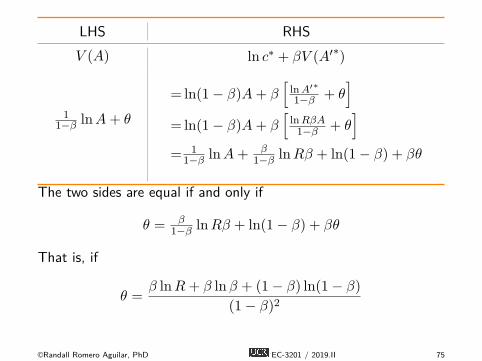
LHS RHSV (A) ln c∗ + βV (A′∗)
11−β lnA+ θ
= ln(1− β)A+ β[
lnA′∗
1−β + θ]
= ln(1− β)A+ β[
lnRβA1−β + θ
]= 1
1−β lnA+ β1−β lnRβ + ln(1− β) + βθ
The two sides are equal if and only if
θ = β1−β lnRβ + ln(1− β) + βθ
That is, if
θ =β lnR+ β lnβ + (1− β) ln(1− β)
(1− β)2
©Randall Romero Aguilar, PhD EC-3201 / 2019.II 75

Why the envelope condition works?
The last point in our discussion is to justify the envelope condition:deriving V (A) pretending that A′∗ did not depend on A. But weknow it does, so write A′∗ = h(A) for some function h. From thedefinition of the value function write:
V (A) = ln[A− h(A)
R
]+ βV (h(A))
Take derivative and arrange terms:
V ′(A) =1
c
[1− h′(A)
R
]+ βV ′(h(A))h′(A)
=1
c+
[−1
cR+ βV ′(A′∗)
]h′(A)
but the term in square brackets must be zero from the FOC.
©Randall Romero Aguilar, PhD EC-3201 / 2019.II 76

5. Consumption and physical investment

A model with production
In this modelI the consumer is endowed with k0 units of a good that can be
used either for consumption or for the production of additionalgood
I we refer to “capital” to the part of the good that is used forfuture production
I capital fully depreciates with the production process.I The lifetime utility of the consumer is again
U(c0, c1, . . . , c∞) =∑∞
t=0 βt ln ct,
I The production function is y = Akα, where A > 0 and0 < α < 1 are parameters.
I The budget constraint is ct + kt+1 = Akαt .
©Randall Romero Aguilar, PhD EC-3201 / 2019.II 77
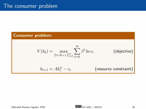
The consumer problem
Consumer problem:
V (k0) = max{ct,kt+1}∞t=0
∞∑t=0
βt ln ct (objective)
kt+1 = Akαt − ct (resource constraint)
©Randall Romero Aguilar, PhD EC-3201 / 2019.II 78
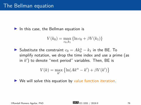
The Bellman equation
I In this case, the Bellman equation is
V (k0) = maxc0,k1
{ln c0 + βV (k1)}
I Substitute the constraint c0 = Akα0 − k1 in the BE. Tosimplify notation, we drop the time index and use a prime (asin k′) to denote “next period” variables. Then, BE is
V (k) = maxk′
{ln(Akα − k′) + βV (k′)
}I We will solve this equation by value function iteration.
©Randall Romero Aguilar, PhD EC-3201 / 2019.II 79
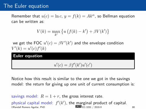
The Euler equationRemember that u(c) = ln c, y = f(k) = Akα, so Bellman equationcan be written as:
V (k) = maxk′
{u(f(k)− k′
)+ βV (k′)
}we get the FOC u′(c) = βV ′(k′) and the envelope conditionV ′(k) = u′(c)f ′(k)
Euler equation
u′(c) = βf ′(k′)u′(c′)
Notice how this result is similar to the one we got in the savingsmodel: the return for giving up one unit of current consumption is:
savings model: R = 1 + r, the gross interest rate.physical capital model: f ′(k′), the marginal product of capital.©Randall Romero Aguilar, PhD EC-3201 / 2019.II 80

Solving Bellman equation by function iteration
I How do we solve the Bellman equation?
V (k) = maxk′
{ln(Akα − k′) + βV (k′)
}I This equation involves a functional, where the unknown is the
function V (k).I Unfortunately, we cannot solve for V directly.I However, this equation is a contraction mapping (as long as
|β| < 1) that has a fixed point (its solution).I Let’s pick an initial guess (V0(k) = 0 is a convenient one) and
them iterate over the Bellman equation by*
Vj+1(k) = maxk′
{ln(Akα − k′) + βVj(k
′)}
*The j subscript refers to an iteration, not to the horizon.©Randall Romero Aguilar, PhD EC-3201 / 2019.II 81

Starting from V0 = 0, the problem becomes:
V1(k) = maxk′
{ln(Akα − k′) + β × 0
}Since the objective is decreasing on k′ and we have the restrictionk′ ≥ 0, the solution is simply k′∗ = 0. Then c∗ = Akα
V1(k) = ln c∗ + β × 0
= ln (Akα)
= lnA+ α ln k
This completes our first iteration. Let’s now find V2:
V2(k) = maxk′
{ln(Akα − k′) + β[lnA+ α ln k′]
}
©Randall Romero Aguilar, PhD EC-3201 / 2019.II 82

FOC is1
Akα − k′=
αβ
k′⇒ k′∗ =
αβ
1 + αβAkα = θ1Ak
α
Then consumption is c∗ = (1− θ1)Akα = 1
1+αβAkα and
V2(k) = ln(c∗) + β lnA+ αβ ln k′∗
= ln(1− θ1) + ln(Akα) + β[lnA+ α ln θ1 + α ln(Akα)]= (1 + αβ) ln(Akα) + β lnA+ [ln(1− θ1) + αβ ln θ1]
= (1 + αβ) ln(Akα) + ϕ2
This completes the second iteration.
©Randall Romero Aguilar, PhD EC-3201 / 2019.II 83

Let’s have one more:
V3(k) = maxk′
{ln(Akα − k′) + β[(1 + αβ) ln(Ak′α) + ϕ2]
}The FOC is
1
Akα − k′=
αβ(1 + αβ)
k′
k′∗ =αβ + α2β2
1 + αβ + α2β2Akα = θ2Ak
α
Then consumption is c∗ = (1− θ2)Akα = 1
1+αβ+α2β2Akα
After substitution of c∗ and k′∗ into the Bellman equation (and alot of cumbersome algebra):
V3(k) = ln(c∗) + β[(1 + αβ) ln(Ak′∗α) + ϕ2]
= (1 + αβ + α2β2) ln(Akα) + ϕ3
This completes the third iteration.©Randall Romero Aguilar, PhD EC-3201 / 2019.II 84

Searching for patterns
You might be tired by now of iterating this function. Me too! Solet’s try to find some patterns (unless you really want to iterate toinfinity). Let’s summarize the results for the value function.
j V (k)
1 (1) ln (Akα)2 (1 + αβ) ln (Akα) + ϕ2
3 (1 + αβ + α2β2) ln (Akα) + ϕ3
From this table, we could guess that after j iterations, theconsumption policy would look like:
Vj(k) = (1 + αβ + . . .+ αjβj) ln (Akα) + ϕj
©Randall Romero Aguilar, PhD EC-3201 / 2019.II 85

Iterating to infinity
I To converge to the fixed point, we need to iterate to infinity.I Simply take the limit j → ∞ of the value function: since
0 < αβ < 1, the geometric series converges, and so
V (k) = 11−αβ ln (Akα) + Φ
I Notice that we did not formally prove that the ϕj sequenceactually converges (so far we are just assuming it does.)
©Randall Romero Aguilar, PhD EC-3201 / 2019.II 86
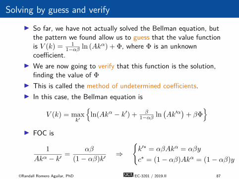
Solving by guess and verifyI So far, we have not actually solved the Bellman equation, but
the pattern we found allow us to guess that the value functionis V (k) = 1
1−αβ ln (Akα) + Φ, where Φ is an unknowncoefficient.
I We are now going to verify that this function is the solution,finding the value of Φ
I This is called the method of undetermined coefficients.I In this case, the Bellman equation is
V (k) = maxk′
{ln(Akα − k′) + β
1−αβ ln(Ak′α
)+ βΦ
}I FOC is
1
Akα − k′=
αβ
(1− αβ)k′⇒
{k′∗ = αβAkα = αβy
c∗ = (1− αβ)Akα = (1− αβ)y
©Randall Romero Aguilar, PhD EC-3201 / 2019.II 87
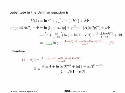
Substitute in the Bellman equation is
V (k) = ln c∗ + β1−αβ ln
(Ak′α
)+ βΦ
11−αβ ln(Akα) + Φ = ln [(1− αβ)y] + β
1−αβ ln [A (αβy)α] + βΦ
=(1 + αβ
1−αβ
)ln y + ln(1− αβ) + β ln[A(αβ)α]
1−αβ + βΦ
= 11−αβ ln y + (1−αβ) ln(1−αβ)+β ln[A(αβ)α]
1−αβ + βΦ
Therefore
(1− β)Φ= (1−αβ) ln(1−αβ)+β ln[A(αβ)α]1−αβ
Φ =β lnA+ ln (αβ)αβ + ln(1− αβ)(1−αβ)
(1− β)(1− αβ)
©Randall Romero Aguilar, PhD EC-3201 / 2019.II 88

Finally, the policy and value functions are given by
k′∗(k) = αβAkα
c∗(k) = (1− αβ)Akα
V (k) =1
1− αβln (Akα) + β lnA+ln(αβ)αβ+ln(1−αβ)(1−αβ)
(1−β)(1−αβ)
©Randall Romero Aguilar, PhD EC-3201 / 2019.II 89
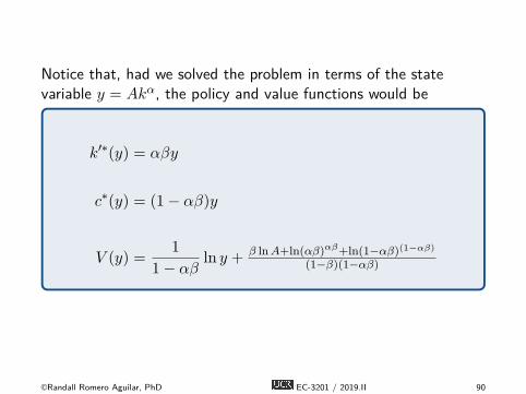
Notice that, had we solved the problem in terms of the statevariable y = Akα, the policy and value functions would be
k′∗(y) = αβy
c∗(y) = (1− αβ)y
V (y) =1
1− αβln y + β lnA+ln(αβ)αβ+ln(1−αβ)(1−αβ)
(1−β)(1−αβ)
©Randall Romero Aguilar, PhD EC-3201 / 2019.II 90

6. The McCall job search model
Overview
I The McCall search model :cite:‘McCall1970‘ helped transformeconomists’ way of thinking about labor markets.
I To clarify vague notions such as ”involuntary” unemployment,McCall modeled the decision problem of unemployed agentsdirectly, in terms of factors such asI current and likely future wagesI impatienceI unemployment compensation
I To solve the decision problem he used dynamic programming.I Here we set up McCall’s model and adopt the same solution
method.I As we’ll see, McCall’s model is not only interesting in its own
right but also an excellent vehicle for learning dynamicprogramming.
©Randall Romero Aguilar, PhD EC-3201 / 2019.II 91
The McCall Model
I An unemployed worker receives in each period a job offer atwage Wt.
I At time t, our worker has two choices:1. Accept the offer and work permanently at constant wage Wt.2. Reject the offer, receive unemployment compensation c, and
reconsider next period.I The wage sequence is assumed to be IID with probability
mass function ϕ.I Thus ϕ(w) is the probability of observing wage offer w in the
set {w1, . . . , wn}.
©Randall Romero Aguilar, PhD EC-3201 / 2019.II 92
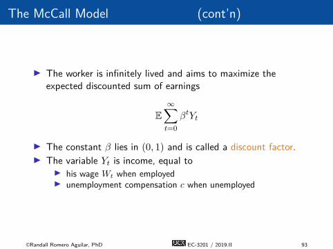
The McCall Model (cont’n)
I The worker is infinitely lived and aims to maximize theexpected discounted sum of earnings
E∞∑t=0
βtYt
I The constant β lies in (0, 1) and is called a discount factor.I The variable Yt is income, equal to
I his wage Wt when employedI unemployment compensation c when unemployed
©Randall Romero Aguilar, PhD EC-3201 / 2019.II 93

A Trade-Off
I The worker faces a trade-off:I Waiting too long for a good offer is costly, since the future is
discounted.I Accepting too early is costly, since better offers might arrive in
the future.I To decide optimally in the face of this trade-off, we use
dynamic programming.I Dynamic programming can be thought of as a two-step
procedure that1. first assigns values to ”states” and2. then deduces optimal actions given those values
I We’ll go through these steps in turn.
©Randall Romero Aguilar, PhD EC-3201 / 2019.II 94
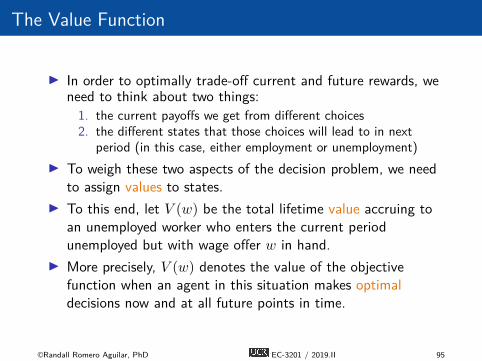
The Value Function
I In order to optimally trade-off current and future rewards, weneed to think about two things:
1. the current payoffs we get from different choices2. the different states that those choices will lead to in next
period (in this case, either employment or unemployment)I To weigh these two aspects of the decision problem, we need
to assign values to states.I To this end, let V (w) be the total lifetime value accruing to
an unemployed worker who enters the current periodunemployed but with wage offer w in hand.
I More precisely, V (w) denotes the value of the objectivefunction when an agent in this situation makes optimaldecisions now and at all future points in time.
©Randall Romero Aguilar, PhD EC-3201 / 2019.II 95

The Value Function (cont’n)
I Of course V (w) is not trivial to calculate because we don’tyet know what decisions are optimal and what aren’t!
I But think of V as a function that assigns to each possiblewage w the maximal lifetime value that can be obtained withthat offer in hand.
I A crucial observation is that this function V must satisfy therecursion
V (w) = max{
w
1− β, c+ β
∑w′
V (w′)ϕ(w′)
}
for every possible w in {w1, . . . , wn}.I This important equation is a version of the Bellman equation,
which is ubiquitous in economic dynamics and other fieldsinvolving planning over time.
©Randall Romero Aguilar, PhD EC-3201 / 2019.II 96

The Value Function (cont’n)
V (w) = max{
w
1− β, c+ β
∑w′
V (w′)ϕ(w′)
}
I The intuition behind it is as follows:1. the first term inside the max operation is the lifetime payoff
from accepting current offer w, since
w + βw + β2w + · · · = w
1− β
2. the second term inside the max operation is the continuationvalue, which is the lifetime payoff from rejecting the currentoffer and then behaving optimally in all subsequent periods
I If we optimize and pick the best of these two options, weobtain maximal lifetime value from today, given current offerw.
I But this is precisely V (w), which is the l.h.s. of the Bellmanequation.
©Randall Romero Aguilar, PhD EC-3201 / 2019.II 97

The Optimal Policy
I Suppose for now that we are able to solve the Bellmanequation for the unknown function V .
I Once we have this function in hand we can behave optimally(i.e., make the right choice between accept and reject).
I All we have to do is select the maximal choice on the r.h.s. ofthe Bellman equation.
I The optimal action is best thought of as a policy, which is, ingeneral, a map from states to actions.
I In our case, the state is the current wage offer w.
©Randall Romero Aguilar, PhD EC-3201 / 2019.II 98
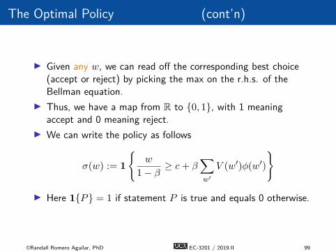
The Optimal Policy (cont’n)
I Given any w, we can read off the corresponding best choice(accept or reject) by picking the max on the r.h.s. of theBellman equation.
I Thus, we have a map from R to {0, 1}, with 1 meaningaccept and 0 meaning reject.
I We can write the policy as follows
σ(w) := 1{
w
1− β≥ c+ β
∑w′
V (w′)ϕ(w′)
}
I Here 1{P} = 1 if statement P is true and equals 0 otherwise.
©Randall Romero Aguilar, PhD EC-3201 / 2019.II 99

The Reservation Wage
I We can also write the policy function as
σ(w) := 1{w ≥ w̄}
where
w̄ := (1− β)
{c+ β
∑w′
V (w′)ϕ(w′)
}I Here w̄ is a constant depending on β, c and the wage
distribution called the reservation wage.I The agent should accept if and only if the current wage offer
exceeds the reservation wage.I Clearly, we can compute this reservation wage if we can
compute the value function.
©Randall Romero Aguilar, PhD EC-3201 / 2019.II 100

Computing the Optimal Policy
I Solving this model requires numerical methods, which arebeyond the scope of this course.
I Those interested in this topic should take a look athttps://python.quantecon.org/mccall_model.html
I Indeed, the notes on this section on the McCall search modelwhere taken from this website, which is part of thehttps://quantecon.org/ website by Sargent andStachurski.
©Randall Romero Aguilar, PhD EC-3201 / 2019.II 101

References I
Chiang, Alpha C. (1992). Elements of Dynamic Optimization.McGraw-Hill, Inc.
Ljungqvist, Lars and Thomas J. Sargent (2004). RecursiveMacroeconomic Theory. 2nd ed. MIT Press. isbn: 0-262-12274-X.
Miranda, Mario J. and Paul L. Fackler (2002). Applied ComputationalEconomics and Finance. MIT Press. isbn: 0-262-13420-9.
Romero-Aguilar, Randall (2016). CompEcon-Python. url:http://randall-romero.com/code/compecon/.
Sargent, Thomas J. and John Stachurski (2016). QuantitativeEconomics. url: http://lectures.quantecon.org/.
©Randall Romero Aguilar, PhD EC-3201 / 2019.II 102