Earth’s energy imbalance and implications
29
Atmos. Chem. Phys., 11, 13421–13449, 2011 www.atmos-chem-phys.net/11/13421/2011/ doi:10.5194/acp-11-13421-2011 © Author(s) 2011. CC Attribution 3.0 License. Atmospheric Chemistry and Physics Earth’s energy imbalance and implications J. Hansen 1,2 , M. Sato 1,2 , P. Kharecha 1,2 , and K. von Schuckmann 3 1 NASA Goddard Institute for Space Studies, New York, NY 10025, USA 2 Columbia University Earth Institute, New York, NY 10027, USA 3 Centre National de la Recherche Scientifique, LOCEAN Paris, hosted by Ifremer, Brest, France Received: 2 September 2011 – Published in Atmos. Chem. Phys. Discuss.: 29 September 2011 Revised: 30 November 2011 – Accepted: 7 December 2011 – Published: 22 December 2011 Abstract. Improving observations of ocean heat content show that Earth is absorbing more energy from the Sun than it is radiating to space as heat, even during the recent solar minimum. The inferred planetary energy imbalance, 0.58 ± 0.15 W m -2 during the 6-yr period 2005–2010, con- firms the dominant role of the human-made greenhouse ef- fect in driving global climate change. Observed surface tem- perature change and ocean heat gain together constrain the net climate forcing and ocean mixing rates. We conclude that most climate models mix heat too efficiently into the deep ocean and as a result underestimate the negative forcing by human-made aerosols. Aerosol climate forcing today is in- ferred to be -1.6 ± 0.3 W m -2 , implying substantial aerosol indirect climate forcing via cloud changes. Continued failure to quantify the specific origins of this large forcing is unten- able, as knowledge of changing aerosol effects is needed to understand future climate change. We conclude that recent slowdown of ocean heat uptake was caused by a delayed re- bound effect from Mount Pinatubo aerosols and a deep pro- longed solar minimum. Observed sea level rise during the Argo float era is readily accounted for by ice melt and ocean thermal expansion, but the ascendency of ice melt leads us to anticipate acceleration of the rate of sea level rise this decade. 1 Introduction Humanity is potentially vulnerable to global temperature change, as discussed in the Intergovernmental Panel on Climate Change (IPCC, 2001, 2007) reports and by innu- merable authors. Although climate change is driven by many climate forcing agents and the climate system also ex- hibits unforced (chaotic) variability, it is now widely agreed that the strong global warming trend of recent decades is Correspondence to: J. Hansen ([email protected]) caused predominantly by human-made changes of atmo- spheric composition (IPCC, 2007). The basic physics underlying this global warming, the greenhouse effect, is simple. An increase of gases such as CO 2 makes the atmosphere more opaque at infrared wave- lengths. This added opacity causes the planet’s heat radiation to space to arise from higher, colder levels in the atmosphere, thus reducing emission of heat energy to space. The tempo- rary imbalance between the energy absorbed from the Sun and heat emission to space, causes the planet to warm until planetary energy balance is restored. The planetary energy imbalance caused by a change of at- mospheric composition defines a climate forcing. Climate sensitivity, the eventual global temperature change per unit forcing, is known with good accuracy from Earth’s paleocli- mate history. However, two fundamental uncertainties limit our ability to predict global temperature change on decadal time scales. First, although climate forcing by human-made green- house gases (GHGs) is known accurately, climate forcing caused by changing human-made aerosols is practically un- measured. Aerosols are fine particles suspended in the air, such as dust, sulfates, and black soot (Ramanathan et al., 2001). Aerosol climate forcing is complex, because aerosols both reflect solar radiation to space (a cooling effect) and absorb solar radiation (a warming effect). In addition, at- mospheric aerosols can alter cloud cover and cloud proper- ties. Therefore, precise composition-specific measurements of aerosols and their effects on clouds are needed to assess the aerosol role in climate change. Second, the rate at which Earth’s surface temperature ap- proaches a new equilibrium in response to a climate forcing depends on how efficiently heat perturbations are mixed into the deeper ocean. Ocean mixing is complex and not neces- sarily simulated well by climate models. Empirical data on ocean heat uptake are improving rapidly, but still suffer lim- itations. Published by Copernicus Publications on behalf of the European Geosciences Union.
Transcript of Earth’s energy imbalance and implications

Atmos. Chem. Phys., 11, 13421–13449, 2011www.atmos-chem-phys.net/11/13421/2011/doi:10.5194/acp-11-13421-2011© Author(s) 2011. CC Attribution 3.0 License.
AtmosphericChemistry
and Physics
Earth’s energy imbalance and implications
J. Hansen1,2, M. Sato1,2, P. Kharecha1,2, and K. von Schuckmann3
1NASA Goddard Institute for Space Studies, New York, NY 10025, USA2Columbia University Earth Institute, New York, NY 10027, USA3Centre National de la Recherche Scientifique, LOCEAN Paris, hosted by Ifremer, Brest, France
Received: 2 September 2011 – Published in Atmos. Chem. Phys. Discuss.: 29 September 2011Revised: 30 November 2011 – Accepted: 7 December 2011 – Published: 22 December 2011
Abstract. Improving observations of ocean heat contentshow that Earth is absorbing more energy from the Sunthan it is radiating to space as heat, even during the recentsolar minimum. The inferred planetary energy imbalance,0.58± 0.15 W m−2 during the 6-yr period 2005–2010, con-firms the dominant role of the human-made greenhouse ef-fect in driving global climate change. Observed surface tem-perature change and ocean heat gain together constrain thenet climate forcing and ocean mixing rates. We conclude thatmost climate models mix heat too efficiently into the deepocean and as a result underestimate the negative forcing byhuman-made aerosols. Aerosol climate forcing today is in-ferred to be−1.6± 0.3 W m−2, implying substantial aerosolindirect climate forcing via cloud changes. Continued failureto quantify the specific origins of this large forcing is unten-able, as knowledge of changing aerosol effects is needed tounderstand future climate change. We conclude that recentslowdown of ocean heat uptake was caused by a delayed re-bound effect from Mount Pinatubo aerosols and a deep pro-longed solar minimum. Observed sea level rise during theArgo float era is readily accounted for by ice melt and oceanthermal expansion, but the ascendency of ice melt leads us toanticipate acceleration of the rate of sea level rise this decade.
1 Introduction
Humanity is potentially vulnerable to global temperaturechange, as discussed in the Intergovernmental Panel onClimate Change (IPCC, 2001, 2007) reports and by innu-merable authors. Although climate change is driven bymany climate forcing agents and the climate system also ex-hibits unforced (chaotic) variability, it is now widely agreedthat the strong global warming trend of recent decades is
Correspondence to:J. Hansen([email protected])
caused predominantly by human-made changes of atmo-spheric composition (IPCC, 2007).
The basic physics underlying this global warming, thegreenhouse effect, is simple. An increase of gases such asCO2 makes the atmosphere more opaque at infrared wave-lengths. This added opacity causes the planet’s heat radiationto space to arise from higher, colder levels in the atmosphere,thus reducing emission of heat energy to space. The tempo-rary imbalance between the energy absorbed from the Sunand heat emission to space, causes the planet to warm untilplanetary energy balance is restored.
The planetary energy imbalance caused by a change of at-mospheric composition defines a climate forcing. Climatesensitivity, the eventual global temperature change per unitforcing, is known with good accuracy from Earth’s paleocli-mate history. However, two fundamental uncertainties limitour ability to predict global temperature change on decadaltime scales.
First, although climate forcing by human-made green-house gases (GHGs) is known accurately, climate forcingcaused by changing human-made aerosols is practically un-measured. Aerosols are fine particles suspended in the air,such as dust, sulfates, and black soot (Ramanathan et al.,2001). Aerosol climate forcing is complex, because aerosolsboth reflect solar radiation to space (a cooling effect) andabsorb solar radiation (a warming effect). In addition, at-mospheric aerosols can alter cloud cover and cloud proper-ties. Therefore, precise composition-specific measurementsof aerosols and their effects on clouds are needed to assessthe aerosol role in climate change.
Second, the rate at which Earth’s surface temperature ap-proaches a new equilibrium in response to a climate forcingdepends on how efficiently heat perturbations are mixed intothe deeper ocean. Ocean mixing is complex and not neces-sarily simulated well by climate models. Empirical data onocean heat uptake are improving rapidly, but still suffer lim-itations.
Published by Copernicus Publications on behalf of the European Geosciences Union.

13422 J. Hansen et al.: Earth’s energy imbalance and implications
Fig. 1. Climate forcings employed in this paper. Forcings through 2003 (vertical line) are the same as used by Hansen et al. (2007), except the tropospheric aerosol forcing after 1990 is approximated as -0.5 times the GHG forcing. Aerosol forcing includes all aerosol effects, including indirect effects on clouds and snow albedo. GHGs include O3 and stratospheric H2O, in addition to well-mixed GHGs.These data are available at http://www.columbia.edu/~mhs119/EnergyImbalance/Imbalance.Fig01.txt
1
Fig. 1. Climate forcings employed in this paper. Forcings through 2003 (vertical line) are the same as used by Hansen et al. (2007), exceptthe tropospheric aerosol forcing after 1990 is approximated as−0.5 times the GHG forcing. Aerosol forcing includes all aerosol effects,including indirect effects on clouds and snow albedo. GHGs include O3 and stratospheric H2O, in addition to well-mixed GHGs. These dataare available athttp://www.columbia.edu/∼mhs119/EnergyImbalance/Imbalance.Fig01.txt.
We summarize current understanding of this basic physicsof global warming and note observations needed to narrowuncertainties. Appropriate measurements can quantify themajor factors driving climate change, reveal how much ad-ditional global warming is already in the pipeline, and helpdefine the reduction of climate forcing needed to stabilizeclimate.
2 Climate forcings
A climate forcing is an imposed perturbation of Earth’s en-ergy balance. Natural forcings include changes of solar ir-radiance and volcanic eruptions that inject aerosols to al-titudes 10–30 km in the stratosphere, where they reside 1–2 yr, reflecting sunlight and cooling Earth’s surface. Principalhuman-made forcings are greenhouse gases and troposphericaerosols, i.e., aerosols in Earth’s lower atmosphere, mostly inthe lowest few kilometers of the atmosphere. Human-madechanges of land use and land cover are important regionally,but are much less important than atmospheric compositionover the past century (Ramankutty and Foley, 1999; Hansenet al., 2007).
A forcing, F , is measured in watts per square meter(W m−2) averaged over the planet. For example, if the Sun’sbrightness increases 1 percent the forcing isF ∼ 2.4 W m−2,because Earth absorbs about 240 W m−2 of solar energy av-eraged over the planet’s surface. If the CO2 amount in the airis doubled1, the forcing isF ∼ 4 W m−2. The opacity of agreenhouse gas as a function of wavelength is calculated via
1 CO2 climate forcing is approximately logarithmic, because itsabsorption bands saturate as CO2 amount increases. An equationfor climate forcing as a function of CO2 amount is given in Table 1of Hansen et al. (2000).
basic quantum physics and verified by laboratory measure-ments to an accuracy of a few percent. No climate model isneeded to calculate the forcing due to changed greenhousegas amount. It requires only summing over the planet thechange of heat radiation to space, which depends on knownatmospheric and surface properties.
We employ climate forcings (Fig. 1) described elsewhere(Hansen et al., 2007) for simplified calculations of globaltemperature, demonstrating that a simple Green’s functioncalculation, with negligible computation time, yields prac-tically the same global temperature change as the complexclimate model, provided that the global model’s “climate re-sponse function” has been defined. The response functionspecifies the fraction of the equilibrium (long-term) responseachieved as a function of time following imposition of theforcing The simplified calculations allow investigation of theconsequences of errors in aerosol climate forcing and oceanheat uptake.
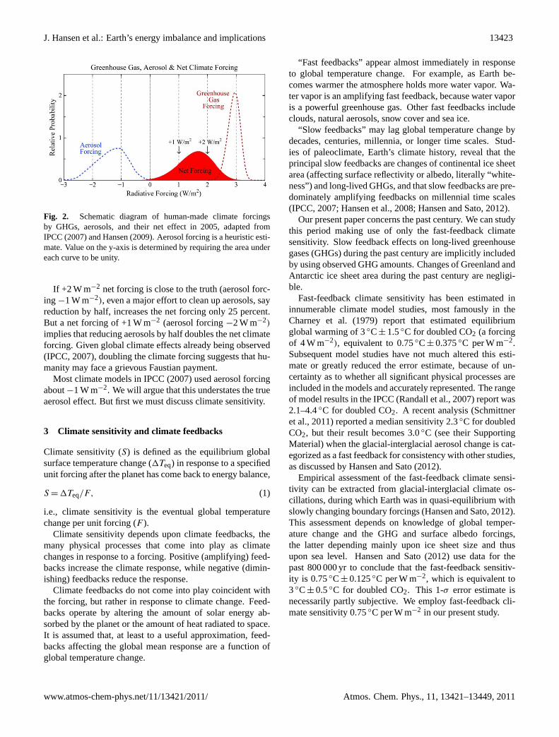
The importance of the uncertainty in aerosol forcing ishighlighted by considering two specific values of the net(GHG + aerosol) forcing: +1 W m−2 and +2 W m−2 (Fig. 2).Either of these values has a good chance of being correct,because the aerosol forcing is unmeasured. Which of thesevalues is closer to the truth defines the terms of humanity’s“Faustian aerosol bargain” (Hansen and Lacis, 1990). Globalwarming so far has been limited, because aerosol coolingpartially offsets GHG warming. But aerosols remain air-borne only several days, so they must be pumped into theair faster and faster to keep pace with increasing long-livedGHGs. However, concern about health effects of particulateair pollution is likely to lead to eventual reduction of human-made aerosols. Thereupon the Faustian payment will comedue.
Atmos. Chem. Phys., 11, 13421–13449, 2011 www.atmos-chem-phys.net/11/13421/2011/
J. Hansen et al.: Earth’s energy imbalance and implications 13423
Fig. 1. Climate forcings employed in this paper. Forcings through 2003 (vertical line) are the same as used by Hansen et al. (2007), except the tropospheric aerosol forcing after 1990 is approximated as -0.5 times the GHG forcing. Aerosol forcing includes all aerosol effects, including indirect effects on clouds and snow albedo. GHGs include O3 and stratospheric H2O, in addition to well-mixed GHGs.These data are available at http://www.columbia.edu/~mhs119/EnergyImbalance/Imbalance.Fig01.txt
1
Fig. 2. Schematic diagram of human-made climate forcingsby GHGs, aerosols, and their net effect in 2005, adapted fromIPCC (2007) and Hansen (2009). Aerosol forcing is a heuristic esti-mate. Value on the y-axis is determined by requiring the area undereach curve to be unity.
If +2 W m−2 net forcing is close to the truth (aerosol forc-ing −1 W m−2), even a major effort to clean up aerosols, sayreduction by half, increases the net forcing only 25 percent.But a net forcing of +1 W m−2 (aerosol forcing−2 W m−2)
implies that reducing aerosols by half doubles the net climateforcing. Given global climate effects already being observed(IPCC, 2007), doubling the climate forcing suggests that hu-manity may face a grievous Faustian payment.
Most climate models in IPCC (2007) used aerosol forcingabout−1 W m−2. We will argue that this understates the trueaerosol effect. But first we must discuss climate sensitivity.
3 Climate sensitivity and climate feedbacks
Climate sensitivity (S) is defined as the equilibrium globalsurface temperature change (1Teq) in response to a specifiedunit forcing after the planet has come back to energy balance,
S = 1Teq/F, (1)
i.e., climate sensitivity is the eventual global temperaturechange per unit forcing (F ).
Climate sensitivity depends upon climate feedbacks, themany physical processes that come into play as climatechanges in response to a forcing. Positive (amplifying) feed-backs increase the climate response, while negative (dimin-ishing) feedbacks reduce the response.
Climate feedbacks do not come into play coincident withthe forcing, but rather in response to climate change. Feed-backs operate by altering the amount of solar energy ab-sorbed by the planet or the amount of heat radiated to space.It is assumed that, at least to a useful approximation, feed-backs affecting the global mean response are a function ofglobal temperature change.
“Fast feedbacks” appear almost immediately in responseto global temperature change. For example, as Earth be-comes warmer the atmosphere holds more water vapor. Wa-ter vapor is an amplifying fast feedback, because water vaporis a powerful greenhouse gas. Other fast feedbacks includeclouds, natural aerosols, snow cover and sea ice.
“Slow feedbacks” may lag global temperature change bydecades, centuries, millennia, or longer time scales. Stud-ies of paleoclimate, Earth’s climate history, reveal that theprincipal slow feedbacks are changes of continental ice sheetarea (affecting surface reflectivity or albedo, literally “white-ness”) and long-lived GHGs, and that slow feedbacks are pre-dominately amplifying feedbacks on millennial time scales(IPCC, 2007; Hansen et al., 2008; Hansen and Sato, 2012).
Our present paper concerns the past century. We can studythis period making use of only the fast-feedback climatesensitivity. Slow feedback effects on long-lived greenhousegases (GHGs) during the past century are implicitly includedby using observed GHG amounts. Changes of Greenland andAntarctic ice sheet area during the past century are negligi-ble.
Fast-feedback climate sensitivity has been estimated ininnumerable climate model studies, most famously in theCharney et al. (1979) report that estimated equilibriumglobal warming of 3◦C± 1.5◦C for doubled CO2 (a forcingof 4 W m−2), equivalent to 0.75◦C± 0.375◦C per W m−2.Subsequent model studies have not much altered this esti-mate or greatly reduced the error estimate, because of un-certainty as to whether all significant physical processes areincluded in the models and accurately represented. The rangeof model results in the IPCC (Randall et al., 2007) report was2.1–4.4◦C for doubled CO2. A recent analysis (Schmittneret al., 2011) reported a median sensitivity 2.3◦C for doubledCO2, but their result becomes 3.0◦C (see their SupportingMaterial) when the glacial-interglacial aerosol change is cat-egorized as a fast feedback for consistency with other studies,as discussed by Hansen and Sato (2012).
Empirical assessment of the fast-feedback climate sensi-tivity can be extracted from glacial-interglacial climate os-cillations, during which Earth was in quasi-equilibrium withslowly changing boundary forcings (Hansen and Sato, 2012).This assessment depends on knowledge of global temper-ature change and the GHG and surface albedo forcings,the latter depending mainly upon ice sheet size and thusupon sea level. Hansen and Sato (2012) use data for thepast 800 000 yr to conclude that the fast-feedback sensitiv-ity is 0.75◦C± 0.125◦C per W m−2, which is equivalent to3◦C± 0.5◦C for doubled CO2. This 1-σ error estimate isnecessarily partly subjective. We employ fast-feedback cli-mate sensitivity 0.75◦C per W m−2 in our present study.
www.atmos-chem-phys.net/11/13421/2011/ Atmos. Chem. Phys., 11, 13421–13449, 2011
13424 J. Hansen et al.: Earth’s energy imbalance and implications
4 Climate response function
Climate response to human and natural forcings can be sim-ulated with complex global climate models, and, using suchmodels, it has been shown that warming of the ocean in re-cent decades can be reproduced well (Barnett et al., 2005;Hansen et al., 2005; Pierce et al., 2006). Here we seek a sim-ple general framework to examine and compare models andthe real world in terms of fundamental quantities that eluci-date the significance of the planet’s energy imbalance.
Global surface temperature does not respond quickly to aclimate forcing, the response being slowed by the thermalinertia of the climate system. The ocean provides most ofthe heat storage capacity, because approximately its upper100 m is rapidly mixed by wind stress and convection (mix-ing is deepest in winter at high latitudes, where mixing occa-sionally extends into the deep ocean). Thermal inertia of theocean mixed layer, by itself, would lead to a surface temper-ature response time of about a decade, but exchange of waterbetween the mixed layer and deeper ocean increases the sur-face temperature response time by an amount that dependson the rate of mixing and climate sensitivity (Hansen et al.,1985).
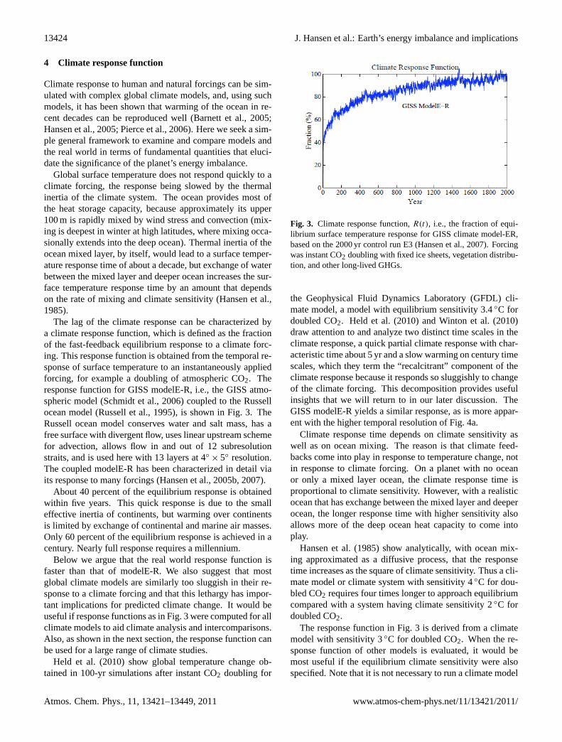
The lag of the climate response can be characterized bya climate response function, which is defined as the fractionof the fast-feedback equilibrium response to a climate forc-ing. This response function is obtained from the temporal re-sponse of surface temperature to an instantaneously appliedforcing, for example a doubling of atmospheric CO2. Theresponse function for GISS modelE-R, i.e., the GISS atmo-spheric model (Schmidt et al., 2006) coupled to the Russellocean model (Russell et al., 1995), is shown in Fig. 3. TheRussell ocean model conserves water and salt mass, has afree surface with divergent flow, uses linear upstream schemefor advection, allows flow in and out of 12 subresolutionstraits, and is used here with 13 layers at 4◦
× 5◦ resolution.The coupled modelE-R has been characterized in detail viaits response to many forcings (Hansen et al., 2005b, 2007).
About 40 percent of the equilibrium response is obtainedwithin five years. This quick response is due to the smalleffective inertia of continents, but warming over continentsis limited by exchange of continental and marine air masses.Only 60 percent of the equilibrium response is achieved in acentury. Nearly full response requires a millennium.
Below we argue that the real world response function isfaster than that of modelE-R. We also suggest that mostglobal climate models are similarly too sluggish in their re-sponse to a climate forcing and that this lethargy has impor-tant implications for predicted climate change. It would beuseful if response functions as in Fig. 3 were computed for allclimate models to aid climate analysis and intercomparisons.Also, as shown in the next section, the response function canbe used for a large range of climate studies.
Held et al. (2010) show global temperature change ob-tained in 100-yr simulations after instant CO2 doubling for
Fig. 1. Climate forcings employed in this paper. Forcings through 2003 (vertical line) are the same as used by Hansen et al. (2007), except the tropospheric aerosol forcing after 1990 is approximated as -0.5 times the GHG forcing. Aerosol forcing includes all aerosol effects, including indirect effects on clouds and snow albedo. GHGs include O3 and stratospheric H2O, in addition to well-mixed GHGs.These data are available at http://www.columbia.edu/~mhs119/EnergyImbalance/Imbalance.Fig01.txt
1
Fig. 3. Climate response function,R(t), i.e., the fraction of equi-librium surface temperature response for GISS climate model-ER,based on the 2000 yr control run E3 (Hansen et al., 2007). Forcingwas instant CO2 doubling with fixed ice sheets, vegetation distribu-tion, and other long-lived GHGs.
the Geophysical Fluid Dynamics Laboratory (GFDL) cli-mate model, a model with equilibrium sensitivity 3.4◦C fordoubled CO2. Held et al. (2010) and Winton et al. (2010)draw attention to and analyze two distinct time scales in theclimate response, a quick partial climate response with char-acteristic time about 5 yr and a slow warming on century timescales, which they term the “recalcitrant” component of theclimate response because it responds so sluggishly to changeof the climate forcing. This decomposition provides usefulinsights that we will return to in our later discussion. TheGISS modelE-R yields a similar response, as is more appar-ent with the higher temporal resolution of Fig. 4a.
Climate response time depends on climate sensitivity aswell as on ocean mixing. The reason is that climate feed-backs come into play in response to temperature change, notin response to climate forcing. On a planet with no oceanor only a mixed layer ocean, the climate response time isproportional to climate sensitivity. However, with a realisticocean that has exchange between the mixed layer and deeperocean, the longer response time with higher sensitivity alsoallows more of the deep ocean heat capacity to come intoplay.
Hansen et al. (1985) show analytically, with ocean mix-ing approximated as a diffusive process, that the responsetime increases as the square of climate sensitivity. Thus a cli-mate model or climate system with sensitivity 4◦C for dou-bled CO2 requires four times longer to approach equilibriumcompared with a system having climate sensitivity 2◦C fordoubled CO2.
The response function in Fig. 3 is derived from a climatemodel with sensitivity 3◦C for doubled CO2. When the re-sponse function of other models is evaluated, it would bemost useful if the equilibrium climate sensitivity were alsospecified. Note that it is not necessary to run a climate model
Atmos. Chem. Phys., 11, 13421–13449, 2011 www.atmos-chem-phys.net/11/13421/2011/

J. Hansen et al.: Earth’s energy imbalance and implications 13425
Fig. 4. (a)First 123 yr of climate response function, from Fig. 3,(b) comparison of observed global temperature, mean result of 5-memberensemble of simulations with the GISS global climate modelE-R, and the simple Green’s function calculation using the climate responsefunction in(a).
for millennia to determine the equilibrium response. Theremaining planetary energy imbalance at any point in themodel run defines the portion of the original forcing that hasnot yet been responded to, which permits an accurate esti-mate of the equilibrium response via an analytic expression(Eq. 3, Sect. 9 below) or linear regression of the planetary en-ergy imbalance against surface temperature change (Gregoryet al., 2004).
5 Green’s function
The climate response function,R(t), is a Green’s functionthat allows calculation of global temperature change (Fig. 4b)from an initial equilibrium state for any climate forcing his-tory (Hansen, 2008),
T (t) =
∫R(t)[dF/dt]dt. (2)
R is the response function in Figs. 3 and 4a.F is the sum ofthe forcings in Fig. 1, anddF/dt is the annual increment ofthis forcing. The integration extends from 1880 to 2003, theperiod of the global climate model simulations of Hansen etal. (2007) illustrated in Fig. 4b.
The red curve in Fig. 4 is the mean result from five runsof the GISS atmosphere-ocean climate modelE-R (Hansenet al., 2007). Each of the runs in the ensemble used all theforcings in Fig. 1. Chaotic variability in the climate modelensemble is reduced by the 5-run mean.
The Green’s function result (green curve in Fig. 4) has in-terannual variability, because the response function is basedon a single climate model run that has unforced (chaotic)variability. Interannual variability in observations is largerthan in the model, partly because the amplitude of SouthernOscillation (El Nino/La Nina) variability is unrealisticallysmall in GISS modelE-R. Variability in the observed curve
is also increased by the measurement error in observations,especially in the early part of the record.
Timing of chaotic oscillations in the response function(Figs. 3 and 4a) is accidental. Thus for Green’s function cal-culations below we fit straight lines to the response function,eliminating the noise. Global temperature change calculatedfrom Eq. (2) using the smoothed response function lacks re-alistic appearing year-to-year variability, but the smoothedresponse function provides a clearer correspondence with cli-mate forcings. Except for these chaotic fluctuations, the re-sults using the original and the smoothed response functionsare very similar.
6 Alternative response functions
We believe, for several reasons, that the GISS modelE-Rresponse function in Figs. 3 and 4a is slower than the cli-mate response function of the real world. First, the oceanmodel mixes too rapidly into the deep Southern Ocean, asjudged by comparison to observed transient tracers such aschlorofluorocarbons (CFCs) (Romanou and Marshall, privatecommunication, paper in preparation). Second, the oceanthermocline at lower latitudes is driven too deep by exces-sive downward transport of heat, as judged by comparisonwith observed ocean temperature (Levitus and Boyer, 1994).Third, the model’s low-order finite differencing scheme andparameterizations for diapycnal and mesoscale eddy mixingare excessively diffusive, as judged by comparison with rel-evant observations and LES (large eddy simulation) models(Canuto et al., 2010).
Comparisons of observed transient tracer distributions inthe ocean with results of simulations with many ocean mod-els (Dutay et al., 2002; Griffies et al., 2009) suggest that thereis excessive mixing in many models. Gent et al. (2006) found
www.atmos-chem-phys.net/11/13421/2011/ Atmos. Chem. Phys., 11, 13421–13449, 2011

13426 J. Hansen et al.: Earth’s energy imbalance and implications
excessive uptake of CFCs in the NCAR (National Center forAtmospheric Research) CCSM3 model, which we will showhas a response function similar to that of the GISS model. Asubstantial effort is underway to isolate the causes of exces-sive vertical mixing in the GISS ocean model (J. Marshall,personal communication, 2011), including implementationof higher order finite differencing schemes, increased spa-tial resolution, replacement of small-scale mixing parameter-izations with more physically-based methods (Canuto et al.,2010), and consideration of possible alternatives for the ver-tical advection scheme. These issues, however, are difficultand long-standing. Thus, for the time being, we estimate al-ternative climate response functions based on intuition tem-pered by evidence of the degree to which the model tracertransports differ from observations in the Southern Oceanand the models’ deepening of the thermocline at lower lat-itudes.
The Russell ocean model, defining our “slow” responsefunction, achieves only 60 percent response after 100 yr. Asan upper limit for a “fast” response we choose 90 percentafter 100 yr (Fig. 5). It is unlikely that the ocean surfacetemperature responds faster than that, because the drive fortransport of energy into the ocean is removed as the surfacetemperature approaches equilibrium and the planet achievesenergy balance. We know from paleoclimate data that the lagof glacial-interglacial deep ocean temperature change, rela-tive to surface temperature change, is not more than of theorder of a millennium, so the energy source to the deep oceanmust not be cut off too rapidly. Thus we are confident thatthe range from 60 to 90 percent encompasses the real worldresponse at 100 yr. As an intermediate response function wetake 75 percent surface response at 100 yr, in the middle ofthe range that is plausible for climate sensitivity 3◦C for dou-bled CO2.
The shape of the response function is dictated by the factthat the short-term response cannot be much larger than itis in the existing model (the slow response function). In-deed, the observed climate response to large volcanic erup-tions, which produce a rapid (negative) forcing, suggests thatthe short-term model response is somewhat larger than in thereal world. Useful volcanic tests, however, are limited tothe small number of large eruptions occurring since the late1800s (Robock, 2000; Hansen et al., 1996), with volcanicaerosol forcing uncertain by 25–50 percent. Almost invari-ably, an El Nino coincided with the period of predicted cool-ing, thus reducing the global cooling. Although it is con-ceivable that volcanic aerosols affect the probability of ElNino initiation, the possibility of such intricate dynamicaleffects should not affect deep ocean heat sequestration onlonger time scales. Also, such an effect, if it exists, proba-bly would not apply to other forcings, so it seems unwise toadjust the short-term climate response function based on thissingle empirical test.
Fig. 3. Climate response function, R(t), i.e., the fraction of equilibrium surface temperature response for GISS climate model-ER, based on the 2000 year control run E3 (Hansen et al., 2007). Forcing was instant CO2 doubling with fixed ice sheets, vegetation distribution, and other long-lived GHGs.
Fig. 4. (a) First 123 years of climate response function, from Fig. 3, (b) comparison of observed global temperature, mean result of 5-member ensemble of simulations with the GISS global climate modelE-R, and the simple Green's function calculation using the climate response function in Fig. 4a.
Fig. 5. Alternative climate response functions. The "slow" response is representative of many global climate models (see text).
2
Fig. 5. Alternative climate response functions. The “slow” responseis representative of many global climate models (see text).
7 Generality of slow response
We suspect that the slow response function of GISS modelE-R is common among many climate models reported inIPCC (2001, 2007) studies. WCRP (World Climate ResearchProgram) requests modeling groups to perform several stan-dard simulations, but existing tests do not include instanta-neous forcing and long runs that would define the responsefunction. However, Gokhan Danabasoglu provided us resultsof a 3000 yr run of the NCAR CCSM3 model in response toinstant CO2 doubling. Tom Delworth provided us the globaltemperature history generated by the GFDL CM2.1 model,another of the principal IPCC models, the same model dis-cussed above and by Held et al. (2010).
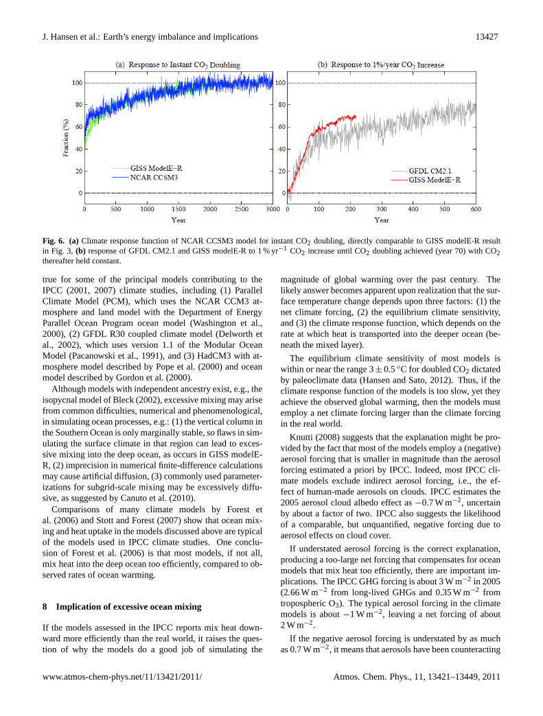
The response function of the NCAR CCSM3 model (Kiehlet al., 2006) can be compared directly with the response func-tion of the GISS model (Fig. 3) and GFDL and GISS modelresponses to a 1 % yr−1 CO2 forcing are available (Fig. 6b).Equilibrium sensitivities of these specific NCAR and GFDLmodels are 2.5◦C and 3.4◦C, respectively, which comparesto 3.0◦C for the GISS model. It is clear from Fig. 6 thatocean mixing slows the surface temperature response aboutas much in the other two models as in the GISS model, withthe differences being consistent with their moderate differ-ences in equilibrium sensitivity. Data provided by J. Gre-gory (personal communication, 2008) for a 1200-yr run ofthe UK Hadley Centre model (Gordon et al., 2000) imply astill longer response time for that model, which is consistentwith comparably efficient mixing of heat into the deep ocean,given the greater climate sensitivity of that model (about10◦C for quadrupled CO2, which is a forcing∼8 W m−2).
One plausible explanation for why many models have sim-ilarly slow response functions is common ancestry. Theocean component of many atmosphere-ocean climate mod-els is the GFDL Bryan-Cox ocean model (Bryan, 1969;Cox, 1984). Common ancestry of the ocean sub-model is
Atmos. Chem. Phys., 11, 13421–13449, 2011 www.atmos-chem-phys.net/11/13421/2011/
J. Hansen et al.: Earth’s energy imbalance and implications 13427
Fig. 6. (a) Climate response function of NCAR CCSM3 model for instant CO2 doubling, directly comparable to GISS modelE-R result in Fig. 3, (b) response of GFDL CM2.1 and GISS modelE-R to 1%/year CO2 increase until CO2 doubling achieved (year 70) with CO2 thereafter held constant.
3
Fig. 6. (a) Climate response function of NCAR CCSM3 model for instant CO2 doubling, directly comparable to GISS modelE-R resultin Fig. 3, (b) response of GFDL CM2.1 and GISS modelE-R to 1 % yr−1 CO2 increase until CO2 doubling achieved (year 70) with CO2thereafter held constant.
true for some of the principal models contributing to theIPCC (2001, 2007) climate studies, including (1) ParallelClimate Model (PCM), which uses the NCAR CCM3 at-mosphere and land model with the Department of EnergyParallel Ocean Program ocean model (Washington et al.,2000), (2) GFDL R30 coupled climate model (Delworth etal., 2002), which uses version 1.1 of the Modular OceanModel (Pacanowski et al., 1991), and (3) HadCM3 with at-mosphere model described by Pope et al. (2000) and oceanmodel described by Gordon et al. (2000).
Although models with independent ancestry exist, e.g., theisopycnal model of Bleck (2002), excessive mixing may arisefrom common difficulties, numerical and phenomenological,in simulating ocean processes, e.g.: (1) the vertical column inthe Southern Ocean is only marginally stable, so flaws in sim-ulating the surface climate in that region can lead to exces-sive mixing into the deep ocean, as occurs in GISS modelE-R, (2) imprecision in numerical finite-difference calculationsmay cause artificial diffusion, (3) commonly used parameter-izations for subgrid-scale mixing may be excessively diffu-sive, as suggested by Canuto et al. (2010).
Comparisons of many climate models by Forest etal. (2006) and Stott and Forest (2007) show that ocean mix-ing and heat uptake in the models discussed above are typicalof the models used in IPCC climate studies. One conclu-sion of Forest et al. (2006) is that most models, if not all,mix heat into the deep ocean too efficiently, compared to ob-served rates of ocean warming.
8 Implication of excessive ocean mixing
If the models assessed in the IPCC reports mix heat down-ward more efficiently than the real world, it raises the ques-tion of why the models do a good job of simulating the
magnitude of global warming over the past century. Thelikely answer becomes apparent upon realization that the sur-face temperature change depends upon three factors: (1) thenet climate forcing, (2) the equilibrium climate sensitivity,and (3) the climate response function, which depends on therate at which heat is transported into the deeper ocean (be-neath the mixed layer).
The equilibrium climate sensitivity of most models iswithin or near the range 3± 0.5◦C for doubled CO2 dictatedby paleoclimate data (Hansen and Sato, 2012). Thus, if theclimate response function of the models is too slow, yet theyachieve the observed global warming, then the models mustemploy a net climate forcing larger than the climate forcingin the real world.
Knutti (2008) suggests that the explanation might be pro-vided by the fact that most of the models employ a (negative)aerosol forcing that is smaller in magnitude than the aerosolforcing estimated a priori by IPCC. Indeed, most IPCC cli-mate models exclude indirect aerosol forcing, i.e., the ef-fect of human-made aerosols on clouds. IPCC estimates the2005 aerosol cloud albedo effect as−0.7 W m−2, uncertainby about a factor of two. IPCC also suggests the likelihoodof a comparable, but unquantified, negative forcing due toaerosol effects on cloud cover.
If understated aerosol forcing is the correct explanation,producing a too-large net forcing that compensates for oceanmodels that mix heat too efficiently, there are important im-plications. The IPCC GHG forcing is about 3 W m−2 in 2005(2.66 W m−2 from long-lived GHGs and 0.35 W m−2 fromtropospheric O3). The typical aerosol forcing in the climatemodels is about−1 W m−2, leaving a net forcing of about2 W m−2.
If the negative aerosol forcing is understated by as muchas 0.7 W m−2, it means that aerosols have been counteracting
www.atmos-chem-phys.net/11/13421/2011/ Atmos. Chem. Phys., 11, 13421–13449, 2011

13428 J. Hansen et al.: Earth’s energy imbalance and implications
half or more of the GHG forcing. In that event, humanityhas made itself a Faustian bargain more dangerous than com-monly supposed.
9 Ambiguity between aerosols and ocean mixing
Uncertainties in aerosol forcing and ocean mixing (climateresponse function) imply that there is a family of solutionsconsistent with observed global warming. The range of ac-ceptable solutions is explored in Fig. 7 via Green’s func-tion calculations that employ the three response functions ofFig. 5. The slow response, based on GISS modelE-R, is typi-cal of most IPCC models. The fast response is a lower boundon mixing into the deep ocean. The intermediate responseis a conjecture influenced by knowledge of excessive oceanmixing in GISS modelE-R. Temporal variation of aerosolforcing is assumed to be proportional to the aerosol forcing inFig. 1a. We seek the value of a factor (“constant”) multiply-ing this aerosol forcing history that yields closest agreementwith the observed temperature record. In a later section wewill discuss uncertainties in the shape of the aerosol forcinghistory in Fig. 1a.
Values of constant providing best least-squares fit for1880–2010 are 0.84, 1.05 and 1.20 for the slow, intermedi-ate and fast response functions. This entire record may givetoo much weight to the late 1800s, when the volcanic aerosoloptical depth from Krakatau and other volcanoes is very un-certain and the global temperature record is also least certain.Thus we also found the values of constant providing best fitfor the period 1950–2010: 0.68, 0.97 and 1.16 for the slow,intermediate and fast response functions. The least-squareserror curves are quite flat-bottomed, so intermediate valuesfor constant: 0.75, 1 and 1.2 fit the observed temperaturecurve nearly as well for both periods as the values optimizedfor a single period.
Thus the aerosol forcing that provides best agreement withobserved global temperature for the slow response function(deep ocean mixing) is−1.2 W m−2. The best fit aerosolforcings are−1.6 and−2.0 W m−2 for the intermediate andfast response functions.
Given that two major uncertainties (aerosol forcing andocean mixing) affect expected global warming, solution ofthe problem requires a second criterion, in addition to globaltemperature. The planetary energy imbalance (Hansen et al.,1997, 2005) is the fundamental relevant quantity, because itis a direct consequence of the net climate forcing.
Expected planetary energy imbalance for any given cli-mate forcing scenario and ocean mixing (climate responsefunction) follows from the above Green’s function calcula-tion:
Planetary Energy Imbalance(t) =
F ×(1Teq−1T )/1Teq= F −1T/S. (3)
This equation is simply a statement of the fact that the en-ergy imbalance is the portion of the climate forcing that the
planet’s surface temperature has not yet responded to.1Teq,1T andF in this equation are all functions of time.1Teq,the equilibrium temperature change for the climate forcingthat existed at timet , is the product of the climate forcing attime t and the fast-feedback climate sensitivity,S ×F , withS ∼ 3/4
◦C per W m−2. 1T is the global surface temperatureat time t calculated with the Green’s function (2). Planetaryenergy imbalance calculated from Eq. (3) agrees closely withglobal climate model simulations (Hansen et al., 2007).
Equation (3) with1Teq andS defined to include only fastfeedbacks is valid for time scales from decades to a cen-tury, a period short enough that the size of the ice sheets willnot change significantly. The climate forcing,F , is definedto include all changes of long-lived gases including thosethat arise from slow carbon cycle feedbacks that affect at-mospheric composition, such as those due to changing oceantemperature or melting permafrost.
Calculated planetary energy imbalance for the three oceanmixing rates, based on Eq. (3), are shown in the right halfof Fig. 7. The slow response function, relevant to most cli-mate models, has a planetary energy imbalance∼ 1 W m−2
in the first decade of the 21st century. The fast responsefunction has an average energy imbalance∼0.35 W m−2 inthat decade. The intermediate climate response function fallsabout half way between these extremes.
Discrimination among these alternatives requires observa-tions of changing ocean heat content. Ocean heat data priorto 1970 are not sufficient to produce a useful global aver-age, and data for most of the subsequent period are stillplagued with instrumental error and poor spatial coverage,especially of the deep ocean and the Southern Hemisphere,as quantified in analyses and error estimates by Domingueset al. (2008) and Lyman and Johnson (2008).
Dramatic improvement in knowledge of Earth’s energyimbalance is possible this decade as Argo float observations(Roemmich and Gilson, 2009) are improved and extended.If Argo data are complemented with adequate measurementsof climate forcings, we will argue, it will be possible to as-sess the status of the global climate system, the magnitudeof global warming in the pipeline, and the change of climateforcing that is required to stabilize climate.
10 Observed planetary energy imbalance
As ocean heat data improve, it is relevant to quantify smallerterms in the planet’s energy budget. Levitus et al. (2005),Hansen et al. (2005a) and IPCC (2007) estimated past multi-decadal changes of small terms in Earth’s energy imbalance.Recently improved data, including satellite measurements ofice, make it possible to tabulate many of these terms on anannual basis. These smaller terms may become increasinglyimportant, especially if ice melting continues to increase, socontinued satellite measurements are important.
Atmos. Chem. Phys., 11, 13421–13449, 2011 www.atmos-chem-phys.net/11/13421/2011/

J. Hansen et al.: Earth’s energy imbalance and implications 13429
Fig. 7. Green's function calculation of surface temperature change and planetary energy imbalance. Three choices for climate response function are slow (top row, same as GISS modelE-R), intermediate (middle) and fast response (bottom). Factor "constant" multiplies aerosol forcing of Fig. 1.
4
Fig. 7. Green’s function calculation of surface temperature change and planetary energy imbalance. Three choices for climate responsefunction are slow (top row, same as GISS modelE-R), intermediate (middle) and fast response (bottom). Factor “constant” multiplies aerosolforcing of Fig. 1.
Our units for Earth’s energy imbalance are W m−2 aver-aged over Earth’s entire surface (∼5.1× 10¹⁴ m2). Notethat 1 watt-yr for the full surface of Earth is∼1.61× 10²² J(joules).
10.1 Non-ocean terms in planetary energy imbalance
The variability of annual changes of heat content is large, butsmoothing over several years allows trends to be seen. For
consistency with the analysis of Argo data, we calculate 6-yr moving trends of heat uptake for all of the terms in theplanetary energy imbalance.
Atmosphere. The small atmospheric heat capacity con-tributes a small variable term to Earth’s energy imbalance(Fig. 8a). Because the term is small, we obtain it simply asthe product of the surface air temperature change (Hansenet al., 2010), the mass of the atmosphere (∼5.13× 10¹⁸ kg),and its heat capacitycp ∼ 1000 J (kg K)−1. The fact that
www.atmos-chem-phys.net/11/13421/2011/ Atmos. Chem. Phys., 11, 13421–13449, 2011

13430 J. Hansen et al.: Earth’s energy imbalance and implications
Fig. 8. Contributions to planetary energy imbalance by processes other than ocean heat uptake. Annual data are smoothed with moving 6-year linear trends.
Fig. 9. (a) Sum of non-ocean contributions to planetary energy imbalance from Fig. 8, (b) Six-year trends of ocean heat uptake estimated by Levitus et al. (2009) and Lyman et al. (2010) for upper 700 m of the ocean, and estimates based on Argo float data for the upper 2000 m for 2003-2008 and 2005-2010.
5
Fig. 8. Contributions to planetary energy imbalance by processes other than ocean heat uptake. Annual data are smoothed with moving 6-yrlinear trends.
upper tropospheric temperature change tends to exceed sur-face temperature change is offset by stratospheric coolingthat accompanies tropospheric warming. Based on simulatedchanges of atmospheric temperature profile (IPCC, 2007;Hansen et al., 2005b), our use of surface temperature changeto approximate mean atmospheric change modestly over-states heat content change.
IPCC (2007) in their Fig. 5.4 has atmospheric heat gainas the second largest non-ocean term in the planetary en-ergy imbalance at 5× 10²¹ J for the period 1961–2003. Lev-itus et al. (2001) has it even larger at 6.6× 10²¹ J for theperiod 1955–1996. Our calculation yields 2.5× 10²¹ J for1961–2003 and 2× 10²¹ J for 1955–1996. We could not findsupport for the larger values of IPCC (2007) and Levitus etal. (2001) in the references that they provided. The latentenergy associated with increasing atmospheric water vaporin a warmer atmosphere is an order of magnitude too smallto provide an explanation for their high estimates of atmo-spheric heat gain.
Land. We calculate transient ground heat uptake for theperiod 1880–2009 employing the standard one-dimensionalheat conduction equation. Calculations went to a depth of200 m, which is sufficient to capture heat content changeon the century time scale. We used global average valuesof thermal diffusivity, mass density, and specific heat from
Whittington et al. (2009). Temperature changes of the sur-face layer were driven by the global-land mean temperaturechange in the GISS data set (Hansen et al., 2010); a graph ofglobal-land temperature is available athttp://www.columbia.edu/∼mhs119/Temperature/TmoreFigs/.
Our calculated ground heat uptake (Fig. 8b) is in the rangeof other estimates. For the period 1901–2000 we obtain∼12.6× 10²¹ J; Beltrami et al. (2002) give∼15.9× 10²¹ J;Beltrami (2002) gives∼13× 1021 J; Huang (2006) gives10.3× 1021 J. Differences among these analyses are largelydue to alternative approaches for deriving surface heat fluxesas well as alternative choices for the thermal parameters men-tioned above (ours being based on Whittington et al., 2009).Our result is closest to that of Beltrami (2002), who derivedland surface flux histories and heat gain directly from bore-hole temperature profiles (using a greater number of profilesthan Beltrami et al., 2002).
Ice on land. We use gravity satellite measurements ofmass changes of the Greenland and Antarctic ice sheets(Velicogna, 2009). For the period prior to gravity satel-lite data we extrapolate backward to smaller Greenland andAntarctic mass loss using a 10-yr doubling time. AlthoughHansen and Sato (2012) showed that the satellite record istoo short to well-define a curve for mass loss versus time,the choice to have mass loss decrease rapidly toward earlier
Atmos. Chem. Phys., 11, 13421–13449, 2011 www.atmos-chem-phys.net/11/13421/2011/

J. Hansen et al.: Earth’s energy imbalance and implications 13431
times is consistent with a common glaciological assumptionthat the ice sheets were close to mass balance in the 1990s(Zwally et al., 2011). Our calculations for the energy associ-ated with decreased ice mass assumes that the ice begins at−10◦C and eventually reaches a mean temperature +15◦C,but most of the energy is used in the phase change from iceto water.
Mass loss by small glaciers and ice caps is taken as theexponential fit to data in Fig. 1 of Meier et al. (2007) up to2005 and as constant thereafter.
Floating ice. Change of Arctic sea ice volume (Rothrocket al., 2008) is taken from (http://psc.apl.washington.edu/ArcticSeaiceVolume/IceVolume.php), data on the Univer-sity of Washington Polar Science Center web site. Changeof Antarctic sea ice area is from the National Snow andIce Data Center (http://nsidc.org/data/seaiceindex/archives/index.html), with thickness of Antarctic ice assumed to beone meter. Antarctic sea ice volume changes, and heat con-tent changes, are small compared to the Arctic change.
We use the Shepherd et al. (2010) estimate for change ofice shelf volume, which yields a very small ice shelf contri-bution to planetary energy imbalance (Fig. 8d). AlthoughShepherd et al. (2010) have numerous ice shelves losingmass, with Larsen B losing an average of 100 cubic kilo-meters per year from 1998 to 2008, they estimate that theFilchner-Ronne, Ross, and Amery ice shelves are gainingmass at a combined rate of more than 350 cubic kilome-ters per year due to a small thickening of these large-areaice shelves.
Summary.Land warming (Fig. 8b) has been the largest ofthe non-ocean terms in the planetary energy imbalance overthe past few decades. However, contributions from meltingpolar ice are growing rapidly. The very small value for iceshelves, based on Shepherd et al. (2010), seems question-able, depending very sensitively on estimated changes of thethickness of the large ice shelves. The largest ice shelves andthe ice sheets could become major contributors to energy im-balance, if they begin to shed mass more rapidly. Because ofthe small value of the ice shelf term, we have neglected thelag between the time of ice shelf break-up and the time ofmelting, but this lag may become significant with major iceshelf breakup.
The sum of non-ocean contributions to the planetary en-ergy imbalance is shown in Fig. 9a. This sum is still small,less than 0.1 W m−2, but growing.
10.2 Ocean term in planetary energy imbalance
Because of the ocean’s huge heat capacity, temperaturechange must be measured very precisely to determine theocean’s contribution to planetary energy imbalance. Ade-quate precision is difficult to attain because of spatial andtemporal sparseness of data, regional and seasonal biases inobservations, and changing proportions of data from vari-ous instrument types with different biases and inaccuracies
(Harrison and Carson, 2007; Domingues et al., 2008; Lymanand Johnson, 2008; Roemmich and Gilson 2009; Purkey andJohnson, 2010).
It has been possible to identify and adjust for some instru-mental biases (Gouretski and Koltermann, 2007; Wijffels etal., 2008; Levitus et al., 2009). These ameliorations havebeen shown to reduce what otherwise seemed to be unreal-istically large decadal variations of ocean heat content (Do-minigues et al., 2008). However, analyses of ocean heat up-take by different investigators (Levitus et al., 2009; Lyman etal., 2010; Church et al., 2011) differ by as much as a factor oftwo even in the relatively well-sampled period 1993–2008.
Limitations in the spatial sampling and quality of histor-ical ocean data led to deployment in the past decade of theinternational array of Argo floats capable of measurementsto 2000 m (Roemmich and Gilson, 2009). Even this well-planned program had early instrumental problems causingdata biases (Willis et al., 2007), but it was possible to identifyand eliminate problematic data. Lyman and Johnson (2008)show that by about 2004 the Argo floats had sufficient space-time sampling to yield an accurate measure of heat contentchange in the upper ocean.
Graphs of ocean heat content usually show cumulativechange. The derivative of this curve, the annual change ofheat content, is more useful for our purposes, even thoughit is inherently “noisy”. The rate of ocean heat uptake de-termines the planetary energy imbalance, which is the mostfundamental single measure of the state of Earth’s climate.The planetary energy imbalance is the drive for future cli-mate change and it is simply related to climate forcings, be-ing the portion of the net climate forcing that the planet hasnot yet responded to.
The noisiness of the annual energy imbalance is reducedby appropriate smoothing over several years. Von Schuck-mann and Le Traon (2011) calculate a weighted linear trendfor the 6-yr period of most complete data, 2005–2010, theweight accounting for modest improvement in spatial cov-erage of observations during the 6-yr period. They ob-tain a heat content trend of 0.54± 0.1 W m−2 with analy-sis restricted to depths 10–1500 m and latitudes 60◦ N–60◦ S,equivalent to 0.38± 0.07 W m−2 globally, assuming simi-lar heat uptake at higher latitude ocean area2. Repeatingtheir analysis for 0–2000 m yields 0.59 W m−2, equivalent to0.41 W m−2 globally.
The uncertainty (standard error) for the von Schuckmannand Le Traon (2011) analyses does not include possible re-maining systematic biases in the Argo observing system suchas uncorrected drift of sensor calibration or pressure errors.A recent study of Barker et al. (2011) underscores the needfor careful analyses to detect and to remove systematic errors
2 Ocean surface south of 60◦ S and north of 60◦ N cover 4 per-cent and 3 percent of Earth’s surface, respectively. These latituderegions contain 5.4 percent and 1.6 percent of the ocean’s volume,respectively.
www.atmos-chem-phys.net/11/13421/2011/ Atmos. Chem. Phys., 11, 13421–13449, 2011

13432 J. Hansen et al.: Earth’s energy imbalance and implications
Fig. 8. Contributions to planetary energy imbalance by processes other than ocean heat uptake. Annual data are smoothed with moving 6-year linear trends.
Fig. 9. (a) Sum of non-ocean contributions to planetary energy imbalance from Fig. 8, (b) Six-year trends of ocean heat uptake estimated by Levitus et al. (2009) and Lyman et al. (2010) for upper 700 m of the ocean, and estimates based on Argo float data for the upper 2000 m for 2003-2008 and 2005-2010.
5
Fig. 9. (a)Sum of non-ocean contributions to planetary energy imbalance from Fig. 8,(b) six-yr trends of ocean heat uptake estimated byLevitus et al. (2009) and Lyman et al. (2010) for upper 700 m of the ocean, and estimates based on Argo float data for the upper 2000 m for2003–2008 and 2005–2010.
in ocean observations. Such biases caused significant errorsin prior analyses. Estimated total uncertainty including un-known biases is necessarily subjective, but it is included inour summary below of all contributions to the planetary en-ergy imbalance.
We emphasize the era of Argo data because of its po-tential for accurate analysis. For consistency with the vonSchuckmann and Le Traon (2011) analysis we smooth otherannual data with a 6-yr moving linear trend. The 6-yrsmoothing is a compromise between minimizing the errorand allowing temporal change due to events such as thePinatubo volcano and the solar cycle to remain apparent inthe record.
Heat uptake in the upper 700 m of the ocean (Fig. 9b)has been estimated by Lyman et al. (2010) and Levitus etal. (2009). The 1993–2008 period is of special interest, be-cause satellite altimetry for that period allows accurate mea-surement of sea level change.
Lyman et al. (2010) estimate average 1993–2008 heat gainin the upper 700 m of the ocean as 0.64± 0.11 W m−2, wherethe uncertainty range is the 90 percent confidence interval.The error analysis of Lyman et al. (2010) includes uncer-tainty due to mapping choice, instrument (XBT) bias correc-tion, quality control choice, sampling error, and climatologychoice. Lyman and Johnson (2008) and Lyman et al. (2010)describe reasons for their analysis choices, most significantlythe weighted averaging method for data sparse regions.
Levitus and colleagues (Levitus et al., 2000, 2005, 2009)maintain a widely used ocean data set. Lyman andJohnson (2008) suggest that the Levitus et al. objective anal-ysis combined with simple volumetric integration in analyz-ing ocean heat uptake allows temperature anomalies to relaxtoward zero in data sparse regions and thus tends to underes-timate ocean heat uptake. However, the oceanographic com-munity has not reached consensus on a best analysis of exist-ing data, so we compare our calculations with both Levituset al. (2009) and Lyman et al. (2010).
Lyman et al. (2010) and Levitus et al. (2009) find smallerheat gain in the upper 700 m in the Argo era than that found inthe upper 2000 m by von Schuckmann and Le Traon (2011),as expected3. Although the accuracy of ocean heat uptakein the pre-Argo era is inherently limited, it is likely that heatuptake in the Argo era is smaller than it was during the 5–10 yr preceding full Argo deployment, as discussed by Tren-berth (2009, 2010) and Trenberth and Fasullo (2010).
Heat uptake at ocean depths below those sampled by Argois small, but not negligible. Purkey and Johnson (2010)find the abyssal ocean (below 4000 m) gaining heat at rate0.027± 0.009 W m−2 (average for entire globe) in the pastthree decades. Purkey and Johnson (2010) show that mostof the global ocean heat gain between 2000 m and 4000 moccurs in the Southern Ocean south of the Sub-AntarcticFront. They estimate the rate of heat gain in the deepSouthern Ocean (depths 1000–4000 m) during the past threedecades4 to be 0.068± 0.062 W m−2. The uncertaintiesgiven by Purkey and Johnson (2010) for the abyssal oceanand Southern Ocean heat uptake are the uncertainties for95 percent confidence. Additional observations available forthe deep North Atlantic, not employed in the Purkey andJohnson (2010) method of repeat sections, could be broughtto bear for more detailed analysis of that ocean basin, but be-cause of its moderate size the global energy balance is notlikely to be substantially altered.
3 von Schuckmann and Le Traon (2011) find heat gain0.44± 0.1, 0.54± 0.1 and 0.59± 0.1 W m−2 for ocean depths 0–700 m, 10–1500 m, and 0–2000 m, respectively, based on 2005–2010 trends. Multiply by 0.7 for global imbalance.
4 The data span 1981–2010, but the mean time was 1992 for thefirst sections and 2005 for the latter sections, so the indicated fluxmay best be thought of as the mean for the interval 1992–2005.
Atmos. Chem. Phys., 11, 13421–13449, 2011 www.atmos-chem-phys.net/11/13421/2011/

J. Hansen et al.: Earth’s energy imbalance and implications 13433
Fig.10. (a) Estimated contributions to planetary energy imbalance in 1993-2008, and (b) in 2005-2010. Except for heat gain in the abyssal ocean and Southern Ocean, ocean heat change beneath the upper ocean (top 700 m for period 1993-2008, top 2000 m in period 2005-2010) is assumed to be small and is not included. Data sources are the same as for Figs. 8 and 9. Vertical whisker in (a) is not an error bar, but rather shows the range between the Lyman et al. (2010) and Levitus et al. (2009) estimates. Error bar in (b) combines estimated errors of von Schuckmann and Le Traon (2011) and Purkey and Johnson (2010).
6
Fig. 10. (a)Estimated contributions to planetary energy imbalance in 1993–2008, and(b) in 2005–2010. Except for heat gain in the abyssalocean and Southern Ocean, ocean heat change beneath the upper ocean (top 700 m for period 1993–2008, top 2000 m in period 2005–2010)is assumed to be small and is not included. Data sources are the same as for Figs. 8 and 9. Vertical whisker in(a) is not an error bar, butrather shows the range between the Lyman et al. (2010) and Levitus et al. (2009) estimates. Error bar in(b) combines estimated errors ofvon Schuckmann and Le Traon (2011) and Purkey and Johnson (2010).
10.3 Summary of contributions to planetary energyimbalance
Knowledge of Earth’s energy imbalance becomes increas-ingly murky as the period extends further into the past. Ourchoice for starting dates for summary comparisons (Fig. 10)is (a) 1993 for the longer period, because sea level began tobe measured from satellites then, and (b) 2005 for the shorterperiod, because Argo floats had achieved nearly full spatialcoverage.
Observed planetary energy imbalance includes upperocean heat uptake plus three small terms. The first term isthe sum of non-ocean terms (Fig. 9a). The second term, heatgain in the abyssal ocean (below 4000 m), is estimated to be0.027± 0.009 W m−2 by Purkey and Johnson (2010), basedon observations in the past three decades. Deep ocean heatchange occurs on long time scales and is expected to increase(Wunsch et al., 2007). Because global surface temperatureincreased almost linearly over the past three decades (Hansenet al., 2010) and deep ocean warming is driven by surfacewarming, we take this rate of abyssal ocean heat uptake asconstant during 1980–present. The third term is heat gainin the ocean layer between 2000 and 4000 m for which weuse the estimate 0.068± 0.061 W m−2 of Purkey and John-son (2010).
Upper ocean heat storage dominates the planetary energyimbalance during 1993–2008. Ocean heat change below700 m depth in Fig. 10 is only for the Southern and abyssaloceans, but those should be the largest supplements to up-per ocean heat storage (Leuliette and Miller, 2009). Levi-tus et al. (2009) depth profiles of ocean heat gain suggestthat 15–20 percent of ocean heat uptake occurs below 700 m,which would be mostly accounted for by the estimates for
the Southern and abyssal oceans. Uncertainty in total oceanheat storage during 1993–2008 is dominated by the discrep-ancy at 0–700 m between Levitus et al. (2009) and Lyman etal. (2010).
The Lyman et al. (2010) upper ocean heat storage of0.64± 0.11 W m−2 for 1993–2008 yields planetary energyimbalance 0.80 W m−2. The smaller upper ocean heat gainof Levitus et al. (2009), 0.41 W m−2, yields planetary energyimbalance 0.57 W m−2.
The more recent period, 2005–2010, has smaller upperocean heat gain, 0.38 W m−2 for depths 10–1500 m (vonSchuckmann and Le Traon, 2011) averaged over the entireplanetary surface and 0.41 W m−2 for depths 0–2000 m. Thetotal planetary imbalance in 2005–2010 is 0.58 W m−2. Non-ocean terms contribute 13 percent of the total heat gain in thisperiod, exceeding the contribution in the longer period in partbecause of the increasing rate of ice melt.
Estimates of standard error of the observed planetary en-ergy imbalance are necessarily partly subjective because theerror is dominated by uncertainty in ocean heat gain, in-cluding imperfect instrument calibrations and the possibil-ity of unrecognized biases. The von Schuckmann and LeTraon (2011) error estimate for the upper ocean (0.1 W m−2)
is 0.07 W m−2 for the globe, excluding possible remainingsystematic biases in the Argo observing system (see alsoBarker et al., 2011). Non-ocean terms (Fig. 8) contributelittle to the total error because the terms are small and welldefined. The error contribution from estimated heat gainin the deep Southern and abyssal oceans is also small, be-cause the values estimated by Purkey and Johnson (2010) forthese terms, 0.062 and 0.009 W m−2, respectively, are their95 percent (2-σ) confidence limits.
www.atmos-chem-phys.net/11/13421/2011/ Atmos. Chem. Phys., 11, 13421–13449, 2011

13434 J. Hansen et al.: Earth’s energy imbalance and implications
Our estimated planetary energy imbalance is0.80± 0.20 W m−2 for 1993–2008 and 0.58± 0.15 W m−2
for 2005–2010, with estimated 1-σ standard error. Our esti-mate for 1993–2008 uses the Lyman et al. (2010) ocean heatgain rather than Levitus et al. (2009) for the reason discussedin Sect. 11. These error estimates may be optimistic becauseof the potential for unrecognized systematic errors, indeedChurch et al. (2011) estimate an ocean heat uptake of only0.33 W m−2 for 1993–2008. For this reason, our conclusionsin this paper are based almost entirely on analyses of theperiod with the most complete data, 2005–2010. Samplingerror in the Argo era will decline as the Argo record length-ens (von Schuckmann and Le Traon, 2011), but systematicbiases may remain and require continued attention.
11 Modeled versus observed planetary energyimbalance
Observed and simulated planetary energy imbalances(Fig. 11) are both smoothed via moving 6-yr trends for com-parison with the Argo analysis. The three small energy bal-ance terms described above are added to the observed upperocean heat uptake.
Argo era observed planetary energy imbalances are0.70 W m−2 in 2003–2008 and 0.58 W m−2 in 2005–2010.Slow, intermediate, and fast response functions yield plane-tary energy imbalances 0.95, 0.59 and 0.34 W m−2 in 2003–2008 and 0.98, 0.61 and 0.35 W m−2 in 2005–2010.
Observed planetary energy imbalance in 1993–2008 is0.80 W m−2, assuming the Lyman et al. (2010) upper oceanheat storage, but only 0.59 W m−2 with the Levitus etal. (2009) analysis. The calculated planetary energy imbal-ance for 1993–2008 is 1.06, 0.74 and 0.53 W m−2 for theslow, intermediate and fast climate response functions, re-spectively.
We conclude that the slow climate response function isinconsistent with the observed planetary energy imbalance.This is an important conclusion because it implies that manyclimate models have been using an unrealistically large netclimate forcing and human-made atmospheric aerosols prob-ably cause a greater negative forcing than commonly as-sumed.
The intermediate response function yields planetary en-ergy imbalance in close agreement with Argo-era observa-tions. The intermediate response function also agrees withthe planetary energy imbalance for 1993–2008, if we acceptthe Lyman et al. (2010) estimate for upper ocean heat up-take. Given that (1) Lyman et al. (2010) data is in muchbetter agreement with the Argo-era analyses of von Schuck-mann et al., and (2) a single response function must fit boththe Argo-era and pre-Argo-era data, these results support thecontention that the Levitus et al. analysis understates oceanheat uptake in data sparse regions. However, note that theconclusion that the slow response function is incompatible
Fig.10. (a) Estimated contributions to planetary energy imbalance in 1993-2008, and (b) in 2005-2010. Except for heat gain in the abyssal ocean and Southern Ocean, ocean heat change beneath the upper ocean (top 700 m for period 1993-2008, top 2000 m in period 2005-2010) is assumed to be small and is not included. Data sources are the same as for Figs. 8 and 9. Vertical whisker in (a) is not an error bar, but rather shows the range between the Lyman et al. (2010) and Levitus et al. (2009) estimates. Error bar in (b) combines estimated errors of von Schuckmann and Le Traon (2011) and Purkey and Johnson (2010).
6
Fig. 11. Observed and calculated planetary energy imbalance,smoothed with moving 6-yr trend. Non-ocean terms of Fig. 9a andsmall contributions of the abyssal ocean and deep Southern Ocean,as discussed in the text, are added to the upper ocean heat contentanalyses of Levitus et al. (2009), Lyman et al. (2010), von Schuck-mann et al. (2009), and von Schuckmann and Le Traon (2011).Results for slow, intermediate, and fast climate response functionseach fit the observed temperature record (Fig. 7).
with observed planetary energy imbalance does not requireresolving the difference between the Lyman et al. and Levi-tus et al. analyses.
Our principal conclusions, that the slow response func-tion is unrealistically slow, and thus the corresponding nethuman-made climate forcing is unrealistically large, are sup-ported by implications of the slow response function forocean mixing. The slow response model requires a largenet climate forcing (∼2.1 W m−2 in 2010) to achieve globalsurface warming consistent with observations, but that largeforcing necessarily results in a large amount of heat beingmixed into the deep ocean. Indeed, GISS modelE-R achievesrealistic surface warming (Hansen et al., 2007b), but heat up-take by the deep ocean exceeds observations. Quantitativestudies will be reported by others (A. Romanou and J. Mar-shall, personal communication, 2011) confirming that GISSmodelE-R has excessive deep ocean uptake of heat and pas-sive tracers such as CFCs. Excessive deep mixing, especiallyin the Southern Ocean, seems to occur in many ocean models(Dutay et al., 2002; Gent et al., 2006; Griffies et al., 2009).
12 Is there closure with observed sea level change?
Munk (2002, 2003) drew attention to the fact that melting iceand thermal expansion of the ocean did not seem to be suffi-cient to account for observed sea level rise. This issue nowcan be reexamined with the help of Argo data and improvingdata on the rate of ice melt.
Sea level in the period of satellite observations increasedat an average rate 3.2± 0.4 mm yr−1 (Fig. 12). In the sixyear period of the most accurate Argo data, 2005–2010, sealevel increased 2.0± 0.5 mm yr−1. The slower recent rate of
Atmos. Chem. Phys., 11, 13421–13449, 2011 www.atmos-chem-phys.net/11/13421/2011/

J. Hansen et al.: Earth’s energy imbalance and implications 13435
. Fig. 12. Sea level change based on satellite altimeter measurements calibrated with tide-gauge measurements (Nerem et al., 2006; data updates at http://sealevel.colorado.edu/).
Fig. 13. (a) Percent of latitude-depth space occupied by water, (b) thermal expansion coefficient of water in today's ocean, (c) product of the quantities in (a) and (b). Equal intervals of the latitude scale have equal surface area. Calculations are area-weighted. Latitude ranges 90-60S, 60-30S, 30S-0, 0-30N, 30-60N, 60-90N contain 5, 26, 28, 27, 12, 2 percent of the ocean mass, and ocean surface in these latitude belts cover 4, 17, 19, 18, 9, 3 percent of the global surface area, respectively.
7
Fig. 12.Sea level change based on satellite altimeter measurementscalibrated with tide-gauge measurements (Nerem et al., 2006; dataupdates athttp://sealevel.colorado.edu/).
sea level rise may be due in part to the strong La Nina in2010, as there is a strong correlation of global sea level andENSO (Nerem et al., 2010). One facet of ENSO variability isvertical redistribution of heat, with the warmer surface layersof the El Nino phase causing a loss of ocean heat content andthe opposite effect during La Ninas (Roemmich and Gilson,2011). Another facet is storage of water on continents duringLa Nina as a consequence of heavy rainfall and floods (Llovelet al., 2011).
The potential of different volumes of the ocean to con-tribute to sea level rise via thermal expansion is examined inFig. 13, which has horizontal axis proportional to cosine oflatitude, so that equal increments have equal surface area onthe planet. Movement of heat from the tropical-subtropicalupper ocean to greater depths, or especially to higher lati-tudes, by itself causes global sea level fall (Fig. 13b). Thequantity in Fig. 13c must be multiplied by temperaturechange to find the contribution to ocean thermal expansion.Observed temperature change is largest in the upper few hun-dred meters of the ocean, which thus causes most of the sealevel rise due to thermal expansion. Observed warming ofthe deep Southern Ocean and the abyssal ocean contributes asmall amount to sea level rise (Purkey and Johnson, 2010).
Ocean temperature change in the upper 1500 mduring 2005–2010 caused thermal expansion of0.75± 0.15 mm yr−1 (von Schuckmann and Le Traon,2011). Warming of the deep (1500–4000 m) SouthernOcean and the abyssal ocean during the past three decadescontributed at rates, respectively, 0.073± 0.067 and0.053± 0.017 mm yr−1 (Purkey and Johnson, 2010)5. Be-cause global surface temperature increased almost linearly in
5 This sea level rise due to Southern Ocean thermal expansiondiffers slightly from the published value as S. Purkey kindly re-computed this term (personal communication, 2011) to eliminateoverlap with Argo data.
recent decades (Hansen et al., 2010) and deep ocean warm-ing is driven by surface warming, we take this mean rate ofdeep ocean warming as our estimate for these small terms.Thus thermal expansion in the Argo period contributes about0.88 mm yr−1 to sea level rise. Thus our estimate of thermalexpansion in the Argo era is 0.88 mm yr−1, the same as theChurch et al. (2011) estimate (0.88± 0.33 mm yr−1) for theperiod 1993–2008.
Satellite measurement of Earth’s changing gravity fieldshould eventually allow accurate quantification of the princi-pal contributions of ice melt to sea level rise. But at presentthere is a range of estimates due in part to the difficultyof disentangling ice mass loss from crustal isostatic adjust-ment (Bromwich and Nicolas, 2010; Sorensen and Forsberg,2010; Wu et al., 2010). The “high” estimates in Fig. 14 forGreenland and Antarctica, respectively, 281 and 176 Gt yr−1
(360 Gt= 1 mm sea level), are from Velicogna (2009). A re-cent analysis (Rignot et al., 2011), comparing surface massbudget studies and the gravity method, supports the high es-timates of Velicogna (2009). The low estimate for Green-land, 104 Gt yr−1, is from Wu et al. (2010). The low esti-mate for Antarctica, 55 Gt yr−1 is the low end of the range−105± 50 Gt yr−1 of S. Luthcke et al. (personal communi-cation, 2011). The high value for glaciers and small ice caps(400 Gt yr−1) is the estimate of Meier et al. (2007), while thelow value (300 Gt yr−1) is the lower limit estimated by Meieret al. (2007).
Groundwater mining, reservoir filling, and other terres-trial processes also affect sea level. However, Milly etal. (2010) estimate that groundwater mining has added about0.25 mm yr−1 to sea level, while water storage has decreasedsea level a similar amount, with at most a small net effectfrom such terrestrial processes. Thus ice melt and thermalexpansion of sea water are the two significant factors thatmust account for sea level change.
The high value for total ice melt (857 Gt yr−1) yields anestimated rate of sea level rise of 0.88 (thermal expansion) +2.38 (ice melt)= 3.26 mm yr−1. The low value for ice melt(459 Gt yr−1) yields 0.88 + 1.27= 2.15 mm yr−1.
We conclude that ice melt plus thermal expansion are suffi-cient to account for observed sea level rise. Indeed, the issuenow seems to be more the contrary of Munk’s: why, duringthe years with data from both the gravity satellite and ARGO,is observed sea level rise so small?
Earth’s energy imbalance provides information that is rel-evant to this question, because the planetary energy imbal-ance is the energy source for both ocean thermal expansionand melting of ice. Thus we must first examine the chang-ing planetary energy imbalance, and then we will return todiscussion of sea level rise in Sect. 14.5.
www.atmos-chem-phys.net/11/13421/2011/ Atmos. Chem. Phys., 11, 13421–13449, 2011

13436 J. Hansen et al.: Earth’s energy imbalance and implications
. Fig. 12. Sea level change based on satellite altimeter measurements calibrated with tide-gauge measurements (Nerem et al., 2006; data updates at http://sealevel.colorado.edu/).
Fig. 13. (a) Percent of latitude-depth space occupied by water, (b) thermal expansion coefficient of water in today's ocean, (c) product of the quantities in (a) and (b). Equal intervals of the latitude scale have equal surface area. Calculations are area-weighted. Latitude ranges 90-60S, 60-30S, 30S-0, 0-30N, 30-60N, 60-90N contain 5, 26, 28, 27, 12, 2 percent of the ocean mass, and ocean surface in these latitude belts cover 4, 17, 19, 18, 9, 3 percent of the global surface area, respectively.
7
Fig. 13. (a)Percent of latitude-depth space occupied by water,(b) thermal expansion coefficient of water in today’s ocean,(c) product ofthe quantities in(a) and(b). Equal intervals of the latitude scale have equal surface area. Calculations are area-weighted. Latitude ranges90–60◦ S, 60–30◦ S, 30◦ S–0, 0–30◦ N, 30–60◦ N, 60–90◦ N contain 5, 26, 28, 27, 12, 2 percent of the ocean mass, and ocean surface inthese latitude belts cover 4, 17, 19, 18, 9, 3 percent of the global surface area, respectively.
Fig.14. Estimated contributions to sea level change in 2005-2010. Upper ocean thermal expansion with error bar is from von Schuckmann and Le Traon (2011), while Southern Ocean and Abyssal Ocean data are from Purkey and Johnson (2010). Vertical whiskers for ice melt show the high and low range of estimates, the green bars being the mean of this range. t
8
Fig. 14. Estimated contributions to sea level change in 2005–2010.Upper ocean thermal expansion with error bar is from von Schuck-mann and Le Traon (2011), while Southern Ocean and AbyssalOcean data are from Purkey and Johnson (2010). Vertical whiskersfor ice melt show the high and low range of estimates, the greenbars being the mean of this range.
13 Why did planetary energy imbalance decline duringthe past decade?
The observed rate of ocean heat uptake since 2003 is lessthan in the preceding 10 yr. Indeed, early reports suggestedocean cooling after 2003 (Lyman et al., 2006). That apparentcooling was a result of instrumental artifacts, but even aftercorrections the rate of heat uptake was smaller than in theprior decade (Willis et al., 2007). Observational error makesit difficult to measure heat uptake on short time scales, espe-cially pre-Argo, but the slowdown in heat uptake since 2003seems to be robust (Levitus et al., 2009; Lyman et al., 2010).
The slowdown of ocean heat uptake, together with satelliteradiation budget observations, led to a perception that Earth’senergy budget is not closed (Trenberth, 2009; Trenberth andFasullo, 2010), as summarized in Fig. 15a. However, ourcalculated energy imbalance is consistent with observations(Fig. 15b), implying that there is no missing energy in recentyears.
Note that, unlike Fig. 15b, real-world planetary energy im-balance includes unpredictable chaotic variability. A climatemodel with realistic interannual variability yields unforcedinterannual variability of global mean energy balance of 0.2–0.3 W m−2 (Fig. 1, Hansen et al., 2005a). This “noise” iseliminated in our calculations by the straight line represen-tation of the climate response function (Fig. 5), but we mustbear in mind unforced variability when interpreting obser-vations. The unforced variability does not reduce the im-portance of the mean energy imbalance as a determinant offuture climate.
In this section we examine why the calculated energy im-balance declined during the past decade. In Sect. 14 we dis-cuss factors that may account for the difference between ex-pectations in Fig. 15a and the observed planetary energy im-balance.
Our calculated planetary energy imbalance is a functionof only the climate forcings (Fig. 1) and the climate re-sponse function (Fig. 5). Relevant characteristics of the cli-mate response function are the rapid initial response, about40 percent within five years, and then the long slow “recal-citrant” response, to use the adjective proposed by Held etal. (2010). The rapid response implies that even moderateongoing changes of the climate forcings can have a notice-able effect, despite the fact that the climate system is still ina mode of trying to come to equilibrium with forcing changesthat occurred over the past century.
Atmos. Chem. Phys., 11, 13421–13449, 2011 www.atmos-chem-phys.net/11/13421/2011/

J. Hansen et al.: Earth’s energy imbalance and implications 13437
Fig. 15. Schematic diagram of Earth's energy imbalance (above) from Trenberth and Fasullo (2010) and (below) as calculated in this study. Our calculated imbalance, the top edge of the red area, is the moving 6-year trend of the calculated planetary energy imbalance for the intermediate response function. The red area is energy uptake by melting ice and warming ground and air. Measured ocean is 6-year trends of Argo analyses (see text) plus two small deep ocean terms from Purkey and Johnson (2010). Although the calculated decline of the energy imbalance is modest, it is significant because its origin in the solar irradiance minimum and Pinatubo volcanic aerosol rebound effect is insensitive to uncertainties in ocean mixing and climate sensitivity.
Fig.16. Annual growth of (a) atmospheric CO2 and (b) climate forcing by long-lived greenhouse gases (GHGs). The GHG forcing is the 5-year running mean, except the final two points, for 2009 and 2010, are 3-year and 1-year means. For explanations see Hansen and Sato (2004).
9
Fig. 15. Schematic diagram of Earth’s energy imbalance (above)from Trenberth and Fasullo (2010) and (below) as calculated in thisstudy. Our calculated imbalance, the top edge of the red area, is themoving 6-yr trend of the calculated planetary energy imbalance forthe intermediate response function. The red area is energy uptakeby melting ice and warming ground and air. Measured ocean is6-yr trends of Argo analyses (see text) plus two small deep oceanterms from Purkey and Johnson (2010). Although the calculateddecline of the energy imbalance is modest, it is significant becauseits origin in the solar irradiance minimum and Pinatubo volcanicaerosol rebound effect is insensitive to uncertainties in ocean mixingand climate sensitivity.
13.1 Greenhouse gas climate forcing
Greenhouse gas (GHG) climate forcing would not seem tobe a candidate to explain the recent dip in the planet’s energyimbalance, because GHG forcing has increased monotoni-cally. However, the growth rate of GHG forcing has experi-enced a relevant important change.
CO2 is the main cause of increasing GHG forcing. Av-erage CO2 growth increased from 1 ppm (part per million)per year in the late 1960s to 2 ppm yr−1 today (Fig. 16a).Contrary to a common misperception, CO2 is not increas-ing faster than IPCC projections. Human-made CO2 emis-sions are increasing just above the range of IPCC scenar-ios (Rahmstorf et al., 2007), but the CO2 increase appear-ing in the atmosphere, the “airborne fraction” of emissions,has continued to average only about 55 percent (Supplement,Hansen et al., 2008), despite concerns that the terrestrial andoceanic sinks for CO2 are becoming less efficient (IPCC,2007).
The annual increase of GHG climate forcing reached0.05 W m−2 in the late 1970s (Fig. 16b) but declined around1990 as the growth of CFCs and CH4 decreased (Hansen andSato, 2004). MPTGs and OTGs in Fig. 16 are “Montreal Pro-tocol Trace Gases” and “Other Trace Gases” delineated by
Hansen and Sato (2004). Forcing in Fig. 16 is the commonlyused “adjusted” forcing (Ramaswamy et al., 2001; Hansenet al., 2005b). If this forcing is modified to also incorporatethe varying “efficacy” of each forcing, the only noticeablechange is an increase of the CH4 forcing by about 40 percent.Efficacy accounts for the fact that a CH4 increase causes tro-pospheric O3 and stratospheric H2O to increase. The choiceof forcing definition has little effect on our present consid-erations because the recent growth of CH4 has been slow.The definition has no effect on the comparison between theforcing for measured gas changes and the forcing for IPCCscenarios, because we use the same definition of forcing inall cases.
13.2 Solar irradiance forcing
Solar irradiance has been measured from satellites since1979. The continuous record in Fig. 17 required stitchingtogether some barely overlapping satellite records (Frohlichand Lean, 1998). The longevity of the recent protracted solarminimum, at least two years longer than prior minima of thesatellite era, makes that solar minimum potentially a potentforce for cooling.
The amplitude of solar irradiance variability, measuredperpendicular to the Sun-Earth direction, is about 1.5 W m−2
(left scale of Fig. 17), but because Earth absorbs only240 W m−2, averaged over the surface of the planet, the fullamplitude of the solar forcing is only about 0.25 W m−2.This is small compared to the human-made GHG forcing.But for the purpose of judging the effectiveness of solar vari-ability on near-term climate change it is more appropriateto compare solar forcing with Earth’s current energy imbal-ance, which is 0.6–0.7 W m−2. It is thus apparent that thesolar forcing is not negligible.
Solar forcing might be magnified by indirect effects. So-lar variability at ultraviolet wavelengths alters stratosphericO3, but any amplification of surface temperature responseis at most about 10 percent (Shindell et al., 2001). Svens-mark et al. (2009) suggest that solar activity may modulateterrestrial cloud cover. Studies by Calogovic et al. (2010)and Kumala et al. (2010) are not supportive. Cloud cham-ber experiments of Kirkby et al. (2011) find a small effect ofcosmic rays on aerosol nucleation, which conceivably couldprovide a mechanism for solar variability to modify clouds.Empirical correlation of ocean surface temperature with thesolar cycle has been found with amplitude a few hundredthsof a degree Celsius, consistent with solar forcing without anyindirect amplification (White et al., 1997, 1998). Tung etal. (2008) argue that observed global temperature change inrecent decades reveals a response in phase with solar irradi-ance change, with amplification up to a factor of two greaterthan expected from the direct solar forcing. However, theTung et al. (2008) analysis does not fully remove the effectof volcanic eruptions that occurred approximately in phase
www.atmos-chem-phys.net/11/13421/2011/ Atmos. Chem. Phys., 11, 13421–13449, 2011
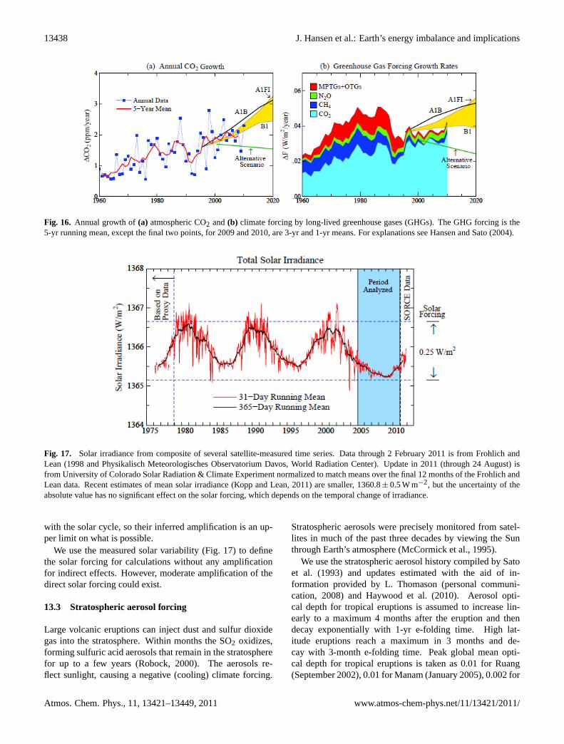
13438 J. Hansen et al.: Earth’s energy imbalance and implications
Fig. 15. Schematic diagram of Earth's energy imbalance (above) from Trenberth and Fasullo (2010) and (below) as calculated in this study. Our calculated imbalance, the top edge of the red area, is the moving 6-year trend of the calculated planetary energy imbalance for the intermediate response function. The red area is energy uptake by melting ice and warming ground and air. Measured ocean is 6-year trends of Argo analyses (see text) plus two small deep ocean terms from Purkey and Johnson (2010). Although the calculated decline of the energy imbalance is modest, it is significant because its origin in the solar irradiance minimum and Pinatubo volcanic aerosol rebound effect is insensitive to uncertainties in ocean mixing and climate sensitivity.
Fig.16. Annual growth of (a) atmospheric CO2 and (b) climate forcing by long-lived greenhouse gases (GHGs). The GHG forcing is the 5-year running mean, except the final two points, for 2009 and 2010, are 3-year and 1-year means. For explanations see Hansen and Sato (2004).
9
Fig. 16. Annual growth of(a) atmospheric CO2 and(b) climate forcing by long-lived greenhouse gases (GHGs). The GHG forcing is the5-yr running mean, except the final two points, for 2009 and 2010, are 3-yr and 1-yr means. For explanations see Hansen and Sato (2004).
Fig. 17. Solar irradiance from composite of several satellite-measured time series. Data through 2 February 2011 is from Frohlich and Lean (1998 and Physikalisch Meteorologisches Observatorium Davos, World Radiation Center). Update in 2011 (through 24 August) is from University of Colorado Solar Radiation & Climate Experiment normalized to match means over the final 12 months of the Frohlich and Lean data. Recent estimates of mean solar irradiance (Kopp and Lean, 2011) are smaller, 1360.8±0.5 W/m2, but the uncertainty of the absolute value has no significant effect on the solar forcing, which depends on the temporal change of irradiance.
10
Fig. 17. Solar irradiance from composite of several satellite-measured time series. Data through 2 February 2011 is from Frohlich andLean (1998 and Physikalisch Meteorologisches Observatorium Davos, World Radiation Center). Update in 2011 (through 24 August) isfrom University of Colorado Solar Radiation & Climate Experiment normalized to match means over the final 12 months of the Frohlich andLean data. Recent estimates of mean solar irradiance (Kopp and Lean, 2011) are smaller, 1360.8± 0.5 W m−2, but the uncertainty of theabsolute value has no significant effect on the solar forcing, which depends on the temporal change of irradiance.
with the solar cycle, so their inferred amplification is an up-per limit on what is possible.
We use the measured solar variability (Fig. 17) to definethe solar forcing for calculations without any amplificationfor indirect effects. However, moderate amplification of thedirect solar forcing could exist.
13.3 Stratospheric aerosol forcing
Large volcanic eruptions can inject dust and sulfur dioxidegas into the stratosphere. Within months the SO2 oxidizes,forming sulfuric acid aerosols that remain in the stratospherefor up to a few years (Robock, 2000). The aerosols re-flect sunlight, causing a negative (cooling) climate forcing.
Stratospheric aerosols were precisely monitored from satel-lites in much of the past three decades by viewing the Sunthrough Earth’s atmosphere (McCormick et al., 1995).
We use the stratospheric aerosol history compiled by Satoet al. (1993) and updates estimated with the aid of in-formation provided by L. Thomason (personal communi-cation, 2008) and Haywood et al. (2010). Aerosol opti-cal depth for tropical eruptions is assumed to increase lin-early to a maximum 4 months after the eruption and thendecay exponentially with 1-yr e-folding time. High lat-itude eruptions reach a maximum in 3 months and de-cay with 3-month e-folding time. Peak global mean opti-cal depth for tropical eruptions is taken as 0.01 for Ruang(September 2002), 0.01 for Manam (January 2005), 0.002 for
Atmos. Chem. Phys., 11, 13421–13449, 2011 www.atmos-chem-phys.net/11/13421/2011/

J. Hansen et al.: Earth’s energy imbalance and implications 13439
Soufriere (May 2006), 0.0023 for Kasatochi (August 2008),and 0.005 for Sarychev (June 2009). High latitude eruptions(Kasatochi and Sarychev) are assumed to cover only1/4 ofthe globe (30–90◦ N) The updated aerosol history is avail-able athttp://data.giss.nasa.gov/modelforce/strataer/The ef-fective forcing is taken as
F(τ) = −23τ, (4)
where τ is the global mean aerosol optical depth, as dis-cussed by Hansen et al. (2005b).
The ability of radiation calculations to simulate the effectof stratospheric aerosols on reflected solar and emitted ther-mal spectra was tested (Fig. 11 of Hansen et al., 2005) us-ing Earth’s measured radiation imbalance (Wong et al., 2005)following the 1991 Pinatubo eruption. Good agreement wasfound with the observed temporal response of solar and ther-mal radiation, but the observed net radiation change wasabout 25 percent smaller than calculated. Because of uncer-tainties in measured radiation anomalies and aerosol proper-ties, that difference is not large enough to define any changeto the stratospheric aerosol forcing. It is noteworthy that re-duction of volcanic aerosol forcing by that amount wouldbring simulated temperatures after historic eruptions intocloser agreement with observations (Robock, 2000; Hansenet al., 1996), but given the absence of further evidence weemploy the above equation for aerosol forcing.
An alternative stratospheric aerosol time series for re-cent decades has recently been suggested by Solomon etal. (2011). Their stratospheric aerosol optical depth issmaller than ours at times of some of the specific vol-canic eruptions listed above, but otherwise generally largerthan ours because of an inferred growing background strato-spheric aerosol amount. We repeated the computations ofSect. 13.4 using the aerosol optical depth from Fig. 2 ofSolomon et al. (2011). As expected, because the change ofaerosol optical depth is∼0.005, the effect of this alterna-tive stratospheric aerosol history is small and does not no-ticeably alter the calculated decadal energy imbalance or theinferred tropospheric aerosol optical depth, the latter beingmuch larger than the change of stratospheric aerosol opticaldepth.
13.4 Simulated surface temperature and energyimbalance
We examine the effect of each of the climate forcings onglobal mean temperature and planetary energy imbalance(Fig. 18). All cases use the intermediate climate responsefunction of Fig. 5, which yields the most realistic oceanheat storage. The combination of all forcings yields a de-cline in the planetary energy imbalance over the past decade(Fig. 18a). Here we will determine which specific forcingsare responsible for this decline of the energy imbalance.
GHGs (Fig. 18b) and tropospheric aerosols (Fig. 18c)are the principal forcings determining the trend of global
temperature in the past century. GHG plus troposphericaerosols (Fig. 18d) yields a flat planetary energy imbal-ance beginning a quarter century ago at a level of about0.6 W m−2, less than the maximum imbalance of about1 W m−2 due to all forcings. That flattening is a consequenceof the fact that the growth rate of the GHG forcing stopped in-creasing about 1980 and then declined to a lower level about1990 (Fig. 16b). The flat energy balance due to these princi-ple forcings allows small negative forcings in the past decadeand the Pinatubo eruption 20 yr ago to cause first a rise ofEarth’s energy imbalance and then a decline.
Volcanoes (Fig. 18e) cause a negative planetary energy im-balance during the 1–2 yr that the aerosols are present in thestratosphere, followed by a rebound to a positive planetaryenergy imbalance. This rebound is most clearly defined af-ter the Pinatubo eruption, being noticeable for more than adecade, because of the absence of other volcanoes in that pe-riod.
The physical origin of the rebound is simple. Solar heat-ing of Earth returns to its pre-volcano level as aerosols exitthe stratosphere. However, thermal emission to space is re-duced for a longer period because the ocean was cooled bythe volcanic aerosols. In calculations via the response func-tion, using Eq. (2), the volcanic aerosols introduce adF/dt
of one sign and within a few years adF/dt of opposite sign.The integrated (cumulative)dF/dt due to the volcano is zerobut the negativedF/dt occurred earlier, so its effect on tem-perature, defined by the climate response function, is greater.The effect of the temporal spacing between the negative andpositive changes ofF decreases as time advances subsequentto the eruption.
The planetary energy imbalance caused by solar irradiancevariability is in phase with the irradiance, but temperaturemaxima and minima lag irradiance maxima and minima by1–2 yr (Fig. 18g). The lag is due to the ocean’s thermal iner-tia, but the length of the lag incorporates, via the responsefunction, the effect of both the ocean and continental re-sponses to the forcing.
The reduction of planetary energy imbalance between2000 and 2009 due to declining solar irradiance is about0.14 W m−2. If there is an indirect effect magnifying thesolar forcing, the calculated effect on the planetary energyimbalance must be increased by that magnification factor.As discussed in Sect. 13.2, empirical correlations of the so-lar cycle and global temperature show that any magnificationcannot exceed a factor of two at most.
In summary, precipitous decline in the growth rate of GHGforcing about 25 yr ago caused a decrease in the rate ofgrowth of the total climate forcing and thus a flattening ofthe planetary energy imbalance over the past two decades.That flattening allows the small forcing due to the solar cycleminimum, a delayed bounceback effect from Pinatubo cool-ing, and recent small volcanoes to cause a decrease of theplanetary energy imbalance over the past decade.
www.atmos-chem-phys.net/11/13421/2011/ Atmos. Chem. Phys., 11, 13421–13449, 2011

13440 J. Hansen et al.: Earth’s energy imbalance and implications
Fig. 18. Climate forcings and their contributions (red curves) to temperature change and planetary energy imbalance. (a) shows the effect of the total forcing and (b) through (g) show effects of individual forcings. Observed global temperature change is included in the middle column for comparison; base period for temperature is 1951-1980 (zero mean) for observations and model.
11
Fig. 18. Climate forcings and their contributions (red curves) to temperature change and planetary energy imbalance.(a) shows the effectof the total forcing and(b) through(g) show effects of individual forcings. Observed global temperature change is included in the middlecolumn for comparison; base period for temperature is 1951–1980 (zero mean) for observations and model.
Atmos. Chem. Phys., 11, 13421–13449, 2011 www.atmos-chem-phys.net/11/13421/2011/
J. Hansen et al.: Earth’s energy imbalance and implications 13441
14 Discussion
Earth’s energy imbalance, averaged over several years, is afundamental characterization of the state of the climate. Itdetermines how much additional global temperature changeis “in the pipeline”. It defines how much current climate forc-ings must be altered to stabilize climate.
Earth’s average energy imbalance is expected to be only∼1 W m−2 or less (IPCC, 2007; Hansen et al., 2005a).Therefore assessment of the imbalance requires measure-ment accuracy approaching 0.1 W m−2. That target accuracyis just becoming conceivable, for data averaged over sev-eral years, with global distribution of Argo profiling floats.Measurements of Earth’s energy imbalance will be invalu-able for policy and scientific uses, if the observational sys-tem is maintained and enhanced. Implications of the data arediscussed here.
14.1 Human-made climate forcing versus solarvariability
Argo floats achieved good global distribution just in time fora valuable test of the effect of solar variability on Earth’s en-ergy imbalance and climate. The last half of the first decadeof the 21st century witnessed the deepest most prolonged so-lar minimum in the period of accurate solar monitoring thatbegan in the late 1970s (Fig. 17).
Earth’s energy imbalance during the solar minimum teststhe effect of solar variability on climate, including any am-plifications that may exist, such as the effect of cosmic rayson clouds. The imbalance during solar minimum is the neteffect of reduced solar irradiance and all other climate forc-ings, principally the net human-made climate forcing. Vol-canic aerosols added a small negative forcing (Fig. 18e) thatassisted the negative solar forcing.
Human-made forcing has been growing for more than acentury and thus has partially expended itself, causing mostof the 0.8◦C global warming of the past century. However,because of the ocean’s thermal inertia, the climate system hasonly partly responded to the human-made forcing. The por-tion of the human-made forcing that has not been respondedto constitutes a continuing forcing with positive sign (incom-ing energy exceeds outgoing energy). During the past 5–6 yrthe deep solar minimum caused a negative forcing6. Precisemeasurement of the planetary energy imbalance allows us to
6 Solar irradiance is negative in 2005–2010 relevant to the meanduring the period of measurements (Fig. 17). Recent solar forcing ispositive relevant to 1880 (Fig. 18g) in the scenario used by Hansenet al. (2007), which is based on Lean (2000). The reality of thesolar irradiance increase between 1900 and 1940, based on proxyindicators of solar activity, has been called into question by Leanet al. (2002). If the 1900-1940 solar irradiance increase is real, atleast half of its effect would already have been expended in globalwarming, thus leaving a small negative contribution to planetaryenergy imbalance in 2005–2010 (Fig. 18g).
determine whether the positive human-made forcing or neg-ative natural forcing is larger.
A verdict is provided by the ocean heat uptake foundby von Schuckmann and Le Traon (2011), 0.41 W m−2 for2005–2010, averaged over the planet7. Adding the smallterms for heat uptake in the deeper ocean, warming of theground and atmosphere, and melting of ice, the net plane-tary energy imbalance exceeded +0.5 W m−2 during the solarminimum.
The strong positive energy imbalance during the solar min-imum, and the consistency of the planet’s energy imbalancewith expectations based on estimated human-made climateforcing, together constitute a smoking gun, a fundamentalverification that human-made climate forcing is the dominantforcing driving global climate change. Positive net forcingeven during solar minimum assures that global warming willbe continuing on decadal time scales.
14.2 Climate response function
Earth’s climate response function, the fraction of global sur-face temperature response to a climate forcing as a functionof time, is a fundamental characteristic of the climate systemthat needs to be accurately determined. Climate models in-dicate that the response function has a characteristic shape,achieving almost half of its equilibrium response quickly,within about a decade. The remainder of the response is ex-ceedingly slow. We suggest, however, that this recalcitranceis exaggerated in many climate models.
GISS modelE-R, for example, achieves only 60 percentresponse in 100 yr. At least several other climate modelsused in IPCC (2001, 2007) studies have comparably slowresponse. Diagnostic studies of the GISS ocean model showthat it mixes too efficiently, which would cause its responsefunction to be too slow. Therefore we tested alternativeresponse functions that achieve 75 percent and 90 percentof their response after 100 yr. In each case we let currenthuman-made aerosol forcing have the magnitude that yieldsclosest agreement with observed global warming over thepast century.
The amount of energy pumped into the ocean by a pos-itive (warming) forcing depends on the response function,because this energy source (the planetary energy imbalance)shuts down as the surface temperature approaches its equi-librium response. Thus precise measurement of the rate ofocean heat uptake can help discriminate among alternativeresponse functions.
Ocean heat uptake during the Argo era agrees well withthe intermediate response function (75 percent response in100 yr) and is inconsistent with either the slow or fast re-sponse functions. We conclude that actual climate response
7 von Schuckmann and Le Traon (2011) find 0.54± 0.1 W m−2
for the top 1500 m of the ocean. Repeating their analysis for thetop 2000 m yields 0.59± 0.1 W m−2 (this paper), corresponding to0.41± 0.07 W m−2 globally.
www.atmos-chem-phys.net/11/13421/2011/ Atmos. Chem. Phys., 11, 13421–13449, 2011

13442 J. Hansen et al.: Earth’s energy imbalance and implications
is not as recalcitrant as many models suggest. As the Argorecord lengthens, and as issues about potential Argo biases(Barker et al., 2011) are resolved, knowledge of the realworld response function can be refined. The depth distri-bution of warming will be especially useful for confirmingthe nature of the climate response function, characterizing itsrecalcitrant response, and aiding development of ocean mod-els.
14.3 Aerosol climate forcing
Aerosol climate forcing is unmeasured. Aerosol uncertaintyis the principal barrier to quantitative understanding of on-going climate change. Until aerosol forcing is measured, itsmagnitude will continue to be crudely inferred, implicitly orexplicitly, via observations of climate change and knowledgeof climate sensitivity.
We explicitly allowed aerosol forcing and the climate re-sponse function to be free variables. We used observationsof global temperature change and ocean heat uptake to de-fine the aerosol forcing and response function that yield bestagreement with observations.
We assumed that aerosol forcing as a function of time hadthe shape of the aerosol curve in Fig. 1. Aerosol forcing for1880–1990, described by Hansen et al. (2007), is based onaerosol modeling (Koch, 2001) using aerosol emissions fromfuel use statistics and including temporal changes in fossilfuel technologies (Novakov et al., 2003). Our extension post-1990 assumed that aerosol forcing was half as large and op-posite in sign of the GHG forcing, as was the case in the priordecade. That crude assumption is consistent with moderatereduction of aerosol amount in developed countries and in-creasing aerosols in developing countries.
Our derived aerosol forcing in 2010 is−1.6 W m−2. Thisinferred aerosol forcing does not exceed IPCC (2007) a pri-ori estimated aerosol forcing including all indirect effects.More important, it is consistent with an insightful study ofEarth’s energy balance based on satellite measurements ofreflected solar radiation and emitted heat radiation (Murphyet al., 2009), as discussed in Sect. 14.6.
Our derived aerosol forcingdoesexceed aerosol forcingsemployed in most climate simulations carried out for IPCC(2001, 2007). For example, an ensemble of models from sev-eral groups (Fig. 9 of Stott and Forest, 2007) had aerosolforcings in the range−0.4 to−1.1 W m−2. Our interpreta-tion of why these models produced agreement with observedtemperature change over the past century is that the oceanmodels have a slow response function, slower than the realworld, mixing heat too efficiently into the deep ocean, and wehave cited several ocean model/data comparisons that pro-vide some support for this interpretation.
14.4 Implications for climate stabilization
Earth is out of energy balance by at least 0.5 W m−2. Ifother forcings are unchanged, atmospheric CO2 must be re-duced 30 ppm, to a level approximately 360 ppm, to increaseEarth’s heat radiation to space by 0.5 W m−2.
However, the measured energy imbalance was0.58 W m−2 in 2005–2010, during a deep solar mini-mum. We estimate the energy imbalance averaged over asolar cycle as∼0.75 W m−2. In that case, CO2 would needto be reduced to about 345 ppm to restore energy balance, ifother factors are fixed.
Other factors are not fixed, but CO2 is the dominant forc-ing of long-term climate. It should be practical to keep thenet effect of other human-made climate forcings close tozero, provided CO2 and global warming are limited. Poten-tial reduction of human-made climate forcing by CH4, CFCsand black soot can largely compensate for the increase inforcing that will occur as an expected decrease of human-made reflective aerosols occurs (Hansen et al., 2000; Ra-manathan et al., 2001; Jacobson, 2001). However, if CO2and global warming are not limited, release of CH4 via melt-ing of tundra and methane hydrates may frustrate attempts toprevent growth of non-CO2 forcings.
Thus a target CO2 level of 350 ppm (Hansen et al., 2008)is an appropriate initial goal for climate stabilization. Refine-ments can be made later, as the world approaches that goal.
Exact restoration of planetary energy balance is not nec-essarily the optimum target to achieve long-term climate sta-bilization. Global warming already in place may have unde-sirable effects via slow feedbacks, for example on ice sheetstability and sea level. Such issues must be evaluated, forexample via continued monitoring of ice sheet mass balance,as planetary energy balance is approached. A moderatelynegative planetary energy imbalance may be needed to stabi-lize sea level. Such refinements will become a practical issueonly after GHGs have been reduced to a level that approxi-mates planetary energy balance.
14.5 Implications for sea level
Sea level rise has averaged about 3 mm yr−1 since satellitemeasurements began in the early 1990s (Fig. 12). Thermalexpansion of ocean water and ice melt can account for sealevel rise of that magnitude. Assuming that the nearly con-stant rate of sea level rise in Fig. 12 is accurate, the nearconstancy is perhaps a consequence of an increasing rate ofice melt and decreasing thermal expansion. Annual thermalexpansion of the ocean is expected to have been maximum in1993 because ocean cooling due to the 1991 Pinatubo erup-tion would have peaked, leaving the gap between equilibriumand actual global temperature at a maximum. Although thereis large interannual variability associated with the El Nino/LaNina cycle, thermal expansion should have been on a down-ward trend from 1993 to the present. Ice melt, in contrast,
Atmos. Chem. Phys., 11, 13421–13449, 2011 www.atmos-chem-phys.net/11/13421/2011/

J. Hansen et al.: Earth’s energy imbalance and implications 13443
has probably been increasing over the period 1993–present(Fig. 8c).
Curiously, the rate of sea level rise seems to have slowed inthe past six years (2005–2010) to about 2 mm yr−1 (Fig. 12),despite the apparently increasing rate of mass loss from theGreenland and Antarctic ice sheets (Fig. 8c). This slowerrate of sea level rise appears to favor the lower estimates ofice melt. However, the slower rate of sea level rise during2005–2010 is probably due at least in part to the La Ninain 2009–2010. Although the effect of La Nina on the verti-cal distribution of temperature in the ocean (Roemmich andGilson, 2011) should be captured in the analysis of thermalexpansion based on Argo data, the water storage on conti-nents during La Nina as a consequence of heavy rainfall andfloods (Llovel et al., 2011) could account for much of thetemporary slowdown of sea level rise.
We conclude that the recent low (2 mm yr−1) rate of sealevel rise is unlikely to continue. This expectation is basednot only on the fact that the slowdown was partly a “weathernoise” effect of variability of the hydrologic cycle. In addi-tion we expect an increased rate of the background rate ofsea level rise during the next several years due to the inferredplanetary energy imbalance, the reasons being as follows.
First, the contribution of thermal expansion to sea levelis likely to increase above recent rates. Solar minimum anda diminishing Pinatubo rebound effect both contributed toa declining rate of thermal expansion during the past sev-eral years. But the Pinatubo effect is now essentially spentand solar irradiance change should now work in the oppositesense.
Second, the rate of ice melt is likely to continue to acceler-ate. Planetary energy imbalance now is positive, substantial,and likely to increase as greenhouse gases and solar irradi-ance increase. Thus, despite year-to-year fluctuations, globaltemperature will increase this decade and there will be a sub-stantial flux of energy into the ocean. Increasing ocean heatcontent provides energy for melting sea ice and ice shelves.Sea ice protects the ice sheets from heating and ice shelvesmechanically buttress the ice sheets. It has been argued thatloss of these protections of the surrounding ice may be themost important factor causing more rapid discharge from icesheets to the ocean (Hansen, 2005, 2007).
14.6 Implications for observations
Earth’s energy imbalance and its changes will determine thefuture of Earth’s climate. It is thus imperative to measureEarth’s energy imbalance and the factors that are changingit.
14.6.1 Measuring Earth’s energy imbalance
The required measurement accuracy is∼0.1 W m−2, in viewof the fact that estimated current (2005–2010) energy imbal-ance is 0.58 W m−2. The accuracy requirement refers to the
energy imbalance averaged over several years. It is this aver-age imbalance that drives future climate. Stabilization of cli-mate requires the energy imbalance averaged over El Nino-La Nina variability and the solar cycle to be close to zero.
There are two candidate measurement approaches:(1) satellites measuring the sunlight reflected by Earth andheat radiation to space, (2) measurements of changes in theheat content of the ocean and the smaller heat reservoirs onEarth. Each approach has problems. There is merit in pursu-ing both methods, because confidence in the result will be-come high only when they agree or at least the reasons thatthey differ are understood.
The difficulty with the satellite approach becomes clearby considering first the suggestion of measuring Earth’s re-flected sunlight and emitted heat from a satellite at the La-grange L1 point, which is a location between the Sun andEarth at which the gravitational pulls from these bodies areequal and opposite. From this location the satellite wouldcontinually stare at the sunlit half of Earth.
The notion that a single satellite at this point could mea-sure Earth’s energy imbalance to 0.1 W m−2 is prima faciepreposterous. Earth emits and scatters radiation in all di-rections, i.e., into 4π steradians. How can measurement ofradiation in a single direction provide a proxy for radiationin all directions? Climate change alters the angular distri-bution of scattered and emitted radiation. It is implausiblethat changes in the angular distribution of radiation could bemodeled to the needed accuracy, and the objective is to mea-sure the imbalance, not guess at it. There is also the difficultyof maintaining sensor calibrations to accuracy 0.1 W m−2,i.e., 0.04 percent. That accuracy is beyond the state-of-theart, even for short periods, and that accuracy would need tobe maintained for decades. There are many useful measure-ments that could be made from a mission to the Lagrange L1point, but Earth’s radiation balance in not one of them.
These same problems, the changing angular distribution ofthe scattered and emitted radiation fields and maintaining ex-treme precision of sensors over long periods, must be facedby Earth-orbiting satellites. Earth radiation budget satelliteshave progressed through several generations and improvedconsiderably over the past half-century, and they providevaluable data, e.g., helping to define energy transport fromlow to high latitudes. The angular distribution problem istreated via empirical angular distribution models, which areused to convert measurements of radiation in a given direc-tion into radiative (energy) fluxes.
The precision achieved by the most advanced generationof radiation budget satellites is indicated by the planetary en-ergy imbalance measured by the ongoing CERES (Cloudsand the Earth’s Radiant Energy System) instrument (Loeb etal., 2009), which finds a measured 5-yr-mean imbalance of6.5 W m−2 (Loeb et al., 2009). Because this result is implau-sible, instrumentation calibration factors were introduced toreduce the imbalance to the imbalance suggested by climatemodels, 0.85 W m−2 (Loeb et al., 2009).
www.atmos-chem-phys.net/11/13421/2011/ Atmos. Chem. Phys., 11, 13421–13449, 2011

13444 J. Hansen et al.: Earth’s energy imbalance and implications
The problems being addressed with this tuning probablyinvolve the high variability and changes of the angular distri-bution functions for outgoing radiation and the very limitedsampling of the radiation field that is possible from an orbit-ing satellite, as well as, perhaps, detector calibration. Therecan be no credible expectation that this tuning/calibrationprocedure can reduce the error by two orders of magnitudeas required to measure changes of Earth’s energy balance toan accuracy of 0.1 W m−2.
These difficulties do not imply that attempts to extractthe Earth’s radiation imbalance from satellite measurementsshould not be continued and improved as much as possi-ble. The data are already useful for many purposes, andtheir value will only increase via continued comparisons withother data such as ocean heat uptake.
An alternative potentially accurate approach to measureEarth’s energy imbalance is via changes in the ocean heatcontent, as has been argued for decades (Hansen et al.,1997) and as is now feasible with Argo data (Roemmich andGilson, 2009; Von Schuckmann and Le Traon, 2011). Thisapproach also has sampling and instrument calibration prob-lems, but it has a fundamental advantage: it is based on ab-solute measurements of ocean temperature. As a result, theaccuracy improves as the record length increases, and it isthe average energy imbalance over years and decades that isof greatest interest.
The error estimated by von Schuckmann and LeTraon (2011) for ocean heat uptake in the upper 2000 m ofthe ocean,±0.1 W m−2 for the ocean area or±0.07 W m−2
for the planetary energy imbalance, does not include an es-timate for any remaining systematic calibration errors thatmay exist. At least some such errors are likely to exist, asshown by Barker et al. (2011), so continuing efforts to testthe data and improve calibrations are needed. The Argo pro-gram needs to be continued and expanded to achieve furtherimprovement and minimization of error.
The Argo floats drift in location and have finite lifetime, soit is necessary to continually add about 800 floats per year tomaintain the system. Ocean south of 60◦ S (includes 5.6 per-cent of the ocean area) and north of 60◦ N (4.7 percent ofocean area) is not well sampled by Argo. Floats capableof operating under sea ice need to be deployed in the po-lar oceans, and floats capable of extending the measurementsinto the deep and abyssal oceans need to be developed. Thatmore spatially complete data would help define the nature ofthe climate response function, characterize the climate sys-tem’s recalcitrant response, and aid development of oceanmodels.
14.6.2 Measuring the cause of Earth’s energyimbalance
We also must quantify the causes of changes of Earth’s en-ergy imbalance. The two dominant causes are changes ofgreenhouse gases, which are measured very precisely, and
changes of atmospheric aerosols. It is remarkable and unten-able that the second largest forcing that drives global climatechange remains unmeasured. We refer to the direct and indi-rect effects of human-made aerosols.
We have inferred indirectly, from the planet’s energy im-balance and global temperature change, that aerosols areprobably causing a forcing of about−1.6 W m−2 in 2010.Our estimated uncertainty, necessarily partly subjective,is± 0.3 W m−2, thus a range of aerosol forcing from−1.3to −1.9 W m−2.
Our conclusion can be compared with an insightful anal-ysis of Murphy et al. (2009), which uses measurements ofocean heat content, greenhouse gases, volcanic aerosols, andcorrelations between surface temperature and satellite ra-diative flux measurements to infer a residual planetary en-ergy flux that they presume to be caused by aerosol directand indirect radiative forcing. Their result is an averageaerosol forcing of−1.1± 0.4 W m−2 for the period 1970–2000. For that period the aerosol forcing that we find (Fig. 1)is −1.2± 0.3 W m−2. The time dependence of the residualflux imbalance found by Murphy et al. (2009) is shown intheir Fig. 4c. It has an imbalance of about−1.5 W m−2 in2000 at the end of their analysis, which is consistent with ouranalysis.
These analyses tend to confirm that aerosol forcing is largeand negative, but cannot tell us what aerosols are causingthe forcing, how much of the forcing is due to indirect ef-fects on clouds, and how the aerosol forcing is changing.Aerosol climate forcing is complex (Ramanathan et al., 2001;Ramaswamy et al., 2001), in part because there are manydifferent aerosol compositions distributed inhomogeneouslyaround the planet. Different compositions have different ef-fects on solar radiation, and, via their effects on clouds, theyhave different effects on terrestrial thermal radiation.
Determination of the aerosol climate forcing requires mea-suring the aerosol physical properties and how those proper-ties are changing. This is analogous to how climate forcingby greenhouse gases is determined. We cannot determinethe greenhouse gas forcing by measuring the radiation withinthe atmosphere or from a satellite – there are too many fac-tors that affect the radiation field, including climate changes,cloud changes, etc. Instead we measure the changes of CO2,CFCs and other gases. We then compute, from basic physics,the climate forcing with an accuracy of better than 10 per-cent; even higher accuracy is possible, but not essential.
Existing satellite measurements provide an estimate ofaerosol optical depth (Mishchenko and Geogdzhayev, 2007;Mishchenko et al., 2007b), but maps of this quantity showdecreases and increases in various regions, some presumablydominated by reflecting sulfates, some by partially absorbingdust, some by weakly or heavily absorbing organic particlesor black soot. These existing measurements do not determineaerosol climate forcing and how it is changing.
It has been shown, from theory, aircraft observations, andplanetary studies (Mishchenko et al., 2007a) that as many
Atmos. Chem. Phys., 11, 13421–13449, 2011 www.atmos-chem-phys.net/11/13421/2011/

J. Hansen et al.: Earth’s energy imbalance and implications 13445
as 10 parameters defining aerosol properties can be obtainedusing satellite measurements that fully characterize reflectedsolar radiation. Full characterization requires: (1) measure-ment of the linear polarization of the reflected radiation toan accuracy of the order of 0.1 percent, (2) measurement atseveral spectral bands spanning reflected solar radiation fromthe near-ultraviolet to the near-infrared, (3) measurement ofthe radiation over the full range of scattering angles avail-able by scanning from horizon to horizon along the satelliteground track. Such measurements suffice to determine thedirect aerosol climate forcing.
Polarization measurements of reflected sunlight also yieldinformation about cloudtop droplets. However, determina-tion of the aerosol indirect climate forcing requires precisemeasurement of small changes in clouds induced by aerosolchanges. Cloud particles are one to two orders of magni-tude larger than aerosols and thus clouds can be characterizedbest via measurement of thermal emission at wavelengths 5–50 µm (200–2000 cm−1). The essential requirement is veryhigh wavelength-to-wavelength precision, because such highprecision data can yield atmospheric and cloud temperatures,cloud particle properties, and water vapor profile. The appro-priate instrument for achieving such precision is a Michel-son interferometer, because it records the signal from nearbywavelengths on the same detector.
The Glory mission (Mishchenko et al., 2007a), which wasexpected to begin operations this year, would have measuredthe aerosol direct forcing, as it carried an instrument capa-ble of measuring polarization to an accuracy about 0.1 per-cent. However, launch failure caused loss of the satellite,which failed to achieve orbit. A replacement mission is beingplanned with launch expected in the 2015–2016 time frame.Such detailed composition-specific global aerosol measure-ments will be essential to interpret changing planetary en-ergy balance. Presently the net effect of changing emissionsin developing and developed countries is highly uncertain.
The large aerosol forcing derived in our present study im-plies that the aerosol indirect climate forcing exceeds thedirect aerosol forcing, possibly by a large amount. Thereis no simple relationship between direct and indirect forc-ings, with each strongly dependent on aerosol composition.Understanding of the aerosol indirect forcing will require acombination of global observations, field measurements, anda range of modeling and analysis studies.
Global observations to determine the aerosol direct andindirect climate forcings will need to include simultaneousmeasurements of reflected solar and emitted thermal radia-tion fields as described above. The instruments measuringthese two radiation fields must look at the same area at es-sentially the same time. Such a mission concept has beendefined (Hansen et al., 1992) and recent reassessments indi-cate that it could be achieved at a cost of about $100 M ifcarried out by the private sector without a requirement forundue government review panels (B. Cairns, personal com-munication, 2011).
Acknowledgements.We thank two anonymous referees for manyhelpful suggestions, Gokhan Danabasoglu, Tom Delworth, andJonathan Gregory for providing data and papers defining responsesof the NCAR, GFDL and Hadley climate models, Greg Johnson,John Lyman and Sarah Purkey for providing ocean heat data andpreprints of their papers, Sarah Purkey for computing the sealevel rise due to Southern Ocean warming excluding overlap withArgo data, Catia Domingues for illuminating information, NormLoeb for references and discussion on satellite radiation budgetmeasurements, Eric Rignot for providing data on Greenland andAntarctic ice sheet mass balance, and Robert Gibson, WayneHamilton, John Marshall, Don McKensie, Gregory Monahan,Tim Palmer, Bill Rossow, Ken Schatten, Gavin Schmidt, SteveSchwartz and Michael Wright for comments on a draft of thispaper. Research support was provided by NASA managers JackKaye and David Considine, ClimateWorks, Lenfest Foundation,and the Rockefeller Family Fund. KvS work is partly supported bythe MyOcean FP7 project (European Commission).
Edited by: M. C. Facchini
References
Barker, P. M., Dunn, J. R., Domingues, C. M., and Wijffels, S.E.: Pressure sensor drifts in Argo and their impacts, J. Atmos.Oceanic Tech., in press,doi:10.1175/2011JTECHO831.1, 2011.
Barnett, T. P., Pierce, D. W., AchutaRao, K. M., Gleckler, P. J., San-ter, B. D., Gregory, J. M., and Washington, W. M.: Penetration ofhuman-induced warming into the world’s oceans, Science, 309,284–287, 2005.
Beltrami, H.: Climate from borehole data: Energy fluxes andtemperatures since 1500, Geophys. Res. Lett., 29, 2111,doi:10.1029/2002GL015702, 2002.
Beltrami, H., Smerdon, J. E., Pollack, H. N., and Huang, S.: Con-tinental heat gain in the global climate system, Geophys. Res.Lett., 29, 1167,doi:10.1029/2001GL014310, 2002.
Bleck, R.: An oceanic general circulation model framed in hybridisopycnic-Cartesian coordinates, Ocean Model., 4, 55–88, 2002.
Bromwich, D. H. and Nicolas, J. P.: Ice-sheet uncertainty, Nat.Geosci., 3, 596–597, 2010.
Bryan, K.: A numerical model for the study of the circulation of theworld ocean, J. Comp. Phys., 3, 347–376, 1969.
Calgovic, J., Albert, C., Arnold, F., Beer, J., Desorgher, L.,and Fluedkiger, E. O.: Sudden cosmic ray decreases: Nochange of global cloud cover, Geophys. Res. Lett., 37, L03802,doi:10.1029/2009GL041327, 2010.
Canuto, V. M. Howard, A. M., Cheng, Y., Muller, C. J.,Leboissetier, A., Jayne, S. R. : Ocean turbulence, III: NewGISS vertical mixing scheme, Ocean Model., 34, 70–91,doi:10.1038/nature07080, 2010.
Charney, J. G., Arakawa, A., Baker, D., Bolin, B., Dickenson, R.,Goody, R., Leith, C., Stommel, H., and Wunsch, C.: CarbonDioxide and Climate: A Scientific Assessment, Natl. Acad. Sci.Press, Washington DC, USA, 33 pp., 1979.
Cox, M. D.: A primitive equation, three dimensional model of theocean, GFDL Ocean Group Tech. Rep. 1, Princeton NJ, USA,143 pp. 1984.
Delworth, T. L., Stouffer, R. J., Dixon, K. W., Spelman, M. J., Knut-son, T. R., Broccoli, A. J., Kushner, P. J., and Wetherald, R. T.:
www.atmos-chem-phys.net/11/13421/2011/ Atmos. Chem. Phys., 11, 13421–13449, 2011

13446 J. Hansen et al.: Earth’s energy imbalance and implications
Review of simulations of climate variability and change with theGFDL R30 coupled climate model, Clim. Dynam., 19, 555–574,2002.
Domingues, C. M., Church, J. A., White, N. J., Gleckler, P. J., Wijf-fels, S. E., Barker, P. M., and Dunn, J. R.: Improved estimates ofupper-ocean warming and multi-decadal sea-level rise, Nature,453, 1090–1093,doi:10.1038/nature/07080, 2008.
Forest, C. E., Stone, P. H., and Sokolov, A. P.: EstimatedPDFs of climate system properties including natural andanthropogenic forcings, Geophys. Res. Lett., 33, L01705,doi:10.1029/2005GL023977, 2006.
Frohlich, C. and Lean, J.: The Sun’s total irradiance: Cycles andtrends in the past two decades and associated climate change un-certainties, Geophys. Res. Lett., 25, 4377–4380, 1998.
Gordon, C., Cooper, C., Senior, C. A., Banks, H., Gregory, J. M.,Johns, T. C., Mitchell, J. F. B., and Wood, R. A.: The simulationof SST, sea ice extents and ocean heat transports in a versionof the Hadley Centre coupled model without flux adjustments,Clim. Dynam., 16, 147–168, 2000.
Gregory, J. M., Ingram, W. J., Palmer, M. A., Jones, G. S.,Stott, P. A., Thorpe, R. B., Lowe, J. A., Johns, T. C., andWilliams, K. D.: A new method for diagnosing radiative forc-ing and climate sensitivity, Geophys. Res. Lett., 31, L03205,doi:10.1029/2003GL018747, 2004.
Griffies, S. M., Biastoch, A., Boning, C., Bryan, F., Danabasoglu,G., Chassignet, E. P., England, M. H., Gerdes, R., Haak, H., Hall-berg, R. W., Hazeleger, W., Jungclaus, J., Large, W. G., Madec,G., Pirani, A., Samuels, B. L., Scheinert, M., Gupta, A. S., Sev-erijns, C. A., Simmons, H. L., Treguier, A. M., Winton, M., Yea-ger, S., and Yin, J.: Coordinated ocean-ice reference experiments(COREs), Ocean Model., 26, 1–46, 2009.
Hansen, J.: Climate threat to the planet: implications for energypolicy and intergenerational justice, Bjerknes lecture, AmericanGeophysical Union, San Francisco, 17 December, available at:http://www.columbia.edu/∼jeh1/presentations.shtml, 2008.
Hansen, J.: Storms of My Grandchildren: The Truth about the Com-ing Climate Catastrophe and Our Last Chance to Save Humanity,Bloomsbury, 304 pp., 2009.
Hansen, J. and Sato, M.: Greenhouse gas growth rates, Proc. Natl.Acad. Sci., 101, 16109–16114, 2004.
Hansen, J. and Sato M.: Paleoclimate implications for human-madeclimate change in Climate Change: Inferences from Paleoclimateand Regional Aspects, edited by: Berger, A., Mesinger, F., andSijacki, D., Springer, in press, 350 pp., 2012.
Hansen, J., Russell, G., Lacis, A., Fung, I., Rind, D., and Stone, P.:Climate response times: dependence on climate sensitivity andocean mixing, Science, 229, 857–859, 1985.
Hansen, J., Rossow, W., and Fung, I.: Long-term Monitoring ofGlobal Climate Frocings and Feedbacks, NASA Conf. Publ.3234, Goddard Institute for Space Studies, New York, USA,1992.
Hansen, J., Sato, M., Ruedy, R., Lacis, A., Asamoah, K., Boren-stein, S., Brown, E., Cairns, B., Caliri, G., Campbell, M., Cur-ran, B., de Castro, S., Druyan, L., Fox, M., Johnson, C., Lerner,J., McCormick, M. P., Miller, R. L., Minnis, P., Morrison, A.,Pandolfo, L., Ramberran, I., Zaucker, F., Robinson, M., Russell,P., Shah, K., Stone, P., Tegen, I., Thomason, L., Wilder, J., andWilson, H.: A Pinatubo climate modeling investigation, in: TheMount Pinatubo Eruption: Effects on the Atmosphere and Cli-
mate, NATO ASI Series, Vol. I 42, edited by: Fiocco, G., Fua,D., and Visconti, G., Springer-Verlag, 233–272, 1996.
Hansen, J., Sato, M., Ruedy, R., Lacis, A., Asamoah, K., Beckford,K., Borenstein, S., Brown, E., Cairns, B., Carlson, B., Curran,B., de Castro, S., Druyan, L., Etwarrow, P., Ferede, T., Fox, M.,Gaffen, D., Glascoe, J., Gordon, H., Hollandsworth, S., Jiang,X., Johnson, C., Lawrence, N., Lean, J., Lerner, J., Lo, K., Lo-gan, J., Luckett, A., McCormick, M. P., McPeters, R., Miller, R.L., Minnis, P., Ramberran, I., Russell, G., Russell, P., Stone, P.,Tegen, I., Thomas, S., Thomason, L., Thompson, A., Wilder, J.,Willson, R., and Zawodny, J.: Forcings and chaos in interannualto decadal climate change, J. Geophys. Res., 102, 25679–25720,1997.
Hansen, J., Sato, M., Ruedy, R., Lacis, A., and Oinas, V.: Globalwarming in the twenty-first century: An alternative scenario,Proc. Natl. Acad. Sci. USA, 97, 9875–9880, 2000.
Hansen, J., Nazarenko, L., Ruedy, R., Sato, M., Willis, J., Del Ge-nio, A., Koch, D., Lacis, A., Lo, K., Menon, S., Novakov, T.,Perlwitz, J., Russell, G., Schmidt, G. A., and Tausnev, N.: Earth’senergy imbalance: Confirmation and implications, Science, 308,1431–1435,doi:10.1126/science.1110252, 2005a.
Hansen, J., Sato, M., Ruedy, R., Nazarenko, L., Lacis, A., Schmidt,G. A., Russell, G., Aleinov, I., Bauer, M., Bauer, S., Bell, N.,Cairns, B., Canuto, V., Chandler, M., Cheng, Y., Del Genio, A.,Faluvegi, G., Fleming, E., Friend, A., Hall, T., Jackman, C., Kel-ley, M., Kiang, N. Y., Koch, D., Lean, J., Lerner, J., Lo, K.,Menon, S., Miller, R. L., Minnis, P., Novakov, T., Oinas, V.,Perlwitz, J. P., Perlwitz, J., Rind, D., Romanou, A., Shindell, D.,Stone, P., Sun, S., Tausnev, N., Thresher, D., Wielicki, B., Wong,T., Yao, M., and Zhang, S.: Efficacy of climate forcings, J. Geo-phys. Res., 110, D18104,doi:10.1029/2005JD005776, 2005b.
Hansen, J., Sato, M., Ruedy, R., Kharecha, P., Lacis, A., Miller, R.L., Nazarenko, L., Lo, K., Schmidt, G. A., Russell, G., Aleinov,I., Bauer, S., Baum, E., Cairns, B., Canuto, V., Chandler, M.,Cheng, Y., Cohen, A., Del Genio, A., Faluvegi, G., Fleming, E.,Friend, A., Hall, T., Jackman, C., Jonas, J., Kelley, M., Kiang,N. Y., Koch, D., Labow, G., Lerner, J., Menon, S., Novakov,T., Oinas, V., Perlwitz, J. P., Perlwitz, J., Rind, D., Romanou,A., Schmunk, R., Shindell, D., Stone, P., Sun, S., Streets, D.,Tausnev, N., Thresher, D., Unger, N., Yao, M., and Zhang, S.:Climate simulations for 1880–2003 with GISS modelE, Clim.Dynam., 29, 661–696,doi:10.1007/s00382-007-0255-8, 2007.
Hansen, J., Sato, M., Kharecha, P., Beerling, D., Berner, R.,Masson-Delmotte, V., Pagani, M., Raymo, M., Royer, D. L., andZachos, J. C.: Target atmospheric CO2: where should humanityaim? Open Atmos. Sci. J., 2, 217–231, 2008.
Hansen, J., Ruedy, R., Sato, M., and Lo, K.: Globalsurface temperature change, Rev. Geophys., 48, RG4004,doi:10.1029/2010RG000345, 2010.
Hansen, J. E.: A slippery slope: How much global warming consti-tutes “dangerous anthropogenic interference”? An editorial es-say, Climatic Change, 68, 269–279, 2005.
Hansen, J. E.: Scientific reticence and sea level rise, Environ. Res.Lett., 2, 024002,doi:10.1088/1748-9326/2/2/024002, 2007.
Hansen, J. E. and Lacis, A. A.: Sun and dust versus greenhousegases: An assessment of their relative roles in global climatechange, Nature, 346, 713–719,doi:10.1038/346713a0, 1990.
Harrison, D. E. and Carson, M.: Is the World Ocean warm-ing? Upper-ocean temperature trends: 1950–2000, J. Phys.
Atmos. Chem. Phys., 11, 13421–13449, 2011 www.atmos-chem-phys.net/11/13421/2011/

J. Hansen et al.: Earth’s energy imbalance and implications 13447
Oceanogr., 37, 174–187, 2007.Haywood, J. M., Jones, A., Clarisse, L., Bourassa, A., Barnes,
J., Telford, P., Bellouin, N., Boucher, O., Agnew, P., Clerbaux,C., Coheur, P., Degenstein, D., and Braesicke, P.: Observationsof the eruption of the Sarychev volcano and simulations usingthe HadGEM2 climate model, J. Geophys. Res. 115, D21212,doi:10.1029/2010JD014447, 2010.
Held, I. M., Winton, M., Takahashi, K., Delworth, T., Zeng, F., andVallis, G. K.: Probing the fast and slow components of globalwarming b returning abruptly to preindustrial forcing, J. Climate,23, 2418–2427, 2010.
Huang, S.: 1851–2004 annual heat budget of the con-tinental landmass, Geophys. Res. Lett., 33, L04707,doi:10.1029/2005GL025300, 2006.
Intergovernmental Panel on Climate Change (IPCC), ClimateChange 2001: The Scientific Basis, edited by: Houghton, J.T., Ding, Y., Griggs, D. J., Noguer, M., van der Linden, P. J.,Dai, X., Maskell, K., and Johnson, C. A., Cambridge UniversityPress, UK, 881 pp., 2001.
Intergovernmental Panel on Climate Change (IPCC), ClimateChange 2007: The Physical OlScience Basis, Solomon, S., Dahe,Q., Manning, M., Chen, Z., Marquis, M., Averyt, K. B.,Tignor,M., and Miller, H. L.: Cambridge Univ. Press, 996 pp., 2007.
Jacobson, M. Z.: Global direct radiative forcing due to multicompo-nent anthropogenic and natural aerosols, J. Geophys. Res., 106,1551–1568, 2001.
Kiehl, J. T., Shields, C. A., Hack, J. J., and Collins, W. D.: The cli-mate sensitivity of the Community Climate System Model ver-sion 3 (CCSM3), J. Climate, 19, 2584–2596, 2006.
Kirkby, J., Curtius, J., Almeida, J., Dunne, E., Duplissy, J., Ehrhart,S., Franchin, A., Gagne, S., Ickes, L., Kuurten, A., Kupc,A., Metzger, A., Riccobono, F., Rondo, L., Schobesberger, S.,Tsagkogeorgas, G., Wimmer, D., Amorim, A., Bianchi, F., Bre-itenlechner, M., David, A., Dommen, J., Downard, A., Ehn, M.,Flagan, R. C., Haider, S., Hansel, A., Hauser, D., Jud, W., Junni-nen, H., Kreissl, F., Kvashin, A., Laaksonen, A., Lehtipalo, K.,Lima, J., Lovejoy, E. R., Makhmutov, V., Mathot, S., Mikkila, J.,Minginette, P., Mogo S., Nieminen, T., Onnela, A., Pereira, P.,Petaja, T., Schnitzhofer, R., J. H. Seinfeld, Sipila, M., Stozhkov,Y., Stratmann, F., Tome, A., Vanhanen, J., Viisanen, Y., Vrtala,A., Wagner, P. E., Walther, H., Weingartner, E., Wex, H., Win-kler, P. M., Carslaw, K. S., Worsnop, D. R., Baltensperger, U.,and Kulmala, M.: Role of sulphuric acid, ammonia and galac-tic cosmic rays in atmospheric aerosol nucleation, Nature, 476,429–433, 2011.
Knutti, R.: Why are climate models reproducing the observedglobal surface warming so well?, Geophys. Res. Lett., 35,L18704,doi:10.1029/2008GL034932, 2008.
Koch, D.: Transport and direct radiative forcing of carbonaceousand sulfate aerosols in the GISS GCM, J. Geophys. Res., 106,20311–20332, 2001.
Kopp, G. and Lean, J. L.: A new, lower value of total solar irradi-ance: evidence and climate significance, Geophys. Res. Lett., 38,L01706,doi:10.1029/2010GL045777, 2011.
Kulmala, M., Riipinen, I., Nieminen, T., Hulkkonen, M., So-gacheva, L., Manninen, H. E., Paasonen, P., Petaja, T., Dal Maso,M., Aalto, P. P., Viljanen, A., Usoskin, I., Vainio, R., Mirme, S.,Mirme, A., Minikin, A., Petzold, A., Horrak, U., Pla-Dulmer,C., Birmili, W., and Kerminen, V.-M.: Atmospheric data over
a solar cycle: no connection between galactic cosmic rays andnew particle formation, Atmos. Chem. Phys., 10, 1885–1898,doi:10.5194/acp-10-1885-2010, 2010.
Leuliette, E. W. and Miller, L.: Closing the sea level budget withaltimetry, Argo, and GRACE, Geophys. Res. Lett., 36, L04608,doi:10.1029/2008GL036010, 2009.
Levitus, S. and Boyer, T. P.: Temperature, World Ocean Atlas 1994,Temperature, 4, NOAA Atlas NESDIS 3, 99 pp., 1994.
Levitus, S., Antonov, J. I., Boyer, T. P., and Stephens, C.: Warmingof the world ocean, Science, 287, 225–2229, 2000.
Levitus, S., Antonev, J. I., Wang, J., Delworth, T. L., Dixon, K. W.,and Broccoli, A. J.: Anthropogenic warming of earth’s climatesystem, Science, 292, 267–270, 2001.
Levitus, S., Antonov, J., and Boyer, T.: Warming ofthe world ocean, Geophys. Res. Lett., 32, L02604,doi:10.1029/2004GL021592, 2005.
Levitus, S., Antonov, J., Boyer, T., Locarnini, R. A., Garcia, H.E., and Mishonov, A. V.: Global ocean heat content 1955–2008in light of recently revealed instrumentation problems, Geo-phys. Res. Lett., 36, L07608,doi:10.1029/2008GL037155,http://www.nodc.noaa.gov/OC5/3MHEAT CONTENT/basindata.html, 1955–2010, 2009.
Loeb, N. G., Wielicki, B. A., Doelling, D. R., Smith, G. L., Keyes,D. F., Kato, S., Manalo-Smith, N., and Wong, T.: Toward opti-mal closure of the Earth’s top-of-atmosphere radiation budget, J.Climate, 22, 748–766, 2009.
Lyman, J. M.: Estimating Global Energy Flow from the GlobalUpper Ocean, Surv. Geophys.,doi:10.1007/s10712-011-9167-6,2011.
Lyman, J. M. and Johnson, G. C.: Estimating annual global upper-ocean heat content anomalies despite irregular in situ ocean sam-pling, J. Climate, 21, 5629–5641, 2008.
Lyman, J. M., Willis, J. K., and Johnson, G. C.: Recent cool-ing in the upper ocean, Geophys. Res. Ltt., 33, L18604,doi:10.1029/2006GL027033, 2006.
Lyman, J. M., Good, S. A., Gouretski, V. V., Ishii, M., Johnson,G. C., Palmer, M. D., Smith, D. A., and Willis, J. K.,: Ro-bust warming of the global upper ocean, Nature, 465, 334–337,doi:10.1038/nature09043, 2010.
McCormick, M. P., Thomason, L. W., and Trepte, C. R.: Atmo-spheric effects of Mt. Pinatubo eruption, Nature, 373, 399–404,1995.
Meier, M. F., Dyurgerov, M. B., Rick, U. K., O’Neel, S., Pfeffer,W. T., Anderson, R. S., Anderrson, S. P., and Glazovsky, A. F.:Glaciers dominate eustatic sea-level rise in the 21st century, Sci-ence, 317, 1064–1067, 2007.
Mishchenko, M. I. and Geogdzhayev, I. V.: Satellite remote sensingreveals regional tropospheric aerosol trends, Opt. Express, 15,7423–7438,doi:10.1364/OE.15.007423, 2007.
Mishchenko, M. I., Cairns, B., Kopp, G., Schueler, C. F., Fafaul,B. A., Hansen, J. E., Hooker, R. J., Itchkawich, T., Maring, H.B., and Travis, L. D.: Accurate monitoring of terrestrial aerosolsand total solar irradiance: Introducing the Glory mission, Bull.Amer. Meteorol. Soc., 88, 677–691,doi:10.1175/BAMS-88-5-677, 2007a.
Mishchenko, M. I., Geogdzhayev, I. V., Rossow, W. B., Cairns, B.,Carlson, B. E., Lacis, A. A., Liu, L., and Travis, L. D.: Long-term satellite record reveals likely recent aerosol trend, Science,315, 1543,doi:10.1126/science.1136709, 2007b.
www.atmos-chem-phys.net/11/13421/2011/ Atmos. Chem. Phys., 11, 13421–13449, 2011

13448 J. Hansen et al.: Earth’s energy imbalance and implications
Milly, P. C. C., Cazenave, A., Famiglietti, J. S., Gornitz, V., Laval,K., Lettenmaier, D. P., Sahagian, D. L., Wahr, J. M., and Wil-son, C. R.: Terrestrial water-storage contributions to sea-levelrise and variability, in: Understanding Sea-Level Rise and Vari-ability, edited by: Church, J. A., Woodworth, P. L., Aarup, T.and Wilson, W. S., Wiley Blackwell, Wiley Blackwell, 226–255,2010.
Munk, W.: Twentieth century sea level: an enigma, Proc. Natl.Acad. Sci., 99, 6550–6555, 2002.
Munk, W.: Ocean Freshening, Sea Level Rising, Science, 300,2041–2043, 2003.
Murphy, D. M., Solomon, S., Portmann, R. W., Rosenlof, K. H.,Forster, P. M., and Wong, T.: An observationally based energybalance for the Earth since 1950, J. Geophys. Res., 114, D17107,doi:10.1029/2009JD012105, 2009.
Nerem, R. S., Leuliette. E., and Cazenace A.: Present-day sea-levelchange: A review, C. R. Geoscience, 338, 1077–1083, 2006.
Novakov, T., Ramanathan, V., Hansen, J. E., Kirschstetter, T. W.,Sato, M., Sinton, J. E., and Sathaye, J. A.: Large historicalchanges of fossil-fuel black carbon aerosols, Geophys. Res. Lett.,30, 1324,doi:10.1029/2002GL016345, 2003.
Pacanowski, R., Dixon, K., and Rosati, A.: The GFDL ModularOcean Model users guide version 1, GFDL Ocean Group Tech.Rep. 2, 44 pp., Available from NOAA/Geophysical Fluid Dy-namics Laboratory, Princeton University, Rt. 1, Forrestal Cam-pus, Princeton NJ 08542, 1991.
Pierce, D. W., Barnett, T. P., AchutaRao, K. N., Gleckler, P. J., Gre-gory, J. M., and Washington, W. M.: Anthropogenic warmingof the oceans: observations and model results, J. Climate, 19,1873–1900, 2006.
Pope, V. D., Gallani, M. L., Rowntree, P. R., and Stratton, R. A.,:The impact of new physical parameterizations in the Hadley Cen-tre climate model – HadAM3, Clim. Dynam., 16, 123–146, 2000.
Purkey, S. G. and Johnson, G. C.: Warming of global abyssal anddeep southern ocean between the 1990s and 2000s: contributionsto global heat and sea level rise budgets, J. Climate, 23, 6336–6351, 2010.
Rahmstorf, S., Cazenave, A., Church, J. A., Hansen, J. E., Keeling,R. F., Parker, D. E., and Somerville, R. C. J.: Recent climate ob-servations compared to projections, Science, 316, p. 709, 2007.
Ramanathan, V., Crutzen, P. J., Kiehl, J. T., and Rosenfeld, D.:Aerosols, climate, and the hydrological cycle, Science, 294,2119–2124, 2001.
Ramaswamy, V., Boucher, O., Haigh, J., Hauglustaine, D., Hay-wood, J., Myhre, G., Nakajima, T., Shi, G. Y., and Solomon, S.:Radiative forcing of climate change, in: Climate Change 2001:The scientific basis, edited by: Houghton, J. T., Ding, Y., Griggs,D. J., Noguer, M., van der Linden, P. J., Dai, X., Maskell, K., andJohnson, C. A., Cambridge University Press, 349–416, 2001.
Randall, D. A., Wood, R. A., Bony, S., Colman, R., Fichefet, T.,Fyfe, J., Kattsov, V., Pitman, A., Shukla, J., Srinivasan, J., Stouf-fer, R. J., Sumi, A., and Taylor, K. E.: Climate Models and TheirEvaluation, in: Climate Change 2007: The Physical ScienceBasis. Contribution of Working Group I to the Fourth Assess-ment Report of the Intergovernmental Panel on Climate Change,edited by: Solomon, S., Qin, D., Manning, M., Chen, Z., Mar-quis, M., Averyt, K. B., Tignor, M., and Miller, H. L., CambridgeUniversity Press, Cambridge, United Kingdom and New York,NY, USA, 2007.
Rignot, E., Velicogna, I., van den Brooke, M. R., Monaghan, A.,and Lenarts, J. T. M.: Acceleration of the contribution of theGreenland and Antarctic ice sheets to sea level rise, Geophys.Res. Lett., 38, L05503,doi:10.1029/2011GL046583, 2011.
Robock, A.: Volcanic eruptions and climate, Rev. Geophys., 38,191–219, 2000.
Roemmich, D. and Gilson, J.: The 2004–2008 mean and annual cy-cle of temperature, salinity, and steric height in the global oceanfrom the Argo Program, Prog. Oceanogr., 82, 81–100, 2009.
Rothrock, D. A., Percival, D. B., and Wensnahan, M.: The declinein arctic sea-ice thickness: separating the spatial, annual, andinterannual variability in a quarter century of submarine data, J.Geophys. Res., 113, C05003,doi:10.1029/2007JC004252, 2008.
Russell, G. L., Miller, J. R., and Rind, D.: A coupled atmosphere-ocean model for transient climate change studies. Atmos.-Ocean,33, 683–730, 1995.
Sato, M., Hansen, J. E., McCormick, M. P., and Pollack, J. B.:Stratospheric aerosol optical depths, 1850–1990, J. Geophys.Res., 98, 22987–22994,doi:10.1029/93JD02553, 1993.
Schmidt, G. A., Ruedy, R., Hansen, J. E., Aleinov, I., Bell, N.,Bauer, M., Bauer, S., Cairns, B., Canuto, V., Cheng, Y., Del Ge-nio, A., Faluvegi, G., Friend, A. D., Hall, T. M., Hu, Y., Kelley,M., Kiang, N. Y., Koch, D., Lacis, A. A., Lerner, J., Lo, K. K.,Miller, R. L., Nazarenko, L., Oinas, V., Perlwitz, J. P., Perlwitz,J., Rind, D., Romanou, A., Russell, G. L., Sato, M., Shindell, D.T., Stone, P. H., Sun, S., Tausnev, N., Thresher, D., and Yao, M.-S.: Present day atmospheric simulations using GISS ModelE:comparison to in-situ, satellite and reanalysis data, J. Climate,19, 153–192, 2006.
Schmittner, A., Urban, N. M., Shakun, J. D., Mahowald,N. M., Clark, P. U., Bartllein, P. J., Mix, A. C., andRosell-Mele, A.: Climate sensitivity extimated from temper-ature reconstructions of the last glacial maximum, availableat: Scinceexpress/www.scienceexpress.org/24November2011/10.1126/science.1203513, 2011.
Shepherd, A., Wingham, D., Wallis, D., Giles, K., Laxon, S.,Sundal, A. V.: Recent loss of floating ice and the conse-quent sea level contribution, Geophys. Res. Lett., 37, L13503,doi:10.1029/2010GL042496, 2010.
Shindell, D., Schmidt, G. A., Miller, R. L., and Rind, D.: North-ern Hemisphere winter climate response to greenhouse gas, vol-canic, ozone and solar forcing, J. Geophys. Res., 106, 7193–7210, 2001.
Solomon, S., Daniel, J. S., Neely, R. R., Vernier, J. P., Dutton, E. G.,and Thomason, L. W.: The persistently variable “background”stratospheric aerosol layer and global climate change, Science,333, 866–870, 2011.
Sorensen, L. S. and Forsberg, R.: Greenland ice sheet mass lossfrom GRACE monthly models, in: Gravity, Geoid and EarthObservations, edited by: Mertikas, S. P., Iag. Symp., 135,doi:10.1007/978-3-10634-770, 2010.
Stott, P. A. and Forest, C. E.: Ensemble climate predictions us-ing climate models and observational constraints, Phil. Trans. R.Soc. A, 365, 2029–2052, 2007.
Svensmark, H., Bondo, T., and Svensmark, J.: Cosmic ray de-creases affect atmospheric aerosols and clouds, Geophys. Lett.,36, L15101,doi:10.1029/2009GL038429, 2009.
Trenberth, K. E.: An imperative for climate change planning: track-ing Earth’s global energy, Curr. Opin. Environ. Sustainability, 1,
Atmos. Chem. Phys., 11, 13421–13449, 2011 www.atmos-chem-phys.net/11/13421/2011/
J. Hansen et al.: Earth’s energy imbalance and implications 13449
19–27, 2009.Trenberth, K. E.: The ocean is warming, isn’t it?, Nature, 465, 304,
2010.Trenberth, K. E. and Fasullo, J. T.: Tracking Earth’s energy, Sci-
ence, 328, 316–317, 2010.Tung, K. K., Zhou, J., and Camp, C. D.: Constraining model tran-
sient climate response using independent observations of solar-cycle forcing and response, Geophys. Res. Lett., 35, L17707,doi:10.1029/2008GL034240, 2008.
Velicogna, I.: Increasing rates of ice mass loss from the Green-land and Antarctic ice sheets revealed by GRACE, Geophys. Res.Lett., 36, L19503,doi:10.1029/2009GL040222, 2009.
von Schuckmann, K. and Le Traon, P.-Y.: How well can we deriveGlobal Ocean Indicators from Argo data?, Ocean Sci., 7, 783–791,doi:10.5194/os-7-783-2011, 2011.
von Schuckmann, K., Gaillard, F., and Le Traon, P. Y.: Global hy-drographic variability patterns during 2003–2008, J. Geophys.Res., 114, C09007,doi:10.1029/2008JC005237, 2009.
Washington, W. M., Weatherly, J. W., Meehl, G. A., Semtner, A.J., Bettge, T. W., Craig, A. P., Strand, W. G., Arblaster, J., Way-land, V. B., James, R., and Zhang, Y.: Parallel climate mmodel(PCM) control and transient simulations, Clim. Dyn., 16, 755–774, 2000.
White, W. B., Lean, J., Cayan, D. R., and Dettinger, M. D.: Re-sponse of global upper ocean temperature to changing solar irra-diance, J. Geophys. Res., 102, 3255–3266, 1997.
White, W. B., Cayan, D. R., and Lean, J.: Global upper ocean heatstorage response to radiative forcing from changing solar irra-diance and increasing greenhouse gas/aerosol concentrations, J.Geophys. Res., 103, 21355–21366, 1998.
Whittington, A. G., Hofmeister, A. M., and Nabelek, P. I.:Temperature-dependent thermal diffusivity of the Earth’s crustand implications for magmatism, Nature, 458, 319–321,doi:10.1038/nature07818, 2009.
Wijffels, S. E., Willis, J., Domingues, C. M., Barker, P., White,N. J., Gronell, A., Ridgway, K., and Church, J. A.: Changing ex-pendable bathythermograph fall rates and their impact on estimesof thermosteric sea level rise, J. Clim., 21, 5657–5672, 2008.
Willis, J. K., Lyman, J. M., Johnson, G. C., and Gilson, J.: Correc-tion to “Recent cooling of the upper ocean”, Geophys. Res. Lett.,34, L16601,doi:10.1029/2007GL030323, 2007.
Winton, M., Takahashi, K., and Held, I. M.: Importance of oceanheat uptake efficiency to transient climate change, J. Climate, 23,2333–2344, 2010.
Wong, T., Wielicki, B. A., Lee, R. B., Smith, G. L., Bush, K. A., andWillis, J. K.: Reexamination of the observed decadal variabilityof Earth radiation budget using altitude-corrected ERBE/ERBSnonscanner WFOV data, J. Climate, 19, 4028–4040, 2005.
Wu, X., Heflin, M. B., Schotman, H., Vermeersen, B. L. A., Dong,D., Gross, R. S., Ivins, E. R., Moore, A. W., and Owen, S. E.:Simultaneous estimation of global present-day water transportand glacial isostatic adjustment, Nat. Geosci., 3, 642–646, 2010.
Wunsch, C., Ponte, R. M., and Heimbach, P.: Decadal trends in sealevel patters: 1993–2004, J. Climate, 20, 5889–5911, 2007.
Zwally, H. J., Li, J., Brenner, A. C., Beckley, M., Cornejo, H. G.,Dimarzio, J., Giovinetto, M. B., Neumann, T. A., Robbins, J.,Saba, J. L., Yi, D., and Wang, W.: Greenland ice sheet mass bal-ance: distribution of increased mass loss with climate warming:2003-07 versus 1992-2002, J. Glaciol., 57, 1–15, 2011.
www.atmos-chem-phys.net/11/13421/2011/ Atmos. Chem. Phys., 11, 13421–13449, 2011