Earth Science Applications of Space Based Geodesy DES-7355 Tu-Th 9:40-11:05

Earth Science Applications of Space Based Geodesy

DES-7355

Tu-Th 9:40-11:05

Seminar Room in 3892 Central Ave. (Long building)

Bob SmalleyOffice: 3892 Central Ave, Room 103

678-4929Office Hours – Wed 14:00-16:00 or if I’m in

my office.

http://www.ceri.memphis.edu/people/smalley/ESCI7355/ESCI_7355_Applications_of_Space_Based_Geodesy.html

Class 10

1

2

One thing to keep in mind about the

phase velocity

is that it is an entirely mathematical construct.

Pure sine waves do not exist,as a monochromatic wave train is infinitely

long.

They are merely a tool to construct wave packets,

which have a group velocity,and that is what we are measuring in

experiments.

http://www.everything2.com: Source: R. U. Sexl and H. K. Urbantke, Relativität, Gruppen, Teilchen, chap. 2, 24, 3rd edn., Springer, Wien (1992)

3

In fact, it may very well be that the phase velocity comes out

higher than c,(e.g. in wave guides!)

This puzzles people, and some use that fact to claim that the theory of relativity is

wrong.

However, even if you had a pure sine wave, you couldn't use it to transmit any

information,

because it is unmodulated,

so there is no contradiction.http://www.everything2.com: Source: R. U. Sexl and H. K. Urbantke, Relativität, Gruppen, Teilchen, chap. 2, 24, 3rd edn., Springer, Wien (1992)

4

But it turns out that

even the group velocity may be higher than c,

namely in the case of anomalous dispersion

http://www.everything2.com: Source: R. U. Sexl and H. K. Urbantke, Relativität, Gruppen, Teilchen, chap. 2, 24, 3rd edn., Springer, Wien (1992)

5

Now how do we get around this?

Well, this kind of dispersion is so bad that the definition of our wave packet loses its meaning because it just disintegrates, and

again we cannot use it to transmit information.

The only way would be to switch the signal on and off - these discontinuities propagate

with the wavefront velocity

vF=lim k→∞(ω(k)/k)

And again, relativity is saved!http://www.everything2.com: Source: R. U. Sexl and H. K. Urbantke, Relativität, Gruppen, Teilchen, chap. 2, 24, 3rd edn., Springer, Wien (1992), or

http://en.wikipedia.org/wiki/Faster-than-light

6Blewitt, Basics of GPS in “Geodetic Applications of GPS”

In terms of our GPS signals we get

(we are now mixing – multiplying, not adding.

G= GPS signal, R= Reference signal.)

€

R t( )⊗G t( ) = G0 sin 2πφG t( )( ) × R0 sin 2πφR t( )( )

R t( )⊗G t( ) =G0R0

2cos 2π φR t( ) − φG t( )( )( )cos 2π φR t( ) + φG t( )( )( )( )

Note this is in terms of phase, (t), not frequency

(“usual” presentation; t, produces phase)


€

B t( ) =G0R0

2cos 2π φR t( ) − φG t( )( )( )

B t( ) =G0R0

2cos 2πφB t( )( )

“Filter” to remove high frequency part

leaving beat signal

€

φR t( ) + φG t( )( )


€

dφB t( )dt

=dφR t( )

dt−

dφG t( )dt

fB = fR − fG

if you differentiate B

you find the

beat frequency

the difference between the two frequencies

(actually one wants to take the absolute value)

– as we found before


If the receiver copy of the signal has the same code applied as the satellite signal -

This discussion continues to hold (the -1’s cancel)

(one might also worry about the Doppler shift effect on the codes, but this effect is

second order)

If the receiver copy of the signal does not have the code applied (e.g. – we don’t know

the P code)

then this discussion will not work (at least not simply)

10

There are essentially two means by which the carrier wave can be recovered from the

incoming modulated signal:

Reconstruct the carrier wave by removing the ranging code and broadcast message

modulations.

Squaring, or otherwise processing the received signal without using a knowledge

of the ranging codes.

http://www.gmat.unsw.edu.au/snap/gps/gps_survey/chap3/323.htm

11

To reconstruct the signal, the ranging codes (C/A and/or P code)

must be known.

The extraction of the Navigation Message can then be easily performed by reversing the process by which the bi-phase shift key modulation was carried out in the satellite.


12

In the squaring method no knowledge of the ranging codes is required.

The squaring removes the effects of the -1’s

(but halves the wavelength and makes the signal noisier)

More complex signal processing is required to make carrier phase measurements on the L2 signal under conditions of Anti-Spoofing

(don’t know P-code).



As mentioned earlier:

can arbitrarily add N(2 to phase

and get same beat signal

This is because we have no direct measure of the “total” (beat) phase

€

Φ+N = φR − φG

(argument is 2, so no 2 here)


€

Φ+N = φR − φG

GPS receiver records Φ

total number of (beat) cycles since lock on satellite

N is fixed (as long as lock on satellite is maintained)

N is called the “ambiguity” (or “integer ambiguity”)

It is an integer (theoretically)

If loose lock – cycle slip, have to estimate new N.

15From E. Calais

Blewitt, Basics of GPS in “Geodetic Applications of GPS”

Making a few reasonable assumptions we can interpret N geometrically to be the

number of carrier wavelengths between the receiver (when it makes the first

observation) and the satellite (when it transmitted the signal)

16

How to use (beat) phase to measure distance?

phase -> clock time -> distance

17http://www.npwrc.usgs.gov/perm/cranemov/location.htm

http://electron9.phys.utk.edu/phys135d/modules/m10/doppler.htm

Phase to velocity and position

Consider a fixed transmitter and a fixed receiver

Receiver sees constant rate of change of phase (fixed

frequency) equal to that of the transmitter

€

Φ t( ) = φ0t + N( )

Integrated phase increases linearly with time

18

Next consider a transmitter moving on a line through a fixed receiver

Receiver again sees a constant rate of change of phase (frequency) – but it is no

longer equal to that of the transmitter

€

Φ t( ) = ′ φ t + N( )

See lower frequency when XTR

moving away

See higher frequency when XTR

moving towards


19

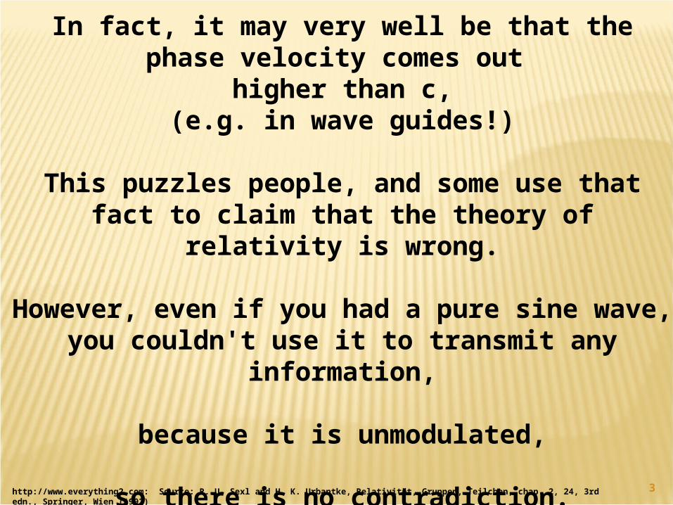
The change in the rate of phase change (fixed change in frequency) observed at

receiver, with respect to stationary transmitter, is proportional to velocity of

moving transmitter.

€

fr x , t( ) = f0 −

f0

cv

c is speed of waves in medium,

v is velocity of

transmitter

(this is classical, not relativistic)


20http://electron9.phys.utk.edu/phys135d/modules/m10/doppler.htm

If you knew the frequency transmitted by the moving transmitter.

You can use the

beat frequency

produced by combining the received signal with a receiver generated signal that is at

the transmitted frequency

to determine the speed.

21

But we can do more.

We can

count the (beat) cyclesor measure the (beat) phase

of the beat signal as a function of time.

This will give us the change in distance.(as will velocity times time)


22

So we can write

Beat phase ( t ) = change in distance to transmitter + constant

Beat phase ( at t = tfixed ) = distance to transmitter + constant

Note the arbitrary constant –can redo measurements from another

position(along trajectory of moving transmitter)

and get same result(initial phase measurement will be different,

but that will not change the frequency or distance estimation)


23www.ws.binghamton.edu/fowler/fowler personal page/ EE522_files/CRLB for Dopp_Loc Notes.pdf

http://www.cls.fr/html/argos/general/doppler_gps_en.html

Next – move the receiver off the path of the transmitter

(and can also let the transmitter path be arbitrary, now have to deal with vectors.)

€

fr x , t( ) = f0 −

f0

cr v t( ) •

r u t( )

24

Can solve this for

Location of stationary transmitter from a moving receiver (if you know x and v of

receiver – how SARSAT, ELT, EPIRB’s [Emergency Position Indicating Radio

Beacon ] work [or used to work – now also transmit location from GPS])

Location of moving transmitter(solve for x and v of transmitter)

from a stationary receiver(if you know x of receiver)

(Doppler shift, change in frequency, more useful for estimating velocity than position.

Integrate Doppler phase to get position.)

25http://www.npwrc.usgs.gov/perm/cranemov/location.htm


Apply this to GPS So far we have

Satellite carrier signalMixed with copy in receiver

After “low pass filter” – left with beat signal

Phase of beat signal equals reference phase minus received phase plus unknown integer

number full cycles

From here on we will follow convention and call

- Carrier beat phase --Carrier phase –

(remember it is NOT the phase of the incoming signal)


Consider the observation of satellite S

We can write the observed carrier (beat) phase as

€

ΦS T( ) = φ T( ) − φS T( ) − N S

Receiver replica of signal

Incoming signal received from satellite S

Receiver clock time


Now assume that the phase from the satellite received at time T is equal to what

it was when it was transmitted from the satellite

(we will eventually need to be able to model the travel time)

€

φS x,y,z,T( ) = φtransmitS x S , y S,zS ,T S

( )


€

ΦS T( ) = φ T( ) − φS T( ) − N S

Use from before for receiver time

€

T t( ) =φ t( ) − φ0( )

f0

€

φ T( ) = f0T + φ0

φtransmitS T S

( ) = f0TtransmitS + φ0

S

€

ΦS T( ) = f0T + φ0 − f0TtransmitS − φ0

S − N S

ΦS T( ) = f0 T − TtransmitS

( ) + φ0 − φ0S − N S

So the carrier phase observable becomes


€

ΦS T( ) = f0 T − TtransmitS

( ) + φ0 − φ0S − N S

Terms with S are for each satelliteAll other terms are equal for all observed

satellites

(receiver 0 should be same for all satellites– no interchannel bias, and

receiver should sample all satellites at same time – or interpolate measurements to same

time)

T S and N S will be different for each satelliteLast three terms cannot be separated (and will not be an integer) – call them “carrier

phase bias”


€

ΦAj TA( ) = f0 TA ,received − T j ,transmited

( ) + φ0A− φ0

j − NAj

Now we will convert carrier phase to range

(and let the superscript S-> satellite number, j,

to handle more than one satellite, and

add a subscript for multiple receivers, A,to handle more than one receiver.)


€

ΦAj TA( ) = f0 TA − T j

( ) + φ0A− φ0

j − NAj

We will also drop the “received” and “transmitted” reminders.

Times with superscripts will be for the transmission time by the satellite.

Times with subscripts will be for the reception time by the receiver.


If we are using multiple receivers, they should all sample at

exactly the same time(same value for receiver clock time).

Values of clock times of sample – epoch.

With multiple receivers the clocks are not perfectly synchronized, so the true

measurement times will vary slightly.

Also note – each receiver-satellite pair has its own carrier phase ambiguity.


carrier phase to rangeMultiply phase (in cycles, not radians) by

wavelength to get “distance”

€

LAj TA( ) = λ 0ΦA

j TA( )

LAj TA( ) = λ 0 f0 TA − T j

( ) + φ0A− φ0

j − NAj

( )

LAj Tk( ) = c TA − T j

( ) + λ 0 φ0A− φ0

j − NAj

( )

LAj TA( ) = c TA − T j

( ) + BAj

is in units of meters

is “carrier phase bias” (in meters)(is not an integer)€

LAj TA( )

€

BAj


This equation looks exactly like the equation for pseudo-range

€


( ) + BAj

That we saw before

€

PRS = ρ R

S tR , t S( ) + τ R −τ S

( ) c = ρ RS tR , t S( ) + cδ t

a distance


This equation also holds for both

L1 and L2

Clock biases same, but ambiguity different(different wavelengths)

€


( ) + BAj

pseudo-range constant


Added a few things related to propagation of waves

Delay in signal due to

Troposphere – Ionosphere –

(ionospheric term has “-” since phase velocity increases)

€


( ) + BAj

LAj TA( ) = ρ A

j tA , t j( ) + cτ A − cτ j + ZA

j − IAj + BA

j

Now that we have things expressed as “distance” (range)

Follow pseudo range development

€

ZAj

€

−IAj


Delay in signal due to

Troposphere +Ionosphere +

(ionospheric term now has “+” since group velocity to first order is same magnitude

but opposite sign as phase velocity)

€

PAj Tk( ) = c TA − T j

( )

PAj TA( ) = ρ A


j + IAj

Can include these effects in pseudo range development also

€

ZAj

€

−IAj


AAA Tt

Now we have to fix the time

So far our expression has receiver and satellite clock time

-Not true time

Remember that the true time is the clock time adjusted by the clock bias


AAA Tt

We know TA exactly

(it is the receiver clock time which is written into the observation file – called a “time

tag”)

But we don’t know A

(we need it to an accuracy of 1 sec)


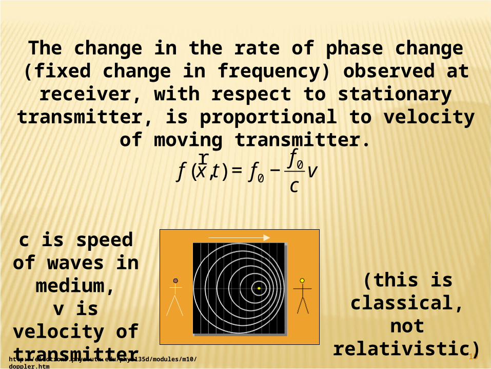
How to estimate A

- Use estimate of A from pseudo range point positioning

(if have receiver that uses the codes)

- LS iteration of code and phase data simultaneously

- If know satellite position and receiver location well enough (300 m for receiver – 1

sec of distance) can estimate it(this is how GPS is used for time transfer, once initialized can get time with only one

satellite visible [if don’t loose lock])

- Modeling shortcut – linearize (Taylor series)

42

Eliminating clock biases using differencing


€

LAj TA( ) = ρ A


j − IAj + BA

j

Return to our model for the phase observable

clock error - satellite

clock error - receiver

What do we get if we combine measurements made by two receivers

at the same epoch?


€

LAj TA( ) = ρ A


j − IAj + BA

j

LBj TB( ) = ρ B

j tB , t j( ) + cτ B − cτ j + ZB

j − IBj + BB

j

ΔLABj = LA

j TA( ) − LBj TB( )

Define the single difference

Use triangle to remember is difference between satellite (top)

and two receivers (bottom)


€

ΔLABj = LA

j TA( ) − LBj TB( )

ΔLABj = ρ A

j - ρ Bj + cτ A − cτ B − cτ j + cτ j

+ ZAj − ZB

j − IAj + IB

j + BAj − BB

j

ΔLABj = Δρ AB

j + Δcτ AB + ΔZABj − ΔIAB

j + ΔBABj

Satellite time errors cancel(assume transmission times are same –

probably not unless range to both receivers from satellite the same)

If the two receivers are close together the tropospheric and ionospheric terms also

(approximately) cancel.


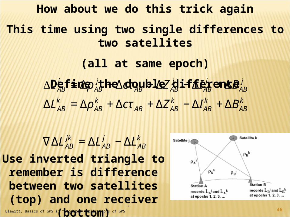
How about we do this trick again

This time using two single differences to two satellites

(all at same epoch)

Define the double difference

€

ΔLABj = Δρ AB

j + Δcτ AB + ΔZABj − ΔIAB

j + ΔBABj

ΔLABk = Δρ AB

k + Δcτ AB + ΔZABk − ΔIAB

k + ΔBABk

∇ΔLABjk = ΔLAB

j − ΔLABk

Use inverted triangle to remember is difference between two satellites (top) and one receiver

(bottom)


€

∇ΔLABjk = Δρ AB

j − Δρ ABk + Δcτ AB − Δcτ AB

+ ΔZABj − ΔZAB

k + ΔIABj − ΔIAB

k + ΔBABj − ΔBAB

k

∇ΔLABjk =∇Δρ AB

jk +∇ΔZABjk −∇ΔIAB

jk +∇ΔBABjk

Now we have gotten rid of the receiver clock bias terms

(again to first order – and results better for short baselines)

Double differencing- removes (large) clock bias errors

-approximately doubles (smaller) random errors due to atmosphere, ionosphere, etc.

(no free lunch)- have to be able to see satellite from both

receivers.


Next – what is the ambiguity term after double difference

(remembering definition of )

€

∇ΔBABjk = ΔBAB

j − ΔBABk

∇ΔBABjk = BA

j − BBj

( ) − BAk − BA

k( )

∇ΔBABjk = λ 0 φ0A

− φ0j − NA

j( ) − λ 0 φ0B

− φ0j − NB

j( ) +

- λ 0 φ0A− φ0

k − NAk

( ) + λ 0 φ0B− φ0

k − NBk

( )

∇ΔBABjk = −λ 0 NA

j − NBj − NA

k + NBk

( )

∇ΔBABjk = −λ 0NAB

jk

The ambiguity term reduces to an integer

€

BAj


€



jk − λ 0∇ΔNABjk

So our final

Double difference observation

is

One can do the differencing in either order

The sign on the ambiguity term is arbitrary


€

∇ΔLABjk i( ) =∇Δρ AB

jk i( ) +∇ΔZABjk i( ) −∇ΔIAB

jk i( ) −∇ΔNABjk i( )

∇ΔLABjk i +1( ) =∇Δρ AB

jk i +1( ) +∇ΔZABjk i +1( ) −

∇ΔIABjk i +1( ) −∇ΔNAB

jk i +1( )

δ i,i +1( )∇ΔLABjk =∇ΔLAB

jk i +1( ) −∇ΔLABjk i( )

We seem to be on a roll here, so let’s do it again.

This time(take the difference of double differences)

between two epochs

Equal if no loss of lock (no

cycle slip)

From E. Calais


€

δ i,i +1( )ΔLABjk =∇ΔLAB

jk i +1( ) −∇ΔLABjk i( )

δ i,i +1( )ΔLABjk = δ i,i +1( )∇ΔρAB

jk i( ) +

δ i,i +1( )∇ΔZABjk i( ) −δ i,i +1( )∇ΔIAB

jk i( )

So now we have gotten rid of the integer ambiguity

If no cycle slip – ambiguities removed.

If there is a cycle slip – get a spike in

the triple difference.

52From Ben Brooks

Raw Data from RINEX file: RANGEPlot of C1 (range in meters)

For all satellites for full day of data

53From Ben Brooks

Raw Data from RINEX file: RANGEPlot of P1 (range in meters)

For one satellite for full day of data

54From Ben Brooks

Raw Data from RINEX file: PHASE

55From Ben Brooks

Raw Data from RINEX file: RANGE DIFFERENCE

56From Ben Brooks

Raw Data from RINEX file: PHASE DIFFERENCE

57

-2000000

0

2000000

4000000

6000000

8000000

18.8 19.0 19.2 19.4 19.6 19.8

L1_phase L2_phase

Ph

ase

(cy

cle

s)

Hrs

Cycle slip at L2

http://www-gpsg.mit.edu/~tah/12.540/

Zoom in on phase observable

Without an (L1) and with an (L2) cycle slip

58http://www.gmat.unsw.edu.au/snap/gps/gps_survey/chap7/735.htm

Cycle slip shows up as spike in triple difference

(so can identify and fix)

Have to do this for “all” pairs of receiver-satellite pairs.

59

Effects of triple differences on estimation

Further increase in noise

Additional effect – introduces

correlation between observations in time

This effect substantial

So triple differences limited to identifying and fixing cycle slips.

60

Using double difference phase observations for relative positioning

First notice that if we make all double differences - even ignoring the obvious

duplications

€

∇ΔLABjk =∇ΔLAB

kj =∇ΔLBAkj =∇ΔLBA

jk

We get a lot more double differences than original data.

This can’t be (can’t create information).Blewitt, Basics of GPS in “Geodetic Applications of GPS”

61

€

LABjk = LA

j − LBj

( ) − LAk − LB

k( )

LABjl = LA

j − LBj

( ) − LAl − LB

l( )

LABlk = LA

l − LBl

( ) − LAk − LB

k( )

Consider the case of 3 satellites observed by 2 receivers.

€

LABjk = LAB

jl − LABlk

LABjl = LAB

jk − LABlk

LABlk = LAB

jk − LABjl

Form the (non trivial) double

differences

Note that we can form any one from a linear

combination of the other two

(linearly dependent)We need a linearly independent set for Least Squares.Blewitt, Basics of GPS in “Geodetic Applications of GPS”

62Blewitt, Basics of GPS in “Geodetic Applications of GPS”€

LABjk ,LAB

jl{ } = Λj = LABab a = j;b ≠ j{ }

LABkj ,LAB

kl{ } = Λk = LABab a = k;b ≠ k{ }

LABlj ,LAB

lk{ } = Λl = LABab a = l;b ≠ l{ }

€

LABjk ,LAB

jl ,LABlk{ }

From the linearly dependent set

We can form a number of linearly independent subsets

Which we can then use for our Least Squares estimation.


How to pick the basis?

All linearly independent sets are “equally” valid

and should produce identical solutions.

Pick l such that reference satellite l has data at every epoch

Better approach is to select the reference satellite epoch by epoch

(if you have 24 hour data file, cannot pick one satellite and use all day – no satellite is

visible all day)

64

For a single baseline (2 receivers) that observe s satellites,

the number of linearly independent double difference

observations is

s-1



Next suppose we have more than 2 receivers.

We have the same situation

-all the double differences are not linearly independent.

As we just did for multiple satellites, we can pick a

reference station

that is common to all the double differences.

66

For a network of r receivers,

the number of linearly independent double difference

observations is

r-1

So all together we have a total of

(s-1)(r-1)

Linearly independent double differencesBlewitt, Basics of GPS in “Geodetic Applications of GPS”


€

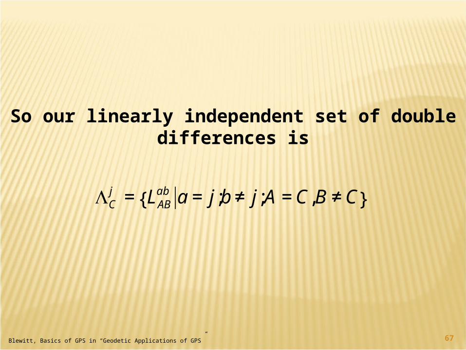
Cj = LAB

ab a = j;b ≠ j;A = C,B ≠ C{ }

So our linearly independent set of double differences is


Reference station method has problems when all receivers can’t see all satellites at

the same time.

Choose receiver close to center of network.


Even this might not work when the stations are very far apart.

For large networks may have to pick short baselines that connect the entire network.

Idea is to not have any closed polygons (which give multiple paths and therefore be

linearly dependent) in the network.

Can also pick reference station epoch per epoch.


If all the receivers see the same satellites at each epoch,

and data weighting is done properly,

then it does not matter which receiver and satellite we pick for the reference.


In practice, however,

the solution depends on our choices of reference receiver and satellite.

(although the solutions should be similar)

(could process all undifferenced phase observatons and estimate clocks at each epoch – ideally gives “better” estimates)


Double difference observation equations

€



jk −∇ΔNABjk

Start with

Simplify to

€

LABjk = ρ AB

jk − λ 0NABjk

€

∇ΔBy dropping the

And assuming are negligible

€

∇ΔZABjk &∇ΔIAB

jk


Processing double differences between two receivers results in a

Baseline solution

The estimated parameters include the vector between the two receivers (actually

antenna phase centers).

May also include estimates of parameters to model troposphere (statistical) and ionosphere (measured – dispersion).


Also have to estimate the

Integer Ambiguities

For each set of satellite-receiver double differences

75

We are faced with the same task we had before when we used

pseudo range

We have to

linearize

the problem in terms of the parameters we want to estimate


76http://dfs.iis.u-tokyo.ac.jp/~maoxc/its/gps1/node9.html

A significant difference between using thepseudo range,

which is a stand alone method, and using the

Phase,is that the phase is a differential method

(similar to VLBI).


So far we have cast the problem in terms of the distances to

the satellites,but we could recast it in terms of the

relative distancesbetween stations.


So now we will need multiple receivers.We will also have to use (at least one) as a

reference station.In addition to knowing where the satellites

are,We need to know the position of the

refrence station(s)to the same level of precision as we wish to estimate the position of the other stations.

79

fiducial positioning

Fiducial

Regarded or employed as a standard of reference, as in surveying.

http://dictionary.reference.com/search?q=fiducial

80http://dictionary.reference.com/search?q=fiducial

So now we have to assign the location of our fiducial station(s)

Can do this with

RINEX header position

VLBI position

Other GPS processing

etc.


So we have to

Write down the equations

Linearize

Solve

Earth Science Applications of Space Based Geodesy DES-7355 Tu-Th 9:40-11:05

Documents

Transcript of Earth Science Applications of Space Based Geodesy DES-7355 Tu-Th 9:40-11:05