Earth Maps

7/30/2019 Earth Maps

http://slidepdf.com/reader/full/earth-maps 1/11

R E F E R E E D P A P E R

Unfolding the Earth: Myriahedral Projections

Jarke J. van Wijk

Dept. of Mathematics and Computer Science, Technische Universiteit Eindhoven, Eindhoven, The Netherlands

Email: [email protected]

Myriahedral projections are a new class of methods for mapping the earth. The globe is projected on a myriahedron, a

polyhedron with a very large number of faces. Next, this polyhedron is cut open and unfolded. The resulting maps have a

large number of interrupts, but are (almost) conformal and conserve areas. A general approach is presented to decide

where to cut the globe, followed by three different types of solution. These follow from the use of meshes based on thestandard graticule, the use of recursively subdivided polyhedra and meshes derived from the geography of the earth. A

number of examples are presented, including maps for tutorial purposes, optimal foldouts of Platonic solids, and a map of

the coastline of the earth.

INTRODUCTION

Mapping the earth is an old and intensively studiedproblem. For about two thousand years, the challenge toshow the round earth on a flat surface has attracted many cartographers, mathematicians, and inventors, and hun-dreds of solutions have been developed. There are severalreasons for this high interest. First of all, the geography of the earth itself is interesting for all its inhabitants. Secondly,there are no perfect solutions possible such that the surfaceof the earth is depicted without distortion. Finally, factorssuch as the intended use of the map (e.g. navigation, visualisation, or presentation), the available technology (pen and ruler or computer), and the area or aspect to bedepicted lead to different requirements and hence todifferent optima.

A layman might wonder why map projection is a problemat all. A map of a small area, such as a district or city, is

almost free of distortion. So, to obtain a map of the earth without distortion one just has to stitch together a largenumber of such small maps. In this article we explore whathappens when this naive approach is pursued. We havecoined the term myriahedral for the resulting class of projections. A myriahedron is a polyhedron with a myriad of faces. The Latin word myriad is derived from the Greek word murioi , which means ten thousands or innumerable. We project the surface of the earth on such a myriahedron, we label its edges as folds or cuts, and fold it out to obtain aflat map.

In the next section, some basic notions on mapprojection are presented, and related work is shortly

described, followed by a section in which an overview of the approach employed here is given. Different solutions

are obtained by using different myriahedra and choices forthe edges to be cut, which are described in three separatesections. The use of graticule-based meshes, recursively subdivided polyhedra, and geographically aligned meshes

lead to different maps, each with their own strengths.Finally, the results are discussed.

BACKGROUND

The globe is a useful model for the surface of the earth.Locations on a globe (and the earth) are given by latitude wand longitude l. The position of a point p(w, l) on a globe with unit radius is (coslcosw, sinlcosw, sinw). Curves of constant w, such as the equator, are parallels; curves of constant l are meridians. A graticule is a set of parallels andmeridians at equal spacing in degrees.

Compared with a map, a globe has some disadvantages,

such as poor portability, and to obtain a more practicalsolution, the spherical globe has to be mapped to a flatsurface. This puzzle has intrigued many researchers for twothousand years. John P. Snyder has provided a fascinatingoverview of the history of map projection. In the following,references for map projections are only given if notdiscussed in his book (Snyder, 1993), to keep the numberof references within bounds. Introductions to map projection can be found in textbooks on cartography orgeographic visualisation (Robinson et al., 1995; Kraak andOrmeling, 2003; Slocum et al., 2003). Also on the webmuch information can be found, for instance in theextensive website developed by Furuti (2006).

The major problem of map projection is distortion.Consider a small circle on the globe. After projection on a

The Cartographic Journal Vol. 45 No. 1 pp. 32–42 February 2008 # The British Cartographic Society 2008

DOI: 10.1179/000870408X276594



map, this circle transforms into an ellipse, known as theTissot indicatrix, with semi-axes with lengths a and b . If a 5b for all locations, then angles between lines on the globeare maintained after projection: The projection is con-

formal . The classic example is the Mercator projection.Locally, conformality preserves shapes, but for larger areas

distortions occur. For example, in the Mercator projectionshapes near the poles are strongly distorted.

If ab 5 C for all locations on the map, then theprojection has the equal-area property: Areas are preservedafter projection. Examples are the sinusoidal, Lambert’scylindrical equal area and the Gall–Peters projection.

The problem is that for a double curved surface noprojection is possible that is both conformal and equal-area. Along a curve on the surface, such as the equator, bothconditions can be met; however, at increasing distance fromsuch a curve the distortion accumulates. Therefore,depending on the purpose of the map, one of theseproperties or a compromise between them has to be

chosen. Concerning distortion, uniform distances areanother aspect to be optimised. Unfortunately, no mapprojections are possible such that distances between any two positions are depicted on a similar scale, but one canaim at small variations overall or at proper depiction alongcertain lines.

Besides these constraints from differential geometry, mapprojection also has to cope with a topological issue. A sphere is a surface without a boundary, whereas a finite flatarea has to be bounded. Hence, a cartographer has todecide where to cut the globe and to which curve this cuthas to be mapped. Many choices are possible. One option,used for azimuthal projections, is to cut the surface of theglobe at a single point, and to project this to a circle,leading to very strong distortions at the boundary. Themost popular choice is to cut the globular surface along ameridian, and to project the two edges of this cut to anellipse, a flattened ellipse or a rectangle, where in the lasttwo cases the point-shaped poles are projected to curves.

The use of interrupts reduces distortion. For theproduction of globes, minimal distortion is vital forproduction purposes; hence gore maps are used, wherethe world is divided in for instance twelve gores. Goode’shomolosine projection (1923) is an equal-area projection,composed from twelve regions to form six interruptedlobes, with interrupts through the oceans. The projectionof the earth on unfolded polyhedra instead of rectangles or

ellipses is an old idea, going back to Da Vinci and Durer. Allregular polyhedra have been proposed as suitable candi-dates. Some examples are Cahill’s Butterfly Map (1909,octahedron) and the Dymaxion Map of Buckminster Fuller, who used a cuboctahedron (1946) and an icosahedron(1954). Steve Waterman has developed an appealingpolyhedral map, based on sphere packing.

Figure 1 visualises the trade-off to be made when dealing with distortion in map projection. An ideal projectionshould be equal-area, conformal, and have no interrupts;however, at most, two of these can be satisfied simulta-neously. Such projections are shown here at the corners of atriangle, whereas edges denote solutions where one of the

requirements is satisfied. Existing solutions can be posi-tioned in this solution space. Examples are given for some

cylindrical projections, with linear parallels and meridians.Most of the existing solutions, using no interrupts, arelocated at the bottom of the triangle. In this article, weexplore the top of the triangle, which is still terra incognita ,using geographic terminology. Or, in other words, wediscuss projections that are both (almost) equal area andconformal, but do have a very large number of interrupts.

Related issues have been studied intensively in the fieldsof computer graphics and geometric modelling, forapplications such as texture mapping, finite-element surface

meshing, and generation of clothing patterns. The problemof earth mapping is a particular case of the general surfaceparameterisation problem. A survey is given by Floater andHormann (2005). Finding strips on meshes has beenstudied in the context of mesh compression and meshrendering, for instance by Karni et al. (2002). Bounded-distortion flattening of curved surfaces via cuts was studiedby Sorkine et al. (2002). The work presented here has adifferent scope and ambition as this related work. Thegeometry to be handled is just a sphere. The aim is toobtain zero distortion, and we accept a large number of cuts. Finally, we aim at providing an integrated framework,offering fine control over the results, and explore the effectof different choices for the depiction of the surface of the

earth.

METHOD

We project the globe on a polyhedral mesh, label edges ascuts or folds, and unfold the mesh. We assume that thefaces of the mesh are small compared with the radius of theglobe, such that area and angular distortion are almostnegligible. We first discuss the labelling problem. A meshcan be considered as a (planar) graph G 5 (V , E ), consistingof a set of vertices V and undirected edges E that connect vertices. Consider the dual graph H 5 (V’ , E’ ), where each

vertex denotes a face of the mesh, and each edgecorresponds to an edge of the original graph, but now

Figure 1. Distortion in map projection

Unfolding the Earth: Myriahedral Projections 33



connecting two faces instead of two vertices (Figure 2). After labelling edges as folds and cuts, we obtain twosubgraphs H f and H c, where all edges of each subgraph arelabelled the same. The labelling of edges should be donesuch that

N the foldout is connected. In other words, in H f a pathshould exist from any node (face of the mesh) to any other node.

N the foldout can be flattened. Hence, in H f no cyclesshould occur, otherwise this condition cannot be met.

Taken together, these constraints imply that H f should be aspanning tree of H . Also, the subgraph G c of G with only

edges labelled as cuts should be a spanning tree of G . Thiscan be seen as follows. All vertices should have one or morecuts in the set of neighbouring edges (otherwise the foldoutcan not be flattened), and cycles in the cuts would lead to asplit of the foldout. The set of cuts unfolds to a singleboundary, with a length of twice the sum of lengths of thecuts.

There is a third constraint to be satisfied: The labellingshould be such that the foldout does not suffer from fold-overs. The folded out mesh should not only be planar, itshould also be single-valued. The use of an arbitrary spanning tree does lead to fold-overs in general. However, we found empirically that the schemes we use in the

following almost never lead to fold-overs, and we do notexplicitly test on this. The problem of fold-overs is complex,and we cannot give proofs on this. Nevertheless, it can beunderstood that fold-overs are rare by observing that thesphere is a very simple, uniform, convex surface; and also,the typical patterns that emerge are strips of triangles,connected to and radiating outward from a line or point, which strips rarely overlap.

The term spanning tree suggests a solution for labellingthe edges: Minimal spanning trees of graphs are a well-known concept in computer science. Assign a weight w (e i)to each of the edges e i, such that a high value indicates ahigh strength and that we prefer this edge to be a fold.

Next, calculate a maximal spanning tree H f (or a minimalspanning tree G c), i.e., a spanning tree such that the sum of

the weights its edges is maximal (or minimal). Thealgorithm to produce a myriahedral projection is now asfollows:

1. Generate a mesh;2. Assign weights to all edges;

3. Calculate a maximal spanning tree H f ;4. Unfold the mesh;5. Render the unfolded mesh.

In the following sections, we discuss various choices for thefirst two steps, here we describe the last three steps, whichare the same for all results shown.

For the calculation of the maximal spanning tree wefollowed the recommendations given by Moret andShapiro (1991). We use Prim’s algorithm (Prim, 1957) tofind a maximal spanning tree. Starting from a single vertex, iteratively, the neighbouring edge with thehighest weight and the corresponding vertex is added.This gives an optimal solution. The neighbouring edges

of the growing tree are stored in a priority queue, for which we use pairing heaps (Fredman, Sedgewick, Sleatorand Tarjan, 1986). The performance is O (|E | z |V | log|V |), where |E | and |V | denote the number of edges and vertices. In practice, optimal spanning trees are calculated within a second for graphs with ten thousands of edges and vertices.

Unfolding is straightforward. Assume that all faces of themesh are triangles. Faces with more edges can be handledby inserting interior edges with very high weights, such thatthese faces are never split up. Unfolding is done by firstpicking a central face, followed by recursive processing of adjacent faces. Consider two neighbouring triangles PQR

and RQS , and assume that the unfolded positions P 9

, Q 9

,and R 9 are known. Next, the angle a between RQS andthe plane of PQR is determined, and S 9 is calculated suchthat the new angle is a9, |QS | 5 |Q 9S 9| and |RS | 5 |R 9S 9|.The use of a9 5 0 gives a flat mesh, use of (for instance) a95 a(1 z cos(pt /T ))/2 gives a pleasant animation(examples are shown in http://www.win.tue.nl/, vanwijk/myriahedral).

The geography of the earth (or whatever image on aspherical surface has to be displayed) is mapped as a textureon the triangles. We use the maps of David Pape for this(Pape, 2001). When the triangles are large compared withthe radius of the globe, like in standard polyhedralprojections, the triangles have to be subdivided further to

control the projection in the interior. We use a simplegnomonic projection here.

Rendering maps for presentation purposes requiresproper anti-aliasing, because regular patterns and very thingaps have to be dealt with. For the images shown, 100-foldsupersampling per pixel with a jittered grid was used,followed by filtering with a Mitchell filter.

All images were produced with a custom developed,integrated tool to define meshes and weights, and tocalculate and render the results, running under MS Windows. Response times on standard PCs range frominstantaneous to a few seconds, which enables fastexploration of parameter spaces. Rendering of high

resolution, high quality maps can take somewhat longer,up to a few minutes.

Figure 2. (a) Mesh G ; (b) Dual mesh H ; (c) Cuts and folds; (d)Foldout

34 The Cartographic Journal



GRATICULES

The simplest way to define a mesh is to use the graticuleitself, and to cut along parallels or meridians. The resultscan be used as an introduction to map projection. A weightfor edges, using the value of w and l of the midpoint of anedge, can be defined as

w (w,l)~{(W wjw{w0jzW l mink

jl{l0z2pk j),

where W w and W l are overall scaling factors, and w0 and l0

denote where a maximal strength is desired. Different values for these lead to a number of familiar lookingprojections (Figure 3). The use of a high value for W wgives cuts along meridians. Dependent on the value of w0 a cylindrical projection (0u, equator), an azimuthalprojection (90u, North pole), or a conical projection(here 25u) is obtained when the meridian strips areunfolded. Use of a negative value for W w gives twohemispheres, each with an azimuthal projection. Themeridian at which to be centred can be controlled by usinga low value for W l and a suitable value for l0. The use of ahigh value for W l gives cuts along parallels. Unfolding these

parallels gives a result resembling the polyconic projectionof Hassler (1820).

The relation between a spatially varying weight w and thedecision where to cut and fold can be understood by considering Prim’s algorithm. Suppose, without loss of generality, that we start at a maximum of w and proceed toattach the edges with the highest weight. At some point,edges at the boundary will have approximately the same weight and, after a number of additions, a ring of faces isadded, with cuts in between neighbouring faces in this ring.Hence, edges aligned with contours of w typically turn intofolds, whereas edges aligned with gradients of w turn into

cuts.Each strip is almost free of angular or area distortion,

however, a large number of interrupts occur with varying widths. These gaps visualise, just like the Tissot indicatrix,the distortion that occurs when a non-interrupted map isused, and can be used to explain the basic problem of mapprojection. If we want to close these gaps, the strips mustbe broadened. However, to maintain an equal area, they have to be shortened, and to maintain the same aspect ratiothey have to be lengthened, which is not possiblesimultaneously. Also, it is clearly visible that mapping apoint (such as a pole) to a line leads to a strong distortion.

When the number of strips is increased, the gaps are less

visible, and the distortion is shown via the transparency of the map (Figure 4).

Figure 3. Graticular projections, derived from a 5u

graticule. 2592 polygons: a) cylindrical; b) conical; c) azimuthal; d) azimuthal, two hemi-spheres; e) polyconical




RECURSIVE SUBDIVISION

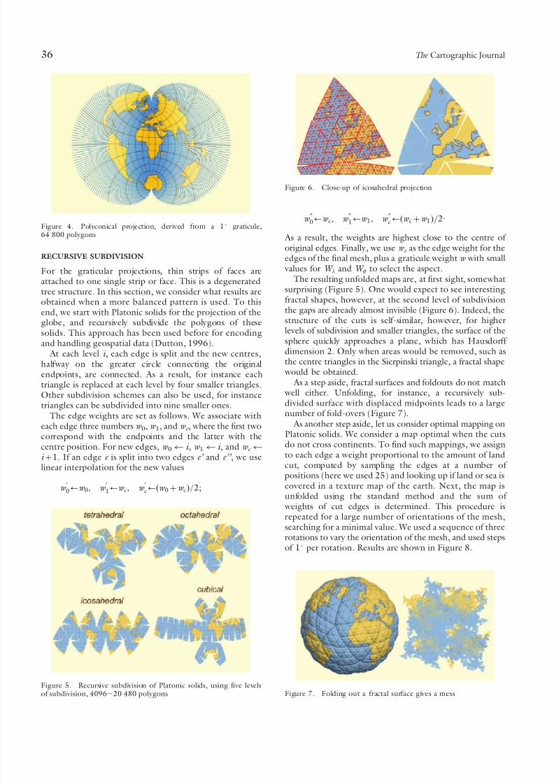
For the graticular projections, thin strips of faces areattached to one single strip or face. This is a degeneratedtree structure. In this section, we consider what results areobtained when a more balanced pattern is used. To thisend, we start with Platonic solids for the projection of theglobe, and recursively subdivide the polygons of thesesolids. This approach has been used before for encodingand handling geospatial data (Dutton, 1996).

At each level i , each edge is split and the new centres,halfway on the greater circle connecting the originalendpoints, are connected. As a result, for instance eachtriangle is replaced at each level by four smaller triangles.Other subdivision schemes can also be used, for instancetriangles can be subdivided into nine smaller ones.

The edge weights are set as follows. We associate witheach edge three numbers w 0, w 1, and w c , where the first twocorrespond with the endpoints and the latter with thecentre position. For new edges, w 0r i , w 1 r i , and w c ri z1. If an edge e is split into two edges e’ and e’’ , we uselinear interpolation for the new values

w 00/w 0, w

01/w c, w

0c/(w 0zw c)=2;

w 000/w c, w

001/w 1, w

00c/(w czw 1)=2:

As a result, the weights are highest close to the centre of original edges. Finally, we use w c as the edge weight for theedges of the final mesh, plus a graticule weight w with small values for W l and W w to select the aspect.

The resulting unfolded maps are, at first sight, somewhatsurprising (Figure 5). One would expect to see interestingfractal shapes, however, at the second level of subdivisionthe gaps are already almost invisible (Figure 6). Indeed, thestructure of the cuts is self-similar, however, for higherlevels of subdivision and smaller triangles, the surface of thesphere quickly approaches a plane, which has Hausdorff dimension 2. Only when areas would be removed, such asthe centre triangles in the Sierpinski triangle, a fractal shape would be obtained.

As a step aside, fractal surfaces and foldouts do not match well either. Unfolding, for instance, a recursively sub-divided surface with displaced midpoints leads to a large

number of fold-overs (Figure 7). As another step aside, let us consider optimal mapping on

Platonic solids. We consider a map optimal when the cutsdo not cross continents. To find such mappings, we assignto each edge a weight proportional to the amount of landcut, computed by sampling the edges at a number of positions (here we used 25) and looking up if land or sea iscovered in a texture map of the earth. Next, the map isunfolded using the standard method and the sum of weights of cut edges is determined. This procedure isrepeated for a large number of orientations of the mesh,searching for a minimal value. We used a sequence of threerotations to vary the orientation of the mesh, and used steps

of 1u

per rotation. Results are shown in Figure 8.

Figure 4. Polyconical projection, derived from a 1u graticule,64 800 polygons

Figure 5. Recursive subdivision of Platonic solids, using five levelsof subdivision, 4096220 480 polygons

Figure 6. Close-up of icosahedral projection

Figure 7. Folding out a fractal surface gives a mess




For the tetrahedron a perfect, and for the other platonic

solids an almost perfect, mapping is achieved. Except forthe tetrahedron, the resulting layout of the continents is thesame as the layout used by Fuller for his Dymaxion map. Heused a slightly modified icosahedron for his best-known version, but the version shown here reveals that hismodifications are not necessary per se.

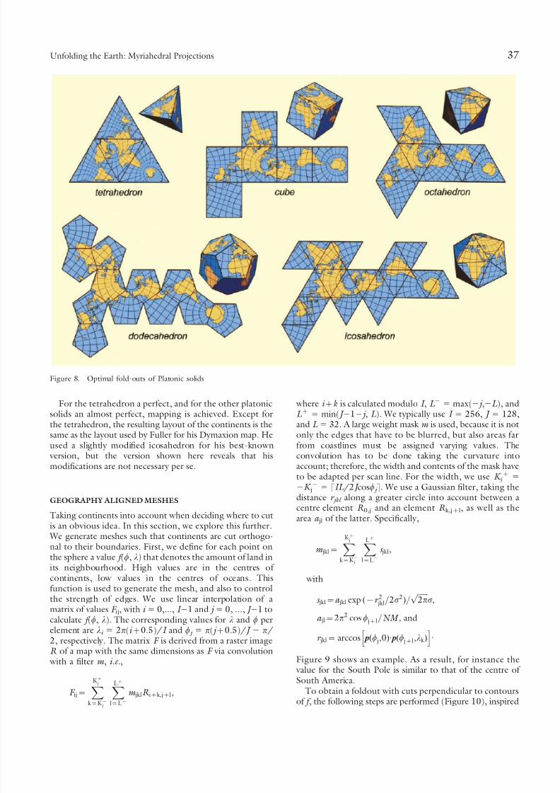
GEOGRAPHY ALIGNED MESHES

Taking continents into account when deciding where to cutis an obvious idea. In this section, we explore this further. We generate meshes such that continents are cut orthogo-nal to their boundaries. First, we define for each point on

the sphere a value f (w, l) that denotes the amount of land inits neighbourhood. High values are in the centres of continents, low values in the centres of oceans. Thisfunction is used to generate the mesh, and also to controlthe strength of edges. We use linear interpolation of amatrix of values F ij, with i 5 0,..., I 21 and j 5 0, ..., J 21 tocalculate f (w, l). The corresponding values for l and w perelement are li 5 2p(i z0.5)/I and w j 5 p( j z0.5)/ J 2 p/2, respectively. The matrix F is derived from a raster imageR of a map with the same dimensions as F via convolution with a filter m , i.e.,

F ij~XK z

j

k ~K { j

XL z

l~L {m jklR izk , jzl,

where i zk is calculated modulo I , L 2 5 max(2 j ,2L ), and

L z5

min( J 2

12

j , L ). We typically use I 5

256, J 5

128,and L 5 32. A large weight mask m is used, because it is notonly the edges that have to be blurred, but also areas farfrom coastlines must be assigned varying values. Theconvolution has to be done taking the curvature intoaccount; therefore, the width and contents of the mask haveto be adapted per scan line. For the width, we use K j

z5

2K j2

5 qIL /2 J cosw j r. We use a Gaussian filter, taking thedistance r jkl along a greater circle into account between acentre element R 0,j and an element R k,jzl, as well as thearea a jl of the latter. Specifically,

m jkl~ XK z

j

k ~K { jXL z

l~L {s jkl,

with

s jkl~a jkl exp ({r 2 jkl=2s2)= ffiffiffiffiffiffi 2p

p s,

a jl~2p2 cos w jzl=NM , and

r jkl~ arccos p(w j,0): p(w jzl,lk )h i

:

Figure 9 shows an example. As a result, for instance the value for the South Pole is similar to that of the centre of South America.

To obtain a foldout with cuts perpendicular to contoursof f , the following steps are performed (Figure 10), inspired

Figure 8. Optimal fold-outs of Platonic solids




by the anisotropic polygonal remeshing method of Alliezet al. (2003):

a. Generate mesh lines along and perpendicular tocontours of f with the algorithm of Jobard and Lefer(Jobard and Lefer, 1997);

b. Calculate intersections of these sets of lines, and derivepolygons;

c. Tesselate polygons with more than four edges; andfinally

d. Use the standard approach to decide on folds and cuts.

These steps are discussed in more detail.The algorithm of Jobard and Lefer (Jobard and Lefer,

1997) is an elegant and fast method to produce equally spaced streamlines for a given vector field. Starting from a

single streamline, new streamlines are repeatedly startedfrom seedpoints at a distance d from points of existingstreamlines, and traced in both directions. If such astreamline is too close to an existing streamline or when acycle is formed, the tracing is stopped. The time critical stepis to determine which points are close. The standardsolution is to use a rectangular grid for fast look-up. Herestreamlines are traced in (w, l) space, and the mapping tothe sphere has to be taken into account. We therefore usehorizontal strips of rectangles, where the number of rectangles per strip is proportional to cosw.

To obtain mesh lines along contours, the vector field

c (w,l)~

( f l,{

f w). ffiffiffiffiffiffiffiffiffiffiffiffiffiffiffiffiffiffiffiffiffiffiffiffiffiffiffi

cos2

w f 2

wz

f 2

lq

is traced; lines perpendicular to contours follow fromtracing the vector field

g (w,l)~( f w cos w, f l= cos w). ffiffiffiffiffiffiffiffiffiffiffiffiffiffiffiffiffiffiffiffiffiffiffiffiffiffiffi

cos2 w f 2wz f 2l

q , where

f l~L f (w,l)=Ll and f w~L f (w,l)=Lw:

The factors cosw in the definition of c and g follow from therequirements that we want these fields to have a unit

magnitude and to be orthogonal after projection on thesphere. Projection implies that components Dl of a vector(Dw, Dl) are scaled with a factor cosw, whereas the Dwcomponents keep their length. For the tracing, we use afourth order Runge–Kutta method with a fixed time step.

In the next step, crossings between these line sets arecalculated and the lines are cleaned up. Streamlines withoutcrossings are removed, neighbouring points of crossings areremoved from the streamlines, and heads and tails areremoved. Next, the resulting net is scanned and a set of

polygons, covering the sphere, is constructed. This gives aregular, rectangular mesh for a large part of the sphere, butalso and unfortunately, irregular polygons. This can beunderstood from the topology of vector fields, a well-known topic in the visualisation community (Helman andHesselink, 1991). Critical points are points where themagnitude of the vector field is zero. For the vector fieldsused here, these occur at maxima of f (centres of continents), minima of f (centres of oceans) and atsaddle-points of f (for instance between South Americaand Africa). The domain of a flow field can be tessellatedusing streamlines between these critical points, the so-calledseparatrices, which gives a topological decomposition of thedomain. For the vector fields used here, separatrices

typically run through valleys of f . When f is used to decide which edges to label as cuts, the surface breaks along those valleys, which in turn appear as overall boundaries.Downhill gradient lines of f , following g , bend into such valleys with a sharp turn or stop because a line at the otherside is too close, leading to irregular polygons.

We use a standard triangulation algorithm to tessellatepolygons with more than four edges. First, the polygon issplit into convex polygons, next, triangles are split off.Heuristics used are a preference for short inserted edges andavoidance of obtuse or very sharp angles. This is not perfect yet and leads to a somewhat fractured and irregularappearance of the map when unfolded. Improvement turns

out not to be simple. In an image like Figure 10(c) it is easy

Figure 9. From R to F via convolution with a Gaussian

Figure 10. Use of contours and gradients to derive a mesh: a) Jobard and Lefer algorithm; b) finding polygons; c) triangulation; d) decidingon cuts




to point at polygons where better choices could have beenmade, the hard part is to find methods that have no adverseeffect at other locations. For instance, introducing extrapoints and edges often leads to more irregularities, andtracing lines between critical points in advance gives wide

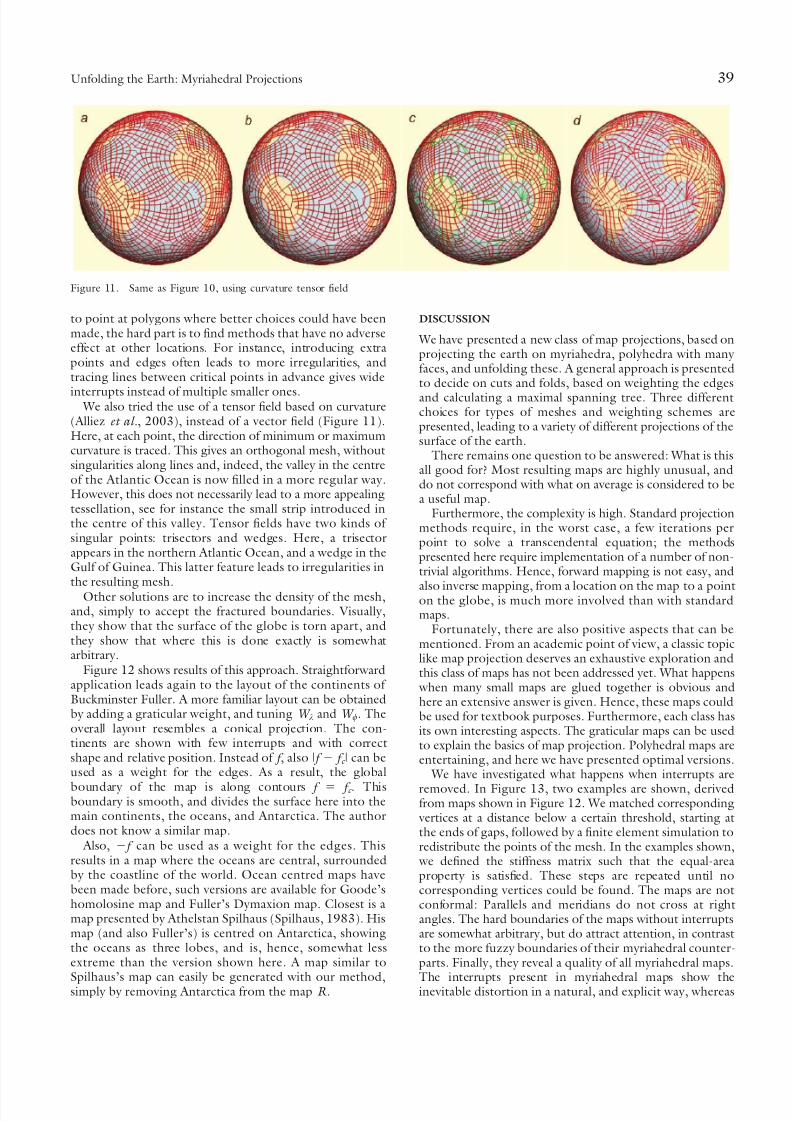
interrupts instead of multiple smaller ones. We also tried the use of a tensor field based on curvature

(Alliez et al., 2003), instead of a vector field (Figure 11).Here, at each point, the direction of minimum or maximumcurvature is traced. This gives an orthogonal mesh, withoutsingularities along lines and, indeed, the valley in the centreof the Atlantic Ocean is now filled in a more regular way.However, this does not necessarily lead to a more appealingtessellation, see for instance the small strip introduced inthe centre of this valley. Tensor fields have two kinds of singular points: trisectors and wedges. Here, a trisectorappears in the northern Atlantic Ocean, and a wedge in theGulf of Guinea. This latter feature leads to irregularities inthe resulting mesh.

Other solutions are to increase the density of the mesh,and, simply to accept the fractured boundaries. Visually,they show that the surface of the globe is torn apart, andthey show that where this is done exactly is somewhatarbitrary.

Figure 12 shows results of this approach. Straightforwardapplication leads again to the layout of the continents of Buckminster Fuller. A more familiar layout can be obtainedby adding a graticular weight, and tuning W l and W w. Theoverall layout resembles a conical projection. The con-tinents are shown with few interrupts and with correctshape and relative position. Instead of f , also | f 2 f c | can beused as a weight for the edges. As a result, the global

boundary of the map is along contours f 5 f c . Thisboundary is smooth, and divides the surface here into themain continents, the oceans, and Antarctica. The authordoes not know a similar map.

Also, 2 f can be used as a weight for the edges. Thisresults in a map where the oceans are central, surroundedby the coastline of the world. Ocean centred maps havebeen made before, such versions are available for Goode’shomolosine map and Fuller’s Dymaxion map. Closest is amap presented by Athelstan Spilhaus (Spilhaus, 1983). Hismap (and also Fuller’s) is centred on Antarctica, showingthe oceans as three lobes, and is, hence, somewhat lessextreme than the version shown here. A map similar to

Spilhaus’s map can easily be generated with our method,simply by removing Antarctica from the map R .

DISCUSSION

We have presented a new class of map projections, based onprojecting the earth on myriahedra, polyhedra with many faces, and unfolding these. A general approach is presentedto decide on cuts and folds, based on weighting the edgesand calculating a maximal spanning tree. Three differentchoices for types of meshes and weighting schemes arepresented, leading to a variety of different projections of thesurface of the earth.

There remains one question to be answered: What is thisall good for? Most resulting maps are highly unusual, anddo not correspond with what on average is considered to bea useful map.

Furthermore, the complexity is high. Standard projectionmethods require, in the worst case, a few iterations perpoint to solve a transcendental equation; the methodspresented here require implementation of a number of non-trivial algorithms. Hence, forward mapping is not easy, and

also inverse mapping, from a location on the map to a pointon the globe, is much more involved than with standardmaps.

Fortunately, there are also positive aspects that can bementioned. From an academic point of view, a classic topiclike map projection deserves an exhaustive exploration andthis class of maps has not been addressed yet. What happens when many small maps are glued together is obvious andhere an extensive answer is given. Hence, these maps couldbe used for textbook purposes. Furthermore, each class hasits own interesting aspects. The graticular maps can be usedto explain the basics of map projection. Polyhedral maps areentertaining, and here we have presented optimal versions.

We have investigated what happens when interrupts are

removed. In Figure 13, two examples are shown, derivedfrom maps shown in Figure 12. We matched corresponding vertices at a distance below a certain threshold, starting atthe ends of gaps, followed by a finite element simulation toredistribute the points of the mesh. In the examples shown, we defined the stiffness matrix such that the equal-areaproperty is satisfied. These steps are repeated until nocorresponding vertices could be found. The maps are notconformal: Parallels and meridians do not cross at rightangles. The hard boundaries of the maps without interruptsare somewhat arbitrary, but do attract attention, in contrastto the more fuzzy boundaries of their myriahedral counter-parts. Finally, they reveal a quality of all myriahedral maps.

The interrupts present in myriahedral maps show theinevitable distortion in a natural, and explicit way, whereas

Figure 11. Same as Figure 10, using curvature tensor field




in standard maps it is left to the viewer to guess where and which distortion occurs.

Methodologically interesting is that here a computerscience approach is used, whereas map projection istraditionally the domain of mathematicians, cartographers,and mathematical cartographers. Myriahedral projections

are generated using algorithms, partially originating fromflow visualisation, and not by formulas. Implementation is

not simple, but when the machinery is set up, a very large variety of maps can be generated just by changingparameters, such as W l, W w, F , f 0, s, and the size of thefaces used. This leaves much room for serendipity, andindeed, some of the maps shown here were discovered by accident.

Maps are not only used for navigation or visualisation,but also for decorative, illustrative and even rhetoric

Figure 12. Myriahedral projections with geography aligned meshes, 5500 polygons




(Proc. SDH7, Delft, Holland), 505–518, ed. by Kraak, M.-J. andMolenaar, M., Taylor & Francis, London.

Floater, M. S. and Hormann, K. (2005). ‘Surface parameterisation: atutorial and survey’, in Advances in multiresolution for geo-metric modelling , 157–186, ed. by Dodgson, N. A., Floater, M. S.and Sabin, M. A. (eds), Springer Verlag.

Fredman, M. L., Sedgewick, R., Sleator, D. D. and Tarjan, R. (1986).

‘The pairing heap: A new form of self-adjusting heap’, Algorithmica 1(1), 111–129.Furuti, C. A. (2006). ‘Map Projections’ http://www.progonos.com/

furuti/MapProj.Helman, J. L. and Hesselink, L. (1991). ‘Visualizing vector field

topology in fluid flows’, IEEE Computer Graphics and Applications 11(3), 36–46.

Iben, H. N. and O’Brien, J. F. (2006). ‘Generating surface crack patterns’, in Proceedings of the 2006 ACM SIGGRAPH/Eurographics Symposium on Computer Animation, SCA 2006, Vienna, Austria, 177–185, ed. by O’Sullivan, C. andPighin, F., Eurographics association, Aire-la-Ville, Switzerland.

Jobard, B. and Lefer, W. (1997). ‘Creating evenly-spaced stream-lines of arbitrary density’, in Visualization in Scientific Computing ’97, 43–56, ed. by Lefer, W. and Grave, M.,Springer Verlag.

Karni, Z., Bogomjakov, A. and Gotsman, C. (2002). ‘Efficient

compression and rendering of multi-resolution meshes’,Proceedings of IEEE Visualization 2002, 347–354, ed. by

Moorhead, R., Gross, M. and Joy, K.I., IEEE Computer Society Press.

Kraak, M.-J. and Ormeling, F. (2002). Cartography: Visualization of Geospatial Data (2nd edition), Prentice Hall, London.

Monmonier, M. (1991). How to Lie with Maps, University of Chicago Press, Chicago.

Moret, B. M. E. and Shapiro, H. D. (1991). ‘An empirical analysis of

algorithms for constructing a minimum spanning tree’, LectureNotes in Computer Science 555, 192–203, Springer Verlag.Pape, D. (2001). ‘Earth images’, www.evl.uic.edu/pape/data/Earth.Prim, R. (1957). ‘Shortest connection networks and some general-

isations’, Bell System Technical Journal 36, 1389–1401.Robinson, A. H., Morrison, J. L., Muehrcke, P. C. and Kimerling, A. J.

(1995). Elements of Cartography , Wiley.Slocum, T. A., McMaster, R. B., Kessler, F. C. and Howard, H. H.

(2003). Thematic Cartography and Geographic Visualization,Second Edition, Prentice Hall.

Snyder, J. P. (1993). Flattening the Earth: Two Thousand Years of Map Projections, University of Chicago Press.

Sorkine, O., Cohen-Or, D., Goldenthal, R. and Lischinski, D. (2002).‘Bounded-distortion piecewise mesh parameterisation’, Proceed-ings of IEEE Visualization 2002, 355–362, ed. by Moorhead,R., Gross, M. and Joy, K.I., IEEE Computer Society Press.

Spilhaus, A. (1983). ‘World ocean maps: The proper places to

interrupt’, Proceedings of the American Philosophical Society 127(1), 50–60.


Earth Maps

Documents

Transcript of Earth Maps