Earth and Planetary Science Letters 411 (2015) 27–36

Contents lists available at ScienceDirect

Earth and Planetary Science Letters

www.elsevier.com/locate/epsl

Rate of fluvial incision in the Central Alps constrained through joint

inversion of detrital 10Be and thermochronometric data

Matthew Fox a,b,∗, Kerry Leith c, Thomas Bodin a, Greg Balco b, David L. Shuster a,b

a Department of Earth and Planetary Science, University of California, Berkeley, CA, USAb Berkeley Geochronology Center, Berkeley, CA, USAc Chair of Landslide Research, Technische Universität München, Germany

a r t i c l e i n f o a b s t r a c t

Article history:Received 1 July 2014Received in revised form 22 November 2014Accepted 24 November 2014Available online xxxxEditor: T.M. Harrison

Keywords:detrital thermochronometryinner gorge formationlandscape evolutionfluvial erosion

We integrate constraints from published detrital thermochronometry and detrital 10Be concentrations in a single catchment to infer how erosion is shaping Alpine topography. We apply this analysis to the Codera watershed in the Bergell Intrusion, Central European Alps, where rivers have incised into a glacial valley. Because thermochronometric ages of bedrock samples increase with elevation, a distribution of detrital ages in river sediment provides a tracer for the source elevations of sediment within the catchment, while detrital 10Be concentrations provide constraints on rates of erosion. We find that modern erosion rates within the fluvial portion of the landscape are too low to permit the inferred ∼500 m of incision during the most recent interglacial. Based on the spatial pattern of modern erosion rates, we predict that if the incised fluvial valley was formed during interglacial periods only, it has formed over the last approximately 400,000 years.

© 2014 Elsevier B.V. All rights reserved.

1. Introduction

Measuring rates at which landscapes respond to changes in cli-mate and tectonics is essential to understand the processes and mechanisms facilitating erosion of the Earth’s surface. Quantifying erosion rates in mountain belts is, however, challenging as vari-ous approaches integrate erosion rate over different time intervals. These methods must therefore be supplemented by morphological observations describing the interaction of surface processes, and their temporal evolution within a landscape. In this study we ad-dress this issue with a method of determining spatial variations in modern erosion rate in a small catchment in the Swiss Alps using detrital thermochronometry and cosmogenic nuclide concen-trations.

An outstanding challenge in this area regards the determina-tion of the relative impact of principal erosional processes dur-ing glacial and interglacial cycles. Although these major climatic cycles provide a first-order control on surface processes, the rel-ative impact of associated processes on alpine morphology, and the distribution of present-day sediment production in formerly glaciated regions remains an open question. A promising avenue of research into this topic addresses the formation of deep bedrock

* Corresponding author.E-mail address: matthew.fox@berkeley.edu (M. Fox).

http://dx.doi.org/10.1016/j.epsl.2014.11.0380012-821X/© 2014 Elsevier B.V. All rights reserved.

gorges resulting from river incision into formerly glaciated Alpine topography during interglacial periods (Bonney, 1902; Korup and Schlunegger, 2007; Montgomery and Korup, 2011), or possibly re-sulting from subglacial meltwater (Dürst Stucki et al., 2012; Jansen et al., 2014). These inner gorges can be incised as much as 500 m below bedrock surfaces assumed to represent a former glacial valley floor, and if formed since the Last Glacial Maximum (LGM), would indicate rates of fluvial incision between 8.5 and 18 mm/yr, amongst the most rapid recorded on Earth (Montgomery and Ko-rup, 2011). Alternatively, assuming the most recent interglacial–glacial–interglacial transition (MIS 5–1) was typical of long-term (∼100 ka) Pleistocene climate cycles, the preservation of inter-glacial fluvial topography within valleys that have been through a full glacial cycle would indicate that long-term rates of flu-vial incision exceed those of glacial erosion in some portions of the landscape, where glaciation may locally protect the valley floor (Bonney, 1902; Garwood, 1910; McConnell, 1938; Lajeunesse, 2014; Tricart, 1960; De Graaff, 1996; Ostermann et al., 2006;Sanders et al., 2014).

The onset of fluvial incision into glacial landscapes within the Alps has been debated for over a century and difficulties in measuring incision rates have left this discussion unresolved. Arguments supporting post-Lateglacial (approximately 10–15 ka; Ivy-Ochs et al., 2008) onset for the incision of inner gorges were principally founded in the observation that they were located at

28 M. Fox et al. / Earth and Planetary Science Letters 411 (2015) 27–36

the base of glacial valleys (Penck, 1905). However, these arguments would not apply if the gorge morphology could be preserved through multiple glacial–interglacial cycles. Therefore, quantitativeestimates of erosion rate within fluvial gorges in the European Alps are required. By collecting cosmogenic nuclide exposure ages from bedrock at a range of elevations within a fluvial gorge, in the West-ern Alps, Valla et al. (2010) inferred Holocene incision rates by calculating the time between the exposure of rocks from different elevations. The calculated rates are greater than 10 mm/yr (Valla et al., 2010), suggesting the gorge was formed within the last 5–6 ka.

The hypothesis that significant bedrock gorges in the Alps can form by fluvial erosion during interglacial periods, however, is not consistent with long-term erosion rates inferred from regional thermochronometric data. Bedrock thermochronometry provides a key constraint on the total amount of erosion permitted over the last few millions of years, and by extension therefore also pro-vides an upper constraint on the total amount of fluvial erosion (Montgomery and Korup, 2011). If it is assumed that present-day inner gorges are the result of post-glacial fluvial incision, similar features should be expected to form during each interglacial. Fur-thermore, the amount of glacial erosion must have been sufficient to erase the inner gorge formed during each preceding interglacial. Predicted erosion based on present-day inner gorge depths would therefore exceed 10 km in the last 1 Myr, far in excess of the amount of exhumation constrained by thermochronometry in the Alps (Vernon et al., 2008).

Alternative lines of evidence may attest to the antiquity of Alpine inner gorges. Within several gorges across the Alps, de-posits older than the LGM are found, indicating that the gorges must be older than the LGM (Tricart, 1960; De Graaff, 1996;Ostermann et al., 2006; Sanders et al., 2014). Nested analyses of catchment-wide cosmic ray-produced nuclide concentrations have been conducted in the Entlebuch watershed (Central Swiss Alps). Data from these analyses support erosion rates as high as 3.5 mm/yr, and indicate that most recent erosion has been focused within the inner gorge (Berg et al., 2012). Although high for the Alps, these rates do not support the post-LGM inner gorge hypoth-esis unless erosion rates were much faster immediately following deglaciation.

In this paper, we investigate the potential for preservation of fluvial topography in the Codera watershed on the western side of the Bergell Intrusion (Central Swiss Alps) by combining exist-ing detrital thermochronometric data (Garver et al., 1999) with bedrock thermochronometric data (Wagner et al., 1977, 1979) to estimate the spatial distribution of erosion rates within the wa-tershed. We introduce a new method to simultaneously analyze these data with catchment-wide erosion rates derived from cosmic ray-produced 10Be concentration in detrital quartz (Norton et al., 2011). This allows us to explain the detrital age distribution and the cosmic ray-produced nuclide concentrations in terms of spatial variations in erosion rate. Our estimate of the spatial distribution of erosion rates, in turn, can be related to differential erosional processes across the fluvial and glacial portions of the landscape and thus used to evaluate hypotheses for the timescale over which these features formed.

2. Geological setting

2.1. The Bergell Intrusion

The Bergell Intrusion is delimited to the north–west and to the south by the Val Bregaglia and Valtellina, two large valleys that drain into Lake Como. Topographic relief is characteristically high, with the bottom of valleys at ∼300 m elevation and peaks ranging between 3000 and 4000 m elevation.

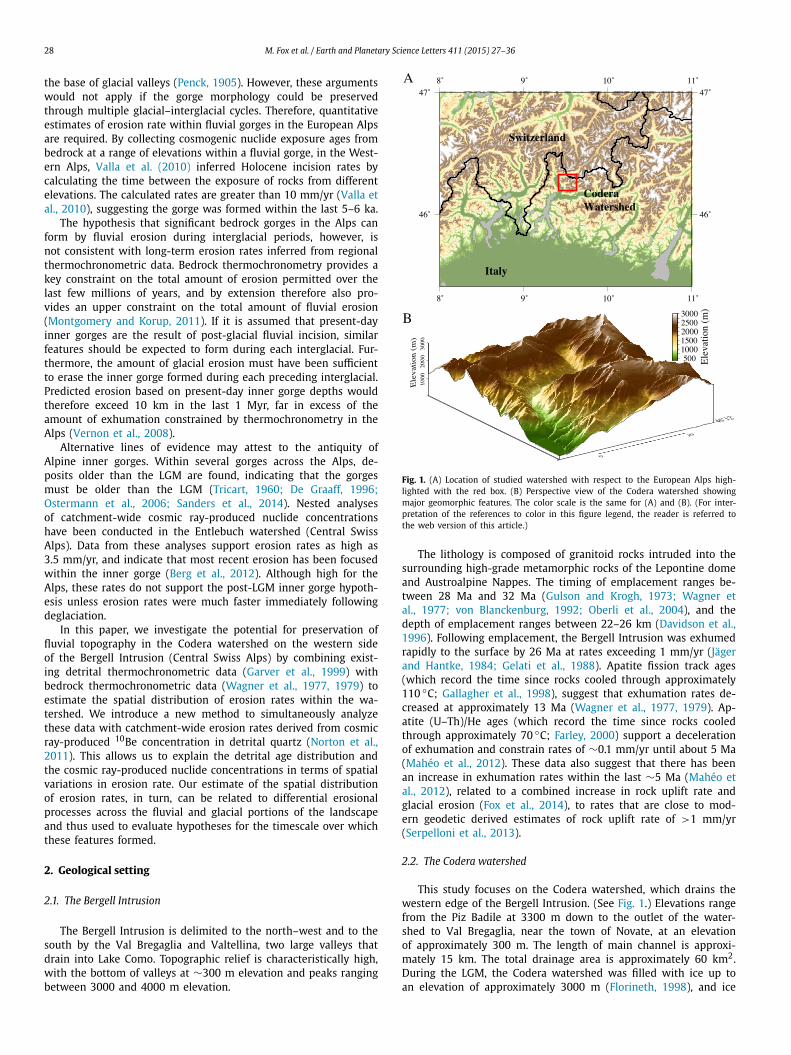
Fig. 1. (A) Location of studied watershed with respect to the European Alps high-lighted with the red box. (B) Perspective view of the Codera watershed showing major geomorphic features. The color scale is the same for (A) and (B). (For inter-pretation of the references to color in this figure legend, the reader is referred to the web version of this article.)

The lithology is composed of granitoid rocks intruded into the surrounding high-grade metamorphic rocks of the Lepontine dome and Austroalpine Nappes. The timing of emplacement ranges be-tween 28 Ma and 32 Ma (Gulson and Krogh, 1973; Wagner et al., 1977; von Blanckenburg, 1992; Oberli et al., 2004), and the depth of emplacement ranges between 22–26 km (Davidson et al., 1996). Following emplacement, the Bergell Intrusion was exhumed rapidly to the surface by 26 Ma at rates exceeding 1 mm/yr (Jäger and Hantke, 1984; Gelati et al., 1988). Apatite fission track ages (which record the time since rocks cooled through approximately 110 ◦C; Gallagher et al., 1998), suggest that exhumation rates de-creased at approximately 13 Ma (Wagner et al., 1977, 1979). Ap-atite (U–Th)/He ages (which record the time since rocks cooled through approximately 70 ◦C; Farley, 2000) support a deceleration of exhumation and constrain rates of ∼0.1 mm/yr until about 5 Ma (Mahéo et al., 2012). These data also suggest that there has been an increase in exhumation rates within the last ∼5 Ma (Mahéo et al., 2012), related to a combined increase in rock uplift rate and glacial erosion (Fox et al., 2014), to rates that are close to mod-ern geodetic derived estimates of rock uplift rate of >1 mm/yr (Serpelloni et al., 2013).

2.2. The Codera watershed

This study focuses on the Codera watershed, which drains the western edge of the Bergell Intrusion. (See Fig. 1.) Elevations range from the Piz Badile at 3300 m down to the outlet of the water-shed to Val Bregaglia, near the town of Novate, at an elevation of approximately 300 m. The length of main channel is approxi-mately 15 km. The total drainage area is approximately 60 km2. During the LGM, the Codera watershed was filled with ice up to an elevation of approximately 3000 m (Florineth, 1998), and ice

M. Fox et al. / Earth and Planetary Science Letters 411 (2015) 27–36 29

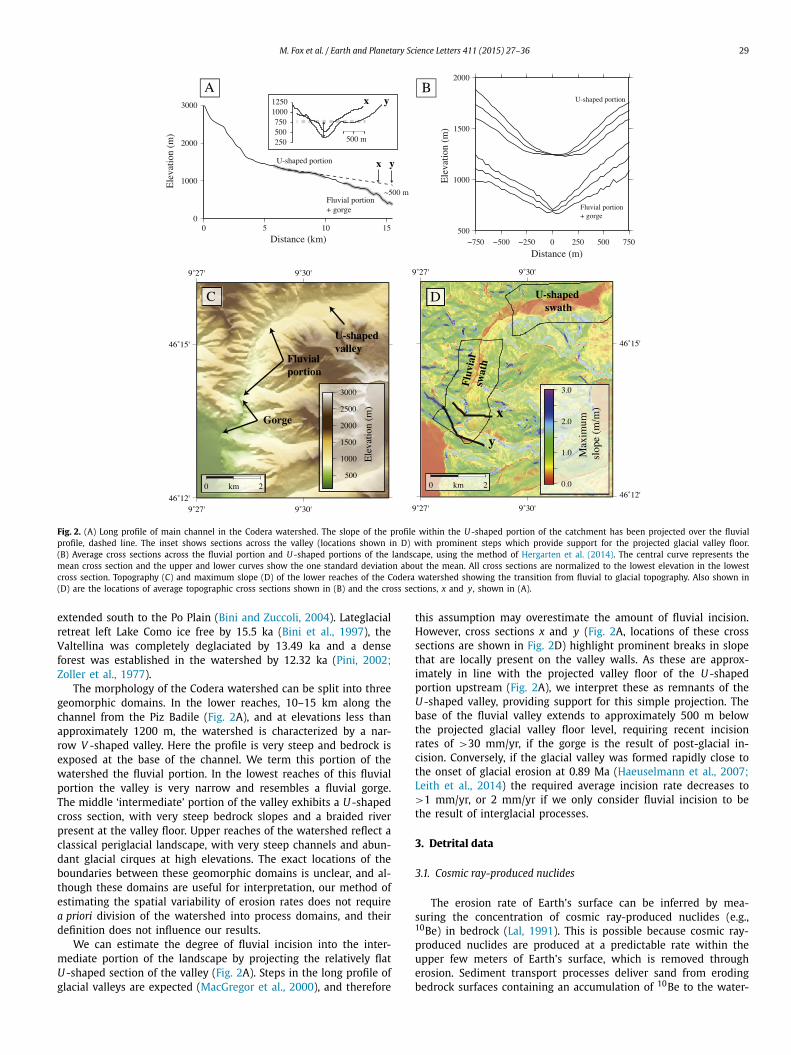
Fig. 2. (A) Long profile of main channel in the Codera watershed. The slope of the profile within the U -shaped portion of the catchment has been projected over the fluvial profile, dashed line. The inset shows sections across the valley (locations shown in D) with prominent steps which provide support for the projected glacial valley floor. (B) Average cross sections across the fluvial portion and U -shaped portions of the landscape, using the method of Hergarten et al. (2014). The central curve represents the mean cross section and the upper and lower curves show the one standard deviation about the mean. All cross sections are normalized to the lowest elevation in the lowest cross section. Topography (C) and maximum slope (D) of the lower reaches of the Codera watershed showing the transition from fluvial to glacial topography. Also shown in (D) are the locations of average topographic cross sections shown in (B) and the cross sections, x and y, shown in (A).

extended south to the Po Plain (Bini and Zuccoli, 2004). Lateglacial retreat left Lake Como ice free by 15.5 ka (Bini et al., 1997), the Valtellina was completely deglaciated by 13.49 ka and a dense forest was established in the watershed by 12.32 ka (Pini, 2002;Zoller et al., 1977).

The morphology of the Codera watershed can be split into three geomorphic domains. In the lower reaches, 10–15 km along the channel from the Piz Badile (Fig. 2A), and at elevations less than approximately 1200 m, the watershed is characterized by a nar-row V -shaped valley. Here the profile is very steep and bedrock is exposed at the base of the channel. We term this portion of the watershed the fluvial portion. In the lowest reaches of this fluvial portion the valley is very narrow and resembles a fluvial gorge. The middle ‘intermediate’ portion of the valley exhibits a U -shaped cross section, with very steep bedrock slopes and a braided river present at the valley floor. Upper reaches of the watershed reflect a classical periglacial landscape, with very steep channels and abun-dant glacial cirques at high elevations. The exact locations of the boundaries between these geomorphic domains is unclear, and al-though these domains are useful for interpretation, our method of estimating the spatial variability of erosion rates does not require a priori division of the watershed into process domains, and their definition does not influence our results.

We can estimate the degree of fluvial incision into the inter-mediate portion of the landscape by projecting the relatively flat U -shaped section of the valley (Fig. 2A). Steps in the long profile of glacial valleys are expected (MacGregor et al., 2000), and therefore

this assumption may overestimate the amount of fluvial incision. However, cross sections x and y (Fig. 2A, locations of these cross sections are shown in Fig. 2D) highlight prominent breaks in slope that are locally present on the valley walls. As these are approx-imately in line with the projected valley floor of the U -shaped portion upstream (Fig. 2A), we interpret these as remnants of theU -shaped valley, providing support for this simple projection. The base of the fluvial valley extends to approximately 500 m below the projected glacial valley floor level, requiring recent incision rates of >30 mm/yr, if the gorge is the result of post-glacial in-cision. Conversely, if the glacial valley was formed rapidly close to the onset of glacial erosion at 0.89 Ma (Haeuselmann et al., 2007;Leith et al., 2014) the required average incision rate decreases to >1 mm/yr, or 2 mm/yr if we only consider fluvial incision to be the result of interglacial processes.

3. Detrital data

3.1. Cosmic ray-produced nuclides

The erosion rate of Earth’s surface can be inferred by mea-suring the concentration of cosmic ray-produced nuclides (e.g., 10Be) in bedrock (Lal, 1991). This is possible because cosmic ray-produced nuclides are produced at a predictable rate within the upper few meters of Earth’s surface, which is removed through erosion. Sediment transport processes deliver sand from eroding bedrock surfaces containing an accumulation of 10Be to the water-

30 M. Fox et al. / Earth and Planetary Science Letters 411 (2015) 27–36

shed outlet. The concentration of 10Be in this sand therefore repre-sents an integrated signal of 10Be from across the entire watershed (Lal and Arnold, 1985; Brown et al., 1995; Granger et al., 1996;Bierman and Steig, 1996). Most studies employ a simplified rela-tionship between 10Be concentration in river sediments and basin-averaged erosion rate that reflects several assumptions: i) loss of 10Be from the basin by radioactive decay is negligible compared to loss by erosion; ii) all parts of the watershed contribute quartz to the sampled river sediment in proportion to their erosion rate; iii) the erosion rate is constant over the time during which the ob-served 10Be inventory accumulated; iv) the 10Be concentration has attained a steady state with respect to the erosion rate; and v) the amount of 10Be accumulated during sediment transport is negligi-ble.

10Be concentration in quartz has been measured from sand col-lected at the outlet of the Codera watershed and this concentration can be used to infer erosion rate integrated across the watershed (Norton et al., 2011). In the Codera watershed, the concentration of cosmic ray-produced 10Be has been interpreted in terms of an average erosion rate of 0.71 ± 0.13 mm/yr over the last ∼1 kyr (Norton et al., 2011).

3.2. Thermochronometric data

Detrital thermochronometric data have also been obtained from the Codera watershed (Garver et al., 1999). In the Bergell Intru-sion apatite fission track age increases with elevation (Wagner et al., 1977, 1979), and so different ages observed in the de-trital distribution can be related to specific elevations (Fig. 3A). As above, the processes of erosion and sediment transport de-liver sand from these specific elevations to the watershed outlet. Assuming the age–elevation relationship holds for the entire wa-tershed, the detrital distribution of apatite fission track ages re-flects the probability that sand is coming from a specific elevation within the watershed. This probability is a function of the areal extent of bedrock at this elevation and the spatial pattern of sur-face erosion rate (Brewer et al., 2006; Ruhl and Hodges, 2005;Stock et al., 2006; Vermeesch, 2007; McPhillips and Brandon, 2010;Avdeev et al., 2011; Tranel et al., 2011). As noted by Garver et al.(1999), the detrital age distribution (Fig. 3B) reflects ages from pre-dominantly low and high elevations. However, to date it has not been possible to determine whether this detrital age distribution is predominantly a function of the hypsometry of the watershed, variations in the slope of the age–elevation relationship, and/or spatial variations in erosion rate. We develop an approach to iden-tify spatial variations in erosion rate in the following section.

4. Methods

Detrital studies exploit the processes of erosion and sediment transport to obtain samples that are representative of the water-shed as a whole. The ability to relate sand-sized detritus obtained at the outlet to bedrock erosion is therefore a function of several factors: the spatial pattern of erosion rate across the watershed; the lithology across the watershed; the grain size produced as a function of erosion mechanisms across the watershed; and, due to the effects of comminution during sediment transport, the distance the sand has traveled since it was liberated from the bedrock.

The granitoid rocks of the Bergell Intrusion and metagranitic rocks from the surrounding Gruf Complex contain similar mineral assemblages, and we therefore assume lithological controls on the production of detrital material are minimal. In addition, the water-shed is small and steep, allowing us to assume there is little bias associated with grain size due to variations in sediment transport distance. Therefore, spatial variations in erosion rate due to differ-ences in geomorphic processes will be the main factor controlling

the delivery of sand from the bedrock to the outlet of the water-shed.

Given the above assumptions, the probability of observing a de-trital grain at the outlet with some characteristic representative of the bedrock is a function of the spatial pattern of erosion rate. As an example, the probability pd(τd) of observing a detrital age, τd , is the surface integral across the entire watershed, w , of the prob-ability of sand coming from a specific location ps(w) multiplied by the probability of observing τd given that location ps(τd|w) (where | means “given” within a Bayesian framework). Here we use pd to denote probability related to a detrital datum and pb to denote probability related to a bedrock datum. Formally, we can write,

pd(τd) =¨

w

pb(τd|w ′)ps

(w ′)dw ′, (1)

where, ps(w ′) is the erosion rate with respect to the erosion rate integrated across the watershed (i.e. ps(w) = e(w)/ w e(w ′)dw ′) as we can only constrain relative erosion rates.

4.1. Treatment of thermochronometric data

In order to estimate the likelihood of observing a specific detri-tal age, we need to estimate the likelihood of observing that age at every location in the catchment. As bedrock age increases with elevation, the likelihood of observing a given age of a crystal mea-sured in the detrital population at a bedrock location within the watershed, pb(τd|w), is a function of the elevation and expected spread of ages observed in single crystals taken from bedrock at that location. In other words, because of this expected spread, a specific crystal age observed in the detrital distribution is not di-agnostic of a specific elevation but rather a range of elevations. Previous approaches to parameterize pb(τd|w) have assumed a normal distribution for this spread (Duvall et al., 2012), however this does not capture the expected asymmetric spread of individ-ual crystals ages, which will ultimately make up the detrital age distribution (Brandon, 1996; Galbraith, 1990).

Vermeesch (2007) presented an approach to account for asym-metric spread in age due to the counting statistics of fission tracks in individual crystals. In this approach, the number of induced tracks measured in crystals from the detrital sample is mapped to an age distribution at a specific elevation through the following steps: 1) select a number of induced tracks (Ni ) at random from the measured detrital distribution; 2) rearrange the apatite fission track age equation (Hurford and Green, 1983) and calculate the number of spontaneous tracks for the specified bedrock age and Ni value; 3) sample a Poisson distribution for Ni and Ns; 4) use these replicates in the age equation to predict a single crystal age; 5) repeat steps 1–4 hundreds of times to produce a synthetic age distribution. Please see Vermeesch (2007), Glotzbach et al. (2013)for further details on this approach for inferring a detrital age distribution. For example, we calculated the expected individual apatite fission track crystal ages for a bedrock age of 15 Ma, using the distribution of induced tracks reported by Garver et al. (1999). A histogram of these ages shows that they range from 1 Ma to 55 Ma, and ages of approximately 15 Ma are calculated most fre-quently (Fig. 4). Ages produced with this approach can be used to calculate pb(τd|w), with the advantage that sample specific char-acteristics are accounted for. In order to improve computational efficiency, we note that the results of this approach can be approx-imated with a log–normal distribution with a mean of 15 Ma and variance (σ 2) of 20 Ma (Fig. 4). Therefore, we can write the proba-bility of observing a measured detrital age τd at a specific bedrock location, b(w) with known apatite fission track age is:

pb(τd|w) = 1∗ √ exp

(− (ln(τd) − b(w)∗)2

2(σ ∗)2

), (2)

σ τd 2π

M. Fox et al. / Earth and Planetary Science Letters 411 (2015) 27–36 31

Fig. 3. (A) Age elevation relationship for AFT data in the Bergell from Wagner et al. (1977, 1979). (B) Detrital AFT data from Garver et al. (1999) shown as a histogram and as the normalized cumulative density function (CDF) with individual ages plotted as black dots. The detrital dataset is composed of 114 ages.

Fig. 4. Expected crystal ages for a bedrock age of 15 Ma. The gray histogram shows the distribution of ages predicted using the method of Vermeesch (2007) using 1000 simulated ages. The black curve shows a log–normal probability density function with a mean age of 15 Ma and variance of 20 Ma2.

where b(w)∗ is the ‘location’ parameter and σ ∗ is the ‘scale’ pa-rameter defined as,

b(w)∗ = ln

(b(w)2√

σ 2 + b(w)2

), σ ∗ =

√ln

(1 + σ 2

b(w)2

). (3)

In turn, the likelihood of observing a set of nd (τ1, τ2, ... and τnd ) ages in a detrital sample, pd(D), is the product of the likeli-hood of observing each individual age:

pd(D) =nd∏

τd=1

pd(τd). (4)

The likelihood of observing an individual age pb(τb|w) is,

pb(τb|w) = 1

σ√

2πexp

(−1

2

(τb − b(w)

σb

)2), (5)

where σb is the uncertainty of the observed bedrock age. In turn, the likelihood of observing a set of (nb) bedrock ages pb(B) is then the product of the likelihood of observing each individual age,

pb(B) =nb∏

τb=1

pb(τb). (6)

By varying both ps(w) and b(w), we can maximize the prob-ability of predicting the observed bedrock ages and the detrital thermochronometric ages.

4.2. Treatment of cosmic ray-produced 10Be data

In general, erosion rate and 10Be production rate at a location within the watershed determines the 10Be concentration at that lo-cation. In turn ps(w) also determines the 10Be concentration in the detrital sample. Under the assumption of a spatially averaged ero-sion rate certain simplifications are justified. For example, the high inferred average erosion rate of 0.7 mm/yr (Norton et al., 2011), and associated young apparent exposure age of 1.03 ± 0.19 ka, imply that the bedrock 10Be concentration likely reached steady state approximately 1 kyr after deglaciation. However, here we al-low erosion rate to vary in space, thus parts of the watershed may erode at low rates such that non-steady state 10Be concentration after 10 ka is predicted. For this reason, we calculate 10Be concen-tration in space at each node of a 30 m DEM, C w (atoms g−1 yr−1), as a function of mass erosion rate, ε (kg m−2 yr−1), and exposure age, t (Myr):

C w = P (sp)w

λ + εwΛ(sp)

[1 − exp

(−

(λ + εw

Λ(sp)

)t

)]+ P (μ)w

λ + εwΛ(μ)

, (7)

where P (sp)w and P (μ)w are the production rate of 10Be due to spallation and muon reactions, respectively (atoms g−1 yr−1) cal-culated according to Stone (2000) and topographic shielding is calculated for each pixel in a 30 m DEM by assuming that the intensity of the cosmic ray flux is proportional to cos2.3(φ), where φ is the zenith angle (Gosse and Phillips, 2001). λ is the decay constant of 10Be (4.99 × 10−7 yr−1, after Chmeleff et al., 2010;Korschinek et al., 2010), εw is the sediment yield (g cm−2 yr−1) and εw = ρe(w) where ρ is density (2700 kg m−3) and e(w)

is the erosion rate (km/Myr), and Λ(sp) is the effective atten-uation length for spallogenic production of 10Be (1600 kg m−2). Λ(μ) is the effective attenuation length for muon production (15,000 kg m−2). The values for these parameters are taken from Balco et al. (2008).

The error introduced by not incorporating non-steady state ef-fects on 10Be concentration due to exposure of bedrock following deglaciation at 10 ka are shown in Fig. 5. Here, we predicted 10Be concentrations at a point in the watershed using Eq. (7) and calcu-lated the apparent erosion rate assuming that 10Be concentration is at a steady state with erosion rate. As expected, at low ero-sion rates the relative error is large because insufficient time has elapsed for steady-state to be reached. Therefore, the predicted erosion rate would be overestimated. However, at erosion rates greater than approximately 0.15 mm/yr steady state is reached rapidly and the effects of exposure following deglaciation at 10 ka are negligible.

The average 10Be concentration in the detrital sample, Cd , is equal to:

32 M. Fox et al. / Earth and Planetary Science Letters 411 (2015) 27–36

Fig. 5. The effects of incorporating deglaciation on catchment-wide erosion rate. Bedrock exposure occurred following Lateglacial deglaciation assumed to have oc-curred at 10 ka (Ivy-Ochs et al., 2008). For erosion rates less than 0.1 mm/yr, the error associated with assuming the 10Be is in steady state with the watershed wide erosion is reasonably large. This would lead to an underestimation of erosion rates if a steady state model was assumed.

Cd =¨

w

C w ps(

w ′)dw ′. (8)

In turn, the likelihood of observing the measured 10Be concentra-tion in the detrital sand, pd(Cd) is equal to

pd(Cd) = 1

σc√

2πexp

(−1

2

(Co − Cd

σc

)2), (9)

where Co is the observed 10Be concentration and σc is the mea-surement uncertainty. Therefore, by varying e(w), we can maxi-mize the probability of predicting the observed 10Be concentration.

4.3. The inverse problem

The inverse problem is to determine the spatial pattern of erosion rate e(w) and the bedrock age pattern b(w), that max-imize the likelihood of observing the detrital age distribution, the bedrock ages and the 10Be concentration (i.e. pd(D) ∗ pb(B) ∗pd(ND)).

We parameterize both e(w) and b(w) as a function of eleva-tion (Avdeev et al., 2011; Duvall et al., 2012). We use a series of nodes distributed in elevation to describe e(w) and erosion rate changes linearly between these nodes. For the lowest and highest nodes, erosion rate is held constant and extrapolated to the lowest (hmin) and highest (hmax) elevations within the watershed, respec-tively. Values describing the elevation and erosion rate positions of the nodes can be within the area defined by emin and emax for el-evations between hmin and hmax. For example, a pixel in the DEM at elevation hi that is located between the elevations of nodes at h1 and h2 will have an erosion rate of,

ei = e1 + hi

(e2 − e1

h2 − h1

). (10)

To describe b(w), we adopt an age elevation relationship (AER) based approach by inferring values not of τ and z, but instead, of τ and dτ/dz (Avdeev et al., 2011). Note, that we use z to de-scribe b(w) and h to describe e(w). Our approach ensures that age increases with elevation to be consistent with the observed pattern (Fig. 3). In this approach, the elevation of the lowest node is defined at an elevation lower than the outlet (here we used sea level). The “age” of this node is a free parameter. The age of the second node is also a free parameter and the elevation at this node is calculated based on the value of (dτ/dz)1. Therefore, a pixel in

the DEM at elevation hi that is located between elevations nodes at z1 and z2 will have a bedrock age, τi of,

τi = τ1 + (dτ/dz)1(hi − z1). (11)

Avdeev et al. (2011) presented a method to infer these func-tions based on a Bayesian probabilistic framework and this method forms the basis of our approach. Here we define two vectors to simplify the analysis: β is a vector containing model parame-ters that describe e(w) and b(w); A is a vector containing the observations (bedrock ages, detrital ages and detrital cosmic-ray produced nuclide concentration). In the Bayesian framework, the distributions of e(w) and b(w) that we wish to approximate are combined and termed the posterior probability distribution. The posterior probability distribution of the model parameters β given the dataset A is a product of the model likelihood function (which quantifies data fit) with the prior distribution of the model param-eters (which quantifies what is known about the parameters “pri-or” to the analysis): the posterior density is expressed as p(β|A); the likelihood function is p(A|β); and the prior probability is p(β). Therefore, p(β|A) is expressed as,

p(β|A) = Cp(A|β)p(β), (12)

where C is a constant that ensures that the posterior probability integrates to unity (Avdeev et al., 2011).

In reality, p(β|A) is multi-dimensional function that is challeng-ing to calculate analytically. Therefore, p(β|A) is instead approxi-mated numerically using a Markov Chain Monte Carlo algorithm to efficiently sample parameter space (Hastings, 1970). The MCMC algorithm is based on a random walk that samples the space of possible models (Hastings, 1970). At each step of the walk, a new value of a model parameter is proposed based on a perturbation from the current model. The value of the proposed parameter is drawn from a Gaussian distribution centered on the current model with a standard deviation defined by the user. The proposed model is accepted or rejected based on an acceptance criterion. This ac-ceptance criterion is the ratio of the probabilities of the current and proposed model, such that all models are accepted that reduce data misfit yet occasionally, models will be accepted that increase data misfit in proportion to the ratio of the likelihoods. The stan-dard deviation of the proposal distribution controls the rate at which the algorithm explores parameter space. Once a model is accepted, this model replaces the current model and a new model is once again generated as a perturbation of the current model. This process is typically repeated >10,000 times. Accepted models are asymptotically distributed according to the target distribution, and this ensemble is used to approximate the posterior probability density function.

4.4. Reversible jump Markov Chain Monte Carlo algorithm

Although Bayesian inference allows us to quantify the full state of knowledge we have about model parameters, the posterior dis-tribution still depends on choices made at the outset, such as the complexity of the model. Thus, the number of nodes describing e(w) and b(w) will control the complexity of e(w) and b(w) and, by extension, p(β|A). Therefore, we use a reversible jump Markov Chain Monte Carlo (rjMCMC) algorithm (Green, 1995) to calculate p(β|A), which also treats the numbers of nodes as free parame-ters. This approach is only described briefly here (see Gallagher et al., 2009, 2011; Sambridge et al., 2013, for reviews).

The rjMCMC algorithm is initialized with a series of random parameter values that describe e(w) and b(w). A new model is proposed based on a perturbation from the current model, and is accepted or rejected based on an acceptance criterion, as with

M. Fox et al. / Earth and Planetary Science Letters 411 (2015) 27–36 33

Fig. 6. Potential proposals to change erosion rate as a function of elevation. (A) Pro-posal 1: change elevation of a node. (B) Proposal 2: change erosion rate value of a node. (C) Proposal 3: Birth of a new node leading to increased the complexity. (D) Proposal 4: Death of a node leading to decreased complexity. Erosion rate at a specific elevation is linearly interpolated from the two bracketing elevations. How-ever, for elevations lower than the lowest node, or higher than the highest node, erosion rate is extrapolated to hmin or hmax, respectively.

the MCMC algorithm. There are eight distinct proposals that are possible: 1) the elevation of the node describing erosion rate can move (Move); 2) the erosion rate at a node can change (Change); 3) the number of nodes describing e(w) can be increased (Birth); and 4) the number of nodes describing e(w) can be decreased (Death); 5–8) the same proposals occur describing b(w) as out-lined in (1–4). Proposals (1–4) are highlighted in Fig. 6. The mag-nitude of the new values are drawn from Gaussian distributions centered on the current model with a specified standard deviation of θ1 through to θ8 for proposals (1) to (8).

Proposals are accepted based on the acceptance probability. For Move and Change proposals (i.e., (1), (2), (5) and (6)) the ac-ceptance probability is proportional to the likelihood ratio of the proposed to the current model. This ensures that proposals that improve data fit are always accepted and those which decrease it are accepted with probability equal to the ratios of the likelihoods. For Birth and Death proposals (i.e., (3), (4), (7), and (8)) the ac-ceptance criteria favor models that reduce data misfit yet penalize models that are overly complex.

The complex transdimensional posterior distribution is chal-lenging to appraise. To obtain an interpretable solution, we project the posterior distribution onto two different spaces, and simply consider two density plots of sampled e(w) and b(w). For e(w), this process requires that we discretize the parameter space de-scribing the probability p(e(w)|A), which is a 2-D area of size �e(w) �h into pixels and determine the frequency at which line segments describing e(w) intersect with each pixel. The resulting two dimensional histogram approximates the posterior probability of e(w). A similar distribution can be generated to approximate the posterior distribution of b(w).

5. Results

We ran the rjMCMC algorithm outlined above with the pa-rameters controlling the model perturbations tuned to provide ac-ceptance rates of 30–40%. We ran the chain for 500,000 models. The first 10,000 models form the ‘burn in’ phase, after which the Markov chain is thought to have converged. These first models are discarded from the posterior distribution.

Results are plotted as a function of elevation for both the elevation–erosion rate relationship and the age–elevation relation-ship (Fig. 7). In the mid- to upper-elevation ranges (1500–2700 m), erosion rates are low and well-resolved by the model. We also predict high rates within the fluvial portion of the landscape at elevations <1000 m (Fig. 7B), however these rates are not as well resolved. Differences in resolution, and therefore uncertainty, are expected due to the hypsometry of the watershed.

With the exception of a single age, the data comprising the AER are relatively well reproduced by the model (Fig. 7C). We predict that age increases slowly with elevation until about 12 Ma. Age then increases at approximately 0.4 km/Ma until 15 Ma and then the AER decreases again to approximately 0.05 km/Ma until 25 Ma. Additional numerical modeling would be required to interpret this AER in terms of an exhumation rate history. However, we note that the decrease in the slope of the AER suggests a decrease in long-term exhumation rate at approximately 12 Ma consistent with pre-vious interpretations of (U–Th)/He data from the Bergell (Mahéo et al., 2012; Fox et al., 2014). We also predict a 10Be concentra-tion at the outlet of the catchment of 15.1 ± 1.7(×104) atoms g−1

qtzwhich is in close agreement with the observed concentration of 16.9 ± 2.2(×104) atoms g−1

qtz (Norton et al., 2011).The average modern erosion rate within the fluvial section of

the landscape below approximately 1200 m is ∼1.8 mm/yr, calcu-lated as the weighted average of the posterior distribution. Erosion rate across the intermediate section is much lower at approxi-mately 0.6 mm/yr and this is in good agreement with the average watershed erosion rate constrained from the 10Be cosmic ray pro-duced nuclide concentration. Finally, we observe close agreement

Fig. 7. (A) Hypsometry of the Codera watershed. (B) Predicted modern erosion rate distribution as a function of elevation. (C) Predicted apatite fission track age elevation relationship. The colors relate to posterior probability and the black curves show the expected model, which is a weighted sum of the ensemble of models that make up the posterior distribution. (For interpretation of the references to color in this figure legend, the reader is referred to the web version of this article.)

34 M. Fox et al. / Earth and Planetary Science Letters 411 (2015) 27–36

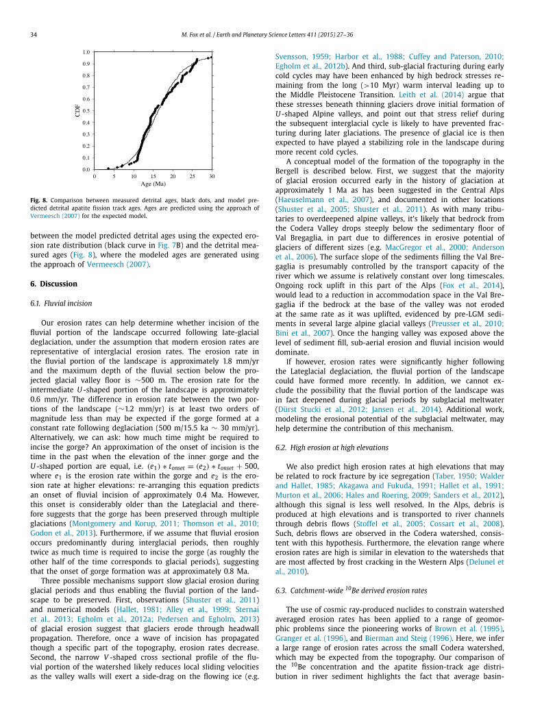
Fig. 8. Comparison between measured detrital ages, black dots, and model pre-dicted detrital apatite fission track ages. Ages are predicted using the approach of Vermeesch (2007) for the expected model.

between the model predicted detrital ages using the expected ero-sion rate distribution (black curve in Fig. 7B) and the detrital mea-sured ages (Fig. 8), where the modeled ages are generated using the approach of Vermeesch (2007).

6. Discussion

6.1. Fluvial incision

Our erosion rates can help determine whether incision of the fluvial portion of the landscape occurred following late-glacial deglaciation, under the assumption that modern erosion rates are representative of interglacial erosion rates. The erosion rate in the fluvial portion of the landscape is approximately 1.8 mm/yr and the maximum depth of the fluvial section below the pro-jected glacial valley floor is ∼500 m. The erosion rate for the intermediate U -shaped portion of the landscape is approximately 0.6 mm/yr. The difference in erosion rate between the two por-tions of the landscape (∼1.2 mm/yr) is at least two orders of magnitude less than may be expected if the gorge formed at a constant rate following deglaciation (500 m/15.5 ka ∼ 30 mm/yr). Alternatively, we can ask: how much time might be required to incise the gorge? An approximation of the onset of incision is the time in the past when the elevation of the inner gorge and the U -shaped portion are equal, i.e. (e1) ∗ tonset = (e2) ∗ tonset + 500, where e1 is the erosion rate within the gorge and e2 is the ero-sion rate at higher elevations: re-arranging this equation predicts an onset of fluvial incision of approximately 0.4 Ma. However, this onset is considerably older than the Lateglacial and there-fore suggests that the gorge has been preserved through multiple glaciations (Montgomery and Korup, 2011; Thomson et al., 2010;Godon et al., 2013). Furthermore, if we assume that fluvial erosion occurs predominantly during interglacial periods, then roughly twice as much time is required to incise the gorge (as roughly the other half of the time corresponds to glacial periods), suggesting that the onset of gorge formation was at approximately 0.8 Ma.

Three possible mechanisms support slow glacial erosion during glacial periods and thus enabling the fluvial portion of the land-scape to be preserved. First, observations (Shuster et al., 2011)and numerical models (Hallet, 1981; Alley et al., 1999; Sternai et al., 2013; Egholm et al., 2012a; Pedersen and Egholm, 2013)of glacial erosion suggest that glaciers erode through headwall propagation. Therefore, once a wave of incision has propagated though a specific part of the topography, erosion rates decrease. Second, the narrow V -shaped cross sectional profile of the flu-vial portion of the watershed likely reduces local sliding velocities as the valley walls will exert a side-drag on the flowing ice (e.g.

Svensson, 1959; Harbor et al., 1988; Cuffey and Paterson, 2010;Egholm et al., 2012b). And third, sub-glacial fracturing during early cold cycles may have been enhanced by high bedrock stresses re-maining from the long (>10 Myr) warm interval leading up to the Middle Pleistocene Transition. Leith et al. (2014) argue that these stresses beneath thinning glaciers drove initial formation of U -shaped Alpine valleys, and point out that stress relief during the subsequent interglacial cycle is likely to have prevented frac-turing during later glaciations. The presence of glacial ice is then expected to have played a stabilizing role in the landscape during more recent cold cycles.

A conceptual model of the formation of the topography in the Bergell is described below. First, we suggest that the majority of glacial erosion occurred early in the history of glaciation at approximately 1 Ma as has been suggested in the Central Alps (Haeuselmann et al., 2007), and documented in other locations (Shuster et al., 2005; Shuster et al., 2011). As with many tribu-taries to overdeepened alpine valleys, it’s likely that bedrock from the Codera Valley drops steeply below the sedimentary floor of Val Bregaglia, in part due to differences in erosive potential of glaciers of different sizes (e.g. MacGregor et al., 2000; Anderson et al., 2006). The surface slope of the sediments filling the Val Bre-gaglia is presumably controlled by the transport capacity of the river which we assume is relatively constant over long timescales. Ongoing rock uplift in this part of the Alps (Fox et al., 2014), would lead to a reduction in accommodation space in the Val Bre-gaglia if the bedrock at the base of the valley was not eroded at the same rate as it was uplifted, evidenced by pre-LGM sedi-ments in several large alpine glacial valleys (Preusser et al., 2010;Bini et al., 2007). Once the hanging valley was exposed above the level of sediment fill, sub-aerial erosion and fluvial incision would dominate.

If however, erosion rates were significantly higher following the Lateglacial deglaciation, the fluvial portion of the landscape could have formed more recently. In addition, we cannot ex-clude the possibility that the fluvial portion of the landscape was in fact deepened during glacial periods by subglacial meltwater (Dürst Stucki et al., 2012; Jansen et al., 2014). Additional work, modeling the erosional potential of the subglacial meltwater, may help determine the contribution of this mechanism.

6.2. High erosion at high elevations

We also predict high erosion rates at high elevations that may be related to rock fracture by ice segregation (Taber, 1950; Walder and Hallet, 1985; Akagawa and Fukuda, 1991; Hallet et al., 1991;Murton et al., 2006; Hales and Roering, 2009; Sanders et al., 2012), although this signal is less well resolved. In the Alps, debris is produced at high elevations and is transported to river channels through debris flows (Stoffel et al., 2005; Cossart et al., 2008). Such, debris flows are observed in the Codera watershed, consis-tent with this hypothesis. Furthermore, the elevation range where erosion rates are high is similar in elevation to the watersheds that are most affected by frost cracking in the Western Alps (Delunel et al., 2010).

6.3. Catchment-wide 10Be derived erosion rates

The use of cosmic ray-produced nuclides to constrain watershed averaged erosion rates has been applied to a range of geomor-phic problems since the pioneering works of Brown et al. (1995), Granger et al. (1996), and Bierman and Steig (1996). Here, we infer a large range of erosion rates across the small Codera watershed, which may be expected from the topography. Our comparison of the 10Be concentration and the apatite fission-track age distri-bution in river sediment highlights the fact that average basin-

M. Fox et al. / Earth and Planetary Science Letters 411 (2015) 27–36 35

scale erosion rates inferred from single measurements of sedi-mentary 10Be concentrations can obscure large intra-basin varia-tions in erosion rate (Brown et al., 1995; Bierman and Steig, 1996;Delunel et al., 2014).

7. Conclusions

We have developed a method to infer the spatial pattern of erosion rate using a joint analysis of bedrock and detrital ther-mochronometric ages and the detrital cosmic ray-produced nuclide concentration. Our approach is based on the work of Avdeev et al. (2011) however, here we have incorporated a reversible jump Markov chain Monte Carlo algorithm, enabling us to cast the in-verse problem in a fully non-linear probabilistic framework, and infer model complexity along with the spatial pattern of modern erosion rate and the thermochronometric age as a function of ele-vation.

If we assume that the modern erosion rate pattern is repre-sentative of interglacial periods, the spatial pattern of erosion rate allows us to estimate the onset of incision of the fluvial portion of the watershed. If we assume that we can project the modern ero-sion rate constrained for the fluvial portion of the landscape back through time, we predict that fluvial incision in the lower parts of the Codera watershed has been underway for approximately 0.4 Ma. However, the watershed has been glaciated for approxi-mately half of the last 1 Ma. Therefore, if we integrate the modern erosion rate at low elevations solely through interglacial periods, we would estimate the onset of fluvial incision to be ∼0.8 Ma.

Acknowledgements

We thank P. Vermeesch for stimulating discussions, and M. Trem-blay for comments on an early version of the manuscript. We also thank P. Valla and an anonymous reviewer for providing thorough and helpful reviews. This work has been supported by the Swiss National Science Foundation (P2EZP2_148793), the U.S. National Science Foundation grant EAR-1049988 (to D.L.S.) and the Ann and Gordon Getty Foundation. Figures were prepared using the Generic Mapping Tools (Wessel and Smith, 1998).

References

Akagawa, S., Fukuda, M., 1991. Frost heave mechanism in welded tuff. Permafr. Periglac. Process. 2 (4), 301–309.

Alley, R.B., Strasser, J.C., Lawson, D.E., Evenson, E.B., Larson, G.J., 1999. Glaciological and geological implications of basal-ice accretion in overdeepenings. In: Geolog-ical Society of America Special Papers, vol. 337, pp. 1–9.

Anderson, R.S., Molnar, P., Kessler, M.A., 2006. Features of glacial valley profiles sim-ply explained. J. Geophys. Res., Earth Surf. 111 (F1).

Avdeev, B., Niemi, N.A., Clark, M.K., 2011. Doing more with less: Bayesian estima-tion of erosion models with detrital thermochronometric data. Earth Planet. Sci. Lett. 305 (3), 385–395.

Balco, G., Stone, J.O., Lifton, N.A., Dunai, T.J., 2008. A complete and easily accessible means of calculating surface exposure ages or erosion rates from 10Be and 26Al measurements. Quat. Geochronol. 3 (3), 174–195.

Berg, F., Schlunegger, F., Akçar, N., Kubik, P., 2012. 10Be-derived assessment of accel-erated erosion in a glacially conditioned inner gorge, Entlebuch, Central Alps of Switzerland. Earth Surf. Process. Landf. 37 (11), 1176–1188.

Bierman, P., Steig, E.J., 1996. Estimating rates of denudation using cosmogenic iso-tope abundances in sediment. Earth Surf. Process. Landf. 21 (2), 125–139.

Bini, A., Zuccoli, L., 2004. Glacial history of the southern side of the central Alps, Italy. In: Quaternary Glaciations Extent and Chronology: Part I: Europe, vol. 2, p. 195.

Bini, A., Uggeri, A., Quinif, Y., 1997. Datazioni U/Th effettuate in Grotte delle Alpi (1986–1997): considerazioni sull’evoluzione del carsismo e del paleoclima. Geol. Insubrica 2 (1), 31–58.

Bini, A., Corbari, D., Falletti, P., Fassina, M., Perotti, C.R., Piccin, A., 2007. Morphology and geological setting of Iseo Lake (Lombardy) through multibeam bathymetry and high-resolution seismic profiles. Swiss J. Geosci. 100 (1), 23–40.

Bonney, T.G., 1902. Alpine valleys in relation to glaciers. Q. J. Geol. Soc. 58 (1–4), 690–702.

Brandon, M.T., 1996. Probability density plot for fission-track grain-age samples. Ra-diat. Meas. 26 (5), 663–676.

Brewer, I.D., Burbank, D.W., Hodges, K.V., 2006. Downstream development of a de-trital cooling-age signal: insights from 40Ar/39Ar muscovite thermochronology in the Nepalese Himalaya. In: Geological Society of America Special Papers, vol. 398, pp. 321–338.

Brown, E.T., Stallard, R.F., Larsen, M.C., Raisbeck, G.M., Yiou, F., 1995. Denudation rates determined from the accumulation of in situ-produced 10Be in the Luquillo experimental forest, Puerto Rico. Earth Planet. Sci. Lett. 129 (1), 193–202.

Chmeleff, J., von Blanckenburg, F., Kossert, K., Jakob, D., 2010. Determination of the 10Be half-life by multicollector ICP-MS and liquid scintillation counting. Nucl. Instrum. Methods Phys. Res., Sect. B, Beam Interact. Mater. Atoms 268 (2), 192–199.

Cossart, E., Braucher, R., Fort, M., Bourlès, D., Carcaillet, J., 2008. Slope instability in relation to glacial debuttressing in alpine areas (Upper Durance catchment, southeastern France): evidence from field data and 10Be cosmic ray exposure ages. Geomorphology 95 (1), 3–26.

Cuffey, K.M., Paterson, W.S.B., 2010. The Physics of Glaciers. Academic Press.Davidson, C., Rosenberg, C., Schmid, S.M., 1996. Synmagmatic folding of the base of

the Bergell pluton, Central Alps. Tectonophysics 265, 213–238.De Graaff, L., 1996. The fluvial factor in the evolution of alpine valleys and of ice-

marginal topography in Vorarlberg (W-Austria) during the Upper Pleistocene and Holocene. Z. Geomorphol., Suppl.bd 104, 129–159.

Delunel, R., Van Der Beek, P.A., Carcaillet, J., Bourlès, D.L., Valla, P.G., 2010. Frost-cracking control on catchment denudation rates: insights from in situ produced 10Be concentrations in stream sediments (Ecrins-Pelvoux massif, French West-ern Alps). Earth Planet. Sci. Lett. 293 (1–2), 72–83.

Delunel, R., Beek, P.A., Bourlès, D.L., Carcaillet, J., Schlunegger, F., 2014. Transient sediment supply in a high-altitude Alpine environment evidenced through a 10Be budget of the Etages catchment (French Western Alps). Earth Surf. Pro-cess. Landf. 39 (7), 890–899.

Dürst Stucki, M., Schlunegger, F., Christener, F., Otto, J.-C., Götz, J., 2012. Deepening of inner gorges through subglacial meltwater—an example from the UNESCO Entlebuch area, Switzerland. Geomorphology 139, 506–517.

Duvall, A.R., Clark, M.K., Avdeev, B., Farley, K.A., Chen, Z., 2012. Widespread late Cenozoic increase in erosion rates across the interior of eastern Tibet con-strained by detrital low-temperature thermochronometry. Tectonics 31 (3).

Egholm, D., Pedersen, V.K., Knudsen, M.F., Larsen, N.K., 2012a. Coupling the flow of ice, water, and sediment in a glacial landscape evolution model. Geomorphol-ogy 141, 47–66.

Egholm, D., Pedersen, V.K., Knudsen, M.F., Larsen, N.K., 2012b. On the importance of higher order ice dynamics for glacial landscape evolution. Geomorphology 141, 67–80.

Farley, K.A., 2000. Helium diffusion from apatite: general behavior as illustrated by Durango fluorapatite. J. Geophys. Res. 105 (B2), 2903–2914.

Florineth, D., 1998. Surface geometry of the Last Glacial Maximum (LGM) in the southeastern Swiss Alps (Graubünden) and its paleoclimatological significance. Eiszeitalt. Ggw. 48, 23–37.

Fox, M., Reverman, R., Herman, F., Fellin, M.G., Sternai, P., Willett, S.D., 2014. Rock uplift and erosion rate history of the Bergell Intrusion from the inversion of low temperature thermochronometric data. Geochem. Geophys. Geosyst. 15 (4), 1235–1257.

Galbraith, R., 1990. The radial plot: graphical assessment of spread in ages. Int. J. Radiat. Appl. Instrum., Part D Nucl. Tracks Radiat. Meas. 17 (3), 207–214.

Gallagher, K., Brown, R., Johnson, C., 1998. Fission track analysis and its applications to geological problems. Annu. Rev. Earth Planet. Sci. 26 (1), 519–572.

Gallagher, K., Charvin, K., Nielsen, S., Sambridge, M., Stephenson, J., 2009. Markov chain Monte Carlo (MCMC) sampling methods to determine optimal mod-els, model resolution and model choice for Earth Science problems. Mar. Pet. Geol. 26 (4), 525–535.

Gallagher, K., Bodin, T., Sambridge, M., Weiss, D., Kylander, M., Large, D., 2011. In-ference of abrupt changes in noisy geochemical records using transdimensional changepoint models. Earth Planet. Sci. Lett. 311 (1), 182–194.

Garver, J.I., Brandon, M.T., Roden-Tice, M., Kamp, P.J.J., 1999. Exhumation history of orogenic highlands determined by detrital fission-track thermochronology. Geol. Soc. (Lond.) Spec. Publ. 154 (1), 283–304.

Garwood, E., 1910. Features of alpine scenery due to glacial protection. Geogr. J. 36 (3), 310–336.

Gelati, R., Napolitano, A., Valdisturlo, A., 1988. La “Gonfolite Lombarda”: strati-grafia e significato nell’evoluzione del margine sudalpino. Riv. Ital. Paleontol. Stratigr. 94, 285–332.

Glotzbach, C., Beek, P., Carcaillet, J., Delunel, R., 2013. Deciphering the driving forces of erosion rates on millennial to million-year timescales in glacially impacted landscapes: an example from the Western Alps. J. Geophys. Res., Earth Surf. 118 (3), 1491–1515.

Godon, C., Mugnier, J., Fallourd, R., Paquette, J., Pohl, A., Buoncristiani, J., 2013. The Bossons glacier protects Europe’s summit from erosion. Earth Planet. Sci. Lett. 375, 135–147.

Gosse, J.C., Phillips, F.M., 2001. Terrestrial in situ cosmogenic nuclides: theory and application. Quat. Sci. Rev. 20 (14), 1475–1560.

36 M. Fox et al. / Earth and Planetary Science Letters 411 (2015) 27–36

Granger, D.E., Kirchner, J.W., Finkel, R., 1996. Spatially averaged long-term erosion rates measured from in situ-produced cosmogenic nuclides in alluvial sediment. J. Geol., 249–257.

Green, P.J., 1995. Reversible jump Markov chain Monte Carlo computation and Bayesian model determination. Biometrika 82 (4), 711–732.

Gulson, B.L., Krogh, T.E., 1973. Old lead components in the young Bergell Massif, south–east Swiss Alps. Computer 40, 239–252.

Haeuselmann, P., Granger, D.E., Jeannin, P.Y., Lauritzen, S.E., 2007. Abrupt glacial val-ley incision at 0.8 Ma dated from cave deposits in Switzerland. Geology 35 (2), 143–147.

Hales, T.C., Roering, J.J., 2009. A frost “buzzsaw” mechanism for erosion of the east-ern Southern Alps, New Zealand. Geomorphology 107, 241–253.

Hallet, B., 1981. Glacial abrasion and sliding: their dependence on the debris con-centration in basal ice. Ann. Glaciol. 2 (1), 23–28.

Hallet, B., Walder, J., Stubbs, C., 1991. Weathering by segregation ice growth in mi-crocracks at sustained subzero temperatures: verification from an experimental study using acoustic emissions. Permafr. Periglac. Process. 2 (4), 283–300.

Harbor, J.M., Hallet, B., Raymond, C.F., 1988. A numerical model of landform devel-opment by glacial erosion. Nature 333, 347–349.

Hastings, W.K., 1970. Monte Carlo sampling methods using Markov chains and their applications. Biometrika 57 (1), 97–109.

Hergarten, S., Robl, J., Stüwe, K., 2014. Extracting topographic swath profiles across curved geomorphic features. Earth Surf. Dyn. 2 (1), 97–104.

Hurford, A.J., Green, P.F., 1983. The zeta age calibration of fission-track dating. Chem. Geol. 41, 285–317.

Ivy-Ochs, S., Kerschner, H., Reuther, A., Preusser, F., Heine, K., Maisch, M., Kubik, P.W., Schlüchter, C., 2008. Chronology of the last glacial cycle in the European Alps. J. Quat. Sci. 23 (6–7), 559–573.

Jäger, E., Hantke, R., 1984. Evidenzen für die Vergletscherung eines alpinen Bergeller Hochgebirges an der Grenze Oligozän/Miozän. Int. J. Earth Sci. 73 (2), 567–575.

Jansen, J., Codilean, A., Stroeven, A., Fabel, D., Hättestrand, C., Kleman, J., Harbor, J., Heyman, J., Kubik, P., Xu, S., 2014. Inner gorges cut by subglacial meltwater during Fennoscandian ice sheet decay. Nat. Commun. 5.

Korschinek, G., Bergmaier, A., Faestermann, T., Gerstmann, U., Knie, K., Rugel, G., Wallner, A., Dillmann, I., Dollinger, G., Von Gostomski, C.L., et al., 2010. A new value for the half-life of 10Be by Heavy-Ion Elastic Recoil Detection and liquid scintillation counting. Nucl. Instrum. Methods Phys. Res., Sect. B, Beam Interact. Mater. Atoms 268 (2), 187–191.

Korup, O., Schlunegger, F., 2007. Bedrock landsliding, river incision, and transience of geomorphic hillslope-channel coupling: evidence from inner gorges in the Swiss Alps. J. Geophys. Res. 112 (F3), F03027.

Lajeunesse, P., 2014. Buried preglacial fluvial gorges and valleys preserved through Quaternary glaciations beneath the eastern Laurentide Ice Sheet. Geol. Soc. Am. Bull. 126 (3–4), 447–458.

Lal, D., 1991. Cosmic ray labeling of erosion surfaces: in situ nuclide production rates and erosion models. Earth Planet. Sci. Lett. 104 (2), 424–439.

Lal, D., Arnold, J., 1985. Tracing quartz through the environment. Proc. Indian Acad. Sci., Earth Planet. Sci. 94 (1), 1–5.

Leith, K., Moore, J.R., Amann, F., Loew, S., 2014. Subglacial extensional fracture de-velopment and implications for Alpine Valley evolution. J. Geophys. Res., Earth Surf. 119 (1), 62–81.

MacGregor, K.R., Anderson, R., Anderson, S., Waddington, E., 2000. Numerical simulations of glacial-valley longitudinal profile evolution. Geology 28 (11), 1031–1034.

Mahéo, G., Gautheron, C., Leloup, P., Fox, M., Tassant-Got, L., Douville, E., 2012. Neo-gene exhumation history of the Bergell massif (southeast Central Alps). Terra Nova 25 (2), 110–118.

McConnell, R., 1938. Residual erosion surfaces in mountain ranges. Proc. of the Yorks. Geol. and Polytech. Soc. 24, 76–98. Geological Society of London.

McPhillips, D., Brandon, M.T., 2010. Using tracer thermochronology to measure mod-ern relief change in the Sierra Nevada, California. Earth Planet. Sci. Lett. 296 (3–4), 373–383.

Montgomery, D.R., Korup, O., 2011. Preservation of inner gorges through repeated Alpine glaciations. Nat. Geosci. 4 (1), 62–67.

Murton, J.B., Peterson, R., Ozouf, J.-C., 2006. Bedrock fracture by ice segregation in cold regions. Science 314 (5802), 1127–1129.

Norton, K.P., von Blanckenburg, F., DiBiase, R., Schlunegger, F., Kubik, P.W., 2011. Cos-mogenic 10Be-derived denudation rates of the Eastern and Southern European Alps. Int. J. Earth Sci. 100 (5), 1163–1179.

Oberli, F., Meier, M., Berger, A., Rosenberg, C.L., Gieré, R., 2004. U–Th–Pb and 230Th/238U disequilibrium isotope systematics: precise accessory mineral chronology and melt evolution tracing in the Alpine Bergell intrusion. Geochim. Cosmochim. Acta 68, 2543–2560.

Ostermann, M., Sanders, D., Kramers, J., 2006. 230Th/234U ages of calcite cements of the proglacial valley fills of Gamperdona and Bürs (Riss ice age, Vorarlberg, Austria): geological implications. Austrian J. Earth Sci. 230, 234.

Pedersen, V.K., Egholm, D.L., 2013. Glaciations in response to climate variations pre-conditioned by evolving topography. Nature 493 (7431), 206–210.

Penck, A., 1905. Glacial features in the surface of the Alps. J. Geol. 13 (1), 1–19.Pini, R., 2002. A high-resolution late-glacial–holocene pollen diagram from Pian di

Gembro (Central Alps, Northern Italy). Veg. Hist. Archaeobot. 11 (4), 251–262.Preusser, F., Reitner, J.M., Schlüchter, C., 2010. Distribution, geometry, age and ori-

gin of overdeepened valleys and basins in the Alps and their foreland. Swiss J. Geosci. 103 (3), 407–426.

Ruhl, K.W., Hodges, K.V., 2005. The use of detrital mineral cooling ages to evalu-ate steady state assumptions in active orogens: an example from the central Nepalese Himalaya. Tectonics 24 (4), TC4015.

Sambridge, M., Bodin, T., Gallagher, K., Tkalcic, H., 2013. Transdimensional inference in the geosciences. Philos. Trans. R. Soc. A, Math. Phys. Eng. Sci. 371 (1984).

Sanders, D., Wischounig, L., Gruber, A., Ostermann, M., 2014. Inner gorge–slot canyon system produced by repeated stream incision (eastern Alps): significance for development of bedrock canyons. Geomorphology 214, 465–484.

Sanders, J.W., Cuffey, K.M., Moore, J.R., MacGregor, K.R., Kavanaugh, J.L., 2012. Periglacial weathering and headwall erosion in cirque glacier bergschrunds. Ge-ology 40 (9), 779–782.

Serpelloni, E., Faccenna, C., Spada, G., Dong, D., Williams, S.D., 2013. Vertical GPS ground motion rates in the Euro-Mediterranean region: new evidence of veloc-ity gradients at different spatial scales along the Nubia–Eurasia plate boundary. J. Geophys. Res., Solid Earth 118 (11), 6003–6024.

Shuster, D.L., Ehlers, T.A., Rusmore, M.E., Farley, K.A., 2005. Rapid glacial erosion at 1.8 Ma revealed by 4He/3He thermochronometry. Science 310, 1668–1670.

Shuster, D.L., Cuffey, K.M., Sanders, J.W., Balco, G., 2011. Thermochronometry reveals headward propagation of erosion in an Alpine landscape. Science 332 (6025), 84–89.

Sternai, P., Herman, F., Valla, P.G., Champagnac, J.-D., 2013. Spatial and temporal variations of glacial erosion in the Rhône valley (Swiss Alps): insights from nu-merical modeling. Earth Planet. Sci. Lett. 368, 119–131.

Stock, G.M., Ehlers, T.A., Farley, K.A., 2006. Where does sediment come from? Quan-tifying catchment erosion with detrital apatite (U–Th)/He thermochronometry. Geology 34 (9), 725–728.

Stoffel, M., Schneuwly, D., Bollschweiler, M., Lievre, I., Delaloye, R., Myint, M., Mon-baron, M., 2005. Analyzing rockfall activity (1600–2002) in a protection forest—a case study using dendrogeomorphology. Geomorphology 68 (3), 224–241.

Stone, J.O., 2000. Air pressure and cosmogenic isotope production. J. Geophys. Res., Solid Earth (1978–2012) 105 (B10), 23753–23759.

Svensson, H., 1959. Is the cross-section of a glacial valley a parabola? J. Glaciol. 3, 362–363.

Taber, S., 1950. Intensive frost action along lake shores [New York]. Am. J. Sci. 248 (11), 784–793.

Thomson, S.N., Brandon, M.T., Tomkin, J.H., Reiners, P.W., Vásquez, C., Wilson, N.J., 2010. Glaciation as a destructive and constructive control on mountain building. Nature 467 (7313), 313–317.

Tranel, L.M., Spotila, J.A., Kowalewski, M.J., Waller, C.M., 2011. Spatial variation of erosion in a small, glaciated basin in the Teton Range, Wyoming, based on de-trital apatite (U–Th)/He thermochronology. Basin Res. 23 (5), 571–590.

Tricart, J., 1960. A subglacial gorge: la Gorge du Guil (Hautes-Alpes). J. Glaciol. 3, 646–651.

Valla, P.G., Van Der Beek, P.A., Carcaillet, J., 2010. Dating bedrock gorge incision in the French Western Alps (Ecrins–Pelvoux massif) using cosmogenic 10Be. Terra Nova 22 (1), 18–25.

Vermeesch, P., 2007. Quantitative geomorphology of the White Mountains (Califor-nia) using detrital apatite fission track thermochronology. J. Geophys. Res., Earth Surf. 2003–2012 (F3), 112.

Vernon, A.J., van der Beek, P.A., Sinclair, H.D., Rahn, M.K., 2008. Increase in late Neo-gene denudation of the European Alps confirmed by analysis of a fission-track thermochronology database. Earth Planet. Sci. Lett. 270, 316–329.

von Blanckenburg, F., 1992. Combined high-precision chronometry and geochemical tracing using accessory minerals: applied to the Central-Alpine Bergell intrusion (central Europe). Chem. Geol. 100 (1–2), 19–40.

Wagner, G.A., Reimer, G., Jäger, E., 1977. Cooling ages derived by apatite fission track, mica Rb–Sr and K–Ar dating: the uplift and cooling history of the Central Alps. Mem. Ist. Geol. Mineral. Univ. Padova 30, 1–27.

Wagner, G.A., Miller, D.S., Jäger, E., 1979. Fission track ages on apatite of Bergell rocks from Central Alps and Bergell boulders in Oligocene sediments. Earth Planet. Sci. Lett. 45, 355–360.

Walder, J., Hallet, B., 1985. A theoretical model of the fracture of rock during freez-ing. Geol. Soc. Am. Bull. 96 (3), 336–346.

Wessel, P., Smith, W.H.F., 1998. New, improved version of generic mapping tools released. Eos Trans. AGU 79, 579.

Zoller, H., Athanasiadis, N., Heitz-Weniger, A., 1977. Diagramme Palü 1, Palü 2, Pian di Gembro 1973 and Pian di Gembro 1975. In: Fitze, P., Suter, J. (Eds.), ALPQUA, vol. 9. Schweizerische geomorphologische Gesellschaft, Zürich, pp. 5–12.