Department of Economics and Finance

Working Paper No. 2016

http://www.brunel.ac.uk/economics

Econ

omic

s and

Fin

ance

Wor

king

Pap

er S

erie

s

E Philip Davis and Dilruba Karim

Early Warning Systems for Banking Crises –

Research Advances and Policy Utilisation

September 2020

1

EARLY WARNING SYSTEMS FOR BANKING CRISES – RESEARCH ADVANCES AND POLICY UTILISATION

E Philip Davis and Dilruba Karim1

Brunel University and NIESR London

Abstract: As a result of the sub-prime crisis in 2007, usage of the terms Early Warnings Systems (EWS) and macroprudential surveillance have become inextricably linked in many discourses relating to systemic financial stability. However, macroprudential surveillance, as a policy term, existed decades before the last global financial crisis and EWS system design also evolved prior to this, mainly in the wake of the 1997 Asian crises. As policy makers and international financial institutions further developed their understanding of systemic risk with each successive crisis, their policy objectives changed, and so too has the design of EWS. In light of these developments, we present a survey of academic investigation of banking crises and their prediction, and use made of early warning systems in the process of surveillance underlying the use of macroprudential tools. We conclude with some brief suggestions on the way forward in this area.

JEL Classification: E3, E5, E6, G28

Keywords: Banking Crises, Early Warning Systems, Macroprudential Surveillance.

1 E Philip Davis Professor of Banking and Finance, Brunel University, Uxbridge, Middlesex, UB8 3PH, UK, and Fellow, NIESR, 2 Dean Trench Street, Smith Square, London SW1P 3HE, emails philip.davis@brunel.ac.uk and e_philip_davis@msn.com, Dilruba Karim, Senior Lecturer, Brunel University, email dilruba.karim@brunel.ac.uk. This paper constitutes a draft chapter with the title “Looking ahead – Early Warning Systems” of the forthcoming book entitled “A Modern Guide to Financial Shocks” edited by Vincenzo d’Apice and Giovanni Ferri and to be published by Edward Elgar.

2

Introduction

As a result of the sub-prime crisis in 2007, usage of the terms Early Warnings Systems (EWS) and macroprudential surveillance have become inextricably linked in many discourses relating to systemic financial stability. However, macroprudential surveillance, as a policy term, existed decades before the last global financial crisis and EWS system design also evolved prior to this, mainly in the wake of the 1997 Asian crises.

As policy makers and international financial institutions further developed their understanding of systemic risk with each successive crisis, their policy objectives changed, and so too has the design of EWS. Hence, in order to understand the evolution of EWS models, it is necessary to understand the policy context they address, which in turn involves an understanding of what macroprudential surveillance means, a topic with which we begin the following overview.

In sum, the last three decades have seen increased academic investigation of banking crises and their prediction, which is the subject of Sections 1 and 2 of this paper, and of official development both of surveillance and use of macroprudential tools, with some use made of early warning systems in the process, which we deal with in Section 3.

15.1 Overview

1.1 Early development of macroprudential surveillance and analysis of banking crises

Clement (2010) tracks the first usage of the term “macroprudential” to a 1979 Cooke Committee Meeting (the precursor of today’s Basel Committee on Banking Supervision). There were concerns that problems in maturity transformation of international bank lending, which were microeconomic (i.e. bank level) were large enough to pose macroeconomic risks and thereby, lead to macroprudential concerns. However, it is important to note that the term macroprudential was used in a very limited context at this stage and in response to very specific global banking flows that were a problem at that time.

By 1986, Clement (2010) notes the word macroprudential was used in the context that we are familiar with today: “the safety and soundness of the broad financial system and payments mechanism”. This definition was publicly defined in BIS (1986, pg. 2) in the context of rapid financial innovation in the 1980s, including the use of derivatives and securitisation in off-balance sheet accounts (see also Boyd and Gertler, 1993). Several other terms used in the report, also strike a familiar chord: under-pricing of risk, overestimation of liquidity and risk concentrations.

Concerns with securitisation were also echoed in BIS (1997a) and BIS (1997b) with the former publication advising a focus on enhanced data collection on derivatives trading and the latter devoting a section to detailing the interlinkages of financial systems as part of macroprudential policy. Given the increasing usage of macroprudential terminology in public policy documents and the co-incidence with the Asian Financial Crisis in 1997, it is not surprising that its usage permeated to other IFIs around the same time, including IMF (1998). Central banks soon followed so that even before the subprime crisis, over 50 were producing “Financial Stability Reports” (CIhak 2006).

The global fallout from the 1997 Asian Crisis and the increasing awareness of macroprudential risks led to the natural questions: what drives banking crises and can we predict them in order to mitigate their effects via macroprudential tools? In sum, these two questions define the objectives of Early Warning Systems and their design has subsequently evolved over the last three decades, with numerous refinements in the post Sub Prime crisis period.

Initial studies on banking crises during the 1980s and 1990s tended to focus on country case studies and indeed, specific macroeconomic factors. As such, they did not develop systematic econometric models that underpin EWSs. Rather, the focus of these papers was an attempt to understand how financial imbalances transmitted to shocks in the real economy, at a time when these transmission

3

mechanisms were relatively unexplored. Nevertheless, these studies began to allude to the importance of macroprudential issues.

For example, Velasco (1987) examined the interaction between banking systems and macroeconomies for the Southern Cone and concluded that fiscal deficits and rises in real interest rates were associated with banking instability. Calvo and Mendoza (1996) contrasted trends in financial flows with current account imbalances in Mexico and concluded that the lessons from the 1994 crisis required policymakers to start focusing on bank balance sheet stability, including higher reserve ratios, swap agreements with Central Banks and stronger credit lines during periods of distress. Pill and Pradhan (1995) focused on the impact of financial liberalisation in six Asian and six African countries during the 1970s and 1980s using trends in current accounts, fiscal balances, inflation and real exchange rates. They noted that macroeconomic stability was a prerequisite for countries which implemented financial liberalisation but avoided subsequent financial instability and in particular, the credit to GDP ratio had superior signalling ability for financial distress.

Although this body of work did not empirically test the causes of crises, the analysis was usually underpinned by theoretical models (as in Davis 1995). Hence, by identifying anomalous behaviour in macroeconomic and financial variables, such studies provided the theoretical underpinnings for subsequent cross-country empirical methodologies that formed the basis of EWS design. However, although they presented a menu of explanatory variables that could be tested, they did not provide a systematic definition of banking crises. This side of the crisis equation evolved in a set of seminal articles which still form the basis of current EWS design.

1.2 Key steps in the analysis of banking crises and their prediction

The first generation of multivariate EWS were developed during the late 1990s in response to the Nordic Banking crises in the early 1990s and the subsequent 1997 East Asian Financial Crises. Both sequences of banking crisis events in Finland, Norway and Sweden and across Indonesia, Korea, Malaysia, Philippines, and Thailand, highlighted common patterns of crisis evolution and transmission and led to a proliferation of articles investigating the taxonomy of banking crises by the IMF and other authors. The IMF strand of research on the classification of banking crises has undergone several revisions since the 1990s and continues to be a major accepted source of international crisis events.

Although Drees and Pazarbasioglu (1995) did not develop an empirical model for the Nordic crises, their detailed analysis of many potential contributory factors paved the way for subsequent studies and highlighted the importance of policy responses in such enquiries. Their focus on macroeconomic behaviour in the run up to the crises (in particular the business cycle), combined with data on the structure of the financial system (in particular banks’ balance sheets) allowed them to conclude that the Nordic crises were not solely driven by macroeconomic imbalances but that crucially, the coincidence of financial deregulation in a period of expansion, combined with risky bank balance sheets and poor internal risk management, led to systemic banking collapse. The regulatory environment was captured by variables such as quantitative restrictions on lending (reserve ratios, credit ceilings, and liquidity ratios), interest rate regulations (leading to limited price competition), insufficient macroprudential oversight on capital requirements, and other structural characteristics such as openness to foreign bank entry. It thus highlighted the differences between microeconomic factors that could cause stability problems and macroeconomic and regulatory factors that affected the entire banking landscape.

This separation was reiterated by Gavin and Hausman (1996) who made a distinction between individual bank failures and vulnerability of whole banking systems. The latter they argued, required a different analysis from the former in that they were driven by different factors, namely macroeconomic trends. These could include negative economic shocks that made loan repayments less likely, alongside reductions in money demand and international capital flows that posed

4

financing problems for banks. Conversely, increased demand for bank deposits or influxes of foreign capital could turn problematic if they led to lending booms and concurrently, increases in non-performing loans that could make the system vulnerable to small shocks. The interactions between macroeconomic factors and bank behaviour were formalised in a theoretical model by Calvo and Mendoza (1996) to explain the Mexican crisis of 1994.

The distinctions made between individual or limited bank failures and collapse of entire systems as a whole are central to the definition of the banking crisis variable which also evolved around this time. Gavin and Hausman (1998) noted that insolvency in individual banks (such as Barings and BCCI) was mostly explained by poor decision making and lack of oversight by bank management. Collapse of a major bank within the system or a group of smaller banks became known as non-systemic crises. Although these episodes could materially impair the payments system and put depositors’ funds at risk, they required specific interventions by policy makers in order to address their balance sheet deficiencies and complete any required restructuring. In such cases, the damage to the banking system and loss of investor confidence could be limited. In contrast, collapse of a substantial part or of the entire banking system became known as systemic crises. These could evolve from non-systemic crises where local damage was not contained and spread to the entire system via contagion or they could be triggered by the macroeconomic channels described above due to vulnerability of the entire lending mechanism.

The two types of crises have implications for the banking crisis variable and the empirical methodology required to explain it. Non-systemic crises, which involve a subset of individual banks failures, can be described by two types of independent variable. The most common is a microeconomic or bank balance sheet variable such as return on equity, z-scores, non-performing loan ratios or even stock price and in this case, the methodology attempts to explain and predict anomalies using microeconomic data on the right-hand side, often with macroeconomic controls. For example Li et al (2014) use a semi-parametric Cox proportional hazard model to assess bank specific determinants of survival time and failure for commercial and agricultural banks. It was suggested that non-performing consumer and commercial loans aggravated banks’ financial health and survival.

The second type of dependent variable is the non-systemic crisis binary variable (see below for further discussion in the context of Caprio and Klingebiel, 1996 and thereafter). This is a variable that takes a value of one if a major bank collapses or a subset of the banking system fails and in this sense, it aggregates information across banks into a non-systemic “event”. For this reason, explanatory models require the use of aggregated micro and macro data as independent variables and since non-systemic crises are relatively uncommon events, the use of this binary dummy usually occurs in conjunction with the systemic crisis variable to develop a country level explanation of financial crises.

The systemic banking crisis dummy variable is the main input to the country level EWS models that we will focus on in this paper and we discuss its definition and evolution in more detail below. However, there are alternative variables that have been used to characterise financial crises such as high frequency indicators and binary variables based on aggregation of banks’ balance sheet variables and we shall also review these studies briefly in the following section.

We now turn to discuss the main binary banking crisis variable definitions that have been used in the literature and underpin the EWS models described in the following section.

1.3 Banking crisis definitions

5

The first comprehensive global systematic review of banking crises was conducted by Caprio and Klingebiel (1996) as a World Bank review2. The objective was to create a publicly available database of major bank insolvencies (that are not always readily observable) and systemic failures since the 1970s. The authors acknowledged that this first attempt to catalogue crises involved flaws in that they relied on the narratives of country level finance professionals to identify the characteristics of each crisis. Also, the inability to mark banks’ portfolios to market, especially in developing countries, meant there was no way of knowing the precise level of insolvency of each institution. Timing (especially start date) was also imperfect since non-systemic insolvencies are often unobservable at the point of manifestation. Despite these limitations, the authors provided a sweeping characterisation of crises in 69 countries, including duration, major causes, magnitude (% of banking system assets classed as insolvent), resolution costs (% of GDP), resolution mechanisms deployed by the authorities and the impacts on real loan growth and GPD growth. They identified systemic events using country level World Bank Financial Sector reviews and a plethora of academic articles and published press.

The novelty and richness of the Caprio and Klingebiel (ibid) dataset not only allowed the construction of a time series of banking crises events (the banking crisis dummy) but also paved the way for the development of EWS design via the use of international panel data. Part of the database focused on the behaviour of macroeconomic trends (e.g. terms of trade) and financial variables (real credit/ GDP, real deposit interest rates) around the crises and therefore alluded to leading indicators that could be used in EWSs. The database was subsequently updated in Caprio and Klingebiel (1999, 2003). Another variant of the database emerged with more crisis coverage and longer timespan in Caprio at al (2005) which covered 126 countries from the 1970s to 2005. It also provided the basis for other banking crisis datasets which are widely used in EWS studies.

Demirguc-Kunt and Detragiache (1998) utilised the Caprio and Klingebiel studies to create an alternative crisis database. They used a more specific set of four criteria where achievement of at least one of the conditions was a requirement for systemic crisis, otherwise bank failure was non-systemic. These include:

(1) The proportion of non-performing loans to total banking system assets exceeded 10%, or (2) the public bailout cost exceeded 2% of GDP, or (3) systemic crisis caused large scale bank nationalisation, or (4) extensive bank runs were visible and if not, emergency government intervention was visible.

The authors acknowledged they relied on judgement if there was insufficient evidence to support their crisis criteria; on this basis they established 31 systemic crises in 65 countries over the 1980-1994 period. Demirguc-Kunt and Detragiache (2005) conducted a follow up study and extended the sample to 1980-2002 and using the same criteria as before, they identified 77 systemic crises over 94 countries.

The source for the binary dependent variable that is currently most used is Laeven and Valencia (2008, 2013, 2018) who also rely on Caprio et. al (2005) as the underlying source. The database remained the most comprehensive extant source in that it covered all three types of financial crises (banking, currency and sovereign debt) and extended the time range from 1970 to 2007. In total, 124 crises were captured. Unlike Caprio (2005), the focus was exclusively on systemic events which were classified if:

(1) The crisis year coincided with bank runs (whereby a monthly decline in deposits exceeded 5%), or

2 World Bank’s Finance and Private Sector Division

6

(2) Deposit freezes or guarantees were introduced or extensive liquidity support or government interventions were enacted

(3) The proportion of non-performing loans in the banking system was excessively high or most of the banking system’s capital was depleted

Two thirds of the crises were characterised by factors (1) and (2) whilst the remainder fell under category (3). The database was revised and increased in scope in Laeven and Valencia (2013) and then again in Laeven and Valencia (2018). The latter database catalogues 151 international systemic crises and covers the period 1970 – 2017 and therefore is one of the most accepted sources used to construct the banking crisis dummy for EWSs. It is included in a major data source for financial sector research, the World Bank Global Financial Development Database (World Bank 2017).

The crisis dummy definitions in these datasets are imperfect. Boyd, De Nicolo and Loukoianova (2009) argued that the widely used binary banking crisis dummies constructed by Caprio and Klingebiel (1996, 1999) and Demirgüç-Kunt and Detragiache (2002, 2005) suffered from dating problems. Caprio and Klingebiel (ibid) relied on surveys of finance professionals’ opinions to isolate common identification criteria that could be used to date crisis onset. Hence the crisis dummy was inherently based on subjective opinions and the authors acknowledged that the inability to mark banks’ balance sheets to market values, meant this subjective bias could not be eliminated. In addition, if a banking crisis did not manifest in observable events such as bank runs or exchange rate pressure, then the exact start time became difficult to ascertain. This problem was compounded because regulators and finance professionals might only become aware of financial instability a significant while after actual problems emerged. Since systemic crises were distinguished from non-systemic crises if the former involved depletion of bank capital at the aggregate level, classification of these events could also be considered to be subjective, since no quantitative threshold for bank capital is defined and instead, rely on publicly available information of government interventions or supervisory narratives.

Despite the limitations of the banking crisis dummy, these sources have been accepted as the most comprehensive database of global crisis events which are by nature often opaque, dependent on local banking systems, and labour intensive to catalogue. They are used in the three different types of EWS (logit, binary recursive tree and signal extraction) which we discuss in the next section.

15.2 Historic Evolution of EWS

15.2.1 Some General Issues related to EWS Evaluation

EWSs, by definition, are designed to predict crises so as to give policy makers time to enact mitigating measures. Hence there is a distinction between EWSs and models whose sole objective is to explain crises. The latter type of model may be extremely valuable in identifying the variables that generate financial instability and therefore require monitoring and regulatory oversight but they will not warn society of impending banking system collapse; this is achieved by forward looking EWSs.

Econometric explanations of banking crises that are not forward looking can be assessed by the standard appropriate diagnostics whereas EWSs must be judged on their out-of-sample performance: if the model is unable to predict crises or repeatedly predicts crises that never materialise, its value as an EWS is eroded. The policy maker’s requirement is for a correct “signal” of crises to always be emitted (so that she can take preventative action) and for a low rate of incorrect signals to be released, since preventative action in response to these represents an unnecessary social welfare loss. In the terminology of EWSs, two important errors arise: the type I error occurs when the model is unable to identify an impending crisis (which materialises) and the type II error occurs when the model incorrectly predicts a future crisis (which never occurs).

The rate at which the errors occur depends on the threshold set by the EWS user which can be a probability threshold in the context of logit and Binary Recursive Tree models or standard deviations

7

in the context of signal extraction. However, in all cases, there is a trade-off between type I and II errors since changing the threshold to reduce one error will necessarily increase the occurrence of the other. The relative cost of these errors depends on the individual policy maker’s preferences as well as the severity of the crisis: for a highly risk-averse policy maker whose objective is the prevention of any crisis, a type I error is extremely costly and her objective function gives low weight to the welfare losses associated with unnecessary policy intervention, i.e. she is willing to accept a high type II error rate in order to ensure all crises are forewarned.

The trade-off between type I and II errors occurs in any model that seeks to predict a binary outcome and as such, there are established performance measures that are typically used to evaluate these models. Since the policy makers’ preferences are unobservable, EWS models for banking crisis have avoided the use of thresholds based on policy makers’ objectives and instead are evaluated using generic performance criteria. In the past, these have included the Noise to Signal Ratio (NTSR) and more recently, Receiver Operating Characteristic Curves (ROCs) and their associated Areas Under the Curve (AUCs) have become the accepted means of EWS evaluation.

The NTSR was used by Kaminsky and Reinhart (1999) and is also described in detail in Davis and Karim (2008). For any model predicting a binary outcome, the signal can be placed in one of four categories:

1. “A”: a crisis signal is followed by an actual crisis 2. “B”: a crisis signal does not coincide with an actual crisis 3. “C”: a no-crisis signal is followed by an actual crisis 4. “D”: a no-crisis signal coincides with a non-crisis episode

Clearly, signals in the “A” and “D” category are correct and a good EWS will maximise these predictions. A signal in the “C” category represents a type I error since the EWS has failed to forecast the impending crisis. Conversely, a signal in the “B” category represents a type II error since the EWS model predicts a crisis will occur but it never materialises.

The NTSR attempts to jointly minimise the occurrence of type I and II errors together and is defined as:

𝑁𝑇𝑆𝑅 = !"#$&&$''(')*!"#$&$''('

(1)

Since different probability thresholds will yield different proportions of type I and II errors, the “best” EWS is defined as the one whose NTSR is the lowest which in turn will correspond to a unique threshold.

More recently, the ROC and AUC have been used as alternative criteria for the identification of the optimal EWS. Unlike the NTSR criterion, where the minimum value is tied to a particular threshold, the ROC is a function of all potential thresholds. The curve itself is a plot of the true positive rate (i.e. correct crisis calls in category “A”) against the type II error and the integral, the Area Under the Curve (AUC), captures the informativeness of the EWS. Higher values of the AUC, are associated with a low trade-off between the true call rate and type II error whereas lower AUC values occur in models where an increase in correct crisis calls can only occur if we accept more false alarms. The ROC approach has been applied inter alia by Schularick and Taylor (2012), Giese et. al. (2014), and Barrell et al. (2016, 2020) and is discussed further in Section 3.

2.2 First generation logit models (Demirguc-Kunt and Detragiache (1998))

As discussed in Section 1.2, the Nordic Banking crises in the early 1990s and the subsequent 1997 East Asian Financial Crises provided the impetus for International Financial Institutions (World Bank and IMF) to gain a better understanding of the causes of crises within their country membership. In this context, the econometric approach of Demirguc-Kunt and Detragiache (1998) was a major

8

contribution in that it provided a multivariate explanation of crises in a wide cross-section of countries.

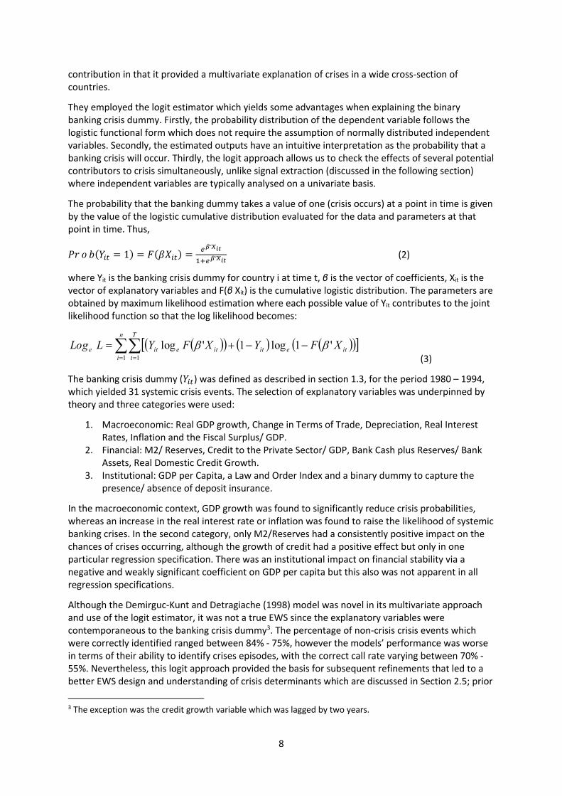
They employed the logit estimator which yields some advantages when explaining the binary banking crisis dummy. Firstly, the probability distribution of the dependent variable follows the logistic functional form which does not require the assumption of normally distributed independent variables. Secondly, the estimated outputs have an intuitive interpretation as the probability that a banking crisis will occur. Thirdly, the logit approach allows us to check the effects of several potential contributors to crisis simultaneously, unlike signal extraction (discussed in the following section) where independent variables are typically analysed on a univariate basis.

The probability that the banking dummy takes a value of one (crisis occurs) at a point in time is given by the value of the logistic cumulative distribution evaluated for the data and parameters at that point in time. Thus,

𝑃𝑟 𝑜 𝑏(𝑌+! = 1) = 𝐹(𝛽𝑋+!) =$!ʹ"#$

),$!ʹ"#$ (2)

where Yit is the banking crisis dummy for country i at time t, β is the vector of coefficients, Xit is the vector of explanatory variables and F(β Xit) is the cumulative logistic distribution. The parameters are obtained by maximum likelihood estimation where each possible value of Yit contributes to the joint likelihood function so that the log likelihood becomes:

(3)

The banking crisis dummy (𝑌+!) was defined as described in section 1.3, for the period 1980 – 1994, which yielded 31 systemic crisis events. The selection of explanatory variables was underpinned by theory and three categories were used:

1. Macroeconomic: Real GDP growth, Change in Terms of Trade, Depreciation, Real Interest Rates, Inflation and the Fiscal Surplus/ GDP.

2. Financial: M2/ Reserves, Credit to the Private Sector/ GDP, Bank Cash plus Reserves/ Bank Assets, Real Domestic Credit Growth.

3. Institutional: GDP per Capita, a Law and Order Index and a binary dummy to capture the presence/ absence of deposit insurance.

In the macroeconomic context, GDP growth was found to significantly reduce crisis probabilities, whereas an increase in the real interest rate or inflation was found to raise the likelihood of systemic banking crises. In the second category, only M2/Reserves had a consistently positive impact on the chances of crises occurring, although the growth of credit had a positive effect but only in one particular regression specification. There was an institutional impact on financial stability via a negative and weakly significant coefficient on GDP per capita but this also was not apparent in all regression specifications.

Although the Demirguc-Kunt and Detragiache (1998) model was novel in its multivariate approach and use of the logit estimator, it was not a true EWS since the explanatory variables were contemporaneous to the banking crisis dummy3. The percentage of non-crisis crisis events which were correctly identified ranged between 84% - 75%, however the models’ performance was worse in terms of their ability to identify crises episodes, with the correct call rate varying between 70% - 55%. Nevertheless, this logit approach provided the basis for subsequent refinements that led to a better EWS design and understanding of crisis determinants which are discussed in Section 2.5; prior

3 The exception was the credit growth variable which was lagged by two years.

( )( ) ( ) ( )( )[ ]åå= =

--+=n

i

T

titeititeite XFYXFYLLog

1 1'1log1'log bb

9

to this we discuss the Signal Extraction methodology which emerged around the same time as an alternative approach to crisis prediction.

15.2.3 Signal extraction (Kaminsky, and Reinhart (1999))

Kaminsky, and Reinhart (1999), pioneered the use of high frequency data in an event study analysis of financial crises. They specifically probed the occurrence of “twin crises” – namely events where currency crises are followed by banking crises, or vice versa. Using a dataset spanning the 1970s to 1990s, industrialised and developing countries, they captured both types of crises as follows: a banking crisis “event” started if either (i) bank runs led to the closure, merger or nationalisation of one or more financial institutions, or (ii) in the absence of bank runs, either one large bank or a group of banks were closed, merged or received large-scale government bailouts prior to similar measures undertaken on other financial institutions. Identification of these crisis events and their start dates relied on the extant banking crisis literature and financial press. Currency crises were dated using the high frequency exchange rate pressure index which was constructed as the weighted average of changes in exchange rates and central bank reserves, whereby the weights ensured the two variables had identical conditional volatilities. A currency crisis start date was then recorded if this variable exceeded three standard deviations from the mean.

In contrast to the Demirguc-Kunt and Detragiache (1998) logit model, the Kaminsky and Reinhart (1999) study provided a very different alternative to the investigation of crises. Whereas the logistic estimator is parametric, the signal extraction approach is non-parametric and falls under the broad category of event studies. Another difference is that it typically uses a univariate approach as opposed the multivariate models described above, although some studies have used combinations of variables as a single composite time series (Borio and Drehmann, 2002). Two major advantages of this methodology are that it is relatively easy to execute due to low computational requirements and because of the univariate nature, the data requirements are less burdensome.

The signal extraction approach is also intuitive in its interpretation: an indicator is tracked against a pre-defined threshold. The latter is chosen to discriminate between tranquil periods, where the indicator behaves according to a reasonable probability distribution and periods of crises where the variable displays an aberrant trend. Hence, whenever the variable value crosses the threshold, the model is effectively signalling a crisis and if the variable remains within the threshold boundary in any period, this corresponds to a non-crisis signal:

Let, i = a univariate indicator, j = a particular country, S= signal variable and X = indicator

An indicator variable relating to indicator i and country j is denoted by Xij and the threshold for this

indicator is denoted as X*ij A signal variable relating to indicator i and country j is denoted by: S i

j . This is constructed to be a binary variable where S i

j = {0,1}. If the variable crosses the threshold, a signal is emitted and S ij = 1. This happens when

{ S ij = 1 } = { │ Xij │ > │ X*i

j │ } (4)

If the indicator remains within its threshold boundary, it behaves normally and does not issue a signal so that S ij = 0,

{ S ij = 0 } = { │ Xij │ ≤ │ X*i

j │ } (5)

The threshold for each indicator is selected to minimise the NTSR, as described in equation (1). Note the variable S i

j = {0,1} is the forecasted banking crisis dummy. In order to assess the accuracy of the signal extraction prediction, S i

j, is compared against the occurrence of actual banking crisis events. Details on the latter have been described in section 1.3 and in the Kaminsky and Reinhart (1999) model, this was constructed using the Caprio and Klingebiel (1996) database, public information and stylised facts of crises chronology described in Kaminsky and Reinhart (1996).

10

One of the drawbacks of the signal extraction framework is the fact that each individual indicator is likely to possess a low informational content since crises are unlikely to be driven by anomalies in one variable alone. As a result, the correct identification of a banking crisis usually occurs only when several indicators cross their respective thresholds. Kaminsky and Reinhart (ibid) assessed 16 indicators (which captured the financial sector, external sector, real sector and fiscal position) and found that if less than 20% of these variables emitted a crisis signal, no actual banking crises would be identified. Even to correctly call 31% of the banking crises in their sample, 80-100% of their indicators would have to cross their respective thresholds. This may partially stem from the fact that the univariate approach fails to take into account the interactions between different sectors which often matter in the chronology of a crisis event. We now describe an alternative approach which accommodates these types of variable interdependencies.

15.2.4 Binary Recursive Trees

The Binary Recursive Tree (BRT) method is another non-parametric approach but unlike signal extraction, it assesses multiple indicators simultaneously. Moreover, it is particularly suited to financial crises investigations because of its ability to detect interactions between multiple explanatory variables which may be endogenous. Another advantage is that this technique is able to discover non-linear variable anomalies, making it especially useful for the analysis of different crisis events which may display several common vulnerabilities but are actually triggered by different factors.

This approach was applied by Ghosh and Ghosh (2003) in the context of currency crises, Duttagupta and Cashin (2008) who examined banking crises and Manasse et al (2003) in the investigation of sovereign debt crises. Davis, Liadze and Karim (2011) subsequently applied the BRT methodology to a larger banking crisis dataset and provide a detailed explanation of the estimator.

The intuition behind the BRT is as follows: a recursive algorithm is applied to a set of explanatory variable time series and the corresponding set of banking crisis events (i.e. the banking crisis dummy time series). The sample is split into an in-sample “training” dataset and an out-of-sample “test sample”. For each variable (Xi), the algorithm checks all values against all potential thresholds (Vi) to identify the best threshold value (Vi

*) that discriminates between crisis and non-crisis periods.

Each threshold for each variable generates a specific ratio of type I and II errors and the optimal threshold is that which minimises the sum of the two errors, although different error weightings can be applied according to user preferences. This generates a ranking of the variables’ predictive power with the “best” variable and its corresponding threshold forming the first “parent node” of the tree with observations lower than the threshold being placed on one side and others being places on the other side. This segregation rule is then recursively repeated until all variable observations are partitioned at different thresholds. A final tree may take the form as shown in figure 1, which then shows the pathway to each crisis with the corresponding variables of importance and their threshold values. The final tree is calibrated on the “training” dataset as an out-of-sample robustness exercise.

The output from the BRT methodology differs from the signal extraction and logit approaches in that it provides a context specific journey towards each crisis, showing the interactions of all the variables that culminate in banking system failure. By identifying the optimal thresholds, the model also provides policy makers with a monitoring benchmark so they can take preventive action if real time data suggests a threshold is being approached. The technique highlights that not all crises are the same and can thus be used to compare events between different economic structures such as developed versus developing economies or market based versus bank based financial systems.

There are however, certain disadvantages associated with the BRT approach. Firstly, the non-parametric estimation means confidence intervals are not attached to forecasts. Secondly, the recursive nature of the algorithm can lead to overfitting and as a result, trees can grow to become

11

extremely complex with little informational gain. It can also be argued that the complexity of the output is counterproductive from the policy makers’ perspective since she cannot monitor or influence every variable in a pathway without incurring significant economic disruption. These factors may explain why the BRT approach has not been widely adopted by regulators as part of their macroprudential monitoring and why the logit approach continues to be popular. We discuss recent refinements to the latter in the next section.

Source: Davis, Karim and Liadze (2011).

15.2.5 Second Generation Logit Models (Barrell et. al (2010))

Although the signal extraction and BRT approaches can provide useful insights into the causes of banking crises, their non-parametric nature has led to limited application in EWS design. In contrast, the logit estimator is a more accepted methodology in the extant literature and in this section, we outline some recent refinements to previous versions.

As described in Section 2.2, the Demirguc-Kunt and Detragiache (1998) model was not an EWS per se, in the sense that the explanatory and dependent variables were contemporaneous. Davis, Liadze and Karim (2011) analysed banking crises in Latin America and Asia and argued that lagged explanatory variables were necessary to avoid endogeneity between banking crises and the independent variables since the occurrence of a systemic crisis is likely to influence the behaviour of the explanatory variables. This was reinforced in Barrel et al. (2010) whose objective was to design an EWS that could explain and forecast the rash of OECD banking crises which manifested during the Sub-Prime episode.

Entire Sample: 72 crises

PARENT NODE

Child Node 2:

20 crises

Child Node 1:

52 crises

Terminal Node 3:

48 crises

Terminal Node 3:

4 crises

Terminal Node 4:

17 crises

Terminal Node 5:

3 crises

Splitter Variable: X1

X1≤ V1* X1>V1*

Splitter Variable: X2

X2≤ V2* X2> V2* X3≤ V3*

Figure 1: Schematic Diagram of Binary Recursive Tree (BRT)

X3≥ V3*

Splitter Variable: X3

12

The Barrell et al. (ibid) approach involved a sample of 14 banking crises in 14 OECD countries: Belgium, Canada, Denmark, Finland, France, Germany, Italy, Japan, Netherlands, Norway, Sweden, Spain, UK and the US. This country selection approach differed from previous studies where countries were often pooled despite the fact that there could be significant heterogeneity in their banking system characteristics and thus in the causes of crises (Davis, Liadze and Karim, 2011). Heterogeneous pooling was often used as an attempt to overcome the fact that systemic crises are historically relatively rare events and thereby increase the proportion of crisis observations in a sample. However, this approach could lead to EWSs that generated high type I and II errors and poor out-of-sample performance. Barrell et al (ibid) argued that good EWS design required pooling of countries that were broadly similar in terms of financial structure and economic development.

The sample period (1980 – 2007) was selected in order to add another innovation to the underlying Demirguc-Kunt and Detragiache (ibid) model. By restricting the start date to 1980, this allowed the authors to test bank specific macroprudential variables which had not been included in previous models due to lack of consistent historic time series data. The key additions included bank capital adequacy, narrow bank liquidity and property price growth since narratives on the sub-prime crises cited inadequate capital buffers and liquidity as problems in the face of increasingly risky mortgage lending.

Another refinement was the use of a general to specific approach. Barrell et al (ibid) argued that well designed EWSs should not only be robust but also parsimonious since they are designed to be practical tools to support the financial stability objectives of policy makers. While more complex and detailed econometric descriptions of crises may be informative, they may not identify a set of core variables that can be efficiently targeted as part of macroprudential policy. The general to specific approach may also lead to better performance in terms of lower type II error rates since variables that only explain a limited number of crises are eliminated, although a drawback could be a higher type I error rate as some idiosyncratic crises are not captured.

The use of lags combined with the general to specific approach and the inclusion of bank specific variables generated an EWS that differed substantially from the original Demirguc-Kunt and Detragiache (1998) model: the three core factors that explained the OECD crises were capital adequacy, liquidity and property price growth. This structure remained stable in the face of a series of robustness tests including country eliminations, alternative specifications of the banking crisis dummy, change of sample period and exclusion of post-crisis observations. The stability of the model supported the argument that EWS design should take into account the nature of the target economies and that models may need to be adapted periodically to reflect evolutions in banking systems and data availability.

15.2.6 Recent model comparisons and new techniques

Davis and Karim (op. cit.) comparing the logit and signalling approach, found that both models are useful, the signal model being better at predicting country-specific crises and the regression model more suitable for detecting global stress. In a recent “horse race” between 9 different approaches to crisis prediction in European countries (Alessi et al 2014) it was suggested that multivariate approaches have added value over simple signalling models, because although signalling was seen as transparent and straightforward, the risk of underestimating the probability of a crisis was high. Logit models may be sensitive to model specification while decision trees’ out-of-sample performance is little-known. Their recommendation of using a suite of models in policy is shown in practice by the ECB work in Section 3.2 below.

In another such “horse race”, Holopainen and Sarlin (2017) are more categorical in recommending machine learning approaches such as so-called k-nearest neighbours and neural networks, and particularly by model aggregation approaches through ensemble learning. In contrast, results of Beutel et al (2018) show that machine learning methods are not superior to conventional models in

13

predicting financial crises. In fact, the predictive performance of conventional models often exceeds that of machine learning methods considerably.

Multivariate models tested by Alessi et al (2014) had features such as addressing uncertainty, choosing indicators by Bayesian techniques and use of random coefficients to allow for cross country variation. Further developments include models with discrete choice over more than two states such as crisis, post crisis and tranquil (Bussiere and Fratzcher 2006). Tools based on artificial intelligence may offer some benefits but Alessi et al (2014) note that the input data has to be chosen by the user, and it is not always clear how risk patterns are detected. Recent work in this area includes the “random forest” of Alessi and Detken (2014), a machine learning methods based on decision trees, for detecting systemic risk.

Other recent work looks at alternative dependent variables to the standard banking crisis dummy. Boyd, De Nicolo and Loukoianova (2009) constructed two sets of systemic bank shock (SBS) indicators using aggregate bank balance sheet data. The first type of indicator focused on the asset side of banks’ balance sheets and captured anomalous declines in lending. In this case, the binary dummy became equal to one if real domestic lending growth in a given country fell below the 25th or 10th percentile of the real credit growth variable distribution across all countries in the sample. A similar process was used to create the second binary banking crisis variable which captured anomalies on the liability side of the balance sheet, namely the growth rate of the deposit-to-GDP ratio. These indicators had predictive power when introduced in lagged form into a logit EWS.

There is a burgeoning literature on the use of high frequency data to characterise financial stress which is extensively reviewed in Kliesen, Owyang, and Vermann (2012). Banking crisis dummies based on observed bank stress or policy responses are inherently backward looking and face criticism of subjectivity in terms of start dates (see below). It is argued that high frequency market data avoids this problem since asset prices should price in expectations of financial instability and its impact on the real economy. Hence, it is expected that anomalous values of these financial stress indicators should coincide with episodes of financial crises and therefore this approach provides an alternative left-hand side variable in EWSs. Typical market information that is embedded includes interest rate spreads on bonds (expected to capture higher rates of firm defaults in the event of crises), stock prices (which, via a dividend discount model are expected to capture lower future earnings), and exchange rates.

Babecky et al (2103) combine continuous (quarterly) information contained in output losses, employment rates and fiscal deficits and discrete (event based) banking crisis dummies. Vermeulen et al (2015) use the financial stress index approach to examine 28 OECD countries, although they find a weak relationship between their indicator and actual banking crisis episodes. Kliesen, Owyang, and Vermann (2012) compare the correlations of nine different financial stress indices in the US against National Bureau of Economic Research recession dates and find no significant relationship.

3 Looking Ahead: Usage of EWS in Policy Formation

This final section of the paper considers the usage of EWS as developed in the academic literature by policymakers, viewed in the overall context of their mandate to maintain financial stability.

15.3.1 Data requirements for EWS

The data needs for early warning systems as estimated in the academic literature and summarised in Section 2 are broadly as defined by the results. We note that these typically include a number of macroeconomic and macrofinancial variables. Recent developments have included the focus on aggregate banking sector variables as in Barrell et al (2010). A further development which has been widely neglected hitherto is the role of banking competition in raising the risk of financial crises, as in Davis et al (2020). As will be discussed further below, some institutions do indeed use binary estimated model outputs as part of their overall surveillance.

14

A key variable typically used in practice, not least given its prominence in Basel III and recommendation to be monitored as trigger for the countercyclical buffer, is the credit-to-GDP gap. This is as calculated by the BIS to be the difference between the actual total credit/GDP ratio and its trend as calculated by a Hodrick-Prescott filter (BCBS 2010). As summarised in Davis et al (2017), a range of studies have shown this indicator to be a useful indicator for financial crises, complementing binary choice models.

In a typical central bank or international organisation, the overall monitoring of vulnerability to financial instability in macroprudential surveillance, which is the function of EWS, goes much wider. Suggested lists of macroprudential indicators date back at least to Davis (1999) of the Bank of England and the IMF’s Financial Soundness Indicators. The origin of such lists includes not only the output of empirical studies but also the various academic theories of financial instability and the evidence drawn from actual crises – for example the Asian crisis showing risks of foreign currency exposures of the non-financial sectors.

In this context, it is suggested by Aikman et al (2015, 2017) of the Bank of England and the Fed that “no single data series is appropriate for gauging the build-up of risks in a complex and evolving financial system” (ibid, p36). Indeed, their own work highlights the potential role of 46 such indicators for the US, and show (Table 1 below) that this is a typical approach of a central bank or international organisation. They suggest that such indicators come appropriately in three categories – first, investor risk appetite and asset price indicators; second, nonfinancial sector leverage and related imbalances; and third, financial sector vulnerabilities linked to leverage, maturity transformation, wholesale funding and shadow banking.

Again following a typical central bank point of view, they critique the approach of relying on binary probability models given the infrequency of crises and consequent difficulty of highlighting a range of relevant factors. Rather, they focus on a range of indicators showing ability to forecast the credit cycle, highlight growing vulnerability and amplify shocks. They aggregate them in various ways to obtain overall measures of vulnerability. They find that the investor risk appetite leads the other groups of measures – and also the credit to GDP gap. But they acknowledge a need to supplement data with structural characteristics (what Davis (1999) calls qualitative information) like the run risk of money market funds. A similar analysis for the UK is given in Aikman et al (2018)

In this context, Aikman et al (2017) include a useful chart that shows the use of macroprudential data to monitor risks or to trigger policy decisions. The key points are that each institution does indeed employ a large number of indicators, that they often use summary illustrations of vulnerability such as heat maps, and that they do not generally make explicit reference to overall assessments of vulnerability.

Table 1: Use of macroprudential indicators by official institutions

15

Source: Aikman et al (2015)

15.3.2 Practical use of EWS

So what use is made of estimated EWS in practice? It would appear that for many institutions, research may proceed but use in “front line” surveillance is limited. That said, an exception would appear to be the ECB. In ECB (Constancio et al 2018), the quite extensive “analytical apparatus” is said to focus on three areas, first taking stock of the state of financial stress, second measuring the build-up of systemic instability and third development of macrofinancial models to assess the potential severity of a financial crisis.

Concerning the first group, taking stock of financial stress at present, the ECB highlight the probability of default by large and complex banking groups (an EWS called JPoD), the euro-area measure of systemic risk known as the Composite Financial Stress Indicator (CISS) and the corresponding Country Level Index of Financial Stress (CLIFS). They note that these are coincident indicators that do not help predict the near-term incidence of financial instability. This is rather generated by the Financial Stability Risk Index (FSRI) which as in the discussion above, combines 23 macrofinancial indicators (to capture time series risk) with 16 measures of spillover and contagion (cross-section risk). A first step is to filter out noise with four factors, a second is to recursively regress the four factors in a quantile regression on unexplained GDP components. The quantile

16

approach aims to capture nonlinearities around systemic events and focus in amplification mechanisms. Then forecast performance is evaluated with a goodness of fit measure.

Then as regards the second group measuring the build-up of systemic instability, the focus is on prediction of instability at a usable policy horizon of 2-3 years, again looking both at cross-section and time series levels. Measurement of financial cycles at a country and Eurozone level – as distinct from the business cycle which is much shorter and with a lower amplitude - uses measured based on credit and house prices for a “narrow” measure and then also equity and bond prices at a “broad” level. It is suggested that such composite financial cycle indicators are the best indicators of the start of systemic banking crises and periods of vulnerability, superior to the credit-to-GDP gap for example.

Early warning models are also part of the ECBs armoury and indeed are “a key element of the analytical apparatus supporting macroprudential policy decision making” (ibid, p37). That said, they note at least three important problems with use of EWS in policy decisions. First, structural breaks may make the signal less effective. Second, there are differences between Eurozone countries’ financial sectors meaning models require careful interpretation. And third, there could be a difficulty like Goodhart’s Law that the use of use of early warning models for macroprudential policy may blur the future relation between the indicator and crises. The importance of testing out-of-sample is also emphasised.

Five approaches are used, as identified in Section 2, namely univariate and bivariate signalling models, a multivariate logit early warning model at the country level, a multivariate logit early warning model using individual bank level data, a random forest, and aggregate risk indicators derived from risk scoreboards. As shown in Table 2, a Markov switching model is also employed.

In terms of presentation, for the signalling approach there could be columns for each variable showing the estimated crisis probability for each country (see ibid p39) such as residential property price overvaluation but also the illustration of different crisis thresholds and summary conditional crisis probabilities (we discuss these issues further in the following section). This presentation is similar for the multivariate estimates, examples of which are shown in Table 2. The different models evidently differ in their intensities of warning signals and the art of surveillance is to interpret them appropriately and deliver useful judgement to decision makers.

The final measure in this group the cyclical systemic risk indicator (CSRI) based on a scoreboard which seeks to summarise the individual EWS measures whereby “early warning properties or expert judgement are used to select six to ten indicators per risk category, ideally covering different types of vulnerability. The individual indicators are then aggregated into one summary systemic risk indicator where the weights are determined to optimise the in-sample and out-of-sample early warning performance.” (ibid, p41). This measure is considered to signal accurately the likelihood and severity of crises as it includes both domestic and exposure based SRIs.

17

Table 2: Identified vulnerabilities based on selected multivariate early earning models.

Source: Constancio et al (2018)

The final tool highlighted by the ECB is the macroprudential stress testing apparatus STAMP€, a form of macrofinancial model usable both to assess the impact of given risks on banking sectors and also to consider the effect of policy measures.

The approach of the ECB typifies that of an advanced country or area which has ample research resources and related access to long runs of consistent data. The World Bank (Krishnamurti and Lee, 2014) offers a useful counterpoint for developing and emerging countries. It is suggested that for them an EWS needs to be useable for monitoring build-ups of risk, analysing the signals of risk build-up, interpreting the signals, assessing overall vulnerability, identifying a need for a policy response and communicating warnings and assessments for backing such a response.

Such an approach needs to start at a basic level of ensuring that surveillance covers all relevant financial institutions and markets. Then there is a need for early detection of systemic risk, with the caution that crisis prediction is an inexact art. An EWS, it is suggested can at best detect a build-up of vulnerabilities but not the feedback effects within the financial system and vis a vis the real sector. And data to build indicators are likely to be scarce in developing countries. Hence again rather than model building it is recommended that the macroprudential authority seek to identify and monitor leading indicators of financial instability. Aggregation as a composite measure is also recommended. The set of indicators should include non-banking measures both across and outside the financial system (this is a criticism of the IMFs initial set of financial soundness indicators that they focused

18

too much in the banking sector). The World Bank also mention qualitative trends relevant to financial stability that are not captured by models such as financial innovations, new products, changes in banks’ business models, the type of model used by market participants and the risk of regulatory arbitrage. To provide a forward looking element, stress tests and scenario analyses are recommended.

The World Bank suggest that many countries with limited resources and data should rely on a small number of EWIs whose risk properties are understood and where there are staff resources to analyse them. Then there is a need to identify warning thresholds which trigger a need for policy concern and then trigger thresholds for the introduction of macroprudential policy measures. There is a need to communicate results specifically and sufficiently early for the policy measures to have an effect. The World Bank note that while external communication is vital, publishing a Financial Stability Review is not a guarantee of protection. Cihak et al (2011) found 80 countries publishing FSRs at that time but little evidence of a direct link to financial stability, unless there were high quality publications with forward looking elements. Data gaps, lack of skilled personnel and poor quality modelling may all vitiate efforts.

Meanwhile, IMF (2013) in its major policy paper on macroprudential policy, suggests in terms of surveillance that “tools exist to assess most sectors and levels of aggregation. However, these tools provide only partial coverage of potential risks and only tentative signals on the likelihood and impact of systemic risk events. As such, they may not provide sufficient comfort to policymakers.”

15.3.3 Incorporating policymakers’ preferences

As noted above and as shown in Table 2, there is scope with estimated EWS to incorporate relevant information for policymakers beyond the simple probability of a crisis which is generated by the respective model. Policymakers require an EWS not only to have good forecasting power but also give an early enough signal and be stable. The signal needs to be early enough for macroprudential policies to take effect but also not too early as this would impose unnecessary costs on the economy – and pressure to weaken future policy actions. The signal also needs to be stable since policymakers prefer to react to persistent rather than temporary signals, since this reduces uncertainty over the actual state of the economy and allows for more decisive policy action. The signal should also be robust to sample changes and easy to interpret.

In this context there needs to be allowance for the policymaker’s preference over Type I error (failing to forecast a crisis that does occur) and Type II error (forecasting crises when they do not occur). Drehmann and Juselius (2014) offer an approach to this issue, incorporating the policy requirements cited above, aspects of which are followed in many recent papers providing estimated EWS. A key issue is to evaluate the quality of signals in the absence of knowledge of the costs and benefits of policy actions. In particular, they highlight the receiver operating characteristic curve (ROC) which, as noted above, maps the full range of trade-offs of Type I and Type II error that the EWS provides. It does this by mapping the false positive rate (Type II error) to the true positive rate (complement of Type I error). They contend that the area under the curve (AUROC) is a helpful summary measure of the signalling quality of the EWS. There is scope to compare the AUROC of two alternative EWS by for example confidence bands and Wald statistics.

Drehmann and Juselius (2014) evaluate the signalling properties of 10 EWS using these AUROCs around the time of crises and find the debt service ratio (over shorter horizons) and the credit-to-GDP gap (over longer horizons) perform best. Evaluations based on them are indeed robust over a range of policymaker preferences, they are well timed and the quality does not deteriorate in the run-up to the crisis. Other indicators often have signalling qualities that vary sharply over time.

Rereading Table 2 we can see that the AUROC is shown for each of the EWS shown. A perfect prediction would give an AUROC of 1.0 while an uninformative mode would have one of 0.5, the

19

closer to unity the better (Filippopolou et al 2020). There is also information for those willing to accept different levels of probability of a crisis with signalling thresholds between 0.3 and 0.7, and associated Type I error rates (T1) and Type II error rates (T2) as well as the conditional probability of a crisis (CP). Those most concerned about a crisis would choose 0.7 and those most concerned to avoid over prediction would choose 0.3.

3.4 Use of macroprudential surveillance (EWS) to trigger macroprudential policy action

The Bank of England approach to adjusting the countercyclical buffer gives a good example of the use of risk assessments and early warning indicators to guide decision making (Aikman, Haldane and Kapadia 2013). Constancio et al (2018, 51-53) show the equivalent process for the ECB. Aikman et al point out that “given the complexity and state-contingency of signals from indicators and models, it would not make sense to tie movements in the CCB mechanically to any specific set of indicators or models” (ibid p18). Rather, use is made of a short list of core financial and economic indicators, which are thought useful inter alia to anchor policy actions, give consistent decision making and a basis for explain actions externally. Interestingly, it is suggested that simple indicators can outperform in terms of prediction more complex approaches due to their robustness in the face of uncertainty.

The credit to GDP gap is indeed used as a starting point but it has to be supplemented due to weaknesses such as the poor ability to signal in deteriorating conditions, ignoring absolute amounts of credit and their sources and quality (Giese et al 2014). Additional indicators include aggregate risk adjusted capital and leverage ratios (as tested globally in Davis et al 2020), the loan to deposit ratio as a measure of dependence on wholesale funding, low quality debt spreads, banks’ price to book ratios and market value capital ratios, the current account deficit, ad global capital market measures such as the VIX, global spreads and long term interest rates.

It is emphasised that stress tests and output of other models as well as market intelligence are also an input to the decision in the Financial Stability Committee. That is then promulgated via a press release, the meeting minutes and the biannual FSR. International coordination takes place under Basel rules to ensure international banks’ exposure to the UK are also subject to the CCB. Banks have 12 months to apply an increase in the CCB, a lag that needs to be taken into account in policy making. It is finally noted that although there are some calculations of the effect of CCB increases on prices and quantities of credit, and on GDP, these were limited at the time of writing.

3.5 Interaction of EWS with monetary policy rules

The interaction of macroprudential and monetary policy is an open question which is very important to macroprudential policy and the usage of EWS. Svensson (2018) argues that monetary policy has a strong effect on price stability and real stability but a small, indirect and unsystematic effect on financial stability, while macroprudential policy has a strong effect on financial stability but a small indirect and unsystematic effect on inflation and resource utilisation.

Accordingly, he argues that the policies are best directed to separate goals – price and real stability for monetary policy and financial stability (ability of the financial system to fulfil its functions with sufficient resilience to disturbances that threaten these functions) for macroprudential policy. Thus, these policies can be best undertaken separately, while taking account of the likely action of the other, as in a Nash equilibrium. Such separate conduct helps both policies to be distinct, transparent and easy to evaluate and hence facilitates accountability for the decision making body in achieving the relevant goals. A similar argument can be made for separate monetary and fiscal policy.

The implication for macroprudential surveillance and EWS is that they should take into account an expected path of monetary policy that seeks to maintain monetary stability but is not adjusted to also combat financial instability. The same applies to “inflation reports” and other input to monetary policy decisions in respect of anticipated macroprudential policy decisions. Svensson argues that

20

monetary policy should not seek to target financial stability, which it is not capable to achieve; he discounts the “risk taking channel” of monetary policy that some argue requires it to have a financial stability as well as monetary stability focus (Adrian and Liang 2018).

Svensson suggests that the main exception to this optimal separation is in a crisis episode per se when both policies along with fiscal policy need to work to return the economy and financial system to balance. He argues strongly against monetary policy seeking to aid macroprudential policy by “leaning into the wind” and raising rates above those warranted by monetary stability to aid financial stability, suggesting this policy can have few benefits and major costs – notably a weaker economy with lower inflation and higher unemployment if there is no crisis, and a higher cost of crisis if one does occur. The only other exception to the Nash equilibrium, he argues, should be when the macroprudential authorities themselves ask for help from the monetary authorities on the basis that they cannot maintain financial stability with their own instruments.

Such a stance is not without critics, in particular BIS economists such as Juselius et al (2016) have argued for close coordination and leaning into the wind when it is appropriate. And empirical work such as Kim and Mehrota (2018) for four Asia-Pacific economies that have inflation targets (Australia, Korea, Thailand, Indonesia) shows that the macroeconomic effect of monetary and macroprudential policy is in fact quite comparable, since both lead to reallocation of spending over time by influencing the availability and cost of credit. For contractionary policies of either type there is a decline in GDP, the price level and the stock of credit They argue accordingly that whereas most of the time monetary and macroprudential policy can operate alongside each other in a beneficial way, there could be important conflicts in the case that there is low inflation and buoyant credit growth. In such cases an EWS needs to consider not only direct risks to financial stability but also the effects of variations of monetary policy from direct targeting of inflation and forms of coordination may be necessary.

Complementing these are a wide range of theoretical papers that seek to trace the interrelation of monetary and macroprudential policy. To give one example, Agur and Demertzis (2015), using a bank-based model (profitability and leverage), saw that with the presence of macroprudential policy, there is at times a partial offsetting of monetary policy (expansionary interest rate policy) and at the same time, monetary policy can affect financial stability (e.g. the Latin debt crisis of the early 1980s and loose monetary policy in the 2000s leading up to the subprime crisis).

3.6 Some open issues with EWS

Other open issues include (Aikman, Haldane and Kapadia 2013) the effect of macroprudential policy in a downturn and calibration in the context of uncertainty. There is a need to consider whether policy and surveillance are too narrowly focused on the banking system and whether tools addressing market and non-bank finance are needed (Constancio et al 2018). There is the issue whether there should be targeting of asset prices such as house prices by macroprudential policy (Constancio 2016). Measurement and control of policy leakages due to regulatory arbitrage within banks, across the financial system and offshore needs more attention.

The issue of shadow banking requires close attention in terms of monitoring and assessing risks, including appropriate monitoring and use of EWS. Then, as discussed in Section 2.6, there is the utility or otherwise of machine learning approaches to crises, which remains an open issue. Finally, we note that our own work suggests inter alia a need to focus on the relation of measures of banking competition to crises and use of both leverage ratios and risk adjusted capital in EWS. We also suggest a need to allow for nonlinear relations between capital and crises (Davis et al 2020).

21

REFERENCES

Adrian T, and Liang N (2018) “Monetary policy, financial conditions, and financial stability,” International Journal of Central Banking 14(1), 73–131

Agur I, and Demertzis M (2015), “Will Macroprudential Policy Counteract Monetary Policy’s Effects on Financial Stability?”, IMF Working Paper, 15/283.

Aikman D, Bridges J, Burgess S, Galletly R, Levina I, O’Neill C and Varadi A (2018) “Measuring risks to UK financial stability”, Bank of England Staff Working Paper No. 738

Aikman D, Haldane A G and Kapadia S (2013), “Operationalising a macroprudential regime, goals, tools and open issues”, Bank of Spain Working Paper 24

Aikman D, Kiley M, Lee S J, Palumbo M G and Warusawitharana M (2015), “Mapping heat in the US financial system”, Finance and Economics Discussion Paper Series 2015-019, Board of Governors of the Federal Reserve, Washington DC

Aikman D, Kiley M, Lee S J, Palumbo M G and Warusawitharana M (2017), “Mapping heat in the US financial system”, Journal of Banking and Finance, 81, 36-64

Alessi L, Antunes A, Babecky J, Baltussen S, Behn M, Bonfim D, Bush O, Detken C, Frost J, Guimaraes R, Havranek T, Joy M, Kauko K, Mateju J, Monteiro N, Neudorfer B, Peltonen T, Rodrigues P, Rusnák M, Schudel W, Sigmund M, Stremmel H, Smidkova K, van Tilburg R, Vasicek B and Zigraiova D, (2014) “Comparing different early warning systems: Results from a horse race competition among members of the macro-prudential research network”. ECB, mimeo

Alessi L and Detken C, (2014) “Identifying excessive credit growth and leverage”. ECB Working Paper No. 1723

Babecký J, Havránek T, Matějů J, Rusnák M, Šmídková K and Vašíček B (2013), “Leading indicators of crisis incidence: Evidence from developed countries”, Journal of International Money and Finance, 35, C, 1-19.

Bank for International Settlements (1986), “Recent innovations in international banking, report prepared by a study group established by the central banks of the G10 countries”, Basel, April (Cross Report).

Barrell R, Karim D and Macchiarelli C, (2020)”Towards an understanding of credit cycles: do all credit booms cause crises?”, The European Journal of Finance, 26:10, 978-993.

Barrell R, Davis E P, Karim D, and Liadze I, (2010). “Bank regulation, property prices and early warning systems for banking crises in OECD countries”. Journal of Banking and Finance, 34, 2255-2264

Barrell R, Karim D, and Ventouri A (2016) "Interest Rate Liberalization and Capital Adequacy in Models of Financial Crises", Journal of Financial Stability, Volume 33, December 2017, Pages 261-272.

Basel Committee on Banking Supervision (2010), “Guidance for national authorities operating the countercyclical capital buffer”, BCBS, Basel

Beutel J, List S and von Schweinitz G (2018) “An evaluation of early warning models for systemic banking crises: Does machine learning improve predictions?” Deutsche Bundesbank Discussion Paper No 48/2018

BIS (1997a), 67th Annual Report, Basel, June

22

BIS (1997b), Survey of disclosures about trading and derivatives activities of banks and securities firms, Basel, November.

Borio, C and Lowe, P (2002). “Assessing the Risk of Banking Crisis”, BIS Quarterly Review, December 2002.

Boyd J H. and Gertler M (1993). “U.S. Commercial Banking: Trends, Cycles, and Policy”, NBER Chapters, in: NBER Macroeconomics Annual 1993, Volume 8, pages 319-377, National Bureau of Economic Research, Inc

Boyd J H, De Nicolo G and Loukoianova E, (2009) “Banking Crises and Crisis Dating: Theory and Evidence”, IMF Working Paper No. 09/141.

Bussière M. and Fratzscher M., (2006) “Towards a new early warning system of financial crises”. Journal of International Money and Finance, 25(6), 953–973.

Calvo G A. and Mendoza E G. (1996), “Mexico's balance-of-payments crisis: a chronicle of a death foretold”, Journal of International Economics, 41, 235-264.

Caprio G and Klingebiel D (1996), “Bank Insolvencies: Cross-Country Experience”, Policy Research Working Paper PRWP1620, Washington, D.C.: World Bank.

Caprio G and Klingebiel D (1999), “Episodes of Systemic and Borderline Financial Crises”, Washington, D.C.: World Bank Mimeo.

Caprio G and Klingebiel D (2003) “Episodes of Systemic and Borderline Financial Crises” In: Klingebiel, D., Ed., The World Bank, Washington DC

Caprio, Gerard, Daniela Klingebiel, Luc Laeven, and Guillermo Noguera, 2005, “Appendix: Banking Crisis Database,” in Patrick Honohan and Luc Laeven (eds.), Systemic Financial Crises: Containment and Resolution. Cambridge, U.K.: Cambridge University Press.

Čihák M, (2006), “How Do Central Banks Write on Financial Stability?", IMF Working Paper No. 06/163.

Čihák M, Muñoz S, Sharifuddin S T, and Tintchev K. (2012) “Financial Stability Reports: What Are They Good For?” IMF Working Paper No. 12/1.

Clement P, (2010). “The Term 'Macroprudential': Origins and Evolution”. BIS Quarterly Review, January 2010, 59-67.

Constâncio, V. (2016), “Principles of Macroprudential Policy”, speech given at the ECB-IMF Conference on Macroprudential Policy, Frankfurt am Main, 26 April 2016.

Constâncio V, Cabral I, Detken C, Fell J, Henry J, Hiebert P, Kapadia S, Altimari S N, Pires F, SalleoC (2018), “Macroprudential policy at the ECB: Institutional framework, strategy, analytical tools and policies”, ECB Occasional Paper 227

Davis E P (1995), “Debt, financial fragility and systemic risk”, Oxford University Press

Davis E P (1999), "Financial data needs for macroprudential surveillance: what are the key indicators of risk to domestic financial stability?", Lecture Series No 2, Centre for Central Banking Studies, Bank of England.

Davis, E P and Karim, D, (2008), “Comparing early warning systems for banking crises”, Journal of Financial Stability, 4, 89-120

Davis E P, Karim D, and Liadze I, (2011), “Should Multivariate Early Warning Systems for Banking Crises Pool across Regions?”, Review of World Economics / Weltwirtschaftliches Archiv 147, 693-716

23

Davis, E P, Karim D and Noel D (2017) “Macroprudential policy and financial imbalances”.Brunel Economics and Finance Working Paper 17-22

Davis E P, Karim D and Noel D (2020), “The bank capital-competition-risk nexus, a global perspective”, Journal of International Financial Markets, Institutions and Money, 65

Demirgüç-Kunt, A., Detragiache, E., (1998) “The determinants of banking crises in developing and developed countries” IMF Staff Papers 45 (1).

Demirgüç-Kunt A and Detragiache E, (2002), “Does Deposit Insurance Increase Banking System Stability? An Empirical Investigation”, Journal of Monetary Economics, 49, 1373-1406.

Demirgüç-Kunt A and Detragiache E (2005), “Cross-Country Empirical Studies of Systemic Bank Distress: A Survey”, National Institute of Economic Review, no.192, April,

Drees B and Pazarbasioglu C, “The Nordic Banking Crises: Pitfalls in Financial Liberalization?”, IMF Working Paper No. 95/61

Drehmann M and Juselius M (2014), “Evaluating early warning indicators of banking crises, satisfying policy requirements”, International Journal of Forecasting, 30, 759-780

Filippopoulou C, Galariotis E and Spyrou S (2020), “An early warning system for predicting systemic banking crises in the Eurozone, a logit regression analysis”, Journal of Economic Behaviour and Organisation, 172, 344-363

Gavin M and Hausmann R, (1998), “The Roots of Banking Crises: The Macroeconomic Context”. IDB Working Paper No. 262.

Ghosh S and Ghosh A R, (2002). "Structural Vulnerabilities and Currency Crises". IMF Working Paper No. 02/9, International Monetary Fund.

Giese J, Andersen H, Bush O, Castro C, Farag F and Kapadia S (2014) “The credit-to-GDP gap and complementary indicators for macroprudential policy: evidence from the UK”, International Journal of Finance and Economics, 19: 25–47

Holopainen M. and Sarlin P (2017). “Toward Robust Early-Warning Models: A Horse Race, Ensembles and Model Uncertainty”, Quantitative Finance 17 (12), 1-31.

IMF (1998), “Towards a Framework for Financial Stability”, World Economic and Financial Surveys, IMF Washington DC.

IMF (2013), “Key aspects of macroprudential policy”, IMF, Washington DC.

Juselius M, Borio C, Disyatat P and Drehmann M (2016), “Monetary policy, the financial cycle and ultra-low interest rates”, Bank for International Settlements Working Paper No. 569.

Kaminsky G L, and Reinhart C M (1996), “The twin crises: the causes of banking and balance-of-payments problems”, International Finance Discussion Papers 544, Board of Governors of the Federal Reserve System (U.S.), revised 1996.

Kaminsky G L, and Reinhart C M ,(1999), “The Twin Crises: The Causes of Banking and Balance-of-Payments Problems”, American Economic Review, 89 (3): 473-500.

Kim S and Mehrotra A (2018), “Effects of monetary and macroprudential polciies, evidence from four inflation targeting countries”, Journal of Money Credit and Banking, 50, 967-992

Kliesen K, Owyang M and Vermann E (2012). “Disentangling Diverse Measures: A Survey of Financial Stress Indexes”. Federal Reserve Bank of St. Louis Review. 94. 369-398.

24

Krishnamurti D and Lee Y C (2014), “Macroprudential policy, a practice guide”, World Bank, Washington D C

Laeven L and Valencia F, (2008), “Systemic Banking Crises: A New Database”, IMF Working Paper No. 08/224.

Laeven L, and Valencia F, (2013), “Systemic Banking Crises Database”, IMF Economic Review, 61 225–270.

Laeven L and Valencia F, (2018), “Systemic Banking Crises Revisited”, IMF Working Paper No 18/206

Li X, Escalante C L and Epperson J E (2014) “Agricultural Banking and Bank Failures of the Late 2000s Financial Crisis: A Survival Analysis Using Cox Proportional Hazard Model” Selected Paper prepared for presentation at the Southern Agricultural Economics Association(SAEA) Annual Meeting, Dallas, Texas, 1-4 February 2014

Manasse, P., Roubini, N., & Schimmelpfennig, A. (2003). “Predicting sovereign debt crises”, IMF Working Paper No. 03/221.

Pill, Huw R. and Pradhan, Mahmood, (1995). Financial Indicators and Financial Change in Africa and Asia, IMF Working Paper No. 95/123.

Schularick M. and Taylor A. (2012). “Credit booms gone bust: monetary policy, leverage cycles and financial crises, 1870–2008”, American Economic Review, 102, 1029–61

Svensson L E O, (2018), “Monetary policy and macroprudential policy; different but separate?”, Canadian Journal of Economics, 18, 802-827

Velasco, A (1987), Financial crises and balance of payments crises: A simple model of the southern cone experience, Journal of Development Economics, 27, 263-283

Vermeulen, R., Hoeberichts, M., Vašíček, B. et al. Financial Stress Indices and Financial Crises. Open Econ Rev 26, 383–406 (2015).

World Bank (2017), “Global Financial Development Database”, IBRD, Washington DC, http://www.worldbank.org/en/publication/gfdr/data/global-financial-development-database