E01426_MPCT_User's Manual.pdf
86
Didacta Italia MPCT Modular Process Control Trainer User’s Manual and Exercise Guide
-
Upload
danilo-jose-semprun -
Category
Documents
-
view
49 -
download
2
Transcript of E01426_MPCT_User's Manual.pdf
Didacta Italia
MPCT
Modular Process Control Trainer
User’s Manual
and Exercise Guide

Didacta Italia
MPCT
Modular Process Control Trainer
User’s Manual
and Exercise Guide
This manual illustrates the technical characteristics and operating instructions of the system Didacta MPCT Modular Process Control Trainer, giving the instructor or the student a specific knowledge of the unit and its applications. Besides the manual contains a choice of exercises ready to be performed in the laboratory.
Didacta Italia Srl - Strada del Cascinotto, 139/30 - 10156 Torino
Tel. +39 011 273.17.08 273.18.23 - Fax +39 011 273.30.88
http://www.didacta.it - e-mail: [email protected]
The information contained in this manual has been selected and verified with the
greatest care. However, no responsibility stemming from its use can be ascribed to the
Authors or to Didacta Italia or any person or company involved in its preparation.
The information contained in this manual can be modified at any time and without
warning on account of technical or educational needs.
Copyright Didacta Italia 2012
Reproduction by any means, including photocopying of this test or parts thereof, or the
figures contained therein, is strictly prohibited.
Printed in Italy — 30/03/12
Code 01426E0312 — Edition 01 - Revision 02
table of contents
MPCT - User’s Manual v
Table of Contents
1. General ..................................................................................... 1
2. System composition and description .................................... 3
2.1 Composition ............................................................................................... 3
2.2 Description ................................................................................................. 5
2.2.1 Electrical equipment .................................................................................................... 5
2.2.2 Process simulator ........................................................................................................10
3. Description of the control processes and techniques ....... 17
3.1 Level control ............................................................................................ 17
3.1.1 Process description ..................................................................................................... 17
3.1.2 Control techniques ..................................................................................................... 17
3.2 Flow control .............................................................................................. 25
3.2.1 Process description ..................................................................................................... 25
3.2.2 Control techniques ..................................................................................................... 25
3.3 Pressure control ....................................................................................... 26
3.3.1 Process description ..................................................................................................... 26
3.3.2 Control techniques ..................................................................................................... 26
3.4 Temperature control ............................................................................... 27
3.4.1 Process description ..................................................................................................... 27
3.4.2 Control techniques ..................................................................................................... 27
3.5 pH and conductivity control ................................................................. 28
3.5.1 Process description ..................................................................................................... 28
3.5.2 Control techniques .....................................................................................................30
4. Installation and preliminary operations .............................. 31
4.1 Level control ............................................................................................ 31
4.2 Flow control .............................................................................................. 33
4.3 Pressure control ....................................................................................... 35
4.4 Temperature control ............................................................................... 38
4.5 pH and conductivity control ................................................................. 40
table of contents
vi Didacta Italia
5. Exercises ................................................................................. 45
5.1 Exercise 1 — On-Off level control via software ...................................... 45
5.2 Exercise 2 — PID level control via software ............................................ 48
5.3 Exercise 3 — PID level control with MiniReg controller ......................... 53
5.4 Exercise 4 — PID flow control via software ............................................. 57
5.5 Exercise 5 — PID pressure control via software ...................................... 61
5.6 Exercise 6 — PID temperature control via software ............................. 65
5.7 Exercise 7 — On-Off pH/conductivity control via software ................. 69
5.8 Exercise 8 — PID pH/conductivity control via software ........................ 72
5.9 Exercise 9 — PID pH/Conductivity control with the MiniReg ............... 76
Chapter 1.
MPCT - User’s Manual 1/80
1. General
The MPCT system is a tool for the study of closed loop physical quantity control techniques.
In an industrial setting, this quantity will often be the level of liquid in tank, the pressure of a gas in a container, the temperature of a fluid, the flow of a liquid in a pipe.
The MPCT modular system makes it possible to test the control processes used for these four quantities.
The basic module is comprised of the electrical equipment, general purpose components and specific level control components.
Options include kids of additional components to control each of the following quantities: flow, pressure, temperature, pH, conductivity.
The transition from one process to another is quick an easy: it only requires making a few connections with silicone tubelets.
In general, the control action can be defined as follows:
to keep constant a physical quantity, referred to as controlled quantity (Y), being affected by an independent variable, referred to as noise (n).
The reference signal that we want to obtain for the controlled quantity is called set-point (SP) signal.
An “automatic” solution to the problem suggests the construction of a controller that is able to affect the controlled quantity through a control signal (x).
For instance, in level control, the issue to be addressed is to keep the level of a liquid in a tank constant when some of the liquid is drawn from the tank by a device that works independently.
The controlled quantity is the level of the liquid in the tank; the independent variable (noise) is the liquid leaving the tank (the volume of water “used up” in unit time).
The controller works by adjusting liquid inflow (the water volume “generated” in unit time).
The MPCT system uses a first pump to adjust the inflow and another pump to change the outflow.
The first pump is controlled by the control signal and the other by the noise signal.
The pressure exercised by the liquid onto the bottom of the tank being proportional to the liquid level in the tank, the controlled quantity is supplied to the controller by a pressure transducer.
General
2/80 Didacta Italia
The same scheme applies to the other cases (flow, pressure, temperature), but needless to say a different transducer is used.
The MPCT system makes it possible to set up and study digital and analog electronic control systems.
The control action, in fact, can be accomplished in the following ways:
• through the CRS (Control Regulation Software) software and a Personal Computer;
• through an electronic controller (e.g., the MiniReg electronic controller available as an option).
In the former case, the CRS accomplishes a digital control action, enabling the user to define the relative parameters and to observe the evolution of the various quantities involved in the process.
In the latter case, the software running on a Personal Computer (CRS) makes it possible to monitor the control action accomplished by the electronic controller and to transmit the set-point signal to said controller.
In either case, the software also makes it possible to control the action of the peristaltic pump (2) and hence to introduce noises of various types into the process.
The signal corresponding to the controlled quantity is acquired through the A/D (analog/digital) conversion of the signal supplied by the transducers. The control signal is acquired in the same manner when an external electronic controller is used.
The generation of the control signal (in the former case), that of the remote Set-Point signal (in the latter case), and that of the noise signal (in either case) is through a digital/analog (D/A) conversion of the digital signal processed by the software.
The aforementioned A/D and D/A conversion processes are performed by a single AD/DA card supplied as standard with the basic module of the MPCT system.
In the former case, the control action by the CRS software is either On-Off or PID (Proportional Integral Derivative). Controller parameters may be changed and their effects may be determined quickly and easily, enabling the students to become thoroughly familiar with these control techniques.
Moreover, since the “system” is made up of components as are normally used in industrial applications, its use leads to extensive knowledge of real and widespread problems.
We recommend reading the “Control Theory Basics” manual to learn the indispensable basic notions, and the CRS software manual before starting the tests with the unit.
Chapter 2.
MPCT - User’s Manual 3/80
2. System composition and description
2.1 Composition
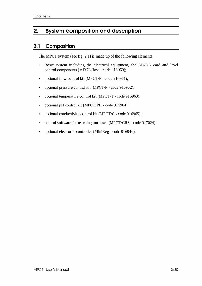
The MPCT system (see fig. 2.1) is made up of the following elements:
• Basic system including the electrical equipment, the AD/DA card and level control components (MPCT/Base - code 916960);
• optional flow control kit (MPCT/F - code 916961);
• optional pressure control kit (MPCT/P - code 916962);
• optional temperature control kit (MPCT/T - code 916963);
• optional pH control kit (MPCT/PH - code 916964);
• optional conductivity control kit (MPCT/C - code 916965);
• control software for teaching purposes (MPCT/CRS - code 917024);
• optional electronic controller (MiniReg - code 916940).
System composition and description
4/80 Didacta Italia
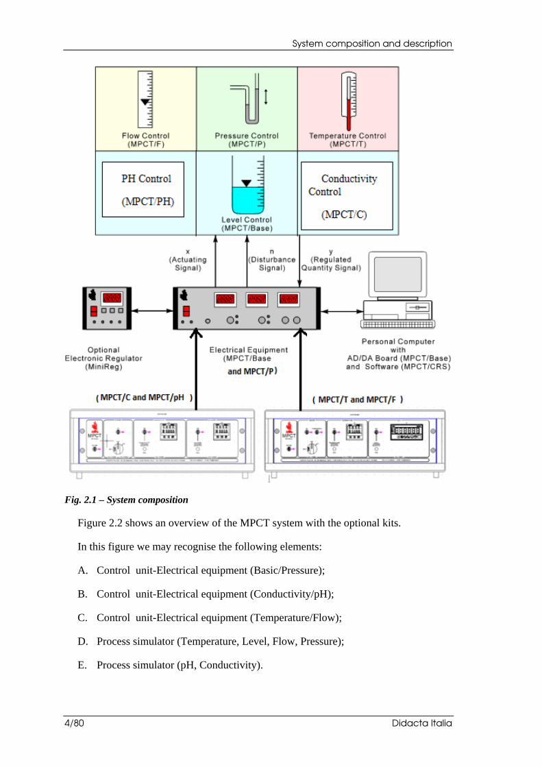
Fig. 2.1 – System composition
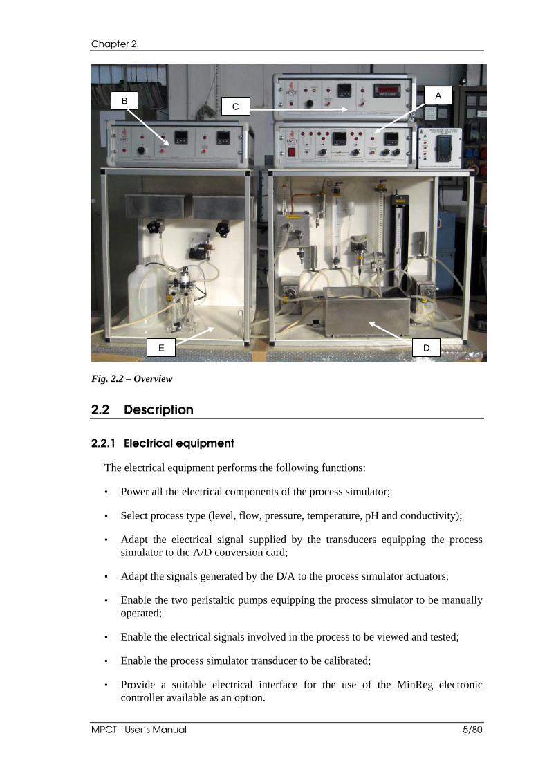
Figure 2.2 shows an overview of the MPCT system with the optional kits.
In this figure we may recognise the following elements:
A. Control unit-Electrical equipment (Basic/Pressure);
B. Control unit-Electrical equipment (Conductivity/pH);
C. Control unit-Electrical equipment (Temperature/Flow);
D. Process simulator (Temperature, Level, Flow, Pressure);
E. Process simulator (pH, Conductivity).
Chapter 2.
MPCT - User’s Manual 5/80
Fig. 2.2 – Overview
2.2 Description
2.2.1 Electrical equipment
The electrical equipment performs the following functions:
• Power all the electrical components of the process simulator;
• Select process type (level, flow, pressure, temperature, pH and conductivity);
• Adapt the electrical signal supplied by the transducers equipping the process simulator to the A/D conversion card;
• Adapt the signals generated by the D/A to the process simulator actuators;
• Enable the two peristaltic pumps equipping the process simulator to be manually operated;
• Enable the electrical signals involved in the process to be viewed and tested;
• Enable the process simulator transducer to be calibrated;
• Provide a suitable electrical interface for the use of the MinReg electronic controller available as an option.
C B
A
D E
System composition and description
6/80 Didacta Italia
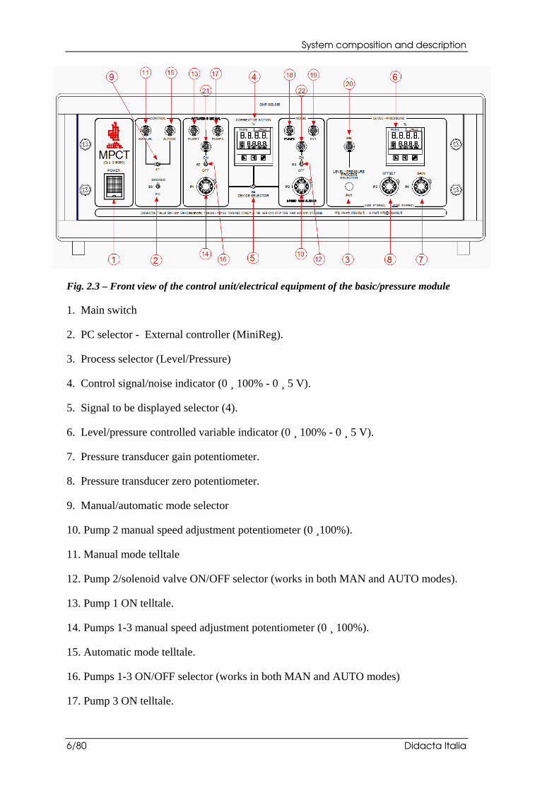
Fig. 2.3 – Front view of the control unit/electrical equipment of the basic/pressure module
1. Main switch
2. PC selector - External controller (MiniReg).
3. Process selector (Level/Pressure)
4. Control signal/noise indicator (0 ¸ 100% - 0 ¸ 5 V).
5. Signal to be displayed selector (4).
6. Level/pressure controlled variable indicator (0 ¸ 100% - 0 ¸ 5 V).
7. Pressure transducer gain potentiometer.
8. Pressure transducer zero potentiometer.
9. Manual/automatic mode selector
10. Pump 2 manual speed adjustment potentiometer (0 ¸100%).
11. Manual mode telltale
12. Pump 2/solenoid valve ON/OFF selector (works in both MAN and AUTO modes).
13. Pump 1 ON telltale.
14. Pumps 1-3 manual speed adjustment potentiometer (0 ¸ 100%).
15. Automatic mode telltale.
16. Pumps 1-3 ON/OFF selector (works in both MAN and AUTO modes)
17. Pump 3 ON telltale.
Chapter 2.
MPCT - User’s Manual 7/80
18. Pump 2 ON telltale.
19. EV1 solenoid valve ON telltale.
20. Level/pressure module ON telltale
21. Pumps 1-3 ON telltale.
22. Pump 2/ EV1 solenoid valve ON telltale.
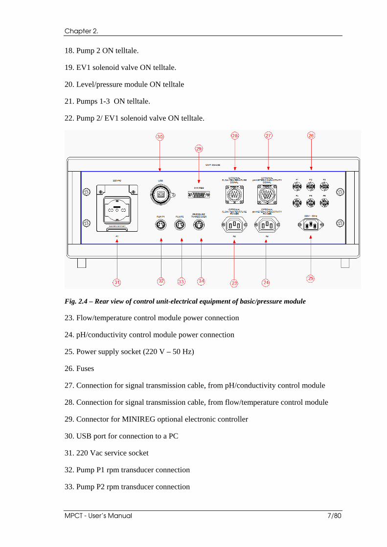
Fig. 2.4 – Rear view of control unit-electrical equipment of basic/pressure module
23. Flow/temperature control module power connection
24. pH/conductivity control module power connection
25. Power supply socket (220 V – 50 Hz)
26. Fuses
27. Connection for signal transmission cable, from pH/conductivity control module
28. Connection for signal transmission cable, from flow/temperature control module
29. Connector for MINIREG optional electronic controller
30. USB port for connection to a PC
31. 220 Vac service socket
32. Pump P1 rpm transducer connection
33. Pump P2 rpm transducer connection
System composition and description
8/80 Didacta Italia
34. Connection for pressure transducer
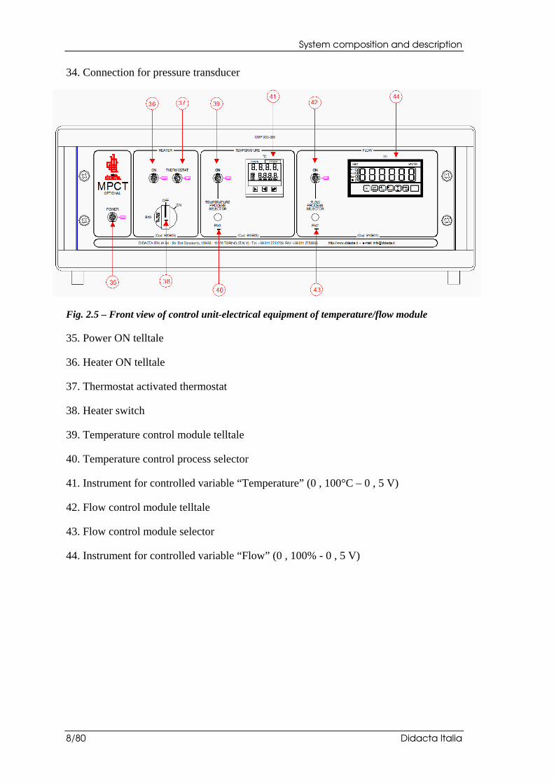
Fig. 2.5 – Front view of control unit-electrical equipment of temperature/flow module
35. Power ON telltale
36. Heater ON telltale
37. Thermostat activated thermostat
38. Heater switch
39. Temperature control module telltale
40. Temperature control process selector
41. Instrument for controlled variable “Temperature” (0 , 100°C – 0 , 5 V)
42. Flow control module telltale
43. Flow control module selector
44. Instrument for controlled variable “Flow” (0 , 100% - 0 , 5 V)
Chapter 2.
MPCT - User’s Manual 9/80
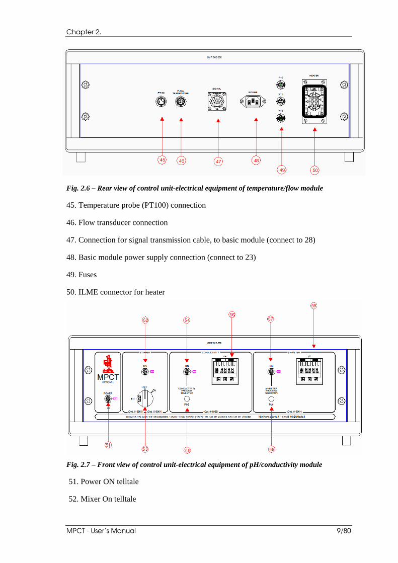
Fig. 2.6 – Rear view of control unit-electrical equipment of temperature/flow module
45. Temperature probe (PT100) connection
46. Flow transducer connection
47. Connection for signal transmission cable, to basic module (connect to 28)
48. Basic module power supply connection (connect to 23)
49. Fuses
50. ILME connector for heater
Fig. 2.7 – Front view of control unit-electrical equipment of pH/conductivity module
51. Power ON telltale
52. Mixer On telltale
System composition and description
10/80 Didacta Italia
53. Mixer switch
54. Conductivity control module telltale
55. Conductivity control process selector
56. Controlled variable indicator instrument for “Conductivity” (0 to 2000 nS/cm – 0 to 5 V)
57. pH control module telltale
58. pH control process selector
59. Controlled variable indicator instrument for “pH” (0 to 14 – 0 to 5 V)
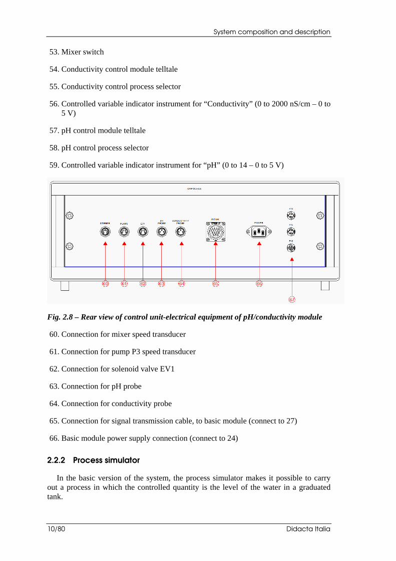
Fig. 2.8 – Rear view of control unit-electrical equipment of pH/conductivity module
60. Connection for mixer speed transducer
61. Connection for pump P3 speed transducer
62. Connection for solenoid valve EV1
63. Connection for pH probe
64. Connection for conductivity probe
65. Connection for signal transmission cable, to basic module (connect to 27)
66. Basic module power supply connection (connect to 24)
2.2.2 Process simulator
In the basic version of the system, the process simulator makes it possible to carry out a process in which the controlled quantity is the level of the water in a graduated tank.
Chapter 2.
MPCT - User’s Manual 11/80
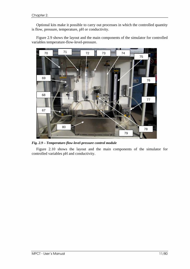
Optional kits make it possible to carry out processes in which the controlled quantity is flow, pressure, temperature, pH or conductivity.
Figure 2.9 shows the layout and the main components of the simulator for controlled variables temperature-flow-level-pressure.
Fig. 2.9 – Temperature-flow-level-pressure control module
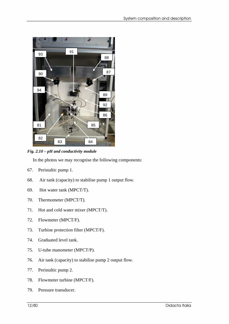
Figure 2.10 shows the layout and the main components of the simulator for controlled variables pH and conductivity.
67
68
69
70 71 72 73 7475
76
77
78 79
80
System composition and description
12/80 Didacta Italia
Fig. 2.10 – pH and conductivity module
In the photos we may recognise the following components:
67. Peristaltic pump 1.
68. Air tank (capacity) to stabilise pump 1 output flow.
69. Hot water tank (MPCT/T).
70. Thermometer (MPCT/T).
71. Hot and cold water mixer (MPCT/T).
72. Flowmeter (MPCT/F).
73. Turbine protection filter (MPCT/F).
74. Graduated level tank.
75. U-tube manometer (MPCT/P).
76. Air tank (capacity) to stabilise pump 2 output flow.
77. Peristaltic pump 2.
78. Flowmeter turbine (MPCT/F).
79. Pressure transducer.
82
81
83 84
85
86
87
88
89
90
91
92
93
94
Chapter 2.
MPCT - User’s Manual 13/80
80. Cold water tank.
81. Corrective substance tank
82. Corrective agent for pump P3
83. Process tank discharge outlet
84. Process tank
85. pH / conductivity probe
86. Noise: solenoid valve/process tank connection
87. Valve for manual adjustment of noise
88. Noise tank
89. Noise: tank/solenoid valve connection
90. Valve for manual adjustment of process
91. Solenoid valve
92. Feed tank/process connection
93. Process feed tank
94. Mixer
2.2.2.1 Temperature, level, pressure and flow control simulator
All four processes are simulated by means of peristaltic pumps 67 and 77, which are controlled by control signal, x, and noise signal, n, respectively.
During automatic control by either the PC or the MiniReg controller, pump 67 is controlled by control signal x and varies the flow so as to enable the controlled quantity to reach the Set-Point.
Pump 77 is controlled by the noise signal, n, and produces an independent flow that tends to disturb the process.
Both pumps have a maximum capacity of ca 7 l/h, and are controlled directly by a permanent magnet dc motor. Their action is controlled by the Personal Computer, or it may be controlled manually by means of the potentiometers fitted to the front panel of the electric module.
In all cases, these pumps affect the flow. To obtain the effect on the controlled quantity the system uses the following elements:
• graduated tank 74 for level;
System composition and description
14/80 Didacta Italia
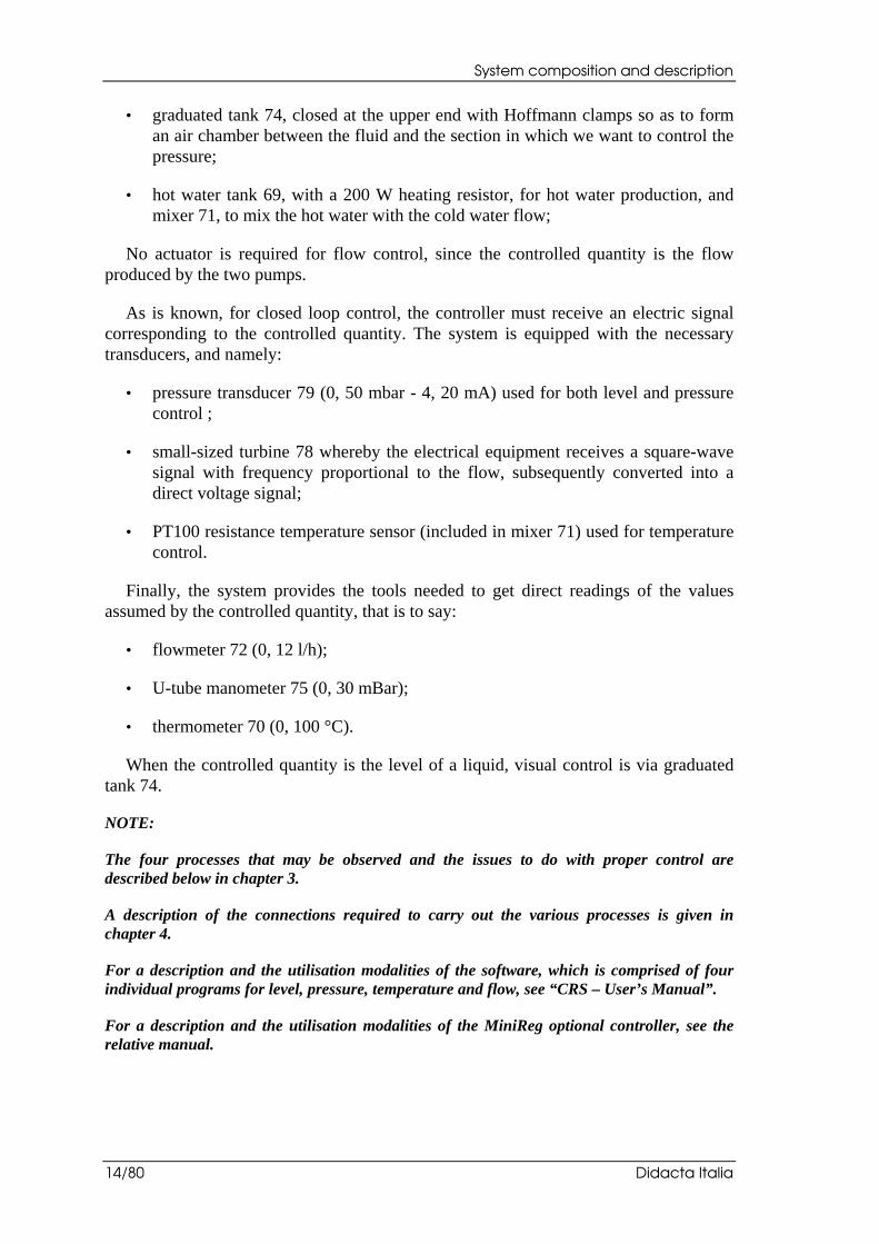
• graduated tank 74, closed at the upper end with Hoffmann clamps so as to form an air chamber between the fluid and the section in which we want to control the pressure;
• hot water tank 69, with a 200 W heating resistor, for hot water production, and mixer 71, to mix the hot water with the cold water flow;
No actuator is required for flow control, since the controlled quantity is the flow produced by the two pumps.
As is known, for closed loop control, the controller must receive an electric signal corresponding to the controlled quantity. The system is equipped with the necessary transducers, and namely:
• pressure transducer 79 (0, 50 mbar - 4, 20 mA) used for both level and pressure control ;
• small-sized turbine 78 whereby the electrical equipment receives a square-wave signal with frequency proportional to the flow, subsequently converted into a direct voltage signal;
• PT100 resistance temperature sensor (included in mixer 71) used for temperature control.
Finally, the system provides the tools needed to get direct readings of the values assumed by the controlled quantity, that is to say:
• flowmeter 72 (0, 12 l/h);
• U-tube manometer 75 (0, 30 mBar);
• thermometer 70 (0, 100 °C).
When the controlled quantity is the level of a liquid, visual control is via graduated tank 74.
NOTE:
The four processes that may be observed and the issues to do with proper control are described below in chapter 3.
A description of the connections required to carry out the various processes is given in chapter 4.
For a description and the utilisation modalities of the software, which is comprised of four individual programs for level, pressure, temperature and flow, see “CRS – User’s Manual”.
For a description and the utilisation modalities of the MiniReg optional controller, see the relative manual.
Chapter 2.
MPCT - User’s Manual 15/80
2.2.2.2 pH and conductivity control simulator
Tank 93 feeds process tank 84 continuously. The solution contained in it has a known pH, e.g., pH = 3. We want to change the pH of the solution to make it correspond to the set-point, which we assume to be 8. To this end, we start feeding the process tank with a basic substance (7<pH< 14) until we get a solution with a pH corresponding to the set-point, pH = 8. Pump P3 is responsible for the integrative action x. We can simulate an antagonist noise, n: to this end, we open a solenoid valve whereby an acid substance (0<pH<7) is released into the process tank from tank 88. The control action is through the PID system. For the control modalities of the pumps and the solenoid valve, see paragraph 2.2.2.3 below.
NOTE: For proper unit operation, set solenoid valve opening value to 0 % or 100%. (Valve fully closed or fully open).
The same module may be used for the control of the pH and the conductivity of the solution contained in process tank 84. The operating principle is the same in both processes. The only provision to be kept in mind when changing from one process to the other is to wash accurately the tanks and to change the probe, selecting the appropriate one and submerging it in the process tank. Washing the tanks and the probes is also required when, in using the module to control the pH of a solution, we go from a substance with basic pH to be acidified to a substance with acid pH to be basified. To ensure that they are emptied out completely, the tanks are fitted with discharge valves to be connected to the respective collection tanks. The tanks are also fitted with appropriate covers to facilitate the filling process.
NOTE: During pH control process, four different situations, which any other condition may be referred to, may occur:
1. set-point = 8 (BASIC); pH of initial solution = 5 : a BASIC substance must be added to increase the pH value of the controlled solution.
2. set-point = 8 (BASIC); pH of initial solution = 9 : an ACID substance must be added to reduce the pH value of the controlled solution.
3. set-point = 6 (ACID); pH of initial solution = 5 : a BASIC substance must be added to increase the pH value of the controlled solution.
4. set-point = 6 (ACID); pH of initial solution = 9 : an ACID substance must be added to reduce the pH value of the controlled solution.
2.2.2.3 Control unit and parameters viewing
Turn on the control unit by means of main switch 1: the selector lights up and the digital display units show the values of the associated quantities.
Selector 2 lets you decide whether you want the process to be controlled by means of the MINIREG external controller and the control unit or directly from the PC. If we set Selector 2 to “MINIREG”, selector 9 must be set to “MAN”: in this manner, the process is controlled manually through the MINIREG and telltale 11 lights up. At this point, we select the process control module that we want to use and activate it by means of switches 3, 40, 43, 55, 58, respectively. Now we start pumps P1 and P2 or pump P3 and
System composition and description
16/80 Didacta Italia
activate the EV1 solenoid valve by means of switches 16 or 12, depending on which process control we want to observe. If we are working in manual mode, pump speed is adjusted by means of potentiometers 10 and 14. The PC may no longer be used as a process control tool and is only used to view and save the test data. Conversely, if we set Selector 2 to “PC”, we must then set selector 9 to “AUTOM”: in this manner, the process is controlled through the PC. The parameters governing the system are set by means of the soft keys that appear in the various windows.
Display 4 makes it possible to view the value of the corrective action or the noise as a percentage of the corresponding maximum value. In the case of pumps P1, P2 and P3 we see the pump’s rotation speed as a percentage of the maximum value, i.e., since these are volumetric pumps, as a percentage of the maximum liquid flow that each pump is able to deliver to the system. In the case of the solenoid valve we see its opening as a percentage of corresponding maximum value.
NOTE: For proper unit operation, set solenoid valve opening value to 0 % or 100%. (Valve fully closed or fully open).
Selector 5 lets you decide which of the 4 parameters (speed P1, speed P2, speed P3, and solenoid valve opening) will be viewed on display 4. For example, if pumps P1 and P2 are running (pressure, level, temperature and flow control modules), then, on display 4, we shall read in alternation the speed of P1 /P2 % as a percentage of their max. rotation speed.
Display 6 proves useful when we work with the pressure module as well as with the level control module (even in level control, a pressure is measured, pressure being directly proportional to level). This display shows the level/pressure value as a percentage of the maximum value. The instrument must be calibrated as follows: with tank 41 full, adjust “GAIN” with potentiometer 7 so that the value shown on the display is “100”. Then, empty out the tank and adjust “OFFSET” with potentiometer 8 so that the value shown on the display is “0”. These two operations may have to be performed several times to complete the calibration process and have the two required values (“0” and “100”) appear on the display with the tank empty and full, respectively.
The control units are also equipped with a display to view the various processes: flow 44, temperature 41, pH 59, and conductivity 56. Additional elements include: mixer switch 53 to homogenize the solution whose pH we want to control (the switch has a telltale, 52, that lights up to indicate that the mixer is powered), and a heater, 38, for the temperature control module. The temperature control module also requires a safety thermostat, with telltale 36, that steps in when a temperature of 70°C is reached.
Chapter 3.
MPCT - User’s Manual 17/80
3. Description of the control processes and
techniques
3.1 Level control
3.1.1 Process description
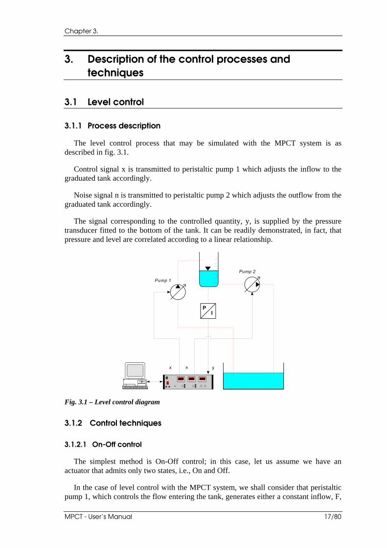
The level control process that may be simulated with the MPCT system is as described in fig. 3.1.
Control signal x is transmitted to peristaltic pump 1 which adjusts the inflow to the graduated tank accordingly.
Noise signal n is transmitted to peristaltic pump 2 which adjusts the outflow from the graduated tank accordingly.
The signal corresponding to the controlled quantity, y, is supplied by the pressure transducer fitted to the bottom of the tank. It can be readily demonstrated, in fact, that pressure and level are correlated according to a linear relationship.
Fig. 3.1 – Level control diagram
3.1.2 Control techniques
3.1.2.1 On-Off control
The simplest method is On-Off control; in this case, let us assume we have an actuator that admits only two states, i.e., On and Off.
In the case of level control with the MPCT system, we shall consider that peristaltic pump 1, which controls the flow entering the tank, generates either a constant inflow, F,
Description of the control processes and techniques
18/80 Didacta Italia
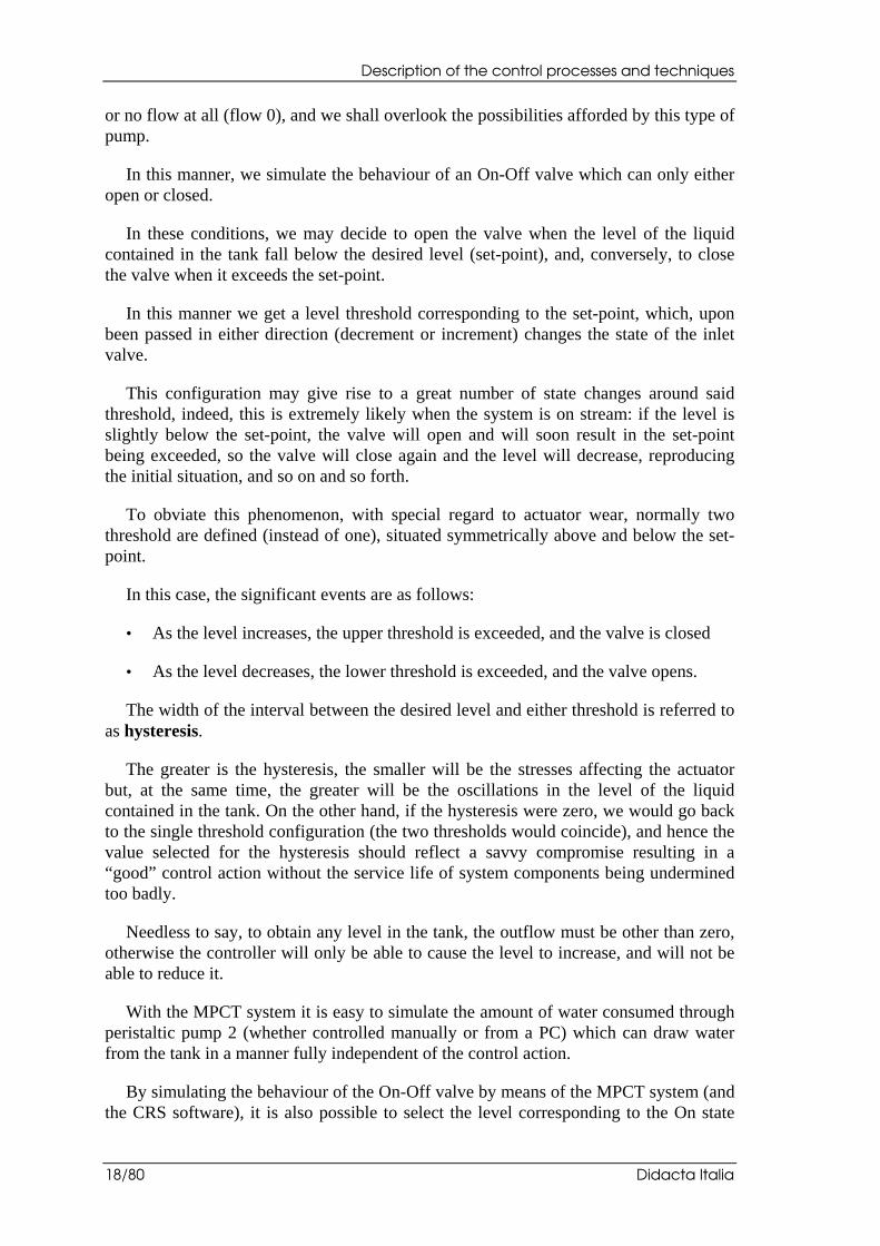
or no flow at all (flow 0), and we shall overlook the possibilities afforded by this type of pump.
In this manner, we simulate the behaviour of an On-Off valve which can only either open or closed.
In these conditions, we may decide to open the valve when the level of the liquid contained in the tank fall below the desired level (set-point), and, conversely, to close the valve when it exceeds the set-point.
In this manner we get a level threshold corresponding to the set-point, which, upon been passed in either direction (decrement or increment) changes the state of the inlet valve.
This configuration may give rise to a great number of state changes around said threshold, indeed, this is extremely likely when the system is on stream: if the level is slightly below the set-point, the valve will open and will soon result in the set-point being exceeded, so the valve will close again and the level will decrease, reproducing the initial situation, and so on and so forth.
To obviate this phenomenon, with special regard to actuator wear, normally two threshold are defined (instead of one), situated symmetrically above and below the set-point.
In this case, the significant events are as follows:
• As the level increases, the upper threshold is exceeded, and the valve is closed
• As the level decreases, the lower threshold is exceeded, and the valve opens.
The width of the interval between the desired level and either threshold is referred to as hysteresis.
The greater is the hysteresis, the smaller will be the stresses affecting the actuator but, at the same time, the greater will be the oscillations in the level of the liquid contained in the tank. On the other hand, if the hysteresis were zero, we would go back to the single threshold configuration (the two thresholds would coincide), and hence the value selected for the hysteresis should reflect a savvy compromise resulting in a “good” control action without the service life of system components being undermined too badly.
Needless to say, to obtain any level in the tank, the outflow must be other than zero, otherwise the controller will only be able to cause the level to increase, and will not be able to reduce it.
With the MPCT system it is easy to simulate the amount of water consumed through peristaltic pump 2 (whether controlled manually or from a PC) which can draw water from the tank in a manner fully independent of the control action.
By simulating the behaviour of the On-Off valve by means of the MPCT system (and the CRS software), it is also possible to select the level corresponding to the On state
Chapter 3.
MPCT - User’s Manual 19/80
(not necessarily corresponding to 100 % of maximum opening) and the valve switch-over time from one state to the other (normally, a motorised valve requires a certain time interval, other than zero).
3.1.2.2 PID control
General
In the previous case we simulated a system equipped with an On-Off valve.
However, we may consider adopting a valve whose opening will vary continuously from 0 to a maximum value. A valve possessing such characteristics is referred to as Proportional, in that its degree of opening is proportional to the electric control signal.
Needless to say, in the MPCT system, the peristaltic pumps are able to simulate the behaviour of a proportional valve.
In a wide range of applications, the control system is obtained through the contribution of three components:
• proportional
• integral
• derivative
The control signal, determined on the basis of the error observed (i.e., the difference between the desired value (the set-point) for the controlled quantity and the value actually detected), is given by sum of three terms, of which the first is proportional to said error, the second is proportional to its integral over time, and the third is proportional to its derivative (which supplies the “trend” of the error).
In the following paragraphs, the various terms are discussed in greater detail.
Proportional components
As mentioned before, this component is proportional to the error, i.e., the difference between the set-point and the measured value.
Hence, it may be characterised by the value of the proportionality constant.
When the control signal reaches 100% of its possible value, in our case when pump 1 delivers maximum flow, the error reaches a “saturation level”.
Any error increment will not longer give rise to an increment in the control signal.
To impose a given saturation level means to establish an error interval within which the control signal will assume an intermediate value between 0% and 100%, and outside which the value of the control signal will be 0% and 100%, respectively.
The error variation band is referred to as Proportional Band (P-Band).
Description of the control processes and techniques
20/80 Didacta Italia
Given an error e, i.e., an error comprised between 0 and the P-Band, the percentage value of the control signal, x, is given by:
x = e 100
P Band
The error being the same, the greater is the P-Band, the smaller will be the controller output signal, x; i.e., the smaller will be the proportional gain of the controller.
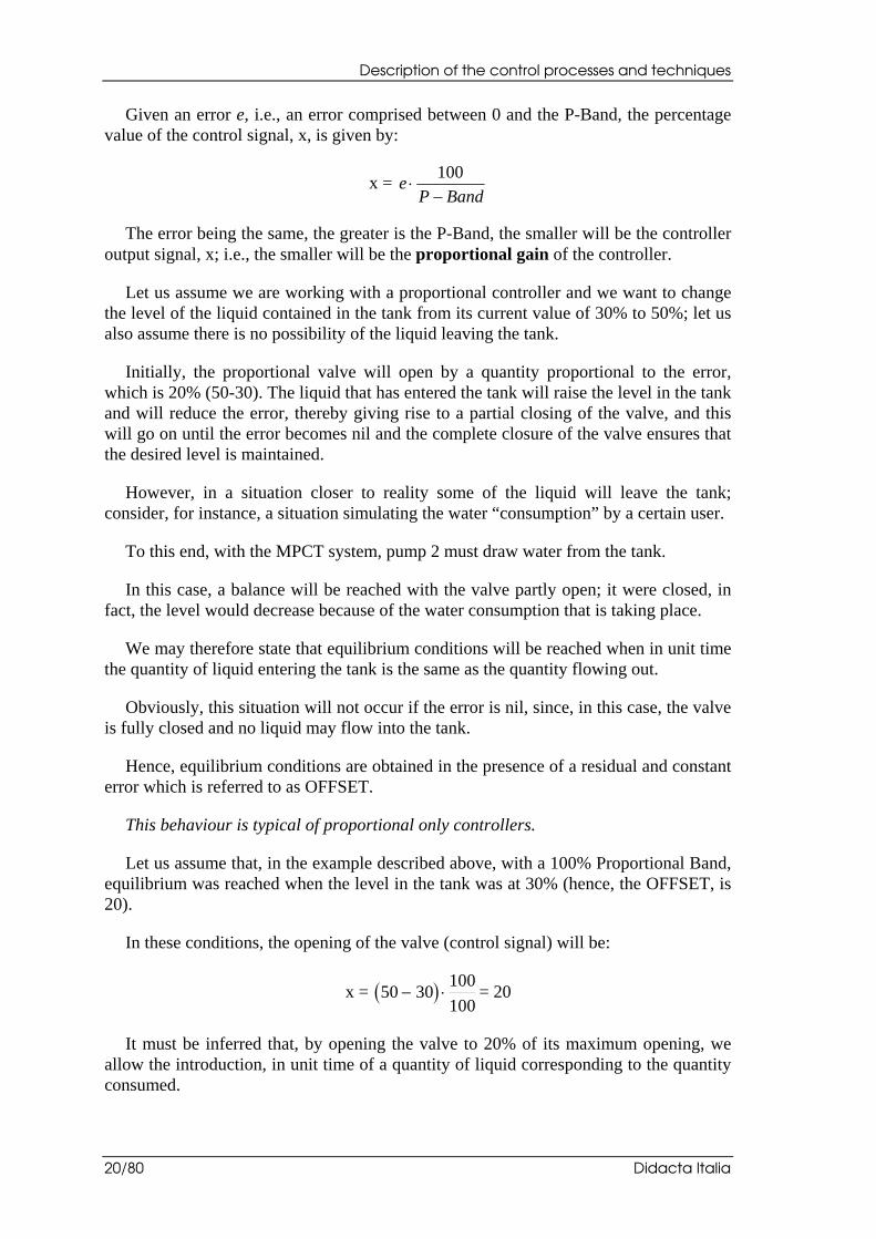
Let us assume we are working with a proportional controller and we want to change the level of the liquid contained in the tank from its current value of 30% to 50%; let us also assume there is no possibility of the liquid leaving the tank.
Initially, the proportional valve will open by a quantity proportional to the error, which is 20% (50-30). The liquid that has entered the tank will raise the level in the tank and will reduce the error, thereby giving rise to a partial closing of the valve, and this will go on until the error becomes nil and the complete closure of the valve ensures that the desired level is maintained.
However, in a situation closer to reality some of the liquid will leave the tank; consider, for instance, a situation simulating the water “consumption” by a certain user.
To this end, with the MPCT system, pump 2 must draw water from the tank.
In this case, a balance will be reached with the valve partly open; it were closed, in fact, the level would decrease because of the water consumption that is taking place.
We may therefore state that equilibrium conditions will be reached when in unit time the quantity of liquid entering the tank is the same as the quantity flowing out.
Obviously, this situation will not occur if the error is nil, since, in this case, the valve is fully closed and no liquid may flow into the tank.
Hence, equilibrium conditions are obtained in the presence of a residual and constant error which is referred to as OFFSET.
This behaviour is typical of proportional only controllers.
Let us assume that, in the example described above, with a 100% Proportional Band, equilibrium was reached when the level in the tank was at 30% (hence, the OFFSET, is 20).
In these conditions, the opening of the valve (control signal) will be:
x = 50 30100
100 = 20
It must be inferred that, by opening the valve to 20% of its maximum opening, we allow the introduction, in unit time of a quantity of liquid corresponding to the quantity consumed.
Chapter 3.
MPCT - User’s Manual 21/80
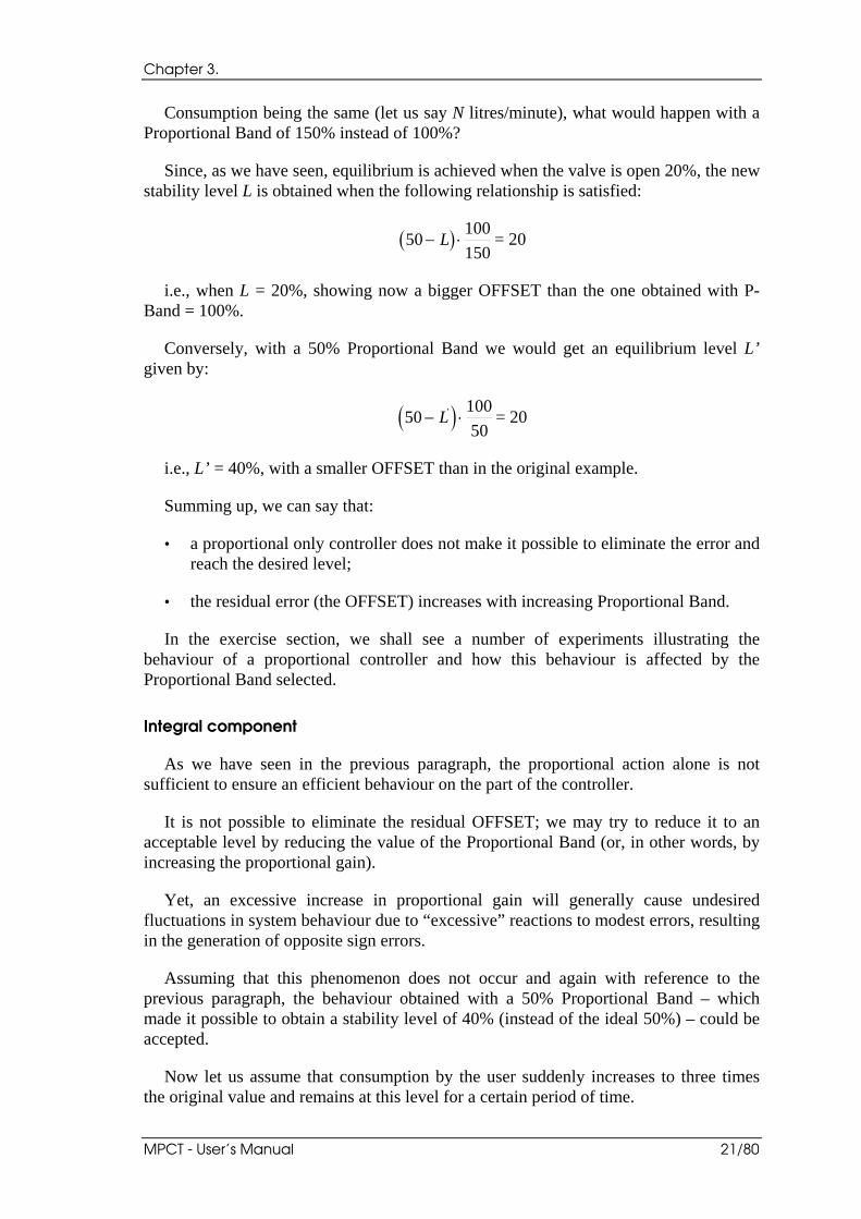
Consumption being the same (let us say N litres/minute), what would happen with a Proportional Band of 150% instead of 100%?
Since, as we have seen, equilibrium is achieved when the valve is open 20%, the new stability level L is obtained when the following relationship is satisfied:
50100
150 L = 20
i.e., when L = 20%, showing now a bigger OFFSET than the one obtained with P-Band = 100%.
Conversely, with a 50% Proportional Band we would get an equilibrium level L’ given by:
50100
50 L' = 20
i.e., L’ = 40%, with a smaller OFFSET than in the original example.
Summing up, we can say that:
• a proportional only controller does not make it possible to eliminate the error and reach the desired level;
• the residual error (the OFFSET) increases with increasing Proportional Band.
In the exercise section, we shall see a number of experiments illustrating the behaviour of a proportional controller and how this behaviour is affected by the Proportional Band selected.
Integral component
As we have seen in the previous paragraph, the proportional action alone is not sufficient to ensure an efficient behaviour on the part of the controller.
It is not possible to eliminate the residual OFFSET; we may try to reduce it to an acceptable level by reducing the value of the Proportional Band (or, in other words, by increasing the proportional gain).
Yet, an excessive increase in proportional gain will generally cause undesired fluctuations in system behaviour due to “excessive” reactions to modest errors, resulting in the generation of opposite sign errors.
Assuming that this phenomenon does not occur and again with reference to the previous paragraph, the behaviour obtained with a 50% Proportional Band – which made it possible to obtain a stability level of 40% (instead of the ideal 50%) – could be accepted.
Now let us assume that consumption by the user suddenly increases to three times the original value and remains at this level for a certain period of time.
Description of the control processes and techniques
22/80 Didacta Italia
This situation may correspond to a situation that occurs in actual practice in a water distribution system during some hourly bands.
In the stability conditions in which the phenomenon occurs, the valve is open 20% of its maximum opening value which enables it to “offset” exactly the original consumption.
But now this “compensation” is no longer sufficient and the level in the tank will inevitably decrease.
As the error increases, the valve opens to an increasing degree and a new equilibrium will be obtained as soon as the opening is sufficient to compensate for the new consumption rate.
Under the foregoing assumptions, this will happen when valve opening is 60% (three times the starting value); in these new conditions, however, the stability level of the tank, L”, will be given by the habitual formula:
50100
50 L" = 60
i.e., L” = 20%.
The only chance to establish a level closer to the starting level is to change the set-point in a clearly “arbitrary” manner, by increasing it, for instance, to 80%!
By adding an integral component to the proportional component, the problem can be remedied without any “unnatural” intervention by the system manager.
The behaviour described above, in fact, shows that the system is insensitive to “small” residual errors: this is the reason why, in this case, it is not possible to make appropriate corrections.
A proportional and integral controller (sometimes called delay compensator) evaluates the control quantity as the (algebraic) sum of the proportional component as described above and a term proportional to the integral of the error over time:
x (t) = K e t K e dp i
t
0
The integral component of the control action eliminates the residual error associated with proportional only control.
Let us assume we start from conditions of perfect stability, where the level of the liquid contained in the tank is 50%, i.e., corresponds to the desired set-point, and consumption is zero.
In these conditions the valve is fully closed there being no liquid outflow to be compensated for and the desired level has been reached.
Chapter 3.
MPCT - User’s Manual 23/80
If at a certain time, t = 0, a sudden increase in demand occurred, which (as we have seen in one of the previous examples) can be compensated for by a 20% delivery, the level would decrease initially and then would start increasing thanks to the action of the controller.
But this time, this action is not determined solely by the value assumed by the error over time, but also by its “history”: in other works, the fact that during the initial stage of the phenomenon, the error increased and then decreased at a later stage, entails a non nil integral component that contributes to the formation of the control signal and that remains such (non nil) even when the set-point has been reached.
It is therefore possible to eliminate the error altogether even when, as in this case, the new stability situation requires the addition of liquid to the tank: this is done thanks to the second of the terms specified above, i.e., the integral one, whereas the first, the proportional term, makes no contribution in this situation.
In general, a proportional-integral controller is widely used when one expects wide but slow variations in the controlled quantity, requiring decisive changes in the control signal. The case of level control therefore lends itself well to the use of this type of device.
Derivative component
The control action is often improved by supplementing the two – proportional and integral – components discussed above with a component that is proportional to the derivative of the error (as it varies over time).
x (t) = K e t K e d Kd
dte tp i
t
d 0
( )
The derivative component, whose action is associated with the “trend” of the error , has an anticipatory effect on the global action of the controller.
This component, in fact, determines a contribution based on the rate of change of the error: the higher the rate at which the error is increasing, for instance, the greater will be the contribution of the derivative component that, in this manner, carries out in advance an action that otherwise would have to be performed later on.
If the error remains constant, its derivative over time is nil and the contribution due to the presence of a derivative component is also nil.
If the error is not constant, but varies slowly, the situation is similar to the one described above and hence the contribution arising from the presence of a derivative component should be sought in all those situations in which variations are expected to take place rapidly and within small load limits.
As mentioned in the previous paragraph, level control is characterised by load variations that are quite slow (the process manifests a certain inertia due to the fact that the controlled quantity, i.e., level, increases with the integral of the control signal, which in actual fact acts on the flow).
Description of the control processes and techniques
24/80 Didacta Italia
Accordingly, the derivative of the error assumes small values and the action of a derivative component (proportional to said derivative) is of little significance.
Chapter 3.
MPCT - User’s Manual 25/80
3.2 Flow control
3.2.1 Process description
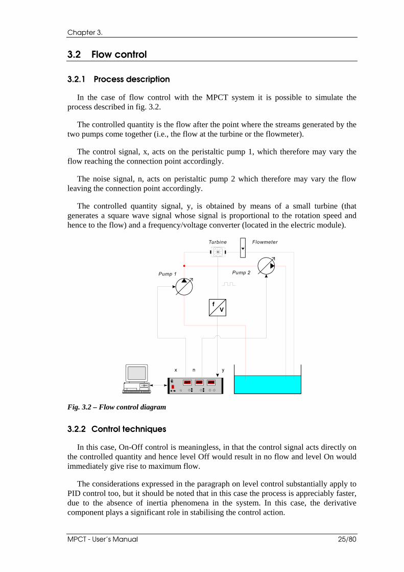
In the case of flow control with the MPCT system it is possible to simulate the process described in fig. 3.2.
The controlled quantity is the flow after the point where the streams generated by the two pumps come together (i.e., the flow at the turbine or the flowmeter).
The control signal, x, acts on the peristaltic pump 1, which therefore may vary the flow reaching the connection point accordingly.
The noise signal, n, acts on peristaltic pump 2 which therefore may vary the flow leaving the connection point accordingly.
The controlled quantity signal, y, is obtained by means of a small turbine (that generates a square wave signal whose signal is proportional to the rotation speed and hence to the flow) and a frequency/voltage converter (located in the electric module).
Fig. 3.2 – Flow control diagram
3.2.2 Control techniques
In this case, On-Off control is meaningless, in that the control signal acts directly on the controlled quantity and hence level Off would result in no flow and level On would immediately give rise to maximum flow.
The considerations expressed in the paragraph on level control substantially apply to PID control too, but it should be noted that in this case the process is appreciably faster, due to the absence of inertia phenomena in the system. In this case, the derivative component plays a significant role in stabilising the control action.
Description of the control processes and techniques
26/80 Didacta Italia
3.3 Pressure control
3.3.1 Process description
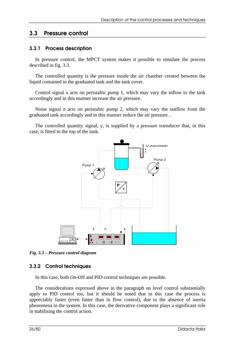
In pressure control, the MPCT system makes it possible to simulate the process described in fig. 3.3.
The controlled quantity is the pressure inside the air chamber created between the liquid contained in the graduated tank and the tank cover.
Control signal x acts on peristaltic pump 1, which may vary the inflow to the tank accordingly and in this manner increase the air pressure.
Noise signal n acts on peristaltic pump 2, which may vary the outflow from the graduated tank accordingly and in this manner reduce the air pressure. .
The controlled quantity signal, y, is supplied by a pressure transducer that, in this case, is fitted to the top of the tank.
Fig. 3.3 – Pressure control diagram
3.3.2 Control techniques
In this case, both On-Off and PID control techniques are possible.
The considerations expressed above in the paragraph on level control substantially apply to PID control too, but it should be noted that in this case the process is appreciably faster (even faster than in flow control), due to the absence of inertia phenomena in the system. In this case, the derivative component plays a significant role in stabilising the control action.
Chapter 3.
MPCT - User’s Manual 27/80
3.4 Temperature control
3.4.1 Process description
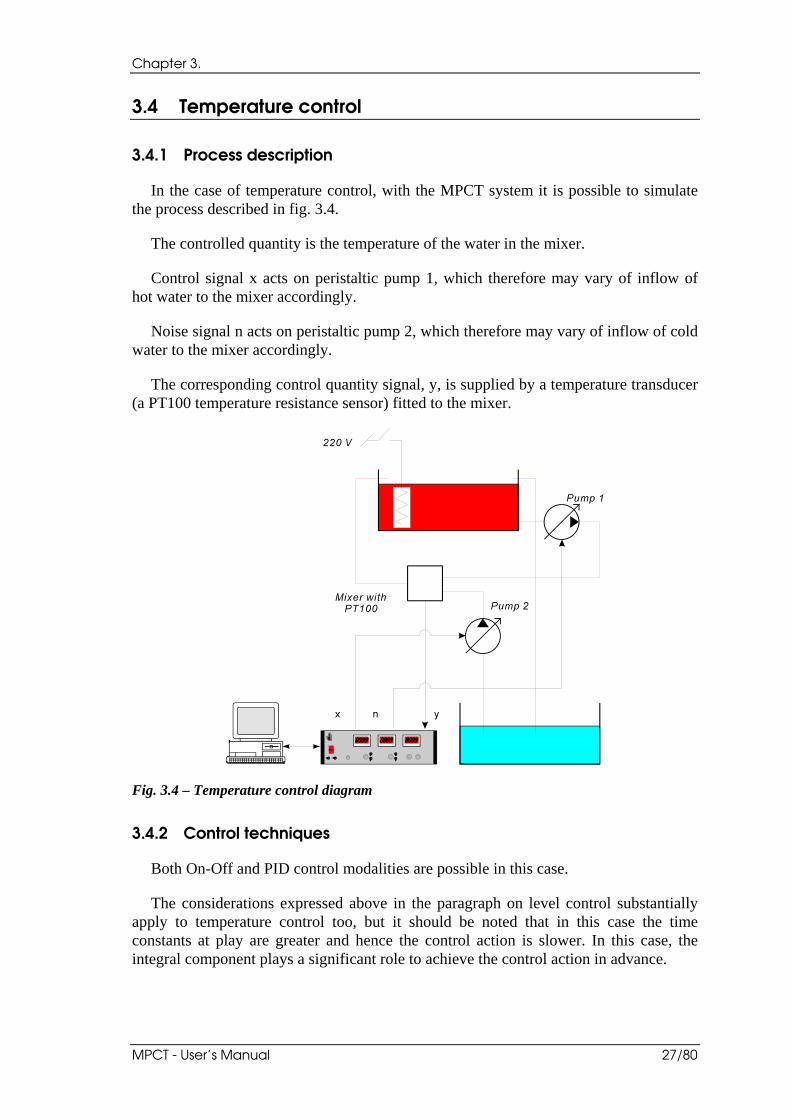
In the case of temperature control, with the MPCT system it is possible to simulate the process described in fig. 3.4.
The controlled quantity is the temperature of the water in the mixer.
Control signal x acts on peristaltic pump 1, which therefore may vary of inflow of hot water to the mixer accordingly.
Noise signal n acts on peristaltic pump 2, which therefore may vary of inflow of cold water to the mixer accordingly.
The corresponding control quantity signal, y, is supplied by a temperature transducer (a PT100 temperature resistance sensor) fitted to the mixer.
Fig. 3.4 – Temperature control diagram
3.4.2 Control techniques
Both On-Off and PID control modalities are possible in this case.
The considerations expressed above in the paragraph on level control substantially apply to temperature control too, but it should be noted that in this case the time constants at play are greater and hence the control action is slower. In this case, the integral component plays a significant role to achieve the control action in advance.
Description of the control processes and techniques
28/80 Didacta Italia
3.5 pH and conductivity control
3.5.1 Process description
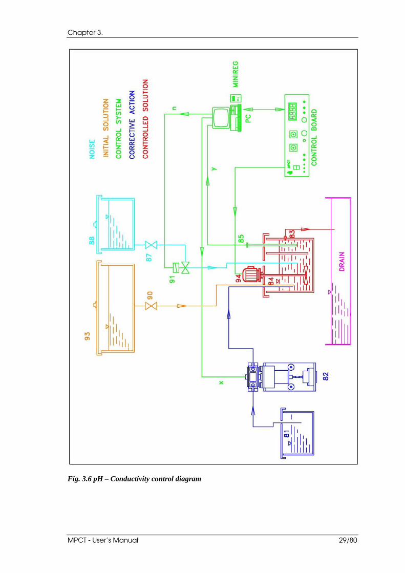
In the case of pH and conductivity control, with the MPCT system it is possible to simulate the process described in fig. 3.6.
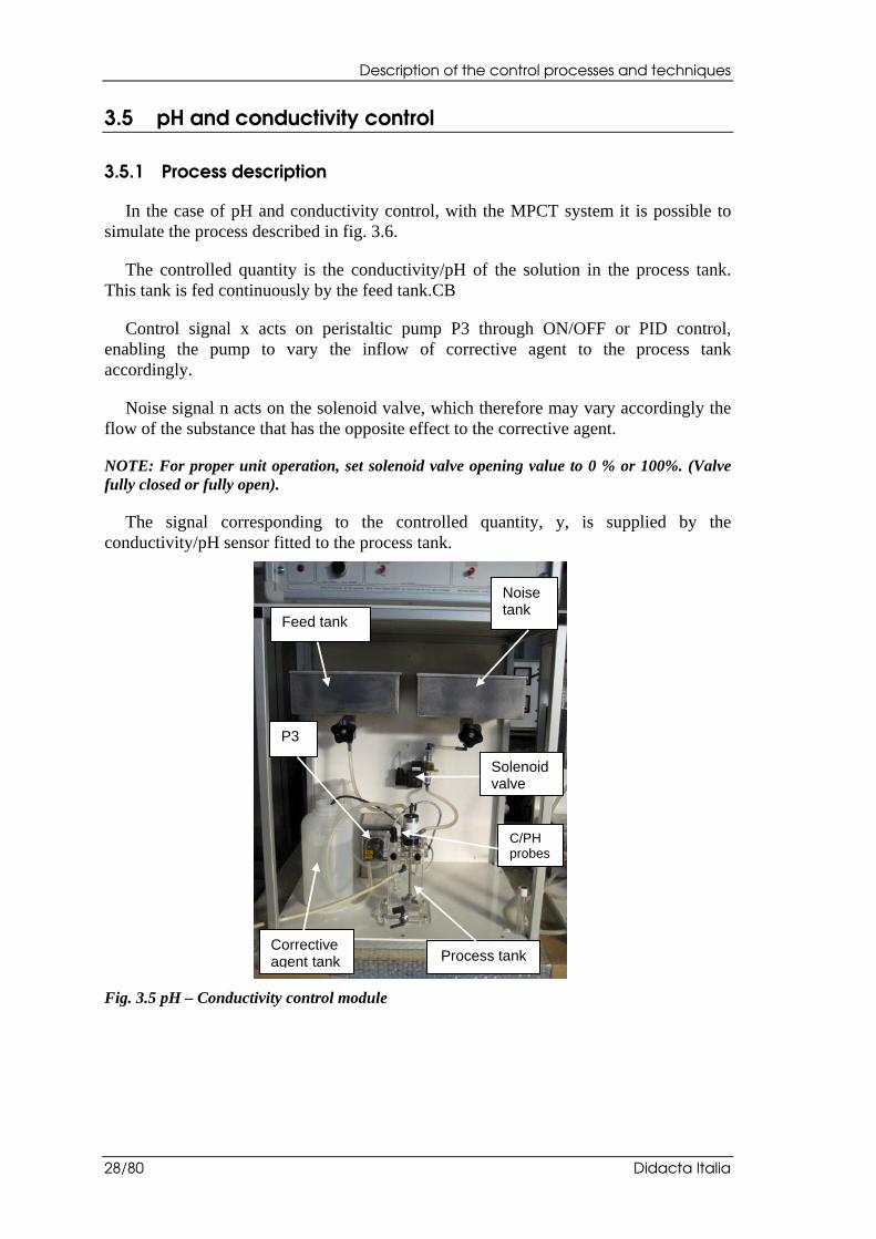
The controlled quantity is the conductivity/pH of the solution in the process tank. This tank is fed continuously by the feed tank.CB
Control signal x acts on peristaltic pump P3 through ON/OFF or PID control, enabling the pump to vary the inflow of corrective agent to the process tank accordingly.
Noise signal n acts on the solenoid valve, which therefore may vary accordingly the flow of the substance that has the opposite effect to the corrective agent.
NOTE: For proper unit operation, set solenoid valve opening value to 0 % or 100%. (Valve fully closed or fully open).
The signal corresponding to the controlled quantity, y, is supplied by the conductivity/pH sensor fitted to the process tank.
Fig. 3.5 pH – Conductivity control module
Feed tank
Corrective agent tank Process tank
P3
Noise tank
C/PH probes
Solenoid valve
Chapter 3.
MPCT - User’s Manual 29/80
Fig. 3.6 pH – Conductivity control diagram
Description of the control processes and techniques
30/80 Didacta Italia
3.5.2 Control techniques
Both On-Off and PID control modalities are possible in this case.
The considerations expressed above in the paragraph on level control substantially apply to pH and conductivity control too, but it should be noted that in this case the time constants at play are greater and hence the control action is slower. In this case, the integral component plays a significant role to achieve the control action in advance.
Chapter 4.
MPCT - User’s Manual 31/80
4. Installation and preliminary operations
4.1 Level control
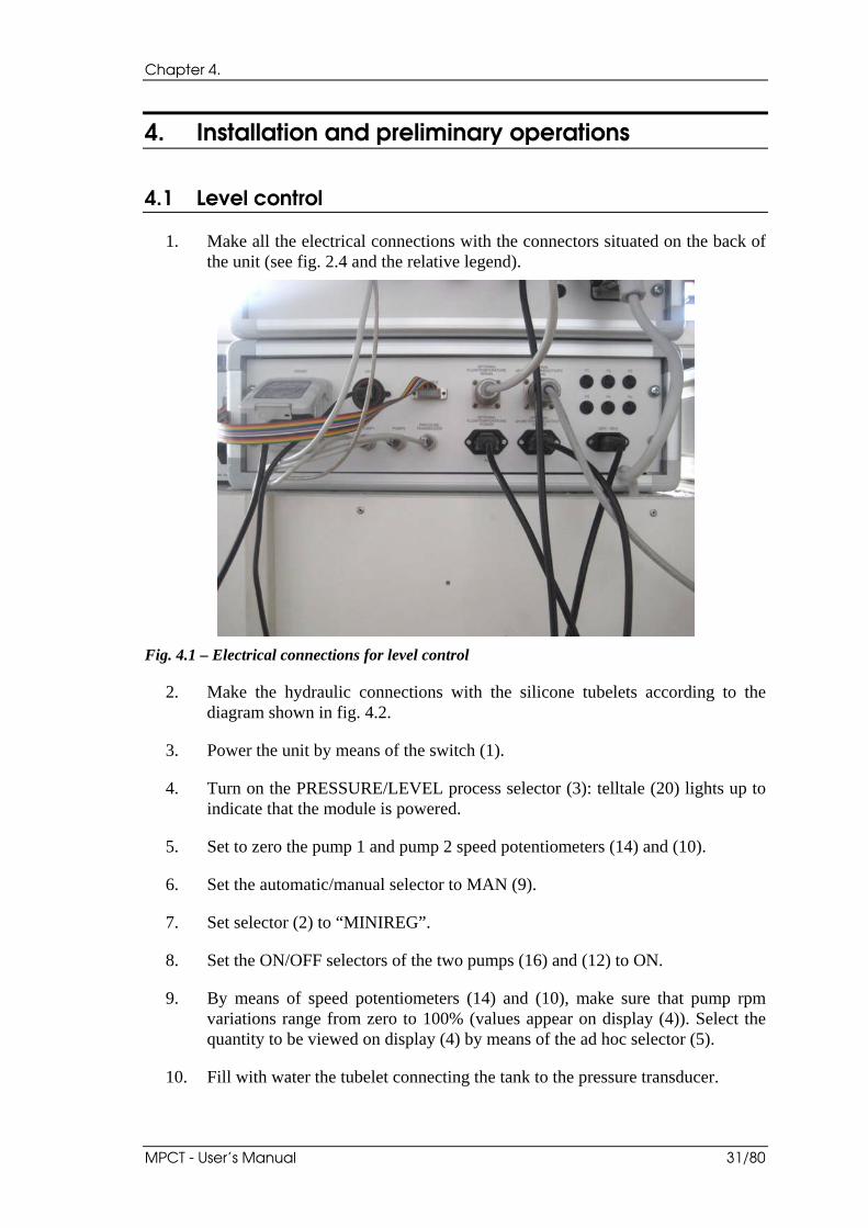
1. Make all the electrical connections with the connectors situated on the back of the unit (see fig. 2.4 and the relative legend).
Fig. 4.1 – Electrical connections for level control
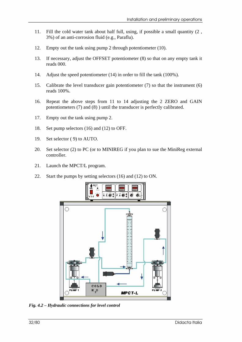
2. Make the hydraulic connections with the silicone tubelets according to the diagram shown in fig. 4.2.
3. Power the unit by means of the switch (1).
4. Turn on the PRESSURE/LEVEL process selector (3): telltale (20) lights up to indicate that the module is powered.
5. Set to zero the pump 1 and pump 2 speed potentiometers (14) and (10).
6. Set the automatic/manual selector to MAN (9).
7. Set selector (2) to “MINIREG”.
8. Set the ON/OFF selectors of the two pumps (16) and (12) to ON.
9. By means of speed potentiometers (14) and (10), make sure that pump rpm variations range from zero to 100% (values appear on display (4)). Select the quantity to be viewed on display (4) by means of the ad hoc selector (5).
10. Fill with water the tubelet connecting the tank to the pressure transducer.
Installation and preliminary operations
32/80 Didacta Italia
11. Fill the cold water tank about half full, using, if possible a small quantity (2 , 3%) of an anti-corrosion fluid (e.g., Paraflu).
12. Empty out the tank using pump 2 through potentiometer (10).
13. If necessary, adjust the OFFSET potentiometer (8) so that on any empty tank it reads 000.
14. Adjust the speed potentiometer (14) in order to fill the tank (100%).
15. Calibrate the level transducer gain potentiometer (7) so that the instrument (6) reads 100%.
16. Repeat the above steps from 11 to 14 adjusting the 2 ZERO and GAIN potentiometers (7) and (8) ) until the transducer is perfectly calibrated.
17. Empty out the tank using pump 2.
18. Set pump selectors (16) and (12) to OFF.
19. Set selector ( 9) to AUTO.
20. Set selector (2) to PC (or to MINIREG if you plan to sue the MiniReg external controller.
21. Launch the MPCT/L program.
22. Start the pumps by setting selectors (16) and (12) to ON.
Fig. 4.2 – Hydraulic connections for level control
Chapter 4.
MPCT - User’s Manual 33/80
4.2 Flow control
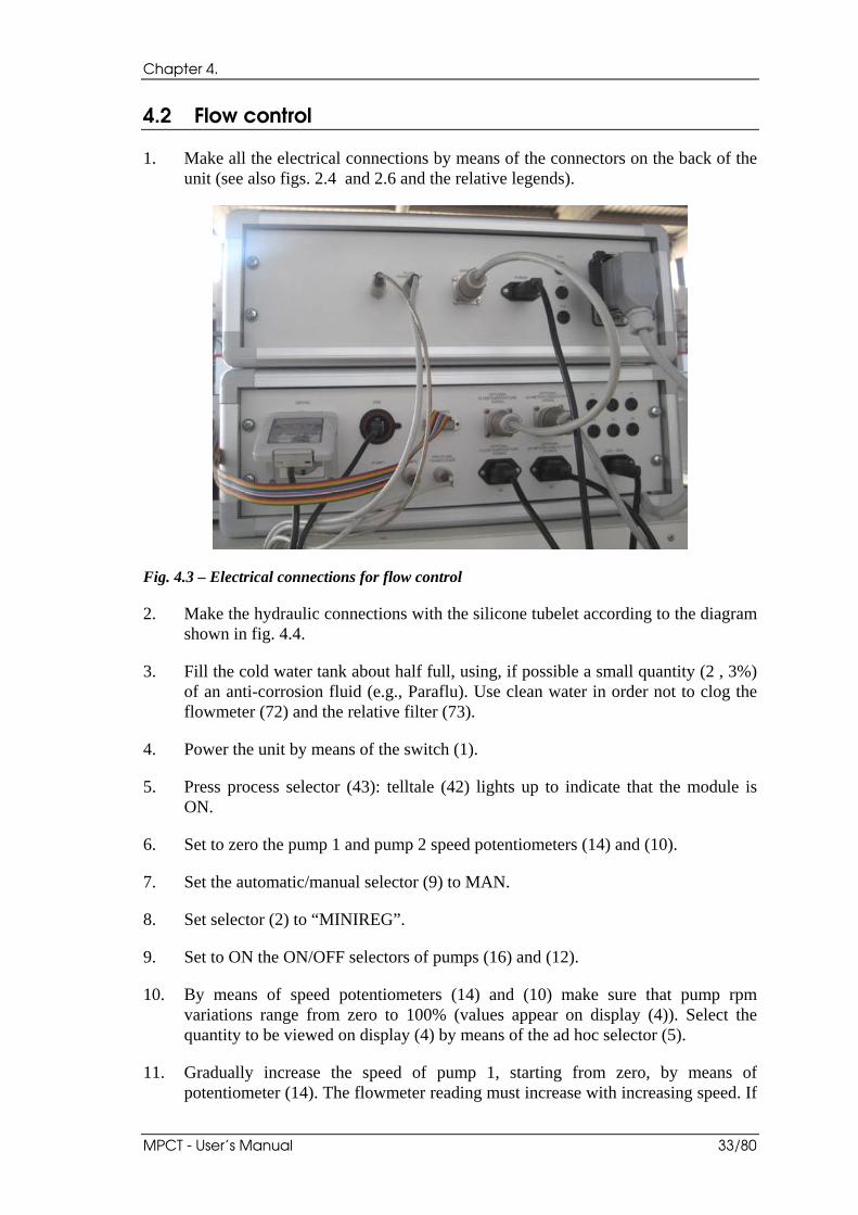
1. Make all the electrical connections by means of the connectors on the back of the unit (see also figs. 2.4 and 2.6 and the relative legends).
Fig. 4.3 – Electrical connections for flow control
2. Make the hydraulic connections with the silicone tubelet according to the diagram shown in fig. 4.4.
3. Fill the cold water tank about half full, using, if possible a small quantity (2 , 3%) of an anti-corrosion fluid (e.g., Paraflu). Use clean water in order not to clog the flowmeter (72) and the relative filter (73).
4. Power the unit by means of the switch (1).
5. Press process selector (43): telltale (42) lights up to indicate that the module is ON.
6. Set to zero the pump 1 and pump 2 speed potentiometers (14) and (10).
7. Set the automatic/manual selector (9) to MAN.
8. Set selector (2) to “MINIREG”.
9. Set to ON the ON/OFF selectors of pumps (16) and (12).
10. By means of speed potentiometers (14) and (10) make sure that pump rpm variations range from zero to 100% (values appear on display (4)). Select the quantity to be viewed on display (4) by means of the ad hoc selector (5).
11. Gradually increase the speed of pump 1, starting from zero, by means of potentiometer (14). The flowmeter reading must increase with increasing speed. If
Installation and preliminary operations
34/80 Didacta Italia
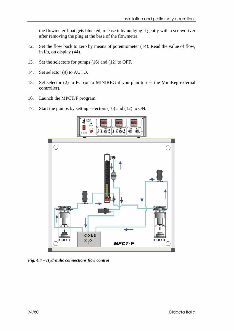
the flowmeter float gets blocked, release it by nudging it gently with a screwdriver after removing the plug at the base of the flowmeter.
12. Set the flow back to zero by means of potentiometer (14). Read the value of flow, in l/h, on display (44).
13. Set the selectors for pumps (16) and (12) to OFF.
14. Set selector (9) to AUTO.
15. Set selector (2) to PC (or to MINIREG if you plan to use the MiniReg external controller).
16. Launch the MPCT/F program.
17. Start the pumps by setting selectors (16) and (12) to ON.
Fig. 4.4 – Hydraulic connections flow control
Chapter 4.
MPCT - User’s Manual 35/80
4.3 Pressure control
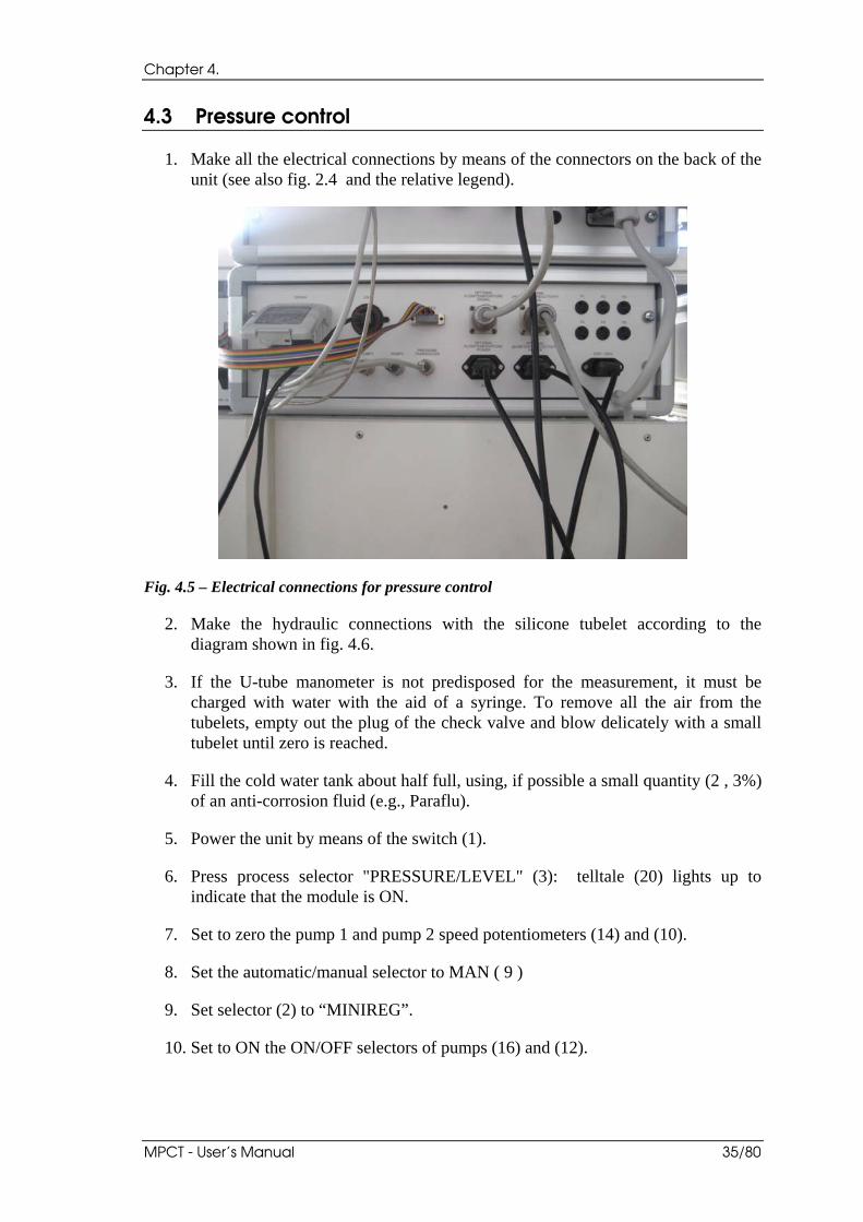
1. Make all the electrical connections by means of the connectors on the back of the unit (see also fig. 2.4 and the relative legend).
Fig. 4.5 – Electrical connections for pressure control
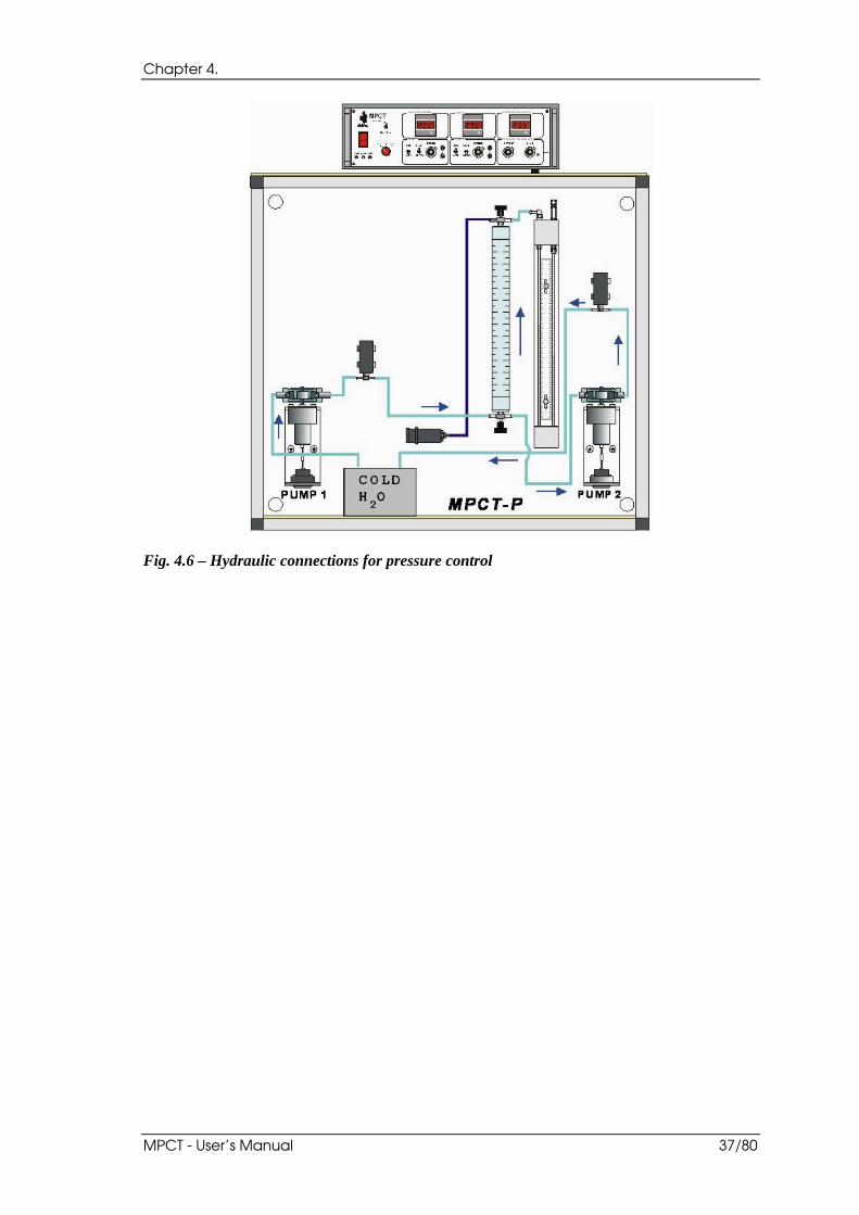
2. Make the hydraulic connections with the silicone tubelet according to the diagram shown in fig. 4.6.
3. If the U-tube manometer is not predisposed for the measurement, it must be charged with water with the aid of a syringe. To remove all the air from the tubelets, empty out the plug of the check valve and blow delicately with a small tubelet until zero is reached.
4. Fill the cold water tank about half full, using, if possible a small quantity (2 , 3%) of an anti-corrosion fluid (e.g., Paraflu).
5. Power the unit by means of the switch (1).
6. Press process selector "PRESSURE/LEVEL" (3): telltale (20) lights up to indicate that the module is ON.
7. Set to zero the pump 1 and pump 2 speed potentiometers (14) and (10).
8. Set the automatic/manual selector to MAN ( 9 )
9. Set selector (2) to “MINIREG”.
10. Set to ON the ON/OFF selectors of pumps (16) and (12).
Installation and preliminary operations
36/80 Didacta Italia
11. By means of speed potentiometers (14) and (10), make sure that pump rpm variations range from zero to 100% (values appear on display (4)). Select the quantity to be viewed on display (4) by means of the ad hoc selector (5).
9. In manual mode set the pressure back to zero by means of pump P1 and potentiometer (14).
10. Make sure that for zero pressure the transducer sends a zero V signal; if this is not the case, adjust by means of the OFFSET potentiometer (8).
11. Working manually on pump 1, starting from zero rpm increase speed until a pressure of 300 mm water column (max. pressure) is reached. Keeping mind that exceedingly high pressures may damage the transducer: make sure pressure never exceeds 200 mBar.
12. Make sure that instrument (6) reads 100%. If necessary, adjust the gain potentiometer (7).
13. Repeat the above steps from 11 to 14 using the 2 OFFSET and GAIN potentiometers (7) and (8) until the transducer is perfectly calibrated.
14. Set the pressure back to zero by means of potentiometer (14).
15. Set the selectors for pumps (16) and (12) to OFF.
16. Set selector (9) to AUTOM.
17. Set selector (2) to PC (or to MINIREG if you plan to use the MiniReg external controller).
18. Launch the MPCT/P program.
19. Start the pumps by setting selectors (16) and (12) to ON
Chapter 4.
MPCT - User’s Manual 37/80
Fig. 4.6 – Hydraulic connections for pressure control
Installation and preliminary operations
38/80 Didacta Italia
4.4 Temperature control
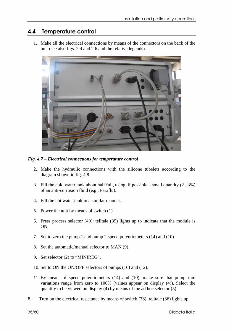
1. Make all the electrical connections by means of the connectors on the back of the unit (see also figs. 2.4 and 2.6 and the relative legends).
Fig. 4.7 – Electrical connections for temperature control
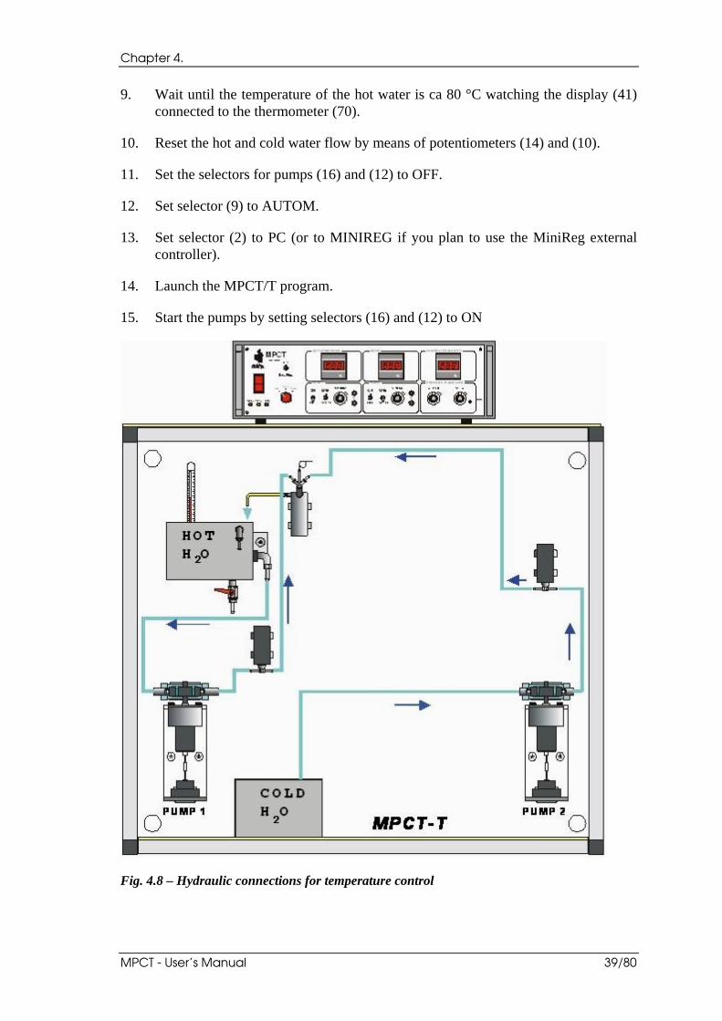
2. Make the hydraulic connections with the silicone tubelets according to the diagram shown in fig. 4.8.
3. Fill the cold water tank about half full, using, if possible a small quantity (2 , 3%) of an anti-corrosion fluid (e.g., Paraflu).
4. Fill the hot water tank in a similar manner.
5. Power the unit by means of switch (1).
6. Press process selector (40): telltale (39) lights up to indicate that the module is ON.
7. Set to zero the pump 1 and pump 2 speed potentiometers (14) and (10).
8. Set the automatic/manual selector to MAN (9).
9. Set selector (2) to “MINIREG”.
10. Set to ON the ON/OFF selectors of pumps (16) and (12).
11. By means of speed potentiometers (14) and (10), make sure that pump rpm variations range from zero to 100% (values appear on display (4)). Select the quantity to be viewed on display (4) by means of the ad hoc selector (5).
8. Turn on the electrical resistance by means of switch (38): telltale (36) lights up.
Chapter 4.
MPCT - User’s Manual 39/80
9. Wait until the temperature of the hot water is ca 80 °C watching the display (41) connected to the thermometer (70).
10. Reset the hot and cold water flow by means of potentiometers (14) and (10).
11. Set the selectors for pumps (16) and (12) to OFF.
12. Set selector (9) to AUTOM.
13. Set selector (2) to PC (or to MINIREG if you plan to use the MiniReg external controller).
14. Launch the MPCT/T program.
15. Start the pumps by setting selectors (16) and (12) to ON
Fig. 4.8 – Hydraulic connections for temperature control
Installation and preliminary operations
40/80 Didacta Italia
4.5 pH and conductivity control
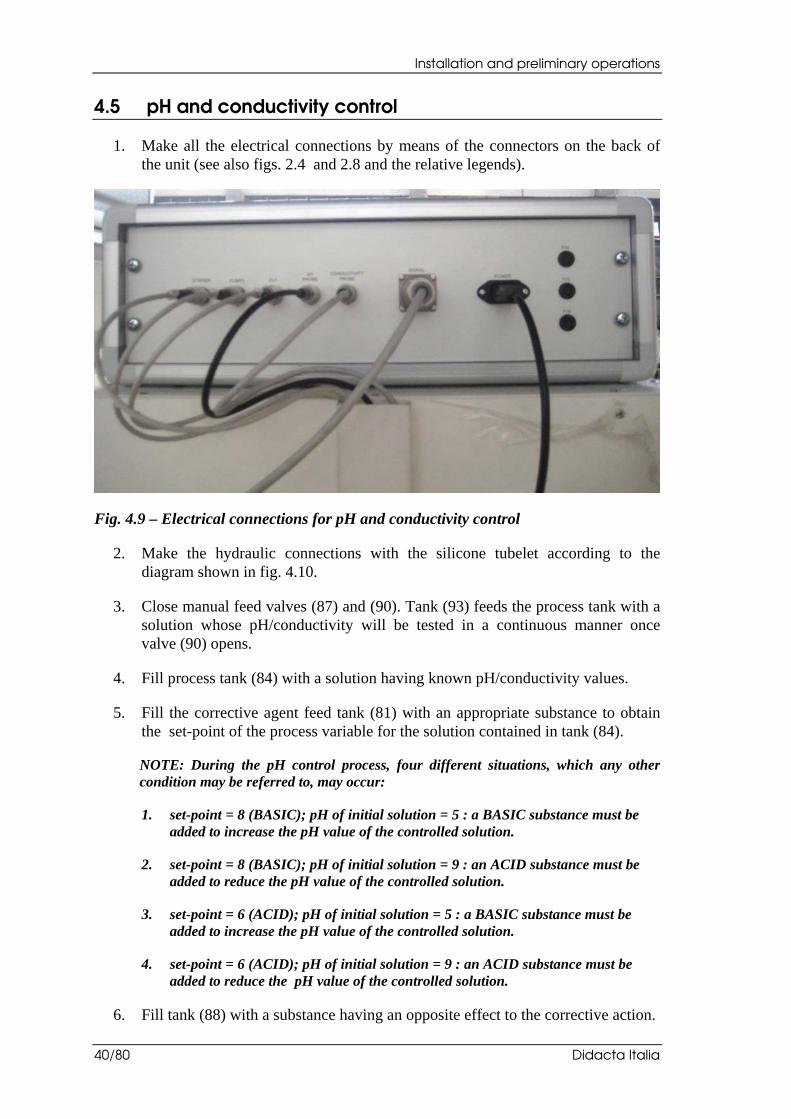
1. Make all the electrical connections by means of the connectors on the back of the unit (see also figs. 2.4 and 2.8 and the relative legends).
Fig. 4.9 – Electrical connections for pH and conductivity control
2. Make the hydraulic connections with the silicone tubelet according to the diagram shown in fig. 4.10.
3. Close manual feed valves (87) and (90). Tank (93) feeds the process tank with a solution whose pH/conductivity will be tested in a continuous manner once valve (90) opens.
4. Fill process tank (84) with a solution having known pH/conductivity values.
5. Fill the corrective agent feed tank (81) with an appropriate substance to obtain the set-point of the process variable for the solution contained in tank (84).
NOTE: During the pH control process, four different situations, which any other condition may be referred to, may occur:
1. set-point = 8 (BASIC); pH of initial solution = 5 : a BASIC substance must be added to increase the pH value of the controlled solution.
2. set-point = 8 (BASIC); pH of initial solution = 9 : an ACID substance must be added to reduce the pH value of the controlled solution.
3. set-point = 6 (ACID); pH of initial solution = 5 : a BASIC substance must be added to increase the pH value of the controlled solution.
4. set-point = 6 (ACID); pH of initial solution = 9 : an ACID substance must be added to reduce the pH value of the controlled solution.
6. Fill tank (88) with a substance having an opposite effect to the corrective action.
Chapter 4.
MPCT - User’s Manual 41/80
7. Place the pH/conductivity probe in its seat located in the cover of the process tank (84).
8. The same module can be used to control both the pH and the conductivity of the solution contained in process tank 84. The operating principle is the same in both processes. The only provision to be kept in mind when changing from one process to the other is to wash accurately the tanks and to change the probe, selecting the appropriate one and submerging it in the process tank. Washing the tanks and the probes is also required when, in using the module to control the pH of a solution, we go from a substance with basic pH to be acidified to a substance with acid pH to be basified. To ensure that they are emptied out completely, the tanks are fitted with discharge valves to be connected to the respective collection tanks. The tanks are also fitted with appropriate covers to facilitate the filling process.
9. Power the unit by means of the switch (1).
10. Press process selector (56) or (55): telltales (57) or (54) will light up to indicate that the module is ON.
11. Set to zero the speed potentiometers for pump P3 speed and solenoid valve 60 (14) and (10).
12. Set automatic/manual selector (9) to MAN.
13. Set selector (2) to “MINIREG”.
14. Set to ON the ON/OFF selectors for pump 3 and the solenoid valve (16) and (12).
15. By means of speed potentiometers (14) and (10) make sure that speed variations produced by the pump and the solenoid valve range from zero to 100% (values shown on display (4)9. Select the quantity to be viewed on display (4) by means of selector (5).
16. Set to OFF the ON/OFF selectors of pump 3 and the solenoid valve (16) and (12).
17. Conductivity and pH values can be read on instruments (18) and (19), respectively.
18. Set selector (9) to AUTOM.
19. Set selector (2) to PC (or to MINIREG if you plan to use the MiniReg external controller).
20. Set to ON the ON/OFF selectors of pump 3 and the solenoid valve (16) and (12).
21. Open valves 90 and 87.
22. Launch program MPCT/pH or MPCT/C and carry out process control using the soft keys that appear on the various screens.

Installation and preliminary operations
42/80 Didacta Italia
23. If you want to obtain a solution with a more homogeneous pH start the mixer by pressing switch (53): telltale (52) lights up to indicate that the module is ON.
NOTE: For proper unit operation, set solenoid valve opening value to 0 % or 100%. (Valve fully closed or fully open).

Chapter 4.
MPCT - User’s Manual 43/80
Fig. 4.10 – Hydraulic connections for conductivity/pH control

Installation and preliminary operations
44/80 Didacta Italia
Chapter 5.
MPCT - User’s Manual 45/80
5. Exercises
5.1 Exercise 1 — On-Off level control via software
Test execution modalities
1. Perform the initial operations listed in 4.1 and in particular make sure that:
• process selector (3) is pressed (telltale (20) lights up)
• control mode selector (2) is set to “PC”;
• graduated tank (74) is empty;
• the mode selector for the two pumps (9) is set to “AUTOM”;
• the start selectors for the two pumps (12) and (16) set to ON.
2. Launch the MPCT/L program.
3. Select File-New.
4. Select “On-Off Regulator” in the “Select Exercise Type” window and click OK.
5. Enter the operator’s name and your comments, if any, in the “Test Description” window and click OK.
6. In the “Set Up set-point” window, set:
• Function = DC
• Amplitude = 50%
• Offset = 50%
• Period= /
7. In the “On-Off Parameters” window, set:
• Hysteresis = 5%
• Open Time: 2 s
• Gain: 0.5
and click OK.
8. In the “Noise Setup” window, set:
• Function: DC (continuous noise)

Exercises
46/80 Didacta Italia
• Amplitude = 30 %
• Offset = 0 %
• Period= /
and click OK.
9. In the “Real Time Diagram” window make sure that noise is enabled, through the “enable” field contained in the “Noise” box.
10. Click the “Start” button to start the test.
11. Monitor system behaviour for a few minutes paying special attention to the effects of controller parameters.
12. Notice how the system reacts to different kinds of noise, e.g., z, square-wave or sinusoidal type noise, by changing its characteristics through the “Noise Setup” window that is recalled with the “Noise” button.
13. Evaluate separately the effects of the various parameters of the controller by changing them through the “On-Off Parameters” window opened with the “Param” button. Evaluate system reactions to changes in set-point values.
14. At the end of the test click “Stop” and “Cancel”.
15. Monitor samples of the signals involved in the test and their evolution over time through the File-Browse-Data and File-Browse-Diagram functions.
16. If desired, print the data and/or the diagrams.
17. If desired, save the data to the disc through File-Save
18. End the exercise with File-Close.
19. Empty out the tank using pump 2 in manual mode.
Chapter 5.
MPCT - User’s Manual 47/80
Test results
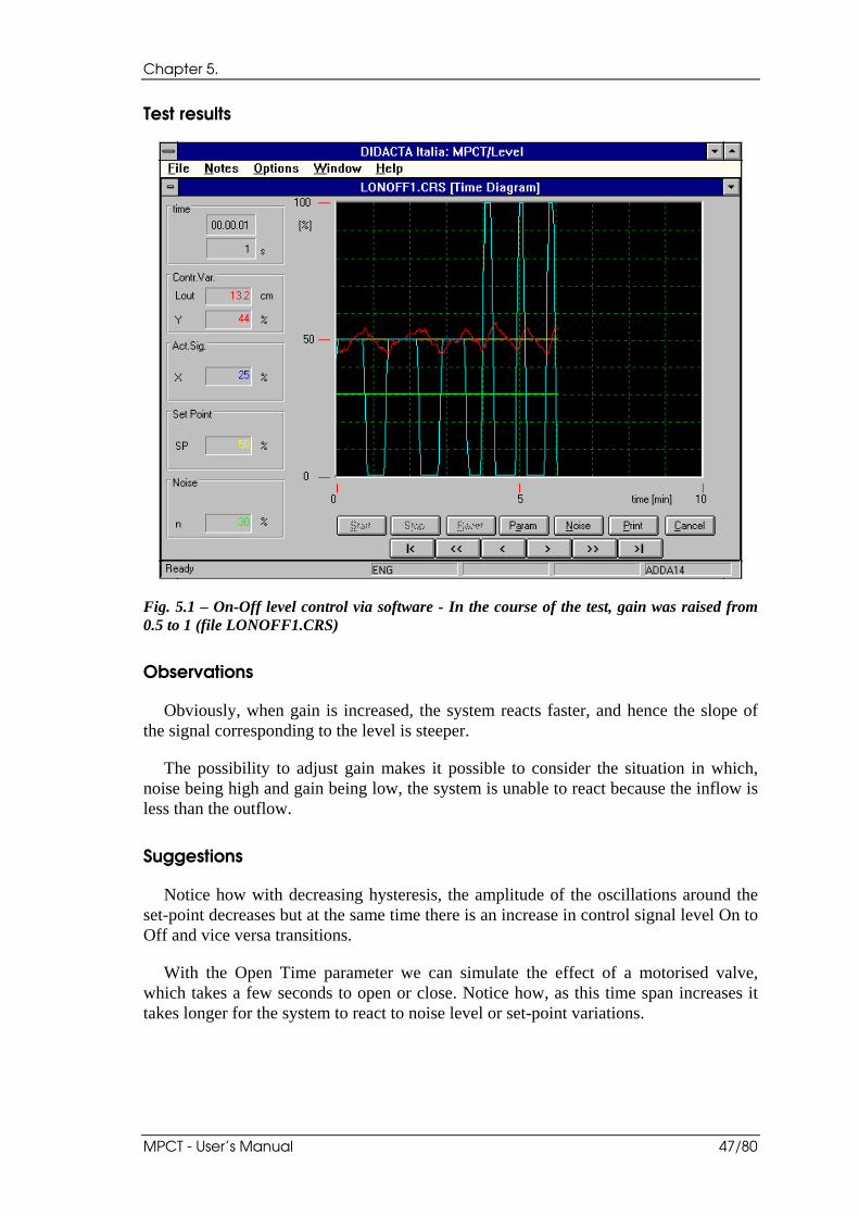
Fig. 5.1 – On-Off level control via software - In the course of the test, gain was raised from 0.5 to 1 (file LONOFF1.CRS)
Observations
Obviously, when gain is increased, the system reacts faster, and hence the slope of the signal corresponding to the level is steeper.
The possibility to adjust gain makes it possible to consider the situation in which, noise being high and gain being low, the system is unable to react because the inflow is less than the outflow.
Suggestions
Notice how with decreasing hysteresis, the amplitude of the oscillations around the set-point decreases but at the same time there is an increase in control signal level On to Off and vice versa transitions.
With the Open Time parameter we can simulate the effect of a motorised valve, which takes a few seconds to open or close. Notice how, as this time span increases it takes longer for the system to react to noise level or set-point variations.
Exercises
48/80 Didacta Italia
5.2 Exercise 2 — PID level control via software
Test execution modalities
1. Perform the initial operations listed in 4.1 and in particular make sure that:
• process selector (3) is pressed (telltale (20) lights up)
• control mode selector (2) is set to “PC”;
• graduated tank (74) is empty;
• the mode selector for the two pumps (9) is set to “AUTOM”;
• the start selectors for the two pumps (12) and (16) are set to ON.
2. Launch program MPCT/L.
3. Select File-New.
4. Select “PID Regulator” in the “Select Exercise Type” window and click OK.
5. Enter the operator’s name and your comments, if any, in the “Test Description” window and click OK.
6. In the “Set up set-point” window, set:
• Function = DC
• Amplitude = 50%
• Offset = 50%
• Period= /
7. In the “PID Parameters” window, set:
• Proportional Band = 286%
• Integrative Time = 0.5 min
• Derivative Time = 0 min
and click OK.
8. In the “Noise Setup” window, set:
• Function: DC (continuous noise)
• Amplitude = 30 %
• Offset = 0 %
Chapter 5.
MPCT - User’s Manual 49/80
• Period= /
and click OK.
9. Do not make any manual alignment, i.e., leave the control signal field in the “Manual Alignment” window set to 0 and click OK.
10. In the “Real Time Diagram” window, make sure that noise is enabled, through the “enable” field contained in the “Noise” box.
11. Click the “Start” button to start the test.
12. Monitor system behaviour for a few minutes paying special attention to the effects of controller parameters.
13. Notice how the system reacts to different kinds of noise, e.g., z, square-wave or sinusoidal type noise, by changing its characteristics through the “Noise Setup” window that is recalled with the “Noise” button.
14. Evaluate separately the effects of the various parameters of the controller by changing them through the “PID Parameters” window opened with the “Param” button. Evaluate system reactions to changes in set-point values.
15. At the end of the test click “Stop” and “Cancel”.
16. Monitor samples of the signals involved in the test and their evolution over time through the File-Browse-Data and File-Browse-Diagram functions.
17. If desired, print the data and/or the diagrams.
18. If desired, save the data to the disc through File-Save.
19. End the exercise with File-Close.
20. Empty out the graduated tank using pump 2 in manual mode.
Exercises
50/80 Didacta Italia
Test results
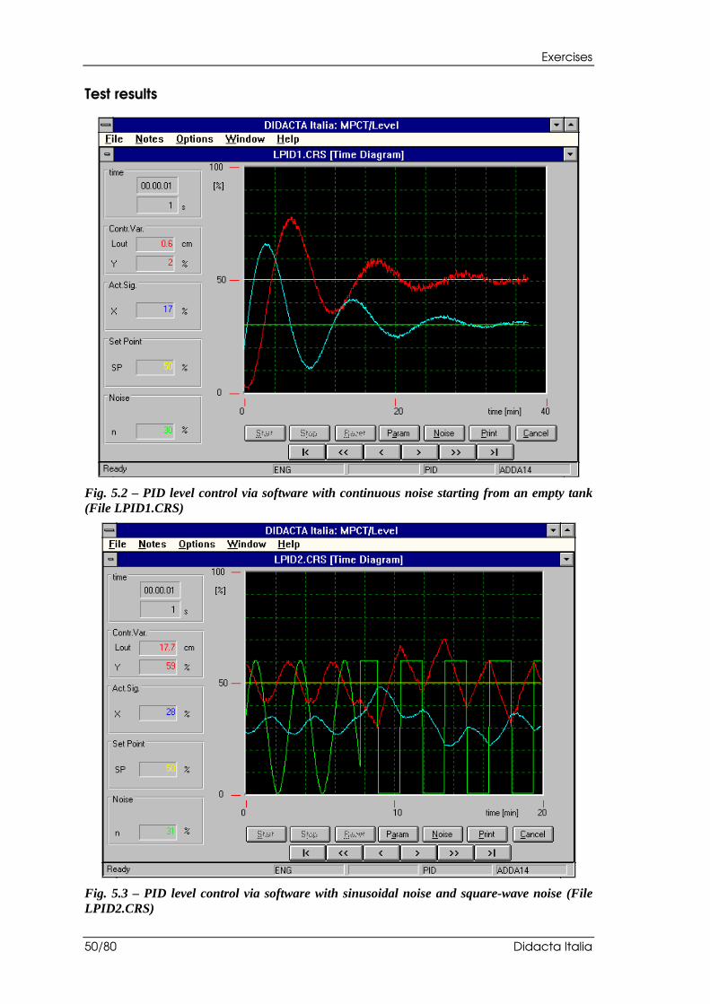
Fig. 5.2 – PID level control via software with continuous noise starting from an empty tank (File LPID1.CRS)
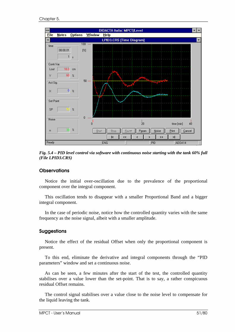
Fig. 5.3 – PID level control via software with sinusoidal noise and square-wave noise (File LPID2.CRS)
Chapter 5.
MPCT - User’s Manual 51/80
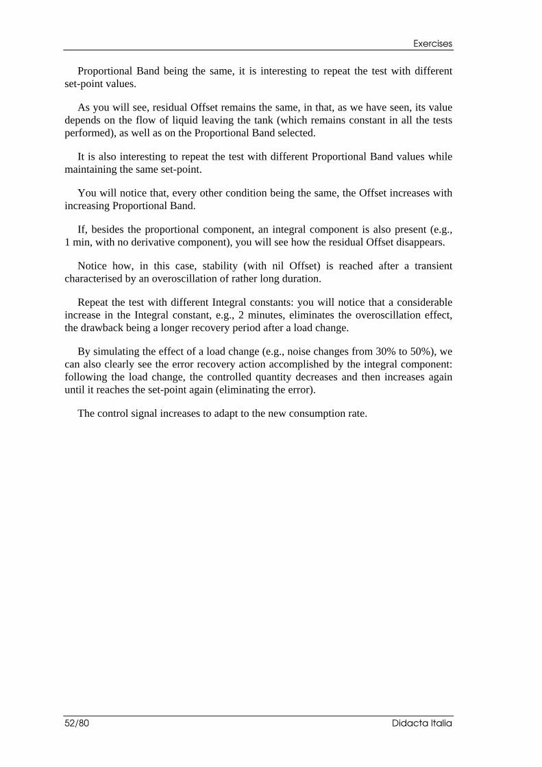
Fig. 5.4 – PID level control via software with continuous noise starting with the tank 60% full (File LPID3.CRS)
Observations
Notice the initial over-oscillation due to the prevalence of the proportional component over the integral component.
This oscillation tends to disappear with a smaller Proportional Band and a bigger integral component.
In the case of periodic noise, notice how the controlled quantity varies with the same frequency as the noise signal, albeit with a smaller amplitude.
Suggestions
Notice the effect of the residual Offset when only the proportional component is present.
To this end, eliminate the derivative and integral components through the “PID parameters” window and set a continuous noise.
As can be seen, a few minutes after the start of the test, the controlled quantity stabilises over a value lower than the set-point. That is to say, a rather conspicuous residual Offset remains.
The control signal stabilises over a value close to the noise level to compensate for the liquid leaving the tank.
Exercises
52/80 Didacta Italia
Proportional Band being the same, it is interesting to repeat the test with different set-point values.
As you will see, residual Offset remains the same, in that, as we have seen, its value depends on the flow of liquid leaving the tank (which remains constant in all the tests performed), as well as on the Proportional Band selected.
It is also interesting to repeat the test with different Proportional Band values while maintaining the same set-point.
You will notice that, every other condition being the same, the Offset increases with increasing Proportional Band.
If, besides the proportional component, an integral component is also present (e.g., 1 min, with no derivative component), you will see how the residual Offset disappears.
Notice how, in this case, stability (with nil Offset) is reached after a transient characterised by an overoscillation of rather long duration.
Repeat the test with different Integral constants: you will notice that a considerable increase in the Integral constant, e.g., 2 minutes, eliminates the overoscillation effect, the drawback being a longer recovery period after a load change.
By simulating the effect of a load change (e.g., noise changes from 30% to 50%), we can also clearly see the error recovery action accomplished by the integral component: following the load change, the controlled quantity decreases and then increases again until it reaches the set-point again (eliminating the error).
The control signal increases to adapt to the new consumption rate.
Chapter 5.
MPCT - User’s Manual 53/80
5.3 Exercise 3 — PID level control with MiniReg controller
Introductory considerations
This exercise is performed with the MINIREG electronic controller available as an option; in this case too, the CRS software is used to observe the behaviour of the system and to transmit the set-point signal to the external controller.
For details on the operation of the MiniReg, the reader is referred to the relative documentation; keep in mind that before it can be used selector (2) must be set to MiniReg.
The MiniReg is able to perform PID or On-Off control, enabling the operator to define the values to be assigned to the fundamental parameters; a special functional feature of the MiniReg is the automatic determination of the optimal values for the PID parameters.
The exercise consists of using the MiniReg in this operating mode and to analyse system behaviour through the CRS software. Moreover, it is interesting to have the MiniReg determine the optimal values of the PID parameters and compare them with the values set with the CRS software during the previous exercises.
Test execution modalities
1. Check the electrical connections relating to the power supply and the signals of the MiniReg and turn on the MiniReg.
2. Perform the initial operations listed in 4.1 and in particular make sure that:
• process selector (3) is pressed (telltale (20) lights up)
• control mode selector (2) is set to “PC”;
• graduated tank (74) is empty;
• the mode selector for the two pumps (9) is set to “AUTOM”;
• the start selectors for the two pumps (12) and (16) are set to ON.
3. Launch program MPCT/L.
4. Select File-New.
5. Select “Ext. Regulator” in the “Select Exercise Type” window and click OK.
6. Enter the operator’s name and your comments, if any, in the “Test Description” window and click OK.
7. In the “Ext. Regulator Parameters” window, set:
• set-point = 50%
Exercises
54/80 Didacta Italia
and click OK.
8. By pressing the REM key, program the MiniReg in “Remote” mode to accept the set-point from the PC.
9. In the “Noise Setup” window, set:
• Function: DC (continuous noise)
• Amplitude = 30 %
• Offset = 0 %
and click OK.
10. In the “Real Time Diagram” window make sure that noise is enabled, through the “enable” field contained in the “Noise” box.
11. Click the “Start” button to start the test.
12. Set selector (2) to “MiniReg”.
13. Activate the “Self Tuning” function of the MiniReg according to the instructions provided in the MiniReg Manual.
14. Wait a few minutes so that the controller may interact with the process making it possible to determine the most appropriate control parameters.
15. Monitor system behaviour for a few minutes and wait until it stabilises.
16. Notice how the system reacts to different kinds of noise, e.g., z, square-wave or sinusoidal type noise, by changing its characteristics through the “Noise Setup” window that is recalled with the “Noise” button.
17. Notice how the system reacts to changes in set-point level by adjusting the set-point values in the “PID Parameters” window opened with the “Param” button.
18. Determine PID control parameters from the MiniReg.
19. At the end of the test click “Stop” and “Cancel”.
20. Monitor samples of the signals involved in the test and their evolution over time through functions File-Browse-Data and File-Browse-Diagram.
21. If desired, print the data and/or the diagrams.
22. If desired, save the data to the disc through File-Save.
23. End the exercise with File-Close.
24. Empty out the graduated tank using pump 2 in manual mode.
Chapter 5.
MPCT - User’s Manual 55/80
Test results
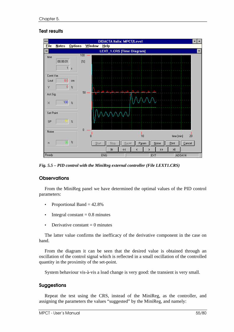
Fig. 5.5 – PID control with the MiniReg external controller (File LEXT1.CRS)
Observations
From the MiniReg panel we have determined the optimal values of the PID control parameters:
• Proportional Band = 42.8%
• Integral constant = 0.8 minutes
• Derivative constant = 0 minutes
The latter value confirms the inefficacy of the derivative component in the case on hand.
From the diagram it can be seen that the desired value is obtained through an oscillation of the control signal which is reflected in a small oscillation of the controlled quantity in the proximity of the set-point.
System behaviour vis-à-vis a load change is very good: the transient is very small.
Suggestions
Repeat the test using the CRS, instead of the MiniReg, as the controller, and assigning the parameters the values “suggested” by the MiniReg, and namely:
Exercises
56/80 Didacta Italia
• Proportional Band = 43%
• Integral constant = 0.8 minutes
• Derivative constant = 0 minutes
Following the instructions provided in Exercise 2, you will notice that the control action behaves much same way as with the MiniReg, but control signal oscillations are much smaller.
Though the PID parameters are the same, in fact, the two control techniques in question are completely different: one is analog and the other is digital. The digital simulation of an analog system, which, as is known, is obtained through the z transform, in fact, has inherent limits due to system discretisation.
Chapter 5.
MPCT - User’s Manual 57/80
5.4 Exercise 4 — PID flow control via software
Test execution modalities
1. Perform the initial operations listed in 4.2 and in particular make sure that:
• process selector (43) is pressed ( telltale (42) lights up)
• control mode selector (2) is set to “PC”;
• the mode selector for the two pumps (9) is set to “AUTOM”;
• the start selectors for the two pumps (12) and (16) are set to ON.
2. Launch program MPCT/F.
3. Select File-New.
4. Select “PID Regulator” in the “Select Exercise Type” and click OK.
5. Enter the operator’s name and your comments, if any, in the “Test Description” window and click OK.
6. In the “Set Up set-point” window, set:
• Function = DC
• Amplitude = 50%
• Offset = 50%
• Period= /
7. In the “PID Parameters” window, set:
• Proportional Band = 150%
• Integrative Time = 0.5 min
• Derivative Time = 0 min
and click OK.
8. In the “Noise Setup” window, set:
• Function: DC (continuous noise)
• Amplitude = 15 %
• Offset = 0 %
• Period= /
Exercises
58/80 Didacta Italia
and click OK.
9. Do not make any manual alignment, i.e., leave the control signal field in the “Manual Alignment” window set to 0 and click OK.
10. In the “Real Time Diagram” window make sure that noise is enabled, through the “enable” field contained in the “Noise” box.
11. Click the “Start” button to start the test.
12. Monitor system behaviour for a few minutes paying special attention to the effects of controller parameters.
13. Notice how the system reacts to different kinds of noise, e.g., z, square-wave or sinusoidal type noise, by changing its characteristics through the “Noise Setup” window that is recalled with the “Noise” button.
14. Evaluate separately the effects of the various parameters of the controller by changing them through the “PID Parameters” window opened with the “Param” button. Evaluate system reactions to changes in set-point values.
15. At the end of the test click “Stop” and “Cancel”.
16. Monitor samples of the signals involved in the test and their evolution over time through the File-Browse-Data and File-Browse-Diagram functions.
17. If desired, print the data and/or the diagrams.
18. If desired, save the data to the disc through File-Save.
19. End the exercise with File-Close.
20. Empty out the tank using pump 2 in manual mode.

Chapter 5.
MPCT - User’s Manual 59/80
Test results
Fig. 5.6 – PID flow control - During the test, noise has been raised from 15% to 10% and 25% and the set-point from 35% to 50% (file FPID1.CRS)
Fig. 5.7 – PID flow control with P-Band=50% and sinusoidal noise - During the test, the set-point has been raised from 35% to 30% (file FPID2.CRS)
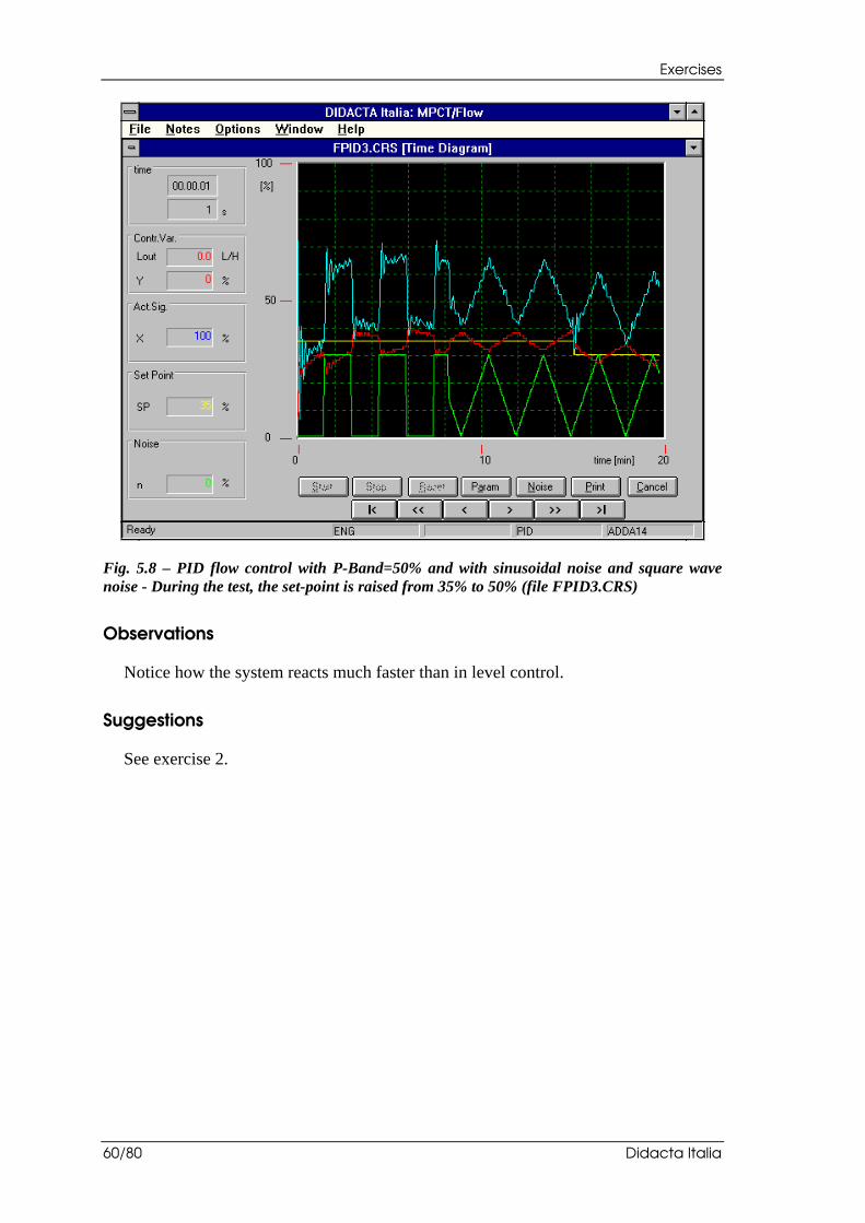
Exercises
60/80 Didacta Italia
Fig. 5.8 – PID flow control with P-Band=50% and with sinusoidal noise and square wave noise - During the test, the set-point is raised from 35% to 50% (file FPID3.CRS)
Observations
Notice how the system reacts much faster than in level control.
Suggestions
See exercise 2.
Chapter 5.
MPCT - User’s Manual 61/80
5.5 Exercise 5 — PID pressure control via software
Test execution modalities
1. Perform the initial operations listed in 4.3 and in particular make sure that:
• process selector (3) is pressed (telltale (20) lights up)
• control mode selector (2) is set to “PC”;
• graduated tank (74) is empty;
• the mode selector for the two pumps (9) is set to “AUTOM”;
• the start selectors for the two pumps (12) and (16) are set to ON.
2. Launch program MPCT/P.
3. Select File-New.
4. Select “PID Regulator” in the “Select Exercise Type” window and click OK.
5. Enter the operator’s name and your comments, if any, in the “Test Description” window and click OK.
6. In the “Set Up set-point” window, set:
• Function = DC
• Amplitude = 50%
• Offset = 50%
• Period= /
7. In the “PID Parameters” window, set:
• Proportional Band = 286%
• Integrative Time = 0.5 min
• Derivative Time = 0 min
and click OK.
8. In the “Noise Setup” window, set:
• Function: DC (continuous noise)
• Amplitude = 10 %
• Offset = 0 %
Exercises
62/80 Didacta Italia
• Period= /
and click OK.
9. Do not make any manual alignment, i.e., leave the control signal field in the “Manual Alignment” window set to 0 and click OK.
10. In the “Real Time Diagram” window make sure that noise is enabled, through the “enable” field contained in the “Noise” box.
11. Click the “Start” button to start the test.
12. Monitor system behaviour for a few minutes paying special attention to the effects of controller parameters.
13. Notice how the system reacts to different kinds of noise, e.g., z, square-wave or sinusoidal type noise, by changing its characteristics through the “Noise Setup” window that is recalled with the “Noise” button.
14. Evaluate separately the effects of the various parameters of the controller by changing them through the “PID Parameters” window opened with the “Param” button. Evaluate system reactions to changes in set-point values.
15. At the end of the test click “Stop” and “Cancel”.
16. Monitor samples of the signals involved in the test and their evolution over time through the File-Browse-Data and File-Browse-Diagram functions.
17. If desired, print the data and/or the diagrams.
18. If desired, save the data to the disc through File-Save.
19. End the exercise with File-Close.
20. Empty out the graduated tank using pump 2 in manual mode.
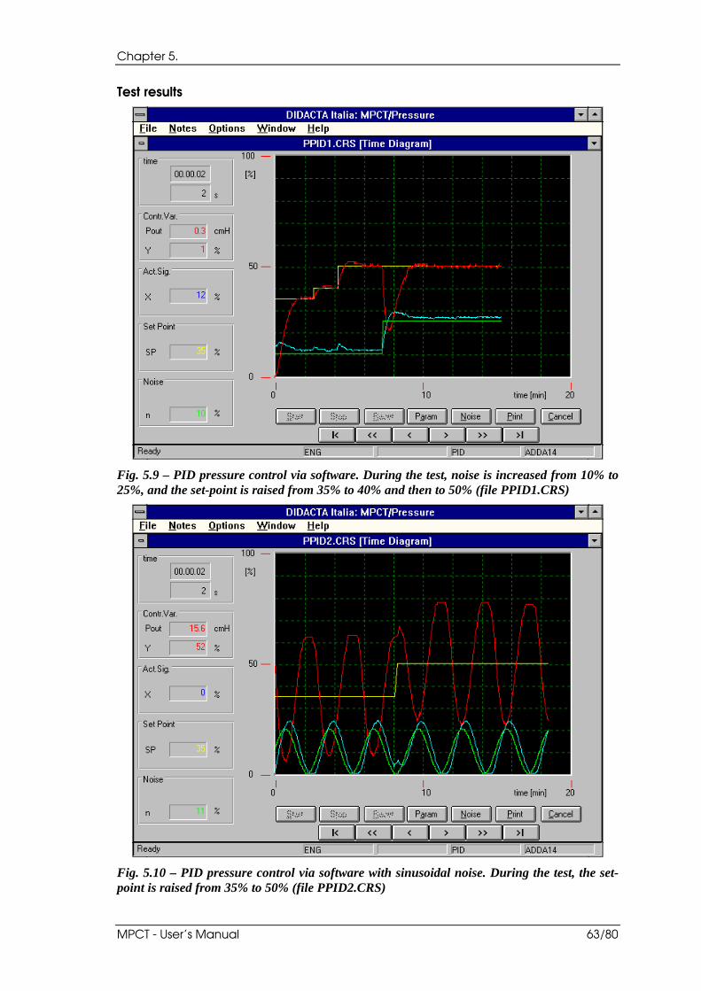
Chapter 5.
MPCT - User’s Manual 63/80
Test results
Fig. 5.9 – PID pressure control via software. During the test, noise is increased from 10% to 25%, and the set-point is raised from 35% to 40% and then to 50% (file PPID1.CRS)
Fig. 5.10 – PID pressure control via software with sinusoidal noise. During the test, the set-point is raised from 35% to 50% (file PPID2.CRS)
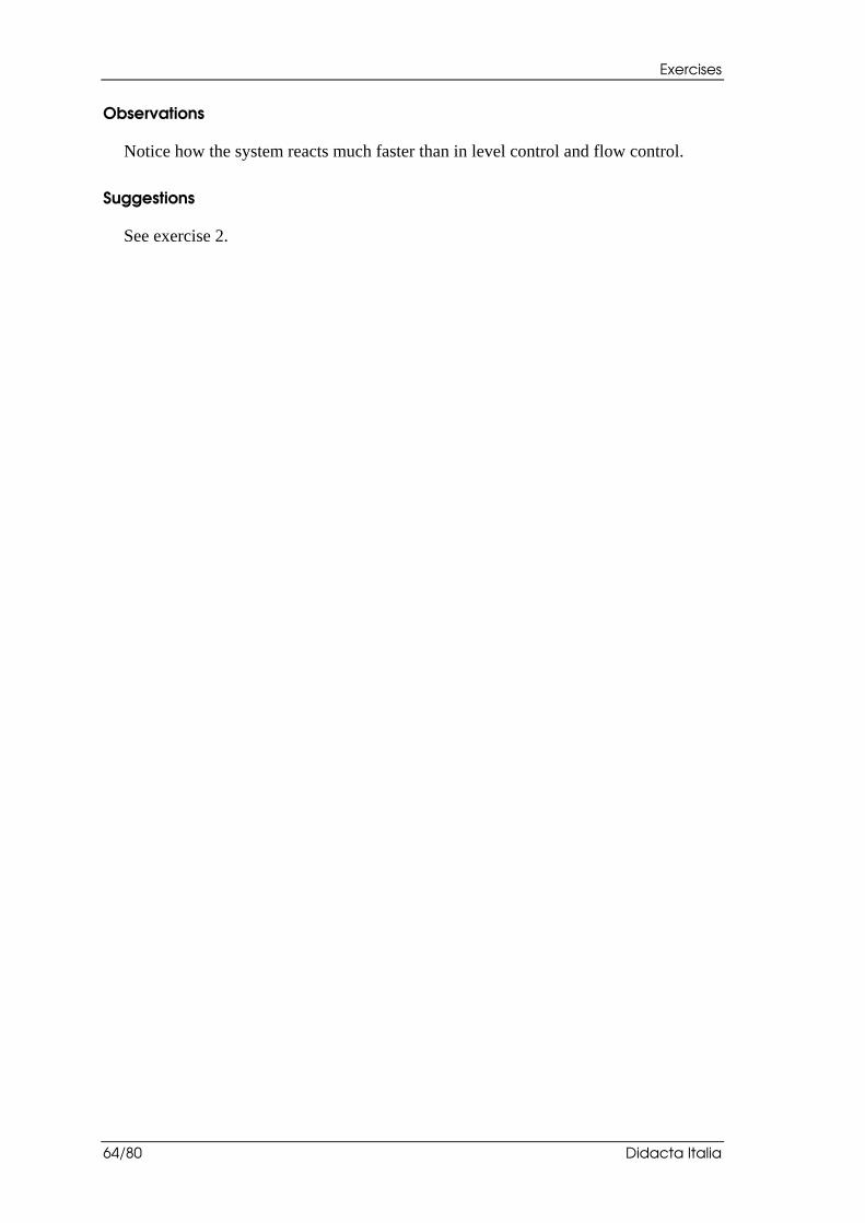
Exercises
64/80 Didacta Italia
Observations
Notice how the system reacts much faster than in level control and flow control.
Suggestions
See exercise 2.
Chapter 5.
MPCT - User’s Manual 65/80
5.6 Exercise 6 — PID temperature control via software
Test execution modalities
1. Perform the initial operations listed in 4.4 and in particular make sure that:
• process selector (40) is pressed (telltale (39) lights up)
• control mode selector (2) is set to “PC”;
• the heater resistance switch (38) is set to ON and tank (69) contains sufficiently warm water;
• tank (80) contains cold water;
• the mode selector for the two pumps (9) is set to “AUTOM”;
• the start selectors for the two pumps (12) and (16) are set to ON.
2. Launch program MPCT/T.
3. Select File-New.
4. Select “PID Regulator” in the “Select Exercise Type” window and click OK.
5. Enter the operator’s name and your comments, if any, in the “Test Description” window and click OK.
6. In the “Set Up set-point” window, set:
• Function = DC
• Amplitude = 50%
• Offset = 50%
• Period= /
7. In the “PID Parameters” window, set:
• Proportional Band = 286%
• Integrative Time = 0.5 min
• Derivative Time = 0 min
and click OK.
8. In the “Noise Setup” window, set:
• Function: DC (continuous noise)
Exercises
66/80 Didacta Italia
• Amplitude = 10 %
• Offset = 0 %
• Period= /
and click OK.
9. Do not make any manual alignment, i.e., leave the control signal field in the “Manual Alignment” window set to 0 and click OK.
10. In the “Real Time Diagram” window make sure that noise is enabled, through the “enable” field contained in the “Noise” box.
11. Click the “Start” button to start the test.
12. Monitor system behaviour for a few minutes paying special attention to the effects of controller parameters.
13. Notice how the system reacts to different kinds of noise, e.g., z, square-wave or sinusoidal type noise, by changing its characteristics through the “Noise Setup” window that is recalled with the “Noise” button.
14. Evaluate separately the effects of the various parameters of the controller by changing them through the “PID Parameters” window opened with the “Param” button. Evaluate system reactions to changes in set-point values.
15. At the end of the test click “Stop” and “Cancel”.
16. Monitor samples of the signals involved in the test and their evolution over time through the File-Browse-Data and File-Browse-Diagram functions.
17. If desired, print the data and/or the diagrams.
18. If desired, save the data to the disc through File-Save.
19. End the exercise with File-Close.
20. Empty out the hot water tank (69).
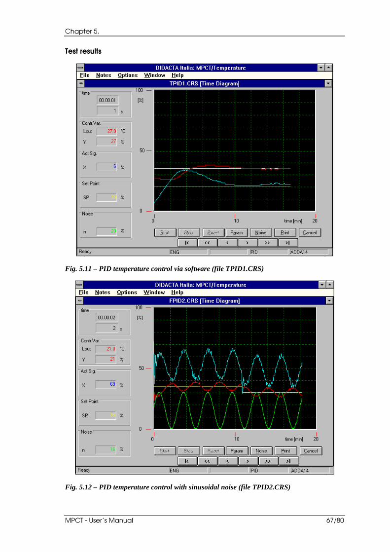
Chapter 5.
MPCT - User’s Manual 67/80
Test results
Fig. 5.11 – PID temperature control via software (file TPID1.CRS)
Fig. 5.12 – PID temperature control with sinusoidal noise (file TPID2.CRS)
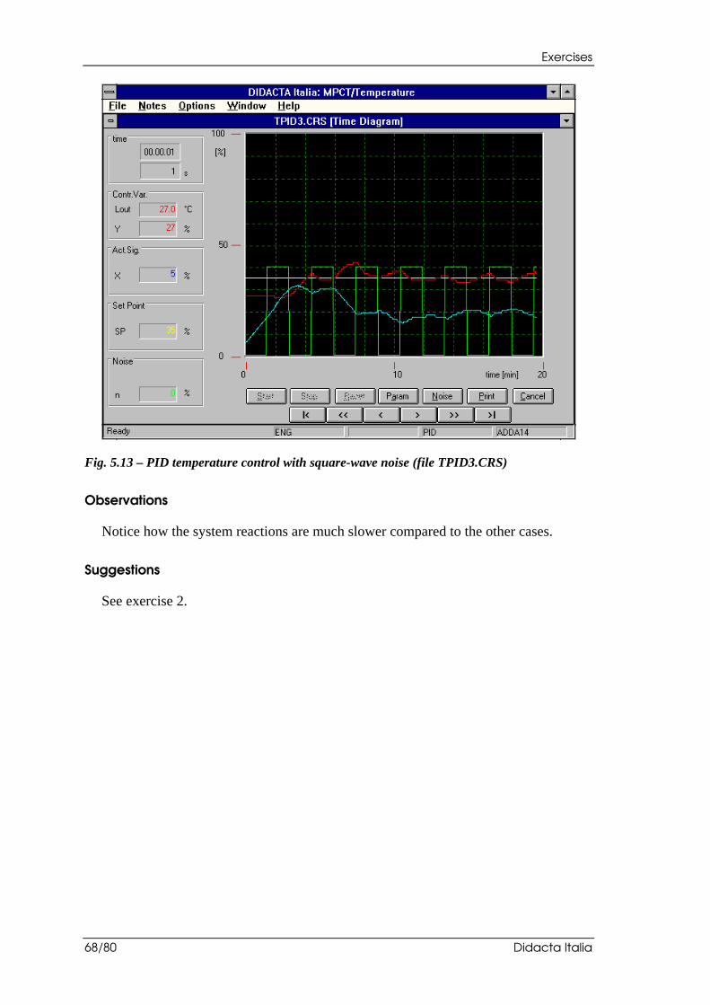
Exercises
68/80 Didacta Italia
Fig. 5.13 – PID temperature control with square-wave noise (file TPID3.CRS)
Observations
Notice how the system reactions are much slower compared to the other cases.
Suggestions
See exercise 2.
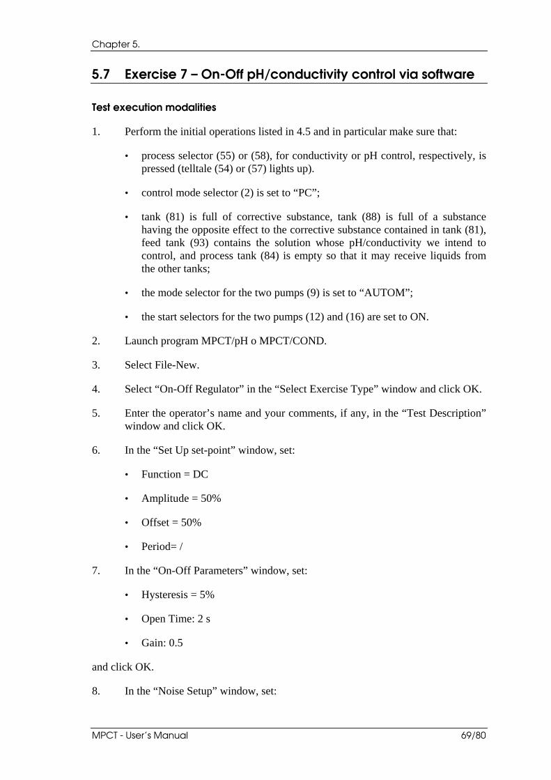
Chapter 5.
MPCT - User’s Manual 69/80
5.7 Exercise 7 — On-Off pH/conductivity control via software
Test execution modalities
1. Perform the initial operations listed in 4.5 and in particular make sure that:
• process selector (55) or (58), for conductivity or pH control, respectively, is pressed (telltale (54) or (57) lights up).
• control mode selector (2) is set to “PC”;
• tank (81) is full of corrective substance, tank (88) is full of a substance having the opposite effect to the corrective substance contained in tank (81), feed tank (93) contains the solution whose pH/conductivity we intend to control, and process tank (84) is empty so that it may receive liquids from the other tanks;
• the mode selector for the two pumps (9) is set to “AUTOM”;
• the start selectors for the two pumps (12) and (16) are set to ON.
2. Launch program MPCT/pH o MPCT/COND.
3. Select File-New.
4. Select “On-Off Regulator” in the “Select Exercise Type” window and click OK.
5. Enter the operator’s name and your comments, if any, in the “Test Description” window and click OK.
6. In the “Set Up set-point” window, set:
• Function = DC
• Amplitude = 50%
• Offset = 50%
• Period= /
7. In the “On-Off Parameters” window, set:
• Hysteresis = 5%
• Open Time: 2 s
• Gain: 0.5
and click OK.
8. In the “Noise Setup” window, set:
Exercises
70/80 Didacta Italia
• Function: DC (continuous noise)
• Amplitude = 100 %
• Offset = 0 %
• Period= /
and click OK.
NOTE: For proper unit operation, set solenoid valve opening value to 0 % or 100%. (Valve fully closed or fully open).
9. In the “Real Time Diagram” window make sure that noise is enabled, through the “enable” field contained in the “Noise” box.
10. Click the “Start” button to start the test.
11. Monitor system behaviour for a few minutes paying special attention to the effects of controller parameters.
12. Evaluate separately the effects of the various parameters of the controller by changing them through the “On-Off Parameters” window opened with the “Param” button. Evaluate system reactions to changes in set-point values.
13. At the end of the test click “Stop” and “Cancel”.
14. Monitor samples of the signals involved in the test and their evolution over time through the File-Browse-Data and File-Browse-Diagram functions.
15. If desired, print the data and/or the diagrams.
16. If desired, save the data to the disc through File-Save
17. End the exercise with File-Close.
18. Empty out the tank using pump 2 in manual mode.
Test results
Observations
Obviously, when gain is increased, the system reacts faster, and hence the slope of the signal corresponding to the level is steeper.
The possibility to adjust gain makes it possible to consider the situation in which, noise being high and gain being low, the system is unable to react because the amount of corrective substance flowing in is less than the inflow of the substance having the opposite effect (noise).
Chapter 5.
MPCT - User’s Manual 71/80
Suggestions
Notice how with decreasing hysteresis, the amplitude of the oscillations around the set-point decreases but at the same time there is an increase in control signal level On to Off and vice versa transitions.
With the Open Time parameter we can simulate the effect of a motorised valve, which takes a few seconds to open or close. Notice how, as this time span increases it takes longer for the system to react to noise level or set-point variations.
Exercises
72/80 Didacta Italia
5.8 Exercise 8 — PID pH/conductivity control via software
Test execution modalities
1. Perform the initial operations listed in 4.5 and in particular make sure that:
• process selector (55) or (58), for conductivity or pH control, respectively, is pressed (telltale (54) or (57) lights up).
• control mode selector (2) is set to “PC”;
• tank (81) is full of corrective substance, tank (88) is full of a substance having the opposite effect to the corrective substance contained in tank (81), feed tank (93) contains the solution whose pH/conductivity values we intend to control, and process tank (84) is empty so that it may receive liquids from the other tanks;
• the mode selector for the two pumps (9) is set to “AUTOM”;
• the start selectors for the two pumps (12) and (16) are set to ON.
2. Launch program MPCT/pH o MPCT/COND.
3. Select File-New.
4. Select “PID Regulator” in the “Select Exercise Type” window and click OK.
5. Enter the operator’s name and your comments, if any, in the “Test Description” window and click OK.
6. In the “Set Up set-point” window, set:
• Function = DC
• Amplitude = 50%
• Offset = 50%
• Period= /
7. In the “PID Parameters” window, set:
• Proportional Band = 286%
• Integrative Time = 0.5 min
• Derivative Time = 0 min
and click OK.
8. In the “Noise Setup” window, set:
Chapter 5.
MPCT - User’s Manual 73/80
• Function: DC (continuous noise)
• Amplitude = 100 %
• Offset = 0 %
• Period= /
and click OK.
NOTE: For proper unit operation, set solenoid valve opening value to 0 % or 100%. (Valve fully closed or fully open).
9. Do not make any manual alignment, i.e., leave the control signal field in the “Manual Alignment” window set to 0 and click OK.
10. In the “Real Time Diagram” window make sure that noise is enabled, through the “enable” field contained in the “Noise” box.
11. Click the “Start” button to start the test.
12. Monitor system behaviour for a few minutes paying special attention to the effects of controller parameters.
13. Evaluate separately the effects of the various parameters of the controller by changing them through “PID Parameters” window recalled with the “Param” button. Evaluate system reactions to changes in set-point values.
14. At the end of the test click “Stop” and “Cancel”.
15. Monitor samples of the signals involved in the test and their evolution over time through the File-Browse-Data and File-Browse-Diagram functions.
16. If desired, print the data and/or the diagrams.
17. If desired, save the data to the disc through File-Save.
18. End the exercise with File-Close.
19. The same module may be used for the control of the pH and the conductivity of the solution contained in process tank 84. The operating principle is the same in both processes. The only provision to be kept in mind when changing from one process to the other is to wash accurately the tanks and to change the probe, selecting the appropriate one and submerging it in the process tank. Washing the tanks and the probes is also required when, in using the module to control the pH of a solution, we go from a substance with basic pH to be acidified to a substance with acid pH to be basified. To ensure that they are emptied out completely, the tanks are fitted with discharge valves to be connected to the respective collection tanks. The tanks are also fitted with appropriate covers to facilitate the filling process.
Exercises
74/80 Didacta Italia
Test results
Observations
Notice the initial over-oscillation due to the prevalence of the proportional component over the integral component.
This oscillation tends to disappear with a smaller Proportional Band and a bigger integral component.
In the case of periodic noise, notice how the controlled quantity varies with the same frequency as the noise signal, albeit with a smaller amplitude.
Suggestions
Notice the effect of residual Offset when only the proportional component is present.
To this end, eliminate the derivative and integral components through the “PID parameters” window and set a continuous noise.
As can be seen, a few minutes after the start of the test, the controlled quantity stabilises over a value lower than the set-point. That is to say, a rather conspicuous residual Offset remains.
The control signal stabilises over a value close to the noise level to compensate for the liquid leaving the tank.
The Proportional Band being the same, it is interesting to repeat the test with different set-point values.
As you will see, residual Offset remains the same, in that, as we have seen, its value depends on the flow of liquid leaving the tank (which remains constant in all the tests performed), as well as on the Proportional Band selected.
It is also interesting to repeat the test with different Proportional Band values while maintaining the same set-point.
You will notice that, every other condition being the same, the Offset increases with increasing Proportional Band.
If, besides the proportional component, an integral component is also present (e.g., 1 min, with no derivative component), you will see how the residual Offset disappears.
Notice how, in this case, stability (with nil Offset) is reached after a transient characterised by an overoscillation of rather long duration.
Repeat the test with different Integral constants: you will notice that a considerable increase in the Integral constant, e.g., 2 minutes, eliminates the overoscillation effect, the drawback being a longer recovery period after a load change.
Chapter 5.
MPCT - User’s Manual 75/80
By simulating the effect of a load change we can also clearly see the error recovery action accomplished by the integral component: following the load change, the controlled quantity decreases and then increases again until it reaches the set-point again (eliminating the error).
The control signal increases to adapt to the new consumption rate.
Exercises
76/80 Didacta Italia
5.9 Exercise 9 — PID pH/Conductivity control with the MiniReg
Introductory considerations
This exercise is performed with the MINIREG electronic controller available as an option; in this case too, the CRS software is used to observe the behaviour of the system and to transmit the set-point signal to the external controller.
For details on the operation of the MiniReg, the reader is referred to the relative documentation; keep in mind that before it can be used selector (2) must be set to MiniReg.
The MiniReg is able to perform PID or On-Off control, enabling the operator to define the values to be assigned to the fundamental parameters; a special functional feature of the MiniReg is the automatic determination of the optimal values for the PID parameters.
The exercise consists of using the MiniReg in this operating mode and to analyse system behaviour through the CRS software. Moreover, it is interesting to have the MiniReg determine the optimal values of the PID parameters and compare them with the values set with the CRS software during the previous exercises.
Test execution modalities
1. Check the electrical connections relating to the power supply and the signals of the MiniReg, and turn on the MiniReg.
2. Perform the initial operations listed in 4.5 and in particular make sure that:
• process selector (55) or (58), for conductivity or pH control, respectively, is pressed (telltale (54) or (57) lights up).
• control mode selector (2) is set to “PC”;
• tank (81) is full of corrective substance, tank (88) is full of a substance having the opposite effect to the corrective substance contained in tank (81), feed tank (93) contains the solution whose pH/conductivity we intend to control, and process tank (84) is empty so that it may receive liquids from the other tanks;
• the mode selector for the two pumps (9) is set to “AUTOM”;
• the start selectors for the two pumps (12) and (16) are set to ON.
3. Launch program MPCT/pH o MPCT/COND.
4. Select File-New.
5. Select “Ext. Regulator” in the “Select Exercise Type” window and click OK.
Chapter 5.
MPCT - User’s Manual 77/80
6. Enter the operator’s name and your comments, if any, in the “Test Description” window and click OK.
7. In the “Ext. Regulator Parameters” window, set:
• set-point = 50%
and click OK.
8. By pressing the REM key, program the MiniReg in “Remote” mode to accept the set-point from the PC.
9. In the “Noise Setup” window, set:
• Function: DC (continuous noise)
• Amplitude = 100 %
• Offset = 0 %
and click OK.
NOTE: For proper unit operation, set solenoid valve opening value to 0 % or 100%. (Valve fully closed or fully open).
10. In the “Real Time Diagram” window make sure that noise is enabled, through the “enable” field contained in the “Noise” box.
11. Click the “Start” button to start the test.
12. Set selector (2) to “MiniReg”.
13. Activate the “Self Tuning” function of the MiniReg according to the instructions provided in the MiniReg Manual.
14. Wait a few minutes so that the controller may interact with the process making it possible to determine the most appropriate control parameters.
15. Monitor system behaviour for a few minutes and wait until it stabilises.
16. Notice how the system reacts to changes in set-point level by adjusting the set-point values in the “PID Parameters” window opened with the “Param” button.
17. Determine PID control parameters from the MiniReg.
18. At the end of the test click “Stop” and “Cancel”.
19. Monitor samples of the signals involved in the test and their evolution over time through functions File-Browse-Data and File-Browse-Diagram.
20. If desired, print the data and/or the diagrams.
21. If desired, save the data to the disc through File-Save.
Exercises
78/80 Didacta Italia
22. End the exercise with File-Close.
23. The same module may be used for the control of the pH and the conductivity of the solution contained in process tank 84. The operating principle is the same in both processes. The only provision to be kept in mind when changing from one process to the other is to wash accurately the tanks and to change the probe, selecting the appropriate one and submerging it in the process tank. Washing the tanks and the probes is also required when, in using the module to control the pH of a solution, we go from a substance with basic pH to be acidified to a substance with acid pH to be basified. To ensure that they are emptied out completely, the tanks are fitted with discharge valves to be connected to the respective collection tanks. The tanks are also fitted with appropriate covers to facilitate the filling process.
Test results
Observations
From the MiniReg panel we have determined the optimal values of the PID control parameters:
• Proportional Band = 42.8%
• Integral constant = 0.8 minutes
• Derivative constant = 0 minutes
The latter value confirms the inefficacy of the derivative component in the case on hand.
From the diagram, it can be seen that the desired value is obtained through an oscillation of the control signal which is reflected in a small oscillation of the controlled quantity in the proximity of the set-point.
System behaviour vis-à-vis a load change is very good: the transient is very small.
Suggestions
Repeat the test using the CRS, instead of the MiniReg, as the controller, and assigning the parameters the values “suggested” by the MiniReg, and namely:
• Proportional Band = 43%
• Integral constant = 0.8 minutes
• Derivative constant = 0 minutes
Following the instructions provided in Exercise 2, you will notice that the control action behaves much same way as with the MiniReg, but control signal oscillations are much smaller.

Chapter 5.
MPCT - User’s Manual 79/80
Though the PID parameters are the same, in fact, the two control techniques in question are completely different: one is analog and the other is digital. The digital simulation of an analog system, which, as is known, is obtained through the z transform, in fact, has inherent limits due to system discretisation.

Exercises
80/80 Didacta Italia