Efficient Ehrlich–Aberth iteration for findingintersections of interpolating polynomials and rational

functions

Leonardo Robola,1, Raf Vandebrilb

aISTI, Area della ricerca CNR, Via G. Moruzzi 1, 56124 Pisa, Italy.bDepartment of Computer Science, KU Leuven, Celestijnenlaan 200A, 3001 Heverlee,

Belgium.

Abstract

We analyze the problem of carrying out an efficient iteration to approximate theeigenvalues of some rank structured pencils obtained as linearization of sums ofpolynomials and rational functions expressed in (possibly different) interpolationbases. The class of linearizations that we consider has been introduced by Robol,Vandebril and Van Dooren in [17]. We show that a traditional QZ iteration onthe pencil is both asymptotically slow (since it is a cubic algorithm in the size ofthe matrices) and sometimes not accurate (since in some cases the deflation ofartificially introduced infinite eigenvalues is numerically difficult). To solve theseissues we propose to use a specifically designed Ehrlich–Aberth iteration thatcan approximate the eigenvalues in O(kn2) flops, where k is the average numberof iterations per eigenvalue, and n the degree of the linearized polynomial. Wesuggest possible strategies for the choice of the initial starting points that make kasymptotically smaller than O(n), thus making this method less expensive thanthe QZ iteration. Moreover, we show in the numerical experiments that thisapproach does not suffer of numerical issues, and accurate results are obtained.

Keywords: Matrix polynomials, Rational functions, Ehrlich–Aberth, Rankstructure, Eigenvalues, Polynomial roots2010 MSC: 00-01, 99-00

1. Introduction

Polynomials and rational functions are used extensively in mathematics andengineering, for modeling and as approximations of smooth functions [2, 3, 21].

Email addresses: leonardo.robol@isti.cnr.it (Leonardo Robol),raf.vandebril@cs.kuleuven.be (Raf Vandebril)

1This research has been partially supported by the Region of Tuscany (Project“MOSCARDO - ICT technologies for structural monitoring of age-old constructions basedon wireless sensor networks and drones”, 2016- 2018, FAR FAS), and by the GNCS/INdAMproject “Metodi numerici avanzati per equazioni e funzioni di matrici con struttura”.

1

A particularly relevant application is the analysis of closed loop linear systems,which involves also matrices of rational functions when MIMO systems are con-sidered [16]. Often one is interested in finding the roots of sums of polynomialsor rational functions that are expressed in different bases, such as interpola-tion bases with distinct nodes. Robol, Vandebril and Van Dooren introduced aframework [17] that provides the possibility to linearize2 rational functions ofthe form:

f(λ) =p1(λ)

q1(λ)+p2(λ)

q2(λ),

where pi(λ) and qi(x) can be expressed in different polynomial bases. Moregeneral forms with more than 2 summands are possible (see [17] for furtherdetails). The linearizations obtained in this setting, as we will see in Section 2,have particular rank structures, which suggests that a fast method for finding5

their eigenvalues might be formulated. This is precisely the aim of this work.We will concentrate on the case where pi(λ) and qi(λ) are expressed in

interpolation bases, namely the Newton and Lagrange ones. The frameworkcan be extended to cover the case of rational and polynomial eigenproblems,that is to the problem of finding the values of λ that make the matrix

F (λ) := P1(λ)−1Q1(λ) + P2(λ)Q−12 (λ) (1)

singular, even when the bases in which the Pi(λ) and the Qi(λ) are representeddo not match. This problem arises, for example, when one wants to verifythat a transfer function associated to a linear time invariant system has all theeigenvalues in the left plane, thus ensuring that the associated system is stable10

[16]. When the factors of the transfer functions have been computed usingdifferent interpolation nodes the problem fits precisely in the framework thatwe are describing.

Linearizations are widely used to find roots of polynomials and matrix poly-nomials. Given a polynomial p(λ) one usually constructs a pencil L(λ) := A−λB15

such that detL(λ) = p(λ), and then computes its eigenvalues using an approx-imation method. This strategy has the advantage of relying on well-tested andefficient numerical software for the approximation of eigenvalues, usually theQZ iteration (or the QR when the pencil is monic).

However, there are some drawbacks to this approach. Since we rephrase20

the rootfinding problem as an eigenvalue one, applying an unstructured methodleads to a cubic computational cost in the degree and possibly to a higher con-dition number. In fact, once the coefficients of the polynomial are embeddedin a companion matrix the set of possible perturbations becomes larger, andthe condition number of the eigenvalue problem can grow due to this fact [10].25

Motivated by the introduction of a new class of linearizations for sums of poly-nomials and rational functions in [17], we develop a class of structured iterationsfor the approximation of the eigenvalues of such pencils.

2Here by linearize we mean constructing a linear pencil whose eigenvalues are the solutionof the given nonlinear equation.

2

Our approach is based on the Ehrlich–Aberth method, which is a functionaliteration for the approximation of roots of polynomials [1, 11]. We will shorten30

it as EAI in the following. One advantage is that, even if the linearizations canhave spurious infinite eigenvalues, the EAI can implicitly deflate them at noadditional cost and without introducing numerical errors. In contrast, the QZiteration would need an explicit deflation step (either a priori or a posteriori).Moreover, the EAI relies on the original input data at each step of the iteration,35

unlike the QR algorithms, making it much easier to exploit the structure of theproblem.

The advantage of this approach compared to just running the EAI on thescalar polynomial is that it provides a backward stable evaluation method. Thiscan be transparently applied to any polynomial basis with a two-term recurrence40

relation (like monomials, Newton and Lagrange, which are described here —and with small adaptations could also be extended to three terms recurrencerelations). Moreover, the matrix polynomial and rational case of (1) can behandled with minimal modifications.

In Section 2 we briefly review the structure and the construction of the45

pencils A − λB introduced in [17]. In Section 3, we recap the definition of theEhrlich–Aberth iteration and we provide efficient strategies for the selection ofthe starting points. In Section 3 we show that computing the Newton correctionis the main ingredient in order to apply the EAI. In Section 4, we show how suchstructure can be exploited to compute it in a fast and accurate way. Finally,50

numerical experiments are reported in Section 5.

2. Linearizing interpolation polynomials

It is shown in [17] that linearizations for sums of polynomials and rationalfunctions can be realized easily if one knows the so-called dual bases related tothe polynomial bases of interest. We will briefly recall these concepts and then55

show how the construction can be performed in the Newton and Lagrange cases.These definitions, which are here adapted for our needs, go back to the work ofForney [13].

Definition 2.1. Let φ0(λ), . . . , φk(λ) be a basis for the vector space of scalarpolynomials of degree at most k. We say that a k× (k+ 1) linear pencil A−λBis dual to the polynomial basis φj(λ), j = 0, . . . , k, if

(A− λB)

φk(λ)...

φ0(λ)

= 0. (2)

In the following we will use πφ(λ) to denote the column vector containingφk(λ) . . . φ0(λ).60

The concept of duality introduced in [13] is much more general than what isdescribed here, since it handles bases with different sizes and degrees. Another

3

important concept defined by Forney is the one of minimality. For its definitionwe rely on the row-degree, which can be defined as the maximum of the degreesof the entries in a row. As an example, the row-degrees of[

λ λ2 − 1 11 λ 0

]are 2 and 1.

Definition 2.2. We say that a matrix polynomial P (λ) =∑di=0 Piλ

i ∈ C[λ]k1×k2

is minimal if its rows form a basis of a subspace of C(λ)k2 , the vector space ofk2-tuples of rational functions, and the sum of its row-degrees is minimal amongall the possible polynomial bases for that subspace.65

The above definition is often difficult to check in practice, so that the fol-lowing characterization will be useful.

Lemma 2.3. A matrix polynomial P (λ) =∑di=0 Piλ

i is minimal if and only if

• its row rank is maximal for every λ ∈ C;

• the matrix whose rows are the highest degree coefficients of the polynomial70

rows of P (λ) has full row rank;

Remark 2.4. It is immediate to verify that the row vector πTφ (λ) containing theelements of a polynomial basis φj(λ) is always minimal according to the abovedefinition. In fact, its highest degree coefficient is eT1 , and so different from zero,and thus has rank 1. Moreover, if w is the column vector with the coordinates75

of 1 in the given basis then πTφ (λ)w = 1 independently of λ, thus proving therank 1 property for every λ.

The same can not be said of the pencils dual to πTφ (λ). However, when theminimality property holds, we say that the pencil is minimal and dual to φj(λ).Here we state a general result, adapted from the framework of [17], which eases80

the construction of linearizations for rational functions.

Theorem 2.5. Let pi(λ), qi(λ) for i = 1, 2 be polynomials of degree d with nocommon factors. Denote by pi, qi the vectors of their coefficients in two baseswhich are dual to Lφ(λ) and Lψ(λ), respectively. Then the matrix pencil

L(λ) :=

[p1q

T2 − p2q

T1 LTφ (λ)

Lψ(λ) 0

]∈ C(2d+1)×(2d+1)[λ]

is a linearization for the polynomial p1(λ)q2(λ) − p2(λ)q1(λ) so, in particular,has as finite eigenvalues the solutions of the rational equation

p1(λ)

q1(λ)=p2(λ)

q2(λ).

Remark 2.6. When pi(λ) and qi(λ) share a common factor the above construc-tion is still a linearization for p1(λ)q2(λ) − p2(λ)q1(λ). In this case, however,the common factors might appear as additional eigenvalues which are not rootsof the rational equation.85

4

The above result can be used to linearize sums of rational functions definedas quotient of polynomials expressed in different bases. We show that, when acertain structure is present in the matrices Lφ(λ) and Lψ(λ), one can apply afast and stable functional iteration to approximate all the solutions.

The results that follow do not strictly depend on the rank 2 in the top-leftblock, and they are generalizable to rank k blocks with some k 6 d. One cancheck then that the obtained pencils are linearizations of polynomials of theform

p(λ) =

k∑i=1

pi(λ)qi(λ).

Moreover, it is possible to formulate a block version of the above result whichyields linearizations of the form

L(λ) :=

[p1q

T2 − p2q

T1 LTφ (λ)⊗ Ik

Lψ(λ)⊗ Ik 0

], pi, qi ∈ Cdk×k, (3)

whose eigenvalues coincides with the ones of the nonlinear matrix function

F (λ) := P1(λ)−1Q1(λ) + P2(λ)Q−12 (λ).

2.1. Newton linearizations90

Let Σ = {σ1, . . . , σk} be a (ordered) set of interpolation nodes in the complexplane. Then the Newton basis related to Σ is defined as follows:

nΣ,j(λ) =∏i6j

(λ− σi), j = 1, . . . , k.

Given a function f(λ) or, more generally, a set of points fj for j = 1, . . . , k, wecan construct the interpolating polynomial p(λ) such that p(σj) = fj by com-puting the so-called divided differences. This is a classical topic in interpolationtheory, for which we refer to [22].

The following result gives a concrete recipe to construct a dual basis for the95

Newton case. The proof can be found in [17].

Lemma 2.7 (Section 3.6 of [17]). The linear pencil LΣ,k(λ) of size k× (k + 1)for the nodes σ1, . . . , σk defined as follows

LΣ,k(λ) :=

1 −(λ− σk). . .

. . .

1 −(λ− σ1)

.is dual to the Newton basis associated with σ1, . . . , σk.

5

2.2. Lagrange linearizations

A construction for the Lagrange case can be given in a similar way. This caseis also treated in [17], but we prefer to introduce a slight variation that makes100

the dual basis equal to the one used in [20] to linearize Lagrange polynomials.Given a set of nodes σ1, . . . , σk we consider the set of (scaled) Lagrange

polynomials defined as:

`j(λ) := θj

k∏i=1i 6=j

λ− σiσj − σi

, j = 1, . . . , k (4)

Lemma 2.8. Given a set of nodes σj, j = 1, . . . , k, the following matrix pencilis dual to the scaled Lagrange basis defined in (4) for any choice of non-zero θj:

Lk,φ(λ) =

(λ− σk) −(λ− σk−1) θkθk−1

. . .. . .

(λ− σ1) −(λ− σ0) θ1θ0

.Proof. It is easy to check that Lk,φ(λ)πφ(λ) = 0. Moreover, the pencil Lk,φ(λ)is a row and column scaling of the one introduced in [17], and so it has the sameproperty of maximal rank for any λ.

In order to keep the growth of the coefficients under control it is often con-105

venient to choose the parameter θj as the the barycentric weights of the nodesσj . We refer to [20] for the details concerning this choice.

3. The Ehrlich–Aberth iteration

The Ehrlich–Aberth method [1, 11] is a functional iteration that simulta-neously approximates all the roots of a scalar polynomial p(λ). It works byupdating a set of d approximations λ1, . . . , λd, where d is the degree of p(λ), bymeans of the following formula:

λ(k+1)i = λ

(k)i −

N(λi)

1−∑j 6=i

1

λ(k)i −λ

(k)j

·N(λi), N(λ) =

p(λ)

p′(λ),

where N(λ) is Newton’s correction of the polynomial at the point λ. Thisiteration can be seen as Newton’s correction computed on the rational functions

Ri(λ) =p(λ)∏

j 6=i(λi − λj), i = 1, . . . d.

Whenever the approximations λ(k)i are near the roots of the polynomial for i 6= j,

then Rj(λ) is almost linear in a neighborhood of λ(k)j , and so Newton’s method110

converges fast. In fact, it is possible to prove that the Ehrlich–Aberth iterationis locally cubically convergent on simple roots, and linearly on multiple ones [1].

6

In this work we discuss the applicability of the Ehrlich–Aberth method tothe computation of the eigenvalues of a square n× n pencil A− λB. A similaridea has been previosuly considered by Bini, Gemignani, and Tisseur in [4] and115

by Bini and Noferini in [6]. We know that (if no infinite eigenvalues are present)the degree of det(A−λB) is equal to n, and its eigenvalues are the roots of thispolynomial. We recall that computing the coefficients of the scalar polynomialp(λ) := det(A − λB) starting from the matrices A and B is an ill-conditionedoperation in general [9]. For this reason, we rely on the following formula for120

the application of the EAI.

Theorem 3.1 (Jacobi’s formula). Let A(λ) be a C1 matrix function. Then

d

dλdetA(λ) = tr

(adjA(λ) · d

dλA(λ)

),

where adj(·) is the adjugate operator.

Theorem 3.1 can be exploited to compute Newton’s correction of p(λ) :=detL(λ). We have, in fact,

N(λ) =

(tr

(A(λ)−1 d

dλA(λ)

))−1

.

Applying the above formula to the pencil L(λ) := A− λB yields the relation

N(λ) = −(tr((A− λB)−1B

))−1. (5)

In Section 4 we will see how to exploit the structure to compute Newton’scorrection in a fast way.

3.1. Choosing the starting points125

A non-trivial task in the implementation of the Ehrlich–Aberth iteration isthe choice of the starting points. As suggested by Aberth in [1], a strategythat works well in most cases is to put them on a circle whose radius is slightlylarger than the maximum modulus of all the roots. In order to do this weneed to estimate the spectral radius of the pencil A − λB. However, we have130

emphasized at the beginning that our pencil might have infinite eigenvalues,which we want to ignore. From now on, whenever we will mention the spectralradius of A−λB, we will mean the maximum modulus of the finite eigenvalues.

We present two different strategies to provide starting points. The first isbased on an adaptation of the power method, while the other relies on contour135

integration.

3.1.1. Power method

Given a pencil A − λB one can estimate the spectral radius by runninga certain number of iterations of an adapted power method. Recall that, in

7

the standard eigenvalue problem setting, the power method associated with amatrix M is obtained by performing the iteration

x(k+1) = Mx(k).

Assuming there exist a unique and simple dominant eigenvalue λ1 so that |λj | <|λ1| for any j > 1, the ratio between the entries of x(k+1) and x(k) convergesto λ1 as k → ∞. Renormalization of x(k) might be needed after some steps in140

order to avoid overflow or underflow situations.This method can be generalized easily to a pencil when B is invertible by

running the iterationx(k+1) = B−1Ax(k)

which is equivalent to the above when setting M = B−1A. Notice, however, theexplicit computation of the matrix M is not needed and one can perform theiteration by solving a certain number of linear systems.

In our case, however, B is singular3, so we make use of Brauer’s theorem,145

which is a simple yet powerful tool that allows one to move a specified eigenvalueof a matrix [8] and, more generally, of matrix functions expressed as Laurentseries [5]. In our case we are interested in shifting an entire Jordan chain fromthe infinite eigenvalue to a zero one, such that it will not interfere with thepower iteration and estimation of the dominant finite eigenvalue.150

In order to achieve this result we prove a version of Brauer’s theorem forpencils. This is a generalization of the original one in [8], and a particular caseof [5]. Our formulation allows to transparently deal with the shift of infinityeigenvalues to 0, which is not achievable directly with the formulations in [5, 8].To achieve this, we identify the eigenvalues of the pencil with the projective155

points in P1(C).

Theorem 3.2 (Brauer). Let µA − λB a pencil with eigenvalues (λi, µi), andassume that v is a right eigenvector associated to a simple eigenvalue (λ∗, µ∗),i.e.,

(µ∗A− λ∗B)v = 0.

Let w be the only vector such that Av = λ∗w and Bv = µ∗w. Then, for anyvectors uA and uB, the matrix pencil

µA− λB, A := A+ wuTA, B := B + wuTB

has the same eigenstructure of the original pencil µA− λB with the only excep-tion of the eigenvalue (λ∗, µ∗) which is moved to (λ∗ + uTAv, µ∗ + uTBv).

Proof. We notice that the vector w is always well defined, since λ∗ and µ∗ cannotbe zero at the same time. We then consider the Kronecker canonical form of

3In fact, the linearization of Theorem 2.5 has size 2d + 1, but linearizes a polynomial ofdegree 2d. This implies that the linear term of the pencil is singular. We refer to [17] for adetails analysis of the eigenstructure of the pencil.

8

the pencil given by the upper triangular pencil µTA − λTB defined as follows

(µA− λB)V = W (µTA − λTB), (6)

with V and W invertible matrices. Let v1 := V e1 and w1 := We1, and assumethat we ordered the diagonal elements so that λ∗ and µ∗ are found in position(1, 1) of TA and TB . For any choice of uA and uB the pencil

µTA − λTB , TA := TA + e1uTAV, TB := TB + e1u

TBV

has the same same eigenvalues of µTA−λTB with the only exception of (λ∗, µ∗)which is moved to (λ∗ + uTAv, µ∗ + uTBv). Right multiplying (6) by V −1 afterhaving replaced TA and TB with TA and TB , respectively, yields

µA− λB := W (µTA − λTB)V −1

which has the required eigenvalues by construction and is such that

A = A+ wuTA, B = B + wuTB ,

as requested. This completes the proof.

Specializing the above result to eigenvalues of the form (λ, 1) gives us theoriginal Brauer’s theorem from [8]. In our case, if∞ is an eigenvalue of a pencilA− λB then (λ, µ) = (1, 0) is an eigenvalue of µA− λB. Thus, we can choose

uA = − v

‖v‖2, uB =

v

‖v‖2

so that the modified pencil has (0, 1) as an eigenvalue. A simple generalization160

of the above result can be used to move an entire Jordan chain by perturbingit in the Kronecker canonical form. The proof is just more technical but usesthe same ideas, so we omit it. The same result can be obtained by relying onthe theorem in [5] twice, first moving the Jordan chain at infinity to some finitepoint and then moving it to zero.165

Theorem 3.3. Let µA − λB a pencil with a left and right deflating subspacespanned by the columns of W and V , that is there exist invertible k×k matricesMA and MB such that

AV = WMA, BV = WMB .

Then, for any UA, UB in Cn×k the modified pencil µA− λB with

A := A+WUTA , B := B +WUTB

has the same eigenstructure of µA − λB except the block corresponding to thedeflating subspaces V and W , which is replaced by the eigenstructure of the(small) pencil µ(MA + UTAV )− λ(MB + UTBV ).

9

The simplest case of a deflating subspace is to consider an eigenvector andits image under the multiplication by A and B, and this gives back Theorem 3.2.170

However, one might consider also a subspace spanned by the vectors of a Jordanchain and in this case the above result allows to move it to a completely differenteigenstructure.

In view of the previous results, we assume the pencil A−λB has the infiniteeigenvalue (and the Jordan chain associated, if it exists) shifted to 0. We canperform some iterations of the form

x(k+1) = B−1Ax(k)

in order to approximate the dominant finite eigenvalue. We can then use thatapproximation to select the initial approximations to start the EAI, by putting175

them equally distributed on a circle of radius equal to the spectral radius of thepencil.

In [17] it is shown that the linearizations of sums of rational functions onlyhave 1 simple infinite eigenvalue, while the ones for sums of polynomials have anentire Jordan chain linked to infinity. For this reason, Theorem 3.2 is sufficient180

for the former case, while Theorem 3.3 is required for the latter. In both casesthe explicit characterization of the Kronecker structure of the infinite eigenvalueallows to avoid its explicit computation.

3.1.2. Counting the eigenvalues by means of contour integration

Here we study a more refined version of the starting point selection proce-185

dure, which is based on the so-called argument principle. We recall its formula-tion from [15], for which we refer for the definition of a Jordan curve.

Theorem 3.4 (Argument principle, Theorem 4.10a in [15]). Let f(λ) a holo-morphic function defined on a simply connected region R. Then, for any posi-tively oriented Jordan curve Γ that borders in R and does not pass through anyzero of f(λ) we have

1

2πi

∫Γ

f ′(λ)

f(λ)dλ = N

where N is the number of zeros of f(λ) inside Γ, counted with multiplicities.

The above result applied to the holomorphic function f(λ) := det(A− λB)allows to count the eigenvalues of the pencil A− λB inside a contour Γ.190

Remark 3.5. The integrand of Theorem 3.4 is also called the logarithmic deriva-tive of f(λ). We notice that it is nothing else than the inverse of Newton’s cor-rection f(λ)/f ′(λ) evaluated at the point λ, according to (5). In the followingwe will show how to evaluate this function in O(n) flops.

We propose the following strategy to count the roots inside a circle of centerx0 and radius r > 0. Let Ik(x0, r) be the approximation of the integral of The-orem 3.4 obtained by applying the trapezoidal rule with k points, and B(x0, r)the ball of center x0 and radius r. We have

I(x0, r) := limk→∞

Ik(x0, r) =1

2πi

∫∂B(x0,r)

f ′(λ)

f(λ)dλ.

10

Since we are integrating a holomorphic function along a circle the trapezoidal195

rule converges exponentially fast to the integral thanks to the periodicity of thefunction [19] restricted to ∂B(x0, r). We choose k by means of the followingprocedure:

1. We evaluate the integrand at k points on the circle of center x0 and radiusr. We then compute Ik(x0, r) by appropriately combining the results of200

this evaluation.

2. We estimate the error by assuming |Ik(x0, r) − I2k(x0, r)| ≈ |Ek(x0, r)|,where Ek(x0, r) := I(x0, r) − Ik(x0, r). If the absolute error is smallerthan 1

2 then we round the result to the nearest integer and exit, otherwisewe go back to the first point doubling k.205

3. We continue until convergence.

Notice that doubling the value of k allows to reuse the previous evaluations,so the cost for the integration will be O(kn) where k is the minimum power of2 such that the integration error can be bounded by 1

2 .We can then use the above scheme to obtain an algorithm for the choice210

of the starting approximations. We first approximate the spectral radius byevaluating the number of eigenvalues in B(0, 2j) for various values of j. We findthe smallest j such that all eigenvalues are contained inside B(0, 2j). Let it bej2, and let j1 the largest j such that B(0, 2j) does not contain any eigenvalue.

We then count the number of eigenvalues in each circle of radius 2j for215

j1 < j < j2, and select the starting approximations accordingly. In ourimplementation we have chosen to place the approximations in each annulus{z | 2j 6 |z| 6 2j+1} on a circle of radius

√2 · 2j .

This strategy allows to match the moduli of the approximations to the ones ofthe eigenvalues. In order to complete this task one has to evaluate r := j2−j1+1220

integrals, plus the ones needed to find the spectral radius (that could be alsocomputed with the scheme of the previous subsection).

We assume that the number of evaluations needed for each integral is boundedby n, in which case this will give a procedure that costs O(rn2). In particular,the two strategies for the choice of the starting points have a comparable cost.225

In Figure 1 an example of starting points obtained with this strategy andthe one of the previous section, along with the correct eigenvalues of the pencil,are displayed. The strategy relying on Theorem 3.4 is capable of estimating allthe eigenvalues, not only the largest ones, and we will see in Section 5 that thisyields a lower number of iterations for the EAI.230

3.2. A suitable stopping criterion

When dealing with iterative methods it is important to understand when tostop. In order to take this decision we rely on some results of Henrici [15], andBini and Noferini [6].

11

−2 0 2

−2

0

2

4Starting points

Eigenvalues

−2 0 2

−2

0

2

4Starting points

Eigenvalues

Figure 1: On the left: starting points generated with the algorithm relying on Theorem 3.4.The empty circles are the eigenvalues, while the stars represent the starting points computedwith the above method. The radii have been chosen in the middle of the annuli containing acertain amount of eigenvalues. On the right: starting points generated relying on the powermethod.

3.2.1. Small Newton correction235

The following result relates the modulus of Newton’s correction with theaccuracy of an approximation.

Theorem 3.6 (Corollary 6.4g of [15]). Let p(λ) be a polynomial of degree n.Then, for any λ such that p′(λ) 6= 0, the circle of radius (n − 1) · |p(λ)/p′(λ)|and center λ contains at least one root of p(λ).240

We can state the following immediate consequence of the above result, basedon which we will formulate our stopping criterion.

Theorem 3.7. Let p(λ) be a polynomial of degree n and λ a point in the complexplane such that |p(λ)/p′(λ)| 6 |λ|ε for some ε > 0. Then there exists a point ξsuch that p(ξ) = 0 and |ξ − λ| 6 (n− 1)|λ|ε.245

The above states that whenever Newton’s correction of detL(λ) is of theorder of the machine precision the point λ is nearby an eigenvalue of L(λ).Whenever this happens we can then stop our iteration, and this also automati-cally provides a bound on the forward error of the computed eigenvalue.

3.2.2. Checking the conditioning of the evaluated pencil250

Another useful criterion to stop the iteration is checking the condition num-ber of the matrix A− λB at a point λ. Since the pencil is singular whenever λis an eigenvalue, we can expect the condition number κ(A) := ‖A‖‖A−1‖ to behigh when λ is near an eigenvalue.

12

Intuitively, one could formulate a stopping condition by asking to stop the255

iterations when κ(A− λB) > t where t is some chosen threshold and κ(·) is thematrix condition number. Theorem 3.9 shows that in fact when we choose tto be approximately 1

u , with u being the unit round-off, the above condition isequivalent to asking that λ is an eigenvalue of a slightly modified pencil.

Remark 3.8. We need to be careful with the definition of slightly modified in this260

context. In fact, what we would like to have is that a structured modificationmakes the pencil singular. Considering unstructured perturbations can causethe algorithm to stop too early since the unstructured condition number mightbe much higher than the structured one.

Here we state the following result, that gives a good stopping criterion for265

an unstructured pencil. Then we will rephrase it to make it applicable in ourcontext so that structured perturbations can be considered instead. We notethat this can be seen as a slight variation of Lemma 3 in [18], where κ2(·) isused to denote the matrix condition number4 with respect to the 2-norm.

Theorem 3.9. Let A−λB a pencil. If κ2(A−λB) > 1ε then λ is an eigenvalue270

of a pencil whose coefficients have been perturbed relatively less than 2ε in norm.

Proof. We need to prove that there exist two perturbations δA and δB, of normrelatively smaller than 2ε (compared to A and B, respectively), such that λ isan eigenvalue of A+ δA− λ(B + δB).

Recall that, in the 2-norm, κ2(A − λB) = σ1

σn, where σ1 > . . . > σn are the275

singular values of A − λB. Let u1, . . . , un and v1, . . . , vn be the associated leftand right singular vectors. We then have that the matrix A − λB − σnunv∗n issingular. Moreover, since ‖A− λB‖2 = σ1, either ‖A‖2 > 1

2σ1 or ‖B‖2 > 12σ1

|λ| .

In the first case, we can define δA := −σnunv∗n, and then we can verify thatA+ δA− λB is singular. In the second one, we can define δB := σn

λ unv∗n, and280

then A− λ(B + δB) is singular.In both cases, the coefficients of the pencil A − λB can be perturbed with

a perturbation relatively smaller than 2σn

σ1, so smaller than 2ε, so that λ is an

eigenvalue. This concludes the proof.

Notice that measuring the above condition number could be difficult in prac-285

tice. However, as already mentioned in the previous remark, we are more inter-ested in a structured condition number which is also easier to measure in ourcontext.

Theorem 3.10. Consider an invertible upper triangular matrix with the fol-

4 Here we refer to the standard condition number of the linear system associated to acertain matrix, that is, κ2(A) := ‖A‖2 · ‖A−1‖2.

13

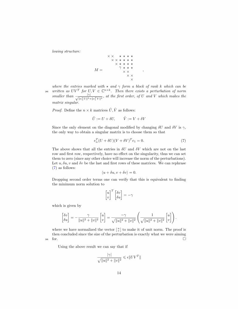
lowing structure:

M =

×××

××? ? ? ?? ? ? ?? ? ? ?? ? ?γ×××

××

,

where the entries marked with ? and γ form a block of rank k which can bewritten as UV T for U, V ∈ Cn×k. Then there exists a perturbation of norm290

smaller than |γ|√‖eTnU‖2+‖eT1 V ‖2

, at the first order, of U and V which makes the

matrix singular.

Proof. Define the n× k matrices U , V as follows:

U := U + δU, V := V + δV

Since the only element on the diagonal modified by changing δU and δV is γ,the only way to obtain a singular matrix is to choose them so that

eTn (U + δU)(V + δV )T e1 = 0. (7)

The above shows that all the entries in δU and δV which are not on the lastrow and first row, respectively, have no effect on the singularity, thus we can setthem to zero (since any other choice will increase the norm of the perturbations).Let u, δu, v and δv be the last and first rows of these matrices. We can rephrase(7) as follows:

〈u+ δu, v + δv〉 = 0.

Dropping second order terms one can verify that this is equivalent to findingthe minimum norm solution to [

uv

]T [δvδu

]= −γ

which is given by[δvδu

]= − γ

‖u‖2 + ‖v‖2

[uv

]=

−γ√‖u‖2 + ‖v‖2

(1√

‖u‖2 + ‖v‖2

[uv

]).

where we have normalized the vector [ uv ] to make it of unit norm. The proof isthen concluded since the size of the perturbation is exactly what we were aimingfor.295

Using the above result we can say that if

|γ|√‖u‖2 + ‖v‖2

6 ε‖UV T ‖

14

then a structured perturbation which is relatively smaller than ε can make theevaluated pencil singular. We will see in Section 4.3 that the matrix can betaken in this upper triangular form by means of Givens rotations. This is usedto compute Newton’s correction, so then we can easily check when we havereached convergence by testing whether |γ| 6 Ku‖UV T ‖

√‖eTnU‖2 + ‖eT1 V ‖2,300

where K is a small constant, depending also on the norm of U and V , and u theunit round-off. Since all these quantities are available during the computation ofNewton’s correction this condition can be checked almost for free, and providesan effective stopping criterion.

4. Efficient computation of Newton’s correction305

In this section we show how the previous results can be turned into a practicalalgorithm. The main issue is the efficient evaluation of Newton’s correction at apoint, which corresponds to computing the trace of the matrix (A−λB)−1B. Inthis section we present a strategy that works both for the Newton and Lagrangelinearizations, with some specific results that only cover the Newton case.310

4.1. Transformation into Hessenberg structure

As we have seen in Section 2.1 and 2.2, the linearizations that we are inter-ested in have the following form:

L(λ) =

[R LT1 (λ)

L2(λ) 0

](8)

with Lj(λ), j = 1, 2 being rectangular kj × (kj + 1) and upper bidiagonal and Rbeing a rank 2 matrix. Without loss of generality, in the following we assumethat L1(λ) and L2(λ) have the same size k × (k + 1) and R = UV T withU, V ∈ C(k+1)×2.315

Theorem 4.1. Let L(λ) be a pencil as in (8). Then there exists a block columnpermutation that takes it to upper Hessenberg form. More precisely, we havethat

L(λ)Π =

[LT1 (λ) R

0 L2(λ)

]=: A− λB, Π =

[Ik+1

Ik

]is an upper Hessenberg pencil. Moreover, its leading coefficient is lower bidi-agonal with a zero element on the diagonal in position (k + 1, k + 1), and theconstant coefficient is the sum of a bidiagonal matrix with an upper triangularrank 2 matrix.

Proof. Direct consequence of applying Π to the pencils defined in Sections 2.1320

and 2.2.

Something more can be said in the Newton case, where the leading coefficientis diagonal. Using an additional permutation, the pencil L(λ) can be endowedwith an Hessenberg-Triangular structure. This is relevant if one wants to applythe QZ iteration, since the reduction to upper Hessenberg-Triangular form is325

15

the usual preliminary step in this case. While this is not directly relevant for theEA approach, it is still a reduction that is interesting so we state the followingresult.

Lemma 4.2. Let L(λ) the pencil obtained by linearizing the sum (or differ-ence) of two polynomials expressed in the Newton basis. Then there exist twopermutation matrices Π1 and Π2 such that

Π1L(λ)Π2 = A− λB,

with B diagonal and A upper Hessenberg.

Proof. We already know, thanks to Theorem 4.1, that we can choose Π2,1 sothat the pencil L(λ)Π2,1 is upper Hessenberg. Let Jk, Π1,1 and Π1,2 be definedas follows:

Jk =

1

. ..

1

, Π1,1 = Jk1+1 ⊕ Ik2 , Π1,2 = Jk1 ⊕ Ik2+1.

Multiplying L(λ)Π2,1 on the left by Π1,1 acts on the first block row as the leftmultiplication by Jk1+1 and, analogously, the right multiplication by Π1,2 actson the right as Jk1 . These transformations preserve the rank of the top-rightblock and leave L2(λ) unchanged. Moreover, in the Newton case, L1(λ)T isgiven by

L1(λ)T = H − λ[0Tk1Ik1

]where H is lower bidiagonal. It can be checked easily that Jk1+1HJk1 is stilllower bidiagonal and that

Jk1+1L1(λ)T Jk1 = Jk1+1HJk1 − λ[Ik10Tk1

]has the prescribed Hessenberg triangular structure when embedded in the larger330

pencil. Setting Π1 := Π1,1 and Π2 := Π2,1Π1,2 completes the proof.

4.2. A Sherman-Morrison based approach

In this section we focus on providing a method involving O(n) flops forcomputing the trace of (A − λB)−1B, i.e., for the evaluation of the Newtoncorrection of the polynomial detL(λ). The method is based on the Sherman-335

Morrison formula [14].

Theorem 4.3 (Sherman-Morrison). Let M and M + UV T be two invertiblematrices, where M ∈ Cn×n and U, V ∈ Cn×k. Then

(M + UV T )−1 = M−1 −M−1U(I + V TM−1U)−1V TM−1.

16

The above formula provides a cheap method to evaluate the inverse of a lowrank correction of a matrix whose inverse is known (or easily computable). Thisis exactly our case, since the pencil L(λ) can be written in the following form:

A− λB = M(λ) + UV T

where M(λ) is a lower bidiagonal pencil and U, V ∈ Cn×2. Unfortunately, theabove decomposition does not satisfy the hypotheses of Theorem 4.3, since thebidiagonal matrix M(λ) has a zero diagonal entry (see Theorem 4.1) and is notinvertible.340

However, we can rephrase the decomposition by modifying M(λ) and puttinga value α 6= 0 in position (k + 1, k + 1) and accordingly modify the rank 2correction to a rank 3 one so that

A− λB = M(λ) + UV T − αek+1eTk+1 = M(λ) + U V T .

In the above formulation the matrix M(λ) is invertible and by the Sherman-Morrison formula we obtain:

(A− λB)−1 = M(λ)−1 − M(λ)−1U(I + V T M(λ)−1U)−1V T M(λ)−1, (9)

which in turn leads to the following result.

Lemma 4.4. Let A−λB be a pencil defined as in Theorem 4.1. Then, for anyλ such that A− λB is invertible and for any α 6= 0,

tr((A− λB)−1B) = tr(M(λ)−1B)− tr(V T (λ)U(λ))

where M(λ), U(λ), V (λ) are defined as in (9) and

U(λ) := M(λ)−1U(I + V T M(λ)−1U)−1, V (λ) = BT M(λ)−T V .

Proof. We can use the decomposition of (9) to get:

(A− λB)−1B = M(λ)−1B − M(λ)−1U(I + V T M(λ)−1U)−1V T M(λ)−1B.

Since the trace is a linear operator, we can split the trace of this sum as the sumof the traces, and using the fact that the trace of a matrix product is invariantunder cyclic permutation of the factors we get the thesis.

The trace of a matrix product can be characterized as follows.345

Lemma 4.5. Let M,N be two n× k matrices. Then

tr(MNT ) =∑

06i,j6n

(M ◦N)ij

where ◦ denotes the Hadamard product.

17

Remark 4.6. We emphasize that Lemma 4.4 provides an O(n) algorithm forcomputing Newton’s correction. In fact, to evaluate the first term of the sumwe can use the relation given by Lemma 4.5:

tr(M(λ)−1B) =∑i,j

(M(λ)−1 ◦BT )ij .

Since BT has only nonzero elements on the diagonal and on the superdiagonalwe have to compute the diagonal and superdiagonal of M(λ)−1, which can bedone in O(n) flops given its bidiagonal structure.

Moreover, the second matrix of which we have to compute the trace is 3× 3350

and can be computed in O(n) flops. These two facts together provide an O(n)algorithm.

Whilst the above framework is theoretically satisfying, from a numericalperspective there are still some points that need to be handled carefully. Anatural one is the choice of α. While any α 6= 0 provides a mathematically355

correct formula, we are interested in choosing α in order to obtain the bestpossible numerical results. In practice we can choose α to be about the normof the other diagonal elements, in order to avoid unbalancing in the matrix.

4.3. Using rotations

As we will see in Section 5 the algorithm of Section 4.2 can be unstable. For360

this reason, it is of interest to devise an alternative scheme based on unitarytransformations that, as confirmed by numerical experiments in Section 5, ismore robust in practice.

In view of Lemma 4.2 we know that, up to permutations, we can rewrite thepencil as A− λB where A and B have the following structure:

A =

[BTφ UV T

0 Bψ

], B =

[−BTφ,1

−Bψ,1

],

where Bφ and Bψ are (rectangular) bidiagonal matrices containing the inter-polation nodes. The Newton case is particularly easy to deal with, since the365

matrix B is diagonal, with a zero entry in the middle. We have the following.

Lemma 4.7. Let A − λB a linearization for a sum of two scalar polynomialsexpressed in two Newton bases as in (3). Then the trace of the matrix (A −λB)−1B can be expressed as follows:

tr((A− λB)−1B

)=

n∑i=1i 6=k+1

[A− λB]−1ii

−1

where k is the degree of the polynomials whose sum is linearized.

Proof. It follows by recalling that tr(ABT ) =∑i,j(A ◦ B)ij , where ◦ is the

Hadamard product of the matrices A and B, see Lemma 4.5.

18

An analogous result (which we do not state explicitly) also holds for the370

Lagrange case, where the linear combination of the diagonal and superdiagonalelements has to be done using the barycentric weights as coefficients.

In both cases, to ease the computation, we will split the inverse of A−λB intwo parts. The linearity of the trace operator allows to compute these two partsseparately and then sum the results. More precisely, we look for a decomposition375

(A−λB)−1 = M1 +M2, so that we can compute tr((A−λB−1)B) = tr(M1B)+tr(M2B). We rely on the following elementary result.

Lemma 4.8. Let X be an upper bidiagonal matrix, defined as follows:

X =

α1 β1

. . .. . .

. . . βn−1

αn

.Then it admits a factorization as a sequence of n − 1 Gauss transformationsgiven by X = Xn−1 . . . X1 where

X1 =

α1 β1

α2

In−2

and Xi =

Ii−1

1 βiαi+1

In−i−1

for i > 1.

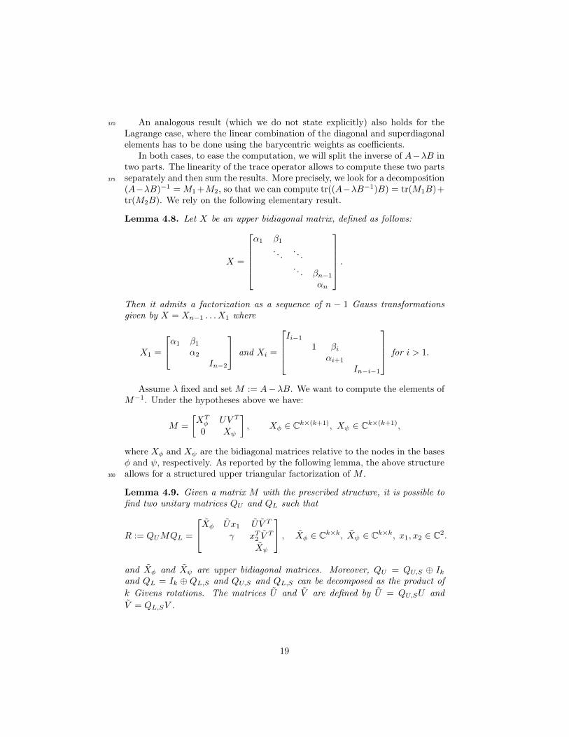
Assume λ fixed and set M := A−λB. We want to compute the elements ofM−1. Under the hypotheses above we have:

M =

[XTφ UV T

0 Xψ

], Xφ ∈ Ck×(k+1), Xψ ∈ Ck×(k+1),

where Xφ and Xψ are the bidiagonal matrices relative to the nodes in the basesφ and ψ, respectively. As reported by the following lemma, the above structureallows for a structured upper triangular factorization of M .380

Lemma 4.9. Given a matrix M with the prescribed structure, it is possible tofind two unitary matrices QU and QL such that

R := QUMQL =

Xφ Ux1 U V T

γ xT2 VT

Xψ

, Xφ ∈ Ck×k, Xψ ∈ Ck×k, x1, x2 ∈ C2.

and Xφ and Xψ are upper bidiagonal matrices. Moreover, QU = QU,S ⊕ Ikand QL = Ik ⊕ QL,S and QU,S and QL,S can be decomposed as the product of

k Givens rotations. The matrices U and V are defined by U = QU,SU and

V = QL,SV .

19

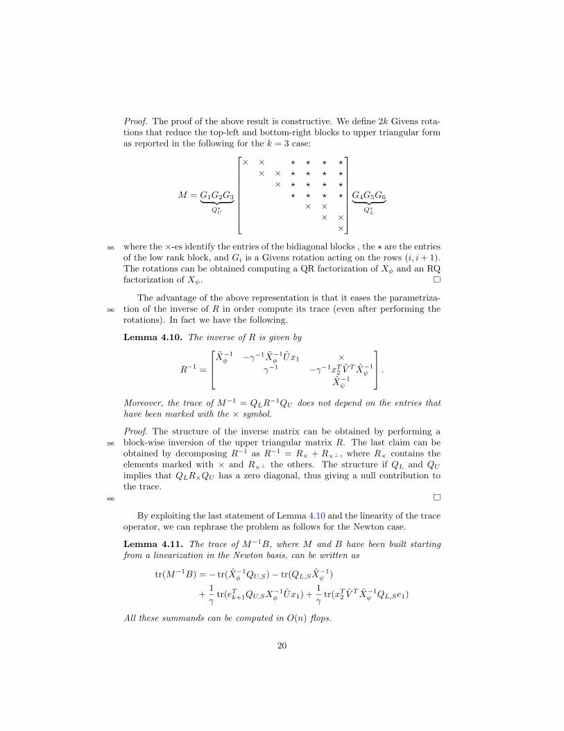
Proof. The proof of the above result is constructive. We define 2k Givens rota-tions that reduce the top-left and bottom-right blocks to upper triangular formas reported in the following for the k = 3 case:

M = G1G2G3︸ ︷︷ ︸Q∗U

× × ? ? ? ?× × ? ? ? ?× ? ? ? ?

? ? ? ?× ×× ××

G4G5G6︸ ︷︷ ︸

Q∗L

where the ×-es identify the entries of the bidiagonal blocks , the ? are the entries385

of the low rank block, and Gi is a Givens rotation acting on the rows (i, i+ 1).The rotations can be obtained computing a QR factorization of Xφ and an RQfactorization of Xψ.

The advantage of the above representation is that it eases the parametriza-tion of the inverse of R in order compute its trace (even after performing the390

rotations). In fact we have the following.

Lemma 4.10. The inverse of R is given by

R−1 =

X−1φ −γ−1X−1

φ Ux1 ×γ−1 −γ−1xT2 V

T X−1ψ

X−1ψ

.Moreover, the trace of M−1 = QLR

−1QU does not depend on the entries thathave been marked with the × symbol.

Proof. The structure of the inverse matrix can be obtained by performing ablock-wise inversion of the upper triangular matrix R. The last claim can be395

obtained by decomposing R−1 as R−1 = R× + R×⊥ , where R× contains theelements marked with × and R×⊥ the others. The structure if QL and QUimplies that QLR×QU has a zero diagonal, thus giving a null contribution tothe trace.

400

By exploiting the last statement of Lemma 4.10 and the linearity of the traceoperator, we can rephrase the problem as follows for the Newton case.

Lemma 4.11. The trace of M−1B, where M and B have been built startingfrom a linearization in the Newton basis, can be written as

tr(M−1B) = − tr(X−1φ QU,S)− tr(QL,SX

−1ψ )

+1

γtr(eTk+1QU,SX

−1φ Ux1) +

1

γtr(xT2 V

T X−1ψ QL,Se1)

All these summands can be computed in O(n) flops.

20

The above results allow to devise an O(n) method to evaluate the Newtoncorrection of detL(λ) at any point in the complex plane.405

Remark 4.12. The computation of the QL, QU and the inversion of the uppertriangular matrix, can be all performed by means of backward stable operations.Moreover, given the structure of A − λB, all the errors are offloaded either onthe nodes or on the low rank part which contains the coefficients of the poly-nomials. This suggests that the procedure for the computation of Newton’s410

correction is structurally backward stable, with respect to the bidiagonal pluslow rank structure. In fact, the final result is the exact one obtained by slightperturbations on the nodes and on the coefficients. As we will see in the numer-ical experiments, this leads to a better accuracy with respect to non-structuredbackward stable methods, like the QZ algorithm.415

5. Numerical experiments

In this section we report the numerical experiments that validate our ap-proach. We have tested two different aspects of the algorithm: the accuracyand the asymptotic cost.

Regarding the former, we verified that in many common cases EAI delivers420

very accurate results. Moreover, we show that it easily overcomes the problemsrelated to poor conditioning of the eigenvalues when considering the unstruc-tured condition number of the eigenvalue problem.

5.1. Accuracy of the method

We consider the problem of finding the roots of a polynomial r(λ) described425

as r(λ) = p1(λ)−p2(λ), with p1(λ) and p2(λ) expressed in the Newton basis. Asnodes for these two interpolation polynomials we have chosen the Chebyshevpoints, in order to have a set of points where the interpolation is reasonablyconditioned. We have computed 2k nodes and we have used k of them togenerate the basis for p1(λ) and k of them to build the basis for p2(λ), so430

they are expressed in a different basis. We have ordered the set of 2k nodesaccording to the canonical ordering on R and we have assigned the ones in theodd positions to the first interpolation basis, and the ones in the even positionto the other, as depicted in Figure 2. The same kind of splitting has been usedfor the roots of unity, which have been employed for the numerical experiments435

in the Lagrange case reported in Table 3 (in this case they have been orderedby their angle).

In Table 1 we have reported the absolute forward errors5 and the back-ward errors (on the matrix pencil) for the approximation of the roots using theSherman-Morrison based strategy and the one based on Givens rotations. More440

precisely, we have computed the backward error err(A,B)(λ) for each eigenvalue

5Approximations for the roots with an arbitrary number of digits have been obtainedusing MPSolve [7], a multiprecision polynomial solver. The symbolic toolbox of MATLAB tocompute the coefficients of the linearized polynomial.

21

−1 1

Figure 2: On the left, the splitting used to assign the 2k Chebyshev nodes to the first andsecond family of nodes, used for p1(λ) and p2(λ), respectively, is reported. On the right, thesame splitting for the roots of unity is shown.

defined as err(A,B)(λ) := σn(A−λB), where σn(·) is the smallest singular value.This can be proven to be the distance (in the Euclidean norm) to the closestpencil that has λ as an eigenvalue. We refer to the work of Tisseur [18] for adetailed error analysis.445

It is clearly visible that the strategy based on rotations does not have stabilityissues, while the accuracy of the one based on Sherman-Morrison soon degradesas the degree increases. For this reason, in the following we will always considerthe strategy based on rotations. The numbers reported are the norms of thevectors containing the errors for each approximation. For the examples that we450

have chosen there is not much difference between absolute and relative errorssince most of the roots have modulus about 1.

Degree Forward SM Forward Rot Backward SM Backward Rot

2 2.14 · 10−16 1.87 · 10−16 6.11 · 10−17 5.18 · 10−17

5 2.06 · 10−15 1.38 · 10−16 4.54 · 10−16 6.76 · 10−17

10 1.83 · 10−13 1.58 · 10−16 1.05 · 10−14 5.66 · 10−17

15 5.68 · 10−11 1.23 · 10−16 9.3 · 10−12 3.69 · 10−17

20 4.01 · 10−6 1.17 · 10−16 3.57 · 10−8 4.22 · 10−17

Table 1: Comparison of the accuracies of the two strategies for the computation of New-ton’s correction. The columns marked with SM represents the data relative to the Sherman-Morrison based approach of Section 4.2, while the ones marked with Rot refer to the strategybased on Givens rotations of Section 4.3.

In Table 2 we have reported both absolute forward errors and backwarderrors (on the matrix pencil) for a wider range of degrees, and we have com-pared it with the QZ algorithm. However, the degradation in the quality of455

the approximations given by the QZ iteration is clearly visible. This is due tothe fact that while giving backward stable results, they are backward stablein an unstructured sense, and they are not guaranteed to correspond to smallperturbations in the polynomials. Since the EAI iteration relies on a structured

22

Degree Forward EAI Forward QZ Backward EAI Backward QZ

10 5.1 · 10−16 3.64 · 10−15 1.02 · 10−16 1.43 · 10−16

20 5.2 · 10−16 5.65 · 10−14 1.55 · 10−16 1.94 · 10−16

40 7.96 · 10−16 3.59 · 10−10 2.33 · 10−16 2.66 · 10−16

80 5.93 · 10−16 0.35 3.38 · 10−16 4.35 · 10−16

160 1.41 · 10−15 1.09 4.62 · 10−16 6.71 · 10−16

Table 2: Numerical accuracy of the EAI compared to the QZ iteration. We have generated50 examples of sums of polynomials whose coefficients in the Newton basis are drawn byGaussian distribution coefficients. The nodes of the Newton bases are Chebyshev points. Theinfinite eigenvalues in the QZ methods have been deflated a posteriori — and have alwaysbeen exactly identified by the QZ method. In this cases a posteriori deflation is easy becauseof the special structure that the linearization has for degree-graded bases. This is not the casein general. The accuracies have been averaged over all the experiments. The backward errorreported in the table is the one on the matrix pencil.

Degree Forward EAI Forward QZ Backward EAI Backward QZ

5 7.25 · 10−16 2.15 · 10−15 1.35 · 10−16 2.21 · 10−16

10 5.85 · 10−16 1.68 · 10−15 1.01 · 10−16 2.33 · 10−16

20 1.52 · 10−14 2.69 · 10−14 8.03 · 10−17 2.02 · 10−16

40 1.58 · 10−15 1.22 · 10−14 4.82 · 10−17 8.37 · 10−17

80 6.8 · 10−15 6.78 · 10−14 2.99 · 10−17 4.56 · 10−17

Table 3: Numerical accuracy of the EAI compared to the QZ iteration for sums of rationalfunctions defined by ratios of Lagrange polynomials. The accuracies have been averaged over10 runs, and the nodes have been chosen with interlacing properties as in the Newton exampleof Table 2 from the roots of unity of appropriate degree.

(and backward stable) solver to compute the Newton correction, evaluating a460

slightly perturbed polynomial, it leads to much better results in practice.

5.2. Asymptotic cost of the method

The speed of convergence of the EAI is strictly related to the quality ofthe starting approximations. In Section 3.1 we have discussed possible choicesfor the starting points, and here we study how these relate to the number of465

iterations before the stopping criterion presented in Section 3.2 is met on all thecomponents.

In particular, we are interested in studying the average number of iterationsper eigenvalue. Since an iteration costs O(n) flops, keeping this number boundedby a constant makes the asymptotic cost O(n2).470

More generally, assuming an instance of EAI has an average number ofiterations equal to t > 0, we have a total cost for the algorithm of O(tn2). Ouraim is to choose the starting points that make t as small as possible. The resultsin Figure 3 show that good starting points produce a very slow growth in thenumber of iteration, thus providing a practically quadratic method.475

23

0 20 40 60 80 100 120 140 1600

20

40

60

80

100

Degree

Ave

rage

iter

atio

ns

per

root

Contour integrationPower method

Figure 3: Average number of iterations for different choices of starting points. The tests referto the computation of the roots of the sum of two polynomial expressed in the Newton basiswith interlaced Chebyshev nodes as described in Figure 2.

Degree Integration Power method

5 6.42 7.6210 7.02 10.4520 7.5 16.8640 9.16 29.5960 9.82 41.3280 11.79 56.67100 12.28 62.72120 13.29 76.01140 15.6 100.51160 16.38 103.02

Table 4: Average number of iterations with different criterion for the choice of the startingpoints.

24

To estimate the value of t we have run the following procedure:

1. We have randomly generated a sequence of rational functions, for variousdegrees from n = 10 up to n = 160 (here by degree we mean the degree ofthe numerator and the denominator). We have chosen the same kind ofNewton basis for all of them and we have drawn random coefficients from480

a Gaussian distribution N(0, 1).

2. We have run the EAI on these problems. 50 problems with the samedegree have been tested and we have computed the average number ofiterations for each degree.

The results of these tests are reported in Table 4 and in Figure 3. We have485

tested the two methods for the choice of the starting points that have beendiscussed in Section 3.1, that is the adapted power method and the integralapproach to counting the number of eigenvalues inside a closed curve. Bothmethods manage to deliver the starting points in (at most) O(n2) flops, so theydo not significantly contribute to the total complexity of the method. More pre-490

cisely, we have fixed the number of integration points or iterations of the powermethod to be bounded by n, so that we have a guaranteed O(n2) complexityfor the computation of the starting points.

Figure 3 shows how, as we have already stressed, even if the contour inte-gration method still exhibits some growth in the average number of iteration as495

n grows, this effect is very mitigated compared to taking points on a circle oflarge enough radius.

The degraded performance of putting all the initial approximations on acircle with radius equal to the spectral radius of the pencil (ignoring infiniteeigenvalues) can be informally explained by the fact that the approximation500

have to travel a long distance to reach the roots with smaller modulus.

5.3. Eigenvalues of matrix polynomials

To complete the section we show an application to the computation of eigen-values of matrix polynomials and rational functions. More precisely, we considerthe nonlinear eigenvalue problem

R(λ)v = 0, R(λ) := P1(λ)−1Q1(λ) + P2(λ)Q2(λ)−1,

where as usual the matrix polynomials P1(λ) and Q1(λ) are expressed in acertain basis, and P2(λ) and Q2(λ) in another one. In this case we assume thatthey are both Newton bases, with different nodes.505

The same approach of Section 4.3 can be used to evaluate the trace of thelinearization of such a nonlinear eigenvalue problem at a certain point in thecomplex plane. Assuming the degree of all the matrix polynomials involved isd one can reduce the diagonal blocks to upper block bidiagonal form with O(d)block Givens rotations, and then compute the inverse of the resulting block510

upper triangular matrix.

25

Degree Forward EAI Forward QZ Backward EAI Backward QZ

2 1.63 · 10−15 1.04 · 10−13 1.02 · 10−18 2.4 · 10−18

4 6.94 · 10−15 1.37 · 10−13 1.11 · 10−18 1.93 · 10−18

6 2.21 · 10−15 2.05 · 10−13 7.77 · 10−19 1.61 · 10−18

8 1.62 · 10−15 3.26 · 10−13 5.77 · 10−19 1.2 · 10−18

10 9.39 · 10−16 2.57 · 10−13 7.1 · 10−19 1.05 · 10−18

12 5.2 · 10−16 3.43 · 10−13 4.98 · 10−19 7.79 · 10−19

14 1.06 · 10−15 3.29 · 10−13 5.16 · 10−19 8.17 · 10−19

16 3.79 · 10−15 5.07 · 10−13 5.45 · 10−19 9.03 · 10−19

18 8.42 · 10−15 7.12 · 10−13 7.09 · 10−19 2.19 · 10−18

20 1.77 · 10−15 8.62 · 10−13 4.51 · 10−19 8.61 · 10−19

22 8.02 · 10−16 1.88 · 10−12 4.34 · 10−19 6.06 · 10−19

24 3.28 · 10−15 7.23 · 10−12 4.96 · 10−19 6.76 · 10−19

Table 5: Numerical accuracy of the EAI compared to the QZ algorithm in the computation ofthe eigenvalues of a nonlinear eigenvalue problem expressed as a sum of two rational functionsin the Newton basis. The nodes of the Newton bases are Chebyshev points.

The cost of each evaluation of Newton’s correction is cubic in the size of thecoefficients, leading to a total computational cost of O((dn) · dn3) = O(dn4),so this approach is convenient only if the degree is large enough. We havecompared the results obtained using the EA iteration to the QZ on the pencil,515

and also in this case one notices that the (forward) accuracy of the EA is muchbetter than the one of the QZ. However, both algorithms deliver backward stableapproximations, as reported in Table 5.

The coefficients of the matrix polynomials in this example are random 6× 6matrices with integer entries between −1000 and 1000. This setup has been520

chosen to allow the computation of the eigenvalues symbolically in order tocheck the computed results. The backward error computed (which is relative tothe norms of the pencil) is always below the machine precision, and the resultsof the QZ algorithm show that the (unstructured) eigenvalue condition numberof the pencil is still quite high compared to the structured one (that is, the one525

of the original problem).

6. Conclusions

We have shown the effectiveness of the Ehrlich–Aberth iteration as an ap-proximation engine for the eigenvalues of some rank structured pencils whichare encountered when linearizing sums of polynomials and rational functions530

expressed in Newton Lagrange bases. Our approach allows to treat a broad setof problems, such as (matrix) polynomials and rational functions expressed assums in different bases.

This work has shown that the method is both fast, in the sense of havinga lower asymptotic complexity than the QR and the QZ iterations, and more535

26

accurate when looking at the forward errors. The gain is obtained by applyinga structured solver that only allows perturbations on the original input data.Moreover, we have shown that the deflation of infinite eigenvalue is not anissue in this context, simplifying the analysis. Thus, even when some of theeigenvalues are ill-conditioned in the pencil no loss of accuracy is encountered540

with the EAI.We have derived suitable strategies and methods for the estimation of the

starting points which have shown to be effective in practice, and we have deviseda practical criterion for the stopping conditions.

We think this proves both the flexibility of the EAI, which has been adapted545

to this case with the development of proper tools, and the importance of consid-ering structured iterations for the approximation of eigenvalues of linearizations.This is particularly interesting for applications where the data is naturally ex-pressed in different bases (or the same bases with different nodes), such as thetransfer functions for closed loop linear systems [16], or the clipping problems550

in computer aided graphics [12].

References

[1] Aberth, O., 1973. Iteration methods for finding all zeros of a polynomialsimultaneously. Mathematics of computation 27 (122), 339–344.

[2] Ball, J. A., Gohberg, I., et al., 2013. Interpolation of rational matrix func-555

tions. Vol. 45. Birkhauser.

[3] Berrut, J.-P., Trefethen, L. N., 2004. Barycentric Lagrange interpolation.SIAM Review 46 (3), 501–517.

[4] Bini, D. A., Gemignani, L., Tisseur, F., 2005. The Ehrlich–Aberth Methodfor the Nonsymmetric Tridiagonal Eigenvalue Problem. SIAM Journal on560

Matrix Analysis and Applications 27 (1), 153–175.

[5] Bini, D. A., Meini, B., 2015. Generalization of the Brauer Theo-rem to Matrix Polynomials and Matrix Laurent Series. arXiv preprintarXiv:1512.07118.

[6] Bini, D. A., Noferini, V., 2013. Solving polynomial eigenvalue problems by565

means of the Ehrlich–Aberth method. Linear Algebra and its Applications439 (4), 1130–1149.

[7] Bini, D. A., Robol, L., 2014. Solving secular and polynomial equations: Amultiprecision algorithm. Journal of Computational and Applied Mathe-matics 272, 276292.570

[8] Brauer, A., 1946. Limits for the characteristic roots of a matrix. DukeMathematical Journal 13 (3), 387–395.

[9] Datta, B. N., 2010. Numerical Linear Algebra and Applications. SIAM.

27

[10] Edelman, A., Murakami, H., 1995. Polynomial roots from companion ma-trix eigenvalues. Mathematics of Computation 64 (210), 763–776.575

[11] Ehrlich, L. W., 1967. A modified Newton method for polynomials. Com-munications of the ACM 10 (2), 107–108.

[12] Farin, G., 2014. Curves and surfaces for computer-aided geometric design:a practical guide. Elsevier.

[13] Forney Jr, G. D., 1975. Minimal bases of rational vector spaces, with ap-580

plications to multivariable linear systems. SIAM Journal on Control 13 (3),493–520.

[14] Gustafson, W. H., 1984. A note on matrix inversion. Linear algebra and itsapplications 57, 71–73.

[15] Henrici, P., 1974. Computational complex analysis. In: Proceedings Sym-585

posium Applied Mathematics. Vol. 20. pp. 79–86.

[16] Kailath, T., 1980. Linear systems. Vol. 156. Prentice-Hall Englewood Cliffs,NJ.

[17] Robol, L., Vandebril, R., Dooren, P. V., 2017. A framework for structuredlinearizations of matrix polynomials in various bases. SIAM Journal on590

Matrix Analysis and Applications 38 (1), 188–216.

[18] Tisseur, F., 2000. Backward error and condition of polynomial eigenvalueproblems. Linear Algebra and its Applications 309 (1), 339–361.

[19] Trefethen, L. N., Weideman, J., 2014. The exponentially convergent trape-zoidal rule. SIAM Review 56 (3), 385–458.595

[20] Van Beeumen, R., Michiels, W., Meerbergen, K., 2015. Linearization ofLagrange and Hermite interpolating matrix polynomials. IMA Journal ofNumerical Analysis 35 (2), 909–930.

[21] Walsh, J. L., 1935. Interpolation and approximation by rational functionsin the complex domain. Vol. 20. American Mathematical Soc.600

[22] Whittaker, S. E., Robinson, G., 1924. The Calculus of Observations. BlackieAnd Son Limited.

28