e a - University of Cambridge · (Unless we think humans ... Why people think computers can't,...
89
Artificial Intelligence I Dr Sean Holden Computer Laboratory, Room FC06 Telephone extension 63725 Email: [email protected] www.cl.cam.ac.uk/∼sbh11/ Copyright c Sean Holden 2002-2012. 1 Introduction: what’s AI for? What is the purpose of Artificial Intelligence (AI)? If you’re a philosopher or a psychologist then perhaps it’s: • To understand intelligence. • To understand ourselves. Philosophers have worked on this for at least 2000 years. They’ve also wondered about: • Can we do AI? Should we do AI? • Is AI impossible? (Note: I didn’t write possible here, for a good reason...) Despite 2000 years of work, there’s essentially diddly-squat in the way of results. 2 Introduction: what’s AI for? Luckily, we were sensible enough not to pursue degrees in philosophy—we’re scientists/engineers, so while we might have some interest in such pursuits, our perspective is different: • Brains are small (true) and apparently slow (not quite so clear-cut), but incred- ibly good at some tasks—we want to understand a specific form of computa- tion. • It would be nice to be able to construct intelligent systems. • It is also nice to make and sell cool stuff . This view seems to be the more successful. . . AI is entering our lives almost without us being aware of it. 3 Introduction: now is a fantastic time to investigate AI In many ways this is a young field, having only really got under way in 1956 with the Dartmouth Conference. www-formal.stanford.edu/jmc/history/dartmouth/dartmouth.html • This means we can actually do things. It’s as if we were physicists before anyone thought about atoms, or gravity, or.... • Also, we know what we’re trying to do is possible. (Unless we think humans don’t exist. NOW STEP AWAY FROM THE PHILOSOPHY before SOMEONE GETS HURT!!!!) Perhaps I’m being too hard on them; there was some good groundwork: Socrates wanted an algorithm for “piety”, leading to Syllogisms. Ramon Lull’s concept wheels and other attempts at mechanical calculators. Rene Descartes’ Dualism and the idea of mind as a physical system. Wilhelm Leibnitz’s opposing position of Materialism. (The intermediate position: mind is physical but unknowable.) The origin of knowledge: Francis Bacon’s Empiricism, John Locke: “Nothing is in the understanding, which was not first in the senses”. David Hume: we obtain rules by repeated exposure: Induction. Further developed by Bertrand Russel and in the Confirmation Theory of Carnap and Hempel. More recently: the connection between knowledge and action? How are actions justified? If to achieve the end you need to achieve something intermediate, consider how to achieve that, and so on. This approach was implemented in Newell and Simon’s 1957 General Problem Solver (GPS). 4
Transcript of e a - University of Cambridge · (Unless we think humans ... Why people think computers can't,...

Artificial Intelligence I
Dr Sean Holden
Computer Laboratory, Room FC06
Telephone extension 63725
Email: [email protected]
www.cl.cam.ac.uk/∼sbh11/
Copyright c© Sean Holden 2002-2012.
1
Introduction: what’s AI for?
What is the purpose of Artificial Intelligence (AI)? If you’re aphilosopheror apsychologistthen perhaps it’s:
• To understand intelligence.
• To understandourselves.
Philosophers have worked on this for at least2000 years. They’ve also wonderedabout:
• Canwe do AI?Shouldwe do AI?
• Is AI impossible? (Note: I didn’t writepossiblehere, for a good reason...)
Despite2000 years of work, there’s essentiallydiddly-squatin the way of results.
2
Introduction: what’s AI for?
Luckily, we were sensible enough not to pursue degrees in philosophy—we’rescientists/engineers, so while we might havesomeinterest in such pursuits, ourperspective is different:
• Brains are small (true) and apparently slow (not quite so clear-cut), but incred-ibly good at some tasks—we want to understand a specific form of computa-tion.
• It would be nice to be able toconstructintelligent systems.
• It is also nice tomake and sell cool stuff.
This viewseems to be the more successful. . .
AI is entering our lives almost without us being aware of it.
3
Introduction: now is a fantastic time to investigate AI
In many ways this is a young field, having only really got underway in 1956 withtheDartmouth Conference.
www-formal.stanford.edu/jmc/history/dartmouth/dartmouth.html
• This means we can actuallydo things. It’s as if we were physicists beforeanyone thought about atoms, or gravity, or. . . .
• Also, we know what we’re trying to do ispossible. (Unless we think humansdon’t exist.NOW STEP AWAY FROM THE PHILOSOPHYbeforeSOMEONEGETS HURT!!!!)
Perhaps I’m being too hard on them; there was some good groundwork: Socrateswanted an algorithm for“piety” ,leading toSyllogisms. Ramon Lull’sconcept wheelsand other attempts at mechanical calculators. Rene Descartes’Dualism and the idea of mind as aphysical system. Wilhelm Leibnitz’s opposing position ofMaterialism. (Theintermediate position: mind isphysicalbutunknowable.) The origin ofknowledge: Francis Bacon’sEmpiricism, JohnLocke: “Nothing is in the understanding, which was not first in the senses”. David Hume: we obtain rules by repeatedexposure:Induction. Further developed by Bertrand Russel and in theConfirmation Theoryof Carnap and Hempel.
More recently: the connection betweenknowledgeandaction? How are actionsjustified? If to achieve the end youneed to achieve something intermediate, consider how to achieve that, and so on. This approach was implemented inNewell and Simon’s 1957General Problem Solver (GPS).
4

Is AI possible?
Many philosophers are particularly keen to argue that AI isimpossible? Why isthis? We have:
• Perception (vision, speech processing...)
• Logical reasoning (prolog, expert systems, CYC...)
• Playing games (chess, backgammon, go...)
• Diagnosis of illness (in various contexts...)
• Theorem proving (Robbin’s conjecture...)
• Literature and music (automated writing and composition...)
• And many more...
What’s made the difference? In a nutshell:we’re the first lucky bunch to get ourhands on computers, and that allows us tobuild things.
The simple ability totry things outhas led to huge advances in a relatively shorttime. So: don’t believe the critics...
5
Further reading
Why do people dislike the idea that humanity might not bespecial.
An excellent article on why this view is much more problematic than it mightseem is:
“Why people think computers can’t,”Marvin Minsky. AI Magazine, volume 3number 4, 1982.
6
Aside: when something is understood it stops being AI
To have AI, you need a means ofimplementingthe intelligence. Computers are (atpresent) the only devices in the race. (Althoughquantum computationis lookinginteresting...)
AI has had a major effect on computer science:
• Time sharing
• Interactive interpreters
• Linked lists
• Storage management
• Some fundamental ideas in object-oriented programming
• and so on...
When AI has a success, the ideas in question tend tostop being called AI.
Similarly: do you consider the fact thatyour phone can do speech recognitiontobe a form of AI?
7
The nature of the pursuit
What is AI?This is not necessarily a straightforward question.
It depends on who you ask...
We can find many definitions and a rough categorisation can be made dependingon whether we are interested in:
• The way in which a systemactsor the way in which itthinks.
• Whether we want it to do this in ahumanway or arational way.
Here, the wordrational has a special meaning: it meansdoing the correct thingin given circumstances.
8

Acting like a human
What is AI, version one: acting like a human
Alan Turingproposed what is now known as theTuring Test.
• A human judge is allowed to interact with an AI program via a terminal.
• This is theonly method of interaction.
• If the judge can’t decide whether the interaction is produced by a machine oranother human then the program passes the test.
In theunrestrictedTuring test the AI program may also have a camera attached,so that objects can be shown to it, and so on.
9
Acting like a human
The Turing test is informative, and (very!) hard to pass.
• It requires many abilities that seem necessary for AI, such as learning.BUT:a human child would probably not pass the test.
• Sometimes an AI system needs human-like acting abilities—for exampleex-pert systemsoften have to produce explanations—butnot always.
See theLoebner Prize in Artificial Intelligence:
www.loebner.net/Prizef/loebner-prize.html
10
Thinking like a human
What is AI, version two: thinking like a human
There is always the possibility that a machineacting like a human does not actu-ally think. Thecognitive modellingapproach to AI has tried to:
• Deducehow humans think—for example byintrospectionor psychologicalexperiments.
• Copy the process by mimicking it within a program.
An early example of this approach is theGeneral Problem Solverproduced byNewell and Simon in 1957. They were concerned with whether ornot the programreasoned in the same manner that a human did.
Computer Science+ Psychology= Cognitive Science
11
Thinking rationally: the “laws of thought”
What is AI, version three: thinking rationally
The idea that intelligence reduces torational thinkingis a very old one, going atleast as far back as Aristotle as we’ve already seen.
The general field oflogic made major progress in the 19th and 20th centuries,allowing it to be applied to AI.
• We canrepresentandreasonabout many different things.
• The logicist approach to AI.
This is a very appealing idea.However...
12

Thinking rationally: the “laws of thought”
Unfortunately there are obstacles to any naive applicationof logic. It is hard to:
• Representcommonsense knowledge.
• Deal withuncertainty.
• Reason without being tripped up bycomputational complexity.
These will be recurring themes in this course, and in AI II.
Logic alone also falls short because:
• Sometimes it’s necessary to act when there’sno logical course of action.
• Sometimes inference isunnecessary(reflex actions).
13
Further reading
The Fifth Generation Computer Systemproject has most certainly earned thebadge of“heroic failure” .
It is an example of how much harder the logicist approach is than you might think:
“Overview of the Fifth Generation Computer Project,”Tohru Moto-oka. ACMSIGARCH Computer Architecture News, volume 11, number 3, 1983.
14
Acting rationally
What is AI, version four: acting rationally
Basing AI on the idea ofacting rationallymeans attempting to design systemsthat act toachieve their goalsgiven theirbeliefs.
Thinking about this in engineering terms, it seemsalmost inevitablyto lead ustowards the usual subfields of AI. What might be needed?
• To makegood decisionsin manydifferent situationswe need torepresentandreasonwith knowledge.
• We need to deal withnatural language.
• We need to be able toplan.
• We needvision.
• We needlearning.
And so on, so all the usual AI bases seem to be covered.
15
Acting rationally
The idea ofacting rationallyhas several advantages:
• The concepts ofaction, goal andbelief can be defined precisely making thefield suitable for scientific study.
This is important: if we try to model AI systems on humans, we can’t even proposeanysensible definition ofwhat a belief or goal is.
In addition, humans are a system that is still changing and adapted to a very spe-cific environment.
Rational actingdoes not have these limitations.
16
Acting rationally
Rational actingalso seems toincludetwo of the alternative approaches:
• All of the things needed to pass a Turing test seem necessary for rational act-ing, so this seems preferable to theacting like a humanapproach.
• The logicist approach can clearly formpart of what’s required to act rationally,so this seems preferable to thethinking rationallyapproach alone.
As a result, we will focus on the idea of designing systems that act rationally.
17
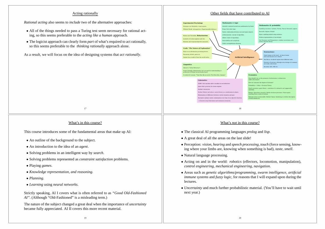
Other fields that have contributed to AI
Artificial Intelligence
Experimental Psychology
Hermann von Helmholtz: visual system.
Wilhelm Wundt: introspection. (Experimentally dubious.)
Watson and Thorndike: Behaviourism
Learned a lot about pigeons and rats.
Stimulus and response/objective measures.
Craik: "The Nature of Explanation"
Brain as an information processing device.
Reasoning, beliefs, goals etc.
System has a model of how the world works.
Mathematics I: logic
Aristotle's material turned into mathematics by Boole
Frege: first order logic.
Tarski: relationship between real and logical objects.
al-Khowarazmi: concept of algorithm.
Hilbert: limits of algorithms.
Intractability and complexity.
Godel: incompleteness theorem.
Mathematics II: probability
Gambling outcomes: Cardano, Fermat, Pascal, Bernoulli, Laplace.
Bernoulli: degree of belief.
Bayes: updating beliefs using evidence.
Modern representation of uncertainty.
Von Neumann and Morgenstern: combine uncertainty with
action: decision theory.
Linguistics
Skinner's "Verbal Behaviour".
Noam Chomsky: behaviourisn can't account for understanding or
production of things not previously heard.
A central AI concept: "Time flies like an arrow. Fruit flies like a banana". Economics
How should I act, in the presence of adversaries, to obtain nice
stuff in the future?
How do I measure the degree of niceness?
Probability + Utility = Decision Theory.
Small economies: game theory - sometimes it's rational to act (apparently)
randomly.
Belman: Operations research. Markov decision processes. Future gains
resulting from a series of actions.
Rational action is intractable. Herbert Simon: Satisficing is a better description
of what humans do.
Neuroscience
Nasty bumps on the head - we know brains
and consciousness are related.
Paul Broca: localised regions have different tasks.
Presence of neurons, although even storage of a memory
not really understood.
Recently: EEG, MRI etc.
Cybernetics
250BC: first machine able to modify its own behaviour.
James Watt: governor for steam engines.
Drebbel: thermostat.
Norbert Weiner and others: control theory as a mathematical subject.
Minimisation of difference between current situation and goal.
Stochastic optimal control: minimisation over time of an objective function.
----AI moves away from linear and continuous scenarios.
18
What’s in this course?
This course introduces some of the fundamental areas that make up AI:
• An outline of the background to the subject.
• An introduction to the idea of anagent.
• Solving problems in an intelligent way bysearch.
• Solving problems represented asconstraint satisfactionproblems.
• Playinggames.
• Knowledge representation, and reasoning.
• Planning.
• Learningusingneural networks.
Strictly speaking, AI I covers what is often referred to as“Good Old-FashionedAI” . (Although “Old-Fashioned” is a misleading term.)
The nature of the subject changed a great deal when the importance ofuncertaintybecame fully appreciated. AI II covers this more recent material.
19
What’snot in this course?
• The classical AI programming languagesprolog andlisp.
• A great deal of all the areas on the last slide!
• Perception:vision, hearingandspeech processing, touch(force sensing, know-ing where your limbs are, knowing when something is bad),taste, smell.
• Natural language processing.
• Acting on and in the world:robotics (effectors, locomotion, manipulation),control engineering, mechanical engineering, navigation.
• Areas such asgenetic algorithms/programming, swarm intelligence, artificialimmune systemsandfuzzy logic, for reasons that I will expand upon during thelectures.
• Uncertaintyand much further probabilistic material. (You’ll have to wait untilnext year.)
20

Text book
The course is based on the relevant parts of:
Artificial Intelligence: A Modern Approach, Third Edition (2010). Stuart Russelland Peter Norvig, Prentice Hall International Editions.
NOTE:This is also the main recommended text for AI2.
21
Interesting things on the web
A few interesting web starting points:
The Honda Asimo robot:world.honda.com/ASIMO
AI at Nasa Ames:www.nasa.gov/centers/ames/research/exploringtheuniverse/spiffy.html
DARPA Grand Challenge:http://www.darpagrandchallenge.com/
2007 DARPA Urban Challenge:cs.stanford.edu/group/roadrunner
The Cyc project:www.cyc.com
Human-like robots:www.ai.mit.edu/projects/humanoid-robotics-group
Sony robots:support.sony-europe.com/aibo
NEC “PaPeRo”:www.nec.co.jp/products/robot/en
22
Prerequisites
The prerequisites for the course are: first order logic, somealgorithms and datastructures, discrete and continuous mathematics, basic computational complexity.
DIRE WARNING:
In the lectures onmachine learningI will be talking aboutneural networks.
This means you will need to be able todifferentiateand also handlevectors andmatrices.
If you’ve forgotten how to do thisyou WILL get lost—I guarantee it!!!
23
Prerequisites
Self test:
1. Let
f(x1, . . . , xn) =n∑
i=1
aix2i
where theai are constants. Can you compute∂f/∂xj where1 ≤ j ≤ n?
2. Letf(x1, . . . , xn) be a function. Now assumexi = gi(y1, . . . , ym) for eachxiand some collection of functionsgi. Assuming all requirements for differentia-bility and so on are met, can you write down an expression for∂f/∂yj where1 ≤ j ≤ m?
If the answer to either of these questions is “no” then it’s time for some revision.(You have about three weeks notice, so I’ll assume you know it!)
24

And finally. . .
There are some important points to be made regardingcomputational complexity.
First, you might well hear the termAI-completebeing used a lot. What does itmean?
AI-complete: only solvable if you can solve AI in its entirety.
For example: high-quality automatic translation from one language to another.
To produce a genuinely good translation ofMoby Dickfrom English to Cantoneseis likely to be AI complete.
25
And finally. . .
More practically, you will often hear me make the claim thateverything that’s atall interesting in AI is at least NP-complete.
There are two ways to interpret this:
1. The wrong way: “It’s all a waste of time.1” OK, so it’s a partly understandableinterpretation.BUT the fact that the travelling salesman problem is intractabledoes notmean there’s no such thing as a satnav. . .
2. The right way: “It’s an opportunity to design nice approximation algorithms.”In reality, the algorithms that aregood in practiceare ones that try tooftenfindagoodbut not necessarilyoptimalsolution, in areasonableamount of time.
1In essence, a comment on a course assessment a couple of yearsback to the effect of: “Why do you teach us this stuff if it’s all futile?”
26
Artificial Intelligence I
Dr Sean Holden
An introduction toAgents
Copyright c© Sean Holden 2002-2012.
27
Agents
There are many different definitions for the termagentwithin AI.
Allow me to introduceEVIL ROBOT.
ENVIRONMENT
Act
Sense
GLORIOUS LEADER!!!!DR HOLDEN WILL BE OUR
MUST ENSLAVE EARTH!!!
We will use the following simple definition:an agent is any device that can senseand act upon its environment.
28

Agents
This definition can be very widely applied: to humans, robots, pieces of software,and so on.
We are taking quite anappliedperspective. We want tomake thingsrather thancopy humans, so to be scientific there are some issues to be addressed:
• How can we judge an agent’s performance?
• How can an agent’senvironmentaffect its design?
• Are there sensible ways in which to think about thestructureof an agent?
Recall that we are interested in devices thatact rationally, where ‘rational’ meansdoing thecorrect thingundergiven circumstances.
Reading:Russell and Norvig, chapter 2.
29
Measuring performance
How can we judge an agent’s performance? Any measure of performance is likelyto beproblem-specific.
Example:For a chess playing agent, we might use its rating.
Example: For a mail-filtering agent, we might devise a measure of how well itblocks spam, but allows interesting email to be read.
Example:For a car driving agent the measure needs considerable sophistication:we need to take account of comfort, journey time, safetyetc.
So: the choice of a performance measure is itself worthy of careful consideration.
30
Measuring performance
We’re usually interested inexpected, long-term performance.
• Expectedperformance because usually agents are notomniscient—they don’tinfallibly know the outcome of their actions.
• It is rational for you to enter this lecture theatre even if the roof falls intoday.
An agent capable of detecting and protecting itself from a falling roof might bemoresuccessfulthan you, butnot morerational.
• Long-term performancebecause it tends to lead to better approximations towhat we’d consider rational behaviour.
• We probably don’t want our car driving agent to be outstandingly smooth andsafe for most of the time, but have episodes ofdriving through the local or-phanage at 150 mph.
31
Environments
How can an agent’senvironmentaffect its design?Example:the environment fora chess programis vastly different to that for anautonomous deep-space vehi-cle. Some common attributes of an environment have a considerable influence onagent design.
• Accessible/inaccessible:do percepts tell youeverythingyou need to knowabout the world?
• Deterministic/non-deterministic:does the future dependpredictablyon thepresent and your actions?
• Episodic/non-episodicis the agent run in independent episodes.
• Static/dynamic:can the world change while the agent is deciding what to do?
• Discrete/continuous:an environment is discrete if the sets of allowable per-cepts and actions are finite.
32

Environments
All of this assumes there is only one agent.
When multiple agents are involved we need to consider:
• Whether the situation iscompetitiveor cooperative.
• Whethercommunicationrequired?
An example of multiple agents:
news.bbc.co.uk/1/hi/technology/3486335.stm
33
Basic structures for intelligent agents
Are there sensible ways in which to think about thestructureof an agent? Again,this is likely to beproblem-specific, although perhaps to a lesser extent.
So far, an agent is based on percepts, actions and goals.
Example:Aircraft piloting agent.
Percepts:sensor information regarding height, speed, enginesetc, audio and videoinputs, and so on.
Actions:manipulation of the aircraft’s controls.
Also, perhaps talking to the passengersetc.
Goals:get to the necessary destination as quickly as possible withminimal use offuel, without crashingetc.
34
Programming agents
A basic agent can be thought of as working on a straightforward underlying pro-cess:
• Gather perceptions.
• Updateworking memoryto take account of them.
• On the basis of what’s in the working memory,choose an actionto perform.
• Updatethe working memory to take account of this action.
• Do the chosen action.
Obviously, this hides a great deal of complexity.
Also, it ignores subtleties such as the fact that a percept might arrive while anaction is being chosen.
35
Programming agents
We’ll initially look at two hopelessly limited approaches,because they do suggesta couple of important points.
Hopelessly limited approach number 1:use a table to map percept sequences toactions. This can quickly be rejected.
• The table will behugefor any problem of interest. About35100 entries for achess player.
• We don’t usually know how to fill the table.
• Even if we allow table entries to belearnedit will take too long.
• The system would have noautonomy.
We can attempt to overcome these problems by allowing agentsto reason.
Autonomyis an interesting issue though...
36

Autonomy
If an agent’s behaviour depends in some manner on itsown experience of theworld via its percept sequence, we say it isautonomous.
• An agent using only built-in knowledge would seem not to be successful at AIin any meaningful sense: its behaviour is predefined by its designer.
• On the other handsomebuilt-in knowledge seems essential, even to humans.
Not all animals are entirely autonomous.
For example:dung beetles.
37
Reflex agents
Hopelessly limited approach number 2:try extractingpertinent information andusingrulesbased on this.
Condition-action rules:if a certainstateis observedthen perform someaction
Some points immediately present themselves regardingwhyreflex agents are un-satisfactory:
• We can’t always decide what to do based on thecurrent percept.
• However storingall past percepts might be undesirable (for example requiringtoo much memory) or just unnecessary.
• Reflex agents don’t maintain a description of thestate of their environment...
• ...however this seems necessary for any meaningful AI. (Consider automatingthe task of driving.)
This is all the more important as usually percepts don’t tellyou everything aboutthe state.
38
Keeping track of the environment
It seems reasonable that an agent should maintain:
• A description of the current state of its environment.
• Knowledge of how the environmentchanges independently of the agent.
• Knowledge of how the agent’sactions affect its environment.
This requires us to doknowledge representationandreasoning.
39
Goal-based agents
It seems reasonable that an agent should choose a rational course of action de-pending on itsgoal.
• If an agent has knowledge of how its actions affect the environment, then ithas a basis for choosing actions to achieve goals.
• To obtain asequenceof actions we need to be able tosearchand toplan.
This is fundamentally differentfrom a reflex agent.
For example:by changing the goal you can change the entire behaviour.
40

Goal-based agents
We now have a basic design that looks something like this:
Description of Goal
Infer
Update
Percept
Description: current environment
Description: effect of actions
Description: behaviour of environment
Update
Action/Action sequence
41
Utility-based agents
Introducing goals is still not the end of the story.
There may bemanysequences of actions that lead to a given goal, andsome maybe preferable to others.
A utility function maps a state to a number representing the desirability of thatstate.
• We can trade-offconflicting goals, for example speed and safety.
• If an agent has several goals and is not certain of achieving any of them, thenit can trade-off likelihood of reaching a goal against the desirability of gettingthere.
Maximising expected utilityover time forms a fundamental model for the designof agents. However we don’t get as far as that until AI II.
42
Learning agents
It seems reasonable that an agent shouldlearn from experience.
Learner
Description of Goal
Feedback
Infer
Update
Percept
Description: current environment
Description: effect of actions
Description: behaviour of environment
Update
Action/Action sequence
Update
43
Learning agents
This requires two additions:
• The learner needs some form offeedbackon the agent’s performance. Thiscan come in several different forms.
• In general, we also need a means ofgenerating new behaviourin order to findout about the world.
This in turn implies a trade-off: should the agent spend timeexploitingwhat it’slearned so far, orexploringthe environment on the basis that it might learn some-thing really useful?
44

What have we learned? (No pun intended...)
Thecrucial things that should be taken away from this lecture are:
• The nature of an agent depends on itsenvironmentandperformance measure.
• We’re usually interested inexpected, long-term performance.
• Autonomy requires that an agent in some way behavesdepending on its expe-rience of the world.
• There is anatural basic structureon which agent design can be based.
• Consideration of that structure leads naturally to the basic areas covered in thiscourse.
Those basic areas are:knowledge representation and reasoning, search, planningand learning. Oh, and finally, we’ve learned NOT TO MESS WITHEVIL ROBOT... he’s a VERY BAD ROBOT!
45
Artificial Intelligence I
Dr Sean Holden
Notes onproblem solving by search
Copyright c© Sean Holden 2002-2012.
46
Problem solving by search
We begin with what is perhaps the simplest collection of AI techniques: those al-lowing anagentexisting within anenvironmentto searchfor asequence of actionsthatachieves a goal.
The algorithms can, crudely, be divided into two kinds:uninformedandinformed.
Not surprisingly, the latter are more effective and so we’lllook at those in moredetail.
Reading:Russell and Norvig, chapters 3 and 4.
47
Problem solving by search
As with any area of computer science, some degree ofabstractionis necessarywhen designing AI algorithms.
Search algorithmsapply to a particularly simple class of problems—we need toidentify:
• An initial state: what is the agent’s situation to start with?
• A set of actions: these are modelled by specifying what state will result onperforming any available action from any known state.
• A goal test: we can tell whether or not the state we’re in corresponds to agoal.
Note that the goal may be described by a property rather than an explicit state orset of states, for examplecheckmate.
48

Problem solving by search
A simple example:the 8-puzzle.
3 5
1 4 2
7 8 6
3 5
4 2
7 8 6
1
3 5
2
7 8 6
1
4
7 8
4 5 6
2 31
−→
−→
−→ · · · −→
Action
Action
Start State
Goal State
Further actions
(A good way of keeping kids quiet...)
49
Problem solving by search
Start state:a randomly-selected configuration of the numbers1 to 8 arranged ona3× 3 square grid, with one square empty.
Goal state:the numbers in ascending order with the bottom right square empty.
Actions: left, right, up, down. We can move any square adjacent to theempty square into the empty square. (It’s not always possible to choose from allfour actions.)
Path cost:1 per move.
The 8-puzzle is very simple. However general sliding block puzzles are a goodtest case. The general problem is NP-complete. The5× 5 version has about1025
states, and a random instance is in fact quite a challenge.
50
Problem solving by basic search
EVIL ROBOT has found himself in an unfamiliar building:
ODIN
Evil Robot
Teleport
He wants theODIN (Oblivion Device of Indescribable Nastiness).
51
Problem solving by search
Start state:EVIL ROBOT is in the top left corner.
Goal state:EVIL ROBOT is in the area containing the ODIN.
Actions: left, right, up, down. We can move as long as there’s no wall inthe way. (Again, it’s not always possible to choose from all four actions.)
Path cost:1 per move. If you step on a teleport then you move to the other onewith a cost of0.
52

Problem solving by search
Problems of this kind are very simple, but a surprisingly large number of applica-tions have appeared:
• Route-finding/tour-finding.
• Layout of VLSI systems.
• Navigation systems for robots.
• Sequencing for automatic assembly.
• Searching the internet.
• Design of proteins.
and many others...
Problems of this kind continue to form an active research area.
53
Problem solving by search
It’s worth emphasising that a lot of abstraction has taken place here:
• Can the agent know it’s current state in full?
• Can the agent know the outcome of its actions in full?
Single-state problems:the state is always known precisely, as is the effect of anyaction. There is therefore a single outcome state.
Multiple-state problems:The effects of actions are known, but the state can notreliably be inferred, or the state is known but not the effects of the actions.
Both single and multiple state problems can be handled usingthese search tech-niques. In the latter, we must reason about the set of states that we could be in:
• In this case we have an initialsetof states.
• Each action leads to a furthersetof states.
• The goal is a set of statesall of which are valid goals.
54
Problem solving by search
Contingency problems
In some situations it is necessary to perform sensingwhile the actions are beingcarried out in order to guarantee reaching a goal.
(It’s good to keep your eyes open while you cross the road!)
This kind of problem requiresplanningand will be dealt with later.
55
Problem solving by search
Sometimes it is actively beneficial to act and see what happens, rather than to tryto consider all possibilities in advance in order to obtain aperfect plan.
Exploration problems
Sometimes you haveno knowledge of the effect that your actions have on theenvironment.
Babies in particular have this experience.
This means you need to experiment to find out what happens whenyou act.
This kind of problem requiresreinforcement learningfor a solution. We will notcover reinforcement learning in this course. (Although it is in AI II.)
56
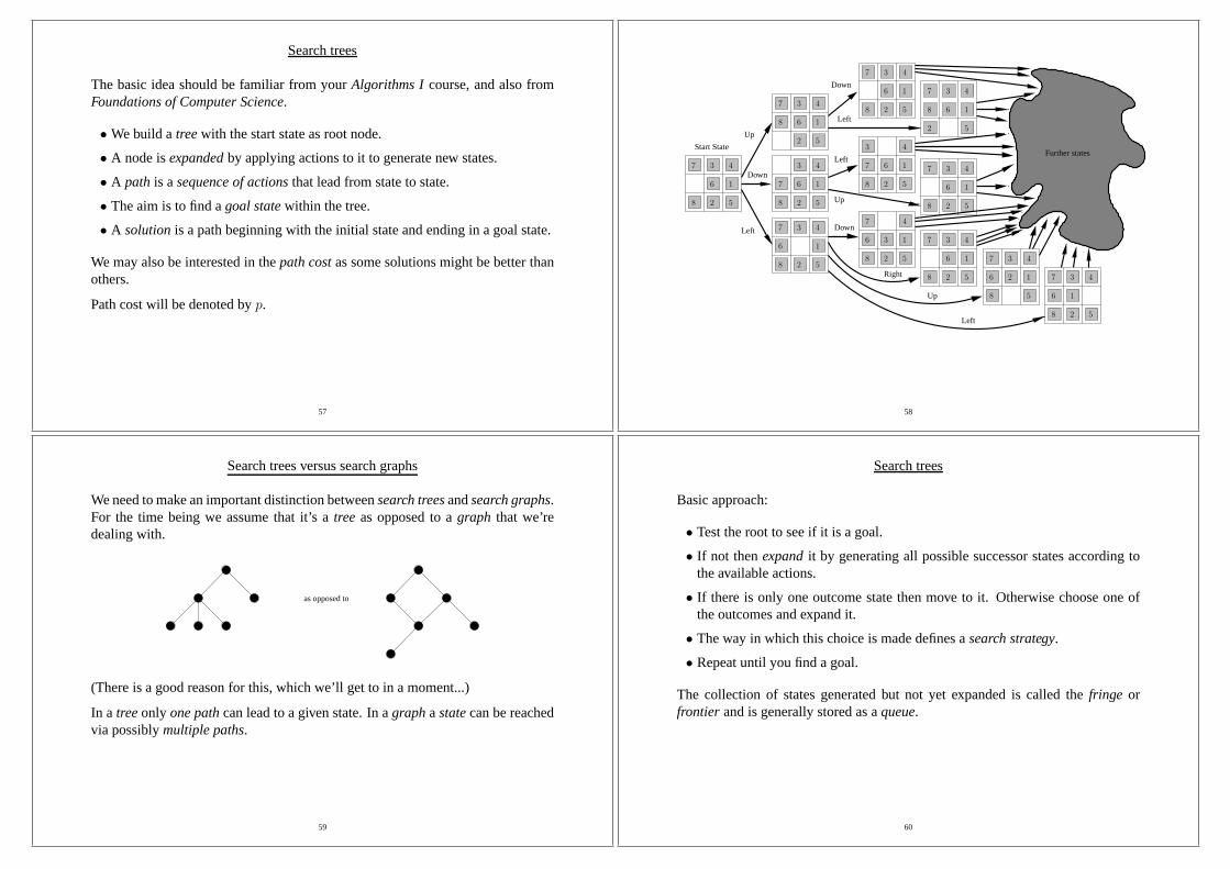
Search trees
The basic idea should be familiar from yourAlgorithms Icourse, and also fromFoundations of Computer Science.
• We build atreewith the start state as root node.
• A node isexpandedby applying actions to it to generate new states.
• A path is asequence of actionsthat lead from state to state.
• The aim is to find agoal statewithin the tree.
• A solutionis a path beginning with the initial state and ending in a goalstate.
We may also be interested in thepath costas some solutions might be better thanothers.
Path cost will be denoted byp.
57
2 58
6
7 3 4
1 7
2 58
6
3 4
1
2 58
6
7 3 4
1
5
6
3
18
7 4
2
7
3
2 58
6
4
1 7
2 58
6
3 4
1
6
2 58
7 3 4
1
6
6
6
2
1
3
2 5
6
7 3 4
18
Start State
2 58
7 4
1
2 58
7 3 4
1
58
7 3 4
1
2 58
7 3 4
6
Further states
Up
Down
Left
Down
Left
Up
Left
Down
Right
Up
Left
58
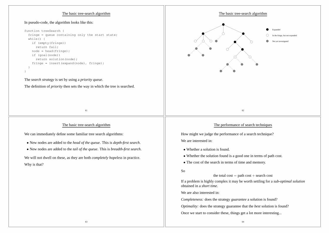
Search trees versus search graphs
We need to make an important distinction betweensearch treesandsearch graphs.For the time being we assume that it’s atree as opposed to agraph that we’redealing with.
as opposed to
(There is a good reason for this, which we’ll get to in a moment...)
In a treeonly one pathcan lead to a given state. In agraphastatecan be reachedvia possiblymultiple paths.
59
Search trees
Basic approach:
• Test the root to see if it is a goal.
• If not thenexpandit by generating all possible successor states according tothe available actions.
• If there is only one outcome state then move to it. Otherwise choose one ofthe outcomes and expand it.
• The way in which this choice is made defines asearch strategy.
• Repeat until you find a goal.
The collection of states generated but not yet expanded is called the fringe orfrontier and is generally stored as aqueue.
60
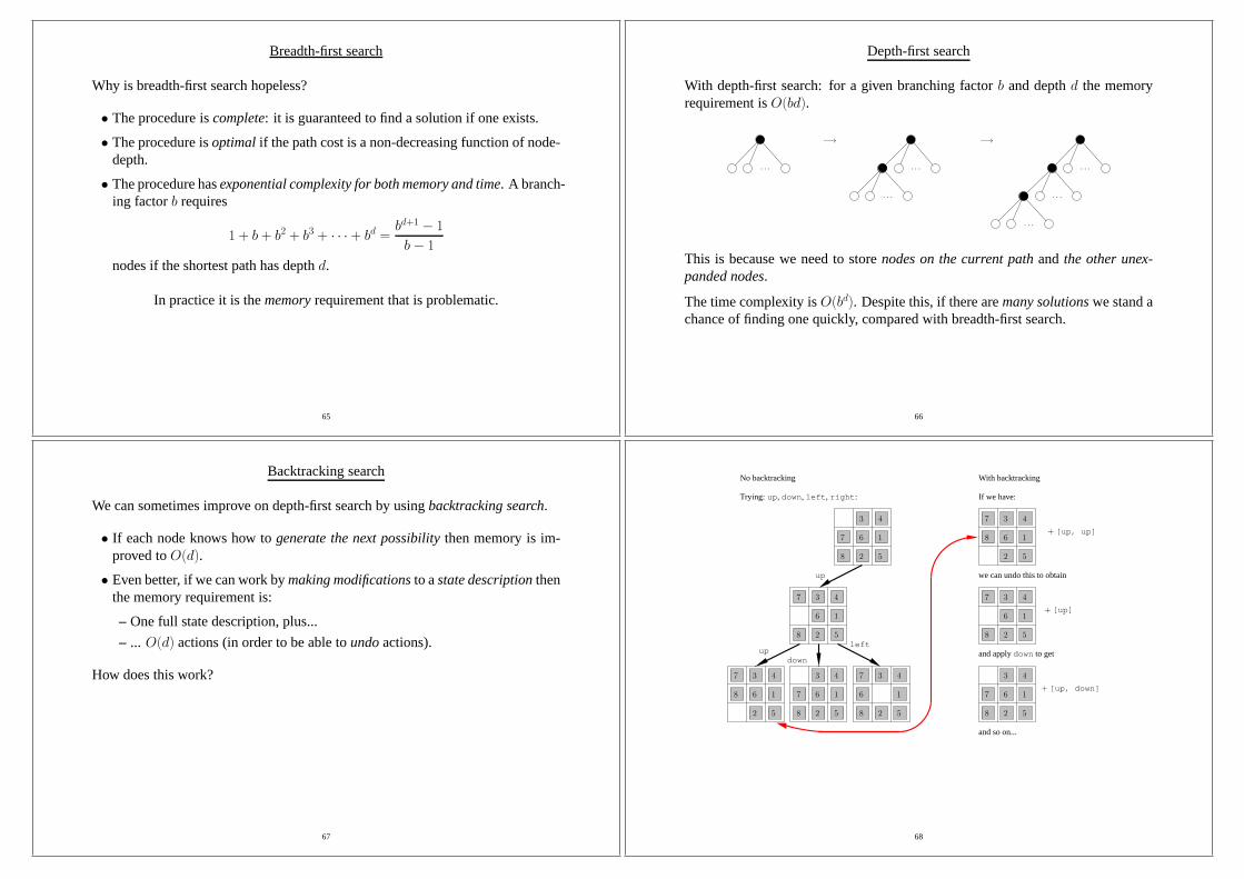
The basic tree-search algorithm
In pseudo-code, the algorithm looks like this:
function treeSearch {fringe = queue containing only the start state;while() {if (empty(fringe))return fail;
node = head(fringe);if (goal(node))return solution(node);
fringe = insert(expand(node), fringe);}
}
Thesearch strategyis set by using apriority queue.
The definition ofpriority then sets the way in which the tree is searched.
61
The basic tree-search algorithm
Not yet investigated
In the fringe, but not expanded
Expanded
62
The basic tree-search algorithm
We can immediately define some familiar tree search algorithms:
• New nodes are added to thehead of the queue. This isdepth-first search.
• New nodes are added to thetail of the queue. This isbreadth-first search.
We will not dwell on these, as they are bothcompletely hopelessin practice.
Why is that?
63
The performance of search techniques
How might we judge the performance of a search technique?
We are interested in:
• Whether a solution is found.
• Whether the solution found is a good one in terms of path cost.
• The cost of the search in terms of time and memory.
Sothe total cost= path cost+ search cost
If a problem is highly complex it may be worth settling for asub-optimal solutionobtained in ashort time.
We are also interested in:
Completeness:does the strategyguaranteea solution is found?
Optimality: does the strategy guarantee that thebestsolution is found?
Once we start to consider these, things get a lot more interesting...
64
Breadth-first search
Why is breadth-first search hopeless?
• The procedure iscomplete: it is guaranteed to find a solution if one exists.
• The procedure isoptimalif the path cost is a non-decreasing function of node-depth.
• The procedure hasexponential complexity for both memory and time. A branch-ing factorb requires
1 + b + b2 + b3 + · · · + bd =bd+1 − 1
b− 1
nodes if the shortest path has depthd.
In practice it is thememoryrequirement that is problematic.
65
Depth-first search
With depth-first search: for a given branching factorb and depthd the memoryrequirement isO(bd).
· · · · · ·
· · ·
· · ·
· · ·
· · ·
−→ −→
This is because we need to storenodes on the current pathand the other unex-panded nodes.
The time complexity isO(bd). Despite this, if there aremany solutionswe stand achance of finding one quickly, compared with breadth-first search.
66
Backtracking search
We can sometimes improve on depth-first search by usingbacktracking search.
• If each node knows how togenerate the next possibilitythen memory is im-proved toO(d).
• Even better, if we can work bymaking modificationsto astate descriptionthenthe memory requirement is:
– One full state description, plus...
– ... O(d) actions (in order to be able toundoactions).
How does this work?
67
2 58
7 3 4
1
2 58
6
3 4
17
6
Trying: up, down, left, right:
No backtracking
+ [up, up]
we can undo this to obtain
+ [up]
and applydown to get
+ [up, down]
and so on...
up
2 58
6
7 3 4
1
2 5
6
7 3 4
18
2 58
6
3 4
17
updown
left
With backtracking
If we have:
2 5
6
7 3 4
18
2 58
7 3 4
1
2 58
6
3 4
17
6
68
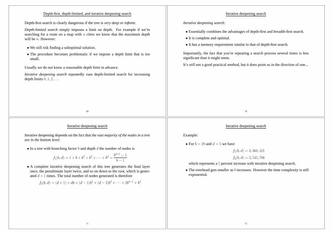
Depth-first, depth-limited, and iterative deepening search
Depth-first search is clearly dangerous if the tree isvery deep or infinite.
Depth-limited searchsimply imposes a limit on depth. For example if we’researching for a route on a map withn cities we know that the maximum depthwill be n. However:
• We still risk finding a suboptimal solution.
• The procedure becomes problematic if we impose a depth limitthat is toosmall.
Usually we do not know a reasonable depth limit in advance.
Iterative deepening searchrepeatedly runs depth-limited search for increasingdepth limits0, 1, 2, . . .
69
Iterative deepening search
Iterative deepening search:
• Essentially combines the advantages of depth-first and breadth-first search.
• It is complete and optimal.
• It has a memory requirement similar to that of depth-first search.
Importantly, the fact that you’re repeating a search process several times is lesssignificant than it might seem.
It’s still not a good practical method, but it does point us in the direction of one...
70
Iterative deepening search
Iterative deepening depends on the fact thatthe vast majority of the nodes in a treeare in the bottom level:
• In a tree with branching factorb and depthd the number of nodes is
f1(b, d) = 1 + b + b2 + b3 + · · · + bd =bd+1 − 1
b− 1
• A complete iterative deepening search of this tree generates the final layeronce, the penultimate layer twice, and so on down to the root,which is gener-atedd + 1 times. The total number of nodes generated is therefore
f2(b, d) = (d + 1) + db + (d− 1)b2 + (d− 2)b3 + · · · + 2bd−1 + bd
71
Iterative deepening search
Example:
• For b = 20 andd = 5 we have
f1(b, d) = 3, 368, 421
f2(b, d) = 3, 545, 706
which represents a5 percent increase with iterative deepening search.
• The overhead getssmallerasb increases. However the time complexity is stillexponential.
72
Iterative deepening search
Further insight can be gained if we note that
f2(b, d) = f1(b, 0) + f1(b, 1) + · · · + f1(b, d)
as we generate the root, then the tree to depth1, and so on. Thus
f2(b, d) =d∑
i=0
f1(b, i) =d∑
i=0
bi+1 − 1
b− 1
=1
b− 1
d∑
i=0
bi+1 − 1 =1
b− 1
[(d∑
i=0
bi+1
)− (d + 1)
]
Noting that
bf1(b, d) = b + b2 + · · · + bd+1 =d∑
i=0
bi+1
we have
f2(b, d) =b
b− 1f1(b, d)−
d + 1
b− 1sof2(b, d) is about equal tof1(b, d) for largeb.
73
Bidirectional search
In some problems we can simultaneously search:
forward from thestart state
backwardfrom thegoalstate
until the searches meet.
This is potentially a very good idea:
• If the search methods have complexityO(bd) then...
• ...we are converting this toO(2bd/2) = O(bd/2).
(Here, we are assuming the branching factor isb in both directions.)
74
Bidirectional search - beware!
• It is not always possible to generate efficientlypredecessorsas well as succes-sors.
• If we only have thedescriptionof a goal, not anexplicit goal, then generatingpredecessors can be hard. (For example, consider the concept of checkmate.)
• We need a way of checking whether or not a node appears in theother search...
• ... and the figure ofO(bd/2) hides the assumption that we can doconstant timechecking for intersection of the frontiers. (This may be possible using a hashtable).
• We need to decide what kind of search to use in each half. For example, woulddepth-first searchbe sensible? Possibly not...
• ...to guarantee that the searches meet, we need to store all the nodes of at leastone of the searches. Consequently the memory requirement isO(bd/2).
75
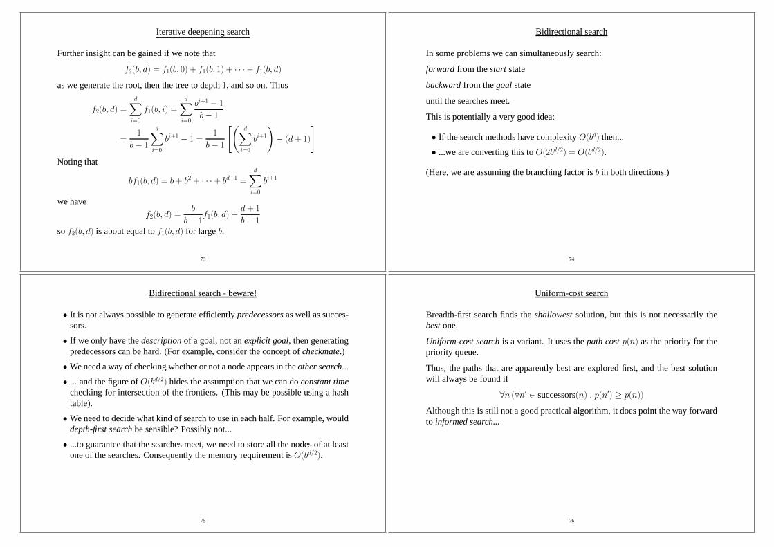
Uniform-cost search
Breadth-first search finds theshallowestsolution, but this is not necessarily thebestone.
Uniform-cost searchis a variant. It uses thepath costp(n) as the priority for thepriority queue.
Thus, the paths that are apparently best are explored first, and the best solutionwill always be found if
∀n (∀n′ ∈ successors(n) . p(n′) ≥ p(n))
Although this is still not a good practical algorithm, it does point the way forwardto informed search...
76

Repeated states
With many problems it is easy to waste time by expanding nodesthat have ap-peared elsewhere in the tree. For example:
.
.
.
.
.
..
.
..
.
..
.
.
A
B
C
D
A
B B
C C CC
The sliding blocks puzzle for example suffers this way.
77
Repeated states
For example, in a problem such as finding a route in a map, whereall of theoperators arereversible, this is inevitable.
There are three basic ways to avoid this, depending on how youtrade off effec-tiveness against overhead.
• Never return tothe state you came from.
• Avoid cycles: never proceed toa state identical to one of your ancestors.
• Do not expandany state that has previously appeared.
Graph searchis a standard approach to dealing with the situation. It usesthe lastof these possibilities.
78
Graph search
In pseudocode:
function graphSearch() {closed = {};fringe = queue containing only the start state;while () {
if (empty(fringe))return fail;
node = head(fringe);if goal(node)return solution(node);
if (node not a member of closed) {closed = closed + node;fringe = insert(expand(node), fringe); // See note...
}}
}
Note: if node is in closed then it must already have been expanded.
79
Graph search
There are several points to note regarding graph search:
1. Theclosed listcontains all the expanded nodes.
2. The closed list can be implemented using a hash table.
3. Both worst case time and space are now proportional to the size of the statespace.
4. Memory:depth first and iterative deepening search are no longer linear spaceas we need to store the closed list.
5. Optimality: when a repeat is found we are discarding the new possibility evenif it is better than the first one.
• This never happens for uniform-cost or breadth-first searchwith constantstep costs, so these remain optimal.
• Iterative deepening search needs to check which solution isbetter and ifnecessary modify path costs and depths for descendants of the repeatedstate.
80
Search trees
Everything we’ve seen so far is an example ofuninformedor blind search—weonly distinguish goal states from non-goal states.
(Uniform cost search is a slight anomaly as it uses the path cost as a guide.)
To perform well in practice we need to employinformedor heuristicsearch.
This involves exploiting knowledge of thedistance between the current state anda goal.
81
Problem solving by informed search
Basic search methods make limited use of anyproblem-specific knowledgewemight have.
• We have already seen the concept ofpath costp(n)
p(n) = cost of path (sequence of actions) from the start state ton
• We can now introduce anevaluation function. This is a function that attemptsto measure thedesirability of each node.
The evaluation function will clearly not be perfect. (If it is, there is no need tosearch.)
Best-first searchsimply expands nodes using the ordering given by the evaluationfunction.
82
Greedy search
We’ve already seenpath costused for this purpose.
• This is misguided as path cost is not in generaldirectedin any sensetowardthe goal.
• A heuristic function, usually denotedh(n) is one thatestimatesthe cost of thebest path from any noden to a goal.
• If n is a goal thenh(n) = 0.
Using a heuristic function along with best-first search gives us thegreedy searchalgorithm.
83
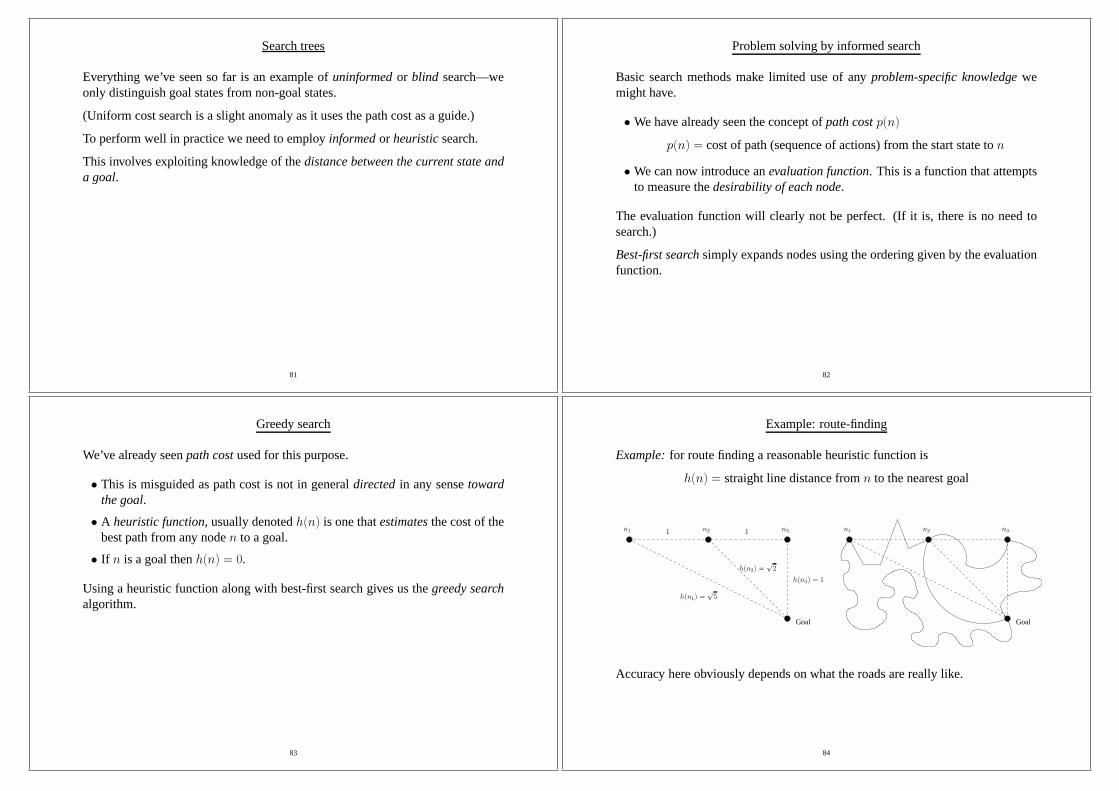
Example: route-finding
Example:for route finding a reasonable heuristic function is
h(n) = straight line distance fromn to the nearest goal
n3
Goal
n1 n21 1
h(n3) = 1
h(n1) =√5
h(n2) =√2
n3
Goal
n1 n2
Accuracy here obviously depends on what the roads are reallylike.
84

Example: route-finding
Greedy search suffers from some problems:
• Its time complexity isO(bd).
• Its space-complexity isO(bd).
• It is not optimal or complete.
BUT: greedy searchcanbe effective, provided we have a goodh(n).
Wouldn’t it be nice if we could improve it to make it optimal and complete?
85
A⋆ search
Well, we can.
A⋆ searchcombines the good points of:
• Greedy search—by making use ofh(n).
• Uniform-cost search—by being optimal and complete.
It does this in a very simple manner: it uses path costp(n) and also the heuristicfunctionh(n) by forming
f(n) = p(n) + h(n)
wherep(n) = cost of pathto n
andh(n) = estimated cost of best pathfromn
So:f(n) is the estimated cost of a paththroughn.
86
A⋆ search
A⋆ search:
• A best-first search usingf(n).
• It is both complete and optimal...
• ...provided thath obeys some simple conditions.
Definition: an admissible heuristich(n) is one thatnever overestimatesthe costof the best path fromn to a goal. So ifh′(n) denotes theactualdistance fromn tothe goal we have
∀n.h(n) ≤ h′(n).
If h(n) is admissible thentree-searchA⋆ is optimal.
87
A⋆ tree-search is optimal for admissibleh(n)
To see thatA⋆ search is optimal we reason as follows.
Let Goalopt be an optimal goal state with
f(Goalopt) = p(Goalopt) = fopt
(becauseh(Goalopt) = 0). Let Goal2 be a suboptimal goal state with
f(Goal2) = p(Goal2) = f2 > fopt
We need to demonstrate that the search can never select Goal2.
88
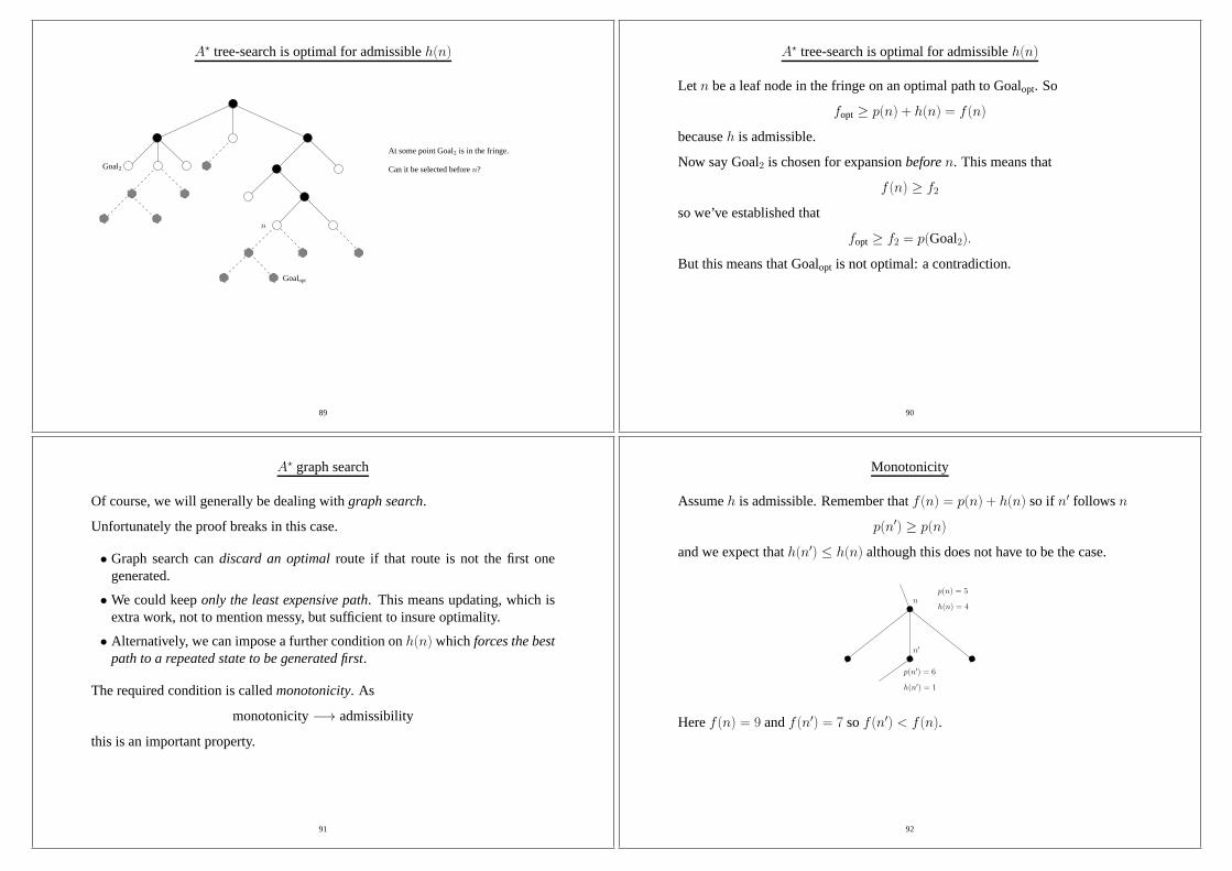
A⋆ tree-search is optimal for admissibleh(n)
Goalopt
n
Goal2
At some point Goal2 is in the fringe.
Can it be selected beforen?
89
A⋆ tree-search is optimal for admissibleh(n)
Let n be a leaf node in the fringe on an optimal path to Goalopt. So
fopt≥ p(n) + h(n) = f(n)
becauseh is admissible.
Now say Goal2 is chosen for expansionbeforen. This means that
f(n) ≥ f2
so we’ve established that
fopt≥ f2 = p(Goal2).
But this means that Goalopt is not optimal: a contradiction.
90
A⋆ graph search
Of course, we will generally be dealing withgraph search.
Unfortunately the proof breaks in this case.
• Graph search candiscard an optimalroute if that route is not the first onegenerated.
• We could keeponly the least expensive path. This means updating, which isextra work, not to mention messy, but sufficient to insure optimality.
• Alternatively, we can impose a further condition onh(n) which forces the bestpath to a repeated state to be generated first.
The required condition is calledmonotonicity. As
monotonicity−→ admissibility
this is an important property.
91
Monotonicity
Assumeh is admissible. Remember thatf(n) = p(n) + h(n) so if n′ follows n
p(n′) ≥ p(n)
and we expect thath(n′) ≤ h(n) although this does not have to be the case.
n
n′
h(n) = 4
p(n′) = 6
h(n′) = 1
p(n) = 5
Heref(n) = 9 andf(n′) = 7 sof(n′) < f(n).
92
Monotonicity
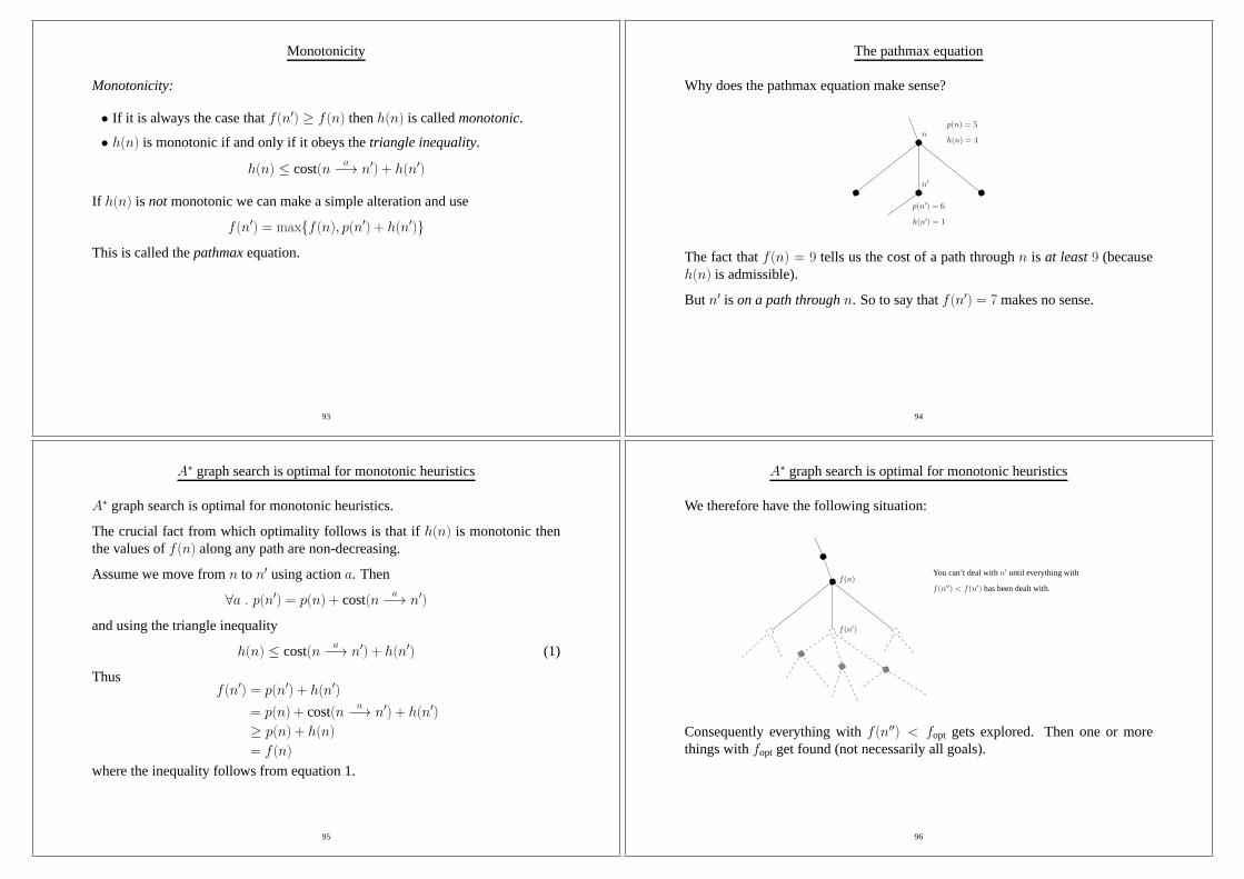
Monotonicity:
• If it is always the case thatf(n′) ≥ f(n) thenh(n) is calledmonotonic.
• h(n) is monotonic if and only if it obeys thetriangle inequality.
h(n) ≤ cost(na−→ n′) + h(n′)
If h(n) is not monotonic we can make a simple alteration and use
f(n′) = max{f(n), p(n′) + h(n′)}This is called thepathmaxequation.
93
The pathmax equation
Why does the pathmax equation make sense?
n
n′
h(n) = 4
p(n′) = 6
h(n′) = 1
p(n) = 5
The fact thatf(n) = 9 tells us the cost of a path throughn is at least9 (becauseh(n) is admissible).
But n′ is on a path throughn. So to say thatf(n′) = 7 makes no sense.
94
A⋆ graph search is optimal for monotonic heuristics
A⋆ graph search is optimal for monotonic heuristics.
The crucial fact from which optimality follows is that ifh(n) is monotonic thenthe values off(n) along any path are non-decreasing.
Assume we move fromn to n′ using actiona. Then
∀a . p(n′) = p(n) + cost(na−→ n′)
and using the triangle inequality
h(n) ≤ cost(na−→ n′) + h(n′) (1)
Thusf(n′) = p(n′) + h(n′)
= p(n) + cost(na−→ n′) + h(n′)
≥ p(n) + h(n)
= f(n)
where the inequality follows from equation 1.
95
A⋆ graph search is optimal for monotonic heuristics
We therefore have the following situation:
f(n)f(n′′) < f(n′) has been dealt with.
f(n′)
You can’t deal withn′ until everything with
Consequently everything withf(n′′) < fopt gets explored. Then one or morethings withfopt get found (not necessarily all goals).
96

A⋆ search is complete
A⋆ search is complete provided:
1. The graph has finite branching factor.
2. There is a finite, positive constantc such that each operator has cost at leastc.
Why is this? The search expands nodes according to increasing f(n). So: theonly way it can fail to find a goal is if there are infinitely manynodes withf(n) <f(Goal).
There are two ways this can happen:
1. There is a node with an infinite number of descendants.
2. There is a path with an infinite number of nodes but a finite path cost.
97
Complexity
• A⋆ search has a further desirable property: it isoptimally efficient.
• This means that no other optimal algorithm that works by constructing pathsfrom the root can guarantee to examine fewer nodes.
• BUT: despite its good properties we’re not done yet...
• ...A⋆ search unfortunately still has exponential time complexity in most casesunlessh(n) satisfies a very stringent condition that is generally unrealistic:
|h(n)− h′(n)| ≤ O(log h′(n))
whereh′(n) denotes thereal cost fromn to the goal.
• As A⋆ search also stores all the nodes it generates, once again it is generallymemory that becomes a problem before time.
98
IDA ⋆ - iterative deepeningA⋆ search
How might we improve the way in whichA⋆ search uses memory?
• Iterative deepening search used depth-first search with a limit on depth that isgradually increased.
• IDA⋆ does the same thingwith a limit onf cost.
ActionSequence ida() {root = root node for problem;float fLimit = f(root);while() {
(sequence, fLimit) = contour(root,fLimit,emptySequence);if (sequence != emptySequence)return sequence;
if (fLimit == infinity)return emptySequence;
}}
99
IDA ⋆ - iterative deepeningA⋆ search
The functioncontour searches from a given node,as far as the specifiedf limit.It returns either a solution, or thenext biggestvalue off to try.
(ActionSequence,float) contour(Node node, float fLimit, ActionSequence s)float nextF = infinity;if (f(node) > fLimit)
return (emptySequence,f(node));ActionSequence s’ = addToSequence(node,s);if (goalTest(node))
return (s’,fLimit);for (each successor n’ of node) {
(sequence,newF) = contour(n’,fLimit,s’);if (sequence != emptySequence)
return (sequence,fLimit);nextF = minimum(nextF,newF);
}return (emptySequence,nextF);
}
100
IDA ⋆ - iterative deepeningA⋆ search
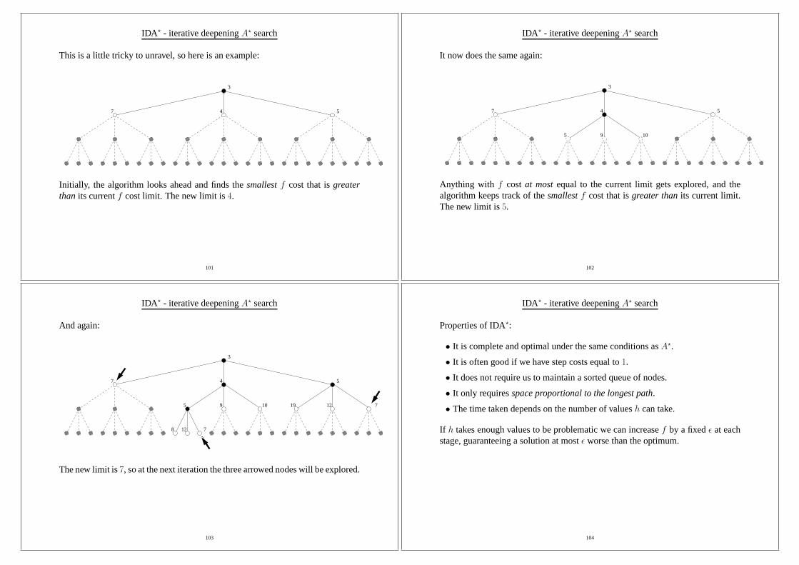
This is a little tricky to unravel, so here is an example:
3
7 4 5
Initially, the algorithm looks ahead and finds thesmallestf cost that isgreaterthan its currentf cost limit. The new limit is4.
101
IDA ⋆ - iterative deepeningA⋆ search
It now does the same again:
3
7 4 5
5 9 10
Anything with f cost at mostequal to the current limit gets explored, and thealgorithm keeps track of thesmallestf cost that isgreater thanits current limit.The new limit is5.
102
IDA ⋆ - iterative deepeningA⋆ search
And again:
3
7 4 5
5 9 10 19 12 7
8 12 7
The new limit is7, so at the next iteration the three arrowed nodes will be explored.
103
IDA ⋆ - iterative deepeningA⋆ search
Properties of IDA⋆:
• It is complete and optimal under the same conditions asA⋆.
• It is often good if we have step costs equal to1.
• It does not require us to maintain a sorted queue of nodes.
• It only requiresspace proportional to the longest path.
• The time taken depends on the number of valuesh can take.
If h takes enough values to be problematic we can increasef by a fixedǫ at eachstage, guaranteeing a solution at mostǫ worse than the optimum.
104
Recursive best-first search (RBFS)
Another method by which we can attempt to overcome memory limitations is theRecursive best-first search (RBFS).
Idea: try to do a best-first search, but only uselinear spaceby doing a depth-firstsearch with a few modifications:
1. We remember thef(n′) for the best alternative noden′ we’ve seen so far onthe way to the noden we’re currently considering.
2. If n hasf(n) > f(n′):
• We go back and explore the best alternative...
• ...and as we retrace our steps we replace thef cost of every node we’veseen in the current path withf(n).
The replacement off values as we retrace our steps provides a means of remem-bering how good a discarded path might be, so that we can easily return to it later.
105
Recursive best-first search (RBFS)
Note: for simplicity a parameter for the path has been omitted.
function RBFS(Node n, Float fLimit) {if (goaltest(n))
return n;if (n has no successors)
return (fail, infinity);for (each successor n’ of n)
f(n’) = maximum(f(n’), f(n));while() {
best = successor of n that has the smallest f(n’);if (f(best) > fLimit)return (fail, f(best));
nextBest = second smallest f(n’) value for successors of n;(result, f’) = RBFS(best, minimum(fLimit, nextBest));f(best) = f’;if (result != fail)return result;
}}
IMPORTANT:f(best) is modifiedwhenRBFS produces a result.
106
Recursive best-first search (RBFS): an example
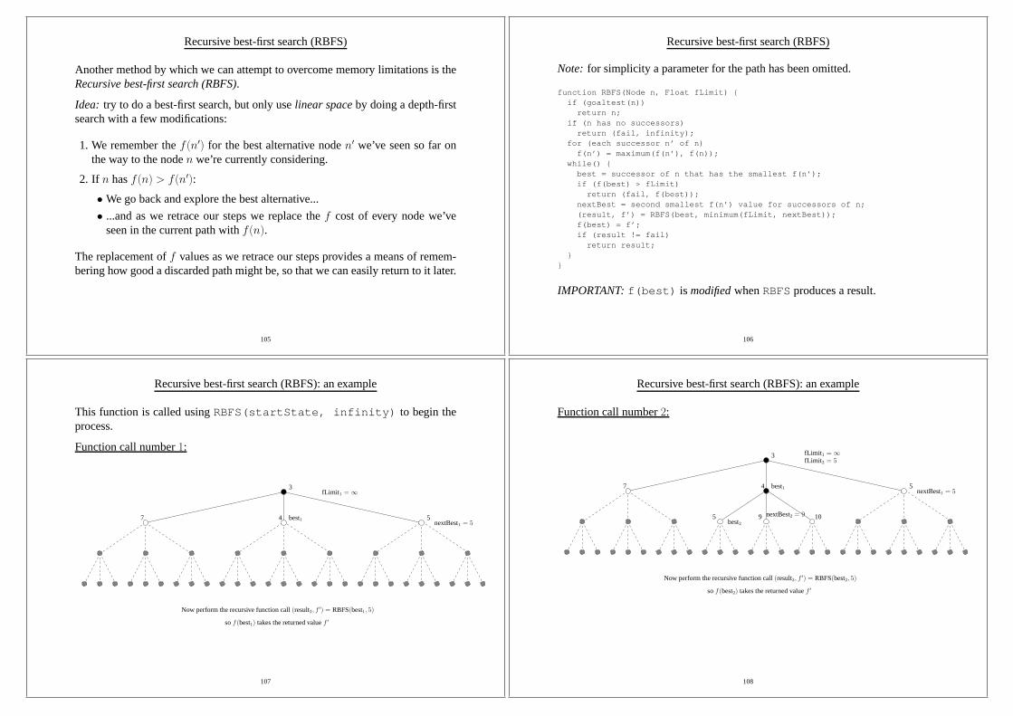
This function is called usingRBFS(startState, infinity) to begin theprocess.
Function call number1:
3
7 4 5best1
fLimit 1 =∞
nextBest1 = 5
Now perform the recursive function call(result2, f ′) = RBFS(best1, 5)
sof(best1) takes the returned valuef ′
107
Recursive best-first search (RBFS): an example
Function call number2:
3
7 4 5best1nextBest1 = 5
fLimit 2 = 5fLimit 1 =∞
5 9 10best2
nextBest2 = 9
Now perform the recursive function call(result3, f ′) = RBFS(best2, 5)
sof(best2) takes the returned valuef ′
108
Recursive best-first search (RBFS): an example
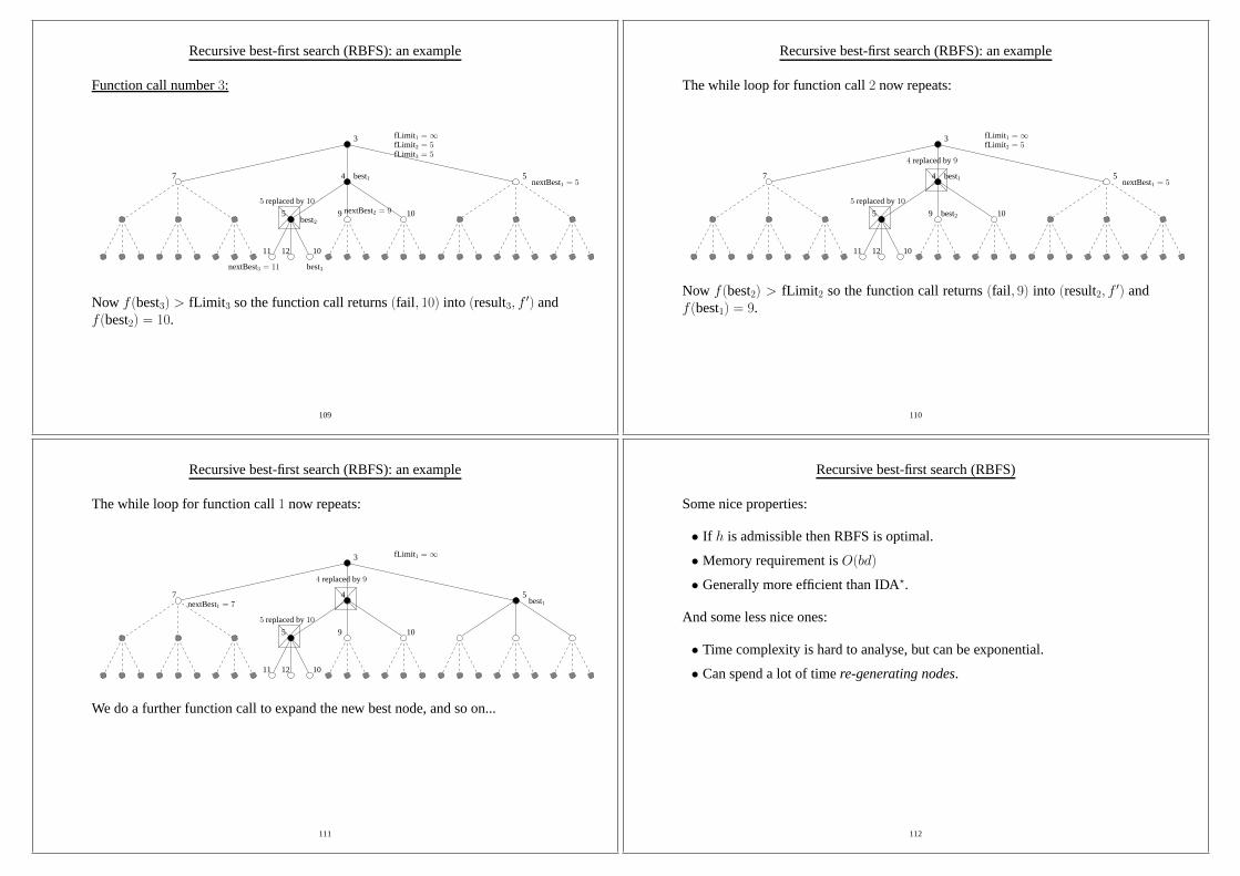
Function call number3:
3
7 4 5best1nextBest1 = 5
fLimit 2 = 5fLimit 1 =∞
5 9 10best2
11 12 10
best3
5 replaced by10nextBest2 = 9
fLimit 3 = 5
nextBest3 = 11
Now f(best3) > fLimit 3 so the function call returns(fail, 10) into (result3, f ′) andf(best2) = 10.
109
Recursive best-first search (RBFS): an example
The while loop for function call2 now repeats:
3
7 4 5best1nextBest1 = 5
fLimit 2 = 5fLimit 1 =∞
5 9 10
11 12 10
5 replaced by10
best2
4 replaced by9
Now f(best2) > fLimit 2 so the function call returns(fail, 9) into (result2, f ′) andf(best1) = 9.
110
Recursive best-first search (RBFS): an example
The while loop for function call1 now repeats:
3
7 4 5
fLimit 1 =∞
5 9 10
11 12 10
5 replaced by10
4 replaced by9
best1nextBest1 = 7
We do a further function call to expand the new best node, and so on...
111
Recursive best-first search (RBFS)
Some nice properties:
• If h is admissible then RBFS is optimal.
• Memory requirement isO(bd)
• Generally more efficient than IDA⋆.
And some less nice ones:
• Time complexity is hard to analyse, but can be exponential.
• Can spend a lot of timere-generating nodes.
112
Other methods for getting around the memory problem
To some extent IDA⋆ and RBFS throw the baby out with the bathwater.
• They limit memory too harshly, so...
• ...we can try to useall available memory.
MA ⋆ and SMA⋆ will not be covered in this course...
113
Local search
Sometimes, it’s only thegoal that we’re interested in. Thepathneeded to get thereis irrelevant.
• For example: VLSI layout, factory design, vehicle routing,automatic pro-gramming...
• We are now simply searching for a node that is in some sensethe best.
• This is also known asoptimisation.
This leads to the remarkably simple concept oflocal search.
114
Local search
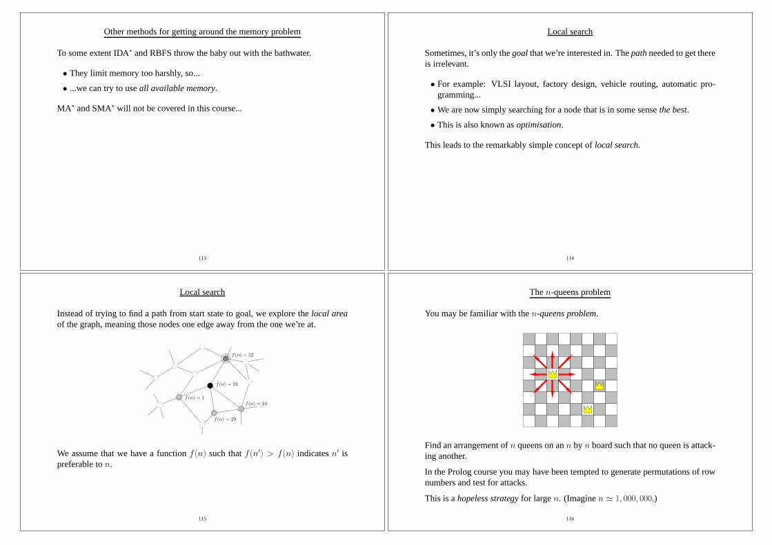
Instead of trying to find a path from start state to goal, we explore thelocal areaof the graph, meaning those nodes one edge away from the one we’re at.
f(n) = 29
f(n) = 1
f(n) = 24
f(n) = 52
f(n) = 24
We assume that we have a functionf(n) such thatf(n′) > f(n) indicatesn′ ispreferable ton.
115
Then-queens problem
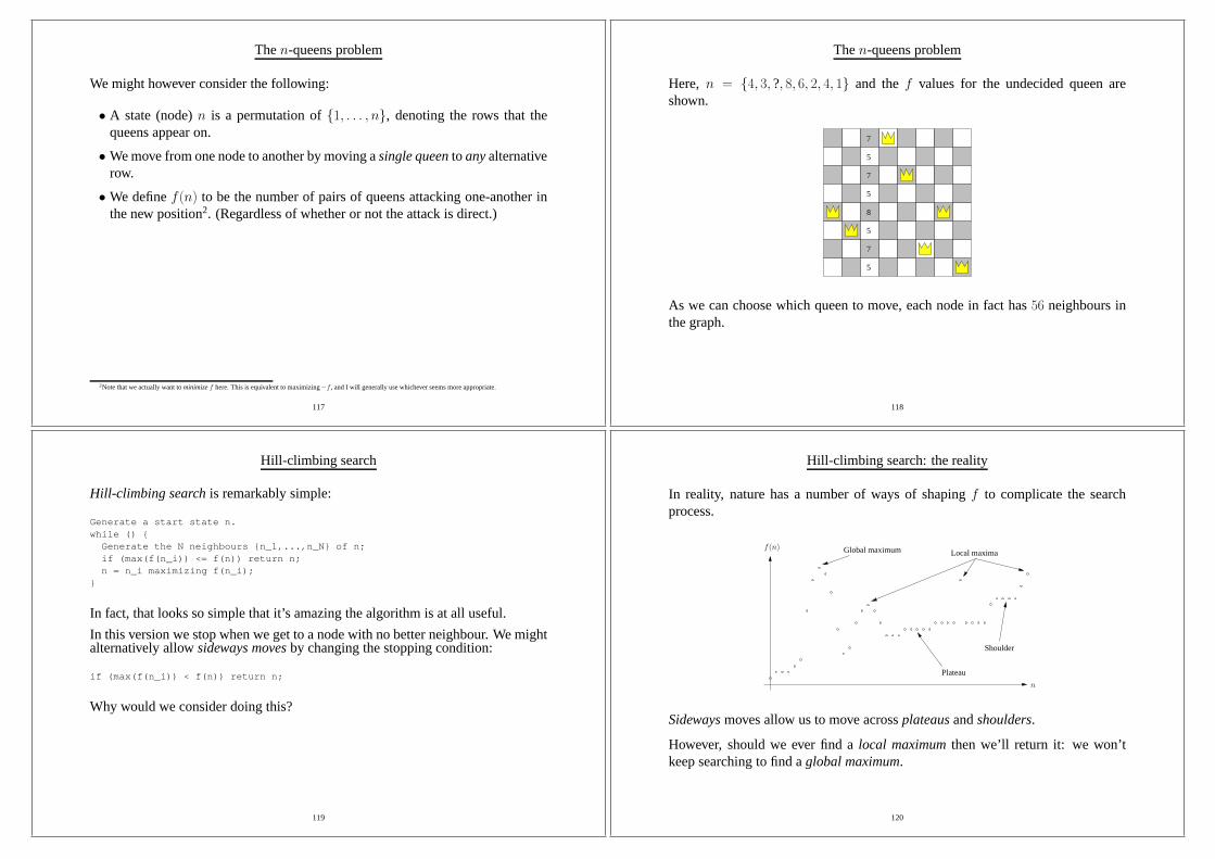
You may be familiar with then-queens problem.
Find an arrangement ofn queens on ann by n board such that no queen is attack-ing another.
In the Prolog course you may have been tempted to generate permutations of rownumbers and test for attacks.
This is ahopeless strategyfor largen. (Imaginen ≃ 1, 000, 000.)
116
Then-queens problem
We might however consider the following:
• A state (node)n is a permutation of{1, . . . , n}, denoting the rows that thequeens appear on.
• We move from one node to another by moving asingle queento anyalternativerow.
• We definef(n) to be the number of pairs of queens attacking one-another inthe new position2. (Regardless of whether or not the attack is direct.)
2Note that we actually want tominimizef here. This is equivalent to maximizing−f , and I will generally use whichever seems more appropriate.
117
Then-queens problem
Here, n = {4, 3, ?, 8, 6, 2, 4, 1} and thef values for the undecided queen areshown.
7
5
7
5
8
5
7
5
As we can choose which queen to move, each node in fact has56 neighbours inthe graph.
118
Hill-climbing search
Hill-climbing searchis remarkably simple:
Generate a start state n.while () {Generate the N neighbours {n_1,...,n_N} of n;if (max(f(n_i)) <= f(n)) return n;n = n_i maximizing f(n_i);
}
In fact, that looks so simple that it’s amazing the algorithmis at all useful.
In this version we stop when we get to a node with no better neighbour. We mightalternatively allowsideways movesby changing the stopping condition:
if (max(f(n_i)) < f(n)) return n;
Why would we consider doing this?
119
Hill-climbing search: the reality
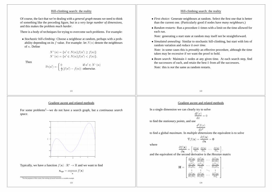
In reality, nature has a number of ways of shapingf to complicate the searchprocess.
Global maximum Local maxima
Plateau
Shoulder
f(n)
n
Sidewaysmoves allow us to move acrossplateausandshoulders.
However, should we ever find alocal maximumthen we’ll return it: we won’tkeep searching to find aglobal maximum.
120
Hill-climbing search: the reality
Of course, the fact that we’re dealing with ageneral graphmeans we need to thinkof something like the preceding figure, but in avery large number of dimensions,and this makes the problemmuch harder.
There is a body of techniques for trying to overcome such problems. For example:
• Stochastic hill-climbing:Choose a neighbour at random, perhaps with a prob-ability depending on itsf value. For example: letN(n) denote the neighboursof n. Define
N+(n) = {n′ ∈ N(n)|f(n′) ≥ f(n)}N−(n) = {n′ ∈ N(n)|f(n′) < f(n)}.
Then
Pr(n′) =
{0 if n′ ∈ N−(n)1Z(f(n′)− f(n)) otherwise.
121
Hill-climbing search: the reality
• First choice:Generate neighbours at random. Select the first one that is betterthan the current one. (Particularly good if nodes havemany neighbours.)
• Random restarts:Run a procedurek times with a limit on the time allowed foreach run.
Note: generating a start state at random may itself not be straightforward.
• Simulated annealing:Similar to stochastic hill-climbing, but start with lots ofrandom variation andreduce it over time.
Note: in some cases this isprovablyan effective procedure, although the timetaken may be excessive if we want the proof to hold.
• Beam search:Maintaink nodes at any given time. At each search step, findthe successors of each, and retain the bestk from all the successors.
Note: this isnot the same as random restarts.
122
Gradient ascent and related methods
For some problems3—we do not have a search graph, but acontinuous searchspace.
0 1 2 3 4 5 6−30
−20
−10
0
10
20
30
x
f(x
)
Typically, we have a functionf(x) : Rn → R and we want to find
xopt = argmaxx
f(x)
3For the purposes of this course, thetraining of neural networksis a notable example.
123
Gradient ascent and related methods
In a single dimension we can clearly try to solvedf(x)
dx= 0
to find thestationary points, and used2f(x)
dx2
to find a globalmaximum. In multiple dimensionsthe equivalent is to solve
∇f(x) = ∂f(x)
∂x= 0
where∂f(x)
∂x=[
∂f(x)∂x1
∂f(x)∂x2· · · ∂f(x)
∂xn
].
and the equivalent of the second derivative is theHessianmatrix
H =
∂f2(x)
∂x21
∂f2(x)∂x1∂x2
· · · ∂f2(x)∂x1∂xn
∂f2(x)∂x2∂x1
∂f2(x)
∂x22· · · ∂f2(x)
∂x2∂xn... ... ... ...
∂f2(x)∂xn∂x1
∂f2(x)∂xn∂x2
· · · ∂f2(x)
∂x2n
.
124
Gradient ascent and related methods
However this approach is usuallynot analytically tractableregardless of dimen-sionality.
The simplest way around this is to employgradient ascent:
• Start with a randomly chosen pointx0.
• Using a smallstep sizeǫ, iterate using the equation
xi+1 = xi + ǫ∇f(xi).
This can be understood as follows:
• At the current pointxi the gradient∇f(xi) tells us thedirectionandmagnitudeof the slope atxi.
• Adding ǫ∇f(xi) therefore moves us asmall distance upward.
This is perhaps more easily seen graphically. . .
125
Gradient ascent and related methods
Here we have a simpleparabolic surface:
−50
0
50
−50
0
50−6000
−4000
−2000
0
2000
x1x2
f(x
)
x1
x2
ǫ = 0.1
−50 0 50−50
0
50
With ǫ = 0.1 the procedure is clearly effective at finding the maximum.
Note however thatthe steps are small, and in a more realistic problemit mighttake some time. . .
126
Gradient ascent and related methods
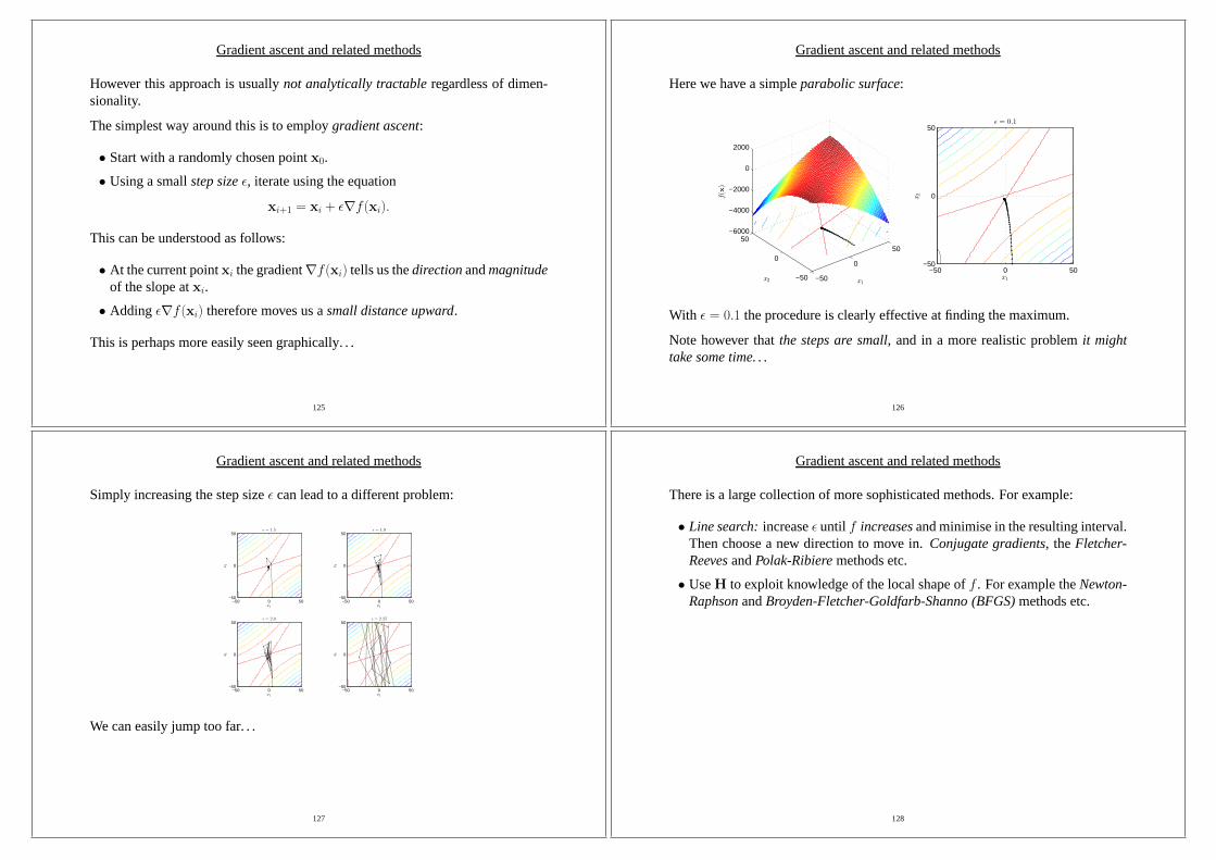
Simply increasing the step sizeǫ can lead to a different problem:
x1
x2
ǫ = 1.5
−50 0 50−50
0
50
x1
x2
ǫ = 1.9
−50 0 50−50
0
50
x1
x2
ǫ = 2.0
−50 0 50−50
0
50
x1
x2
ǫ = 2.25
−50 0 50−50
0
50
We can easily jump too far. . .
127
Gradient ascent and related methods
There is a large collection of more sophisticated methods. For example:
• Line search:increaseǫ until f increasesand minimise in the resulting interval.Then choose a new direction to move in.Conjugate gradients, theFletcher-ReevesandPolak-Ribieremethods etc.
• UseH to exploit knowledge of the local shape off . For example theNewton-RaphsonandBroyden-Fletcher-Goldfarb-Shanno (BFGS)methods etc.
128

Artificial Intelligence I
Dr Sean Holden
Notes ongames (adversarial search)
Copyright c© Sean Holden 2002-2012.
129
Solving problems by search: playing games
How might an agent act whenthe outcomes of its actions are not knownbecauseanadversary is trying to hinder it?
• This is essentially a more realistic kind of search problem because we do notknow the exact outcome of an action.
• This is a common situation whenplaying games: in chess, draughts, and so onan opponentrespondsto our moves.
• We don’t know what their response will be, and so the outcome of our movesis not clear.
Game playing has been of interest in AI because it provides anidealisationof aworld in which two agents act toreduceeach other’s well-being.
130
Playing games: search against an adversary
Despite the fact that games are an idealisation, game playing can be an excellentsource of hard problems. For instance with chess:
• The average branching factor is roughly35.
• Games can reach50 moves per player.
• So a rough calculation gives the search tree35100 nodes.
• Even if only different, legal positions are considered it’sabout1040.
So: in additionto the uncertainty due to the opponent:
• We can’t make a complete search to find the best move...
• ... so we have to act even though we’re not sure about the best thing to do.
131
Playing games: search against an adversary
And chess isn’t even very hard:
• Go is muchharder than chess.
• The branching factor is about360.
Until very recently it has resisted all attempts to produce agood AI player.
See:senseis.xmp.net/?MoGo
and others.
132
Playing games: search against an adversary
It seems that games are a step closer to the complexities inherent in the worldaround us than are the standard search problems considered so far.
The study of games has led to some of the most celebrated applications and tech-niques in AI.
We now look at:
• How game-playing can be modelled assearch.
• Theminimax algorithmfor game-playing.
• Some problems inherent in the use of minimax.
• The concept ofα− β pruning.
Reading:Russell and Norvig chapter 6.
133
Perfect decisions in a two-person game
Say we have two players. Traditionally, they are calledMax andMin for reasonsthat will become clear.
• We’ll usenoughts and crossesas an initial example.
• Max moves first.
• The players alternate until the game ends.
• At the end of the game, prizes are awarded. (Or punishments administered—EVIL ROBOT is starting up his favourite chainsaw...)
This is exactly the same game format as chess, Go, draughts and so on.
134
Perfect decisions in a two-person game
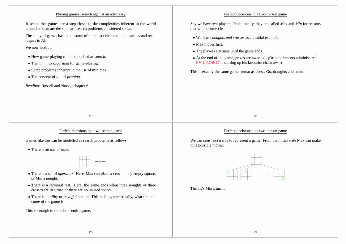
Games like this can be modelled as search problems as follows:
• There is aninitial state.
Max to move
• There is a set ofoperators. Here, Max can place a cross in any empty square,or Min a nought.
• There is aterminal test. Here, the game ends when three noughts or threecrosses are in a row, or there are no unused spaces.
• There is autility or payoff function. This tells us, numerically, what the out-come of the game is.
This is enough to model the entire game.
135
Perfect decisions in a two-person game
We canconstruct a treeto represent a game. From the initial state Max can makenine possible moves:
. . .
Then it’s Min’s turn...
136
Perfect decisions in a two-person game
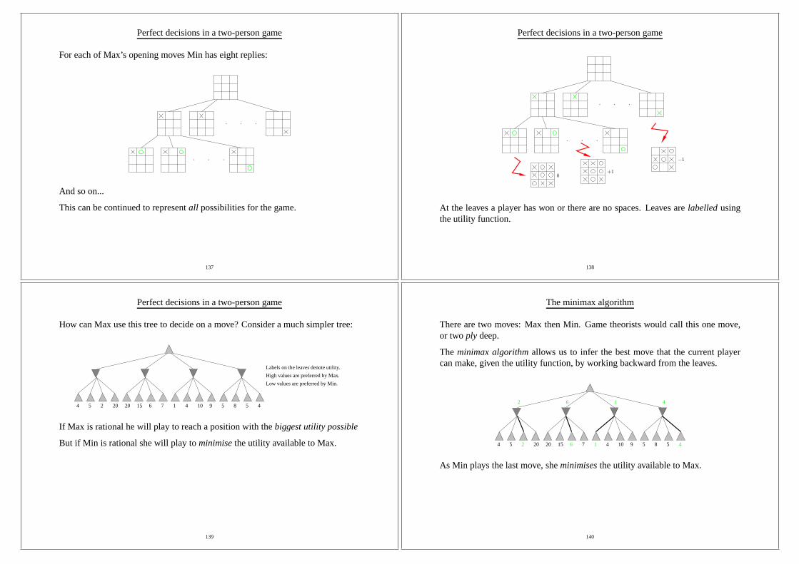
For each of Max’s opening moves Min has eight replies:
. . .
. . .
And so on...
This can be continued to representall possibilities for the game.
137
Perfect decisions in a two-person game
. . .
. . .
+10
−1
At the leaves a player has won or there are no spaces. Leaves are labelledusingthe utility function.
138
Perfect decisions in a two-person game
How can Max use this tree to decide on a move? Consider a much simpler tree:
4 5 2 20 20 15 6 7 1 4 10 9 5 8 5 4
Labels on the leaves denote utility.
High values are preferred by Max.
Low values are preferred by Min.
If Max is rational he will play to reach a position with thebiggest utility possible
But if Min is rational she will play tominimisethe utility available to Max.
139
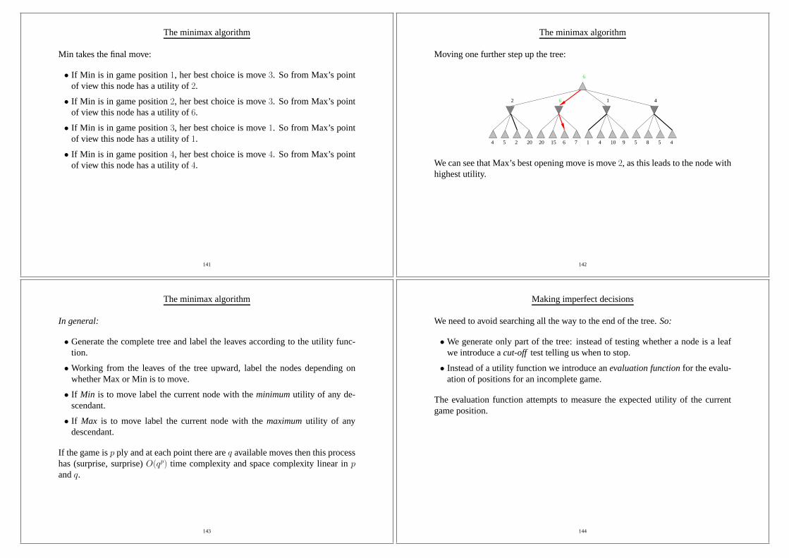
The minimax algorithm
There are two moves: Max then Min. Game theorists would call this one move,or two ply deep.
The minimax algorithmallows us to infer the best move that the current playercan make, given the utility function, by working backward from the leaves.
4 5 20 20 15 7 4 10 9 5 8 52
2
6
6
1
1
4
4
As Min plays the last move, sheminimisesthe utility available to Max.
140
The minimax algorithm
Min takes the final move:
• If Min is in game position1, her best choice is move3. So from Max’s pointof view this node has a utility of2.
• If Min is in game position2, her best choice is move3. So from Max’s pointof view this node has a utility of6.
• If Min is in game position3, her best choice is move1. So from Max’s pointof view this node has a utility of1.
• If Min is in game position4, her best choice is move4. So from Max’s pointof view this node has a utility of4.
141
The minimax algorithm
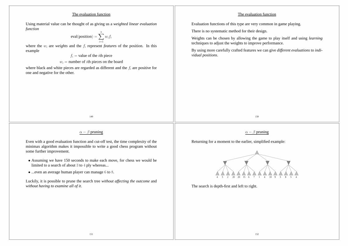
Moving one further step up the tree:
4 5 2 20 20 15 6 7 1 4 10 9 5 8 5 4
1 42 6
6
We can see that Max’s best opening move is move2, as this leads to the node withhighest utility.
142
The minimax algorithm
In general:
• Generate the complete tree and label the leaves according tothe utility func-tion.
• Working from the leaves of the tree upward, label the nodes depending onwhether Max or Min is to move.
• If Min is to move label the current node with theminimumutility of any de-scendant.
• If Max is to move label the current node with themaximumutility of anydescendant.
If the game isp ply and at each point there areq available moves then this processhas (surprise, surprise)O(qp) time complexity and space complexity linear inpandq.
143
Making imperfect decisions
We need to avoid searching all the way to the end of the tree.So:
• We generate only part of the tree: instead of testing whethera node is a leafwe introduce acut-off test telling us when to stop.
• Instead of a utility function we introduce anevaluation functionfor the evalu-ation of positions for an incomplete game.
The evaluation function attempts to measure the expected utility of the currentgame position.
144

Making imperfect decisions
How can this be justified?
• This is a strategy that humans clearly sometimes make use of.
• For example, when using the concept ofmaterial valuein chess.
• The effectiveness of the evaluation function iscritical...
• ... but it must be computable in a reasonable time.
• (In principle it could just be done using minimax.)
The importance of the evaluation function can not be understated—it is probablythe most important part of the design.
145
The evaluation function
Designing a good evaluation function can be extremely tricky:
• Let’s say we want to design one for chess by giving each piece its materialvalue: pawn =1, knight/bishop =3, rook =5 and so on.
• Define the evaluation of a position to be the difference between the materialvalue of black’s and white’s pieces
eval(position) =∑
black’s piecespi
value ofpi −∑
white’s piecesqi
value ofqi
This seems like a reasonable first attempt. Why might it go wrong?
146
The evaluation function
Consider what happens at the start of a game:
• Until the first capture the evaluation function gives0, so in fact we have acat-egorycontaining many different game positions with equal estimated utility.
• For example, all positions where white is one pawn ahead.
• The evaluation function for such a category should perhaps represent the prob-ability that a position chosen at random from it leads to a win.
So in fact this seems highly naive...
147
The evaluation function
Ideally, we should considerindividual positions.
If on the basis of past experience a position has 50% chance ofwinning, 10%chance of losing and 40% chance of reaching a draw, we might give it an evalua-tion of
eval(position) = (0.5× 1) + (0.1×−1) + (0.4× 0) = 0.4.
Extending this to the evaluation of categories, we should then weight the positionsin the category according to their likelihood of occurring.
Of course, wedon’t knowwhat any of these likelihoods are...
148
The evaluation function
Using material value can be thought of as giving us aweighted linear evaluationfunction
eval(position) =n∑
i=1
wifi
where thewi are weightsand thefi representfeaturesof the position. In thisexample
fi = value of theith piece
wi = number ofith pieces on the board
where black and white pieces are regarded as different and the fi are positive forone and negative for the other.
149
The evaluation function
Evaluation functions of this type are very common in game playing.
There is no systematic method for their design.
Weights can be chosen by allowing the game to play itself and using learningtechniques to adjust the weights to improve performance.
By using more carefully crafted features we can givedifferent evaluationsto indi-vidual positions.
150
α− β pruning
Even with a good evaluation function and cut-off test, the time complexity of theminimax algorithm makes it impossible to write a good chess program withoutsome further improvement.
• Assuming we have 150 seconds to make each move, for chess we would belimited to a search of about3 to 4 ply whereas...
• ...even an average human player can manage6 to 8.
Luckily, it is possible to prune the search treewithout affecting the outcomeandwithout having to examine all of it.
151
α− β pruning
Returning for a moment to the earlier, simplified example:
4 5 2 20 20 15 6 7 1 4 10 9 5 8 5 4
The search is depth-first and left to right.
152

α− β pruning
The search continues as previously for the first8 leaves.
4 5 2 20 20 15 6 7 1 4 10 9 5 8 5 4
2 6 ≤ 1
Then we note: ifMax plays move3 thenMin can reach a leaf with utility at most1.
So: we don’t need to search any further under Max’s opening move3. This isbecause the search hasalready establishedthat Max can do better by makingopening move2.
153
α− β pruning in general
Remember that this search isdepth-first. We’re only going to use knowledge ofnodes on the current path.
While searching under this nodewe find that the opponent can forcea score ofn.
If n < m we can stop. There is abetter choice earlier in the game.
If n < m′ we can stop. The playermaximises and will never move here.
of m′.the opponent can force a scoreSearching here establishes that
The value ofα is updated asthe search progresses.
α = m tells us that thevalue of this node is≥ m.
m′
= Player
= Opponentvalue≥ m
value≥ m′
So:once you’ve established thatn is sufficiently small, you don’t need to exploreany more of the corresponding node’s children.
154
α− β pruning in general
The situation is exactly analogous if weswap player and opponentin the previousdiagram.
The search is depth-first, so we’re only ever looking atone path through the tree.
We need to keep track of the valuesα andβ where
α = thehighestutility seen so far on the path forMax
β = the lowestutility seen so far on the path forMin
AssumeMax begins. Initial values forα andβ are
α = −∞and
β = +∞.
155
α− β pruning in general
So: we start with the function call
player(−∞,+∞, root)
The following function implements the procedure suggestedby the previous dia-gram:
player(α, β, n){if (n is at the cut-off point) return evaluation(n);value= −∞;for(each successorn′ of n){
value= max(value, opponent(α, β, n′));if (value> β) return value;if (value> α) α = value;
}return value;}
156
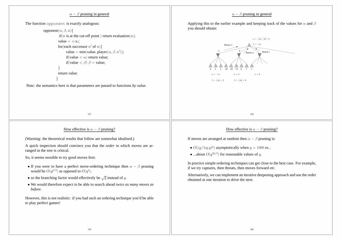
α− β pruning in general
The functionopponent is exactly analogous:
opponent(α, β, n){if (n is at the cut-off point) return evaluation(n);value= +∞;for(each successorn′ of n){
value= min(value,player(α, β, n′));if (value< α) return value;if (value< β) β = value;
}return value;}
Note: the semantics here is that parameters are passed to functions by value.
157
α− β pruning in general
Applying this to the earlier example and keeping track of thevalues forα andβyou should obtain:
4 5 2 20 20 15 6 7 1
2 6
Return2
α = −∞ = 2 = 6
β = +∞
Return6
α = 2
β = +∞ = 6
α = −∞
β = +∞ = 2
α = 6
Return1
158
How effective isα− β pruning?
(Warning: the theoretical results that follow are somewhatidealised.)
A quick inspection should convince you that theorder in which moves are ar-ranged in the tree is critical.
So, it seems sensible to try good moves first:
• If you were to have a perfect move-ordering technique thenα − β pruningwould beO(qp/2) as opposed toO(qp).
• so the branching factor would effectively be√q instead ofq.
• We would therefore expect to be able to search aheadtwice as many moves asbefore.
However, this is not realistic: if you had such an ordering technique you’d be ableto play perfect games!
159
How effective isα− β pruning?
If moves are arranged at random thenα− β pruning is:
• O((q/ log q)p) asymptotically whenq > 1000 or...
• ...aboutO(q3p/4) for reasonable values ofq.
In practice simple ordering techniques can get close to the best case. For example,if we try captures, then threats, then moves forwardetc.
Alternatively, we can implement an iterative deepening approach and use the orderobtained at one iteration to drive the next.
160

A further optimisation: the transposition table
Finally, note that many games correspond tographsrather thantreesbecause thesame state can be arrived at in different ways.
• This is essentially the same effect we saw in heuristic search: recall graphsearchversustree search.
• It can be addressed in a similar way: store a state with its evaluation in a hashtable—generally called atransposition table—the first time it is seen.
The transposition table is essentially equivalent to theclosed listintroduced aspart of graph search.
This can vastly increase the effectiveness of the search process, because we don’thave to evaluate a single state multiple times.
161
Artificial Intelligence I
Dr Sean Holden
Notes onconstraint satisfaction problems (CSPs)
Copyright c© Sean Holden 2002-2012.
162
Constraint satisfaction problems (CSPs)
The search scenarios examined so far seem in some ways unsatisfactory.
• States were represented using anarbitrary andproblem-specificdata structure.
• Heuristics were alsoproblem-specific.
• It would be nice to be able totransformgeneral search problems into astan-dard format.
CSPsstandardisethe manner in which states and goal tests are represented...
163
Constraint satisfaction problems (CSPs)
By standardising like this we benefit in several ways:
• We can devisegeneral purposealgorithms and heuristics.
• We can look at general methods for exploring thestructureof the problem.
• Consequently it is possible to introduce techniques fordecomposingproblems.
• We can try to understand the relationship between thestructureof a problemand thedifficulty of solving it.
Note:another method of interest in AI that allows us to do similar things involvestransforming to apropositional satisfiabilityproblem. We’ll see an example ofthis in AI II.
164
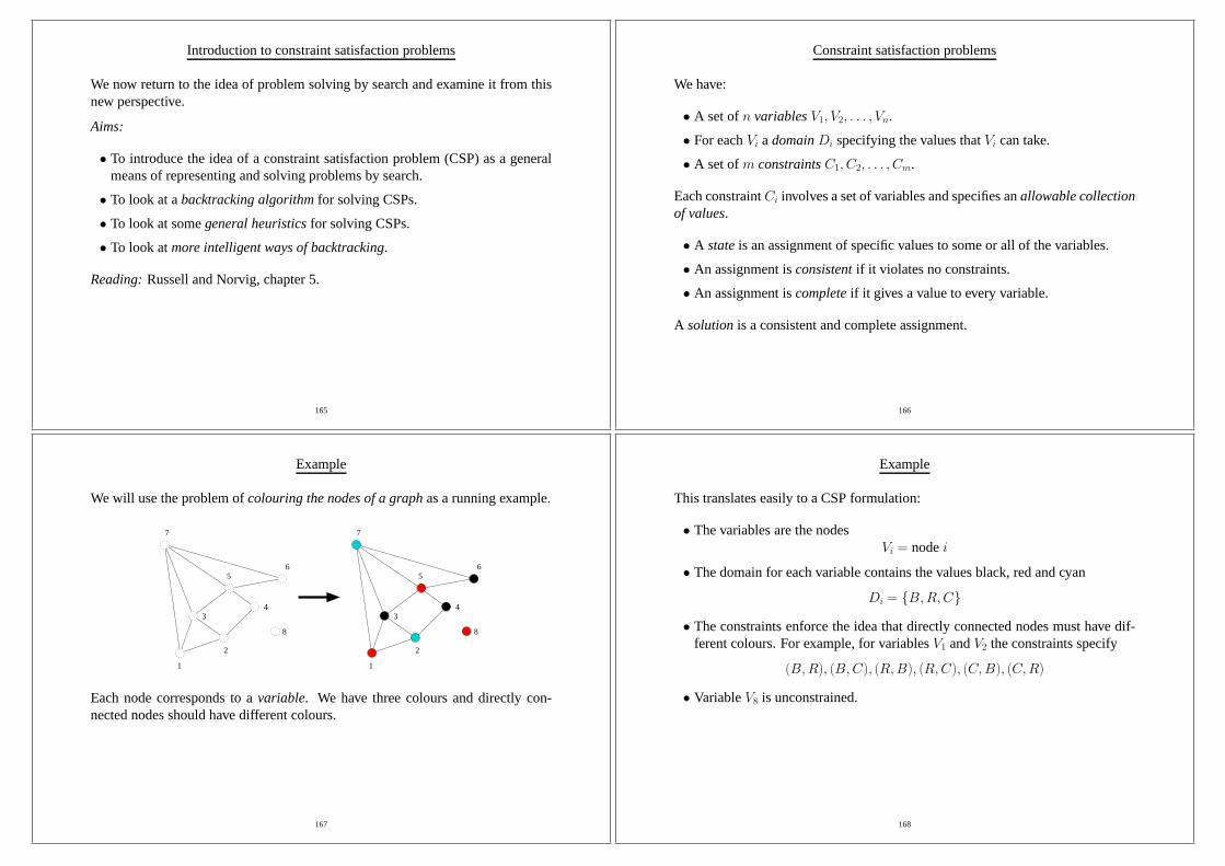
Introduction to constraint satisfaction problems
We now return to the idea of problem solving by search and examine it from thisnew perspective.
Aims:
• To introduce the idea of a constraint satisfaction problem (CSP) as a generalmeans of representing and solving problems by search.
• To look at abacktracking algorithmfor solving CSPs.
• To look at somegeneral heuristicsfor solving CSPs.
• To look atmore intelligent ways of backtracking.
Reading:Russell and Norvig, chapter 5.
165
Constraint satisfaction problems
We have:
• A set ofn variablesV1, V2, . . . , Vn.
• For eachVi a domainDi specifying the values thatVi can take.
• A set ofm constraintsC1, C2, . . . , Cm.
Each constraintCi involves a set of variables and specifies anallowable collectionof values.
• A stateis an assignment of specific values to some or all of the variables.
• An assignment isconsistentif it violates no constraints.
• An assignment iscompleteif it gives a value to every variable.
A solutionis a consistent and complete assignment.
166
Example
We will use the problem ofcolouring the nodes of a graphas a running example.
1
2
8
65
34
7 7
56
43
1
2
8
Each node corresponds to avariable. We have three colours and directly con-nected nodes should have different colours.
167
Example
This translates easily to a CSP formulation:
• The variables are the nodesVi = nodei
• The domain for each variable contains the values black, red and cyan
Di = {B,R,C}
• The constraints enforce the idea that directly connected nodes must have dif-ferent colours. For example, for variablesV1 andV2 the constraints specify
(B,R), (B,C), (R,B), (R,C), (C,B), (C,R)
• VariableV8 is unconstrained.
168

Different kinds of CSP
This is an example of the simplest kind of CSP: it isdiscretewith finite domains.We will concentrate on these.
We will also concentrate onbinary constraints; that is, constraints betweenpairsof variables.
• Constraints on single variables—unary constraints—can be handled by ad-justing the variable’s domain. For example, if we don’t wantVi to bered, thenwe just remove that possibility fromDi.
• Higher-order constraintsapplying to three or more variables can certainly beconsidered, but...
• ...when dealing with finite domains they can always be converted to sets ofbinary constraints by introducing extraauxiliary variables.
How does that work?
169
Auxiliary variables
Example:three variables each with domain{B,R,C}.A single constraint
(C,C,C), (R,B,B), (B,R,B), (B,B,R)
V1 V1V2
V3
The original constraint connects allthree variables.
V2
V3
A = 3
New, binary constraints:
(A = 1, V1 = C), (A = 1, V2 = C), (A = 1, V3 = C)(A = 2, V1 = R), (A = 2, V2 = B), (A = 2, V3 = B)(A = 3, V1 = B), (A = 3, V2 = R), (A = 3, V3 = B)(A = 4, V1 = B), (A = 4, V2 = B), (A = 4, V3 = R)
Introducing auxiliary variableA with domain{1, 2, 3, 4} allows us to convert thisto a set of binary constraints.
170
Backtracking search
Consider what happens if we try to solve a CSP using a simple technique such asbreadth-first search.
The branching factor isnd at the first step, forn variables each withd possiblevalues.
Step 2: (n− 1)dStep 3: (n− 2)d
...Stepn: d
Number of leaves= nd× (n− 1)d× · · · × 1
= n!dn
BUT: only dn assignments are possible.
The order of assignment doesn’t matter, and we should assignto one variable at atime.
171
Backtracking search
Using the graph colouring example:
The search now looks something like this...
1=B1=B1=B2=R 2=R2=R
3=B 3=R 3=C
1=B 1= R 1=C
1=B 1=B 1=B2=B 2=R 2=C
...and new possibilities appear.
172
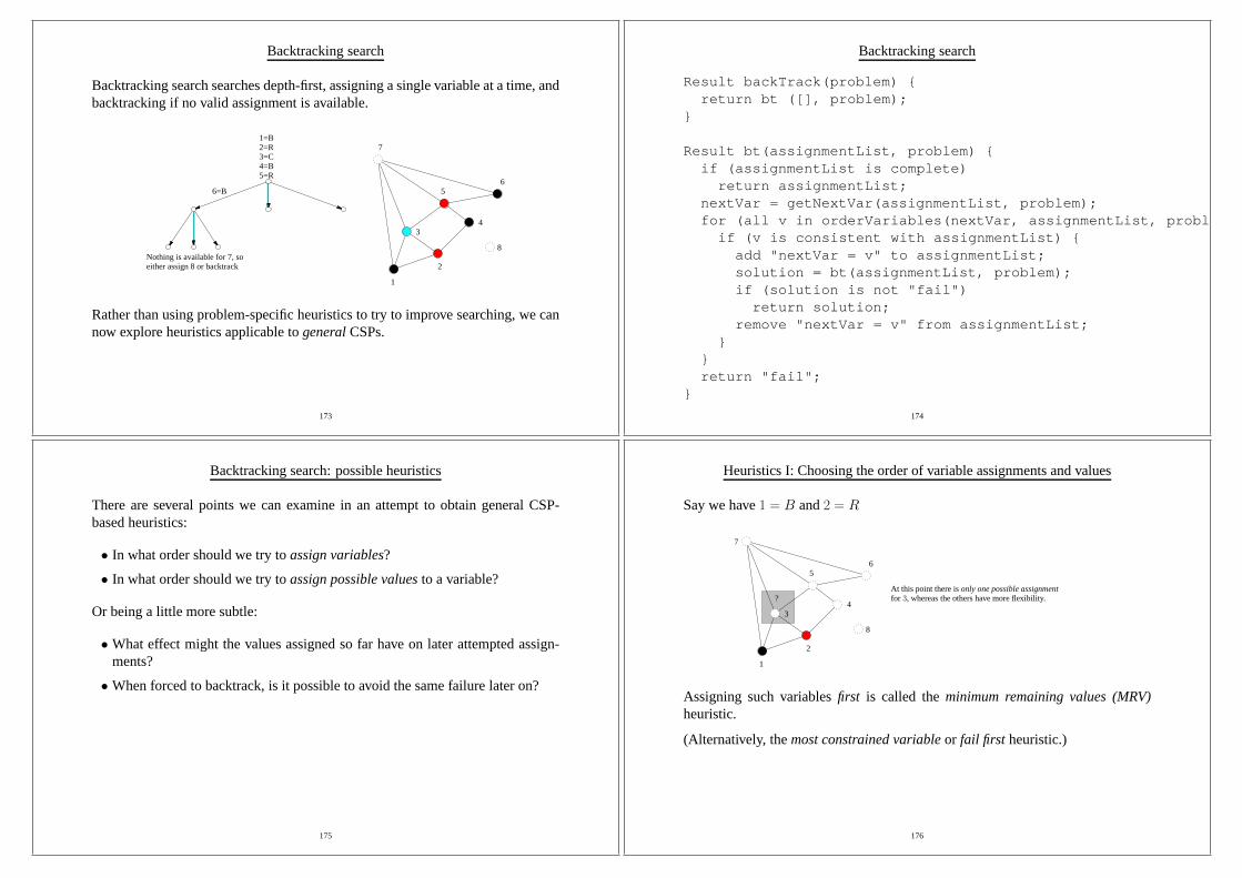
Backtracking search
Backtracking search searches depth-first, assigning a single variable at a time, andbacktracking if no valid assignment is available.
1
2
34
56
7
8
1=B2=R3=C4=B5=R
6=B
Nothing is available for 7, so either assign 8 or backtrack
Rather than using problem-specific heuristics to try to improve searching, we cannow explore heuristics applicable togeneralCSPs.
173
Backtracking search
Result backTrack(problem) {return bt ([], problem);
}
Result bt(assignmentList, problem) {if (assignmentList is complete)
return assignmentList;nextVar = getNextVar(assignmentList, problem);for (all v in orderVariables(nextVar, assignmentList, problem))
if (v is consistent with assignmentList) {add "nextVar = v" to assignmentList;solution = bt(assignmentList, problem);if (solution is not "fail")return solution;
remove "nextVar = v" from assignmentList;}
}return "fail";
}
174
Backtracking search: possible heuristics
There are several points we can examine in an attempt to obtain general CSP-based heuristics:
• In what order should we try toassign variables?
• In what order should we try toassign possible valuesto a variable?
Or being a little more subtle:
• What effect might the values assigned so far have on later attempted assign-ments?
• When forced to backtrack, is it possible to avoid the same failure later on?
175
Heuristics I: Choosing the order of variable assignments and values
Say we have1 = B and2 = R
1
2
34
56
8
?
7
At this point there isonly one possible assignmentfor 3, whereas the others have more flexibility.
Assigning such variablesfirst is called theminimum remaining values (MRV)heuristic.
(Alternatively, themost constrained variableor fail first heuristic.)
176
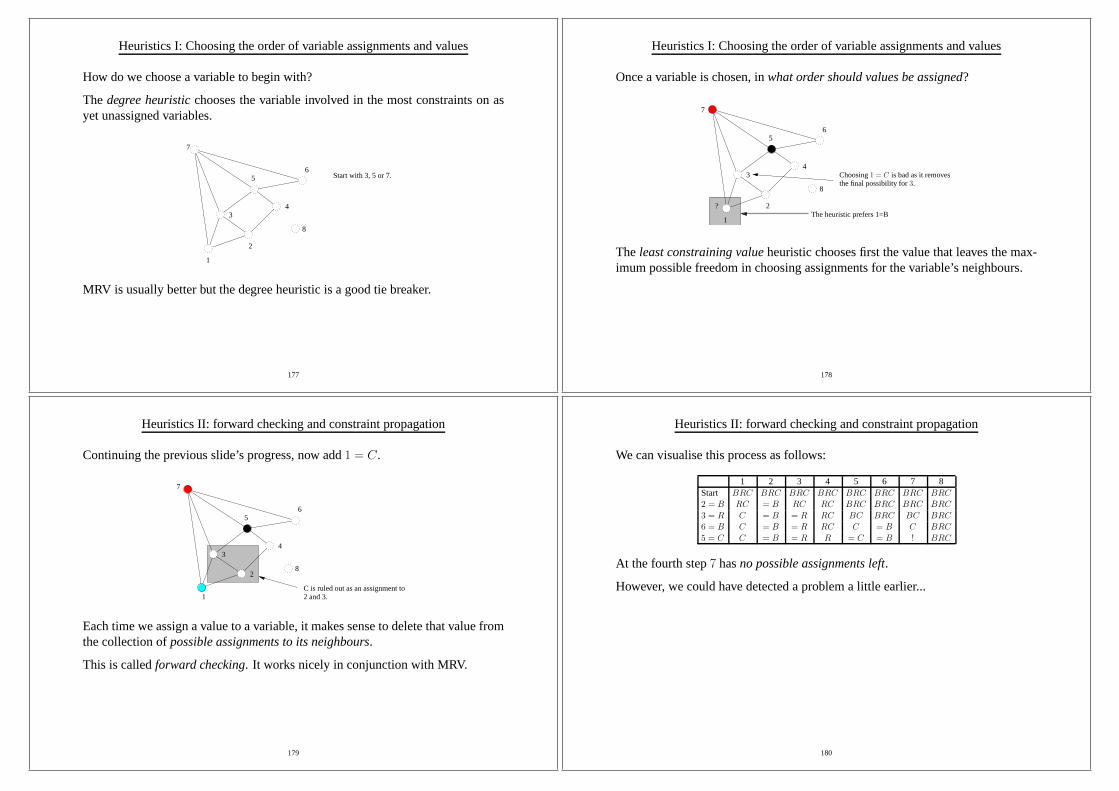
Heuristics I: Choosing the order of variable assignments and values
How do we choose a variable to begin with?
Thedegree heuristicchooses the variable involved in the most constraints on asyet unassigned variables.
1
2
34
56
8
Start with 3, 5 or 7.
7
MRV is usually better but the degree heuristic is a good tie breaker.
177
Heuristics I: Choosing the order of variable assignments and values
Once a variable is chosen, inwhat order should values be assigned?
1
2
34
56
8
?The heuristic prefers 1=B
7
Choosing1 = C is bad as it removesthe final possibility for3.
The least constraining valueheuristic chooses first the value that leaves the max-imum possible freedom in choosing assignments for the variable’s neighbours.
178
Heuristics II: forward checking and constraint propagation
Continuing the previous slide’s progress, now add1 = C.
34
56
8
2 and 3.
7
C is ruled out as an assignment to
2
1
Each time we assign a value to a variable, it makes sense to delete that value fromthe collection ofpossible assignments to its neighbours.
This is calledforward checking. It works nicely in conjunction with MRV.
179
Heuristics II: forward checking and constraint propagation
We can visualise this process as follows:
1 2 3 4 5 6 7 8Start BRC BRC BRC BRC BRC BRC BRC BRC2 = B RC = B RC RC BRC BRC BRC BRC
3 = R C = B = R RC BC BRC BC BRC6 = B C = B = R RC C = B C BRC
5 = C C = B = R R = C = B ! BRC
At the fourth step7 hasno possible assignments left.
However, we could have detected a problem a little earlier...
180

Heuristics II: forward checking and constraint propagation
...by looking at step three.
1 2 3 4 5 6 7 8Start BRC BRC BRC BRC BRC BRC BRC BRC2 = B RC = B RC RC BRC BRC BRC BRC
3 = R C = B = R RC BC BRC BC BRC6 = B C = B = R RC C = B C BRC
5 = C C = B = R R = C = B ! BRC
• At step three,5 can beC only and7 can beC only.
• But 5 and7 are connected.
• So we can’t progress, but this hasn’t been detected.
• Ideally we want to doconstraint propagation.
Trade-off: time to do the search, against time to explore constraints.
181
Constraint propagation
Arc consistency:
Consider a constraint as beingdirected. For example4→ 5.
In general, say we have a constrainti→ j and currently the domain ofi isDi andthe domain ofj is Dj.
i→ j is consistentif
∀d ∈ Di,∃d′ ∈ Dj such thati→ j is valid
182
Constraint propagation
Example:
In step three of the table,D4 = {R,C} andD5 = {C}.
• 5→ 4 in step three of the tableis consistent.
• 4→ 5 in step three of the tableis not consistent.
4→ 5 can be made consistent by deletingC from D4.
Or in other words, regardless of what you assign toi you’ll be able to find some-thing valid to assign toj.
183
Enforcing arc consistency
We can enforce arc consistency each time a variablei is assigned.
• We need to maintain acollection of arcs to be checked.
• Each time we alter a domain, we may have to include further arcs in the col-lection.
This is because ifi→ j is inconsistent resulting in a deletion fromDi we may asa consequence make some arck → i inconsistent.
Why is this?
184

Enforcing arc consistency
with i = R.
{R} kK → i is no longer consistent
i→ j is now consistent.
i→ j is not consistent sodeleteB from the domainof i.
{R} kK → i is consistent butkK = R can only be pairedwith i = B.
becausekK = R can not be paired
{B}{R}{R,B} {B}ji
...
k1
k2
kK
ji...
k1
k2
kK
• i→ j inconsistent means removing a value fromDi.
• ∃d ∈ Di such that there is no validd′ ∈ Dj so deleted ∈ Di.
However somed′′ ∈ Dk may only have been pairable withd.
We need to continue until all consequences are taken care of.
185
The AC-3 algorithm
NewDomains AC-3 (problem) {Queue toCheck = all arcs i->j;while (toCheck is not empty) {i->j = next(toCheck);if (removeInconsistencies(Di,Dj)) {for (each k that is a neighbour of i)add k->i to toCheck;
}}
}
Bool removeInconsistencies (domain1, domain2) {Bool result = false;for (each d in domain1) {if (no d’ in domain2 valid with d) {remove d from domain1;result = true;
}}return result;
}
186
Enforcing arc consistency
Complexity:
• A binary CSP withn variables can haveO(n2) directional constraintsi→ j.
• Any i → j can be considered at mostd times whered = maxk |Dk| becauseonly d things can be removed fromDi.
• Checking any single arc for consistency can be done inO(d2).
So the complexity isO(n2d3).
Note: this setup includes 3SAT.
Consequence:we can’t check for consistency in polynomial time, which suggeststhis doesn’t guarantee to find all inconsistencies.
187
A more powerful form of consistency
We can define a stronger notion of consistency as follows:
• Given: anyk − 1 variables and any consistent assignment to these.
• Then:We can find a consistent assignment to anykth variable.
This is known ask-consistency.
Strongk-consistencyrequires the we bek-consistent,k − 1-consistentetcas fardown as1-consistent.
If we can demonstrate strongn-consistency (where as usualn is the number ofvariables) then an assignment can be found inO(nd).
Unfortunately, demonstrating strongn-consistency will beworst-case exponen-tial.
188
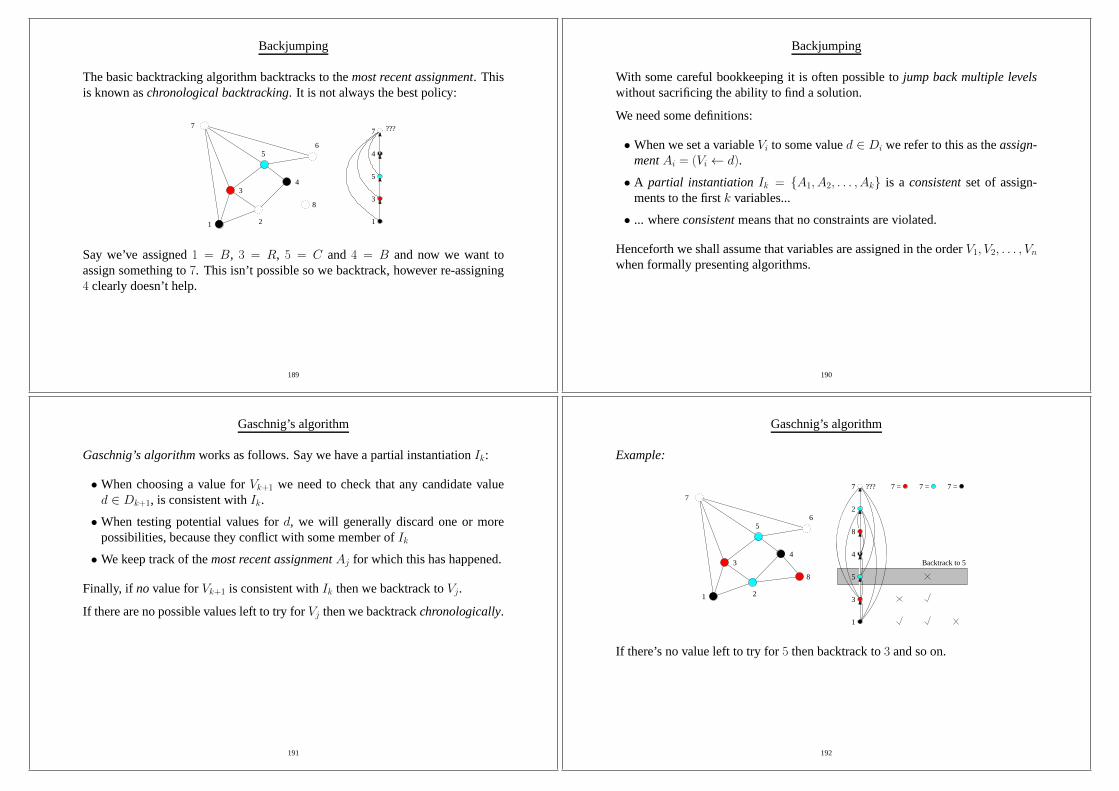
Backjumping
The basic backtracking algorithm backtracks to themost recent assignment. Thisis known aschronological backtracking. It is not always the best policy:
2
34
56
8
7
1
3
5
7
4
1
???
Say we’ve assigned1 = B, 3 = R, 5 = C and 4 = B and now we want toassign something to7. This isn’t possible so we backtrack, however re-assigning4 clearly doesn’t help.
189
Backjumping
With some careful bookkeeping it is often possible tojump back multiple levelswithout sacrificing the ability to find a solution.
We need some definitions:
• When we set a variableVi to some valued ∈ Di we refer to this as theassign-mentAi = (Vi ← d).
• A partial instantiationIk = {A1, A2, . . . , Ak} is a consistentset of assign-ments to the firstk variables...
• ... whereconsistentmeans that no constraints are violated.
Henceforth we shall assume that variables are assigned in the orderV1, V2, . . . , Vn
when formally presenting algorithms.
190
Gaschnig’s algorithm
Gaschnig’s algorithmworks as follows. Say we have a partial instantiationIk:
• When choosing a value forVk+1 we need to check that any candidate valued ∈ Dk+1, is consistent withIk.
• When testing potential values ford, we will generally discard one or morepossibilities, because they conflict with some member ofIk
• We keep track of themost recent assignmentAj for which this has happened.
Finally, if novalue forVk+1 is consistent withIk then we backtrack toVj.
If there are no possible values left to try forVj then we backtrackchronologically.
191
Gaschnig’s algorithm
Example:
2
34
56
8
7
1
1
3
5
4
7
Backtrack to 5
7 = 7 = 7 =
8
2
???
If there’s no value left to try for5 then backtrack to3 and so on.
192

Graph-based backjumping
This allows us to jump back multiple levelswhen we initially detect a conflict.
Can we do better than chronological backtrackingthereafter?
Some more definitions:
• We assume an orderingV1, V2, . . . , Vn for the variables.
• GivenV ′ = {V1, V2, . . . , Vk} wherek < n theancestorsof Vk+1 are the mem-bers ofV ′ connected toVk+1 by a constraint.
• TheparentP (V ) of Vk+1 is its most recent ancestor.
The ancestors for each variable can be accumulated as assignments are made.
Graph-based backjumpingbacktracks to theparentof Vk+1.
193
Graph-based backjumping
2
34
56
8
7
1
1
3
1
3
5
4
1
3
5
1
3
5
4
7
{1}
{3}
{1} {1}
{3}
{5}
{1}
{3}
{5}
{4}
{1, 3, 4, 8}
{1, 3, 5}
8
2
???
At this point, backjump to theparentfor 7, which is5.
194
Backjumping and forward checking
If we useforward checking: say we’re assigning toVk+1 by makingVk+1 = d:
• Forward checking removesd from theDi of all Vi connected toVk+1 by aconstraint.
• When doing graph-based backjumping, we’d also addVk+1 to the ancestors ofVi.
In fact, use of forward checking can make some forms of backjumpingredundant.
Note: there are in fact many ways of combiningconstraint propagationwith back-jumping, and we will not explore them in further detail here.
195
Backjumping and forward checking
2
34
56
8
7
1
3
5
7
4
1
8 − {}
3 − {1}
1 − {}
3
4 − { }
6 − { }7 − {1, , }5
55 − { }3
5
32 − {1, , 4}
Ancestors???
1 2 3 4 5 6 7 8Start BRC BRC BRC BRC BRC BRC BRC BRC1 = B = B RC RC BRC BRC BRC RC BRC
3 = R = B C = R BRC BC BRC C BRC5 = C = B C = R BR = C BR ! BRC4 = B = B C = R BR = C BR ! BRC
Forward checking finds the problembefore backtracking does.
196

Graph-based backjumping
We’re not quite done yet though. What happens whenthere are no assignmentsleft for the parent we just backjumped to?
V4
V3
V2
V1
V7
V6
V5
V4
V3
V2
V1
???
???
Backjumping fromV7 to V4 is fine. However we shouldn’t then just backjump toV2, because changingV3 could fix the problem atV7.
197
Graph-based backjumping
To describe an algorithm in this case is a little involved.
Leaf dead-endI6.
Leaf dead-end variableV7
V4
V3
V2
V1
V6
V5
V4
V3
V2
V1
???
???
Given an instantiationIk andVk+1, if there is no consistentd ∈ Dk+1 we callIk aleaf dead-endandVk+1 a leaf dead-end variable.
198
Graph-based backjumping
Also
Leaf dead-end
Internal dead-endI4.
I6.
Leaf dead-end variableV7
Internal dead-end variableV4V4
V3
V2
V1
V6
V5
V4
V3
V2
V1
???
???
If Vi was backtracked to from a later leaf dead-end and there are nomore valuesto try for Vi then we refer to it as aninternal dead-end variableand callIi−1 aninternal dead-end.
199
Graph-based backjumping
To keep track of exactly where to jump to we also need the definitions:
• Thesessionof a variableV begins when the search algorithm visits it and endswhen it backtracks through it to an earlier variable.
• Thecurrent sessionof a variableV is the set of all variables visiting during itssession.
• In particular, the current session for anyV containsV .
• Therelevant dead-ends for the current sessionR(V ) for a variableV are:
1. If V is a leaf dead-end variable thenR(V ) = {V }.2. If V was backtracked to from a dead-endV ′ thenR(V ) = R(V ) ∪ R(V ′).
And we’re not done yet...
200

Graph-based backjumping
Example:
Session ofV4 = {V4, V5, V6, V7}.
Session starts
Session starts
Session ofV7 = {V7}.R(V7) = {V7}
R(V4) = {V7}
As expected, the relevant dead-end forV4 is {V7}.
201
Graph-based backjumping
One more bunch of definitions before the pain stops. SayVk is a dead-end:
• The induced ancestorsind(Vk) of Vk are defined as
ind(Vk) = {V1, V2, . . . , Vk−1} ∩
⋃
V ∈R(Vk)
ancestors(V )
• Theculprit for Vk is the most recentV ′ ∈ ind(Vk).
Note that these definitions depend onR(Vk).
FINALLY:graph-based backjumpingbackjumps to the culprit.
202
Graph-based backjumping
Example:
Session ofV4 = {V4, V5, V6, V7}.
Backjump fromV7
to V4.
R(V4) = {V7}ind(V4) = {V3}
Nothing left to try!
As expected, we back jump toV3 instead ofV2. Hooray!
203
Conflict-directed backjumping
Gaschnig’s algorithm and graph-based backjumping can becombinedto produceconflict-directed backjumping.
We will not explore conflict-directed backjumping in this course.
For considerable further detail on algorithms for CSPs see:
“Constraint Processing,” Rina Dechter. Morgan Kaufmann, 2003.
204

Varieties of CSP
We have only looked atdiscreteCSPs withfinite domains. These are the simplest.We could also consider:
1. Discrete CSPs withinfinite domains:
• We need aconstraint language. For example
V3 ≤ V10 + 5
• Algorithms are available for integer variables and linear constraints.
• There isno algorithmfor integer variables and nonlinear constraints.
2. Continuous domains—using linear constraints defining convex regions we havelinear programming. This is solvable in polynomial time inn.
3. We can introducepreference constraintsin addition toabsolute constraints,and in some cases anobjective function.
205
Artificial Intelligence I
Dr Sean Holden
Notes onknowledge representation and reasoning using first-order logic (FOL)
Copyright c© Sean Holden 2002-2012.
206
Knowledge representation and reasoning using FOL
We now look at how an agent mightrepresentknowledge about its environmentusing first order logic (FOL), andreasonwith this knowledge to achieve its goals.
Aims:
• To show how FOL can be used torepresent knowledgeabout an environment inthe form of bothbackground knowledgeandknowledge derived from percepts.
• To show how this knowledge can be used toderive non-perceived knowledgeabout the environment using atheorem prover.
• To introduce thesituation calculusand demonstrate its application in a simpleenvironment as a means by which an agent can work out what to donext.
207
Interesting reading
Reading:Russell and Norvig, chapters 7 to 10.
Knowledge representation based on logic is a vast subject and can’t be covered infull in the lectures.
In particular:
• Techniques for representingfurther kinds of knowledge.
• Techniques for moving beyond the idea of asituation.
• Reasoning systems based oncategories.
• Reasoning systems usingdefault information.
• Truth maintenance systems.
Happy reading :-)
208
Knowledge representation and reasoning
Earlier in the course we looked at what anagentshould be able to do.
It seems that all of us—and all intelligent agents—should use logical reasoningto help us interact successfully with the world.
Any intelligent agent should:
• Possessknowledgeabout theenvironmentand abouthow its actions affect theenvironment.
• Use some form oflogical reasoningto maintain its knowledge asperceptsarrive.
• Use some form oflogical reasoningto deduce actionsto perform in order toachievegoals.
209
Knowledge representation and reasoning
This raises some important questions:
• How do we describe the current state of the world?
• How do we infer from our percepts, knowledge of unseen parts of the world?
• How does the world change as time passes?
• How does the world stay the same as time passes? (Theframe problem.)
• How do we know the effects of our actions? (Thequalificationandramifica-tion problems.)
We’ll now look at one way of answering some of these questions.
210
Logic for knowledge representation
FOL (arguably?) seems to provide a good way in which to represent the requiredkinds of knowledge:
• It is expressive—anything you can program can be expressed.
• It is concise.
• It is unambiguous
• It can be adapted todifferent contexts.
• It has aninference procedure, although a semidecidable one.
In addition is has a well-definedsyntaxandsemantics.
211
Logic for knowledge representation
Problem: it’s quite easy to talk about things likeset theoryusing FOL. For exam-ple, we can easily write axioms like
∀S . ∀S ′ . ((∀x . (x ∈ S ⇔ x ∈ S ′))⇒ S = S ′)
But how would we go about representing the proposition thatif you have a bucketof water and throw it at your friend they will get wet, have a bump on their headfrom being hit by a bucket, and the bucket will now be empty anddented?
More importantly, how could this be represented within a wider framework forreasoning about the world?
It’s time to introduce my friend,The Wumpus...
212

Wumpus world
As a simple test scenario for a knowledge-based agent we willmake use of theWumpus World.
Evil Robot
Wumpus
The Wumpus World is a 4 by 4 grid-based cave.
EVIL ROBOT wants to enter the cave, find some gold, and get out again un-scathed.
213
Wumpus world
The rules ofWumpus World:
• Unfortunately the cave contains a number of pits, whichEVIL ROBOT canfall into. Eventually his batteries will fail, and that’s the end of him.
• The cave also contains the Wumpus, who is armed with state of the artEvilRobot Obliteration Technology.
• The Wumpus itself knows where the pits are and never falls into one.
214
Wumpus world
EVIL ROBOT can move around the cave at will and can perceive the following:
• In a position adjacent to the Wumpus, a stench is perceived. (Wumpuses arefamed for theirlack of personal hygiene.)
• In a position adjacent to a pit, abreezeis perceived.
• In the position where the gold is, aglitter is perceived.
• On trying to move into a wall, abumpis perceived.
• On killing the Wumpus ascreamis perceived.
In addition,EVIL ROBOT has a single arrow, with which to try to kill the Wum-pus.
“Adjacent” in the following doesnot include diagonals.
215
Wumpus world
So we have:
Percepts:stench, breeze, glitter, bump, scream.
Actions:forward, turnLeft, turnRight, grab, release, shoot, climb.
Of course, our aim now isnot just to design an agent that can perform well in asingle cave layout.
We want to design an agent that canusuallyperform wellregardlessof the layoutof the cave.
216

Some nomenclature
The choice of knowledge representation language tends to lead to two importantcommitments:
• Ontological commitments: what does the world consist of?
• Epistemological commitments: what are the allowable states of knowledge?
Propositional logic is useful for introducing some fundamental ideas, but its on-tological commitment—that the world consists of facts—sometimes makes it toolimited for further use.
FOL has a different ontological commitment—the world consists offacts, objectsandrelations.
217
Logic for knowledge representation
The fundamental aim is to construct aknowledge baseKB containing acollectionof statementsabout the world—expressed in FOL—such thatuseful things can bederivedfrom it.
Our central aim is to generate sentences that aretrue, if the sentences in theKBare true.
This process is based on concepts familiar from your introductory logic courses:
• Entailment:KB |= α means that theKB entailsα.
• Proof: KB ⊢i α means thatα is derived from theKB usingi. If i is soundthenwe have aproof.
• i is soundif it can generate only entailedα.
• i is completeif it can find a proof foranyentailedα.
218
Example: Prolog
You have by now learned a little about programming inProlog. For example:
concat([],L,L).concat([H|T],L,[H|L2]) :- concat(T,L,L2).
is a program to concatenate two lists. The query
concat([1,2,3],[4,5],X).
results in
X = [1, 2, 3, 4, 5].
What’s happening here? Well, Prolog is just amore limited form of FOLso...
219
Example: Prolog
... we are in fact doing inference from aKB:
• The Prolog programme itself is theKB. It expresses someknowledge aboutlists.
• The query is expressed in such a way as toderive some new knowledge.
How does this relate to full FOL? First of all the list notation is nothing butsyntac-tic sugar. It can be removed: we define a constant calledempty and a functioncalledcons.
Now[1,2,3] just means cons(1, cons(2, cons(3, empty))))whichis a term in FOL.
I will assume the use of the syntactic sugar for lists from nowon.
220

Prolog and FOL
The program when expressed in FOL, says
∀x .concat(empty, x, x)∧∀h, t, l1, l2 .concat(t, l1, l2) =⇒ concat(cons(h, t), l1,cons(h, l2))
The rule is simple—given a Prolog program:
• Universally quantify all the unbound variables in each lineof the programand...
• ... form the conjunction of the results.
If the universally quantified lines areL1, L2, . . . , Ln then the Prolog programmecorresponds to theKB
KB = L1 ∧ L2 ∧ · · · ∧ Ln
Now, what does the query mean?
221
Prolog and FOL
When you give the query
concat([1,2,3],[4,5],X).
to Prolog it responds bytrying to provethe following statement
KB =⇒ ∃x .concat([1, 2, 3], [4, 5], x)So: it tries to prove that theKB implies the query, and variables in the query areexistentially quantified.
When a proof is found, it supplies avalue forx thatmakes the inference true.
222
Prolog and FOL
Prolog differs from FOL in that, amongst other things:
• It restricts you to usingHorn clauses.
• Its inference procedure is not afull-blown proof procedure.
• It does not deal withnegationcorrectly.
Howeverthe central idea also works for full-blown theorem provers.
If you want to experiment, you can obtainProver9from
http://www.cs.unm.edu/∼mccune/mace4/
We’ll see a brief example now, and a more extensive example ofits use later, timepermitting...
223
Prolog and FOL
Expressed in Prover9, the above Prolog program and query look like this:
set(prolog_style_variables).
% This is the translated Prolog program for list concatenation.% Prover9 has its own syntactic sugar for lists.
formulas(assumptions).concat([], L, L).concat(T, L, L2) -> concat([H:T], L, [H:L2]).
end_of_list.
% This is the query.
formulas(goals).exists X concat([1, 2, 3], [4, 5], X).
end_of_list.
Note: it is assumed thatunbound variables are universally quantified.
224

Prolog and FOL
You can try to infer a proof using
prover9 -f file.in
and the result is (in addition to a lot of other information):
1 concat(T,L,L2) -> concat([H:T],L,[H:L2]) # label(non_clause). [assumption].2 (exists X concat([1,2,3],[4,5],X)) # label(non_clause) # label(goal). [goal].3 concat([],A,A). [assumption].4 -concat(A,B,C) | concat([D:A],B,[D:C]). [clausify(1)].5 -concat([1,2,3],[4,5],A). [deny(2)].6 concat([A],B,[A:B]). [ur(4,a,3,a)].7 -concat([2,3],[4,5],A). [resolve(5,a,4,b)].8 concat([A,B],C,[A,B:C]). [ur(4,a,6,a)].9 $F. [resolve(8,a,7,a)].
This shows that a proof is found but doesn’t explicitly give avalue forX—we’llsee how to extract that later...
225
The fundamental idea
So thebasic ideais: build aKB that encodesknowledge about the world, theeffectsof actionsand so on.
TheKB is a conjunction of pieces of knowledge, such that:
• A query regarding what our agent should docan be posed in the form
∃actionList .Goal(... actionList ...)
• Proving that
KB =⇒ ∃actionList .Goal(... actionList ...)
instantiatesactionList to anactual list of actionsthat will achieve a goalrepresented by theGoal predicate.
We sometimes use the notationask andtell to refer toqueryingandadding totheKB.
226
Using FOL in AI: the triumphant return of the Wumpus
We want to be able tospeculateabout the past and aboutpossible futures. So:
Evil Robot
Wumpus
• We includesituationsin the logical language used by ourKB.
• We includeaxiomsin ourKB that relate to situations.
This gives rise tosituation calculus.
227
Situation calculus
In situation calculus:
• The world consists of sequences ofsituations.
• Over time, an agent moves from one situation to another.
• Situations are changed as a result ofactions.
In Wumpus World the actions are:forward, shoot, grab, climb, release,turnRight, turnLeft.
• A situation argumentis added to items that can change over time. For example
At(location, s)
Items that can change over time are calledfluents.
• A situation argument is not needed for things that don’t change. These aresometimes referred to aseternalor atemporal.
228

Representing change as a result of actions
Situation calculus uses a function
result(action, s)
to denote thenewsituation arising as a result of performing the specified action inthe specified situation.
result(grab, s0) = s1result(turnLeft, s1) = s2result(shoot, s2) = s3result(forward, s3) = s4
...
229
Axioms I: possibility axioms
The first kind of axiom we need in aKB specifieswhen particular actions arepossible.
We introduce a predicatePoss(action, s)
denoting that an action can be performed in situations.
We then need apossibility axiomfor each action. For example:
At(l, s) ∧ Available(gold, l, s) =⇒ Poss(grab, s)
Remember thatunbound variables are universally quantified.
230
Axioms II: effect axioms
Given that an action results in a new situation, we can introduceeffect axiomstospecify the properties of the new situation.
For example, to keep track of whetherEVIL ROBOT has the gold we needeffectaxiomsto describe the effect of picking it up:
Poss(grab, s) =⇒ Have(gold, result(grab, s))
Effect axioms describe the way in which the worldchanges.
We would probably also include
¬Have(gold, s0)
in theKB, wheres0 is thestarting state.
Important: we are describingwhat is truein the situation that resultsfrom per-forming an actionin agiven situation.
231
Axioms III: frame axioms
We needframe axiomsto describethe way in which the world stays the same.
Example:
Have(o, s) ∧¬(a = release ∧ o = gold) ∧ ¬(a = shoot ∧ o = arrow)
=⇒ Have(o, result(a, s))
describes the effect ofhaving something and not discarding it.
In a more general setting such an axiom might well look different. For example
¬Have(o, s) ∧(a 6= grab(o) ∨ ¬(Available(o, s) ∧ Portable(o)))=⇒ ¬Have(o, result(a, s))
describes the effect ofnot having something and not picking it up.
232

The frame problem
Theframe problemhas historically been a major issue.
Representational frame problem: a large number of frame axioms are required torepresent the many things in the world which will not change as the result of anaction.
We will see how to solve this in a moment.
Inferential frame problem: when reasoning about a sequence of situations, all theunchanged properties still need to be carried through all the steps.
This can be alleviated usingplanning systemsthat allow us to reason efficientlywhen actions change only a small part of the world. There are also other remedies,which we will not cover.
233
Successor-state axioms
Effect axioms and frame axioms can be combined intosuccessor-state axioms.
One is needed for each predicate that can change over time.
Action a is possible=⇒(true in new situation⇐⇒(you did something to make it true∨it was already true and you didn’t make it false))
For example
Poss(a, s) =⇒(Have(o, result(a, s)) ⇐⇒ ((a = grab ∧ Available(o,s)) ∨(Have(o, s) ∧ ¬(a = release ∧ o = gold) ∧¬(a = shoot ∧ o = arrow))))
234
Knowing where you are
If s0 is the initial situation we know that
At((1, 1), s0)
I amassumingthat we’ve added axioms allowing us to deal with the numbers0 to5 and pairs of such numbers.(Exercise: do this.)
We need to keep track of what way we’re facing. Say north is0, south is2, east is1 and west is3.
facing(s0) = 0
We need to know how motion affects location
forwardResult((x, y),north) = (x, y + 1)
forwardResult((x, y),east) = (x + 1, y)...
andAt(l, s) =⇒ goForward(s) = forwardResult(l, facing(s))
235
Knowing where you are
The concept of adjacency is very important in the Wumpus world
Adjacent(l1, l2) ⇐⇒ ∃d forwardResult(l1, d) = l2
We also know that the cave is4 by 4 and surrounded by walls
WallHere((x, y)) ⇐⇒ (x = 0 ∨ y = 0 ∨ x = 5 ∨ y = 5)
It is only possible to change location by moving, and this only works if you’re notfacing a wall. So...
...we need a successor-state axiom:
Poss(a, s) =⇒At(l, result(a, s)) ⇐⇒ (l = goForward(s)
∧ a = forward
∧ ¬WallHere(l))∨ (At(l, s) ∧ a 6= forward)
236
Knowing where you are
It is only possible to change orientation by turning. Again,we need a successor-state axiom
Poss(a, s) =⇒facing(result(a, s)) = d ⇐⇒
(a = turnRight ∧ d = mod(facing(s) + 1, 4))
∨ (a = turnLeft ∧ d = mod(facing(s)− 1, 4))
∨ (facing(s) = d ∧ a 6= turnRight ∧ a 6= turnLeft)
and so on...
237
The qualification and ramification problems
Qualification problem: we are in general never completely certain what conditionsare required for an action to be effective.
Consider for example turning the key to start your car.
This will lead to problems if important conditions are omitted from axioms.
Ramification problem: actions tend to have implicit consequences that are large innumber.
For example, if I pick up a sandwich in a dodgy sandwich shop, Iwill also bepicking up all the bugs that live in it. I don’t want to model this explicitly.
238
Solving the ramification problem
The ramification problem can be solved bymodifying successor-state axioms.
For example:
Poss(a, s) =⇒(At(o, l, result(a, s)) ⇐⇒
(a = go(l′, l) ∧[o = robot ∨ Has(robot, o, s)]) ∨
(At(o, l, s) ∧[¬∃l′′ . a = go(l, l′′) ∧ l 6= l′′ ∧{o = robot ∨ Has(robot, o, s)}]))
describes the fact that anythingEVIL ROBOT is carrying moves around with him.
239
Deducing properties of the world: causal rules
If you know where you are, then you can think aboutplacesrather than justsitu-ations.
Synchronic rulesrelate properties shared by a single state of the world.
There are two kinds:causalanddiagnostic.
Causal rules: some properties of the world will produce percepts.
WumpusAt(l1) ∧ Adjacent(l1, l2) =⇒ StenchAt(l2)
PitAt(l1) ∧ Adjacent(l1, l2) =⇒ BreezeAt(l2)
Systems reasoning with such rules are known asmodel-basedreasoning systems.
240
Deducing properties of the world: diagnostic rules
Diagnostic rules: infer properties of the world from percepts.
For example:At(l, s) ∧ Breeze(s) =⇒ BreezeAt(l)
At(l, s) ∧ Stench(s) =⇒ StenchAt(l)
These may not be very strong.
The difference between model-based and diagnostic reasoning can be important.For example, medical diagnosis can be done based on symptomsor based on amodel of disease.
241
General axioms for situations and objects
Note: in FOL, if we have two constantsrobot andgold then an interpretationis free to assign them to be the same thing.
This is not something we want to allow.
Unique names axiomsstate that each pair of distinct items in our model of theworld must be different
robot 6= gold
robot 6= arrow
robot 6= wumpus...
wumpus 6= gold...
242
General axioms for situations and objects
Unique actions axiomsstate that actions must share this property, so for each pairof actions
go(l, l′) 6= grab
go(l, l′) 6= drop(o)...
drop(o) 6= shoot...
and in addition we need to define equality for actions, so for each action
go(l, l′) = go(l′′, l′′′) ⇐⇒ l = l′′ ∧ l′ = l′′′
drop(o) = drop(o′) ⇐⇒ o = o′
...
243
General axioms for situations and objects
The situations areorderedso
s0 6= result(a, s)
and situations aredistinctso
result(a, s) = result(a′, s′) ⇐⇒ a = a′ ∧ s = s′
Strictly speaking we should be using amany-sortedversion of FOL.
In such a system variables can be divided intosortswhich are implicitly separatefrom one another.
244
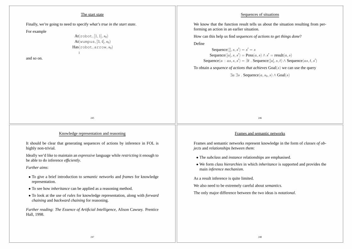
The start state
Finally, we’re going to need to specifywhat’s true in the start state.
For exampleAt(robot, [1, 1], s0)At(wumpus, [3, 4], s0)
Has(robot,arrow, s0)...
and so on.
245
Sequences of situations
We know that the function result tells us about the situationresulting from per-forming an action in an earlier situation.
How can this help us findsequences of actions to get things done?
Define
Sequence([], s, s′) = s′ = s
Sequence([a], s, s′) = Poss(a, s) ∧ s′ = result(a, s)Sequence(a :: as, s, s′) = ∃t . Sequence([a], s, t) ∧ Sequence(as, t, s′)
To obtain asequence of actions that achievesGoal(s) we can use the query
∃a ∃s . Sequence(a, s0, s) ∧Goal(s)
246
Knowledge representation and reasoning
It should be clear that generating sequences of actions by inference in FOL ishighly non-trivial.
Ideally we’d like to maintain anexpressivelanguage whilerestrictingit enough tobe able to do inferenceefficiently.
Further aims:
• To give a brief introduction tosemantic networksand framesfor knowledgerepresentation.
• To see howinheritancecan be applied as a reasoning method.
• To look at the use ofrules for knowledge representation, along withforwardchainingandbackward chainingfor reasoning.
Further reading: The Essence of Artificial Intelligence, Alison Cawsey. PrenticeHall, 1998.
247
Frames and semantic networks
Frames and semantic networks represent knowledge in the form of classes of ob-jectsandrelationships between them:
• Thesubclassandinstancerelationships are emphasised.
• We formclass hierarchiesin which inheritanceis supported and provides themain inference mechanism.
As a result inference is quite limited.
We also need to be extremely careful aboutsemantics.
The only major difference between the two ideas isnotational.
248
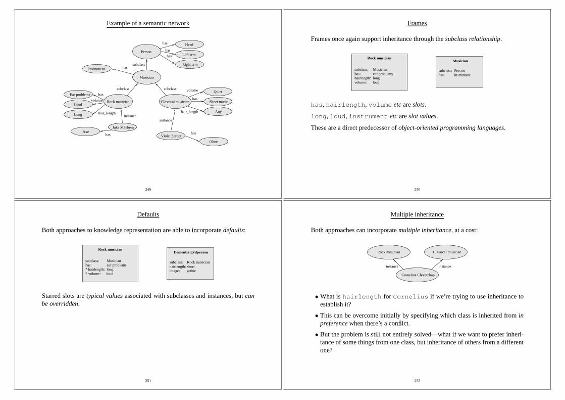
Example of a semantic network
has
Jake Mayhem
instance
Ear problems
volume
has
subclass
Musician
subclasshasInstrument
Person
has
has
Right arm
subclass volume
has
hair_length Any
Sheet music
Quiet
instance
Violet Scroothas
Oboe
has
Axe
Long
LoudRock musician
hair_length
Head
Left arm
Classical musician
249
Frames
Frames once again support inheritance through thesubclass relationship.
volume: loud
has: ear problemshairlength: long
subclass: Musician
Rock musician
subclass: Personhas: instrument
Musician
has, hairlength, volume etcareslots.
long, loud, instrument etcareslot values.
These are a direct predecessor ofobject-oriented programming languages.
250
Defaults
Both approaches to knowledge representation are able to incorporatedefaults:
has: ear problems* hairlength: long
subclass: Musician
* volume: loud
subclass: Rock musicianhairlength: shortimage: gothic
Rock musicianDementia Evilperson
Starred slots aretypical valuesassociated with subclasses and instances, butcanbe overridden.
251
Multiple inheritance
Both approaches can incorporatemultiple inheritance, at a cost:
instanceinstance
Classical musicianRock musician
Cornelius Cleverchap
• What ishairlength for Cornelius if we’re trying to use inheritance toestablish it?
• This can be overcome initially by specifying which class is inherited frominpreferencewhen there’s a conflict.
• But the problem is still not entirely solved—what if we want to prefer inheri-tance of some things from one class, but inheritance of others from a differentone?
252

Other issues
• Slots and slot values can themselves be frames. For exampleDementia mayhave an instrument slot with the valueElectric harp, which itself mayhave properties described in a frame.
• Slots can havespecified attributes. For example, we might specify thatinstrumentcan have multiple values, that each value can only be an instance ofInstrument,that each value has a slot calledowned by and so on.
• Slots may contain arbitrary pieces of program. This is knownasproceduralattachment. The fragment might be executed to return the slot’s value, orupdate the values in other slotsetc.
253
Rule-based systems
A rule-based system requires three things:
1. A set ofif-then rules. These denote specific pieces of knowledge about theworld.
They should be interpreted similarly to logical implication.
Such rules denotewhat to door what can be inferredunder given circum-stances.
2. A collection offactsdenoting what the system regards as currently true aboutthe world.
3. An interpreter able to apply the current rules in the lightof the current facts.
254
Forward chaining
The first of two basic kinds of interpreterbegins with established facts and thenapplies rules to them.
This is adata-drivenprocess. It is appropriate if we know theinitial facts but notthe required conclusion.
Example: XCON—used for configuring VAX computers.
In addition:
• We maintain aworking memory, typically of what has been inferred so far.
• Rules are oftencondition-action rules, where the right-hand side specifies anaction such as adding or removing something from working memory, printinga messageetc.
• In some cases actions might be entire program fragments.
255
Forward chaining
The basic algorithm is:
1. Find all the rules that can fire, based on the current working memory.
2. Select a rule to fire. This requires aconflict resolution strategy.
3. Carry out the action specified, possibly updating the working memory.
Repeat this process until eitherno rules can be usedor ahalt appears in the work-ing memory.
256

Example
dry_mouthworking
InterpreterWorking memory
Condition−action rules
no_work −> DELETE workingworking −> ADD no_workget_drink AND no_work −> ADD go_barthirsty −> ADD get_drinkdry_mouth −> ADD thirsty
257
Example
Progress is as follows:
1. The ruledry mouth =⇒ ADD thirsty
fires addingthirsty to working memory.
2. The rulethirsty =⇒ ADD get drink
fires addingget drink to working memory.
3. The ruleworking =⇒ ADD no work
fires addingno work to working memory.
4. The ruleget drink AND no work =⇒ ADD go bar
fires, and we establish that it’s time to go to the bar.
258
Conflict resolution
Clearly in any more realistic system we expect to have to dealwith a scenariowheretwo or more rules can be fired at any one time:
• Which rule we choose can clearly affect the outcome.
• We might also want to attempt to avoid inferring an abundanceof useless in-formation.
We therefore need a means ofresolving such conflicts.
259
Conflict resolution
Commonconflict resolution strategiesare:
• Prefer rules involving more recently added facts.
• Prefer rules that aremore specific. For example
patient coughing =⇒ ADD lung problem
is more general than
patient coughing AND patient smoker =⇒ ADD lung cancer.
This allows us to define exceptions to general rules.
• Allow the designer of the rules to specify priorities.
• Fire all rulessimultaneously—this essentially involves following all chains ofinference at once.
260

Reason maintenance
Some systems will allow information to be removed from the working memory ifit is no longerjustified.
For example, we might find that
patient coughing
andpatient smoker
are in working memory, and hence fire
patient coughing AND patient smoker =⇒ ADD lung cancer
but later infer something that causespatient coughing to bewithdrawnfromworking memory.
The justification forlung cancer has been removed, and so it should perhapsbe removed also.
261
Pattern matching
In general rules may be expressed in a slightly more flexible form involvingvari-ableswhich can work in conjunction withpattern matching.
For example the rule
coughs(X) AND smoker(X) =⇒ ADD lung cancer(X)
contains the variableX.
If the working memory containscoughs(neddy) andsmoker(neddy) then
X = neddy
provides a match andlung cancer(neddy)
is added to the working memory.
262
Backward chaining
The second basic kind of interpreter begins with agoaland finds a rule that wouldachieve it.
It then worksbackwards, trying to achieve the resulting earlier goals in the suc-cession of inferences.
Example: MYCIN—medical diagnosis with a small number of conditions.
This is agoal-drivenprocess. If you want totest a hypothesisor you have someidea of a likely conclusion it can be more efficient than forward chaining.
263
Example
get drinkno work
thirstyno work
working
dry mouthno work
dry mouthworking
Try first to establishget drink. This
so we’re done.
Working memoryGoal
go bar
can be done by establishingthirsty.
These are the new goals.
establishget drink andno work.
To establishgo bar we have to
thirsty can be established by establishing
dry mouth. This is in the working memory
Finally, we can establishno work by
establishingworking. This is in the working
memory so the process has finished.
264

Example with backtracking
If at some point more than one rule has the required conclusion then we canback-track.
Example: Prolog backtracks, and incorporates pattern matching. It orders at-tempts according to the order in which rules appear in the program.
Example: having added
up early =⇒ ADD tired
andtired AND lazy =⇒ ADD go bar
to the rules, andup early to the working memory:
265
Example with backtracking
thirstyno work
get drinkno work
working
dry mouthno work
dry mouthworkingup early
Process proceeds as before
go bar
lazy
lazyup early
lazytired
different approach.
by establishingtired and
Attempt to establishgo bar
lazy.
This can be done by establishing
up early andlazy.
so we’re done.
up early is in the working memory
We can not establisglazy
and so we backtrack and try a
GoalWorking memory
266
Artificial Intelligence I
Dr Sean Holden
Notes onplanning
Copyright c© Sean Holden 2002-2012.
267
Problem solving is different to planning
In search problemswe:
• Represent states: and a state representation containseverythingthat’s relevantabout the environment.
• Represent actions: by describing a new state obtained from a current state.
• Represent goals: all we know is how to test a state either to see if it’s a goal,or using a heuristic.
• A sequence of actions is a ‘plan’: but we only considersequences of consecu-tive actions.
Search algorithms are good for solving problems that fit thisframework. Howeverfor more complex problems they may fail completely...
268

Problem solving is different to planning
Representing a problem such as:‘go out and buy some pies’is hopeless:
• There aretoo many possible actionsat each step.
• A heuristic can only help you rank states. In particular it does not help youignoreuseless actions.
• We are forced to start at the initial state, but you have to work out how to getthe pies—that is, go to town and buy them, get online and find a web site thatsells piesetc—before you can start to do it.
Knowledge representation and reasoning might not help either: although we endup with a sequence of actions—a plan—there is so much flexibility that complex-ity might well become an issue.
269
Introduction to planning
We now look at how an agent mightconstruct a planenabling it to achieve a goal.
Aims:
• To look at how we might update our concept ofknowledge representation andreasoningto apply more specifically to planning tasks.
• To look in detail at the basicpartial-order planning algorithm.
Reading: Russell and Norvig, chapter 11.
270
Planning algorithms work differently
Difference 1:
• Planning algorithms use aspecial purpose language—often based on FOL ora subset— to represent states, goals, and actions.
• States and goals are described by sentences, as might be expected, but...
• ...actions are described by stating theirpreconditionsand theireffects.
So if you know the goal includes (maybe among other things)
Have(pie)
and action Buy(x) has an effect Have(x) then you know that a planincluding
Buy(pie)
might be reasonable.
271
Planning algorithms work differently
Difference 2:
• Planners can add actions atany relevant point at all between the start and thegoal, not just at the end of a sequence starting at the start state.
• This makes sense: I may determine that Have(carKeys) is a good state to bein without worrying about what happens before or after finding them.
• By making an important decision like requiring Have(carKeys) early on wemay reduce branching and backtracking.
• State descriptions are not complete—Have(carKeys) describes aclass ofstates—and this adds flexibility.
So: you have the potential to search bothforwardsandbackwardswithin the sameproblem.
272

Planning algorithms work differently
Difference 3:
It is assumed that most elements of the environment areindependent of most otherelements.
• A goal including several requirements can be attacked with adivide-and-conquerapproach.
• Each individual requirement can be fulfilled using a subplan...
• ...and the subplans then combined.
This works provided there is not significant interaction between the subplans.
Remember: theframe problem.
273
Running example: gorilla-based mischief
We will use the following simple example problem, which as based on a similarone due to Russell and Norvig.
The intrepid little scamps in theCambridge University Roof-Climbing Societywish to attach aninflatable gorilla to the spire of aFamous College. To do thisthey need to leave home and obtain:
• An inflatable gorilla: these can be purchased from all good joke shops.
• Some rope: available from a hardware store.
• A first-aid kit: also available from a hardware store.
They need to return home after they’ve finished their shopping.
How do they go about planning theirjolly escapade?
274
The STRIPS language
STRIPS:“Stanford Research Institute Problem Solver”(1970).
States: areconjunctionsof ground literals. They must not includefunction sym-bols.
At(home) ∧ ¬Have(gorilla)∧ ¬Have(rope)∧ ¬Have(kit)
Goals: areconjunctionsof literals where variables are assumedexistentially quan-tified.
At(x) ∧ Sells(x,gorilla)
A planner finds a sequence of actions that when performed makes the goal true.We are no longer employing a full theorem-prover.
275
The STRIPS language
STRIPS represents actions usingoperators. For example
At(y),¬At(x)
At(x),Path(x, y)
Go(y)
Op(Action: Go(y),Pre: At(x) ∧ Path(x, y),Effect: At(y) ∧ ¬At(x))
All variables are implicitly universally quantified. An operator has:
• An action description: what the action does.
• A precondition: what must be true before the operator can be used. Acon-junction of positive literals.
• An effect: what is true after the operator has been used. Aconjunction ofliterals.
276

The space of plans
We now make a change in perspective—we search inplan space:
• Start with anempty plan.
• Operate on itto obtain new plans. Incomplete plans are calledpartial plans.Refinement operatorsadd constraints to a partial plan. All other operators arecalledmodification operators.
• Continue until we obtain a plan that solves the problem.
Operations on plans can be:
• Adding a step.
• Instantiating a variable.
• Imposing an orderingthat places a step in front of another.
• and so on...
277
Representing a plan: partial order planners
When putting on your shoes and socks:
• It does not matterwhether you deal with your left or right foot first.
• It does matterthat you place a sock onbeforea shoe, for any given foot.
It makes sense in constructing a plannot to make anycommitmentto which sideis done firstif you don’t have to.
Principle of least commitment: do not commit to any specific choices until youhave to. This can be applied both to ordering and to instantiation of variables. Apartial order plannerallows plans to specify that some steps must come beforeothers but others have no ordering. Alinearisation of such a plan imposes aspecific sequence on the actions therein.
278
Representing a plan: partial order planners
A plan consists of:
1. A set{S1, S2, . . . , Sn} of steps. Each of these is one of the availableoperators.
2. A set ofordering constraints. An ordering constraintSi < Sj denotes the factthat stepSi must happen before stepSj. Si < Sj < Sk and so on has theobvious meaning.Si < Sj doesnot mean thatSi must immediatelyprecedeSj.
3. A set of variable bindingsv = x wherev is a variable andx is either a variableor a constant.
4. A set ofcausal linksor protection intervalsSic→ Sj. This denotes the fact
that the purpose ofSi is to achieve the preconditionc for Sj.
A causal link isalwayspaired with an equivalent ordering constraint.
279
Representing a plan: partial order planners
The initial plan has:
• Two steps, called Start and Finish.
• a single ordering constraint Start< Finish.
• No variable bindings.
• No causal links.
In addition to this:
• The step Start has no preconditions, and its effect is the start state for theproblem.
• The step Finish has no effect, and its precondition is the goal.
• Neither Start or Finish has an associated action.
We now need to consider what constitutes asolution...
280

Solutions to planning problems
A solution to a planning problem is anycompleteandconsistentpartially orderedplan.
Complete: each precondition of each step isachievedby another step in the solu-tion.
A preconditionc for S is achieved by a stepS ′ if:
1. The precondition is an effect of the step
S ′ < S andc ∈ Effects(S ′)
and...
2. ... there isno otherstep thatcould cancel the precondition. That is, noS ′′
exists where:
• The existing ordering constraints allowS ′′ to occurafterS ′ butbeforeS.
• ¬c ∈ Effects(S ′′) .
281
Solutions to planning problems
Consistent: no contradictions exist in the binding constraints or in the proposedordering. That is:
1. For binding constraints, we never havev = X andv = Y for distinct constantsX andY .
2. For the ordering, we never haveS < S ′ andS ′ < S.
Returning to the roof-climber’s shopping expedition, hereis the basic approach:
• Begin with only theStart andFinish steps in the plan.
• At each stage add a new step.
• Always add a new step such that acurrently non-achieved precondition isachieved.
• Backtrack when necessary.
282
An example of partial-order planning
Here is theinitial plan:
Start
Finish
At(Home) ∧ Have(G) ∧ Have(R) ∧ Have(FA)
At(Home)∧ Sells(JS,G) ∧ Sells(HS,R) ∧ Sells(HS,FA)
Thin arrows denote ordering.
283
An example of partial-order planning
There aretwo actions available:
Go(y)
At(y),¬At(x)
Buy(y)
At(x),Sells(x, y)
Have(y)
At(x)
A planner might begin, for example, by adding a Buy(G) action in order to achievethe Have(G) precondition of Finish.
Note: the following order of events is by no means the only one available to aplanner.
It has been chosen for illustrative purposes.
284

An example of partial-order planning
Incorporating the suggested step into the plan:
Start
Buy(G)
Finish
At(Home),Have(G),Have(R),Have(FA)
At(Home),Sells(JS,G),Sells(HS,R),Sells(HS,FA)
At(x),Sells(x,G)
Thick arrows denote causal links. They always have a thin arrow underneath.
Here the newBuy step achieves the Have(G) precondition of Finish.
285
An example of partial-order planning
The planner can now introduce a second causal link from Startto achieve theSells(x,G) precondition of Buy(G).
Start
Buy(G)
Finish
At(Home),Have(G),Have(R),Have(FA)
At(JS),Sells(JS,G)
At(Home),Sells(JS,G),Sells(HS,R),Sells(HS,FA)
286
An example of partial-order planning
The planner’s next obvious move is to introduce a Go step to achieve the At(JS)precondition of Buy(G).
Buy(G)
Finish
At(Home),Have(G),Have(R),Have(FA)
At(Home),Sells(JS,G),Sells(HS,R),Sells(HS,FA)At(x)
Go(JS)
Start
At(JS),Sells(JS,G)
And we continue...
287
An example of partial-order planning
Initially the planner can continue quite easily in this manner:
• Add a causal link from Start to Go(JS) to achieve the At(x) precondition.
• Add the step Buy(R) with an associated causal link to the Have(R) precondi-tion of Finish.
• Add a causal link from Start to Buy(R) to achieve the Sells(HS,R) precondi-tion.
But then things get more interesting...
288
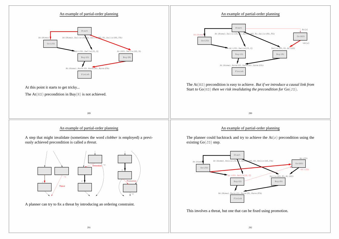
An example of partial-order planning
Start
At(JS),Sells(JS,G)
Finish
At(Home),Have(G),Have(R),Have(FA)
At(Home),Sells(JS,G),Sells(HS,R),Sells(HS,FA)
Buy(R)
At(HS),Sells(HS,R)
At(Home)
Buy(G)
Go(JS)
At this point it starts to get tricky...
The At(HS) precondition in Buy(R) is not achieved.
289
An example of partial-order planning
Start
At(JS),Sells(JS,G)
Finish
At(Home),Have(G),Have(R),Have(FA)
Sells(HS,R),At(HS)
Go(HS)
At(x)
¬At(x)Go(JS)
Buy(G) Buy(R)
At(Home),Sells(JS,G),Sells(HS,R),Sells(HS,FA)At(Home)
The At(HS) precondition is easy to achieve.But if we introduce a causal link fromStartto Go(HS) then we risk invalidating the precondition forGo(JS).
290
An example of partial-order planning
A step that might invalidate (sometimes the wordclobber is employed) a previ-ously achieved precondition is called athreat.
Threat
Promotion
Demotion
c
¬c
cc
¬c
¬c
A planner can try to fix a threat by introducing an ordering constraint.
291
An example of partial-order planning
The planner could backtrack and try to achieve the At(x) precondition using theexisting Go(JS) step.
Start
At(JS),Sells(JS,G)
Go(JS)
Finish
Go(HS)At(Home) At(Home),Sells(JS,G),Sells(HS,R),Sells(HS,FA)
Buy(R)Buy(G)
¬At(JS)
At(JS)
At(Home),Have(G),Have(R),Have(FA)
Sells(HS,R),At(HS)
This involves a threat, but one that can be fixed using promotion.
292

The algorithm
Simplifying slightly to the case where there areno variables.
Say we have a partially completed plan and a set of the preconditions that haveyet to be achieved.
• Select a preconditionp that has not yet been achieved and is associated withan actionB.
• At each stagethe partially complete plan is expanded into a new collection ofplans.
• To expand a plan, we can try to achieve peither by using an action that’salready in the plan or by adding a new action to the plan. In either case, callthe actionA.
We then try to construct consistent plans whereA achievesp.
293
The algorithm
This works as follows:
• Foreach possible way of achievingp:
– Add Start< A, A < Finish,A < B and the causal linkAp→ B to the plan.
– If the resulting plan is consistent we’re done, otherwisegenerate all possi-ble ways of removing inconsistenciesby promotion or demotion andkeepany resulting consistent plans.
At this stage:
• If you haveno further preconditions that haven’t been achievedthenany planobtained is valid.
294
The algorithm
But how do we try toenforce consistency?
When you attempt to achievep usingA:
• Find all the existing causal linksA′¬p→ B′ that areclobberedbyA.
• For each of those you can try addingA < A′ orB′ < A to the plan.
• Find all existing actionsC in the plan that clobber thenewcausal linkAp→ B.
• For each of those you can try addingC < A or B < C to the plan.
• Generateevery possible combinationin this way and retain any consistentplans that result.
295
Possible threats
What about dealing withvariables?
If at any stage an effect¬At(x) appears, is it a threat to At(JS)?
Such an occurrence is called apossible threatand we can deal with it by introduc-ing inequality constraints: in this casex 6= JS.
• Each partially complete plan now has a setI of inequality constraints associ-ated with it.
• An inequality constraint has the formv 6= X wherev is a variable andX is avariable or a constant.
• Whenever we try to make a substitution we checkI to make sure we won’tintroduce a conflict.
If we would introduce a conflict then we discard the partially completedplan asinconsistent.
296

Artificial Intelligence I
Dr Sean Holden
Notes onmachine learning using neural networks
Copyright c© Sean Holden 2002-2012.
297
Did you heed the DIRE WARNING?
At the beginning of the courseI suggested making sure you can answer the fol-lowing two questions:
1. Let
f(x1, . . . , xn) =n∑
i=1
aix2i
where theai are constants. Compute∂f/∂xj where1 ≤ j ≤ n?
Answer:As
f(x1, . . . , xn) = a1x21 + · · · + ajx
2j + · · · + anx
2n
only one term in the sum depends onxj, so all the other terms differentiate togive0 and
∂f
∂xj= 2ajxj
298
Did you heed the DIRE WARNING?
2. Letf(x1, . . . , xn) be a function. Now assumexi = gi(y1, . . . , ym) for eachxiand some collection of functionsgi. Assuming all requirements for differentia-bility and so on are met, can you write down an expression for∂f/∂yj where1 ≤ j ≤ m?
Answer:this is just thechain rulefor partial differentiation
∂f
∂yj=
n∑
i=1
∂f
∂gi
∂gi∂yj
299
Supervised learning with neural networks
We now look at how an agent mightlearn to solve a general problem by seeingexamples.
Aims:
• To present an outline ofsupervised learningas part of AI.
• To introduce much of the notation and terminology used.
• To introduce the classicalperceptron.
• To introducemultilayer perceptronsand thebackpropagation algorithmfortraining them.
Reading: Russell and Norvig chapter 20.
300

An example
A common source of problems in AI ismedical diagnosis.
Imagine that we want to automate the diagnosis of anEmbarrassing Disease(callit D) by constructing a machine:
0 otherwise1 if the patient suffers fromDMeasurementstaken from the
patient: heart rate, blood pressure,presence of green spotsetc.
Machine
Could we do this byexplicitly writing a programthat examines the measurementsand outputs a diagnosis?
Experience suggests that this is unlikely.
301
An example, continued...
An alternative approach: each collection of measurements can be written as avector,
xT = ( x1 x2 · · · xn )
where,
x1 = heart ratex2 = blood pressurex3 = 1 if the patient has green spots
0 otherwise...
and so on
(Note: it’s a common convention that vectors arecolumn vectorsby default. Thisis why the above is written as atranspose.)
302
An example, continued...
A vector of this kind contains all the measurements for a single patient and iscalled afeature vectoror instance.
The measurements areattributesor features.
Attributes or features generally appear as one of three basic types:
• Continuous: xi ∈ [xmin, xmax] wherexmin, xmax∈ R.
• Binary: xi ∈ {0, 1} or xi ∈ {−1,+1}.• Discrete: xi can take one of a finite number of values, sayxi ∈ {X1, . . . , Xp}.
303
An example, continued...
Now imagine that we have a large collection of patient histories (m in total) andfor each of these we know whether or not the patient suffered fromD.
• Theith patient history gives us an instancexi.
• This can be paired with a single bit—0 or 1—denoting whether or not theithpatient suffers fromD. The resulting pair is called anexampleor a labelledexample.
• Collecting all the examples together we obtain atraining sequence
s = ((x1, 0), (x2, 1), . . . , (xm, 0))
304

An example, continued...
In supervised machine learning we aim to design alearning algorithmwhich takess and produces ahypothesish.
Learning Algorithms h
Intuitively, a hypothesis is something that lets us diagnose newpatients.
This isIMPORTANT: we want to diagnose patients thatthe system has never seen.
The ability to do this successfully is calledgeneralisation.
305
An example, continued...
In fact, a hypothesis is just afunctionthat mapsinstancesto labels.
x
Classifier
h(x) LabelAttribute vector
As h is a functionit assigns a label toanyx andnot just the ones that were in thetraining sequence.
What we mean by alabel here depends on whether we’re doingclassificationorregression.
306
Supervised learning: classification
In classificationwe’re assigningx to one of a set{ω1, . . . , ωc} of c classes.
For example, ifx contains measurements taken from a patient then there mightbethree classes:
ω1 = patient has diseaseω2 = patient doesn’t have diseaseω3 = don’t ask me buddy, I’m just a computer!
Thebinary case above also fits into this framework, and we’ll often specialise tothe case of two classes, denotedC1 andC2.
307
Supervised learning: regression
In regressionwe’re assigningx to areal numberh(x) ∈ R.
For example, ifx contains measurements taken regarding today’s weather then wemight have
h(x) = estimate of amount of rainfall expected tomorrow
For the two-class classification problem we will also refer to a situation somewhatbetween the two, where
h(x) = Pr(x is inC1)
and so we would typically assignx to classC1 if h(x) > 1/2.
308

Summary
We don’t want to designh explicitly.
Training sequence
h = L(s)
Labelh(x)
s
LearnerL
ClassifierAttribute vector
x
So we use alearnerL to infer it on the basis of a sequences of training examples.
309
Neural networks
There is generally a setH of hypotheses from whichL is allowed to selecth
L(s) = h ∈ HH is called thehypothesis space.
The learner can output a hypothesis explicitly or—as in the case of aneural net-work—it can output a vector
wT =(w1 w2 · · · wW
)
of weightswhich in turn specifyh
h(x) = f(w;x)
wherew = L(s).
310
Types of learning
The form of machine learning described is calledsupervised learning.
This introduction will concentrate on this kind of learning. In particular, the liter-ature also discusses:
1. Unsupervised learning.
2. Learning usingmembership queriesandequivalence queries.
3. Reinforcement learning.
Some of this further material will be covered in AI 2.
311
Some further examples
• Speech recognition.
• Decidingwhether or not to give credit.
• Detectingcredit card fraud.
• Deciding whether tobuy or sell a stock option.
• Deciding whether atumour is benign.
• Data mining: extracting interesting but hidden knowledge from existing, largedatabases. For example, databases containingfinancial transactionsor loanapplications.
• Deciding whetherdriving conditions are dangerous.
• Automatic driving. (See Pomerleau, 1989, in which a car is driven for 90miles at 70 miles per hour, on a public road with other cars present, but withno assistance from humans.)
312

This is very similar to curve fitting
This process is in fact very similar tocurve fitting.
Think of the process as follows:
• Nature picks anh′ ∈ H but doesn’t reveal it to us.
• Nature then shows us a training sequences where eachxi is labelled ash′(xi)+ǫi whereǫi is noise of some kind.
Our job is to try to infer whath′ is on the basis ofs only.
This is easy to visualise in one dimension:it’s just fitting a curve to some points.
313
Curve fitting
Example: if H is the set of all polynomials of degree3 then nature might pick
h′(x) =1
3x3 − 3
2x2 + 2x− 1
2
0.5 1 1.5 2 2.5 3
0.1
0.2
0.3
0.4
0.5
The line is dashed to emphasise the fact thatwe don’t get to see it.
314
Curve fitting
We can now useh′ to obtain a training sequences in the manner suggested..
0.5 1 1.5 2 2.5 3
0.1
0.2
0.3
0.4
0.5
Here we have,sT = ((x1, y1), (x2, y2), . . . , (xm, ym))
where eachxi andyi is a real number.
315
Curve fitting
We’ll use alearning algorithmL that operates in a reasonable-looking way: itpicks anh ∈ H minimising the following quantity,
E =m∑
i=1
(h(xi)− yi)2
In other words
h = L(s) = argminh∈H
m∑
i=1
(h(xi)− yi)2
Why is this sensible?
1. Each term in the sum is0 if h(xi) is exactlyyi.
2. Each termincreasesas the difference betweenh(xi) andyi increases.
3. We add the terms for all examples.
316
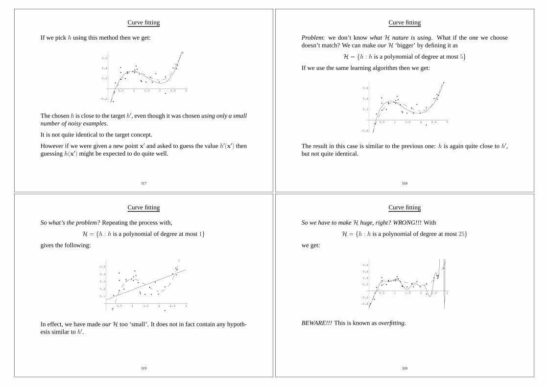
Curve fitting
If we pick h using this method then we get:
0.5 1 1.5 2 2.5 3
-0.2
0.2
0.4
0.6
The chosenh is close to the targeth′, even though it was chosenusing only a smallnumber of noisy examples.
It is not quite identical to the target concept.
However if we were given a new pointx′ and asked to guess the valueh′(x′) thenguessingh(x′) might be expected to do quite well.
317
Curve fitting
Problem: we don’t knowwhatH nature is using. What if the one we choosedoesn’t match? We can makeourH ‘bigger’ by defining it as
H = {h : h is a polynomial of degree at most5}If we use the same learning algorithm then we get:
0.5 1 1.5 2 2.5 3
-0.2
0.2
0.4
0.6
The result in this case is similar to the previous one:h is again quite close toh′,but not quite identical.
318
Curve fitting
So what’s the problem?Repeating the process with,
H = {h : h is a polynomial of degree at most1}gives the following:
0.5 1 1.5 2 2.5 3
0.1
0.2
0.3
0.4
0.5
In effect, we have madeourH too ‘small’. It does not in fact contain any hypoth-esis similar toh′.
319
Curve fitting
So we have to makeH huge, right? WRONG!!!With
H = {h : h is a polynomial of degree at most25}we get:
0.5 1 1.5 2 2.5 3
-0.4
-0.2
0.2
0.4
0.6
0.8
BEWARE!!!This is known asoverfitting.
320
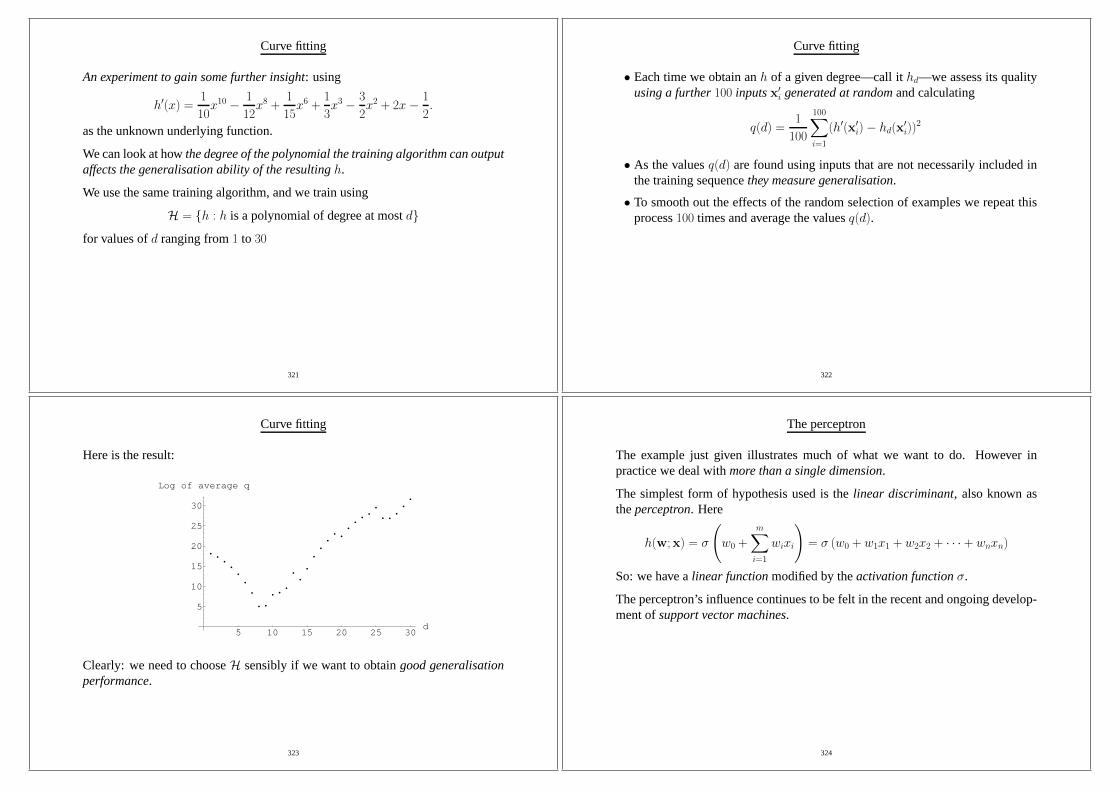
Curve fitting
An experiment to gain some further insight: using
h′(x) =1
10x10 − 1
12x8 +
1
15x6 +
1
3x3 − 3
2x2 + 2x− 1
2.
as the unknown underlying function.
We can look at howthe degree of the polynomial the training algorithm can outputaffects the generalisation ability of the resultingh.
We use the same training algorithm, and we train using
H = {h : h is a polynomial of degree at mostd}for values ofd ranging from1 to 30
321
Curve fitting
• Each time we obtain anh of a given degree—call ithd—we assess its qualityusing a further100 inputsx′i generated at randomand calculating
q(d) =1
100
100∑
i=1
(h′(x′i)− hd(x′i))
2
• As the valuesq(d) are found using inputs that are not necessarily included inthe training sequencethey measure generalisation.
• To smooth out the effects of the random selection of exampleswe repeat thisprocess100 times and average the valuesq(d).
322
Curve fitting
Here is the result:
5 10 15 20 25 30d
5
10
15
20
25
30
Log of average q
Clearly: we need to chooseH sensibly if we want to obtaingood generalisationperformance.
323
The perceptron
The example just given illustrates much of what we want to do.However inpractice we deal withmore than a single dimension.
The simplest form of hypothesis used is thelinear discriminant, also known astheperceptron. Here
h(w;x) = σ
(w0 +
m∑
i=1
wixi
)= σ (w0 + w1x1 + w2x2 + · · · + wnxn)
So: we have alinear functionmodified by theactivation functionσ.
The perceptron’s influence continues to be felt in the recentand ongoing develop-ment ofsupport vector machines.
324
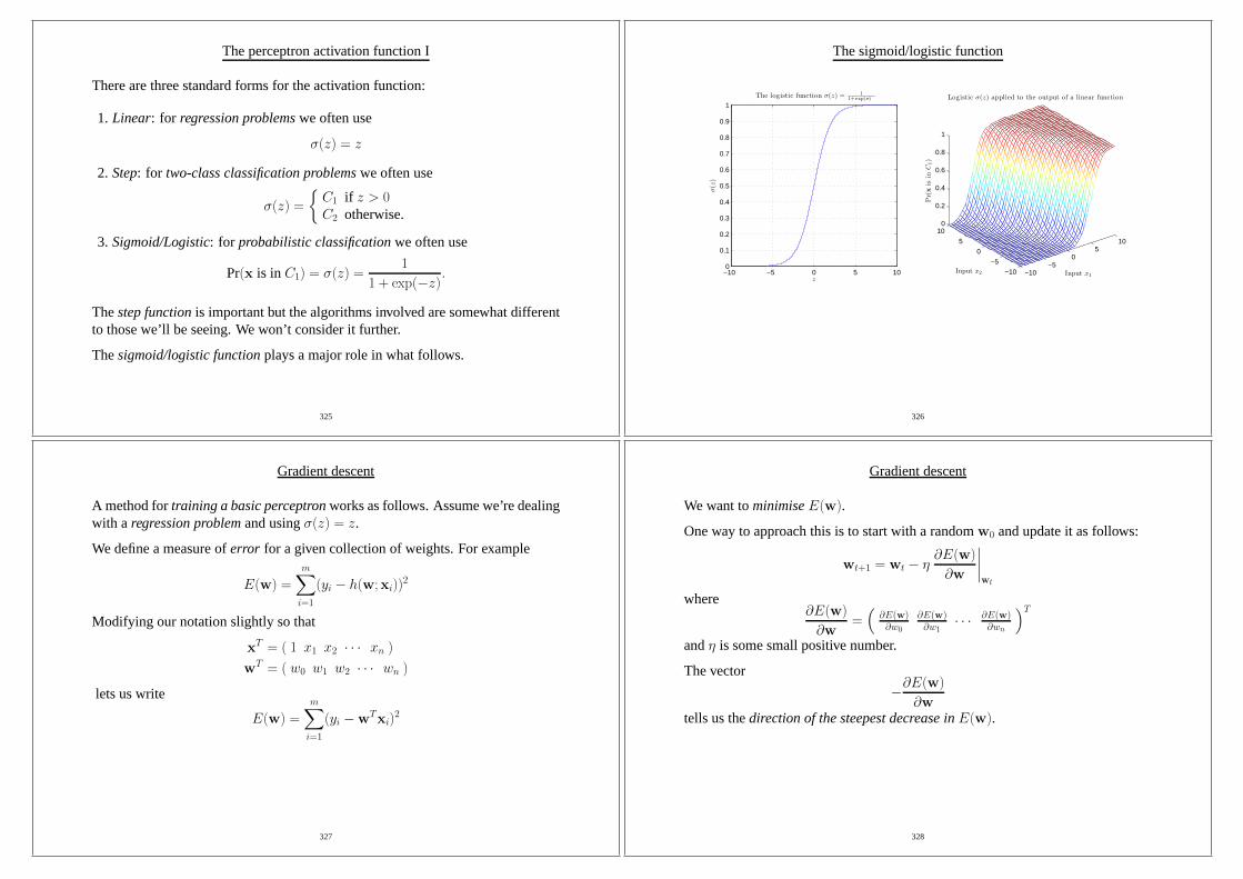
The perceptron activation function I
There are three standard forms for the activation function:
1. Linear: for regression problemswe often use
σ(z) = z
2. Step: for two-class classification problemswe often use
σ(z) =
{C1 if z > 0C2 otherwise.
3. Sigmoid/Logistic: for probabilistic classificationwe often use
Pr(x is inC1) = σ(z) =1
1 + exp(−z).
Thestep functionis important but the algorithms involved are somewhat differentto those we’ll be seeing. We won’t consider it further.
Thesigmoid/logistic functionplays a major role in what follows.
325
The sigmoid/logistic function
−10 −5 0 5 100
0.1
0.2
0.3
0.4
0.5
0.6
0.7
0.8
0.9
1The logistic function σ(z) = 1
1+exp(−z)
z
σ(z)
−10−5
05
10
−10
−5
0
5
100
0.2
0.4
0.6
0.8
1
Input x1
Logistic σ(z) applied to the output of a linear function
Input x2
Pr(xis
inC
1)
326
Gradient descent
A method fortraining a basic perceptronworks as follows. Assume we’re dealingwith a regression problemand usingσ(z) = z.
We define a measure oferror for a given collection of weights. For example
E(w) =m∑
i=1
(yi − h(w;xi))2
Modifying our notation slightly so that
xT = ( 1 x1 x2 · · · xn )
wT = ( w0 w1 w2 · · · wn )
lets us write
E(w) =
m∑
i=1
(yi −wTxi)2
327
Gradient descent
We want tominimiseE(w).
One way to approach this is to start with a randomw0 and update it as follows:
wt+1 = wt − η∂E(w)
∂w
∣∣∣∣wt
where∂E(w)
∂w=(
∂E(w)∂w0
∂E(w)∂w1
· · · ∂E(w)∂wn
)T
andη is some small positive number.
The vector
−∂E(w)
∂wtells us thedirection of the steepest decrease inE(w).
328
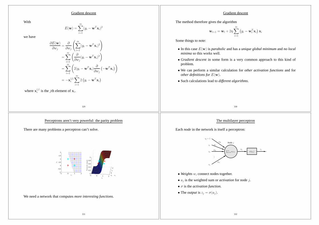
Gradient descent
With
E(w) =m∑
i=1
(yi −wTxi)2
we have
∂E(w)
∂wj=
∂
∂wj
(m∑
i=1
(yi −wTxi)2
)
=m∑
i=1
(∂
∂wj(yi −wTxi)
2
)
=m∑
i=1
(2(yi −wTxi)
∂
∂wj
(−wTxi
))
= −x(j)i
m∑
i=1
2(yi −wTxi
)
wherex(j)i is thejth element ofxi.
329
Gradient descent
The method therefore gives the algorithm
wt+1 = wt + 2ηm∑
i=1
(yi −wT
t xi
)xi
Some things to note:
• In this caseE(w) is parabolicand has aunique global minimumandno localminimaso this works well.
• Gradient descentin some form is a very common approach to this kind ofproblem.
• We can perform a similar calculation forother activation functionsand forother definitions forE(w).
• Such calculations lead todifferent algorithms.
330
Perceptrons aren’t very powerful: the parity problem
There are many problems a perceptron can’t solve.
−1 0 1 2−1
−0.5
0
0.5
1
1.5
2
x1
x2
−1 0 1 2 −1
0
1
2
0
0.2
0.4
0.6
0.8
1
x2
x1
Network
output
We need a network that computesmore interesting functions.
331
The multilayer perceptron
Eachnodein the network is itself a perceptron:
aj zjσ(aj)
w0
w1
w2
wn
...
Nodejz1
z2
zn
∑ni=0wizi
z0 = 1
• Weightswi connect nodes together.
• aj is the weighted sum oractivationfor nodej.
• σ is theactivation function.
• Theoutputis zj = σ(aj).
332
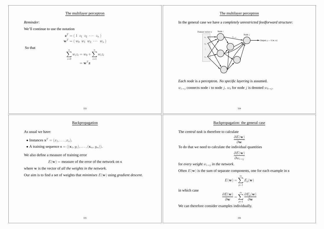
The multilayer perceptron
Reminder:
We’ll continue to use the notation
zT = ( 1 z1 z2 · · · zn )
wT = ( w0 w1 w2 · · · wn )
So thatn∑
i=0
wizi = w0 +n∑
i=1
wizi
= wTz
333
The multilayer perceptron
In the general case we have acompletely unrestricted feedforward structure:
Feature vectorx Nodei
Nodejwi→j
Outputy = h(w;x)
x1
x2
xn
...
Each nodeis a perceptron.No specific layeringis assumed.
wi→j connects nodei to nodej. w0 for nodej is denotedw0→j.
334
Backpropagation
As usual we have:
• InstancesxT = (x1, . . . , xn).
• A training sequences = ((x1, y1), . . . , (xm, ym)).
We also define a measure of training error
E(w) = measure of the error of the network ons
wherew is the vector ofall the weights in the network.
Our aim is to find a set of weights thatminimisesE(w) usinggradient descent.
335
Backpropagation: the general case
Thecentral taskis therefore to calculate∂E(w)
∂w
To do that we need to calculate the individual quantities
∂E(w)
∂wi→j
for every weightwi→j in the network.
OftenE(w) is the sum of separate components, one for each example ins
E(w) =m∑
p=1
Ep(w)
in which case∂E(w)
∂w=
m∑
p=1
∂Ep(w)
∂w
We can therefore consider examples individually.
336

Backpropagation: the general case
Place examplep at the input and calculateaj andzj for all nodesincluding theoutputy. This isforward propagation.
We have∂Ep(w)
∂wi→j=
∂Ep(w)
∂aj
∂aj∂wi→j
whereaj =∑
k wk→jzk.
Here the sum is overall the nodes connected to nodej. As
∂aj∂wi→j
=∂
∂wi→j
(∑
k
wk→jzk
)= zi
we can write∂Ep(w)
∂wi→j= δjzi
where we’ve defined
δj =∂Ep(w)
∂aj
337
Backpropagation: the general case
So we now need to calculate the values forδj...
Whenj is theoutput node—that is, the one producing the outputy = h(w;xp) ofthe network—this is easy aszj = y and
δj =∂Ep(w)
∂aj
=∂Ep(w)
∂y
∂y
∂aj
=∂Ep(w)
∂yσ′(aj)
using the fact thaty = σ(aj).
338
Backpropagation: the general case
The first term is in general easy to calculatefor a givenE as the error is generallyjust a measure of the distance betweeny and the label in the training sequence.
Example:whenEp(w) = (y − yp)
2
we have∂Ep(w)
∂y= 2(y − yp)
= 2(h(w;xp)− yp)
339
Backpropagation: the general case
Whenj is not an output nodewe need something different:
j
......
aj ak2
ak1
σ
σ
σ
σ
akq
k1
k2
kq
We’re interested in
δj =∂Ep(w)
∂ajAltering aj can affectseveral other nodesk1, k2, . . . , kq each of which can in turnaffectEp(w).
340

Backpropagation: the general case
j
......
aj ak2
ak1
σ
σ
σ
σ
akq
k1
k2
kq
We have
δj =∂Ep(w)
∂aj=
∑
k∈{k1,k2,...,kq}
∂Ep(w)
∂ak
∂ak∂aj
=∑
k∈{k1,k2,...,kq}δk∂ak∂aj
wherek1, k2, . . . , kq are the nodes to which nodej sends a connection.
341
Backpropagation: the general case
j
......
aj ak2
ak1
σ
σ
σ
σ
akq
k1
k2
kq
Because we know how to computeδj for the output nodewe canwork backwardscomputing furtherδ values.
We will always know all the valuesδk for nodes ahead of where we are.
Hence the termbackpropagation.
342
Backpropagation: the general case
j
......
aj ak2
ak1
σ
σ
σ
σ
akq
k1
k2
kq
∂ak∂aj
=∂
∂aj
(∑
i
wi→kσ(ai)
)= wj→kσ
′(aj)
andδj =
∑
k∈{k1,k2,...,kq}δkwj→kσ
′(aj) = σ′(aj)∑
k∈{k1,k2,...,kq}δkwj→k
343
Backpropagation: the general case
Summary: to calculate∂Ep(w)
∂w for thepth pattern:
1. Forward propagation: applyxp and calculate outputsetc for all the nodes inthe network.
2. Backpropagation 1: for theoutputnode
∂Ep(w)
∂wi→j= ziδj = ziσ
′(aj)∂Ep(w)
∂y
wherey = h(w;xp).
3. Backpropagation 2: For other nodes
∂Ep(w)
∂wi→j= ziσ
′(aj)∑
k
δkwj→k
where theδk were calculated at an earlier step.
344
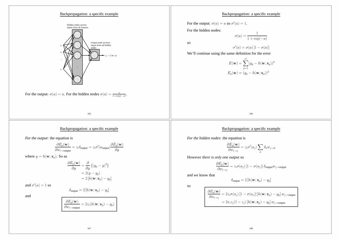
Backpropagation: a specific example
Hidden nodes receiveinputs from all features
Output node receivesinputs from all hiddennodes
y = h(w;x)
...
...
x2
x1
xn
For the output:σ(a) = a. For the hidden nodesσ(a) = 11+exp(−a).
345
Backpropagation: a specific example
For the output:σ(a) = a soσ′(a) = 1.
For the hidden nodes:σ(a) =
1
1 + exp(−a)so
σ′(a) = σ(a) [1− σ(a)]
We’ll continue using the same definition for the error
E(w) =m∑
p=1
(yp − h(w;xp))2
Ep(w) = (yp − h(w;xp))2
346
Backpropagation: a specific example
For the output: the equation is
∂Ep(w)
∂wi→output= ziδoutput= ziσ
′(aoutput)∂Ep(w)
∂y
wherey = h(w;xp). So as
∂Ep(w)
∂y=
∂
∂y
((yp − y)2
)
= 2(y − yp)
= 2 [h(w;xp)− yp]
andσ′(a) = 1 soδoutput= 2 [h(w;xp)− yp]
and∂Ep(w)
∂wi→output= 2zi(h(w;xp)− yp)
347
Backpropagation: a specific example
For the hidden nodes: the equation is
∂Ep(w)
∂wi→j= ziσ
′(aj)∑
k
δkwj→k
Howeverthere is only one outputso
∂Ep(w)
∂wi→j= ziσ(aj) [1− σ(aj)] δoutputwj→output
and we know thatδoutput= 2 [h(w;xp)− yp]
so∂Ep(w)
∂wi→j= 2ziσ(aj) [1− σ(aj)] [h(w;xp)− yp]wj→output
= 2xizj(1− zj) [h(w;xp)− yp]wj→output
348
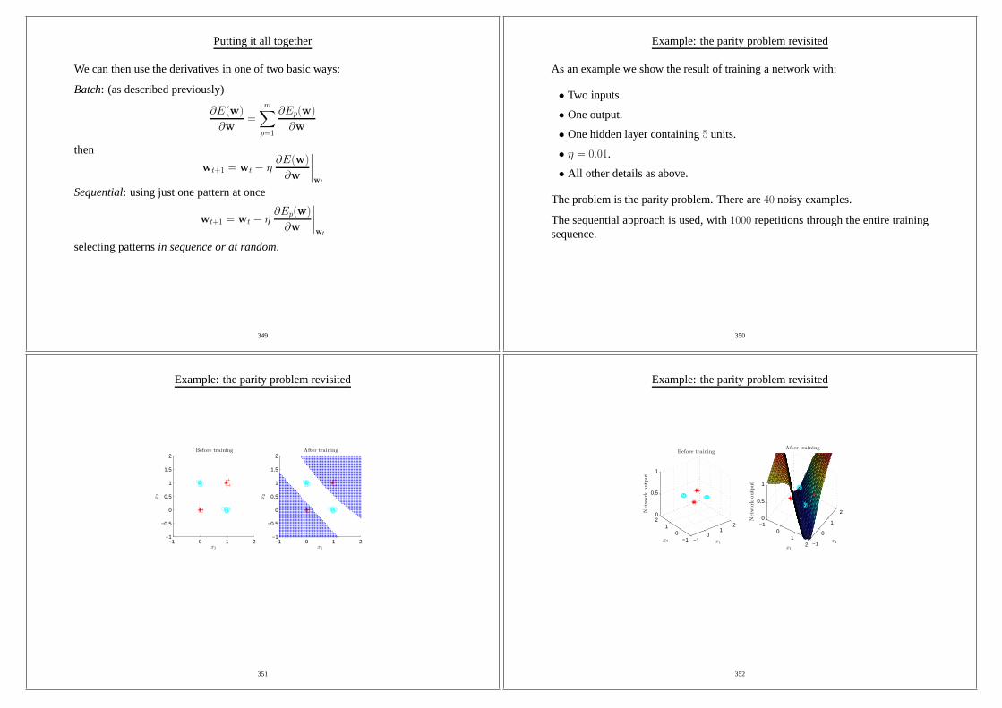
Putting it all together
We can then use the derivatives in one of two basic ways:
Batch: (as described previously)
∂E(w)
∂w=
m∑
p=1
∂Ep(w)
∂w
then
wt+1 = wt − η∂E(w)
∂w
∣∣∣∣wt
Sequential: using just one pattern at once
wt+1 = wt − η∂Ep(w)
∂w
∣∣∣∣wt
selecting patternsin sequence or at random.
349
Example: the parity problem revisited
As an example we show the result of training a network with:
• Two inputs.
• One output.
• One hidden layer containing5 units.
• η = 0.01.
• All other details as above.
The problem is the parity problem. There are40 noisy examples.
The sequential approach is used, with1000 repetitions through the entire trainingsequence.
350
Example: the parity problem revisited
−1 0 1 2−1
−0.5
0
0.5
1
1.5
2Before training
x1
x2
−1 0 1 2−1
−0.5
0
0.5
1
1.5
2After training
x1
x2
351
Example: the parity problem revisited
−10
12
−10
120
0.5
1
x1
Before training
x2
Network
output
−10
12 −1
0
1
20
0.5
1
x2
After training
x1
Network
output
352
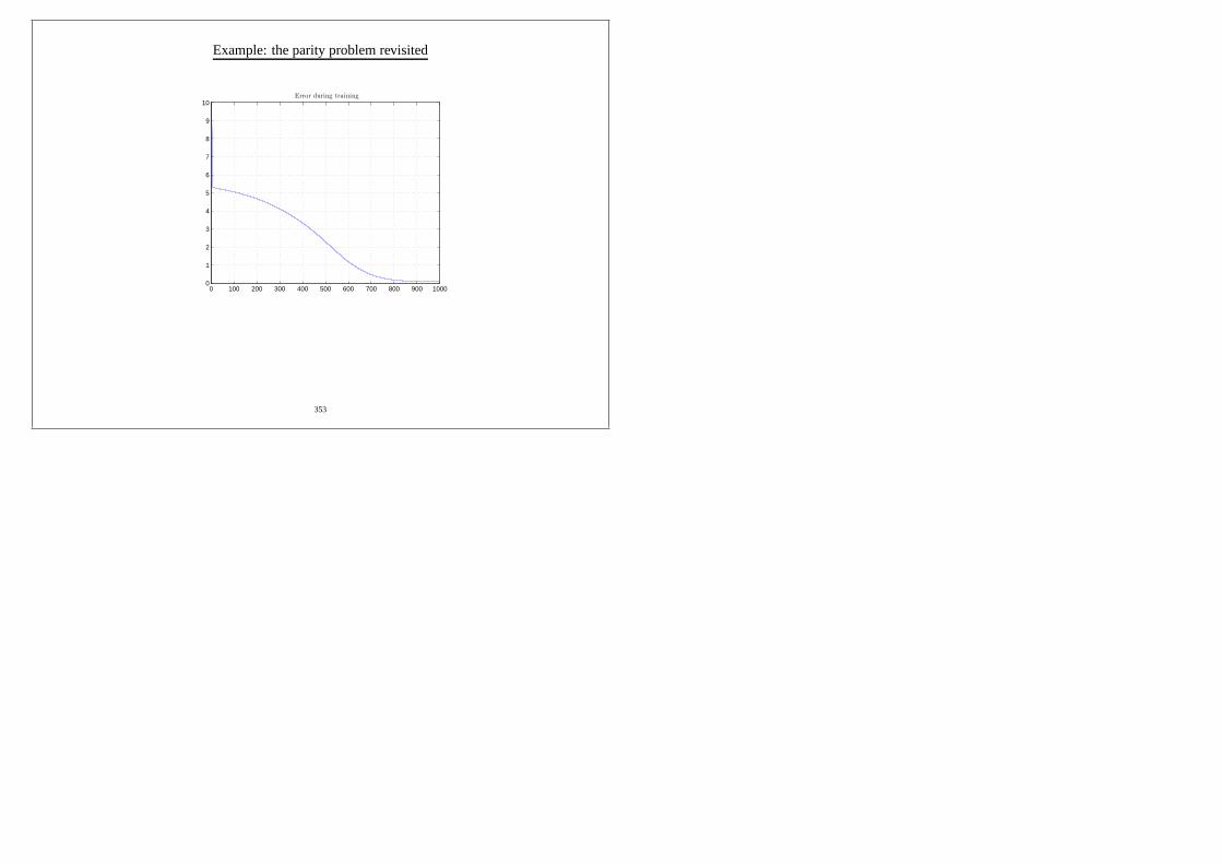
Example: the parity problem revisited
0 100 200 300 400 500 600 700 800 900 10000
1
2
3
4
5
6
7
8
9
10Error during training
353