Dynamism Diminished: The Role of

Housing Markets and Credit Conditions

Steven J. Davis and John Haltiwanger

Economics Working Paper 19102

HOOVER INSTITUTION

434 GALVEZ MALL

STANFORD UNIVERSITY

STANFORD, CA 94305-6010

January 10, 2019

The Great Recession and its aftermath saw the worst relative performance of young firms

in at least 35 years. More broadly, as we show, young-firm activity shares move strongly with

local economic conditions and local house price growth. In this light, we assess the effects of

housing prices and credit supply on young-firm activity. Our panel IV estimation on MSA-level

data yields large effects of local house price changes on local young-firm employment growth

and employment shares and a separate, smaller role for locally exogenous shifts in bank lending

supply. A novel test shows that house-price effects work through wealth, liquidity and collateral

effects on the propensity to start new firms and expand young ones. Aggregating local effects to

the national level, housing market ups and downs play a major role – as transmission channel

and driving force – in medium-run fluctuations in young-firm employment shares in recent

decades. The great housing bust after 2006 largely drove the cyclical collapse of young-firm

activity during the Great Recession, reinforced by a contraction in bank loan supply. As we also

show, when the young-firm activity share falls (rises), local employment shifts strongly away

from (towards) younger and less-educated workers.

The Hoover Institution Economics Working Paper Series allows authors to distribute research for

discussion and comment among other researchers. Working papers reflect the views of the

authors and not the views of the Hoover Institution.

William H. Abbot Distinguished Service Professor of International Business and Economics at the University of

Chicago Booth School of Business, Research Associate with the National Bureau of Economic Research, and Senior

Fellow at the Hoover Institution. Webpage: http://faculty.chicagobooth.edu/steven.davis/. Dudley and Louisa Dillard Professor of Economics and Distinguished University Professor of Economics at the

University of Maryland, College Park, and Research Associate with the National Bureau of Economic Research.

Webpage: http://econweb.umd.edu/~haltiwan/.

Dynamism Diminished: The Role of Housing Markets and Credit Conditions

Steven J. Davis and John Haltiwanger

Economics Working Paper 19102

January 10, 2019

JEL Codes: E2, E3, E5, G2, J2

Keywords: Young firms, business dynamism, housing market boom and bust, credit supply

shifts, Great Recession, employment fluctuations

Abstract:

The Great Recession and its aftermath saw the worst relative performance of young firms in at

least 35 years. More broadly, as we show, young-firm activity shares move strongly with local

economic conditions and local house price growth. In this light, we assess the effects of housing

prices and credit supply on young-firm activity. Our panel IV estimation on MSA-level data

yields large effects of local house price changes on local young-firm employment growth and

employment shares and a separate, smaller role for locally exogenous shifts in bank lending

supply. A novel test shows that house-price effects work through wealth, liquidity and collateral

effects on the propensity to start new firms and expand young ones. Aggregating local effects to

the national level, housing market ups and downs play a major role – as transmission channel

and driving force – in medium-run fluctuations in young-firm employment shares in recent

decades. The great housing bust after 2006 largely drove the cyclical collapse of young-firm

activity during the Great Recession, reinforced by a contraction in bank loan supply. As we also

show, when the young-firm activity share falls (rises), local employment shifts strongly away

from (towards) younger and less-educated workers.

Steve J. Davis

Hoover Institution, Stanford University

Booth School of Business, University of

Chicago

and NBER

http://faculty.chicagobooth.edu/steven.davis/

John Haltiwanger

University of Maryland,

College Park, MC 20742-7211

and NBER

http://econweb.umd.edu/~haltiwan/

Acknowledgments:

We thank Simon Gilchrist, John Robertson and participants in seminars and conferences at the

American Economic Association, Bank of Korea, Cambridge University, Congressional Budget

Office, Federal Reserve Bank of Atlanta, Goldman Sachs Global Markets Institute, Hoover

Institution, London School of Economics, National Bureau of Economic Research, National

University of Singapore, Stanford University and the University of Chicago for many helpful

comments. Diyue Guo and Laura Zhao provided superb research assistance. We gratefully

acknowledge financial support from the Goldman Sachs Global Markets Initiative and the Ewing

Marion Kauffman Foundation.

1

I. Introduction

Workers at young firms – less than 60 months since first paid employee – fell from 17.9

percent of private sector employees in 1987 to 9.1 percent in 2014 (Figure 1). This pronounced

shift away from young firms is part of a broader secular decline in business formation rates,

business volatility, the pace of job reallocation, and worker mobility rates in the United States.1

Overlaying these long-term developments, the growth rate of the young-firm activity share varies

cyclically, as seen in Figure 2. Each bar shows the average annual log change in the young-firm

employment share during the indicated cycle episode, deviated about the mean annual change

from 1981 to 2014. The young-firm share falls relative to trend in aggregate contractions and

rises or falls more slowly in expansions. Except for the early 2000s, the negative young-firm

fluctuation in contractions intensified over time, and the positive fluctuation in expansions

weakened. Indeed, the Great Recession and its aftermath involve the worst relative performance

for young firms in at least 35 years.

In light of these observations, we investigate three related questions: First, what is the

role of housing market developments, especially the massive boom and bust since the late 1990s,

in the fortunes of younger firms? Second, what is the role of credit market conditions? Third,

how do young-firm fortunes translate to labor market outcomes? To address these questions, we

exploit the abundant spatial and time-series variation in local housing market and credit

conditions in the United States. Our main goal is to better understand the cyclical and medium-

run fluctuations in the performance and activity shares of young firms.2 We seek to estimate the

causal effect of local house price changes on local young-firm activity and to develop evidence

on the channels through which housing prices affect young-firm activity. We also quantify the

role of house price changes and bank loan supply shocks in national and local fluctuations of

young-firm activity shares. Finally, we quantify the implications of young-firm activity shares

for employment outcomes by worker age, education and gender.

Section II describes our data sources for local young-firm activity measures, housing

prices, housing supply elasticities, credit supply shifts and cyclical conditions at the aggregate

1 These secular developments are well documented in recent work and the subject of active study. See Davis et al. (2007), Davis et al. (2010), Davis, Faberman and Haltiwanger (2012), Fujita (2012), Lazear and Spletzer (2012), Hyatt and Spletzer (2013), Davis and Haltiwanger (2014), Decker et al. (2014ab), Haltiwanger, Hathaway and Miranda (2014), Hathaway and Litan (2014ab), Karahan et al. (2015), Molloy et al. (2016) and Pugsley and Şahin (2018). 2 In contrast, recent work by Davis and Haltiwanger (2014) and Karahan et al. (2015), for example, consider forces behind the long-term shift away from younger firms.

2

and local levels. Section III first expands on our characterization of trend and cycle movements

in young-firm activity shares. At the national level, the Great Recession involved an historic

deterioration in young-firm performance (relative to a declining trend) on multiple margins,

including the firm startup rate and the growth rate of young relative to older firms. At the state

level, changes in young-firm employment shares covary strongly and positively with local cycle

conditions and with the growth rate of local house prices.

Section IV implements two IV estimation approaches to identify the causal effect of local

house price changes on local young-firm activity shares.3 Our first approach exploits national

housing boom and bust episodes that differentially affect MSA-level house prices due to

differences in local housing supply elasticities. To obtain instruments that isolate arguably

exogenous variation in local house price movements, we interact period effects (boom and bust)

with the Saiz (2010) housing supply elasticity measure. The identification idea is that a common

shock to local housing demand generates cross-MSA differences in local house price movements

due to exogenous spatial differences in housing supply elasticities. This approach follows the

same identification strategy as the highly influential work of Mian and Sufi (2009, 2011, 2014),

but we focus on a different outcome variable (young-firm activity shares) and consider additional

controls to address various threats to identification. In our second IV approach, we instrument

local house price changes using the interaction between local housing supply elasticity and local

cyclical indicators.

Our two IV approaches exploit different sources of data variation, but they yield similar

estimates for the effect of local house price changes on young-firm activity shares. Both

approaches address (serious) concerns about measurement error in local house price data.

Beyond that, each approach offers certain advantages and disadvantages. In its focus on national

boom and bust episodes, the first IV approach facilitates comparisons to previous research. By

encompassing a much longer time period and eleven times as many observations, the second

approach readily accommodates the inclusion of local loan supply shocks.

We supplement our second IV approach by building on Greenstone, Mas and Ngyugen

(2015) to isolate exogenous MSA-level shifts in the supply of bank lending to small (and young)

3 Our focus on activity shares differs from previous work on how local house prices affect the demand for local non-traded goods and services (e.g., Mian and Sufi, 2011), local self-employment and small-firm employment (e.g., Adelino et al., 2015), and the local pace of job creation and destruction at young firms (e.g., Mehrotra and Sergeyev, 2016). In particular, shocks that affect the level of local economic activity – but not its distribution between young and mature firms – have no effect on our main outcome measures.

3

firms.4 The idea here is that large banks differ in their financial fortunes, geographic footprints and

propensities to lend to smaller and younger firms. When a national bank pulls back from lending

to smaller and younger firms in a given MSA for reasons other than local economic conditions, it

produces an exogenous drop in loan supply to young firms in the MSA. Consistent with this view,

we find that “small” business bank loan supply shocks have statistically significant effects on

young-firm activity shares, and that these shocks have noteworthy effects on young-firm activity

shares in certain episodes, particularly the Great Recession.

We also show that “small” business loan supply shocks have weaker effects on small firms

than young ones. Siemer (2018) reaches the same conclusion using different data and an empirical

design that exploits industry differences in the role of external financing. In addition, we find

weaker effects of housing prices on small firms than young ones. These findings reflect the

heterogeneous character of the small-firm population. The bulk of small-firm employment resides

in firms that are mature, relatively stable, and have little need or desire for credit-fueled expansion.

In contrast, young firms are much more volatile and highly prone to up-or-out growth dynamics.5

Most young firms are also small. Thus, shocks to the supply of “small” business bank lending have

much stronger effects on activity in young firms than in the average small firm.

As we discuss in Section V, housing market conditions can affect young firms and the

local economy through a variety of wealth, liquidity, collateral, credit supply and consumption

demand channels. That discussion leads us to data and empirical designs that help disentangle

these channels. Since many studies find large effects of housing price changes on consumption

expenditures, we test whether they affect local economies only through consumption demand.

Our test of this view is new and conceptually simple: If house price changes work entirely

through consumption demand channels, the local industry growth rate response should be

invariant to the age structure of firms in the local industry. A natural alternative to this age-

invariance hypothesis says that the local industry response rises with its young-firm activity

share due to wealth, collateral, and liquidity effects of house prices on the propensity to start a

new business or expand a young one. We find overwhelming statistical evidence against the age-

4 Other related work with a focus on the Great Recession period includes Chodorow-Reich (2014), Burcu et al. (2015), Huang and Stephens (2015) and Siemer (2018). Our empirical approach to identifying bank loan supply shocks is closest to that of Greenstone et al. (2015). 5 For evidence that young age is much more indicative of high growth propensity, while small size is not (conditional on age), see Section 4.2 in Davis and Haltiwanger (1999) and Haltiwanger, Jarmin and Miranda (2013). For evidence on the prevalence of up or out behavior among younger businesses, see Davis et al. (2009) and Haltiwanger et al. (2016).

4

invariance hypothesis. The departures from age invariance fit the alternative view and involve

large effects on the distribution of employment growth across MSA-industry cells in periods

with large housing price movements. In a dynamic extension, we also find that the positive

effect of local house prices changes on local industry growth rates is both larger and more

persistent in MSA-industry cells with a larger share of young-firm activity.

To quantify the role of housing market developments, Section VI combines local house

price changes with IV estimates of their causal effect to obtain implied paths for local young-firm

activity shares. We then aggregate to the national level and ask how well the results account for

the episode-by-episode cycle movements in Figure 2 and analogous year-by-year changes. By

design, our quantification exercise captures the effects of exogenous house price changes and the

role of house prices in transmitting shocks that originate elsewhere. The exercise also incorporates

a separate role for exogenous bank loan supply shifts. The quantification results imply that housing

market ups and downs are a major driver of medium-run fluctuations in young-firm activity shares,

especially since the late 1990s. The great housing bust after 2006 largely drove the collapse of

young-firm activity shares (relative to a declining trend) during the Great Recession, reinforced by

the effects of a contraction in bank loan supply. Shifts in the supply of bank lending also played a

material role in certain other episodes – contributing, for example, to the mild cyclical contraction

in young-firm activity in the early 2000s (Figure 2). A rebound in bank lending from 2010 to 2014

prevented an even larger decline in the young-firm employment share.

Section VII investigates how the fortunes of young firms play out in the labor market. We

show that changes in local young-firm activity disproportionately load onto the employment of

younger and less-educated workers for both men and women. The dramatic drop in young-firm

activity shares during the Great Recession helps explain why younger and less-educated workers

fared even more poorly in the labor market than other demographic groups.

II. Data Sources

a. Young-Firm Activity Measures

Fort et al. (2013) and Davis and Haltiwanger (2014) show that spatial and industry

variation in job flows, worker flows, and growth rate differentials by firm size and age provide

much scope for analysis and identification. We also exploit data sets that offer variation by firm

age, firm size, industry and local area (State or MSA). Our outcome measures derive from

administrative records that cover all firms with paid employees. A key advantage of the resulting

5

activity measures is that they are not subject to missing observations or sampling variability,

even within narrow geographic and industry cells.

Our analysis of young-firm activity relies heavily on two Census Bureau statistical products:

Business Dynamic Statistics (BDS) and Quarterly Workforce Indicators (QWI). The BDS

includes employment statistics by firm size, firm age, state, MSA and industry tabulated from

micro data in the Longitudinal Business Database (LBD).6 The LBD covers the universe of firms

and establishments in the nonfarm business sector with at least one paid employee. Employee

counts pertain to the payroll period covering the 12th of March in each year from 1976 to 2014.

The LBD includes the location of each establishment and, hence, the distribution of each firm’s

employment across states and MSAs. While firm characteristics reflect the national firm, the

BDS state (MSA) activity measures cover all establishments operating in the state (MSA) for the

industry, firm size or firm age group.

For our purposes, it is essential to have a suitable measure of firm age and to consistently

track young-firm activity over time. Firm age in the BDS reflects the age of its oldest

establishment when the firm first became a legal entity. In turn, establishment age equals the

number of years since operations began (as indicated by one or more paid employees) in the

establishment’s current narrowly defined industry. For a startup business comprised of all new

establishments, firm age is initially set to zero. For firms newly created from one or more

existing establishments through a merger, spinoff or corporate reorganization, firm age is

initially set to the age of its oldest establishment. From that point forward, the firm ages naturally

as long as it exists. Simple ownership changes do not trigger a change in firm age, and the BDS

concept of business startups reflects new firms with only age-zero establishments. These

features of the BDS are a major strength, as they ensure that our young-firm activity measures

and their evolution are not distorted by firm restructurings and ownership changes.

For simplicity and brevity, our analysis focuses on two age groups: “young” firms less

than five years old (fewer than 60 months), and “mature” firms that are at least five years old.

Using these definitions, the BDS enables us to track young- and mature-firm activity measures at

the national and state levels in a consistent manner from 1981 to 2014 and from 1992 to 2014 at

the MSA level. The BDS reports employment and firm counts as of March in the indicated year

and March-to-March changes and growth rates. Appendix A provides more information about

the level, change and growth rate statistics in the BDS and how we exploit the data.

6 The BDS is a public use database at www.census.gov/ces/dataproducts/bds/index.html.

6

The BDS does not simultaneously classify young-firm activity measures by state (or

MSA) and industry. To overcome this limitation, we turn to the QWI in Section V when we

investigate the channels through which house price changes affect young-firm and industry

activity shares. We use the QWI to track young-firm employment at the MSA-industry-age level

for more than 30 states from 1999 to 2015. The firm age concept in the QWI follows the BDS

exactly. We also exploit the QWI to investigate how young-firm activity shares vary with

employment outcomes by gender, age and education in MSA and MSA-industry level data.

b. Local Housing Price and Supply Elasticity Measures

We measure house price changes using data at the state and MSA levels from the Federal

Housing Finance Agency (FHFA). These data are available for the entire 1981-2014 period

considered in our analysis. As explained below, we seek to isolate local house price movements

that are exogenous with respect to local young-firm activity shares by interacting other variables

with the Saiz (2010) measure of the local housing supply elasticity. His measure, available at the

MSA level, reflects a careful effort to quantify supply elasticities based on detailed studies of

local zoning, regulatory and natural topographic and geophysical barriers to residential housing

construction. Saiz produces housing supply elasticities for 248 MSAs. For 15 of these MSAs, we

cannot produce all regressors in our empirical specifications on a balanced-panel basis. Thus, we

typically report results for samples that contain 233 MSAs, roughly three times as many as in

Mian and Sufi (2011).

c. Bank Lending Measures

We follow Greenstone, Mas and Ngyugen (2015) (hereafter GMN) in using data on small

business loan activity that banks file in compliance with the Community Re-Investment Act of

1996 (CRA). The CRA requires banks with assets greater than 1 billion to report annually on

small business loans at the county level. We aggregate these CRA data to the MSA level. Like

GMN, we consider the volume of loans to businesses with less than $1 million in gross revenue.

We build on the GMN approach to construct local “small” business loan supply shocks using a

modified Bartik-like approach, as detailed in Section V below. Although the CRA data explicitly

specify loans to small business, we think there is considerable overlap between credit supply

shifts for small business lending and credit supply shifts for young business lending. Our

empirical results strongly support that view.

When integrating data across sources, we pay careful attention to the timing of the

observations. BDS employment data reflect the payroll period covering the 12th day of March in

each calendar year. We measure employment changes and changes in all other variables over the

7

same March-to-March intervals. It is straightforward to align the timing for most of our

variables, because they are available on a monthly or quarterly basis. The annual CRA data are

an exception. Appendix C details how we construct our CRA-based measures.

d. Local and National Cycle Indicators and Other Variables

We supplement our young-firm activity measures with local and national business cycle

indicators. At the state and MSA level, we use unemployment rates from the BLS Local Area

Unemployment Statistics (LAUS) program, which draws on data from the Current Population

Survey, Current Employment Statistics, claims for unemployment insurance benefits and other

sources. We have consistent measures of unemployment rates at the state level from 1980 to

2014 and at the MSA level from 1990 to 2014. We use real GDP growth rates as a national

business cycle indicator. We obtain annual county-level population data from the Census Bureau,

which we map to MSA as explained in Appendix A. Finally, we rely on the Quarterly Census of

Employment and Wages (QCEW) at the national and MSA-industry level (2-digit NAICS) to

construct additional controls and instruments for local demand shifts.

III. Secular, Cyclical and Spatial Patterns in Young-Firm Activity

a. Aggregate Measures of Young-Firm Activity

The patterns depicted in Figures 1 and 2 reflect changes along several margins at young and

mature firms. To see this point, write the change from t-1 to t in young-firm employment as

!"#$% − !"'(#$% = [!"+ + ∑ (!"# −/#0( !"'(#'()] − !"'(/ ≡ 4!5"#$% − !"'(/ (1)

where !"#$% is employment in young firms (age<5) in year t, !"+ is employment in startup firms

(age=0) in t, and !"# is employment in firms of age a in t. This accounting identity says that the

young-firm employment change equals the net change among firms that remain young, inclusive

of new employment at startup firms, minus employment at firms that age out of the young group.

Similarly, the employment change from t-1 to t among mature firms is the net change among the

already mature as of t-1 plus employment at firms that age into the mature group in t. A parallel

set of accounting relationships holds for the numbers of young and mature firms.

We express young-firm employment as a share of total private-sector employment. Thus,

Figure 1 plots the evolution of !"#$%/!", where !" is the count of all paid employees in the

nonfarm private sector in March of year t. Figure 2 plots the average annual value of

78(!"#$%/!") − 78(!"'(#$%/!"'() for each cycle episode, deviated about its mean value from 1981

8

to 2014. Appendix B presents additional evidence on the secular and cyclical behavior of young-

firm activity measures, which we summarize here. Appendix Figure B1 shows a strong secular

decline in the firm startup rate since the mid 1980s, a further large drop in the Great Recession,

and little recovery afterwards. The firm exit rate moves counter cyclically with little or no trend.7

The net entry rate of firms actually turned negative in the Great Recession for the first time since

at least 1981, and it remains near zero more recently. These developments translate into a

pronounced drop in the share of firms with paid employees that are less than five years old –

from nearly 45 percent in 1981 to 28 percent in 2014 (Figure B2).

Figure B3 reports net growth rates for young-firm and mature-firm employment,

inclusive of entry and exit for each age group.8 For changes from t-1 to t, the BDS classifies

establishments into firm age groups based on age of parent firm at t. Young firms exhibit much

higher net growth rates than mature firms. This pattern underscores the importance of young

firms in the job creation process, as highlighted in Haltiwanger et al. (2013). However, young

firms exhibit larger growth rate declines in downturns, especially so in the Great Recession. In

fact, the net employment growth rate of young firms plummeted from 24 percent in 2006 to 8

percent in 2009, a dramatic negative swing of 16 percentage points. By way of comparison, the

net employment growth rate of mature firms fell from zero in 2006 to minus 6 percent in 2009.

Appendix B also presents analogs to Figure 2 for other young-firm activity measures.

Figure B4 shows that the early 1980s and the Great Recession saw especially large declines

relative to trend in the young-firm share of firms with paid employees. Figure B5 shows that the

net employment growth rate of young firms saw especially large declines relative to mature firms

in the 1990-91 downturn and in the Great Recession. It’s worth stressing that the Great

Recession involved an historic deterioration in young-firm performance for all of the activity

measures we consider. In what follows, we focus on the young-firm employment share, but

Figures B1-B5 make clear that secular declines and procyclical movements in young-firm

performance are present on several margins.

7 The BDS measure of firm exit rates reflect legal entities that shut down all establishments. Like the startup rate, the BDS exit rate concept is designed to abstract from firm ownership changes and M&A activity. 8 The BDS follows Davis, Haltiwanger and Schuh (1996) in calculating group-level growth rates as the employment weighted average of establishment-level growth rates in the group, where each establishment’s growth rate is measured as its change from t-1 to t divided by the simple average of its employment in t-1 and t.

9

b. State-Level Fluctuations in Young-Firm Employment Shares

Our empirical study exploits spatial and time variation to investigate the influence of

credit conditions and housing markets on young-firm activity. To help motivate this approach,

Figure 3A presents a scatter plot of log differences in young-firm employment shares (vertical

axis) against changes in the unemployment rate (horizontal axis) at the state-year level for the

period from 1981 to 2014. There is much state-level time series variation in these measures,

which we will use in our econometric investigation. An increase in the state-level unemployment

rate of one percentage point is associated with a 1.77 log point drop in the state’s young-firm

employment share. Figure 3B shows the contemporaneous relationship between log differences

in the young-firm employment share (vertical axis) and log differences in real housing prices at

the state-year level from 1981 to 2014. Greater house price appreciation in a state tends to

coincide with a larger rise (or smaller fall) in its young-firm employment share. A real house

price gain of 10 log points in a state is associated with an increase in its young-firm employment

share of 3 log points. The t-statistic for this relationship is about 15.9 Appendix Figures B6 and

B7 show that greater house price appreciation in a state also coincides with a larger rise (or

smaller fall) in the young-firm share of all firms with paid employees and in the firm startup rate.

Figure 3B and the related results in Figures B6 and B7 might appear at odds with results

in Hurst and Lusardi (2004). Using data from the Panel Study of Income Dynamics (PSID) and

regional house price variation from 1985 to 1988, they test whether households in Census

regions with strong house price gains were as unlikely to start a business as households in other

regions. They do not reject this hypothesis. Restricting our state-level panel data to the 1985-

1988 period in Hurst and Lusardi, and rerunning our Figure 3B regression, yields an estimated

coefficient of 0.29 (0.06). So different sample periods do not explain our different results.

Instead, we think the different results reflect important conceptual and measurement differences

between our study and theirs. First, business starts in the PSID include those with no employees,

while our measures consider only firms with paid employees. Davis et. al. (2009) show that non-

employer businesses are much more numerous than employer businesses, but most non-employer

businesses are very small, contribute little to aggregate economic activity, and are unlikely to

9 Figure 3b reveals a few large outliers in the log changes of young-firm shares. The estimated relationship is robust to winsorizing the log differences at the 99.75 and the 0.25 percentiles (one quarter of one percent). The estimated slope coefficient is 0.29 (0.02) with the winsorized data compared to 0.30 (0.02) in Figure 3b.

10

ever hire a worker. Second, our use of administrative data sources yields much more precise

estimates of young-firm activity in narrower geographic areas.

Figures 3A and 3B also indicate that the empirical relationships among changes in

unemployment rates, house prices and young-firm employment shares are approximately (log)

linear in our data. We stick to linear specifications in the econometric results reported below. In

unreported results, we find little evidence of departures from linearity.

In summary, Figures 3A and 3B tell us that stronger state-level economic conditions and

rising house prices involve an increase in the state’s share of economic activity accounted for by

young firms. Of course, these empirical relationships do not tell us why young-firm activity

shares covary strongly with local conditions, but they suggest the possibility that housing market

developments have important causal effects on young-firm activity shares. Hurst and Stafford

(2004), Mian and Sufi (2011), Mian, Sufi and Trebbi (2015) and Agarwal et al. (2015), among

others, find evidence that house price appreciation stimulates household spending and local

economic activity more generally. As noted, our focus is on the effects of house price movements

on young-firm activity shares in the local economy.

IV. Local Effects of Housing Prices and Loan Supply on Young-Firm Activity

a. Overview of Estimation and Identification

We implement two instrumental variables (IV) estimation strategies to identify the causal

effects of local house price changes on local young-firm activity shares. Specifically, we

construct instruments for housing price changes by interacting local housing supply elasticities

from Saiz (2010) with time-period effects (first approach) or with time-varying local economic

conditions (second approach). Our first approach uses the same identification strategy as Mian

and Sufi (2011) but differs in its focus on young-firm activity shares and in our use of panel data

to control for unobserved factors that affect local MSA trends. Our second approach covers a

much longer period and facilitates the inclusion of loan supply shocks.

b. Boom-Bust Panel Regressions – IV Approach 1

Our first IV approach uses 466 observations on annual average log changes in MSA-level

data – 233 boom changes from 2002 to 2006 and 233 bust changes from 2007 to 2010. We use

these data to estimate the following statistical model:

:;< = ∑ =<><< + ∑ =;>;; + ?@A;< + B;< (2) (Second stage)

@A;< = ∑ C;>;; + ∑ C<><< + ∑ ><D;E F<< + G;< (3) (First stage)

11

where :;< is the log change in the young-firm employment share for MSA m and period s, @A;<

is the contemporaneous log change in the MSA’s house price index, >< is a dummy for period s,

>; is dummy for MSA m, D;is a cubic polynomial in the Saiz housing supply elasticity, and =H

andCH are coefficients on dummy variables. The chief parameter of interest is ?, the response of

the change in the local young-firm employment share to the local house price change.

To identify ? we rely on the exclusion restrictions,E(><D;E , B;<) = 0, which says that

><D;E influences young-firm employment shares only through house price growth, conditional on

period and MSA effects. Stacking boom and bust episodes lets us control for MSA-specific

trends in the 2000s, addressing concerns that these trends reflect other factors that happen to

correlate with local housing supply elasticities, as argued by Davidoff (2016). We consider other

threats to identification shortly.

Figure 4 shows the MSA-level changes in young-firm employment shares and house

prices that we use to estimate (2) and (3). Housing prices rose across MSAs during the boom

from 2002 to 2006, and they fell in the vast majority of MSAs during the bust from 2007 to

2010. Both periods exhibit enormous local variation and a strong positive relationship across

MSAs between changes in housing prices and young-firm employment shares. Other periods

show smaller movements, which makes them less useful under IV approach 1.

Table 1 reports regression results for specification (2) fit to the MSA-level data. We find

a positive, statistically significant effect of local housing price growth on local young-firm

activity shares. According to the IV estimates in Column (4), which control for common period

effects and MSA-specific trends during the 2000s, an increase in local real housing prices of 10

log points per year yields a gain of 1.94 log points per year in the local young-firm employment

share. IV estimates for ? are somewhat larger than the corresponding OLS estimates, in line

with the view that measurement error in the local housing price indices produces some

attenuation under OLS. F-tests show a very strong first stage, with test statistics well above 10.

As seen in Figure 5, the IV-estimated relationship in Table 1 is very similar in the boom and bust

periods, and it is not driven by a few outliers.

We think the IV estimation strategy and Column (4) specification in Table 1 yields a

plausible estimate for the causal effect of local house price changes on the local young-firm

employment share. The specification controls for unobserved factors that drive MSA-specific

trends in young-firm activity shares during the 2000 and that also correlate with the Saiz housing

supply elasticity across MSAs. The specification also controls for common period effects, and it

12

deals with measurement error in the housing price indices. We don’t think reverse causality is a

concern, given our choice of dependent variable in (2). That is, we do not think exogenous shifts

in the local young-firm share of activity drive changes in local house price growth.

A more serious concern is that (2) and (3) may not adequately control for local shocks

that affect local house price growth and our second-stage outcome measure, :;<. Omitted

variables with these properties can produce a failure of our key identifying assumption,

!(><D;E , B;<) = 0. To see this point, suppose the true specification is:

:;< = ∑ =<><< + ∑ =;>;; + ?@A;< + O;<E P+B;< (2') (Second stage)

@A;< = ∑ C;>;; + ∑ C<><< + ∑ ><D;E γ<< + O;<E R + G;< (3') (First stage)

where O;<is a vector of local shocks that affects young-firm activity shares and local house

prices. Suppose further that !(><D;E , O;<) ≠ 0, i.e., the local shocks O;< are also correlated with

our instrument. These circumstances violate our exclusion restriction, !(><D;E , B;<) = 0, in the

estimated system (2) and (3), yielding a bias of unknown direction in the estimate of ?. 10 A

solution is to instead estimate the system (2') and (3') with controls for O;<.

Motivated by this type of identification threat, we now consider three additional controls.

First, we include a local cycle control: the average annualized change in the MSA-level

unemployment rate during the period. Second, we control for a local demand shifter that varies

by MSA and period, which we construct as (the lagged MSA-level industry employment share)

X (the current-period national industry employment growth) summed over all 2-digit NAICS

industries.11 Finally, we control for the average annualized growth rate in the MSA-level

population during the period, using data from the Bureau of the Census.

Table 2 reports regression results for (2'). We again find a strong positive impact of

local housing price growth on young firm activity shares for the IV results. Conditioning on all

three additional controls in Column (4), an increase in local real housing prices of 10 log points

per year raises the local young-firm employment share by 1.61 log points per year.12 This effect

10 As one example of an omitted variable that causes a downward bias in the estimate of ?, suppose that local housing prices rise with the entry (exit) of local establishments operated by mature national firms. This type of entry (exit) by mature firms also causes a mechanical decrease (increase) in the young-firm employment share. 11 We use annual QCEW data to construct this Bartik-type measure, averaging over years for each MSA within the boom and bust periods, respectively. Results are similar using 4-digit industry data, but there is much cell-level data suppression at that level of disaggregation. 12 Because of the dotcom bust, San Francisco stands out as an MSA with a large drop in the

13

is statistically significant at the 5 percent level, and an F-test again provides strong evidence

against the hypothesis of weak instruments.

c. Annual Panel Regressions – IV Approach 2

Our second IV approach uses annual data and a different source of variation to construct

instruments for MSA-level house-price changes. Specifically, we estimate the following model:

:;" = ∑ =">"" + ∑ =;>;; + ?@A;" + VW:W;" + O;"E P+B;" (4) (Second stage)

@A;" = ∑ C;>;; + ∑ C">"< + W:W;"D;E F + XW:W;" + O;"E R + G;" (5) (First stage)

where :;" is the log change from year t-1 to t in the young-firm share for MSA m, W:W;" is the

contemporaneous change in the MSA-level unemployment rate, and O;" is an additional set of

controls that vary at the MSA-year level. As before, we consider MSA fixed effects and

common period effects as controls. We again use the local housing supply elasticity to construct

instruments, but we now interact it with a local cycle measure rather a common period effect.

Hence, IV approach 2 relies on a different source of variation than IV approach 1. Approach 2

also exploits data for a much longer time span, yielding eleven times as many observations.

The exclusion restriction is now !(W:W;"D;E , B;") = 0; i.e., the interaction between the

local cycle and local supply elasticity affects :;" only through its effect on local house price

growth, @A;", conditional on controls. The motivation for IV 2 applied to the system (4) and (5)

is similar to that of IV 1 applied to the earlier system. Specifically, the IV approach addresses

concerns about measurement error, and it allows us to isolate aspects of local house price

changes that are plausibly exogenous with respect to changes in local young-firm activity shares.

For the same reasons as before, we do not think reverse causality is a serious concern. And as

before, we address concerns related to omitted variables by including multiple controls.

Table 3 reports estimates for ?, the chief parameter of interest in (4). The sample contains

the same 233 MSAs as before but now covers the period from 1992 to 2014. Qualitatively, the

Table 3 results are the same as those in Tables 1 and 2, but the IV estimates of ? are 50-100

percent larger in Table 3. (However, the precision of the estimates makes it hard to draw strong

conclusions in this regard.) According to Column (4), which entails the fullest set of controls, an

annual increase in local real housing prices of 10 log points raises the local young-firm

young-firm employment share from 2002 to 2006, even as local housing prices appreciated. In unreported results that exclude data for San Francisco, the estimate of ? corresponding to Column (4) in Table 2 is 2.03, notably larger than the full-sample estimate.

14

employment share by 3.0 log points. The gaps between OLS and IV estimates of ? are much

greater in Table 3 than in Tables 1 and 2, which makes good sense given concerns about

measurement error in the local housing price indices. In particular, local house price changes are

greater during the boom and bust than in other periods. Thus, the signal-to-noise ratio in the

housing price indices is larger in the boom-bust sample than in the full 1992-2014 sample. As a

consequence, attenuation bias under OLS is greater in Table 3 than in Tables 1 and 2.

d. Adding Small Business Lending Shocks under IV Approach 2

We now extend (4) and (5) to incorporate a role for “small” business loan supply shocks

as potential drivers of young-firm activity shares. As discussed in Section V, multiple sources of

credit supply shifts can affect young-firm activity. For the moment, we aim to estimate the role

of shifts in bank loan supply to small and young firms due to forces that are exogenous to local

economic activity. We follow the approach of GMN (2015), who exploit the fact that national

and regional banks differ in their financial fortunes and their geographic footprints. To see the

basic idea, suppose bank B with a large local footprint reduces its lending to small and young

firms nationally for reasons unrelated to local conditions. Bank B’s pullback in local lending to

young firms reduces their credit access, assuming credit supply is less than perfectly elastic.

To operationalize this idea and construct local loan supply shocks, we use CRA data on

the volume of individual bank lending to small businesses in each MSA.13 For every pair of

consecutive years, we first fit the following regression by weighted least squares:

Y;Z" = [\];" + ^_8 Z̀" + BHZ" (6)

where Y;Z"is the growth rate in the volume of real small business loans by bank holding

company j in MSA m from t-1 to t, and we weight by the bank’s volume of small business loans

in MSA m in t-1. The MSA effects control for local conditions, and the Bank effects capture the

national growth of small business lending by the bank holding company (hereafter, “bank”).

Next, to estimate the locally exogenous component of the growth rate in small business

bank lending to MSA m, we construct a Bartik-like measure given by:

\^a;" = ∑ b;Z"'(Z ^_8`cZ" (7)

where b;Z,"'( is bank j’s share of small business lending in MSA m at t-1. SBL captures cross-

MSA variation in small business lending by the national banks that differ in their fortunes and in

13 See Appendix C for more information about the CRA data and how we use them.

15

the geographic footprints of their small business lending activity. We treat this measure as

exogenous to local young-firm employment shares.

Incorporating small business loan supply shocks, our statistical model becomes

:;" = ∑ =">"" + ∑ =;>;; + ?@A;" + VW:W;" + d\^a;" + O;"E P+B;" (8)

@A;" = ∑ C;>;; + ∑ C">"< + W:W;"D;E F + XW:W;" + e\^a;" + O;"E R + G;" (9)

Because our SBL data run only from 1999 to 2014, we lose the ability to control for year effects

in an unrestricted manner while retaining enough power to recover precise estimates for the key

parameters. Thus, we drop the year effects and instead introduce a quadratic polynomial in

national GDP growth rates in the X vector.

Table 4 reports OLS and IV estimates of the key parameters in (8). We find positive,

statistically significant effects of local bank loan supply shocks on local young-firm activity

shares. An increase in the loan supply shock of 10 log points raises the local young-firm

employment share by 0.2 to 0.24 log points in the IV specifications. The estimated effects of

local housing price changes in Table 4 are very similar to results in Table 3, despite the shorter

sample period and inclusion of loan supply shocks. The evidence that bank loan supply shocks

matter for young-firm activity shares is weaker than the evidence that housing price growth

matters. As we will see below, the bank loan supply shocks also play a much smaller role in

accounting for the medium- and short-run fluctuations in young-firm activity shares.

e. Results for the Employment Growth Rate as Dependent Variable

By treating the young-firm employment share as the dependent variable, the

specifications in Tables 1-4 control for omitted variables that have equiproportional effects on

the activity levels of young and mature firms. This specification feature is attractive from an

identification standpoint, but we are also interested in effects on employment growth. To that

end, Table 5 reconsiders the statistical model (8) and (9) but treats MSA-level growth rates in the

employment of young and mature firms as dependent variables. According to the IV results in

Panel A, an increase in local housing prices of 10 log points raises local young-firm employment

by 3.1 to 3.3 log points. Panel B, in contrast, shows a much smaller effect on mature-firm

employment that is statistically insignificant when including our full battery of controls. Loan

supply shocks also have much larger effects on young-firm than mature-firm employment. In

short, Table 5 says that house-price changes and loan supply shocks generate much large

percentage changes in the activity levels of young firms as compared to mature ones.

16

f. Small vs. Young-Firm Effects

Thus far, we have focused on how housing market conditions and bank loan supply affect

young-firm activity. Young firms are also small (Davis et al., 2007 and Haltiwanger, Jarmin and

Miranda, 2013). Moreover, as discussed in Gertler and Gilchrist (1994) and Fort et al. (2013),

firm size often serves as a proxy for access to credit markets. A natural question then is whether

our main findings hold for small firms as well as young ones. The short answer is no: Our main

findings do not hold up if we consider small-firm activity shares as the outcome of interest,

although some aspects of our results hold in weaker form. Appendix B provides detailed backing

for this claim. Here, we summarize a few key points and explain why young-firm activity shares

are more responsive than small-firm shares.

For present purposes, we define small firms as those with fewer than 50 paid employees.

Using this threshold, the small-firm share of private-sector employees fell from 32 percent in

1981 to 27 percent in 2014. This aspect of small-firm behavior mirrors, in muted form, the

secular fall in young-firm shares. However, unlike the pattern documented in Figure 2, the small-

firm employment share moves counter cyclically (Appendix Figure B.8). An important reason

for this dynamic pattern is that many firms slip below the small-large threshold in contractions

and rise above it during expansions (Davis, Haltiwanger and Schuh, 1996).

In Table B.1, we compare the results of estimating (8) with the small-firm share as the

dependent variable to the results for the young-firm share. Whether we run OLS or IV 2, the

estimated effects of local housing price growth are about three-to-four times greater on young-

firm shares than on small-firm shares. The same pattern holds for the estimated effects of small

business bank loan supply shocks. That is, “small” business bank loan supply shocks have larger

estimated effects on young-firm shares than on small-firm shares.

Given the threshold-crossing issue, we also conduct the small-versus-young comparison

using a different dependent variable. Accordingly, Table B.2 reports the results of estimating (8)

for the growth rate differential between small firms and large ones, where we classify each firm

into a given size bin for t-1 and t based on its size in t. This approach follows Davis and

Haltiwanger (1999) and Fort et al. (2013). Table B.2 also reports results of estimating (8) for the

growth rate differential between young and mature firms. Local house price changes have similar

effects on the local young-mature and small-large employment growth differentials. We also find

strong statistical evidence that local small business loan supply shocks affect young-firm shares

but no statistically discernable effect on local small-firm shares.

17

We interpret these results as evidence that young firms in particular, rather than small firms,

are especially sensitive to credit availability. As discussed in Gertler and Gilchrist (1994), the

informational frictions that raise external financing costs pertain to young firms more than small

ones. Young firms are also more dynamic, and more likely to bump up against credit restrictions

that constrain their growth. Most mature small firms, in contrast, have little prospect for rapid

growth regardless of credit availability.

V. Transmission Channels

a. From House Prices and Credit Supply to Young-Firm Activity

Local housing market conditions can affect young-firm activity and the local economy

through a variety of wealth, liquidity, collateral, credit supply, and consumption demand

channels. Independent of local housing market conditions, other local and national

developments can shift the supply of credit that young firms tap to finance their activities.

Empirically, Robb and Robinson (2012) show that young firms finance their activities using

home equity loans, personal loans, bank loans, and personal wealth.

Much previous research finds a positive empirical relationship between personal wealth

and the propensity to start or own a business. Examples include Evans and Jovanovic (1989),

Holtz-Eakin et al. (1994), Gentry and Hubbard (2004) and Hurst and Lusardi (2004). Empirical

studies that specifically consider the impact of changes in home equity values on the propensity

to become self-employed or otherwise start a business include Black et al. (1996), Fan and White

(2003), Fairlie and Krashinsky (2012), Adelino et al. (2015), Schmalz, Sraer and Thesmar

(2015), Kerr, Kerr and Nanda (2015) and Harding and Rosenthal (2017). Jensen et al. (2014)

exploit high-quality Danish micro data and a legal change in 1992 that, for the first time, allowed

home equity to serve as collateral in bank loans to finance consumption expenditures or business

investment. This exogenous relaxation of collateral constraints led to an increase in new

business formation, more so for households that experienced larger increases in usable collateral.

We turn now to a discussion of several channels through which house price changes and

credit supply shifts can affect business startup rates and young-firm activity shares.

Wealth Effects on Business Formation and Expansion

A classic paper by Khilstrom and Laffont (1979) models the choice between operating a

risky firm and working for a riskless wage in general equilibrium. Individuals in their model

differ in absolute risk aversion levels. The least risk-averse individuals become entrepreneurs,

and the rest choose to be workers. Under certain regularity conditions, greater risk tolerances in

18

the population lead to a greater number of entrepreneurs in equilibrium and higher wages. While

Khilstrom and Laffont do not model the determinants of risk aversion, a time-honored view

holds that absolute risk tolerance rises with wealth. Guiso and Paiella (2008) provide evidence.

Thus, by raising wealth levels, a local house-price boom increases risk tolerances among local

homeowners and thereby stimulates new firm formation.

If existing young-firm owners face a similar tradeoff between less risky (stay small) and

more risky (become larger) undertakings, wealth gains among existing young-firm owners lead

to increases in their business activity levels. Kihlstrom and Laffont describe conditions that

ensure more risk-tolerant entrepreneurs run larger firms. Thus, insofar as many young-firm

owners also own homes, a housing price boom (bust) will lead to an expansion (contraction) in

young-firm activity levels. Of course, this mechanism also applies to homeowners who own

mature firms. We think local young-firm activity levels are likely to exhibit a larger proportional

response to local house price growth for two reasons: young-firm owners are more likely to own

a home in the same area as their businesses, and home equity is likely to form a larger share of

overall wealth for young-firm owners as compared to mature-firm owners.

In short, the entrepreneurial choice model of Khilstrom and Laffont, plus standard views

about wealth and risk tolerance, imply that local house price booms (busts) cause an upturn

(downturn) in the local firm startup rate and in the local young-firm activity share. The latter

implication also rests on an auxiliary assumption of greater proportional responses to local house

price changes among young-firm owners.

Wealth effects on young-firm activity shares can also arise for other reasons. Hurst and

Pugsley (2017) focus on the non-pecuniary benefits of business ownership such as “wanting to

be my own boss” and “wanting to pursue my passion.” They model the non-pecuniary benefits of

business ownership as separable from the utility of other consumption goods. Thus, as wealth

rises and the marginal utility of other consumption falls, households become more inclined to

indulge their tastes for business ownership. Effectively, owning a business is a normal good, the

demand for which rises with wealth. If local house price gains (losses) lead to higher (lower)

expenditures on other consumption goods, then housing booms (busts) nudge additional

households into (out of) business ownership.

The Hurst-Pugsley mechanism provides a clear transmission channel from greater

housing wealth to greater self-employment. The implications for startups with paid employees

and young-firm employment shares are less clear. “Wanting to be my own boss” is a motive for

self-employment but does not require a business with paid employees. However, owning a

19

business with paid employees indulges a taste for bossing others. So, depending on their precise

nature, non-pecuniary benefits of owning a business may or may not translate into a wealth effect

on the formation of new businesses with paid employees or on young-firm employment shares.

Liquidity and Collateral Effects

Evans and Jovanovic (1989) focus on differences in entrepreneurial ability and liquidity

constraints as the key factors determining which individuals start a business. A large follow-on

literature concludes that relaxing credit constraints at the household level leads to greater self-

employment and more business startups. Examples include most of the studies cited above on

the impact of changes in home equity values on the propensity to become self-employed or start

a business. The common theme in these studies is that households can tap home equity gains to

relax liquidity constraints, increasing their ability to finance new and young businesses.

Moreover, banks that make loans to these households (or their businesses) collateralized by

home equity become more willing to extend credit as house price gains yield greater home

values. Of course, home equity collateral can facilitate the expansion of mature firms as well. As

in our discussion of wealth effects, there are good reasons to anticipate proportionally greater

effects of local house price gains on local young-firm activity relative to mature-firm activity.

Credit Supply Shifts

New and young firms often rely on the owner’s personal wealth to finance business

activities, but their very newness implies little accumulation of business equity. And few young

firms are well positioned to raise equity or debt capital from external investors. For these

reasons, new and young businesses are likely to be especially sensitive to credit supply shifts that

involve bank loans to businesses and business owners (perhaps secured by housing collateral),

personal credit cards, and other sources of credit that young-firm owners and young firms,

especially, tap to finance their business activities.

It is helpful to distinguish among various reasons for local credit supply shifts. First, local

economic fortunes affect the lending capacity of local banks. Insofar as new and younger firms

are relatively dependent on credit from local banks, shocks to the lending capacity of local banks

have a greater effect on young firms. The same point holds for local housing developments that

affect the lending capacity of local banks. When local banks suffer losses due to a bust in the

local housing market, their lending capacities diminish and the credit supply effects are likely to

weigh more heavily on younger firms. In other words, the effect of house price movements on

young-firm activity shares works partly through the capacity of local lenders to extend credit to

young firms and their owners. Other things equal, this impact of local housing market

20

developments on local young-firm activity shares – working through the credit supply channel –

is smaller when local banks are less important as a source of credit to the local economy.

Second, both local and national banks are likely to see local housing prices as indicators

of (future) local business conditions, affecting their willingness to lend. To be sure, this link

between house prices and bank lending reflects a perceived shift in business fundamentals rather

than a locally exogenous shift in credit supply. Nevertheless, the impact of such a shift in bank

willingness to lend to local businesses or their owners falls more heavily on young firms for

reasons we have discussed.

Empirically, local house price changes covary positively with changes in the volume of

bank loans to local small (and presumably younger) businesses, as shown in Figure 6. To

construct the figure, we first regress annual log changes in real housing prices and the real

volume of bank loans to small businesses at the state-year level on state and year fixed effects

and annual changes in the state-level unemployment rate. We then plot the loan volume change

residuals against the house price change residuals. Even after sweeping out state, year and local

cycle effects, there is a strong relationship between house prices and bank loan volume to small

businesses. The empirical elasticity of local small business loan volume growth with respect to

local house price growth is 0.58 with a t-statistic of about 7.

Third, local credit supply can shift due to factors that are exogenous to local economic

conditions and to local businesses. For example, when a national bank pulls back from lending to

smaller and younger firms in a given MSA for reasons other than local economic conditions, it

produces a locally exogenous drop in loan supply to young firms in the MSA. Our empirical

investigation in Section IV exploits this type of exogenous variation in bank loan supply to

estimate the causal effects of local credit supply shifts on local young-firm activity shares.

Consumption Demand Channel

Recall from Section III that changes in young-firm activity shares covary strongly with

business cycle conditions in national and state-level data. These patterns suggest that demands

for the goods and services supplied by young firms are more income elastic than the demands for

mature-firm products. If so, then local young-firm demands are also likely to be more elastic

with respect to wealth shifts induced by local housing market ups and downs. In principle, this

type of non-uniform consumption demand shift could fully explain the response of young-firm

activity shares to local house price movements that we find in Section IV. We turn next to a

novel test of the proposition that local house-price changes affect the local economy – including

local young-firm activity shares – only through consumption demand channels.

21

b. Local Industry Responses to Local House Price Changes: A Test

We now investigate whether and how the local industry growth response to local house

price changes depends on the local industry’s firm-age structure of employment. If house prices

work entirely through consumption demand channels, the local industry response will not depend

on its firm-age structure. This invariance proposition is our null hypothesis in the test below. In

contrast, if the wealth, liquidity, collateral and credit supply effects described above are at work,

the local industry growth response to local house price changes will rise with the local industry’s

young-firm activity share. This proposition is our alternative hypothesis in the test below.

We implement this test using annual QWI data on employment and the firm-age structure

of employment at the industry-by-MSA level from 1999 to 2015. QWI data have three great

advantages for this purpose. First, the four-way sorting of employment into firm

age/industry/MSA/year cells affords a powerful test and a precise characterization of any

departures from age invariance. Second, the QWI derives from mandatory tax filings for

businesses with paid employees. As a result, we are not confronted by the small samples,

reporting errors and non-responses that present difficult challenges in survey data. Third, the

QWI data cover a time period with huge local house prices changes, which lets us precisely

estimate the effects of interest.

We use the following 14 industry groups for each MSA: Construction (NAICS 23),

Manufacturing (31-33), Wholesale Trade (42), Retail Trade (44-45), Transportation and

Warehousing (48-49), Information (51), Finance and Insurance (52), Real Estate and Rental and

Leasing (53), Professional, Scientific and Technical Services (54), Management of Companies

and Enterprises (55), Administrative and Support and Waste Management and Remediation

Services (56), Health Care and Social Assistance (62), Arts, Entertainment and Recreation (71)

and Accommodation and Food Services (72). We omit Agricultural Services (11), Mining (21)

and Utilities (22), because they have positive employment in few MSAs. We omit Educational

Services (61) and Other Services (81) because of QWI coverage limitations.14

Now consider the regression specification,

fgZ;" = _ + h(W:W;" + hi@A;" + hj:kl8Y\ℎZ;,"'(

+n ∙ @A;" × :kl8Y\ℎZ;,"'( + q" + q; + qZ + BZ;" (10)

14 The QWI mostly covers non-profits and religious organizations in NAICS 61 and 81. QWI local employment growth in these two industries has a weak relationship to local cyclical variables, including house price changes.

22

where fgZ;" is the log employment change from year t-1 to t for industry j in MSA m,W:W;" is

a control for local economic conditions in MSA m in year t,@A;" is the log house price change

from year t-1 to t in MSA m, and :kl8Y\ℎZ;,"'( is the lagged young-firm employment share in

industry j and MSA m. The f terms denote fixed effects, and BZ;" is an error term. As before, we

use the change in the local unemployment rate from year t-1 to t as our W:W;" control. The chief

coefficient of interest is c, which tells us how the local industry-level response to local house

price changes varies with the (lagged) young-firm share of employment in the local industry.

Formally, the null hypothesis is n = 0, and the alternative is n > 0.

Table 6, Panel A reports results for (10) fit to QWI data by OLS and IV. The data

resoundingly reject the age-invariance proposition: n̂ = 0.81 in Column (1), and a one-sided test

of the null hypothesis yields a t-statistic of nearly 14. In words, the local industry response to

higher local house prices rises with the local industry’s young-firm employment share. This

result supports the view that local house prices affect the local economy at least partly through

wealth, liquidity, collateral and credit supply effects on the propensity to start a new business or

expand a young one. Put differently, consumption demand effects do not fully explain the impact

of local house prices on local employment.

The regression controls in column (1) guard against a spurious rejection of the age-

invariance proposition due to certain unmeasured factors. For example, easier credit conditions at

the national level may drive a more rapid appreciation of home prices and a credit-fueled

increase in young-firm employment shares at the same time. Conversely, tighter credit conditions

may slow or reverse home price appreciation and constrict young-firm employment shares. The

year effects control for this source of covariation between local house price changes and young-

firm activity shares. Similarly, the inclusion of MSA effects control for the tendency of cities

with higher population growth to experience greater home price appreciation and stronger gains

in young-firm employment shares.

Column (2) of Panel A in Table 6 includes a full set of MSA-year effects as controls,

with little effect on the coefficient of interest. This result tells us that unmeasured sources of city-

level growth rate fluctuations (which might cause systematic co-movements between local

changes in home prices and young-firm shares) cannot account for our rejection of the age-

invariance proposition. Column (3) adds industry-year effects, and again we reject the age-

invariance proposition. Finally, column (4) uses our IV2 strategy and, once again, the data

23

resoundingly reject the null in favor of the alternative. In short, the statistical evidence against

the age-invariance proposition is overwhelming and unlikely to be caused by omitted factors.

How large are the departures from age invariance? To address this question, we compute

the regression-implied response differential between the 90th and 10th percentiles of the young-

firm employment shares across MSA-industry cells. We evaluate this response differential at

various points in the distribution of local house price changes. To be precise, we calculate

guvwk8vu_yzqq = n̂{:kl8Y\ℎ|+'(+}@A(w), (11)

where n̂ is the estimated coefficient on the interaction term in regression (10), :kl8Y\ℎ|+'(+ is

the 90-10 differential in young-firm employment shares across local industries, and @A(w) is the

pth percentile of annual log changes in MSA-level home prices.

Table 7 quantifies the departures from age invariance. Panels A and B report inputs to

(11), and panel C implements the calculation using n̂ = 0.813 from Column (1) in Table 6, Panel

A. Evaluating at the 90th percentile of the MSA-level house price change in the Boom, the

employment growth response differential is 2.2 log points per year between local industries at

the 90th and 10th percentiles of the young-firm employment share distribution. The cumulative

response differential is 9.4 log points over the Boom Period as a whole from 2002 to 2006.

Evaluating at the 10th percentile of the MSA-level house price distribution in the Bust, the

response differential is -2.3 log points per year. These are large departures from age invariance.

Of course, when MSA-level house price changes are small, the induced response differential

between industries with high and low young-firm employment shares is small as well.

c. Hysteresis Effects and the Firm-Age Structure of Employment

Lastly, we extend specification (10) to include the lagged main effect for local housing

price changes and its interaction with the lagged young-firm employment share in the local

industry. For brevity, Panel B in Table 6 reports only the coefficients on the interaction effects in

this dynamic extension to (10); the other coefficients are similar to the ones in Panel A.

This dynamic extension yields two additional results: First, the local industry response to

an increase in local house prices now rises even more steeply with the local industry’s young-

firm share. For example, the immediate interaction effect is 1.295 in column (1) of Panel B, as

compared to 0.813 for the static specification reported in Panel A. Second, the dynamic

extension implies an amplification of the immediate interaction effect in the following year. To

see this point, note first that local housing price changes are highly persistent, with an AR1

24

coefficient of 0.73 (s.e. of 0.012) when controlling for MSA fixed effects. Combining this AR

coefficient with the results in Column (1) of Panel B, the average net interaction effect one year

after a local housing price increase is (1.295 ∗ 0.73) − 0.696 = 0.249. Thus, the effect of a

local housing price increase on local industry employment growth rises in period t with the local

industry’s young-firm share, and it rises even further in period t+1. In terms of local industry

employment levels, these results imply powerful hysteresis effects of local housing price changes

that vary with the firm-age structure of employment in the local industry.

VI. Assessing Effects on Aggregate Young-Firm Activity Shares

We now quantify the contribution of house price movements and exogenous loan supply

shifts to aggregate fluctuations in young-firm activity shares. We first apply our estimation

results to obtain implied paths for changes in local young-firm employment shares. Then we

aggregate to the national level using local-area employment shares.

When we quantify the effects of house price changes on local young-firm activity shares, we

multiply the IV estimate for ? by the actual changes in local housing prices. This approach

captures the full effect of housing prices on local young-firm activity shares, including their role

as a transmission channel through which other shocks drive housing price changes. We think this

full effect is the most interesting quantity. Isolating the role of local house-price changes as an

exogenous driver of young-firm activity shares would require additional assumptions to

disentangle the exogenous and endogenous components of house-price movements.15

There are three other important points to keep in mind about our aggregate quantification

exercise. First, and most obviously, the exercise proceeds under an assumption of correctly

identified casual effects at the local level.

Second, local causal effects need not aggregate as simply as we presume. For example, a

drop in young-firm activity in one area could raise young-firm activity in other areas through a

spatial substitution response in product and factor markets. Conversely, young-firm activity in

one area could have positive spillover effects on young-firm activity in other areas. As a separate

point that cuts in the same direction, entrepreneurs can own houses outside the area where they

operate young firms. This fact raises the possibility that local house price changes in one area

15 The first stage in the IV estimation identifies exogenous house-price movements, but there’s no reason to think it captures all, or even most, of the movements in housing prices that are exogenous with respect to local young-firm employment shares.

25

directly affect young-firm activity shares in other areas, a possibility neglected by our statistical

models. The net effect of these spatial forces is unclear to us, even as to direction, but we see no

reason to think they are large relative to the effects captured by our models. Still, we recognize

that our neglect of spatial spillover and spatial equilibrium considerations may bias our

assessment of aggregate implications.

Third, recall that our econometric specifications include period fixed effects as controls.

These controls condition out the common response across local areas to economy-wide

developments. For example, if a national housing bust leads to a broad constriction in credit

supply – and that constriction has disproportionately large effects on the employment growth of

new and young firms – then the housing bust lowers the national young-firm employment share

in a manner not reflected in our aggregate quantification exercise. The same point holds in

reverse for a national housing boom. The upshot is that our quantification exercise may

understate the full effect of the national housing boom and bust on fluctuations in young-firm

employment shares, because it neglects the general equilibrium effects of national housing

booms and busts that affect credit availability in a similar way across local areas.

Figure 7 implements our quantification exercise using the IV2 estimates for ? from the

rightmost column in Table 3. The solid bars in Panel A reproduce Figure 2. The striped bars

show the model-implied paths for aggregate changes in young-firm employment shares by cycle

episode. We treat states as local areas for this purpose, so we can push the quantification exercise

back to the early 1980s. State-level data also let us cover the entire United States, including rural

areas.16 As in Figure 2, we express both actual and model-implied paths as deviations from the

sample trend.17 Panel B implements the quantification exercise on a year-by-year basis.

The results in Figure 7 show that housing market ups and downs are a major force behind

cyclical and medium-run fluctuations in young-firm activity shares. According to Panel A, 61

percent of the sharp decline in the young-firm employment share during the Great Recession

reflects the effects of housing price declines. Housing price movements also play an important

role in several other cycle episodes. As seen in Panel B, the cumulative effect of housing price

16 Re-estimating our statistical model on state-level instead of MSA-level data yields estimates for ? similar to the ones reported in Table 3, but the point estimates are less precise. 17 The growth in our national housing price index is nearly identical to the employment-weighted growth of our state-level housing price indices. Thus, given the linearity of our statistical model, multiplying the log change in the national housing price index by the estimated value for ? yields nearly identical results to the ones displayed in Figure 8.

26

gains from 1997 to 2006 raised the national young-firm employment share by 11 log points. That

stimulus to young-firm activity offset one-half of the trend decline in young-firm employment

during this period. However, this boost to the young-firm employment share during the national

housing boom was mostly undone from 2008 to 2014 as a result of the national housing bust.

Figure 8 repeats the quantification exercise using our extended statistical model with

bank loan supply shocks. The role of housing price movements implied by the extended model is

very similar to before. However, the extended model also implies a distinct role for small

business bank loan supply shocks as driver of fluctuations in young-firm shares. Panel A in

Figure 8 shows that a contraction in small business lending during the Great Recession further

depressed the aggregate young-firm employment share. The joint contribution of the housing

bust and the pullback in small business bank lending accounts for 85 percent of the huge drop in

the young-firm employment share (relative to trend) during the 2008-2010 period. 65 percent of

the 85 percent is due to housing prices and 20 percent due to small business lending shocks.

Shocks to the supply of small business lending also have material effects on the young-

firm share in a few other cycle episodes. During the 2001-03 period, both housing price changes

and small business lending shocks worked to offset other forces that reduced the young-firm

employment share. These other forces probably include the fallout from the dotcom bust and the

recession in the early 2000s. During the recovery after the Great Recession period, housing

prices and small business lending worked in opposite directions. Housing price developments

continued to act as a drag on young-firm employment shares, while small business lending

provided a modest boost.

Panel B in Figure 8 shows the net contribution of housing prices and small business bank

lending shocks to year-by-year fluctuations in the young-firm employment shares from 1999 to

2014. This figure shows that our extended statistical model explains a good deal of the aggregate

fluctuations in young-firm shares since the late 1990s. But there are also notable fluctuations in

young-firm shares not explained by our model. In particular, the model says little about the

sizable moves in the late 1990s and early 2000s, which may reflect the dotcom boom and bust.

VII. Implications for the Labor Market

Prior research offers ample grounds for hypothesizing that the fortunes of young firms have

important and uneven effects in the labor market. Young firms account for a disproportionate

share of newly created job positions (Davis and Haltiwanger, 1992 and 1999), which makes them

highly active in the search, matching and hiring process. Ouimet and Zarutskie (2014) show that

27

young firms disproportionately employ young workers. They point to several reasons: skill-

demand differences between young and mature firms, positive assortative matching, and a higher

propensity for young firms and young workers to engage in search and matching. Haltiwanger et

al. (2018) and Haltiwanger, Hyatt, and McEntarfer (2018) show that young firms facilitate

movements up the job ladder by younger and less-educated workers. Young firms are important

for these workers as initial labor market entry ports and as re-entry ports when they get knocked

off the job ladder in contractions.

These findings prompt us to investigate the relationship between young-firm activity and the

distribution of employment by worker age, education and gender. Table 8 first confirms that

young firms disproportionately employ young workers. It also shows they disproportionately

employ less educated workers. This employment pattern leaves younger and less-educated

workers more exposed to the cyclical fortunes of young firms. We directly confirm this inference

in Figure B.11, which shows changes in the aggregate share of employment at young firms by

demographic group and cycle episode.

To delve more deeply into the empirical relationship between young-firm activity and the

demographic structure of employment, we fit regressions of the form

∆\;á" = [\];á + Xá∆à;" + O" P

á + B;á" (12)

to annual MSA-level observations for each demographic group, where ∆\;á"is the change from

t-1 to t in group g’s share of employment in MSA m, ∆à;" is the contemporaneous change in the

MSA’s share of employment at young firms, [\];á is a set of MSA fixed effects, and O" is a

quadratic polynomial in the national GDP growth rate. The chief parameters of interest in this

specification are the Xá coefficients, one for each demographic group.

Recall that we use QWI statistics to compute ƈ;". While these statistics derive from the

universe of administrative records for tax-paying firms, they are subject to noise infusion to

protect the confidentiality of employers (Abowd et al., 2009). The noise infusion process yields

random measurement errors in our ƈ;" observations, generating an attenuation bias in the OLS

estimator of the Xá coefficients. To address this issue, our preferred estimator for Xá relies on a

two-stage approach. The first stage instruments for ƈ;" using contemporaneous values of the

MSA-level change in the unemployment rate, log change in the real MSA-level housing price

index, and MSA-level small business loan supply shocks. This two-stage approach resolves the

28

attenuation bias.18 It also serves to isolate local economic forces that involve systematic co-

movements in local young-firm activity, as shown by our results in Sections III and IV.

Table 9 reports estimates for Xá in Columns (1) to (4). In line with our remarks about the

noise-infused nature of QWI data, the two-stage estimates are much larger in magnitude than the

corresponding OLS estimates. The two-stage estimates provide powerful evidence that changes

in the fortunes of young firms involve large shifts in the demographic structure of employment.

For men, a one percentage-point gain in the young-firm share of MSA employment involves a

0.36 percentage point gain in the local share of workers who are 25-44 and a 0.54 drop in the

share who are 45-54. For women, a gain in the local young-firm employment share involves an

even larger shift from older to younger workers. The table also reveals large shifts in the

educational mix of local employment with changes in the MSA’s young-firm share. For both

men and women, a gain in the young-firm share of local employment involves a shift in local

employment from more- to less-educated workers.

Columns (5) and (6) report two-stage estimation results for regressions at the MSA-industry

level. In addition to the controls in the MSA-level regressions, the regressions at the MSA-

industry level also include controls for industry effects and their interaction with the national

GDP growth rate. Since we estimate separately by demographic group, we are sweeping out

group-specific trends at the MSA and industry levels and controlling for group-specific

sensitivities to the national business cycle that differ by industry. The results in Columns (5) and

(6) are very similar to the MSA-level results reported in Columns (2) and (4).

In summary, Table 9 provides powerful evidence that changes in the fortunes of young firms

involve sizable shifts in the demographic structure of employment. When the young-firm share

of local employment rises, local employment shifts from older to younger workers and from

more- to less-educated workers. To the best of our knowledge, we are the first to uncover this

relationship. In light of the evidence that housing market ups and downs are a major force behind

cyclical and medium-run fluctuations in young-firm activity, Table 9 also suggests new insights

into how housing market conditions affect the labor market. Previous work by Mian and Sufi

(2014), for example, shows that local housing market busts depress the demand for locally

produced non-tradable goods and services and the derived demand for local labor and other

18 The lagged young-firm employment share measure in (10) is also subject to noise infusion. However, (12) uses QWI data at a more granular level with 32 demographic groups, which intensifies concerns related to noise infusion. Also, Table 6 exploits about 13 times as many observations as the MSA-level regressions in Table 9, which are based on (12).

29

factor inputs. Our results suggest that housing market conditions also have notable effects on the

demographic and skill mix of local employment through a distinct channel that involves the

causal effect of housing prices on the distribution of business activity by firm age.

VIII. Concluding Remarks

The share of American workers at young firms displays a clear pattern of procyclical

movements about a declining trend in recent decades. Cyclical drops in the young-firm

employment share have intensified over time, and cyclical recoveries have weakened. Indeed,

the Great Recession and its aftermath involve the worst relative performance of young firms

since at least the early 1980s. At the local level, changes in young-firm employment shares

covary in a strongly positive manner with local cycle conditions and local housing price growth.

These patterns motivate our efforts to estimate the causal effects of housing market

developments on young-firm employment shares. Deploying two IV strategies, we find large

positive effects of local house price changes on changes in local young-firm activity shares. We

also identify a distinct and smaller role for locally exogenous shifts in bank loan supply.

Aggregating local effects to the national level, housing market ups and downs play a major role –

as transmission channel and driving force – in medium-run fluctuations in young-firm

employment shares in recent decades.

The housing boom from 1998 to 2006 drove a cumulative 11 log-point gain in the

national young-firm employment share, according to our quantification analysis, offsetting half

the ongoing trend decline in the young-firm share during this period. The ensuing bust in housing

prices largely reversed the preceding positive effects on young-firm employment shares. Thus,

three sets of forces came together after the mid-2000s to bring about a historic drop in the

employment share of young firms. First, the collapse in housing prices from 2007 reduced the

young-firm share through wealth, liquidity, collateral, credit supply and consumption demand

channels. Second, secular forces continued to reduce the young-firm share.19 Third, a contraction

in bank loan supply further reinforced the drop in young-firm employment shares during the

Great Recession.

We also implement a novel test that throws light on how housing prices affect the local

economy. The test turns on the following observation: if house price effects work entirely

19 Inquiries into the secular forces in play include Davis and Haltiwanger (2014), Decker et al. (2014b), Karahan et al. (2015), Molloy et al. (2016) and Pugsley and Şahin (2018).

30

through consumption demand channels, then local industry growth responses to house price

changes do not vary with the firm-age structure of employment. We find overwhelming evidence

against this age-invariance hypothesis. The direction of departures supports the view that house

prices affect local economies at least partly through wealth, liquidity, collateral and credit supply

effects on the propensity to start a new business or expand a young one. We also show that the

firm-age structure of employment underpins large, persistent differentials in local industry

growth rate responses to local house price changes. That is, the local industry growth rate

response to local house price changes is both larger and more persistent when young firms

account for a larger share of local industry employment.

Finally, we show that the fortunes of young firms have sizable effects on the skill mix

and demographic structure of employment in local economies. When the young-firm share of

local employment rises, employment shifts from older to younger workers and from more- to

less-educated ones. Together with our other results, this finding says that housing busts and

credit crunches hurt younger and less-educated workers through their particular effects on the

fortunes of younger firms in addition to their broader effects on local economies.

Our results also support the empirical relevance of theoretical propagation mechanisms

that rest on firm entry dynamics and young-firm activity levels. Clementi and Palazzo (2016), for

example, show how firm entry and exit behavior amplifies the effects of common shocks and

propagates their effects forward in time.20 Seen in this light, our results suggest that the housing

market bust and the credit supply contraction during the 2007-2010 period slowed the recovery

from the recession through their negative effects on business formation and young firms.

20 Recent related work includes Gourio et al. (2016), Moreira (2016) and Luttmer (2018). Clementi and Palazzo (2016) provide references to earlier work on the role of firm entry and exit in shock amplification and propagation.

31

References

Abowd, John M., Bryce Stephens, Lars Vilhuber, Fredrik Andersson, Kevin L. McKinney, Marc Roemer, and Simon Woodcock, 2009. “The LEHD Infrastructure Files and the Creation of the Quarterly Workforce Indicators” in T. Dunne, J.B. Jensen and M.J. Roberts, editors, Producer Dynamics: New Evidence from Micro Data. Chicago: University of Chicago Press.

Adelino, Manuel, Antoinette Schoar and Felipe Severino, 2015. “House Prices, Collateral, and Self-Employment,” Journal of Financial Economics, 117, no. 2 (August), 288-306.

Agarwal, Sumit, Gene Amromin, Souphala Chomsiseng, Tomasz Piskorski, Amit Seru and Vincent Yao, 2017. “Mortgage Refinancing, Consumer Spending, and Competition: Evidence from the Home Affordable Refinancing Program,” NBER Working Paper No. 21512.

Black, Jane, David de Meza and David Jeffreys, 1996. “House Price, the Supply of Collateral and the Enterprise Economy,” Economic Journal, 106, 60-75.

Burcu, Duygang-Bump, Alexey Levkov and Judit Montoriol-Garriga, 2015. “Financing Constraints and Unemployment: Evidence from the Great Recession,” Journal of Monetary Economics, 75 (October), 89-105.

Chodorow-Reich, Gabriel, 2014. “The Employment Effects of Credit Market Disruptions: Firm-Level Evidence from the 2008-09 Financial Crisis,” Quarterly Journal of Economics, 129, no. 1, 1-59.

Clementi, Gian Luca and Beradino Palazzo, 2016. “Entry, Exit, Firm Dynamics, and Aggregate Fluctuations,” American Economic Journal: Macroeconomics, 8, no. 3, 1-41.

Corradin, Stefano and Alexander Popov, 2015. “House Prices, Home Equity, and Entrepreneurship,” Review of Financial Studies, 28, no. 8, 2399-2348.

Davidoff, Thomas, 2016. “Supply Constraints Are Not Valid Instrumental Variables for Home Prices Because They Are Correlated with many Demand Factors,” Critical Finance Review, 5, 177-206.

Davis, Steven J., Jason Faberman and John Haltiwanger, 2012. “Labor Market Flows in the Cross Section and over Time,” Journal of Monetary Economics, January.

Davis, Steven J., R. Jason Faberman, John Haltiwanger, Ron Jarmin, and Javier Miranda, 2010. “Business Volatility, Job Destruction, and Unemployment.” American Economic Journal: Macroeconomics, 2, no. 1 (April), 259-287.

Davis, Steven J. and John Haltiwanger, 1992. “Gross Job Creation, Gross Job Destruction, and Employment Reallocation,” Quarterly Journal of Economics, 107, no 3., 819-863.

Davis, Steven J. and John Haltiwanger, 1999. “Gross Job Flows,” in Handbook of Labor Economics, Volume 3, edited by Orley Ashenfelter and David Card. Elsevier Science.

Davis, Steven J. and John Haltiwanger, 2014. “Labor Market Fluidity and Economic Performance,” in Re-Evaluating Labor Market Dynamics, Federal Reserve Bank of Kansas City. Also available at NBER Working Paper No. 20479.

Davis, Steven, John Haltiwanger, Ron Jarmin, C.J. Krizan, Javier Miranda, Al Nucci, and Kristin Sandusky, 2009. "Measuring the Dynamics of Young and Small Businesses: Integrating the Employer and Non-Employer Businesses," in Producer Dynamics: New Evidence from Micro Data, (Dunne, Jensen and Roberts, eds.) NBER/University of Chicago Press, 329-366.

Davis, Steven J., John Haltiwanger, Ron Jarmin, and Javier Miranda, 2007. “Volatility and Dispersion in Business Growth Rates: Publicly Traded versus Privately Held Firms.” NBER Macroeconomics Annual, 2006.

Davis, Steven J., John Haltiwanger and Scott Schuh, 1996. Job Creation and Destruction, Cambridge, Massachusetts: MIT Press.

32

Decker, Ryan, John Haltiwanger, Ron S. Jarmin and Javier Miranda, 2014a. “The Role of Entrepreneurship in US Job Creation and Economic Dynamism,” Journal of Economic Perspectives, 28 no. 3 (Summer), 3-24.

Decker, Ryan, John Haltiwanger, Ron S. Jarmin and Javier Miranda, 2014b. “The Secular Decline of Business Dynamism in the United States,” working paper, University of Maryland.

Evans, David S. and Boyan Jovanovic, 1989. “An Estimated Model of Entrepreneurial Choice under Liquidity Constraints,” Journal of Political Economy, 97, no. 4, 808-827.

Fairlie, Robert W. and Harry A. Krashinsky, 2012. “Liquidity Constraints, Household Wealth, and Entrepreneurship Revisited,” Review of Income and Wealth, 58, no. 2 (June).

Fan, Fei and Michelle J. White, 2003. “Personal Bankruptcy and the Level of Entrepreneurial Activity,” Journal of Law and Economics, 46, 2 (October), 545-567.

Fort, Teresa C., John Haltiwanger, Ron S. Jarmin and Javier Miranda, 2013. “How Firms Respond to Business Cycles: The Role of Firm Age and Firm Size,” IMF Economic Review, 520-559.

Foster, Lucia, John Haltiwanger, and C.J. Krizan, 2006. “Market Selection, Reallocation and Restructuring in the U.S. Retail Trade Sector in the 1990s,” Review of Economics and Statistics, 88, no. 4 (November), 748-758.icha0, 287-311.

Fujita, Shigeru, 2012. “Labor Market Anxiety and the Downward Trend in the Separation Rate,” Business Review, Federal Reserve Bank of Philadelphia.

Gentry, William M. and R. Glenn Hubbard, 2004. “Entrepreneurship and Household Saving,” B.E. Journal of Economic Analysis and Policy, 4, no. 1 (August),

Gertler, Mark and Simon Gilchrist, 1994. “Monetary Policy, Business Cycles, and the Behavior of Small Manufacturing Firms,” Quarterly Journal of Economics, 109, no. 2 (May), 309-340.

Gourio, Francois, Todd Messer and Michael Siemer, 2016. “Firm Entry and Macroeconomic Dynamics: A State-Level Analysis,” American Economic Review, 196, no. 5 (May), 214-18.

Greenstone, Michael, Alexandre Mas and Hoai-Luu Nguyen, 2015. “Do Credit Market Shocks Affect the Real Economy? Quasi-Experimental Evidence from the Great Recession and ‘Normal’ Times,” working paper, September.

Guiso, Luigi and Monica Paiella, 2008. “Risk Aversion, Wealth, and Background Risk.” Journal of the European Economic Association, 6, no. 6 (December), 1109-1150.

Haltiwanger, John, Ian Hathaway, and Javier Miranda, 2014. “Declining Dynamism in the U.S. High-Technology Sector,” Ewing Marion Kauffman Foundation (February).

Haltiwanger, John, Ron S. Jarmin and Javier Miranda, 2013. “Who Creates Jobs? Small versus Large versus Young,” Review of Economics and Statistics, 95, no. 2 (May), 347-361.

Haltiwanger, John, Ron S. Jarmin, Robert Kulick and Javier Miranda, 2016. “High Growth Young Firms: Contributions to Job, Output and Productivity Growth,” working paper.

Haltiwanger, John, Henry Hyatt, Lisa Kahn and Erika McEntarfer, 2018. “Cyclical Job Ladders by Firm Size and Firm Wage,” American Economic Journal: Macroeconomics, 10, no. 2, 52–85.

Haltiwanger, John, Henry Hyatt, and Erika McEntarfer, 2018. “Who Moves Up the Job Ladder?” Journal of Labor Economics, 36(S1), 301-336.

Harding, John and Stuart S. Rosenthal, 2017. “Homeownership, Housing Capital Gains and Self-Employment,” Journal of Urban Economics, 99, 120-135.

Hathaway, Ian and Robert Litan, 2014a. “Declining Business Dynamism in the United States: A Look at States and Metros,” Economic Studies at Brookings, May.

Hathaway, Ian and Robert Litan, 2014b. “The Other Aging of America: The Increasing Dominance of Older Firms,” Economic Studies at Brookings, July.

Herkenhoff, Kyle, Gordon Phillips and Ethan Cohen-Cole, 2016. “The Impact of Consumer Credit Access on Employment, Earnings and Entrepreneurship,” NBER W.P. 22846.

33

Holtz-Eakin, Douglas, David Joulfaian and Harvey S. Rosen, 1994. “Sticking It Out – Entrepreneurial Survival and Liquidity Constraints.” Journal of Political Economy, 102, no. 1, 53-75.

Huang, Haifang and Eric Stephens, 2015. “From Housing Bust to Credit Crunch: Evidence from Small Business Loans,” Canadian Journal of Economics, 48, no. 3, 853-880.

Hurst, Erik G. and Annamaria Lusardi, 2004. “Liquidity Constraints, Household Wealth and Entrepreneurship.” Journal of Political Economy, 112, no. 2, 319-347.

Hurst, Erik G. and Benjamin W. Pugsley, 2017. “Wealth, Tastes and Entrepreneurial Choice,” in Measuring Entrepreneurial Businesses: Current Knowledge and Challenges, edited by J. Haltiwanger, E. Hurst, J. Miranda and A. Schoar.

Hurst, Erik G. and Frank Stafford, 2004. “Home Is Where the Equity Is: Mortgage Refinancing and Household Consumption,” Journal of Money, Credit and Banking, 36, no. 6 (December), 985-1014.

Hyatt, Henry R. and James R. Spletzer, 2013. “The Recent Decline in Employment Dynamics.” IZA Journal of Labor Economics, 2, no. 5 (September).

Jensen, Thais Laerkholm, Soren Leth-Petersen and Raman Nanda, 2014. “Housing Collateral, Credit Constraints and Entrepreneurship: Evidence from a Mortgage Reform,” NBER Working Paper No. 20583.

Karahan, Fatih, Ben Pugsley and Aşegül Şahin, 2015. “Understanding the 30-Year Decline in the Business Startup Rate: A GE Approach,” working paper.

Kerr, Sari, William R. Kerr and Ramana Nanda, 2015. “House Money and Entrepreneurship,” NBER Working Paper No. 21458.

Khilstrom, Richard E. and Jean-Jacques Laffont, 1979. “A General Equilibrium Entrepreneurial Theory of Firm Formation Based on Risk Aversion,” Journal of Political Economy, 87, no. 4 (August), 719-748.

Lazear, Edward P. and James R. Spletzer, 2012. “Hiring, Churn and the Business Cycle,” American Economic Review Papers & Proceedings, 102, no. 3 (May), 575-579.

Luttmer, Erzo G.J., 2018. “Slow Convergence in Economies with Organization Capital,” working paper, Federal Reserve Bank of Minneapolis.

Lux, Marshall and Robert Greene, 2015. “The State and Fate of Community Banking,” Harvard Kennedy School, M-RCBG Associate Working Paper Series, No. 37.

Mehrotra, Neil and Dmitriy Sergeyev, 2016. “Financial Shocks and Job Flows,” working paper, 25 October.

Mian, Atif and Amir Sufi, 2009. “The Consequences of Mortgage Credit Expansion: Evidence from the U.S. Mortgage Default Crisis,” Quarterly Journal of Economics, 124, 1449-1496.

Mian, Atif and Amir Sufi, 2011. “House Prices, Home Equity-Based Borrowing, and the U.S. Household Leverage Crisis,” American Economic Review, 101 (August), 2132-2156.

Mian, Atif and Amir Sufi, 2014. “What Explains the 2007-2009 Drop in Employment?” Econometrica, 82, no. 6 (November), 2197-2333.

Mian, Atif, Amir Sufi and Francesco Trebbi, 2015. “Foreclosures, House Prices and the Real Economy,” Journal of Finance, 70, no. 6 (December), 2587-2634.

Molloy, Raven, Christopher Smith, Riccardo Trezi and Abigail Wozniak, 2016. “Understanding Declining Fluidity in the U.S. Labor Market,” Brookings Papers on Economic Activity, Spring, 183-259.

Moreira, Sara, 2016. “Firm Dynamics, Persistent Effects of Entry Conditions, and Business Cycles,” working paper, Kellogg School of Management, Northwestern University.

Ouimet, Paige and Rebecca Zarutskie, 2014. “Who Works for Startups? The Relation between Firm Age, Employer Age, and Growth,” Journal of Financial Economics, 112, no. 3, 386-407.

34

Pugsley, Benjamin W. and Ayşegül Şahin, 2018. “Grown-Up Business Cycles,” forthcoming in the Review of Financial Studies,

Saiz, Albert, 2010. “The Geographic Determinants of Housing Supply Elasticity,” Quarterly Journal of Economics, 125, no. 3 (August), 1253-1296.

Schmalz, Martin C., David A. Sraer, and David Thesmar, 2017. “Housing Collateral and Entrepreneurship,” Journal of Finance, 72, no 1, 99-132.

Siemer, Michael, 2018. “Employment Effects of Financial Constraints During the Great Recession,” Review of Economics & Statistics, forthcoming.

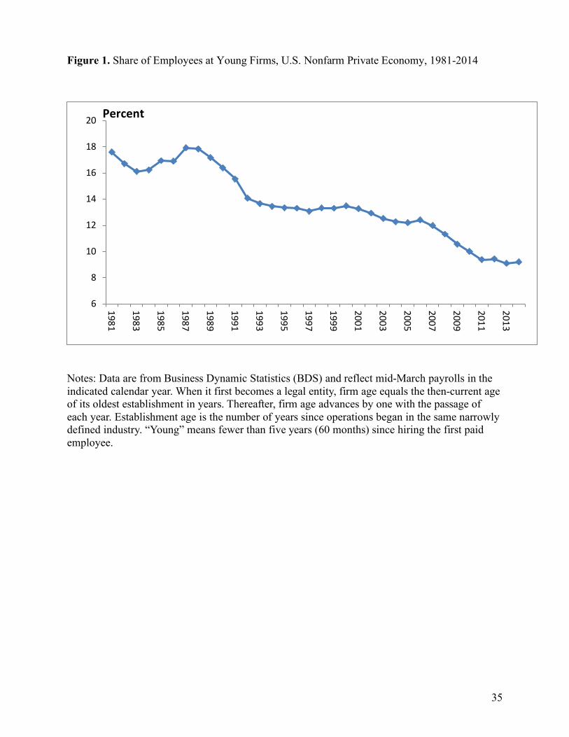
35

Figure 1. Share of Employees at Young Firms, U.S. Nonfarm Private Economy, 1981-2014

Notes: Data are from Business Dynamic Statistics (BDS) and reflect mid-March payrolls in the indicated calendar year. When it first becomes a legal entity, firm age equals the then-current age of its oldest establishment in years. Thereafter, firm age advances by one with the passage of each year. Establishment age is the number of years since operations began in the same narrowly defined industry. “Young” means fewer than five years (60 months) since hiring the first paid employee.

6

8

10

12

14

16

18

20

1981

1983

1985

1987

1989

1991

1993

1995

1997

1999

2001

2003

2005

2007

2009

2011

2013

Percent

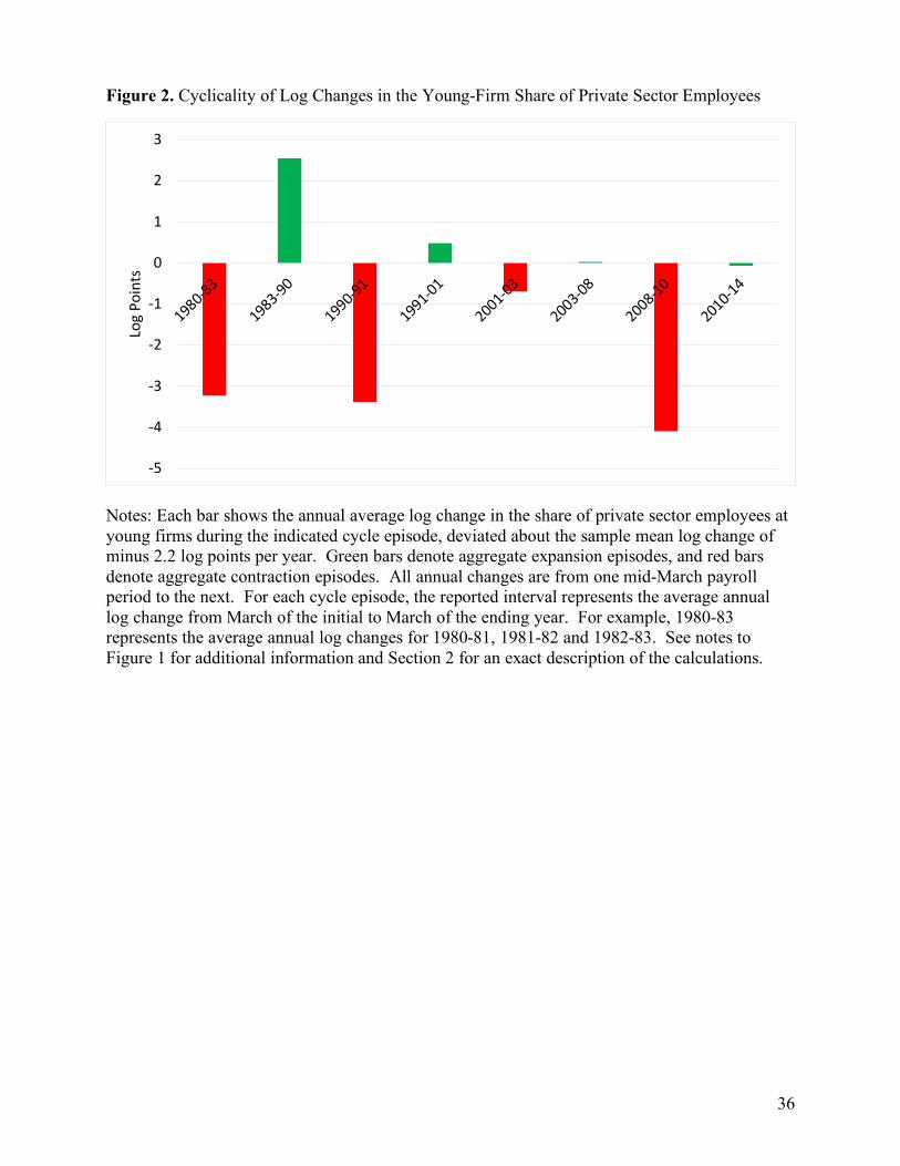
36

Figure 2. Cyclicality of Log Changes in the Young-Firm Share of Private Sector Employees

Notes: Each bar shows the annual average log change in the share of private sector employees at young firms during the indicated cycle episode, deviated about the sample mean log change of minus 2.2 log points per year. Green bars denote aggregate expansion episodes, and red bars denote aggregate contraction episodes. All annual changes are from one mid-March payroll period to the next. For each cycle episode, the reported interval represents the average annual log change from March of the initial to March of the ending year. For example, 1980-83 represents the average annual log changes for 1980-81, 1981-82 and 1982-83. See notes to Figure 1 for additional information and Section 2 for an exact description of the calculations.

-5

-4

-3

-2

-1

0

1

2

3

1980-83

1983-90

1990-91

1991-01

2001-03

2003-08

2008-10

2010-14

Log

Poin

ts

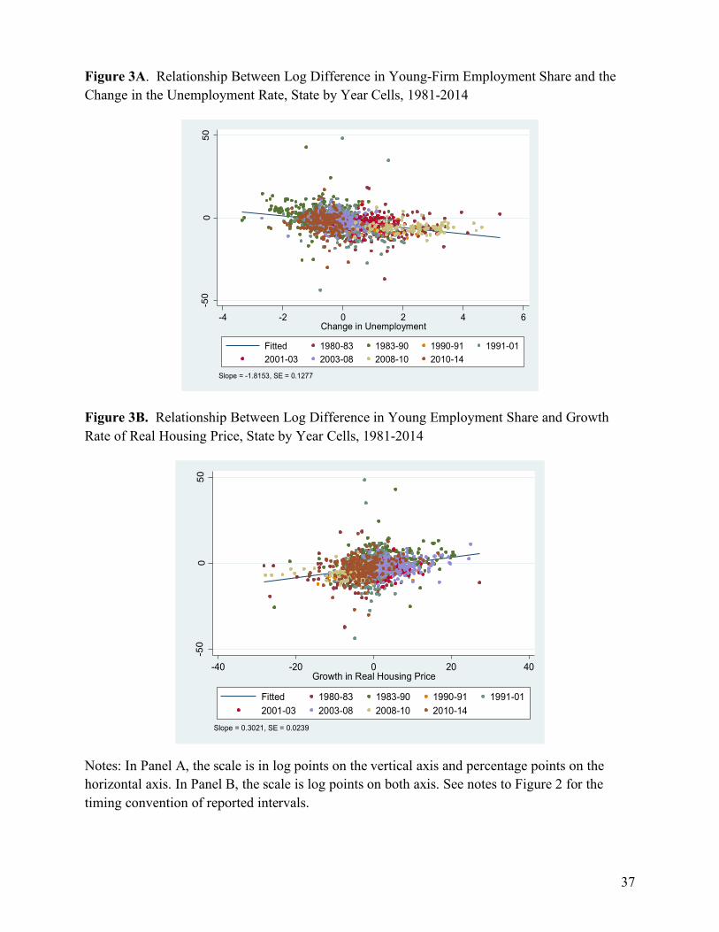
37

Figure 3A. Relationship Between Log Difference in Young-Firm Employment Share and the Change in the Unemployment Rate, State by Year Cells, 1981-2014

Figure 3B. Relationship Between Log Difference in Young Employment Share and Growth Rate of Real Housing Price, State by Year Cells, 1981-2014

Notes: In Panel A, the scale is in log points on the vertical axis and percentage points on the horizontal axis. In Panel B, the scale is log points on both axis. See notes to Figure 2 for the timing convention of reported intervals.

-50

050

Log

Diff

of Y

oung

Em

p S

hare

-4 -2 0 2 4 6Change in Unemployment

Fitted 1980-83 1983-90 1990-91 1991-012001-03 2003-08 2008-10 2010-14

Slope = -1.8153, SE = 0.1277

-50

05

0

Log

Diff of Y

oun

g E

mp S

ha

re

-40 -20 0 20 40

Growth in Real Housing Price

Fitted 1980-83 1983-90 1990-91 1991-01

2001-03 2003-08 2008-10 2010-14

Slope = 0.3021, SE = 0.0239

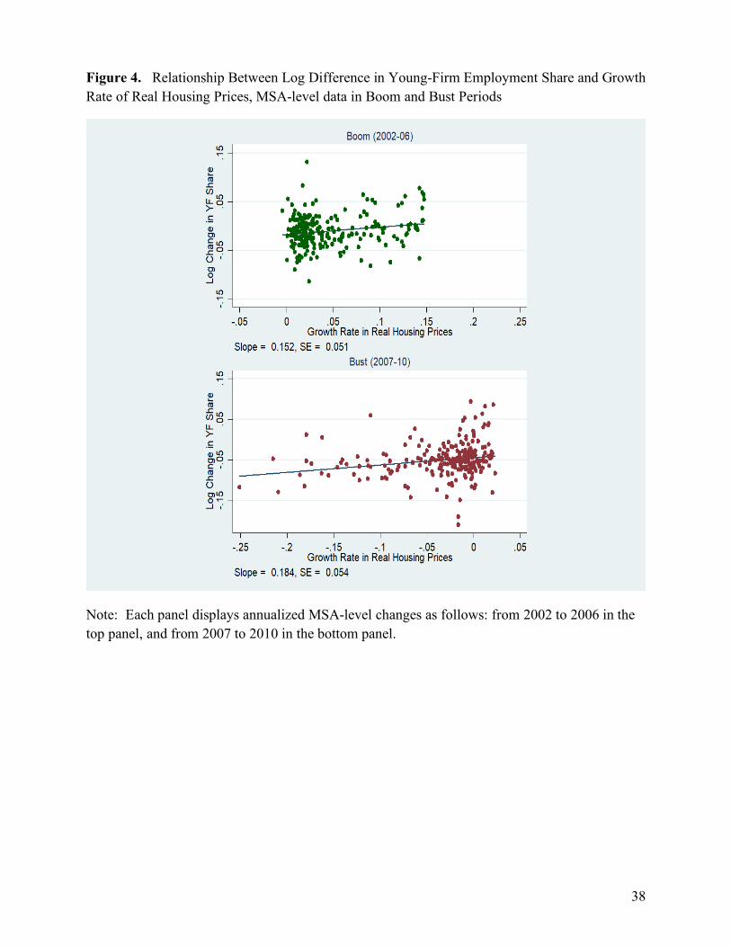
38

Figure 4. Relationship Between Log Difference in Young-Firm Employment Share and Growth Rate of Real Housing Prices, MSA-level data in Boom and Bust Periods

Note: Each panel displays annualized MSA-level changes as follows: from 2002 to 2006 in the top panel, and from 2007 to 2010 in the bottom panel.

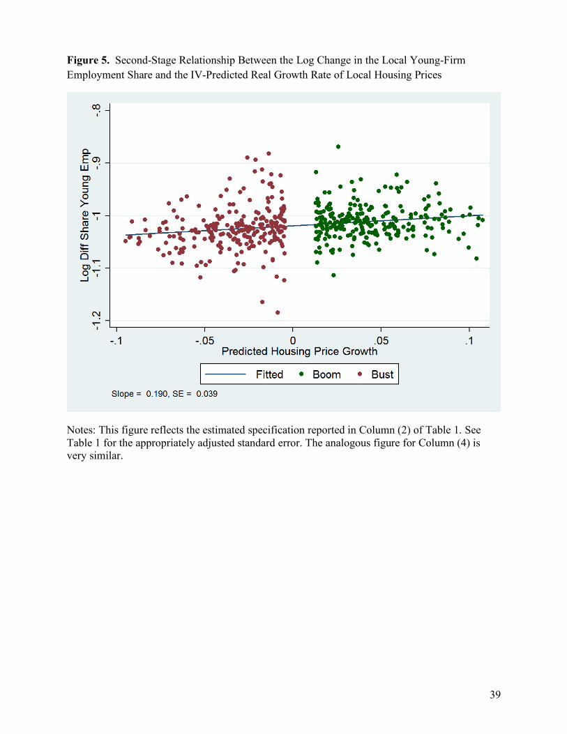
39

Figure 5. Second-Stage Relationship Between the Log Change in the Local Young-Firm Employment Share and the IV-Predicted Real Growth Rate of Local Housing Prices

Notes: This figure reflects the estimated specification reported in Column (2) of Table 1. See Table 1 for the appropriately adjusted standard error. The analogous figure for Column (4) is very similar.

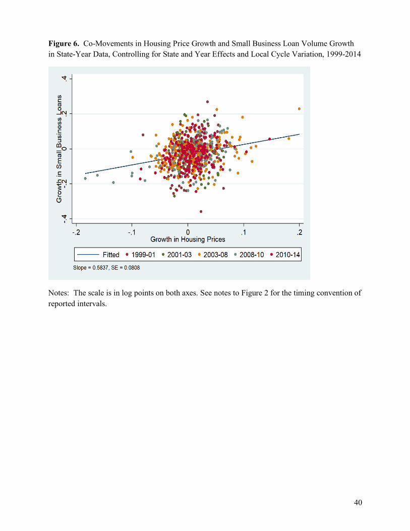
40

Figure 6. Co-Movements in Housing Price Growth and Small Business Loan Volume Growth in State-Year Data, Controlling for State and Year Effects and Local Cycle Variation, 1999-2014

Notes: The scale is in log points on both axes. See notes to Figure 2 for the timing convention of reported intervals.

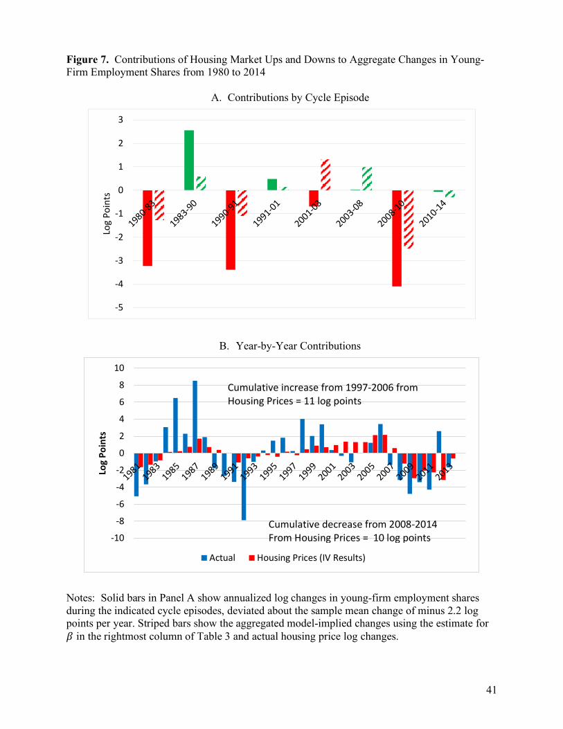
41

Figure 7. Contributions of Housing Market Ups and Downs to Aggregate Changes in Young-Firm Employment Shares from 1980 to 2014

A. Contributions by Cycle Episode

B. Year-by-Year Contributions

Notes: Solid bars in Panel A show annualized log changes in young-firm employment shares during the indicated cycle episodes, deviated about the sample mean change of minus 2.2 log points per year. Striped bars show the aggregated model-implied changes using the estimate for ? in the rightmost column of Table 3 and actual housing price log changes.

-5

-4

-3

-2

-1

0

1

2

3

1980-83

1983-90

1990-91

1991-01

2001-03

2003-08

2008-10

2010-14

Log

Poin

ts

-10

-8

-6

-4

-2

0

2

4

6

8

10

19811983

19851987

19891991

19931995

19971999

20012003

20052007

20092011

2013Log

Poin

ts

Actual Housing Prices (IV Results)

Cumulative increase from 1997-2006 fromHousing Prices = 11 log points

Cumulative decrease from 2008-2014 From Housing Prices = 10 log points

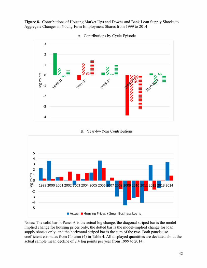
42

Figure 8. Contributions of Housing Market Ups and Downs and Bank Loan Supply Shocks to Aggregate Changes in Young-Firm Employment Shares from 1999 to 2014

A. Contributions by Cycle Episode

B. Year-by-Year Contributions

Notes: The solid bar in Panel A is the actual log change, the diagonal striped bar is the model-implied change for housing prices only, the dotted bar is the model-implied change for loan supply shocks only, and the horizontal striped bar is the sum of the two. Both panels use coefficient estimates from Column (4) in Table 4. All displayed quantities are deviated about the actual sample mean decline of 2.4 log points per year from 1999 to 2014.

-4

-3

-2

-1

0

1

2

3

1999-01

2001-03

2003-08

2008-10

2010-2014

Log

Poin

ts

-5-4-3-2-1012345

1999 2000 2001 2002 2003 2004 2005 2006 2007 2008 2009 2010 2011 2012 2013 2014Log

Poin

ts

Actual Housing Prices + Small Business Loans

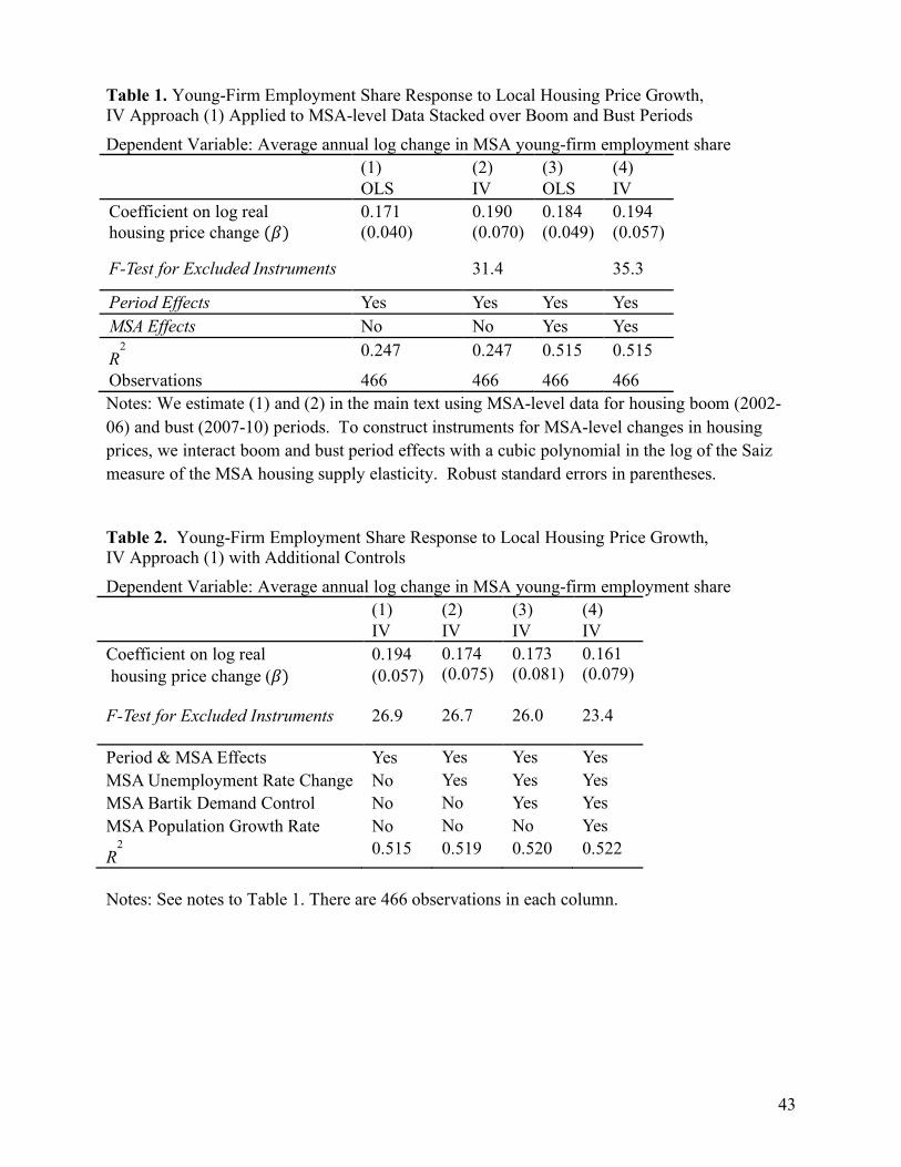
43

Table 1. Young-Firm Employment Share Response to Local Housing Price Growth, IV Approach (1) Applied to MSA-level Data Stacked over Boom and Bust Periods

Dependent Variable: Average annual log change in MSA young-firm employment share (1) (2) (3) (4) OLS IV OLS IV Coefficient on log real housing price change (?)

0.171 (0.040)

0.190 (0.070)

0.184 (0.049)

0.194 (0.057)

F-Test for Excluded Instruments 31.4 35.3

Period Effects Yes Yes Yes Yes MSA Effects No No Yes Yes

R2 0.247 0.247 0.515 0.515

Observations 466 466 466 466 Notes: We estimate (1) and (2) in the main text using MSA-level data for housing boom (2002-06) and bust (2007-10) periods. To construct instruments for MSA-level changes in housing prices, we interact boom and bust period effects with a cubic polynomial in the log of the Saiz measure of the MSA housing supply elasticity. Robust standard errors in parentheses. Table 2. Young-Firm Employment Share Response to Local Housing Price Growth, IV Approach (1) with Additional Controls

Dependent Variable: Average annual log change in MSA young-firm employment share (1) (2) (3) (4) IV IV IV IV Coefficient on log real housing price change (?)

0.194 (0.057)

0.174 (0.075)

0.173 (0.081)

0.161 (0.079)

F-Test for Excluded Instruments 26.9 26.7 26.0 23.4

Period & MSA Effects Yes Yes Yes Yes MSA Unemployment Rate Change No Yes Yes Yes MSA Bartik Demand Control No No Yes Yes MSA Population Growth Rate No No No Yes

R2 0.515 0.519 0.520 0.522

Notes: See notes to Table 1. There are 466 observations in each column.

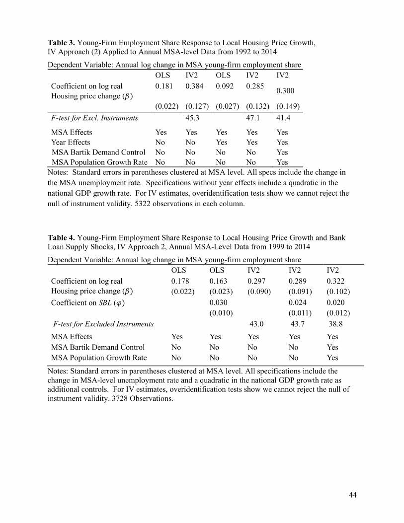
44

Table 3. Young-Firm Employment Share Response to Local Housing Price Growth, IV Approach (2) Applied to Annual MSA-level Data from 1992 to 2014

Dependent Variable: Annual log change in MSA young-firm employment share OLS IV2 OLS IV2 IV2 Coefficient on log real Housing price change (?)

0.181 0.384 0.092 0.285 0.300

(0.022) (0.127) (0.027) (0.132) (0.149) F-test for Excl. Instruments

45.3 47.1 41.4

MSA Effects Yes Yes Yes Yes Yes Year Effects No No Yes Yes Yes MSA Bartik Demand Control No No No No Yes MSA Population Growth Rate No No No No Yes

Notes: Standard errors in parentheses clustered at MSA level. All specs include the change in the MSA unemployment rate. Specifications without year effects include a quadratic in the national GDP growth rate. For IV estimates, overidentification tests show we cannot reject the null of instrument validity. 5322 observations in each column.

Table 4. Young-Firm Employment Share Response to Local Housing Price Growth and Bank Loan Supply Shocks, IV Approach 2, Annual MSA-Level Data from 1999 to 2014

Dependent Variable: Annual log change in MSA young-firm employment share OLS OLS IV2 IV2 IV2 Coefficient on log real Housing price change (?)

0.178 (0.022)

0.163 (0.023)

0.297 (0.090)

0.289 (0.091)

0.322 (0.102)

Coefficient on SBL (d) 0.030 (0.010)

0.024 (0.011)

0.020 (0.012)

F-test for Excluded Instruments 43.0 43.7 38.8 MSA Effects MSA Bartik Demand Control MSA Population Growth Rate

Yes No No

Yes No No

Yes No No

Yes No No

Yes Yes Yes

Notes: Standard errors in parentheses clustered at MSA level. All specifications include the change in MSA-level unemployment rate and a quadratic in the national GDP growth rate as additional controls. For IV estimates, overidentification tests show we cannot reject the null of instrument validity. 3728 Observations.

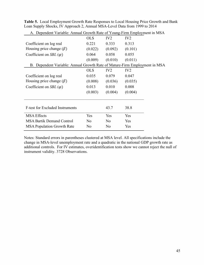
45

Table 5. Local Employment Growth Rate Responses to Local Housing Price Growth and Bank Loan Supply Shocks, IV Approach 2, Annual MSA-Level Data from 1999 to 2014

A. Dependent Variable: Annual Growth Rate of Young-Firm Employment in MSA OLS IV2 IV2 Coefficient on log real Housing price change (?)

0.221 (0.022)

0.333 (0.092)

0.313 (0.101)

Coefficient on SBL (d) 0.064 (0.009)

0.058 (0.010)

0.055 (0.011)

B. Dependent Variable: Annual Growth Rate of Mature-Firm Employment in MSA OLS IV2 IV2 Coefficient on log real Housing price change (?)

0.035 (0.008)

0.079 (0.036)

0.047 (0.035)

Coefficient on SBL (d) 0.013 (0.003)

0.010 (0.004)

0.008 (0.004)

F-test for Excluded Instruments

43.7

38.8

MSA Effects MSA Bartik Demand Control MSA Population Growth Rate

Yes No No

Yes No No

Yes Yes Yes

Notes: Standard errors in parentheses clustered at MSA level. All specifications include the change in MSA-level unemployment rate and a quadratic in the national GDP growth rate as additional controls. For IV estimates, overidentification tests show we cannot reject the null of instrument validity. 3728 Observations.

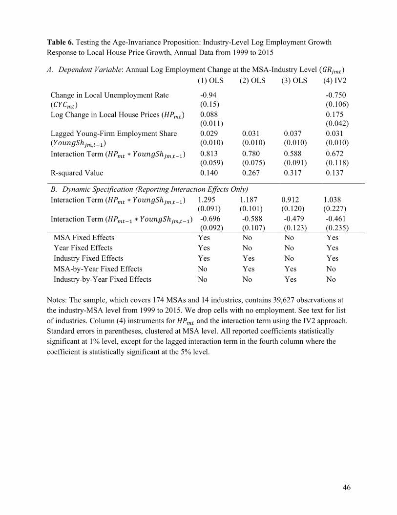
46

Table 6. Testing the Age-Invariance Proposition: Industry-Level Log Employment Growth Response to Local House Price Growth, Annual Data from 1999 to 2015

A. Dependent Variable: Annual Log Employment Change at the MSA-Industry Level (fgZ;") (1) OLS (2) OLS (3) OLS (4) IV2

Change in Local Unemployment Rate (W:W;")

-0.94 (0.15)

-0.750 (0.106)

Log Change in Local House Prices (@A;") 0.088 (0.011)

0.175 (0.042)

Lagged Young-Firm Employment Share (:kl8Y\ℎZ;,"'()

0.029 (0.010)

0.031 (0.010)

0.037 (0.010)

0.031 (0.010)

Interaction Term (@A;" ∗ :kl8Y\ℎZ;,"'() 0.813 (0.059)

0.780 (0.075)

0.588 (0.091)

0.672 (0.118)

R-squared Value 0.140 0.267 0.317 0.137

B. Dynamic Specification (Reporting Interaction Effects Only) Interaction Term (@A;" ∗ :kl8Y\ℎZ;,"'() 1.295

(0.091) 1.187 (0.101)

0.912 (0.120)

1.038 (0.227)

Interaction Term (@A;"'( ∗ :kl8Y\ℎZ;,"'() -0.696 (0.092)

-0.588 (0.107)

-0.479 (0.123)

-0.461 (0.235)

MSA Fixed Effects Yes No No Yes Year Fixed Effects Yes No No Yes Industry Fixed Effects Yes Yes No Yes MSA-by-Year Fixed Effects No Yes Yes No Industry-by-Year Fixed Effects No No Yes No

Notes: The sample, which covers 174 MSAs and 14 industries, contains 39,627 observations at the industry-MSA level from 1999 to 2015. We drop cells with no employment. See text for list of industries. Column (4) instruments for @A;" and the interaction term using the IV2 approach. Standard errors in parentheses, clustered at MSA level. All reported coefficients statistically significant at 1% level, except for the lagged interaction term in the fourth column where the coefficient is statistically significant at the 5% level.

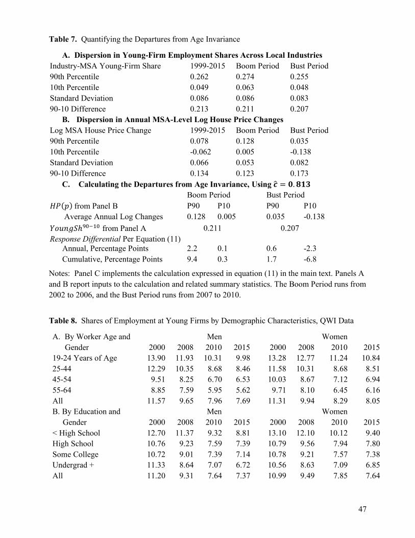
47

Table 7. Quantifying the Departures from Age Invariance

A. Dispersion in Young-Firm Employment Shares Across Local Industries Industry-MSA Young-Firm Share 1999-2015 Boom Period Bust Period 90th Percentile 0.262 0.274 0.255 10th Percentile 0.049 0.063 0.048 Standard Deviation 0.086 0.086 0.083 90-10 Difference 0.213 0.211 0.207

B. Dispersion in Annual MSA-Level Log House Price Changes Log MSA House Price Change 1999-2015 Boom Period Bust Period 90th Percentile 0.078 0.128 0.035 10th Percentile -0.062 0.005 -0.138 Standard Deviation 0.066 0.053 0.082 90-10 Difference 0.134 0.123 0.173

C. Calculating the Departures from Age Invariance, Using âä = ã. åçé Boom Period Bust Period @A(w)from Panel B P90 P10 P90 P10 Average Annual Log Changes 0.128 0.005 0.035 -0.138 :kl8Y\ℎ|+'(+ from Panel A 0.211 0.207 Response Differential Per Equation (11) Annual, Percentage Points 2.2 0.1 0.6 -2.3 Cumulative, Percentage Points 9.4 0.3 1.7 -6.8

Notes: Panel C implements the calculation expressed in equation (11) in the main text. Panels A and B report inputs to the calculation and related summary statistics. The Boom Period runs from 2002 to 2006, and the Bust Period runs from 2007 to 2010.

Table 8. Shares of Employment at Young Firms by Demographic Characteristics, QWI Data

A. By Worker Age and Men Women Gender 2000 2008 2010 2015 2000 2008 2010 2015 19-24 Years of Age 13.90 11.93 10.31 9.98 13.28 12.77 11.24 10.84 25-44 12.29 10.35 8.68 8.46 11.58 10.31 8.68 8.51 45-54 9.51 8.25 6.70 6.53 10.03 8.67 7.12 6.94 55-64 8.85 7.59 5.95 5.62 9.71 8.10 6.45 6.16 All 11.57 9.65 7.96 7.69 11.31 9.94 8.29 8.05 B. By Education and Men Women Gender 2000 2008 2010 2015 2000 2008 2010 2015 < High School 12.70 11.37 9.32 8.81 13.10 12.10 10.12 9.40 High School 10.76 9.23 7.59 7.39 10.79 9.56 7.94 7.80 Some College 10.72 9.01 7.39 7.14 10.78 9.21 7.57 7.38 Undergrad + 11.33 8.64 7.07 6.72 10.56 8.63 7.09 6.85 All 11.20 9.31 7.64 7.37 10.99 9.49 7.85 7.64

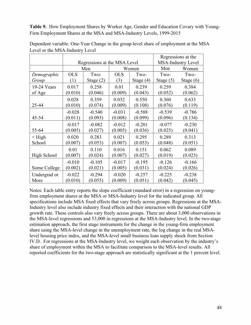
48

Table 9. How Employment Shares by Worker Age, Gender and Education Covary with Young-Firm Employment Shares at the MSA and MSA-Industry Levels, 1999-2015

Dependent variable: One-Year Change in the group-level share of employment at the MSA Level or the MSA-Industry Level

Regressions at the MSA Level Regressions at the

MSA-Industry Level Men Women Men Women Demographic Group

OLS (1)

Two-Stage (2)

OLS (3)

Two-Stage (4)

Two-Stage (5)

Two-Stage (6)

19-24 Years of Age

0.017 (0.010)

0.258 (0.046)

0.01 (0.009)

0.239 (0.043)

0.259 (0.052)

0.384 (0.062)

25-44 0.028

(0.010) 0.359

(0.074) 0.032

(0.009) 0.550

(0.108) 0.360

(0.076) 0.633

(0.119)

45-54 -0.028 (0.011)

-0.540 (0.093)

-0.031 (0.008)

-0.588 (0.099)

-0.539 (0.096)

-0.786 (0.134)

55-64 -0.017 (0.005)

-0.082 (0.027)

-0.012 (0.005)

-0.201 (0.036)

-0.077 (0.025)

-0.230 (0.041)

< High School

0.020 (0.007)

0.283 (0.053)

0.021 (0.007)

0.295 (0.053)

0.289 (0.048)

0.313 (0.051)

High School 0.01

(0.007) 0.110

(0.024) 0.016

(0.007) 0.151

(0.027) 0.062

(0.019) 0.089

(0.023)

Some College -0.010 (0.002)

-0.105 (0.021)

-0.017 (0.005)

-0.195 (0.031)

-0.126 (0.024)

-0.166 (0.026)

Undergrad or More

-0.022 (0.010)

-0.294 (0.055)

-0.020 (0.009)

-0.257 (0.051)

-0.225 (0.042)

-0.238 (0.045)

Notes: Each table entry reports the slope coefficient (standard error) in a regression on young-firm employment shares at the MSA or MSA-Industry level for the indicated group. All specifications include MSA fixed effects that vary freely across groups. Regressions at the MSA-Industry level also include industry fixed effects and their interaction with the national GDP growth rate. These controls also vary freely across groups. There are about 3,000 observations in the MSA-level regressions and 53,000 in regressions at the MSA-Industry level. In the two-stage estimation approach, the first stage instruments for the change in the young-firm employment share using the MSA-level change in the unemployment rate, the log change in the real MSA-level housing price index, and the MSA-level small business loan supply shock from Section IV.D. For regressions at the MSA-Industry level, we weight each observation by the industry’s share of employment within the MSA to facilitate comparison to the MSA-level results. All reported coefficients for the two-stage approach are statistically significant at the 1 percent level.

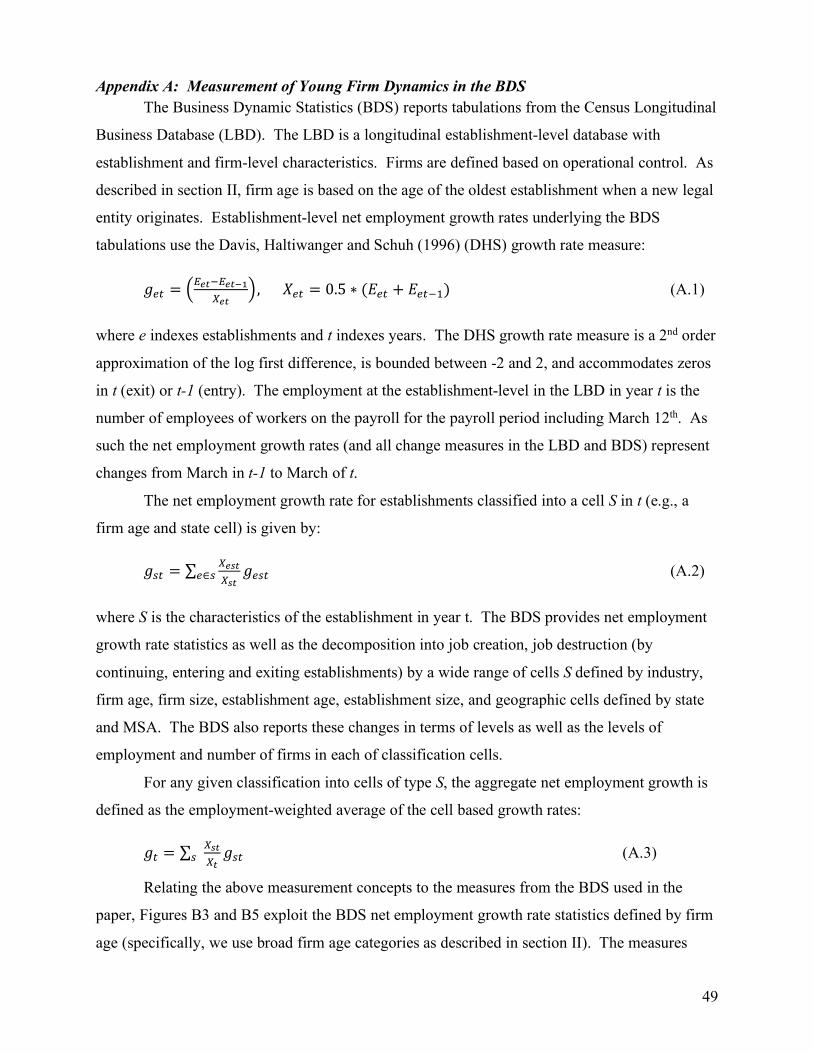
49

Appendix A: Measurement of Young Firm Dynamics in the BDS The Business Dynamic Statistics (BDS) reports tabulations from the Census Longitudinal

Business Database (LBD). The LBD is a longitudinal establishment-level database with

establishment and firm-level characteristics. Firms are defined based on operational control. As

described in section II, firm age is based on the age of the oldest establishment when a new legal

entity originates. Establishment-level net employment growth rates underlying the BDS

tabulations use the Davis, Haltiwanger and Schuh (1996) (DHS) growth rate measure:

Yè" = êëíì'ëíìîïñíì

ó,Oè" = 0.5 ∗ (!è" + !è"'() (A.1)

where e indexes establishments and t indexes years. The DHS growth rate measure is a 2nd order

approximation of the log first difference, is bounded between -2 and 2, and accommodates zeros

in t (exit) or t-1 (entry). The employment at the establishment-level in the LBD in year t is the

number of employees of workers on the payroll for the payroll period including March 12th. As

such the net employment growth rates (and all change measures in the LBD and BDS) represent

changes from March in t-1 to March of t.

The net employment growth rate for establishments classified into a cell S in t (e.g., a

firm age and state cell) is given by:

Y<" = ∑ ñíòìñòìè∈< Yè<" (A.2)

where S is the characteristics of the establishment in year t. The BDS provides net employment

growth rate statistics as well as the decomposition into job creation, job destruction (by

continuing, entering and exiting establishments) by a wide range of cells S defined by industry,

firm age, firm size, establishment age, establishment size, and geographic cells defined by state

and MSA. The BDS also reports these changes in terms of levels as well as the levels of

employment and number of firms in each of classification cells.

For any given classification into cells of type S, the aggregate net employment growth is

defined as the employment-weighted average of the cell based growth rates:

Y" = ∑ ñòìñì< Y<" (A.3)

Relating the above measurement concepts to the measures from the BDS used in the

paper, Figures B3 and B5 exploit the BDS net employment growth rate statistics defined by firm

age (specifically, we use broad firm age categories as described in section II). The measures

50

used in these figures capture within firm age group net employment growth rates. While

instructive, such within firm age group net growth rates don’t permit a characterization of the

changing composition of employment by firm age (and likewise the changing composition of

firms by firm age). For the latter, we use the share of young firm employment and the share of

young firms as described in the main text. These can be directly measured from the BDS since

the number of employees and firms are reported for all classifications in the BDS. Section III

includes discussion of how the changing employment by firm age is related to net change within

firm age groups and the changing composition.

Firm age is censored in the BDS given that firm and establishment age cannot be

determined for establishments that exist in 1976 (the first year of the LBD). This implies that in

each year subsequent to 1976 more firm age categories can be defined. We commence our

analysis in 1981 where five firm age categories can be defined: firm age 0 (establishments in

1981 whose parent firm have all new establishments in 1981), 1, 2, 3, 4 and 5+. This permits

consistent measures of young firm activity measures starting in 1981. For example, in 1981 we

can measure net employment growth rates for young firms which reflects the growth rate of the

establishments from March 1980 to March 1981.

The BDS also provides the statistics to compute directly the employment of young firms

(less than five years old) starting in 1981. We use the young-employment shares to compute the

log change in the share of young-firm employment which, our focus in the main text. This

measure is directly computable from BDS statistics starting in 1982 (e.g., the log change in 1982

is the log difference of the young-firm share from 1981 to 1982). Given the focus on cyclical

episodes in our analysis, it is advantageous to define the early 1980s cyclical downturn as the

March 1980 to March 1983 interval. This requires measures of the relevant change statistics

starting in 1981. For net employment growth rates young firms in Figures B3 and B5, this is

readily computable from the BDS. For the log change in the young-firm employment share in

1981, additional computations are required. In 1980, the BDS yields the employment of firms

less than four years old directly, but to measure the employment of firms less than five years old

in 1980 we need an estimate of employment at firms age=4 in 1980. We impute the latter in

1980 using the product of the share of employment of age=4 year firms in 1981 and total

employment in 1980. This imputation is feasible at the national, state and MSA levels of

aggregation. We note that all of our results using the log change in the young-firm employment

share are robust to starting the analysis in 1982 instead of 1981.

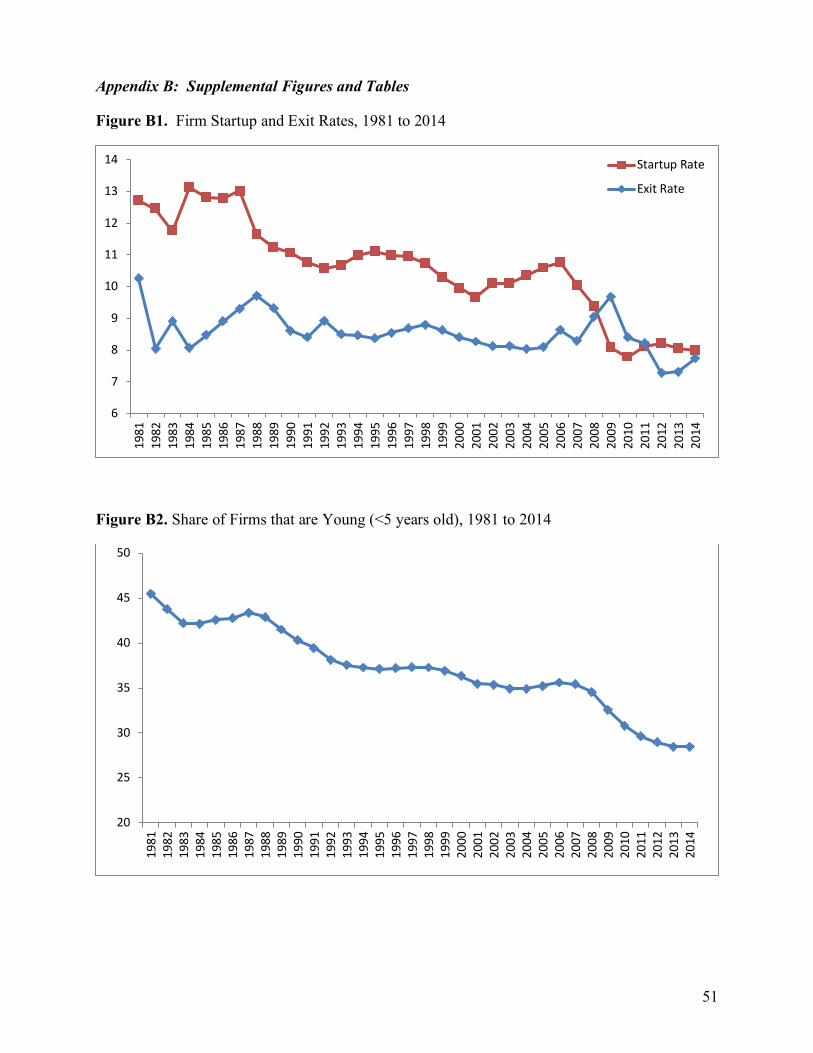
51

Appendix B: Supplemental Figures and Tables

Figure B1. Firm Startup and Exit Rates, 1981 to 2014

Figure B2. Share of Firms that are Young (<5 years old), 1981 to 2014

6

7

8

9

10

11

12

13

1419

8119

8219

8319

8419

8519

8619

8719

8819

8919

9019

9119

9219

9319

9419

9519

9619

9719

9819

9920

0020

0120

0220

0320

0420

0520

0620

0720

0820

0920

1020

1120

1220

1320

14

Startup Rate

Exit Rate

20

25

30

35

40

45

50

1981

1982

1983

1984

1985

1986

1987

1988

1989

1990

1991

1992

1993

1994

1995

1996

1997

1998

1999

2000

2001

2002

2003

2004

2005

2006

2007

2008

2009

2010

2011

2012

2013

2014

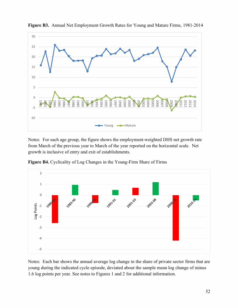
52

Figure B3. Annual Net Employment Growth Rates for Young and Mature Firms, 1981-2014

Notes: For each age group, the figure shows the employment-weighted DHS net growth rate from March of the previous year to March of the year reported on the horizontal scale. Net growth is inclusive of entry and exit of establishments.

Figure B4. Cyclicality of Log Changes in the Young-Firm Share of Firms

Notes: Each bar shows the annual average log change in the share of private sector firms that are young during the indicated cycle episode, deviated about the sample mean log change of minus 1.6 log points per year. See notes to Figures 1 and 2 for additional information.

-10

-5

0

5

10

15

20

25

30

1981198219831984198519861987198819891990199119921993199419951996199719981999200020012002200320042005200620072008200920102011201220132014

Young Mature

-5

-4

-3

-2

-1

0

1

2

1980-83

1983-90

1990-91

1991-01

2001-03

2003-08

2008-10

2010-14

Log

Poin

ts

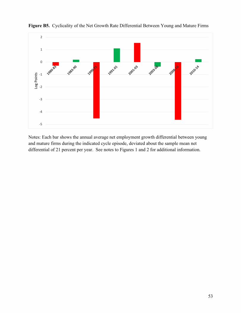
53

Figure B5. Cyclicality of the Net Growth Rate Differential Between Young and Mature Firms

Notes: Each bar shows the annual average net employment growth differential between young and mature firms during the indicated cycle episode, deviated about the sample mean net differential of 21 percent per year. See notes to Figures 1 and 2 for additional information.

-5

-4

-3

-2

-1

0

1

2

1980-83

1983-90

1990-91

1991-01

2001-03

2003-08

2008-10

2010-14

Log

Poin

ts

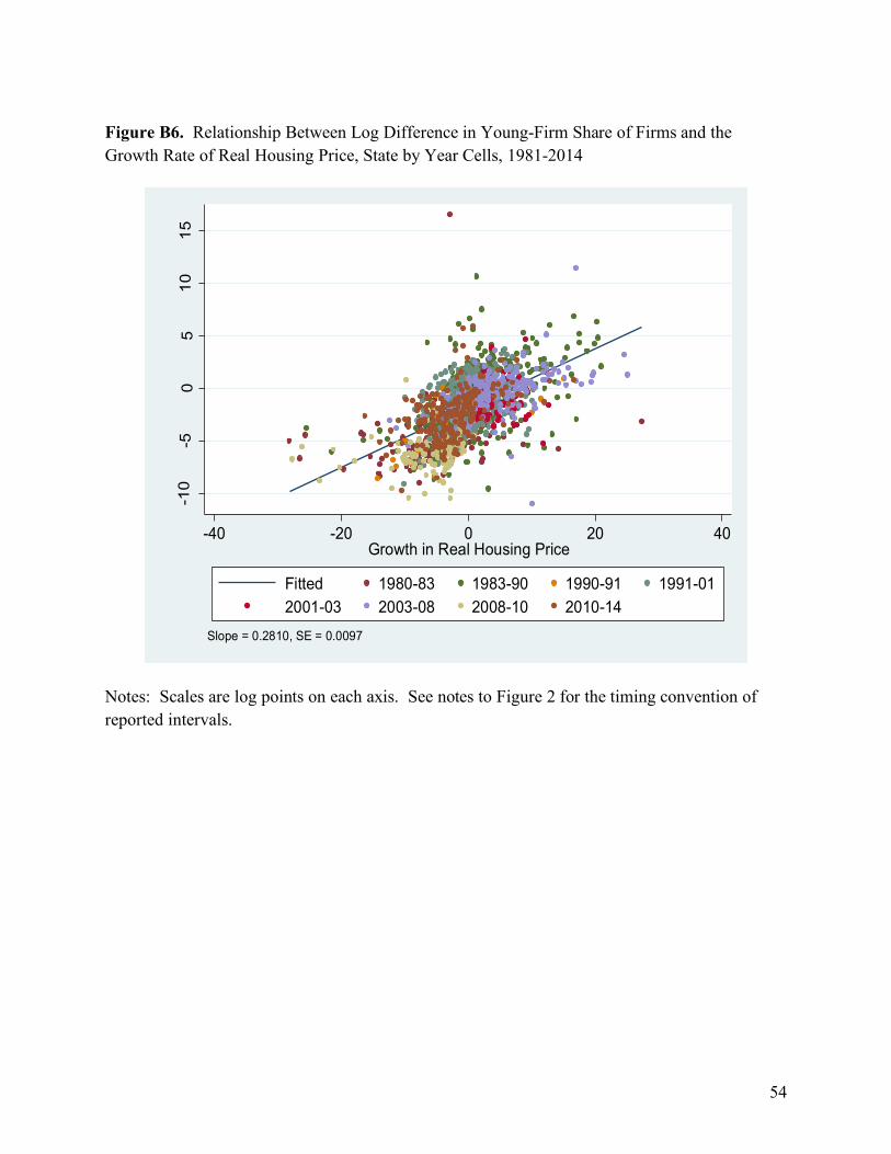
54

Figure B6. Relationship Between Log Difference in Young-Firm Share of Firms and the Growth Rate of Real Housing Price, State by Year Cells, 1981-2014

Notes: Scales are log points on each axis. See notes to Figure 2 for the timing convention of reported intervals.

-10

-50

51

01

5

Log

Diff of Y

oun

g F

irm

Sh

are

-40 -20 0 20 40

Growth in Real Housing Price

Fitted 1980-83 1983-90 1990-91 1991-01

2001-03 2003-08 2008-10 2010-14

Slope = 0.2810, SE = 0.0097

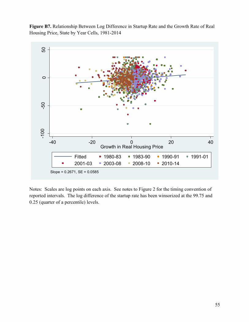
55

Figure B7. Relationship Between Log Difference in Startup Rate and the Growth Rate of Real Housing Price, State by Year Cells, 1981-2014

Notes: Scales are log points on each axis. See notes to Figure 2 for the timing convention of reported intervals. The log difference of the startup rate has been winsorized at the 99.75 and 0.25 (quarter of a percentile) levels.

-100

-50

050

Log

Diff

of s

tartu

p E

mp

Sha

re

-40 -20 0 20 40Growth in Real Housing Price

Fitted 1980-83 1983-90 1990-91 1991-012001-03 2003-08 2008-10 2010-14

Slope = 0.2671, SE = 0.0585

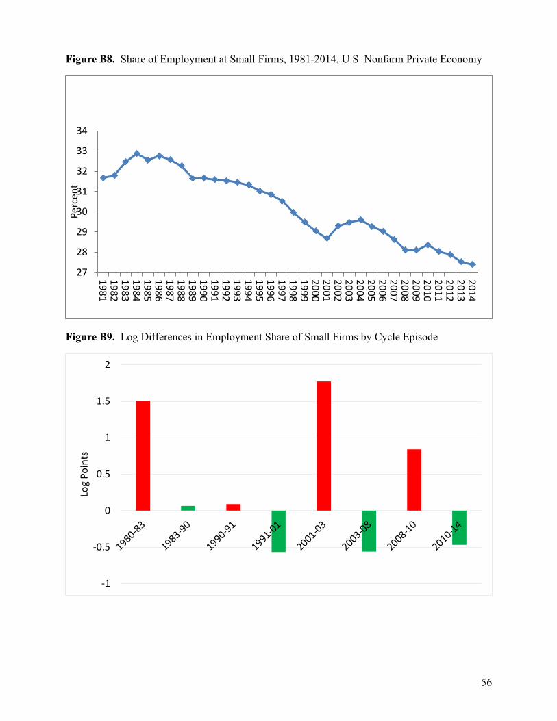
56

Figure B8. Share of Employment at Small Firms, 1981-2014, U.S. Nonfarm Private Economy

Figure B9. Log Differences in Employment Share of Small Firms by Cycle Episode

27

28

29

30

31

32

33

34

1981198219831984198519861987198819891990199119921993199419951996199719981999200020012002200320042005200620072008200920102011201220132014

Perc

ent

-1

-0.5

0

0.5

1

1.5

2

1980-83

1983-90

1990-91

1991-01

2001-03

2003-08

2008-10

2010-14

Log

Poin

ts

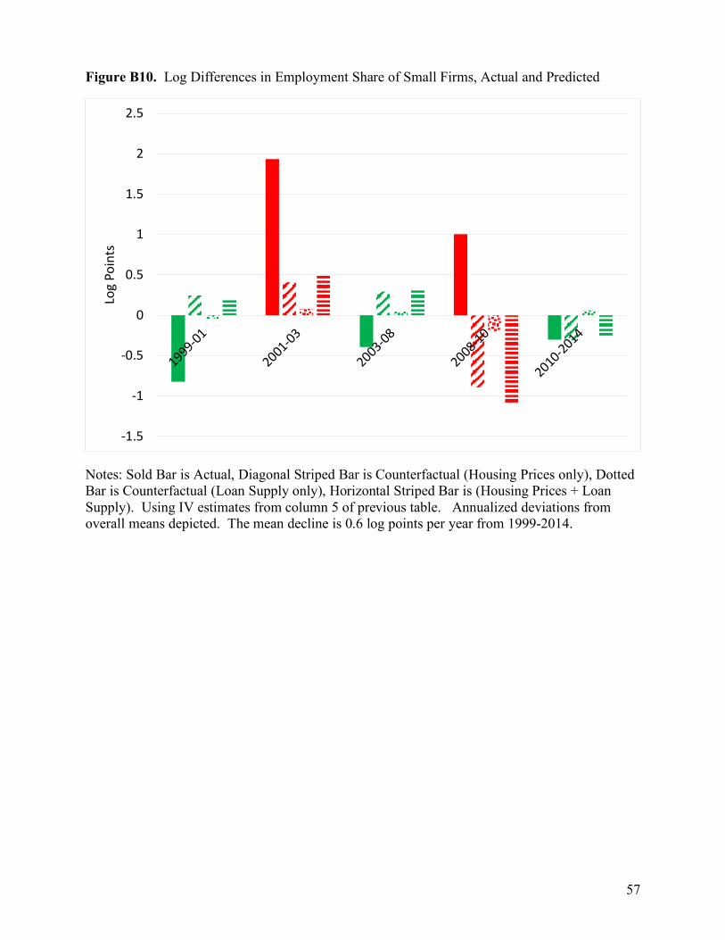
57

Figure B10. Log Differences in Employment Share of Small Firms, Actual and Predicted

Notes: Sold Bar is Actual, Diagonal Striped Bar is Counterfactual (Housing Prices only), Dotted Bar is Counterfactual (Loan Supply only), Horizontal Striped Bar is (Housing Prices + Loan Supply). Using IV estimates from column 5 of previous table. Annualized deviations from overall means depicted. The mean decline is 0.6 log points per year from 1999-2014.

-1.5

-1

-0.5

0

0.5

1

1.5

2

2.5

1999-01

2001-03

2003-08

2008-10

2010-2014

Log

Poin

ts

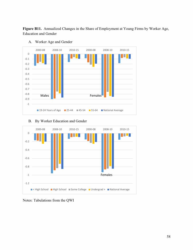
58

Figure B11. Annualized Changes in the Share of Employment at Young Firms by Worker Age, Education and Gender

A. Worker Age and Gender

B. By Worker Education and Gender

Notes: Tabulations from the QWI

-1

-0.9

-0.8

-0.7

-0.6

-0.5

-0.4

-0.3

-0.2

-0.1

02000-08 2008-10 2010-15 2000-08 2008-10 2010-15

19-24 Years of Age 25-44 45-54 55-64 National Average

Males Females

-1.2

-1

-0.8

-0.6

-0.4

-0.2

02000-08 2008-10 2010-15 2000-08 2008-10 2010-15

< High School High School Some College Undergrad + National Average

Females

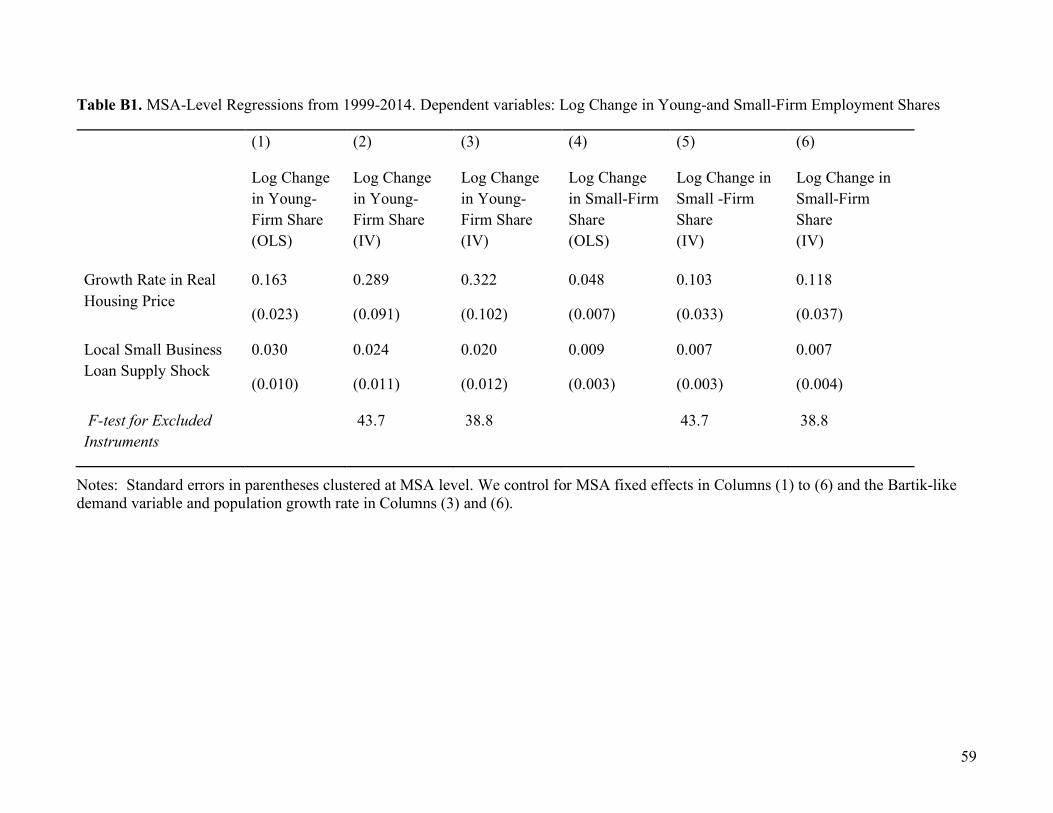
59

Table B1. MSA-Level Regressions from 1999-2014. Dependent variables: Log Change in Young-and Small-Firm Employment Shares

(1) (2) (3) (4) (5) (6)

Log Change in Young-Firm Share (OLS)

Log Change in Young-Firm Share (IV)

Log Change in Young-Firm Share (IV)

Log Change in Small-Firm Share (OLS)

Log Change in Small -Firm Share (IV)

Log Change in Small-Firm Share (IV)

Growth Rate in Real Housing Price

0.163

(0.023)

0.289

(0.091)

0.322

(0.102)

0.048

(0.007)

0.103

(0.033)

0.118

(0.037)

Local Small Business Loan Supply Shock

0.030

(0.010)

0.024

(0.011)

0.020

(0.012)

0.009

(0.003)

0.007

(0.003)

0.007

(0.004)

F-test for Excluded Instruments

43.7 38.8 43.7 38.8

Notes: Standard errors in parentheses clustered at MSA level. We control for MSA fixed effects in Columns (1) to (6) and the Bartik-like demand variable and population growth rate in Columns (3) and (6).

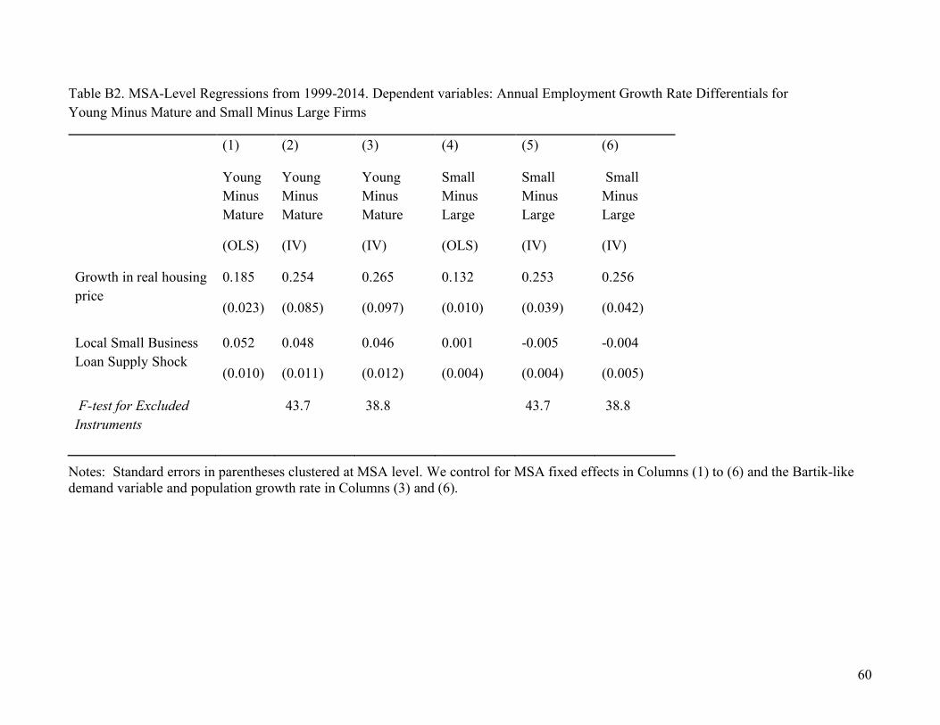
60

Table B2. MSA-Level Regressions from 1999-2014. Dependent variables: Annual Employment Growth Rate Differentials for Young Minus Mature and Small Minus Large Firms

(1) (2) (3) (4) (5) (6)

Young Minus Mature

(OLS)

Young Minus Mature

(IV)

Young Minus Mature

(IV)

Small Minus Large

(OLS)

Small Minus Large

(IV)

Small Minus Large

(IV)

Growth in real housing price

0.185

(0.023)

0.254

(0.085)

0.265

(0.097)

0.132

(0.010)

0.253

(0.039)

0.256

(0.042)

Local Small Business Loan Supply Shock

0.052

(0.010)

0.048

(0.011)

0.046

(0.012)

0.001

(0.004)

-0.005

(0.004)

-0.004

(0.005)

F-test for Excluded Instruments

43.7 38.8 43.7 38.8

Notes: Standard errors in parentheses clustered at MSA level. We control for MSA fixed effects in Columns (1) to (6) and the Bartik-like demand variable and population growth rate in Columns (3) and (6).

61

Appendix C: Details Related to the CRA Data and How We Use Them

CRA data provide bank-level information by local area and year on the volume of

business loan originations to firms with less than $1 million in revenue. We deflate nominal loan

volumes by the same-year GDP implicit price deflator from the Bureau of Economic Analysis to

obtain real small business loan volumes. As in GMN (2015), we roll up the bank level data to the

bank holding company, using data sources from the FDIC and Federal Reserve call reports. We

also use data from the Federal Reserve Bank of Chicago that tracks mergers and acquisitions, so

that for any pair of years t-1 and t we assign a bank to its owner in year t.

We measure the growth rate of small business loan volume for a given bank holding

company in a particular MSA – what we call !"#$in equation (6) – using the symmetric growth

rate measure in Davis, Haltiwanger and Schuh (1996). The DHS measure is equivalent to the log

first difference up to a second-order Taylor Series approximation, but the DHS measure down

weights outliers relative to log changes. As it turns out, DHS growth rates and log changes

produce similar econometric results in Section IV.d.

One additional detail: We re-time the calendar-year &'()$ measure in equation (7) to

align it with the March-to-March employment changes in the BDS. Specifically, in our

regression analysis, the loan supply shock for MSA m and year t is 0.75 ∗ Raw&'()$23 +

0.25 ∗ Raw&'()$. The correlation between this re-timed measure for year t and the unadjusted

measure for year t-1 is 0.95 for the MSA-level data used to produce Table 4. Replacing the re-

timed SBL measure for year t with the corresponding lagged Raw SBL measure yields very

similar results.