1

Dynamics of Unemployment and Home Price Shocks on Mortgage

Default Rates

Abstract This paper uses a Structural Vector Autoregression (SVAR) model to study the dynamics of the

impact of unemployment and home price index shocks on mortgage default rates from 1979 to

2000 and from 2001 to 2010. We first fit the model to the 1979 to 2000 sample and forecast the

changes in the national and regional mortgage default rates from 2001 to 2010. The model did a

good job in forecasting the actual changes in the mortgage default rates from 2001 to 2007;

however, it failed during 2008 to 2010. The results for the 1979 to 2000 and 2001 to 2010

periods indicate that the dynamic response of the mortgage default rate to unemployment and

home price index shocks changed at the national, regional and state levels after 2000.

Unemployment and home price shocks seem to have become more important during the 2001 to

2010 period. The two shocks are responsible on average for about 60% of the movement in the

regional mortgage default rates during this period. Except for the Pacific region, California and

Florida, most of the variations in the mortgage default rates at the national, regional and state

levels are explained by the unemployment shocks. The post 2000 results could be attributed to

the increase in the number of mortgage loan borrowers who were more susceptible to

unemployment and negative home price shocks.

Yaw Owusu-Ansah1

Economics Department, Columbia University

International Affairs Building, MC 3308

420 West 118th Street, New York NY 10027

yao2103@columbia.edu

Latest Edition: November 12th

, 2012

JEL Classification: C13, G21, R38

Key Words: Mortgage Default, Unemployment, Home Price Indices, SVAR

1 I wish to thank Brendan O’Flaherty and Bernard Salanie for their invaluable advice. I also thank Pierre-Andre

Chiappori, Rajiv Sethi, and Christopher Mayer.

2

1. Introduction

The traditional model of mortgage default posits that borrowers default if and only if they

have negative equity. A classic example is the option-based mortgage default model examined

by Foster and Van Order (1984) in which default is a put option. Borrowers would exercise the

put option when the value of the house plus any costs of exercising the option falls below the

mortgage value. However, recent studies2 have shown that many borrowers with negative equity

do not necessarily default. These borrowers continue to honor their contractual obligation to the

lenders even though their houses are worth less than the loans outstanding. These studies found

that default is often associated with a negative income shock; i.e. being unemployed usually is a

bigger factor than negative equity. Foote et al. (2009) found that a 1% increase in the

unemployment rate raises the probability of default by 10-20%, while a 10% point fall in housing

prices raises the probability of default by more than 50%. On the other hand, there have also

been documented cases where borrowers have exercised the option to default when they have

negative equity even though they could afford to pay their mortgages. Ashworth et al. (2010)

concluded that negative equity shocks are far more important predictor of mortgage defaults than

unemployment shocks. However, they also found that employment shocks can amplify the

default rate if the borrower has already experienced a negative equity shock. As Mayer et al

(2009) showed areas that experienced increased unemployment rates also experienced decline in

house prices. As such, it is not easy to establish whether defaults in these areas are due to

unemployment or house prices.

In this paper, we attempt to disentangle the interrelations between the home price index

(which tracks housing prices) and unemployment shocks and mortgage default rates by studying

the dynamics of these two shocks on mortgage default rates from 1979 to 2010. The 2001 to

2010 period represents a time when there have been significant changes in unemployment, house

price indices and mortgage default rate at the same time. As such, this period presents a perfect

period to empirically test which of these two shocks have had a bigger impact on mortgage

default rates. We also want to know how the dynamics of the impacts of these two shocks in

2001 to 2010 have deviated from their historical dynamics (1979 to 2000). Not only have there

been significant changes in these three variables during the 2001 to 2010 period, underwriting

standards also deteriorated significantly during the period as the growing number of subprime

2 Neil Bhutta et al. (2010)

3

loans originated during this period shows. Incentives in the mortgage market also shifted to the

“originate-to-distribute” model, under which mortgage brokers originated loans and then sold

them to institutions that securitized them. Because these brokers do not have to bear the cost of

default, they may not be stringent in screening potential mortgage borrowers (Keys, Mukherjee,

Seru, and Vig, 2008). About 700,000 subprime mortgage loans3 were originated annually

between 1998 and 2000 (Mayer and Pence, 2009); this increased to an average of 1.5 million

between 2003 and 2006 annual. Lax underwriting standards were not the only factor in the

increase in origination of subprime loans. A contributing factor was the house price appreciation

after 2001 which made subprime origination easier as homeowners could easily resell their

homes. Mayer and Pence (2009) documented that areas with high house price appreciation also

experienced an increase in subprime mortgage origination.

Given the different composition of mortgage borrowers and the different types of

mortgage loans originated during the two periods, a study of the impact of the unemployment

and home price shocks on mortgage defaults over these two periods is necessary.

Mortgage default rates are influenced by the unemployment and home price shocks at the

national, regional and state levels. However, describing the joint behavior of these three variables

is not easy. This paper utilizes a Structural Vector Autoregression (SVAR) to decompose the

national, regional and state mortgage default rates into unemployment and home price index

shocks. The data consist of unemployment rates, home price indices and mortgage default rates

at the national, regional4, and state

5 levels covering a period from 1979 to 2010 at a quarterly

frequency. The mortgage default rate is defined as the number of seriously delinquent mortgage

loans as a percentage of all loans serviced in each quarter. The seriously delinquent loans are

mortgage loans that are 90+ delinquent, i.e., they are loans for which the borrowers have not paid

the mortgage in 90+ days.

We first fit the SVAR model to the 1979 to 2000 national and regional data and forecast

the changes in the national and regional mortgage default rates for the 2001 to 2010 period. Not

only are we interested in how well the model performs out-of-sample, we are more interested in

its performance during the housing boom years of 2003 to 2006, and also during the recent Great

3 Subprime loans are usually targeted to borrowers who have bad credit, little savings available for a downpayment

and in some case no verifiable income or assets. 4 See Appendix A for more details about the census regions.

5 The states considered are Arizona, California, Florida, Michigan, Nevada and Pennsylvania.

4

Recession from 2008 to 2010. We examine the forecast errors from 2001 to 2010 and explore

some of the factors that might have contributed to the model not fitting the data well during the

Great Recession. We test for a structural break in the mortgage defaults rates during 2008 to

2010.

We then also estimate the model for the 2001 to 2010 sample and estimate the implied

impulse response functions from the identification for both the 1979 to 2000 and 2001 to 2010

periods for the national, regional and state data. This allows us to examine whether there have

been changes in the dynamics of the home price index and unemployment shocks on mortgage

default for both periods. Finally, we measure the importance of the two shocks in explaining the

changes in the mortgage default rate by performing variance decomposition for both sample

periods.

The forecasted changes in the national and regional mortgage default rates from 2001 to

2010 using estimated results from fitting the SVAR model to the 1979 to 2000 sample were not

far off from the actual changes in the mortgage default rates from 2001 to 2007. The model did

well even during the housing boom years of 2003 to 2006. However, the model failed to forecast

the changes in the mortgage default rates during the Great Recession. There has been a structural

break in the national and regional mortgage default rates during the 2008 to 2010 period which

could not have been anticipated by the model.

The empirical results also show that unemployment and home price index shocks on

average had very little impact on mortgage default rate at the national, regional and state level

during the 1979 to 2000 period. At the national level, an increase of one standard deviation in the

unemployment and home price index led to an increase of 1.3% and a decrease of 1% in the

mortgage default rate respectively during this period. At the regional level, the unemployment

and the home price index shocks produced on average an increase of 1.2% and a decrease of

1.1% respectively during the period. In comparison to 2001 to 2010 period, a standard deviation

increase in the national unemployment and the home price index shocks during this period led to

an increase of 7.2% and a decrease of 4.9% respectively in the national mortgage default rate. At

the regional level, there was an average increase of 12.9% for the unemployment shock and an

average decrease of 7.3% for the home price index shock during this period. On average, the

unemployment shocks seem to have had a bigger impact on the mortgage default rate than the

home price index shocks.

5

Also during the 2001 to 2010 period, the unemployment shocks explained on average

about 43% of the variation in the regional mortgage default rate, while the home price index

shocks explained on average about 20% of the variation in the regional mortgage default rate. In

effect, these two shocks were responsible on average for about 60% of the movement in the

regional mortgage default rates during this period. The two shocks explained very little of the

variation in the mortgage default rate during the 1979 to 2001 period.

The results indicate that the dynamic response of the mortgage default rate to

unemployment and home price index shocks changed at the national, regional and state levels

after 2000. Although there have been periods of higher national, regional and state

unemployment during the 1979 to 2000 period, they seemed to not have impacted the mortgage

default rates that much during this period. Except for the Pacific region, California and Florida,

unemployment shocks have had a bigger impact on the national, regional and state mortgage

default rates and can also explain more of the variation in the mortgage default rates than the

home price index shocks during the 2001 to 2010 period. The post 2000 results could be

attributed to the increase in the number of mortgage loan borrowers who were more susceptible

to unemployment and negative home price shocks. These borrowers have little savings they

could use to cushion them against unemployment and negative home price shocks. In their

papers, Mayer et al (2009), Demyanyk and Van Hemert (2008) and Mian and Sufi (2009) also

documented declining underwriting standards as a factor in mortgage default crises.

The paper proceeds as follows; Section 2 describes the SVAR model. Section 3 describes

the data used. Section 4 provides the results for the forecast errors from 2001 to 2010 and the

structural break tests. Section 5 provides the results for the impulse response functions and the

variance decompositions for the 1979 to 2000 and 2001 to 2010 periods. Section 6 provides

results for the impulse response functions and variance decompositions of the selected states.

Section 7 concludes.

6

2. SVAR Model

The goal of the empirical analysis is to assess the impact of unemployment and home price index

shocks on mortgage default rates. The SVAR system can be represented as:

( ) [

] [

] [

] [

]

where denotes the first difference of mortgage default rate, denotes the first difference of

unemployment rate and denotes the first difference of the home price index. Each is a

matrix.

Let [

] and [

] . Equation (1) can then be written as

( )

The innovations ( ) and [ ] for all . Multiplying equation (2) by

matrix , equation (2) can then be represented as:

( ) [

]

Where is the lag operator, are matrices of parameters, and is a

vector of orthogonalized disturbances: i.e. ( ) and [ ] for all .

It is usually better to transform into mutually uncorrelated innovations before we can

effectively analyze the effect of one time increase in the element of on the element

of . Let be a matrix such that: . Then

6 { (

) }

and { } . These transformations of the innovations allow us to analyze the

dynamics of the system in terms of a change to an element of . 6 { (

) } {

} ( )

( )

7

2.1 Short-Run Identification

In a short-run SVAR model, identification is obtained by placing restrictions on

matrices which are assumed to be nonsingular. At least 3 identifying restrictions are needed to be

imposed to achieve unique identification. We impose restrictions on the SVAR system by

applying equality constraints with the constraint matrices:

[

] and [

]

Because ( ) , the identification scheme implies that changes in the

unemployment rates are not contemporaneously affected by the changes in the home price

indices and the mortgage default rates. It also implies that changes in the mortgage default rates

are affected by the contemporaneous changes in the unemployment rates (if ) but not the

house price indices. Finally, it also implies that changes in the home price indices (if )

are affected by contemporaneous changes in the unemployment rates and the mortgage default

rates (if ).

Contemporaneous Effects

We have enough restrictions that the innovations and the associated unique impulse

responses are just-identified. We believe this identification strategy is reasonable: unemployed

borrowers will experience difficulties paying their mortgages thereby leading to an increase in

Unemployment

Default Rate Home Price

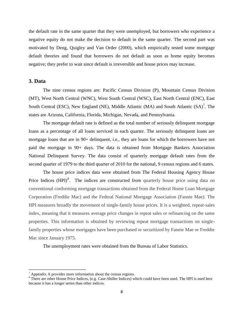
8

the default rate in the same quarter that they were unemployed, but borrowers who experience a

negative equity do not make the decision to default in the same quarter. The second part was

motivated by Deng, Quigley and Van Order (2000), which empirically tested some mortgage

default theories and found that borrowers do not default as soon as home equity becomes

negative; they prefer to wait since default is irreversible and house prices may increase.

3. Data

The nine census regions are: Pacific Census Division (P), Mountain Census Division

(MT), West North Central (WNC), West South Central (WSC), East North Central (ENC), East

South Central (ESC), New England (NE), Middle Atlantic (MA) and South Atlantic (SA)7. The

states are Arizona, California, Florida, Michigan, Nevada, and Pennsylvania.

The mortgage default rate is defined as the total number of seriously delinquent mortgage

loans as a percentage of all loans serviced in each quarter. The seriously delinquent loans are

mortgage loans that are in 90+ delinquent, i.e., they are loans for which the borrowers have not

paid the mortgage in 90+ days. The data is obtained from Mortgage Bankers Association

National Delinquent Survey. The data consist of quarterly mortgage default rates from the

second quarter of 1979 to the third quarter of 2010 for the national, 9 census regions and 6 states.

The house price indices data were obtained from The Federal Housing Agency House

Price Indices (HPI)8. The indices are constructed from quarterly house price using data on

conventional conforming mortgage transactions obtained from the Federal Home Loan Mortgage

Corporation (Freddie Mac) and the Federal National Mortgage Association (Fannie Mae). The

HPI measures broadly the movement of single-family house prices. It is a weighted, repeat-sales

index, meaning that it measures average price changes in repeat sales or refinancing on the same

properties. This information is obtained by reviewing repeat mortgage transactions on single-

family properties whose mortgages have been purchased or securitized by Fannie Mae or Freddie

Mac since January 1975.

The unemployment rates were obtained from the Bureau of Labor Statistics.

7 Appendix A provides more information about the census regions.

8 There are other House Price Indices, (e.g. Case-Shiller Indices) which could have been used. The HPI is used here

because it has a longer series than other indices.

9

4. Empirical Results

This section discusses the results of the forecast errors from 2001 to 2010 for the regional

and national mortgage default rates using the SVAR estimates from 1979 to 2000.

4.1 Forecast Errors of Mortgage Default Rate: 2001 to 2010 Period

Given the SVAR system:

( ) [

]

The optimal forecast (after ) of the system is given by:

( )9 ( ) ( ) ( )

The forecast error for the mortgage default rate is represented as:

( )

( )

Where is the national and regional mortgage default rate observed at time

and ( ) is the forecasted national and regional mortgage default rate at time .

Figures10

1 to 4 represent the graphs of the forecast errors for the national and New

England, East South Central and Mountain regions. The SVAR model was not far off in

forecasting the changes in the national and regional mortgage default rates from 2001 to 2007.

The big deviations in the forecast errors from 2006 to 2007 for the national and East South

Central—which are also present in the forecast error graph for West South Central—are due to

the effects of Hurricane Katrina. The model did a good job in forecasting the changes in the

mortgage default rate even in the housing boom years from 2003 to 2006. However, the model

failed during the Great Recession period (2008 to 2010). Section 4.2 explores some of the

reasons behind this forecast failure.

9 More information on the estimation of the forecast is provided in Appendix B.

10 The forecast error graphs shown are similar in the regions not shown.

10

11

4.2 Possible Reason for the Poor Fit during the Great Recession

(A) Joint Structural Break Test

A possible explanation for the poor performance of the model during the Great Recession

is that there might have been a structural change in the trivariate system during this period which

the model could not have anticipated.

This section outlines a procedure for testing for such a structural break. The test is based

on Lutkepohl (1989).

Let the optimal forecast error of the SVAR system be represented as:

( ) ( ) ( ) ∑ [ ]

Where (

) The is the coefficient of the canonical MA

representation of ; Equation (13)11

. Because ( ), the forecast error is a

linear transformation of a multivariate normal distribution and,

( ) ( ( ))

where:

( ) ∑

( )12

is the forecast MSE matrix.

The optimal are also jointly normal:

( ) ( ) [

] ( ( ))

11 ( ) ∑

12

This term accounts for small sample and also for the fact that the forecasts are based on estimated process.

Appendix B has more details

12

As was shown in Lutkepohl (2005)13

,

( )

( ) ( )

( ( )) ( ) ( )

Where 3 represents the numbers of endogenous variables in the SVAR. The test assumes

that are generated by the same ( ) process that generated

the . test the null hypothesis that is generated by the same Gaussian

( ) process that generated .

The SVAR model is estimated from 1979 to 2007 period and the mortgage default rate is

forecasted for the period 1st quarter of 2008 to 3

rd quarter of 2010 (11 quarters). Table 1 presents

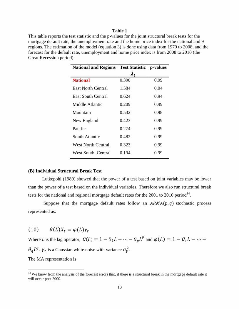
the results of the test together with the -values. The -value is the probability that the test

statistic assumes a value greater than the observed test value, if the null hypothesis is true. The

results show that with the exception of East North Central region there does not seem to be a

structural break in the underlying parameters for the other regions.

13

Pages 187-188 and Appendix C

13

Table 1

This table reports the test statistic and the p-values for the joint structural break tests for the

mortgage default rate, the unemployment rate and the home price index for the national and 9

regions. The estimation of the model (equation 3) is done using data from 1979 to 2008, and the

forecast for the default rate, unemployment and home price index is from 2008 to 2010 (the

Great Recession period).

(B) Individual Structural Break Test

Lutkepohl (1989) showed that the power of a test based on joint variables may be lower

than the power of a test based on the individual variables. Therefore we also run structural break

tests for the national and regional mortgage default rates for the 2001 to 2010 period14

.

Suppose that the mortgage default rates follow an ( ) stochastic process

represented as:

( ) ( ) ( )

Where is the lag operator, ( ) and ( )

. is a Gaussian white noise with variance

.

The MA representation is

14

We know from the analysis of the forecast errors that, if there is a structural break in the mortgage default rate it

will occur post 2000.

National and Regions

Test Statistic p-values

National

East North Central

East South Central

Middle Atlantic

Mountain

New England

Pacific

South Atlantic

West North Central

West South Central

0.390

1.584

0.624

0.209

0.532

0.423

0.274

0.482

0.323

0.194

0.99

0.04

0.94

0.99

0.98

0.99

0.99

0.99

0.99

0.99

14

( ) ( )

Where ( ) ( )

( ) ∑

A test statistic to test for a structural break is constructed as follows: Let the sum of

squared residuals of the estimation of Equation (11) using data from 1979 to 2007 be represented

as , and let the sum of squared residuals using data from 1979 to 2010 be

represented as . Then a test for structural break in the mortgage default rate from

2008 to 2010 is:

( ) [ ]

[ ] ( )

Where is the number of observations from 2008 to 2010, is the number of observations

from 1979 to 2007 and , the number of parameters to be estimated.

Table 2 presents the results of the structural break test together with the -values. The

results show that there has been a structural break in the national and regional mortgage default

rates during 2008 to 2010. This break in the mortgage default rates accounts for the huge

deviations in the forecast errors observed during the Great Recession (2008 to 2010). The SVAR

model using just estimates from fitting the model to the 1979 to 2000 sample to forecast the

mortgage default rates from 2001 to 2010 could not have anticipated this structural change. The

graphs of the national and regional mortgage default rates (Appendix D) show that there was not

much variation in the mortgage default rates until after 2007.

15

Table 2

This table reports the test statistic and the p-values for the individual structural break test for the

mortgage default rate of the national and 9 regions. The estimation of the model (Equation 11)15

is done using data from 1979 to 2010 and also data from 1979 to 2007.

5. Analysis of the Dynamics of the Unemployment and Home Price Index

shocks on the Mortgage Default Rate (National and Regional):

1979 to 2000 vs. 2001 to 2010

In this section we evaluate the impact of the home price index and unemployment shocks

on the mortgage default rates by examining the impulse response functions and the variance

decomposition from 1979 to 2000 and also from 2001 to 2010. Not only are we interested in the

dynamics of the two shocks on the mortgage default rates during both periods; we also want to

assess the relative importance of the shocks in explaining the variation in the mortgage default

rates.

5.1 Orthogonalized Impulse Response

An MA representation of equation (3) based on is given by:

15

The exact specification of the model for the national and the 9 regions are presented in Appendix C

National and Regions Test Statistic ( ) p-value

National

East North Central

East South Central

Middle Atlantic

Mountain

New England

Pacific

South Atlantic

West North Central

West South Central

8.431

11.439

30.078

27.557

7.104

18.327

8.124

17.479

4.050

18.344

0.000

0.000

0.000

0.000

0.000

0.000

0.000

0.000

0.011

0.000

16

( ) ∑

Where [

] ( ) The elements

of the matrices represent the responses to shocks.

5.2 Variance Decomposition

A variance decomposition is performed to measure the contribution of the home price

and unemployment shocks to the changes in default rates. Using equation (13), the error optimal

ahead forecast at time is:

( ) ∑

Denoting the element of by , then the forecast error of the

component of ( )becomes:

( ) ( ) ( ) ∑(

)

Thus the forecast error of the component consists of all the innovations:

and .

Because the are uncorrelated and have unit variances, the mean square error of ( )

can then be expressed as:

( ) ( ( ) ) ∑(

)

The contribution ( ) of the component to the MSE of the h-step ahead forecast of the

component is

17

( ) ( ) ∑

( )

This is the proportion of the forecast error variance error of variable

accounted for by

and innovations. We focus here on the proportion of the forecast

error variance of the mortgage default rate accounted by the unemployment and home price

index shocks.

5.3 Home Price Index and Unemployment Data: 2000 to 2010

The 2000 to 2010 period represents a time of significant changes in unemployment and

house prices. Table 3 presents the percentage appreciation and depreciation of the house price

index at the national and regional levels from 2000 to 2010.16

The table shows some variations

across the regions of the extent of house price appreciation and depreciation during this period.

House prices in the Pacific region had the largest appreciation and also the largest depreciation

during this period. There has not being significant house price depreciation in the West North

Central, West South Central and East South Central regions. The East North Central region had

the smallest house price appreciation but one of the largest house price depreciation. Housing

prices in New England and Middle Atlantic experienced large appreciation, but not significant

depreciation.

16

This period was chosen because it has the highest home price index and also the period when the index

depreciated (measuring from the peak value) the most. The window is wide enough to observe the scale of house

price appreciation for the regions and the subsequent collapse in house prices for some of the regions.

18

Table 3

This table reports the maximum House Price Index appreciation and the minimum House Price

Index depreciation from 1st quarter 2000 to 3

rd Quarter 2010

17.

National and Regions House Price Index

Appreciation %

House Price Index

Depreciation %

National

East North Central

East South Central

Middle Atlantic

Mountain

New England

Pacific

South Atlantic

West North Central

West South Central

66

33

43

87

76

82

124

83

45

47

-13

-11

-4

-9

-28

-12

-38

-18

-5

-2

Table 4 also reports the lowest and highest national and regional unemployment rates

during 2001 to 2010. The table shows that there were significant increases in the unemployment

rates both at the national and regional level during this period. East North Central and East South

Central regions have their highest unemployment rates above the highest national unemployment

rate. The two tables show that there were significant changes in house price indices and

unemployment rates during this period. This presents a perfect sample to test the relative

significance of home price index and unemployment shocks on the mortgage default rate.

17

National [Peak (1st qtr. 2007)]: ENC [Peak (1

st qtr. 2007): ESC [Peak (1

st qtr. 2008)]: MA [Peak (1

st qtr. 2007)]:

MT [Peak (2rd

qtr. 2007)]: NE [Peak (1st qtr. 2007): P [Peak (4

th qtr. 2006)]: SA [Peak (1

st qtr. 2007)]: WNC [Peak

(2nd

qtr. 2007)]: WSC [Peak (2nd

qtr. 2008)]. For the national and all the regions the minimum house price index

depreciation after the peak occurred during the 2nd

qtr. 2010.

19

Table 4

This table reports the lowest and highest national and regional unemployment rates 2001 to

2010. The dates for the lowest and highest values are provided in the brackets.

5.4 Impulse Response Functions

This section presents the results of the impulse response functions for the mortgage

default for the 1979 to 2000 and 2001 to 2010 samples.

Figures 5 to 8 represent the dynamics of the impulse response functions of the mortgage

default rates for the national, East South Central, West North Central and Middle Atlantic

regions18

respectively to an increase of one standard deviation in the home price index and the

unemployment rate. In response to the unemployment shocks, the national and regional mortgage

default rates increase and they take about 15 quarters after the shocks to get back to their pre

shock level. The home price shocks are unchanged in the period of impact because of our

identification scheme, which implied that it takes more than a quarter for the home price index

shocks to have an impact on the mortgage default rates. In response to the home price index

shocks the national and regional mortgage default rates decrease and they also take about 15

quarters to get back to its pre shock level. The national and regional mortgage default dynamics

after the shocks seem to be similar; however, there are regional variations in the peaks and

troughs of the impulse response functions.

18

The dynamics of the other regions are similar to those reported here.

National and Regions Lowest Unemployment rate Highest unemployment rate

National

East North Central

East South Central

Middle Atlantic

Mountain

New England

Pacific

South Atlantic

West North Central

West South Central

4.2 (1st qtr. 2001)

4.3 (1st qtr. 2001)

4.6 (1st qtr. 2001)

4.1 (1st qtr. 2001)

3.2 (1st qtr. 2007)

3.3 (1st qtr. 2001)

4.6 (1st qtr. 2007)

4.0 (2nd

qtr. 2006)

3.3 (1st qtr. 2001)

4.1 (1st qtr. 2008)

9.9 (4th

qtr. 2009)

11.1 (4th

qtr. 2009)

10.7 (4th

qtr. 2009)

9.1 (4th

qtr. 2009)

9.2 (1st qtr. 2010)

8.6 (4th

qtr. 2009)

9.7 (4th

qtr. 2009)

9.6 (4th

qtr. 2009)

6.5 (2nd

qtr. 2009)

7.7 (1st qtr. 2010)

20

Table 5 reports the peak and trough of the national and regional mortgage default rates

after the unemployment and home price index shocks. From 1979 to 2000 the national

unemployment and home price index shocks led to a maximum increase of 1.3% and a decrease

of 1% in the national mortgage default rates respectively. For the regions the unemployment and

home price index shocks led to an average increase of 1.2% and a decrease of 1.1% in the

regional mortgage default rate respectively. Compared to the 2001 to 2010 period, the national

unemployment and the home price index shocks led to maximum increase of 7.2% and a

decrease of 4.9% in the national mortgage default rate respectively. For the regions, the

unemployment and the home price index shocks led to an average increase of 12.7% and a

decrease of 7.3% respectively. Although there have been a lot of changes in the unemployment

rate at both the national and regional levels during the 1979 to 2000 period, these changes did not

seem to have impacted the national and regional mortgage default rates that much. The results

for the home price index during this period are not surprising because the indices did not change

much during the period.

For the 2001 to 2010 period, the unemployment results for the East South Central (which

had one of the highest unemployment rates at 11.1%) and West South Central (influenced by

Louisiana in particular) were mainly driven by the effects of hurricane Katrina. These two

regions were among the regions with the smallest house price index appreciation and

depreciation (Table 3); however the house price shocks seem to have generated a big impact on

the mortgage default rates.

Overall the response to the unemployment shocks is larger than the response to the home

price index shocks.

21

Table 5

This table reports the peak and trough of the impulse response functions of the national and

regional mortgage default rates due to a one standard deviation increase in the national and

regional unemployment rate and the national and regional home price indices.

National and

Regions

1979 to 2000 2001 to 2010

Unemployment Price Index Unemployment Price Index

% % % %

National

East North Central

East South Central

Middle Atlantic

Mountain

New England

Pacific

South Atlantic

West North Central

West South Central

1.3

1.9

1.4

1.1

1.0

1.2

0.6

0.7

1.4

1.4

-1.0

-1.5

-1.7

-0.2

-1.2

-1.1

-1.6

-1.0

-0.5

-1.5

7.2

11.4

18.0

6.9

10.4

8.4

5.9

9.1

5.4

39.0

-4.9

-6.0

-12.5

-5.1

-5.9

-5.6

-5.7

-7.8

-3.7

-8.7

22

Impulse Response Functions 1979 to 2000 vs. 2001 to 2010: National and Regional

23

5.5 Variance Decomposition

To gauge the relative contributions of the unemployment and the home price index

shocks to the variance of the mortgage default rates during both the 1979 to 2000 and the 2001 to

2010 periods; the variance decompositions are constructed for the SVAR system using Equation

(17) at ( ) and ( )19. Table 6 presents the results of the variance

decomposition. Again in this case also, the unemployment and home price index shocks do not

explain much of the variation in the forecast errors of the mortgage default rates at both the

national and regional levels for the 1979 to 2000 period. Although there are some regional

variations in the impact of the unemployment and home price index shocks during the 2001 to

2010 period, on average, employments shocks explain a larger percentage in the movement of

the mortgage default rates than the home price index shocks. The unemployment shocks explain

about 44% of the movement in the mortgage default rates at ( ) and 43%

( ). While the home price index shocks explains about 13% at ( ) and

20% ( ). In effect, the two shocks are responsible on average for about 60% of

the movement in the regional mortgage default rates.

The empirical results show that unemployment shocks have been a bigger contributor to

national and regional mortgage default rates than the home price index shocks.

19

As increases, the decomposition of the variance of the forecasting error coincides with the decomposition of the

unconditional variance.

24

Table 6

This table reports the variance decompositions, equation (17), of the national and regional

mortgage default rates for 1979 to 2000 and 2001 to 2010 samples for ( ) and ( ). The decompositions are expressed in percentages.

National and Regions 1979 to 2000 2001 to 2010

Unemployment Price Index Unemployment Price Index

National

East North Central

East South Central

Middle Atlantic

Mountain

New England

Pacific

South Atlantic

West North Central

West South Central

4.7 4.2

5.0 5.1

3.3 3.4

3.4 3.3

3.3 3.7

2.3 2.6

1.3 2.1

2.1 2.1

5.0 5.1

2.6 2.5

3.5 3.6

2.3 2.7

4.0 4.5

0.2 0.2

5.1 5.3

1.9 2.2

3.4 5.0

2.0 2.1

0.7 0.7

3.6 3.6

32 31

56 51

37 37

38 38

61 57

36 39

23 22

43 38

42 39

63 63

7 12

11 14

11 12

14 24

14 22

15 21

26 41

20 30

11 14

4 4

6. Dynamics of Some Selected States

The dynamics of the home price index and unemployment shocks on the mortgage

default rates were examined for Arizona, California, Florida, Michigan, Nevada, and

Pennsylvania. These states have had mortgage default rates higher than the national average.

Some of the states (Michigan, Nevada and Pennsylvania) have also had unemployment rates

higher than the national average. Arizona, California, Florida, Michigan and Nevada have also

experienced some of the biggest drop in housing prices during the 2001 to 2010 period.

6.1 Home Price Index and Unemployment Data: 2000 to 2010

From Table 7 Florida had the largest appreciation in the house price index from 2000 to

2010 and also one of the largest house price index depreciations during the period. Michigan had

one of the lowest appreciations in the house price index, but also one of the largest house price

index depreciation during the period. Nevada had the largest depreciation in the home price

25

index. Michigan had the smallest home price appreciation but a large home price index

depreciation. There does not seem to be have been much depreciation in housing prices in

Pennsylvania. Mayer and Pence (2009), document that areas with high house price appreciation

experienced an increase in subprime mortgage origination. Mayer et al (2009) also showed that

in California, Florida, Arizona and Nevada over half of subprime borrowers had negative equity

in their home and over a third of borrowers in Michigan had negative equity by mid-2008

Table 7

This table reports the maximum House Price Index appreciation and the minimum House Price

Index depreciation from 1st quarter 2000 to 3

rd Quarter 2010.

States House Price Index

Appreciation %

House Price Index

Depreciation %

Arizona

California

Florida

Michigan

Nevada

Pennsylvania

132

353

387

27

169

72

-36

-30

-36

-23

-45

-6

Table 8 also reports the lowest and highest state unemployment rates during this period.

The results show that there have been significant increases in the unemployment rates for these

states during this period. With the exception of Pennsylvania, all the states have their highest

unemployment rates above the highest national unemployment rate and also larger house price

index depreciation than the national. Again, these states present a perfect sample to test the

relative significance of home price index and unemployment shocks on the mortgage default

rate.

26

Table 8

This table reports the lowest and highest state unemployment rates 2001 to 2010. The dates for

the lowest and highest values are provided in the brackets.

6.2 Impulse Response Functions

This section presents the results of the impulse response functions for the mortgage

default for the 1979 to 2000 and 2001 to 2010 samples.

Figures 9 to 14 represents the dynamics of the impulse response functions of the

mortgage default rates for the states to an increase of one standard deviation in the home price

index and the unemployment rate. The dynamics of the states’ mortgage default rates after the

unemployment and home price shocks are similar to the dynamics of the national and regional

mortgage default rates after the shocks. That is, in response to the unemployment shocks the

states mortgage default rates increase and they take about 15 quarters after the shocks to get back

to its pre shock level. The home price shocks are also unchanged in the period of impact due to

the implication of our identification scheme. In response to the home price index shocks the

states mortgage default rates decrease and for some of the states it takes about 20 quarters to get

back to their pre shock level during the 2001 to 2010 period. However, for these selected states

the peak and trough of the impulse response functions are higher and lower for the

unemployment and home price index shocks respectively.

Table 5 reports the peak and trough of the state’s mortgage default rates after the

unemployment and home price index shocks. For the selected states also, there does not seem to

have been much of an impact on the mortgage default rates during the 1979 to 2000 period for

both the unemployment and home price shocks.

For the 2001 to 2010 period, the home price index shocks produced a larger impact on

the mortgage default rates of California and Florida than the unemployment shocks. For the other

National and Regions Lowest Unemployment rate Highest unemployment rate

Arizona

California

Florida

Michigan

Nevada

Pennsylvania

3.6 (2nd

qtr. 2007)

4.8 (3rd

qtr. 2006)

3.3 (2nd

qtr. 2006)

4.7 (1st qtr. 2001)

4.2 (4th

qtr. 2006)

4.2 (1st qtr. 2007)

10.4 (4th

qtr. 2009)

12.5 (3rd

qtr. 2010)

11.7 (3rd

qtr. 2010)

14.1 (3rd

qtr. 2009)

14.9 (3rd

qtr. 2010)

8..8 (1st qtr. 2010)

27

4 states the impact of the unemployment shocks was larger. For Nevada—which had the largest

home price depreciation and the highest unemployment rate during this period—the

unemployment shocks seem to have had a bigger impact on its mortgage default rates.

Table 9

This table reports the peak and trough of the impulse response functions of the state mortgage

default rates due to a one standard deviation increase in the state unemployment rate and the state

home price indices.

National and

Regions 1979 to 2000 2001 to 2010

Unemployment

%

Price Index

%

Unemployment

%

Price Index

%

Arizona

California

Florida

Michigan

Nevada

Pennsylvania

1.1

1.8

2.3

1.5

2.4

0.6

-1.2

-0.7

-0.8

-0.6

-0.6

-1.4

19.9

8.0

11.6

15.1

19.8

7.1

-12.0

-10.4

-14.8

-7.7

-11.4

-3.7

28

Impulse Response Functions 1979 to 2000 vs. 2001 to 2010: States

29

Impulse Response Functions 1979 to 2000 vs. 2001 to 2010: States

30

6.3 Variance Decomposition

The variance decomposition is performed for both the 1979 to 2000 and the 2001 to 2010

periods at ( ) and ( ). Table 10 presents the results. At the state

level also the unemployment and home price index shocks do not explain much of the variation

in the forecast errors of the mortgage default rate for the 1979 to 2000 period. During the 2001 to

2010 period, the unemployment shocks explained more of the variation in the mortgage defaults

rates than the home price index shocks at both the one and two year horizon. As Tables 7 and 8

shows, there have been significant changes in both the unemployment rates and the home price

indices, but the changes in the unemployment rate on average explained more of the variation in

the state mortgage default rates than the changes in the home price indices.

Policies that aim to decrease the default rates across the states should take into account

the relative impact of the two shocks in explaining the variation in the mortgage default rate. If

home price should dominate, then government programs that reduce the overall principal might

be beneficial for that state. By contrast, if unemployment shocks dominate, reduction in

payments (or subsidization mortgage payments) might be the better policy for the state.

Table 10

This table reports the variance decompositions, equation (17), of the states’ mortgage default

rates for 1979 to 2000 and 2001 to 2010 samples for ( ) and ( ). The decompositions are expressed in percentages.

States 1979 to 2000 2001 to 2010

Unemployment Price Unemployment Price

Arizona

California

Florida

Michigan

Nevada

Pennsylvania

1.5 1.5

7.0 7.3

7.6 7.9

3.1 3.2

4.8 5.1

1.8 1.8

2.7 3.6

0.8 0.9

0.9 1.2

0.4 0.4

0.5 0.6

1.3 1.3

53 57

17 14

27 26

62 60

54 43

40 37

19 18

21 38

28 32

10 12

10 22

4 9

31

7. Conclusion

The increase in mortgage default rates over the last several years has created a renewed

interest in the factors drive mortgage defaults. There has been an increase in the number of

subprime loans originated after 2003, due to lax mortgage underwriting standards. This has

increase the number of borrowers who are more susceptible to unemployment and negative home

price shocks. These borrowers have little savings they could use to cushion them against

unemployment and negative home price shocks. Studies have drawn conflicting conclusions as

to which of these two factors have accounted for the most of the variation in the mortgage

default rates. There is an important policy implications for how best to help home owners under

water depending on which factor dominates. As Elul et al (2010) stated if negative equity

dominates, then government programs that reduce the overall principal might be beneficial. By

contrast, if unemployment shocks should dominate, reduction in payments (or subsidization

mortgage payments) might be the better policy.

The paper uses an SVAR model to disentangle the interrelations between the home price

index (which tracks housing prices) and unemployment shocks and mortgage default rates by

studying the dynamics of these two shocks on mortgage default rates from 1979 to 2010 at the

national, regional and state levels. The results show that, with the exception of the Pacific region,

California and Florida, unemployment shocks explain more of the variation in the mortgage

default rates than home price indices shock at the national, regional and state levels, especially,

during the 2001 to 2010 period. These two shocks together are responsible on average for about

60% of the movement in the regional mortgage default rates.

32

References

Ambrose, Brent W., Charles A. Capone, and Yongheng Deng, 2001, “Optimal Put Exercise:

An Empirical Examination of Conditions for Mortgage Foreclosure” Journal of Real Estate

Finance and Economics, 23(2): 213-34.

Ang, Andrew and Monika Piazzesi, 2003, "A No-Arbitrage Vector Autoregression of Term

Structure Dynamics with Macroeconomic and Latent Variables", Journal of Monetary

Economics, 50, 4, 745-787.

Ashworth, Roger, Laurie Goodman. Brian Landy and Ke Yin, 2010, “Negative Equity Trumps

Unemployment in Predicting Defaults” The Journal of Fixed Income, 19(4), 67-72

Clauretie, Terrence M., 1987, “The Impact of Interregion Foreclosure Cost Differences and the

Value of Mortgages on Default Rates” American Real Estate and Urban Economics

Association Journal, 15(3): 152-67.

Bhutta, Neil, Jane Dokko, and Hui Shan. 2010. “How Low Will You Go? The Depth of Negative

Equity and Mortgage Default Decisions” Unpublished.

Christiano, Lawrence and Evans Eichenbaum, 1999, “Monetary Policy Shocks: What Have we

Learned and to What End?” Handbook of Macroeconomics eds Woodford, M., Taylor, J. (North

Holland, Amsterdam).

Demyanyk, Yuliya and Otto Van Hemert, (2008), “Understanding the Subprime Mortgage

Crises” Review of Financial Studies, 24(6), 1848-1880

Deng, Yongheng, John M. Quigley, and Robert Van Order, 2000, “Mortgage Terminations,

Heterogeneity and the Exercise of Mortgage Options” Econometrica, 68(2), 275-307

Elul, Ronel, Souphala Chomsisengphet, Dennis Glennon, and Robert Hunt and Nicholas S.

Souleles, 2010, “What “Triggers” Mortgage Default?” American Economic Review: Papers &

Proceedings, 100: 490–494

Foote, Christopher, Kristopher Gerardi, Lorenz Goette, and Paul Willen, 2009,” Reducing

Foreclosures: No Easy Answers” Federal Reserve Bank of Atlanta, Working Paper 2009-15

Foster, Chester, and Robert Van Order, 1984, “An Option-based Model of Mortgage Default.”

Housing Finance Review, 3(4): 351–72

Ghent, Andra and Marianna Kudlyaky, 2009, “Recourse and Residential Mortgage Default:

Theory and Evidence from U.S. Regions” Federal Reserve Bank of Richmond, Working Paper

No. 09-10

Jones, Lawrence D., 1993, “Deficiency Judgments and the Exercise of the Default Option in

Home Mortgage Loans” Journal of Law and Economics, 36(1): 115-38.

33

Kau, James, Donald Keenan, and Taewon Kim. 1994. “Default Probabilities for

Mortgages,” Journal of Urban Economics, 35(3), 278-296.

Keys, Benjamin, Timothey Mukherjee, Amit Seru and Vikrant Vig, 2008, “Did Securitization

Lead to Lax Screening? Evidence from Subprime Loans, 2001-2006” Quarterly Journal of

Economics, 125(1), 307-362.

Lutkepohl, Helmut, 2005, “New introduction to Multiple Time Series Analysis” Springer

Lutkepohl, Helmut, (1989), “Prediction Tests for Structural Stability of Multiple Time Series”

Journal of Business & Economic Statistics, 7, 129-135.

Mayer, Christopher and Karen Pence, 2009, “Subprime Mortgages: What, Where, and to

Whom?” In Edward L. Glaeser and John M. Qugley, eds. Housing Markets and the Economy:

Risk, Regulation, and Policy. Cambridge, MA: Lincoln Institute of Land Policy.

Mayer, Christopher, Karen Pence and Shane Sherlund, 2009, “The Rise in Mortgage default”

Journal of Economic Perspective, 23(1), 27-50

Mian, Atif and Amir Sufi, 2009, “The Consequences of Mortgage Credit Expansion: Evidence

from the U.S. Mortgage Default Crises” Quarterly Journal of Economics, 124(4), 1449-1496

Mian, Atif and Amir Sufi, 2011, “House Prices, Home Equity-Based Borrowing, and the U.S.

Household Leverage Crises” American Economic Review, 101, 2132-2156

Mian, Atif , Amir Sufi and Francesco Trebbi , 2010, “The Political Economy of the U.S.

Mortgage Default Crises” American Economic Review, 67-98

Mian, Atif, Amir Sufi and Francesco Trebbi, 2012, “Foreclosures, House Prices, and the Real

Economy” Working Paper, May

Saiz, Albert, 2010, "The Geographic Determinants of Housing Supply;" Quarterly Journal of

Economics. 125(3), 1253-1296.

StataCorp, 2011, Time Series Reference Manual, College Station, TX: StataCorp LP.

Uribe, Martin and Vivian Yue, 2006, “Country Spreads and Emerging Countries: Who Drives

Whom,” Journal of International Economics?” 69, 6-36.

Vandell, Kerry, 1978, “Default Risk Under Alternative Mortgage Instruments” The

Journal of Finance, 33(5), 1279-1296.

34

Appendix A (Regions: US Census Bureau)

East North Central: Michigan, Wisconsin, Illinois, Indiana, Ohio

East South Central: Kentucky, Tennessee, Mississippi, Alabama

Middle Atlantic: New York, New Jersey, Pennsylvania

Mountain Census Division: Montana, Idaho, Wyoming, Nevada, Utah, Colorado, Arizona, New

Mexico

New England: Maine, New Hampshire, Vermont, Massachusetts, Rhode Island, Connecticut

Pacific Census Division: Hawaii, Alaska, Washington, Oregon, California

South Atlantic: Delaware, Maryland, District of Columbia, Virginia, West Virginia,

North Carolina, South Carolina, Georgia, Florida

West North Central: North Dakota, South Dakota, Minnesota, Nebraska, Iowa, Kansas,

Missouri

West South Central: Oklahoma, Arkansas, Texas, Louisiana

35

Appendix B

Forecasting with Estimated Process

From Lutkepohl (2005), if we denote the parameter estimators of the SVAR system, Equation

(3), as ... and

The asymptotic estimator of the covariance matrix of the prediction error is given by:

( ) ( ) ( )

( )

Where

( ) ( ) {[ ( )][ ( )] } ∑

And is the coefficient of the canonical MA representation of , Equation (13).

( ) ( )

∑{∑

( )

}

{∑ ( )

}

[

]

(

)

∑

36

is the estimate of the covariance matrix of the innovations and is the covariance matrix

of the asymptotic distribution of √ ( ).

For a simulation with R repetitions, this algorithm is used20

:

1. Fit the model and save the estimated coefficients. Only data up to T is used for the estimation.

2. Use the estimated coefficients to calculate the residuals.

3. Repeat steps 3a–3c R times.

3a. Draw a simple random sample with replacement of size T +h from the residuals.

When the th observation is drawn, all K residuals are selected, preserving any contemporaneous

correlation among the residuals.

3b. Use the sampled residuals, p initial values of the endogenous variables, any

exogenous variables, and the estimated coefficients to construct a new sample dataset.

3c. Save the simulated endogenous variables for the h forecast periods in the

bootstrapped dataset.

20

StataCorp, 2011, Time Series Reference Manual p. 151

37

Appendix C Individual structural test

Table C.1 This table reports the optimal lag for estimating equation (16) for the full sample (1979 to 2010)

and the 1979 to 2007 sample. Akaike's information criterion (AIC) was used in selecting the

optimal lags

National and Regions

ARMA Degrees of Freedom

National (6,2) F(11,107)

East North Central (4,2) F(11,109)

East South Central (6,2) F(11,107)

Middle Atlantic (3,2) F(11,110)

Mountain (4,2) F(11,109)

New England (3,1) F(11,111)

Pacific (5,2) F(11,108)

South Atlantic (2,2) F(11,111)

West North Central (5,2) F(11,108)

West South Central (3,2) F(11,110)

38

Appendix D Graphs of National and Regional Mortgage Default Rate

39