Dynamics of Target-Mediated Drug Disposition

A Mathematical Analysis

Lambertus A. Peletier & Johan Gabrielsson

Warwick - March 27, 2014

Outline

1. Analysis of data sets - Characteristic patterns

2. Simulations of the TMDD model

3. Identification of di↵erent phases of the dynamics

4. Obtaining quantitative results - Parameter estimates

5. Simplified models

Warwick, 14-03-27 1

– Typeset by FoilTE

X – 1

Linear pharmacokinetics

One-compartment model:

VpdCp

dt= Input� Cl Cp, Vp = Plasma volume.

Two-compartment model:8>><

>>:

VpdCp

dt= Input� ClpCp � Cld(Cp � Ct),

VtdCt

dt= Cld(Cp � Ct),

(Cld � Clp)

0 10 20 30 40 5010−2

10−1

100

Time (t)

log{

Cp(t)

}

1 Compartment model2 Compartment model

Warwick, 14-03-27 2

– Typeset by FoilTE

X – 2

Nonlinear pharmacokinetics

0.01

0.1

1

10

100

1000

0 5 10 15 20 25 30 35 40 45

Time (days)

Concen

tration (

mg·L

-1)

InL

Michaelis-Menten(L)

Cld CP, VcCt, Vt

Linear ClEH

Data and fit of the concentration of the antibody hu1124 in humans withPsoriasis (a chronic skin disease) from Bauer et. al. (1999), using:

8>><

>>:

VcdCp

dt= �ClEHCp � Cld(Cp � Ct)�V

max

Cp

Km + Cp

VtdCt

dt= Cld(Cp � Ct)

Empirical evidence: Saturable elimination: Michaelis-Menten elimination

Find: A mechanistic explanation

Warwick, 14-03-27 3

– Typeset by FoilTE

X – 3

Another data set

Gabrielsson & Peletier TMDD2 2011

3

CL 0.001 1 KON 0.099 17 KOFF 0.001 27 VT 0.101 2 CLD 0.003 4 KOUT 0.009 6 R0 12. 4 KERL 0.002 27

0.001

0.01

0.1

1

10

100

1000

0 100 200 300 400 500 600 Time (h)

Con

cent

ratio

n (..

)

Two points of inflection!

Warwick, 14-03-27 4

– Typeset by FoilTE

X – 4

Target-Mediated Drug Disposition

Ligand and Receptor (Target) form active complex

RL + RL

kin

kout

kon

koffke(RL)

InL

L = Ligand

R = receptor

RL = Receptor-Ligand

complex ke(L)

Parameter fit

kon

ko↵

kin

kout

ke(L)

ke(RL)

R0

=

kin

kout

0.091 0.001 0.11 0.0089 0.0015 0.003 12.36(mg/L)�1h�1 h�1 (mg/L) h�1 h�1 h�1 h�1 mg/L

Kddef

=

ko↵

kon

= 0.011 mg/L & Kmdef

=

ko↵

+ ke(RL)

kon

= 0.044 mg/L

Warwick, 14-03-27 5

– Typeset by FoilTE

X – 5

Questions

1. How to estimate the six parameters?

2. Which data do you need:

• Is data about ligand L enough?

• Data about target R and complex RL?

Often di�cult, if not impossible, to get.

3. Over what period do you need data? (Design of experiments)

4. How to distinguish between empirical Michaelis-Menten and TMDD?

5. Validity of Rapid Binding and Quasi-Steady-State models.

Warwick, 14-03-27 6

– Typeset by FoilTE

X – 6

The equations

The dynamics is given by the system of nonlinear di↵erential equations:

8>>>>>><

>>>>>>:

dL

dt= InL � k

on

L ·R+ ko↵

RL � ke(L)

L

dR

dt= k

in

� kout

R � kon

L ·R+ ko↵

RL

dRL

dt= k

on

L ·R� ko↵

RL � ke(RL)

RL

If InL = 0, then the Baseline is given by

L = 0, R = R0

def

=

kin

kout

, RL = 0.

The initial concentrations, right after a bolus dose, are given by

L(0) = L0

, R(0) = R0

, RL(0) = 0.

Warwick, 14-03-27 7

– Typeset by FoilTE

X – 7

Simulations - Linear scale

0 500 1000 1500 2000 2500

100200300400500600700800900

1000

Time (h)

L

L0 = 30, 100, 300, 900; R0=12

0 500 1000 1500 2000 25000

5

10

15

20

25

30

35

40

Time (h)

R

L0 = 30, 100, 300, 900; R0=12

0 500 1000 1500 2000 2500

5

10

15

20

25

30

35

40

Time (h)

RL

L0 = 30, 100, 300, 900; R0=12

0 500 1000 1500 2000 25000

5

10

15

20

25

30

35

40

Time (h)

R+R

L

L0 = 30, 100, 300, 900; R0=12

Warwick, 14-03-27 8

– Typeset by FoilTE

X – 8

Simulations - Logarithmic scale

0 500 1000 1500 2000 250010−4

10−2

100

102

104

Time (h)

Liga

nd (m

g/L) R0

Kd

0 1000 2000 3000 4000 500010−6

10−4

10−2

100

102

Time (h)

Log(

R0−

R)

L0 = 30, 100, 300, 900; R0=12

0 2000 4000 6000 800010−6

10−4

10−2

100

102

Time (h)

Log(

RL)

L0 = 30, 100, 300, 900; R0=12

0 2000 4000 6000 800010−6

10−4

10−2

100

102

Time (h)

Log(

R+R

L−R

0)

L0 = 30, 100, 300, 900; R0=12

Warwick, 14-03-27 9

– Typeset by FoilTE

X – 9

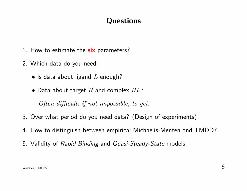
Characteristics of the Ligand versus time graph

Con

cent

ratio

n

Time

Rapid 2-order decline

Slow 1-order disposition Target route saturated

Mixed-order disposition Target route still partly saturated

koff- and kint-driven disposition Target Mediated Drug Disposition

Phase A: L, R and RL (quickly) reach quasi-equilibrium (0 < t < T1

)

Phase B: Target is saturated - linear (T1

< t < T2

)

Phase C: L = O(Km); target unsaturated - nonlinear (T2

< t < T3

)

Phase D: Linear elimination. (T3

< t < 1)

Warwick, 14-03-27 10

– Typeset by FoilTE

X – 10

Phase A: Short time dynamics

0 1 2 3 4 50

5

10

15

Time (h)

D0−

L (m

g/L)

0 1 2 3 4 50

5

10

15

Time (h)R

(m

g/L)

L0=30

L0=100

L0=300

L0=900

R0=12

0 1 2 3 4 50

5

10

15

Time (h)

RL

(mg/

L)

Conservation laws for L and R:

Ltot

= L+RL Rtot

= R+RL

8>><

>>:

dLtot

dt� ke(L)

L� ke(RL)

RL

dRtot

dt= k

in

� kout

R� ke(RL)

RL

Warwick, 14-03-27 11

– Typeset by FoilTE

X – 11

Dimensionless variables

In order to compare the magnitude of the di↵erent terms in the system ofdi↵erential equations we introduce dimensionless variables.

(1) Scale the concentrations with appropriate reference values:

x =

L

L0

, y =

R

R0

, z =

RL

R0

(2) Scale the time with an appropriate time scale. Consider the equation:

dL

dt= �k

on

L ·R =) dx

dt= �k

on

R0

x · y

This suggests for dimensionless time ⌧ :

⌧ = kon

R0

t (or ⌧ = kon

L0

t)

Warwick, 14-03-27 12

– Typeset by FoilTE

X – 12

Dimensionless equations

Introducing the dimensionless variables leads to the equations8>>>>>>><

>>>>>>>:

dx

d⌧= �x · y + µ

Kd

R0

z � kel

kon

R0

x

dy

d⌧=

kout

kon

R0

(1� y)�1

µx · y + Kd

R0

z

dz

d⌧=

1

µx · y � Kd

R0

z �ke(RL)

kon

R0

z

µ =

R0

L0

For the conservation laws we obtain:8>>><

>>>:

d

d⌧(x+ µz) = �"

✓kel

ko↵

x+ µke(RL)

ko↵

z

◆

d

d⌧(y + z) = "

✓kout

ko↵

(1� y)�ke(RL)

ko↵

z

◆ " =Kd

R0

⇡ 10

�3

Because " ⌧ 1 we conclude that

x(⌧) + µz(⌧) ⇡ 1, y(⌧) + z(⌧) ⇡ 1

Warwick, 14-03-27 13

– Typeset by FoilTE

X – 13

Phase A: Short-time dynamics

Elimination of x and y yields:

µdz

d⌧= f(z)

def

= (1� µz)(1� z)

⇢�µ

Km

R0

�

Note that µKm

R0

= O(µ · ") and may be omitted.0 1 2 3

−0.5

0

0.5

1

1.5

z

f(z)

Exercise 1: The function f(z) has a unique zero z = 1 in the interval[0, 1], and that

(a) z(⌧) ! z as ⌧ ! 1;

(b) ⌧1/2 = O

✓1

µ

◆, t

1/2 = O

✓1

kon

L0

◆(if µ ⌧ 1)

Exercise 2: Show that

L(t) ! L = L0

�R0

R(t) ! 0, RL(t) ! R0

as t ! T1

Warwick, 14-03-27 14

– Typeset by FoilTE

X – 14

Receptor dynamics

Recall thatdR

tot

dt= k

in

� kout

R� ke(RL)

RL

Rtot

= R+RLand initially

R(0) = R0

and RL(0) = 0

Then the following uniform upper bound holds:

Theorem 1: Let R, RL and Rtot

satisfy the above equations. Then

Rtot

(t) max

⇢kin

kout

,kin

ke(RL)

�for all t � 0

These bounds are valid for all L0

> 0, and all parameter values.

Exercise 3: Prove this theorem.

Warwick, 14-03-27 15

– Typeset by FoilTE

X – 15

Receptor dynamics in Phase B (L � Km)

In Phase B: L, R and RL are approximately in quasi-equilibrium:

RL ⇡ Rtot

L

L+Kmand R ⇡ R

tot

Km

L+Km

Hence, since in Phase B we have L � Km, it follows that

RL ⇡ Rtot

and R ⇡ 0

ThereforedR

tot

dt= k

in

� ke(RL)

Rtot

, T1

< t < T2

Since T1

⇡ 0 =) Rtot

(T1

) ⇡ R0

, we obtain for 0 < t < T1

,

Rtot

(t) ⇡ R⇤ + (R0

�R⇤)e�ke(RL)

t, R⇤ =kin

ke(RL)

Warwick, 14-03-27 16

– Typeset by FoilTE

X – 16

Receptor curve in Phase B - theory and simulation

0 500 1000 1500 2000 25000

5

10

15

20

25

30

35

40

Time (h)

Rto

t = R

+ R

L

L0 = 30, 100, 300, 900; R0=12

Rtot

(t) ⇡ R⇤ + (R0

�R⇤)e�ke(RL)

t, 0 < t < T2

t1/2 =

ln(2)

ke(RL)

= 231 h

Warwick, 14-03-27 17

– Typeset by FoilTE

X – 17

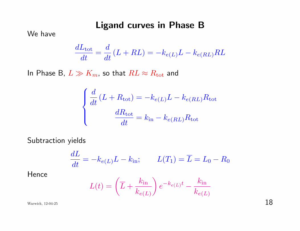
Ligand curves in Phase BWe have

dLtot

dt=

d

dt(L+RL) = �ke(L)

L� ke(RL)

RL

In Phase B, L � Km, so that RL ⇡ Rtot

and

8>><

>>:

d

dt(L+R

tot

) = �ke(L)

L� ke(RL)

Rtot

dRtot

dt= k

in

� ke(RL)

Rtot

Subtraction yields

dL

dt= �ke(L)

L� kin

; L(T1

) = L = L0

�R0

Hence

L(t) =

✓L+

kin

ke(L)

◆e�ke(L)

t � kin

ke(L)

Warwick, 12-04-25 18

– Typeset by FoilTE

X – 18

Ligand curve in Phase B - simulation

0 500 1000 1500 2000 250010−4

10−2

100

102

104

Time (h)

Rto

t = R

+ R

L

L0 = 30, 100, 300, 900; R0=12

R0

10 x Km

Km

L(t) =

✓L+

kin

ke(L)

◆e�ke(L)

t � kin

ke(L)

, L = L0

�R0

Warwick, 14-03-27 19

– Typeset by FoilTE

X – 19

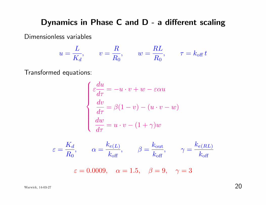
Dynamics in Phase C and D - a di↵erent scaling

Dimensionless variables

u =

L

Kd, v =

R

R0

, w =

RL

R0

, ⌧ = ko↵

t

Transformed equations:8>>>>>><

>>>>>>:

"du

d⌧= �u · v + w � "↵u

dv

d⌧= �(1� v)� (u · v � w)

dw

d⌧= u · v � (1 + �)w

" =Kd

R0

, ↵ =

ke(L)

ko↵

, � =

kout

ko↵

, � =

ke(RL)

ko↵

" = 0.0009, ↵ = 1.5, � = 9, � = 3

Warwick, 14-03-27 20

– Typeset by FoilTE

X – 20

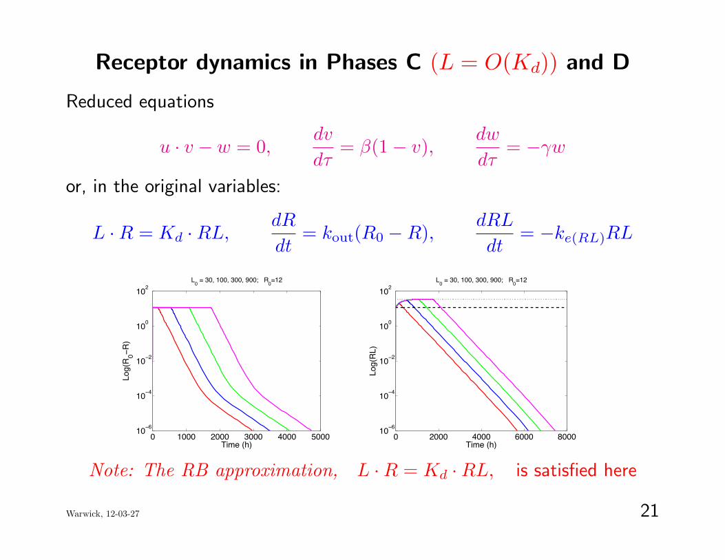
Receptor dynamics in Phases C (L = O(Kd)) and D

Reduced equations

u · v � w = 0,dv

d⌧= �(1� v),

dw

d⌧= ��w

or, in the original variables:

L ·R = Kd ·RL,dR

dt= k

out

(R0

�R),dRL

dt= �ke(RL)

RL

0 1000 2000 3000 4000 500010−6

10−4

10−2

100

102

Time (h)

Log(

R0−

R)

L0 = 30, 100, 300, 900; R0=12

0 2000 4000 6000 800010−6

10−4

10−2

100

102

Time (h)

Log(

RL)

L0 = 30, 100, 300, 900; R0=12

Note: The RB approximation, L ·R = Kd ·RL, is satisfied here

Warwick, 12-03-27 21

– Typeset by FoilTE

X – 21

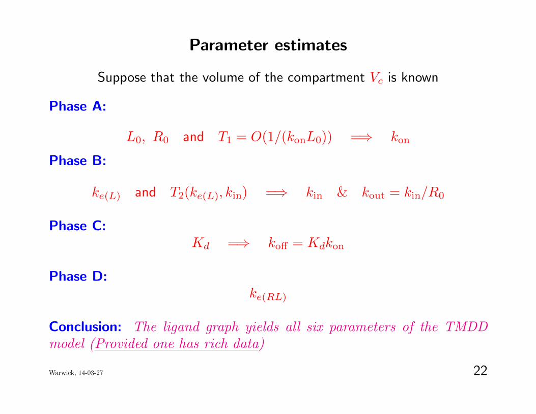
Parameter estimates

Suppose that the volume of the compartment Vc is known

Phase A:

L0

, R0

and T1

= O(1/(kon

L0

)) =) kon

Phase B:

ke(L)

and T2

(ke(L)

, kin

) =) kin

& kout

= kin

/R0

Phase C:Kd =) k

o↵

= Kdkon

Phase D:ke(RL)

Conclusion: The ligand graph yields all six parameters of the TMDDmodel (Provided one has rich data)

Warwick, 14-03-27 22

– Typeset by FoilTE

X – 22

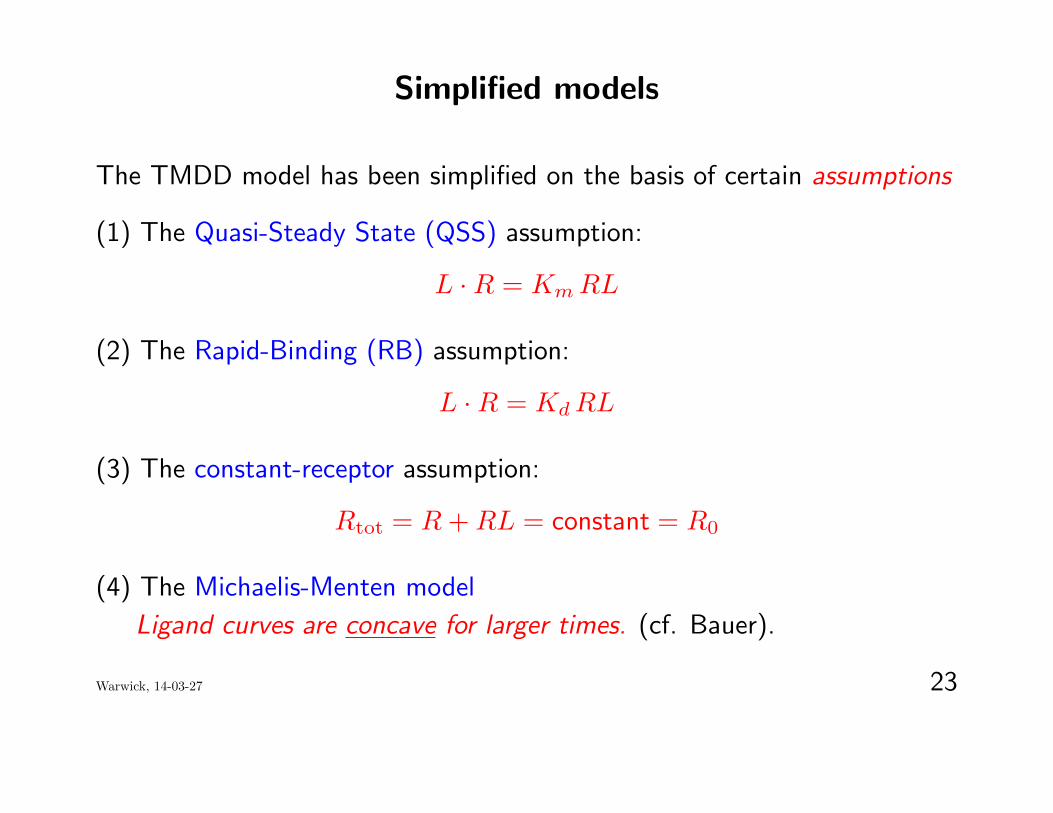
Simplified models

The TMDD model has been simplified on the basis of certain assumptions

(1) The Quasi-Steady State (QSS) assumption:

L ·R = KmRL

(2) The Rapid-Binding (RB) assumption:

L ·R = KdRL

(3) The constant-receptor assumption:

Rtot

= R+RL = constant = R0

(4) The Michaelis-Menten model

Ligand curves are concave for larger times. (cf. Bauer).

Warwick, 14-03-27 23

– Typeset by FoilTE

X – 23

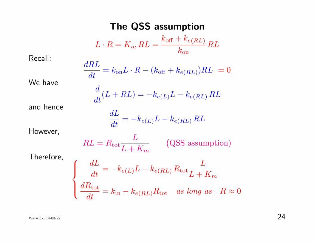
The QSS assumption

L ·R = KmRL =

ko↵

+ ke(RL)

kon

RL

Recall:dRL

dt= k

on

L ·R� (ko↵

+ ke(RL)

)RL = 0

We haved

dt(L+RL) = �ke(L)

L� ke(RL)

RL

and hencedL

dt= �ke(L)

L� ke(RL)

RL

However,

RL = Rtot

L

L+Km(QSS assumption)

Therefore, 8>><

>>:

dL

dt= �ke(L)

L� ke(RL)

Rtot

L

L+Km

dRtot

dt= k

in

� ke(RL)

Rtot

as long as R ⇡ 0

Warwick, 14-03-27 24

– Typeset by FoilTE

X – 24

The constant receptor assumption

kout

= ke(RL)

=) R+RL ⌘ R0

The QSS model now simplifies to the MM model:

dL

dt= �ke(L)

L� ke(RL)

R0

L

L+Km

The Full model simplifies to8>><

>>:

dL

dt= �(k

on

R0

+ ke(L)

)L+ (kon

L+ ko↵

)RL

dRL

dt= k

on

R0

L� (kon

L+ ko↵

+ ke(RL)

)RL

The dashed lines are the Null clines on which dRL/dt = 0 and dL/dt = 0:

RL = R0

L

L+Km, RL = R

0

L+ e(L)

L+Kd, e(L)

=

ke(L)

kon

0 10 20 300

5

10

15

L

RL

0 0.5 1 1.5 2 2.50

5

10

15

L

RL

Warwick, 14-03-27 25

– Typeset by FoilTE

X – 25

Conclusions

1. It is possible to extract the following information from ligand-versus timecurves over a su�ciently long time span:

(a) Estimates for many parameters.

(b) Analytical approximations over the time span when L � Km.

(c) Estimates for the Area Under the ligand-versus-time curve and Clearancewhen L

0

� Km.

2. Verifying the assumptions under which simplified models are valid is achallenge.

3. The Michaelis-Menten model cannot fit ligand-versus-time curves with morethan 1 inflection point.

Warwick, 14-03-27 26

– Typeset by FoilTE

X – 26

References

Gibiansky L, Gibiansky E, Kakkar T, Ma P (2008) Approximations of the target-mediated drug disposition model and identifiability of model parameters. J PharmacokinetPharmacodyn 35(5):573-591

Ma P (2012) Theoretical considerations of target-mediated drug disposition models:simplifications and approximations. Pharm Res 29:866-882

Mager DE, Jusko WJ (2001) General pharmacokinetic model for drugs exhibiting target-mediated drug disposition. J Pharmacokinet Pharmacodyn 28(6):507-532

Mager DE, Krzyzanski W (2005) Quasi-equilibrium pharmaco- kinetic model for drugsexhibiting target-mediated drug disposition. Pharm Res 22(10):1589-1596

Peletier LA, Gabrielsson J (2009) Dynamics of target-mediated drug disposition. Eur JPharm Sci 38:445-464

Peletier LA, Gabrielsson J (2012) Dynamics of target-mediated drug disposition:characteristic profiles and parameter identification, J Pharmacokinet Pharmacodyn 39:429-451

Warwick, 14-03-27 27

– Typeset by FoilTE

X – 27