Shocks in food availability and intra-household resources ...
Upload
hoangquynhCategory
view
216download
0
Hitotsubashi University Repository
Title
Dynamics of Household Assets and Income Shocks in
the Long-run Process of Economic Development The
Case of Rural Pakistan
Author(s) Kurosaki Takashi
Citation
Issue Date 2013-04
Type Technical Report
Text Version publisher
URL httphdlhandlenet1008625598
Right
PRIMCED Discussion Paper Series No 39
Dynamics of Household Assets and Income Shocks in
the Long-run Process of Economic Development The
Case of Rural Pakistan
Takashi Kurosaki
March 2013
Research Project PRIMCED Institute of Economic Research
Hitotsubashi University 2-1 Naka Kunitatchi Tokyo 186-8601 Japan
httpwwwierhit-uacjpprimcede-indexhtml
Dynamics of Household Assets and Income Shocks in the Long-run Process of
Economic Development The Case of Rural Pakistan
This version April 30 2013
(Previous versions April 15 2013 March 17 2013)
Takashi Kurosaki
Abstract
In this paper we analyze the dynamics of assets held by low-income households facing various types of income shocks in pre- and post-independence Pakistan Focusing on the province of Khyber Pakhtunkhwa (formerly known as the North-West Frontier Province NWFP) we first investigate the long-run data at the district level beginning from 1902 The results show that the population of livestock the major asset of rural households experienced a persistent decline after crop shocks due to droughts but did not respond much to the Great Depression In the post-independence period crop agriculture continued to be vulnerable to natural disasters although less substantially while the response of livestock to such shocks was indiscernible from district-level data To examine microeconomic mechanisms underlying such asset dynamics we analyze a panel dataset collected from approximately 300 households in three villages in the NWFP during the late 1990s The results show that the dynamics of household landholding and livestock is associated with a single long-run equilibrium When human capital is included the dynamics curve changes its shape but is not sufficiently nonlinear to produce statistically significant multiple equilibriums The size of livestock holding was reduced in all villages hit by macroeconomic stagnation while land depletion was reported only in a village with inferior access to markets The patterns of asset dynamics ascertained from historical and contemporary analyses are consistent with limited but improving access to consumption smoothing measures in the study region over the century
JEL classification codes O13 O44 N55
Keywords asset dynamics natural disaster buffer stock poverty trap Pakistan
The author would like to thank Natalie Chun S Hirashima Charles Horioka Masahiro Kawai Yukinobu Kitamura Motoi Kusadokoro Ken Miura Tetsuji Okazaki Hiroshi Sato Masahiro Shoji Koji Yamazaki and Yoshifumi Usami for their productive comments on the earlier versions of this paper The author is also grateful for their useful comments to other participants at the 2012 Asian Historical Economics Conference (Tokyo September 2012) the Asian Development Review Conference on Development Issues in Asia (Manila November 2012) and the Kansai Research Group on Development Microeconomcis (Osaka April 2013) All remaining errors are the authorrsquos This paper has been funded by a JSPS Grant-in-Aid for Scientific Research-S (22223003) Institute of Economic Research Hitotsubashi University 2-1 Naka Kunitachi Tokyo 186-8603 Japan Phone +81-42-580-8363 Fax +81-42-580-8333 E-mail kurosakiierhit-uacjp
11
1 Introduction
Natural and manmade disasters such as floods droughts earthquakes depressions
hyperinflation epidemics etc have affected the local and household economy worldwide and
throughout modern history Households in contemporary low-income developing countries are
particularly vulnerable for several reasons First their initial welfare levels are already close to
the poverty line Second institutional arrangements to cope with disasters are lacking Third
early warning systems are absent Similar reasons are applicable to households in developed
countries before the countries experienced modern economic growth This is because of the
presence of numerous symptoms associated with absolute poverty in such economies To
compound issues according to the emergency events database (EM-DAT) there appears to be
an increase in the number of natural disasters globallymdashfrom fewer than 100 per year in the
mid-1970s to approximately 400 per year during the 2000s1
Thus it is of critical importance to understand how households are affected by such
disasters how they recover from them and how policies and market environments affect the
dynamic process of recovery in the context of long-run economic development Under
incomplete markets particularly with underdeveloped credit markets and missing insurance
markets poor households need to save as a precaution against downturn risk such as natural and
manmade disasters As a result the asset choices of poor households may be excessively
sensitive to risk avoidance thereby causing them to miss the opportunity to enhance expected
income In development economics there are numerous theoretical and empirical studies that
focus on householdsrsquo ability to cope with these shocks (Fafchamps 2003 Dercon 2005)
Furthermore if the asset dynamics is highly nonlinear associated with low and high long-run
equilibriums farmers may reduce consumption substantially after a disaster to preserve the asset
and avoid a low equilibrium (Carter and Barrett 2006) In an extreme case households may
find themselves in a poverty trap in the aftermath of disasters These theoretical predictions
have been investigated quantitatively for several developing countries but there is no consensus
regarding the shape of the asset dynamics curve2 Among recent studies McKay and Perge
(2011) tested for evidence of the existence of an asset-based poverty trap mechanism across
seven panel datasets in developing countries however they did not find evidence for this
mechanism
In contrast the number of quantitative analyses on asset dynamics applied to historical
contexts is small mostly due to the nonavailability of suitable data As an exception the case of
1Available on httpwwwemdatbenatural-disasters-trends (accessed on October 20 2012) It is possible that the reported increase is partially due to an increased tendency to report not necessarily an increase in the occurrence of disasters 2For example see Naschold (2005) Adato et al (2006) Carter et al (2007) Mogues (2011) McKay and Perge (2011) and Miura et al (2012)
22
prewar Japanese farmers has been analyzed in several studies For example Kusadokoro et al
(2012) analyzed the asset accumulation behavior of farm households in rural Japan using panel
data from 1931 to 1941 the years of reconstruction following the Great Depression They
showed that households accumulated liquid assets such as cash quasi-money livestock animals
and in-kind stocks thereby suggesting the existence of a precautionary saving motive
Analyzing the same period but with a different data source Fujie and Senda (2011) showed that
farm households maintained the amount of arable land increased the nonfarm labor supply and
decreased the use of fertilizer in response to the depression They indicated that the aggregate
shocks from the Great Depression led to the stagnation of agricultural growth in Japan Both
these studies applied microeconometric approaches similar to those reviewed in the previous
paragraph Since the data requirement is high application of these approaches to other historical
cases is not straightforward
In this paper we attempt to fill these gaps in the literature by combining empirical
analyses using long-run historical data at the macro or semi-macro levels and contemporary data
collected at the household level This analysis focuses on the province of Khyber Pakhtunkhwa
(formerly known as the North-West Frontier Province the NWFP)3 Pakistan Using these
different data sources we address the question of how assetsmdashparticularly livestock which is
the core asset in the study areamdashrespond to natural and manmade disasters
We use long-run historical (semi-) macro data combined with data from historical
reports prepared by the government to speculate on the microeconomic mechanism underlying
the asset dynamics in response to natural and manmade disasters Then contemporary
household-level data are used to shed light on the speculation from a different angle The micro
panel data used for the contemporary analysis were collected from approximately 300
households in three villages during the late 1990s the period associated with overall
macroeconomic stagnation and not with major natural disasters Using the household panel data
we examine the shape of the asset dynamics curve using both nonparametric and parametric
analyses We employ the parametric analysis to also examine how each type of assets responded
to village-level and idiosyncratic shocks Thus the major contribution of this paper is to
demonstrate the complementarity of using both historical and contemporary analyses in
understanding household vulnerability and resilience in the context of long-run economic
development To the best of our knowledge there is no attempt in the literature to combine these
two types of data in the manner adopted in this study
The remainder of this paper is organized as follows In Section 2 we review the
microeconomic literature related to this study and outline our empirical methodology In Section
3 Khyber Pakhtunkhwa is one of the four provinces that comprise Pakistan In April 2010 the constitution of Pakistan was amended and the former NWFP was renamed Khyber Pakhtunkhwa In this paper we call the province NWFP since most of the data were taken under this name
33
3 we describe the rural NWFP economy with a focus on assets and livelihood Given this
background in Section 4 we provide a descriptive analysis on long-run changes using
district-and province-level data on crop production and livestock In Section 5 we examine the
two-period panel data collected during the late 1990s In Section 6 we provide our
interpretation combining the two types of analysis In Section 7 we present the conclusion
2 Literature and Analytical Framework
The empirical analysis in this paper is motivated by two strands of development
economics literature The first strand is the consumption smoothing literature focusing on
low-income householdsrsquo ability to cope with exogenous shocks (Fafchamps 2003 Dercon
2005) These studies have shown that poor households are likely to suffer not only from low
levels of welfare on average but also from fluctuations in their welfare due to their limited
coping ability The inability of households to avoid declines in welfare can be called
vulnerability Currently there is a substantial amount of literature on the measurement of
vulnerability (Ligon and Schechter 2003 Dercon 2005 Kurosaki 2006 Dutta et al 2010) In
developing countries studies on household vulnerability found that the ability to avoid declines
in welfare improves with an increase in the amount of assets which can be used as a buffer
The other strand of literature is related to the asset poverty trap hypothesis by Carter
and Barrett (2006) In the standard consumer theory of assets as a buffer (Deaton 1992) the
next periodrsquos asset is a linear function of the current periodrsquos asset multiplied by the factor of
one plus real interest rate minus depreciation rate Under this condition assets can be used to
smooth consumption in response to income shocks In this framework a disaster that partially
damages assets can be interpreted as an unexpected and transient increase in the depreciation
rate However in the context of low-income developing countries the asset dynamics may be
nonlinear Suppose the expected value of an asset in the next period is an S-shaped function of
the initial asset with three intersections with a 45-degree line (Figure 1) Then the long-run
dynamics of assets is characterized by the middle and unstable equilibrium (called the
Micawber threshold A in Figure 1) and two stable equilibriums The lower of the two stable
equilibriums (AL in Figure 1) corresponds to the poverty trap if the welfare level associated
with this level of assets is below or around the poverty line Given the existence of multiple
equilibriums Carter and Barrett (2006) argue that only those households well above the
Micawber threshold can afford to use assets as a buffer to smooth consumption Further they
argue that those households that are close to the Micawber threshold when hit by a negative
income shock may rationally attempt to protect their assets to avoid falling into the asset
poverty trap instead of selling assets to smooth consumption Therefore we may observe asset
smoothing behavior instead of consumption smoothing behavior in such cases
44
ltInsert Figure 1 heregt
Although empirical support for it is mixed4 the concept of the Micawber threshold is
an attractive one Even when the Micawber threshold is not found the shape of the asset
dynamics curve and the location of the equilibrium(s) are informative for understanding
household response to shocks Therefore in Section 5 of this paper we estimate asset dynamics
curves for several types of assets using both nonparametric and parametric analyses The
parametric analysis also enables us to identify the impact of exogenous shocks on asset changes
Such shocks may include permanent and transient shocks on the one hand and aggregate and
idiosyncratic shocks on the other
This type of analysis is usually conducted using micro panel data of households in
developing countries in isolation from historical (semi-) macro data The analysis presented in
Section 5 of this paper follows this tradition
However this paper claims that by combining a microeconometric analysis with a
historical one we can benefit from complementarity To show this before the microeconometric
analysis we provide a descriptive analysis on long-run changes using district- and
province-level data on livestock assets in Section 4
If the asset poverty trap hypothesis describes the data better an exogenous shock that
destroys the assets of the majority of households should have a persistent impact The
persistence could possibly lead to an overall decline in the number of the assets in the district in
the long run On the other hand if asset returns are linear and the assets are used as a buffer
such a shock should have only a temporary impact and the economy should eventually revert to
the initial trend When the exogenous shock destroys the assets of the majority of households
however the reversion to the initial trend may take time even under the buffer stock hypothesis
so that empirically distinguishing the two hypotheses could be difficult
The theoretical prediction regarding the impact of an exogenous shock that decreases
the income of the majority of households but does not directly affect household assets also
differs between the two hypotheses Under the poverty trap hypothesis the size of assets is not
affected much by such a shock while the size of assets reduces according to the buffer stock
hypothesis When the impact of such an exogenous shock on household income is
heterogeneous however the shock may not affect the aggregate asset level even under the
buffer stock hypothesis due to the cancel out As a result empirically distinguishing the two
hypotheses could be difficult
Whether a specific type of assets such as livestock is used more as a buffer or as
productive capital as compared to other types of assets depends on the availability of other
consumption smoothing measures and agricultural technology (for example the substitutability
4See studies listed in footnote 2
55
of draft animals in farm production) In the next section (Section 3) we describe the means of
livelihood in the rural NWFP economy which focuses on assets and agricultural technology
Combining the information in Section 3 and the theoretical predictions mentioned above
Section 4 provides a descriptive analysis based on historical data on livestock
Then in Section 6 we attempt to combine the two types of analysis First we interpret
the microeconometric results presented in Section 5 from the historical perspective Then we
re-examine the historical pattern based on the microeconometric findings Since it is
advantageous to have historical semi-macro data that cover the period both before and after the
micro panel survey of households we employ a panel dataset collected a while ago (ie during
the 1990s) As the panel survey was carefully designed to choose villages that differed in terms
of the level of economic development (see Subsection 51) the between-village contrast found
in the microeconometric analysis can be aligned with long-run changes observed in the
historical data
3 The Study Area
Economic development in South Asia is characterized by moderate success in
economic growth and substantial failure in human development such as basic health education
and gender equality (Dregraveze and Sen 1995) This characteristic is most apparent in the NWFP
Furthermore the scope for economic growth based on crop agriculture is limited since the
province is land-scarce and crop production is more risky than in other parts of Pakistan due to
low development of irrigation These additional hardships make the NWFP case study an
interesting one to investigate the relationship between asset dynamics and disasters
31 Rural livelihood and the role of livestock
The NWFP as a whole is a rural province According to the latest population census
conducted in 1998 83 of its population lived in rural areas (Government of Pakistan 2012)
The majority of rural residents were engaged in agriculture both crop cultivation and animal
husbandry However since the late 1980s employment in the nonagricultural sector has been
growing Two types of nonagricultural activities are noteworthy short-term migration (both
domestic and foreign) and rural nonagricultural activities in villages In both types semi-skilled
work such as transport and construction work dominates in terms of employment creation The
availability of skilled or professional jobs has been limited in the province although it has been
increasing gradually in recent years Further the average household size is larger than in other
parts of Pakistan partly reflecting the norm of the Pakhtunmdashthe ethnic majority of people in the
NWFPmdashwho highly respect family-based reciprocity and bravery in defending their land
property family and women from incursions etc (Ahmed 1980)
66
The major crops in the NWFP are wheat in the rabi (winter) season and maize in the
kharif (monsoon) season Both these crops are cultivated as staple food although large farmers
tend to sell the surplus to the market Sugarcane is the most important cash crop Further fodder
crops to feed livestock animals also occupy a significant share of cropped land in both kharif
and rabi seasons
A particular mention must be made of the role of livestock Most farmers in NWFP are
engaged in mixed farming combining livestock raising and crop cultivation on a single farm
Large livestock animals include cows and female buffaloes for milk Bullocks were once an
important productive asset used for plowing and transportation However tractors gradually
replaced draft animals thereby decreasing the role of livestock as draft animals5 As shown in
the next section the livestock portfolio in the NWFP has been changing from draft to milk
animals Small livestock animals such as goats sheep and poultry are common means of
saving This implies several interactions between crop farming and livestock husbandry in the
study area (Kurosaki 1995) The direct interactions can be explained in the following manner
fodder crops and dry fodder (eg grain straws) are fed to animals animal excrements are
processed into farmyard manure used in crop cultivation draft animals are used in plowing and
crop transportation and crop rotations including leguminous fodder crops improve the soil
fertility The indirect interactions between the livestock sector and crop farming through the
household economy can be explained in the following manner milk animals provide milk for
consumption and cash from selling surplus milk family labor is utilized throughout the year for
taking care of animals and livestock as a liquid form of assets can be used as buffer in a bad
year In the following sections we analyze how these complicated interactions result in a
reduced-form relation between asset dynamics and disasters (identifying each of these
interactions is beyond the scope of this paper)
The direct interactions mentioned above are relevant only for households that operate
farmland for crop cultivation (ldquofarm householdsrdquo below)6 However the abovementioned
indirect interactions are important for nonfarm households as well The income sources of
nonfarm households could include livestock activities nonagricultural activities net rental
receipt transfers etc
This implies that in the study area agricultural assets (land and livestock) are the key
assets that constitute rural livelihood It also implies that human capital (the size of labor force
education etc) and transportagricultural equipment (such as tractors vehicles etc) are also
assuming importance In Section 5 all these assets will be included in the microeconometric
5As the tractor service rental market is well developed the majority of farmers who use tractors for land preparation do not own a tractor 6Because of a social distinction between land-operating households and others in Pakistan (Hirashima 2008) we employ the standard categorization in which such households are called ldquofarm householdsrdquo
77
analysis Because of data availability the historical analysis in Section 4 focuses on livestock
animals since they were and are the most important asset that supportedsupports the livelihood
of both farm and nonfarm households
32 The NWFP during the colonial period and the change after independence
In October 1901 the British government carved out the NWFP out of Punjab as a
separate province The word ldquoFrontierrdquo in the name implied the frontier against Russian
influence As one of the British provinces of the Indian Empire the NWFP was divided into
districts for the purpose of its administration During the colonial period there were five
districts (Hazara Peshawar Kohat Bannu and Dera Ismail Khan) until 1937 when a new
district of Mardan was carved out of Peshawar District
Under the British rule in the NWFP the property right of land was established in
which the ownership right was given to cultivators as was the case in Punjab (Khalid 1998)
The cultivators included village-based landlords who operated a part of their land and rented out
the remainder During the colonial period social development such as education was highly
limited in the province while infrastructure development such as roads and irrigation canals
progressed gradually The British rule respected the local norm of self-governance in the NWFP
particularly the institution called jirgamdashan assembly of elders taking decisions by consensus
(Ahmad 1980)mdashas long as such decisions did not violate British rulings Agricultural
innovation such as the introduction of chemical fertilizers and improved methods of cultivation
was also facilitated in the province although at a slower pace than in the post-independence
period For example systematic agricultural research began in the NWFP in 1908 at a
government research institute at Tarnab Peshawar District Furthermore the colonial
government introduced a modern credit facility for farmers called taccavi loans However the
credit facility was not utilized by the majority of farmers due to the limited access and high
requirement of land collaterals informal credit prevailed in villages (Malik 1999)
Pakistan and India obtained independence from the British in August 1947 (the
so-called Partition of the Indian Subcontinent) The NWFP belonged to the new state of
Pakistan The basic administrative structure remained intact and the list of six NWFP districts
remained the same until 1970 however since then the subdivision of districts has continued
due to the growth in population At the end of 2012 there were 25 districts in Khyber
Pakhtunkhwa The household surveys analyzed in Section 5 were conducted in the current
district of Peshawar
After independence the pace of public investment in infrastructure and agricultural
innovation was accelerated At the time of Partition the percentage of cultivated area with
irrigation was 38 in the NWFP after 50 years the corresponding figure was 50 The Green
88
Revolution technology of wheat was introduced to the province in the late 1960s The land
property institutions remained more or less the same laws and regulations related to land
reforms were enacted to put ceilings on land holdings but they did not have much impact in the
province as the number of large landlords was small (Khalid 1998) Further in the
post-independence period government credit for agricultural production was expandedmdashfor
example the Agricultural Development Bank of Pakistan was established in 1961 Nevertheless
the dependence of rural households on informal credit continued partly because of the Islamic
norm of banning interest payment and partly due to the limited resources in the public sector
(Malik 1999)
4 District- and Province-Level Analysis of Crop Production and Livestock
Given the background in the previous section this section conducts long-run historical
analysis using district-and province-level data on crop production and livestock Province-level
data indicates data aggregated at the NWFP and regarded as the macro level We regard each
district as a semi-macro level The analysis in this section is descriptive in nature First we
examine the time series plots for crop production and livestock and extract statements from
government reports Then we interpret the descriptive results based on theoretical predictions
that were summarized in Section 2
41 Data
Considering the changes in district borders described in the previous section we
adopted the following geographical demarcation For the colonial period we compiled a
balanced panel dataset of five districts (after 1937 data for Peshawar and Mardan were merged
to form the initial district of Peshawar) For the post-colonial period we compiled a balanced
panel dataset of six districts (Hazara Peshawar Mardan Kohat Bannu and Dera Ismail Khan)
that correspond to the district borders at the time of Partition
Original data sources and the data compilation procedure are the same as those
adopted in the authorrsquos ongoing attempt for constructing long-term agricultural statistics for
South Asia under the Asian Historical Statistics Project at Hitotsubashi University Tokyo
(Kurosaki 2003 2011) For the colonial period various issues of Season and Crop Reports
published by the NWFP Government were used as the main data source The first issue was
published for the agricultural year 1902037 and the last for the agricultural year of 194445
7ldquo190203rdquo refers to the period beginning on July 1 1902 and ending on June 30 1903 It covers kharif crops sown in mid-1902 and harvested in the later months of 1902 rabi crops sown in late 1902 and harvested in April-June 1903 and sugarcane harvested in late 1902 to early 1903 In figures with limited space this period is represented as ldquo1903rdquo In Pakistan a fiscal year constitutes the same period from July 1 to June 30 the next year
99
Each Season and Crop Report presents an overview of the concerned year with regard to rainfall
agriculture and the rural economy8 with statistical tables at the district level From this source
we compiled district and province-level annual data of areas under crops and output of major
crops 9 The same source reports statistical tables for the district-level agricultural stock
(livestock plows etc) based on quinquennial livestock census Thus we obtained livestock
information for the years 1903 1904 1909 1914 1920 1925 1930 1935 1940 and 1945
When compiling the dataset typographical errors were corrected and definitional changes were
adjusted to improve comparability across years
The data source for the post-colonial period is the official statistics compiled by the
Government of Pakistan (Crops Area Production by Districts and Pakistan Livestock
Censusmdashthe names differ slightly depending on the publication year) Regarding the
district-level crop data the first year for which data was available was 194748 Therefore a
data gap of two years exists between the pre- and post-1947 periods Since then annual data on
crop production are available at the district level After Partition district-level livestock data
have been available less frequently than during the colonial periodmdashthere are only six
observations taken from the Agricultural Census (1960 and 1972) and Livestock Census (1976
1986 1996 and 2006)
Three types of crop variables are investigated to infer the shocks that occurred in the
crop sector First since the area sown with major crops declines if the monsoon rainfall is less
than normal we investigate the total area sown with kharif crops (kharif_a) the total area sown
with rabi crops (rabi_a) and the total area sown with wheat (wheat_a) for the pre-independence
period further we investigate the area sown with maize (maize_a) and wheat_a for the
post-independence period10 Second as yield per acre is affected by natural disasters such as
droughts floods and hailstorms we investigate the per-acre yield of wheat (wheat_y) and
per-acre yield of maize (maize_y) Since per-acre yield information is not available for the early
part of the colonial period this investigation is only for the post-independence period Third as
a direct measure of crop production shocks we investigate the total area of failed crops (fail_a)
Since the information on fail_a is not available for the post-independence period reflecting the
negligible areas under this category this investigation only pertains to the pre-independence
period
We associate changes in these crop variables with changes in the population of
livestock animals which are the major assets of rural households in the NWFP The livestock
8The sections in Season and Crop Reports on ldquoagricultural stockrdquo ldquoagricultural deteriorationrdquo and ldquocondition of agricultural populationrdquo are particularly useful for understanding shocks that occurred during the year Unfortunately comparable information is not available for the post-colonial period 9The information on the output of major crops became available from 190607 onward 10The reason for the difference is the unreliability of maize data in the pre-independence period and the inconsistency in reporting the total kharif area in the post-independence period
1010
variables analyzed include the number of adult bulls and bullocks (bull) adult cows (cow) and
adult she-buffaloes (buf_f)11
42 Impacts of disasters before independence
Figure 2 plots the time series of crop production and livestock population for the
colonial period Panel A shows the provincial result First there was no long-run trend in crop
production and livestock population This is in sharp contrast to the Punjab area of Pakistan
before Partition where there was sustained agricultural growth (Kurosaki 2003) Since there
was population growth in the NWFP during the first half of the century12 the relative stagnation
of agriculture in this area implied that its dependence on agriculture in Punjab for food
increased Second crop production fluctuated substantially from year to year Third area
fluctuations in kharif crops and in wheat were not synchronized In certain years only one of
the two experienced a fall while the other experienced a rise in other years both of them moved
in the same direction Fourth livestock population experienced an increase until 1914 then
declined in two subsequent censuses in 1920 and 1925 after which the population remained
stable The figure clearly suggests that the agricultural year 192021 was a particularly bad year
followed by a substantial decline in the livestock population From 1920 to 25 the population of
adult bulls and bullocks (bull) in the NWFP declined by 54 adult cows (cow) by 53 and
adult she-buffaloes (buf_f) by 93
ltInsert Figure 2 heregt
The time series plot for Peshawar District (Figure 2 panel B) is similar to that for the
entire province Of particular importance are the decline in the livestock population from 1920
to 1925 and a substantial crop production shock in 192021 The similarity in the time series
plot is expected since the colonial district of Peshawar was the most important district in the
NWFP in terms of agriculture accounting for approximately one-third of the cropped areas in
the entire province and the extent of spatial specialization was weak due to lack of infrastructure
and low level of urbanization On the other hand a notable difference in panel B from panel A is
the trends after the mid 1920s With years around 1925 at the bottom cropped areas and the
livestock population in Peshawar District grew gradually since then until the year of
independence while the crop failure rate was on the decline This could be attributable to
agricultural innovation facilitated by systematic agricultural research
From Season and Crop Reports we extract below several statements regarding
11Since a more detailed classification of animals is available after Partition and the distinction among animals according to purpose is important in the study area we use adult bullocks used as draft animals adult cows in milk and adult she-buffaloes in milk after Partition Therefore the absolute level of livestock population is not comparable between pre- and post- independence periods12The population of the NWFP districts grew from 204 million in the 1901 Census to 325 million in the 1951 Census The corresponding figure in the 1998 Census was 1348 million
1111
agriculture in the NWFP For example with regard to the livestock decline in 1920 ldquoThe recent
cattle census [February 1920] came at rather an unfortunate time following as it did a year of
war and frontier disturbances and also a severe season of drought (in the barani [rain-fed]
tracts) in 1918 Widespread epidemics of cattle disease followed which the already greatly
debilitated stock was unable to withstandrdquo (p5 the 191920 edition brackets added by the
author) Regarding the livestock decline in 1925 ldquoBulls cows and cow-buffaloes decreased by
6 2 and 9 per cent respectively The drought of 1920ndash22 and consequent scarcity of fodder
cattle diseases and plague which prevailed more or less in all districts during the period under
report were mainly responsible for thisrdquo (p7 the 192425 edition) In sharp contrast we find no
such statements for other years
With regard to the interaction between crop and livestock sectors notable descriptions
in the NWFP Season and Crop Reports include the following ldquoTwo poor harvests (except in the
Hazara District) combined with a very serious epidemic in the autumn [Spanish flu] have
occasioned a passing check to agricultural prosperityrdquo (p5 the 191819 edition) ldquoThe
abnormally severe drought experienced during the year under report has been a great trial to the
agricultural population who have had to dispose of their plough cattle in many tracts in order to
raise money to buy food Seed stocks have mostly been consumed as food The condition of
the agricultural population was generally very unsatisfactory throughout the Province as both
the Kharif and Rabi harvests were poor and the supply of water and fodder was insufficient on
account of prolonged droughtrdquo (pp5-6 the 192021 edition)
There are also statements regarding natural disasters other than droughts for example
regarding hailstorms and floods With regard to floods all the statements found in the reports
(p2 190304 p2 190809 pp1-2 191011 p6 192122) are related to local floods that
affected only a particular portion within a district This is in sharp contrast to the nation-wide
floods that hit Pakistan in JulyndashAugust 2010 (Kurosaki and Khan 2011) Moreover we were
unable to find a statement in which the livestock population was associated with crop shocks
due to hailstorms and floods
Further with regard to the Great Depression the most detailed description is given in
the 193031 edition ldquoThe fall in prices and the resulting contraction in the credit of the
cultivator the repression in trade and the shortage of money―all aspects of the same
phenomenon―have caused the greatest inconvenience to the agricultural community in the
Peshawar District where money has to be raised to pay cash rents and Government dues
particularly for water-rate The result is that very large arrears are outstanding in spite of the
general remissions and reductions designed to counter the fall in pricesrdquo (p9) Similar but
shorter statements were found in the following yearsrsquo reports until 193839 However it is
difficult to find the impact of the depression in Figure 2 on crops or livestock The absence of
1212
the impact on crops could be due to the difficulty in cleanly designating the year(s) of the
disaster or due to the indirect nature of the disasterrsquos impact on crop production
43 Crop production and livestock population after independence
Figure 3 plots the time-series of areas and per-acre yield of wheat and maize It also
plots the livestock population found in six agriculturallivestock censuses after independence
Panel A presents the provincial result First all four time series for crops show sustained and
continuous growth This is similar to the case of Punjab Province after Partition (Kurosaki
2003) Second crop production fluctuated from year to year However significant reductions
are less frequently observed after Partition than before Partition except for a sudden drop in
per-acre yield of wheat in 200001 In 201011 when unprecedented floods hit Pakistan
(Kurosaki and Khan 2011) the maize area was not affected since the crop was already sown
when floods came but the maize yield was adversely affected (direct effect of floods) moreover
the wheat area was also adversely affected (due to farmersrsquo preoccupation with reconstruction
and floodsrsquo destruction of irrigation and other facilities) but wheat yield improved since floods
fertilized the soil Overall the impact of the 2010 floods does not seem substantial from the
macro viewpoint regarding crops Third two trends are evident in livestock population a
continuous decrease in the number of bullocks and a continuous increase in the number of cows
and she-buffaloes in milk As data are available only for six years with ten-year intervals on
average it is not possible to examine how the livestock population responded to crop shocks in
the short- to medium-run However the figure clearly shows that there has been no discernible
instance of livestock damage due to crop shocks that has persisted for over a decade
ltInsert Figure 3 heregt
The time series plot for Peshawar District (Figure 3 panel B) is rather different from
that for the entire province The major difference is that in Peshawar sustained growth is
observed in the per-acre yield of wheat only The area under wheat area under maize and
per-acre yield of maize have been stagnant since the early 1970s During the post-independence
period there was growth in spatial specialization owing to the development of infrastructure
and cities As a result agriculture in Peshawar has undergone transformation to include
high-value activities such as horticulture plant nursery and livestock husbandry Because of
this the shape of the time series plot in Peshawar District after independence deviates from that
at the provincial level On the other hand the improvement in per-acre yield of wheat in the late
1970s was substantial (the late arrival of the Green Revolution) From the data depicted in
Figure 3 we were not able to find years when most crop-related variables show a substantial fall
Regarding the livestock population trends similar to the provincial ones are observed in
Peshawar District also with steeper slopes for the decrease in the number of bullocks Thus the
1313
diversification toward milk animals in Peshawar District occurred at a faster pace than at the
provincial level
44 Interpreting the historical patterns in assets from the viewpoint of microeconomics
The descriptive analysis presented above showed that agriculture in the NWFP
particularly before Partition was affected by several natural disasters mostly droughts which
led to a decline in the livestock population that persisted for over five years On the other hand
such persistent declines in the livestock population were not observed in district-level data after
independence This indicates that during the post-1947 period persistent declines in the
livestock population due to such shocks have been avoided in the NWFP In this subsection we
provide a speculative interpretation of this contrast based on the theoretical predictions
summarized in Section 2
The pre-independence observations could be consistent with both the asset poverty
trap hypothesis and the buffer stock hypothesis The descriptive analysis showed that in 192021
natural disasters damaged the livestock population (which already suffered from small disasters
in the preceding years) so intensively that the livestock population level did not recover to the
1920 level even in 1925 The persistence of the damage could be more consistent with
predictions under the poverty trap hypothesis than under the buffer stock hypothesis However
as the droughts killed a number of animals directly the recovery to the initial trend could have
taken a long time even under the buffer stock hypothesis A statement from the 192021 Season
and Crops Report quoted above (ldquoagricultural population had to dispose of their plough cattle
in many tracts in order to raise money to buy foodrdquo) also supports the view that livestock were
used as buffer
The descriptive analysis also showed that the Great Depression did not affect the
trends in the livestock population This could be interpreted under the poverty trap hypothesis as
the absence of direct impact of the shocks on assets this could be interpreted under the buffer
stock hypothesis as that the income shocks were heterogeneous among households so that some
farmers sold livestock to cope with the negative shocks while others purchased them resulting
in non-response of the livestock population at the district level
The post-independence observations seem more consistent with the buffer stock
hypothesis than with the poverty trap hypothesis The descriptive analysis showed the absence
of persistent declines in the livestock population despite several instances of crop shocks that
should have reduced the livestock population directly in the short run If assets returns are
almost linear and the assets are used as a buffer such a shock would have only a temporary
impact and the economy would revert quickly to the initial trend This theoretical prediction is
consistent with Figure 3 as it does not show any disturbance in the trends in the livestock
1414
population However this observation could also be consistent with the poverty trap hypothesis
with non-linear asset returns if farmers had sufficiently diversified portfolios so that several
instances of crop shocks shown in Figure 3 did not actually reduce the livestock population
substantially Unfortunately the unavailability of more frequent andor more disaggregated data
on the livestock population does not allow us to explore this possibility further
The historical description of the study areas in Section 3 could provide another support
to the interpretation that the post-independence livestock dynamics was more consistent with
the buffer stock hypothesis As shown in Section 3 the post-independence period was
characterized by better infrastructure more availability of formal credit in villages and
agricultural technology where draft animals were substitutable with tractor services Our
speculation is that the combination of the changing agricultural technology and better
opportunities for villagers to spread risk across and within villages was responsible for the
contrast between pre- and post- independence periods
5 Household-Level Asset Dynamics in the Period 1996‒99
Although suggestive the empirical results given in the previous section were at the
aggregate level not indicative of the asset dynamics at the household level The speculations
discussed above need to be supplemented by micro-level evidence Therefore in this section
we examine the dynamics using a detailed panel dataset of households collected from three
villages in Peshawar District during the late 1990s
51 Data
The panel dataset was compiled from the baseline survey conducted in the fiscal year
199697 and the resurvey conducted three years later (Kurosaki 2006 Kurosaki and Khan
2006)13 The baseline survey covered 355 households randomly chosen from three villages in
Peshawar District Sample villages were chosen purposefully so that they would be similar in
terms of size historical background and tenancy structure but different in irrigation level and
access to the main market (Peshawar the provincial capital of NWFP) The intention for this
method of choosing villages was to infer long-run development implications by comparing the
three villages Using a detailed questionnaire information was collected on household roster
agricultural production (corresponding to the agricultural year of 199596) employment assets
etc We call this the 1996 survey The resurvey conducted three years after collected crop
information for the agricultural year 199899 We call this the 1999 survey Out of 355
households surveyed in 1996 304 households were resurveyed successfully Among those
13In existing papers using the same dataset including Kurosaki (2006) and Kurosaki and Khan (2006) the dynamics of assets has not yet been analyzed
1515
resurveyed three were divided into multiple households and two had incomplete information on
consumption Therefore a balanced panel dataset of 299 households with two periods was
utilized for the analysis14 After the 1999 survey the author re-visited the villages several times
observing changes in a casual manner
Table 1 summarizes the characteristics of sample villages and households Village A is
rain-fed and is located at a considerable distance from the main roads serving as an example of
the least developed villages Village C is fully irrigated and is located close to a national
highway serving as an example of the most developed villages Village B is in between Villages
A and C The average household sizes are larger in Village A than in Villages B and C thereby
reflecting the stronger prevalence of an extended family system in the village Average
landholding sizes in acres are also larger in Village A than in Villages B and C Since the
productivity of purely rain-fed land is substantially lower than that of irrigated land effective
landholding sizes are comparable among the three villages as shown in the statistics for
per-capita values of land assets in Table 1 Household income and consumption were calculated
by including the imputed values of non-marketed transactions Average income and
consumption per capita are lowest in Village A and highest in Village C which is in line with
our survey objective of selecting villages with different levels of economic development In
terms of education Village C had higher achievement levels than the other two villages As
shown in Kurosaki and Hussain (1999) in 1996 nonagricultural income constituted a larger
share in the total household income than agricultural income regardless of the land operation
status of households in all three villages In all three villages nonagricultural unskilled wage
work accounted for approximately one-third of household income Among other nonagricultural
sources migration income was important in Village A while self-employed business was
important in Village C Self-employment income from livestock activities accounted for
approximately 10 of the household income including nonfarm households
ltInsert Table 1 heregt
As shown in Table 1 the average household income per capita declined substantially
from 1996 to 1999 This was mostly due to the macroeconomic stagnation of Pakistanrsquos
economy associated with political turmoil which affected the NWFPrsquos economy most severely
14To infer the potential bias in the context of this paper we first regressed the attrition dummy on village dummies and household initial characteristics (Appendix Table 1) The probit result shows that attrition occurred more among households living in Village A than in Villages B and C and among households whose heads were more educated Other household attributes were not statistically significant As the probit result shows that attrition was not completely random on observables we conducted a test developed by Becketti et al (1988) The welfare ratio in the first survey was regressed on the baseline characteristics of households an attrition dummy and the attrition dummy interacted with the other explanatory variables (Appendix Table 2) None of the coefficients corresponding to an additional slope for the attrition households was significant and the joint significance test did not reject the null hypothesis at the 20 level Therefore there is unlikely to be a significant attrition bias in our estimates
1616
among the four provinces As shown in Figure 3 in the previous section there was no
province-wide agricultural shock that affected both the rabi and kharif crops during 1996ndash99
Therefore the analysis in this section is intended to capture the asset dynamics in years with a
manmade disaster but without major natural disasters On the other hand Table 1 shows that the
average household consumption in 1999 remained similar to the level in 1996 As will be shown
below sample households sold the assets mostly livestock to supplement the reduced income
In addition to the macroeconomic shock household-level consumption was also
subject to idiosyncratic shocks thereby resulting in substantial fluctuation Kurosaki (2006)
presented a transition matrix of consumption poverty with five categories of poverty status in
each year and indicated a highly frequent perturbation of the poverty status at the micro level
This variation is utilized in this section to assess the asset dynamics
A note needs to be provided to justify the use of a dataset that is somewhat dated As
discussed in Section 2 the advantage of having historical semi-macro data that cover the period
both before and after the micro panel survey of households is the main reason for using this
micro dataset In retrospect because of the village selection strategy the economic conditions in
Village A during the panel survey appear to correspond to the semi-macro picture during the
1960sndash70s in panel B of Figure 3 those in Village B to the semi-macro picture during the
1980sndash90s and those in Village C to the semi-macro picture during the 2000s Based on this
observation we combine the microeconometric analysis in this section and historical analysis in
the previous section in Section 6 Furthermore because of the low economic growth rates and
the slow pace of social transformation in Pakistanrsquos economy in recent decades the basic
economic behavior of households during the second half of the 1990s is of relevance to
development issues in Pakistan currently For example the importance of livestock in the assets
portfolio of households was confirmed in the authorrsquos recent resurvey of the study region
(Kurosaki and Khan 2011) For these reasons we regard the analysis of this panel dataset as
highly relevant for the purpose of this paper
52 Empirical strategy
Motivated by the asset poverty trap hypothesis given by Carter and Barrett (2006) we
follow the empirical strategy of McKay and Perge (2011) First we estimate the shape of the
asset dynamics curve in which Yi1999mdashthe asset level of household i in 1999mdashis regressed on
Yi1996 the corresponding value in 1996
Yi1999 = f(Yi1996) + ui (1)
Where f() is the unknown function and ui is a zero-mean error term To let the data determine
1717
the shape of the function we employ a nonparametric approach to estimate the function If the
expected value of the asset in 1999 is an S-shaped function of the initial asset with three
intersections with the 45-degree line as shown in Figure 1 the long-run dynamics of assets is
characterized by the middle and unstable equilibrium (the Micawber threshold) and two stable
equilibriums The lower of the two stable equilibriums may correspond to the poverty trap
Then we estimate a parametric model that controls for various shocks and initial
conditions as the asset dynamics curve is likely to be affected by these factors As
semi-parametric analyses are computationally expensive in general and not feasible in this case
due to the small sample size we adopt a completely parametric model in which function f() in
equation (1) is proxied by a polynomial function Thus we estimate the model
5Yi1999Yi1996 = a1Yi1996+ a2Yi1996 2 + a3Yi1996
3 + a4Yi1996 4+ a5Yi1996
+ Xib1 + Dvdv + Ziγ + ui (2)
where Xi is a vector of household-level variables that might affect the asset dynamics Dv is a
vector of village dummies Zi is a vector of variables that characterizes shocks experienced by
each household and (a1 a2 a3 a4 a5 b1 dv and γ) are the parameters to be estimated Note that
the effect of household-level time-invariant factors on the asset level is controlled cleanly as we
employ the first difference as the dependent variable The empirical specifications for Xi Dv
and Zi will be discussed in the next subsection on the estimation results
Using specification (2) we first examine the shape of the polynomial
functionmdashdefined as the fitted values of (1+a1)Yi1996 + a2Yi1996 2 + a3Yi1996
3 + a4Yi1996 4 +
a5Yi1996 5mdashas an asset dynamics curve conditional on Xi Dv and Zi We compare its shape with
its unconditional counterpart estimated from equation (1) A similar parametric approach is
adopted in the literature as well for example by Naschold (2005) and McKay and Perge (2011)
although they use a fourth-order polynomial If the null hypothesis of a2 = a3 = a4 = a5 = 0 is not
rejected the linear specification is supported
Then we examine the coefficient vectors of dv and γ By comparing dv across different
types of assets we can characterize how each asset responds to village-level aggregate shocks
By comparing γ for different types of shocks and different types of assets we can infer which
asset is more responsive to a particular type of idiosyncratic shock Although any empirical
measure of household-level shocks may contain aggregate components the inclusion of village
fixed effects absorbs the effects of the aggregate components so that we can interpret coefficient
γ as showing the asset response to idiosyncratic components of an observed measure of
household-level shocks Thus Equation (2) is a parameterized version of equation (1) to focus
1818
on the asset response to shocks15 See Mogues (2011) and Kusadokoro et al (2012) for other
empirical attempts in which both (1) and (2) are estimated with focus on the asset response to
shocks
With regard to the type of assets we first estimate these equations for livestock and
land assets separately Then we analyze a composite asset (called the ldquolivelihood assetrdquo below)
which aggregates the vector of various types of human capital social capital and physical assets
that contribute to the well-being of the household Following the empirical methodology by
Adato et al (2006) we estimate the livelihood asset in the following five steps First for each
household in each year per-capita consumption expenditure is calculated including the imputed
values of in-kind transactions Second the per-capita expenditure is divided by the poverty line
in each year that corresponds to the official poverty line This measure is called the welfare ratio
and reported in Table 1 Third the welfare ratio is regressed linearly on various types of assets
The vector of assets includes village fixed effects demographic variables (household size
female ratio dependency ratio female head dummy and the age of household head) the
literacy rate of working-age adults monetary assets machinery and equipment (agricultural
nonagricultural and consumption durables) value of owned land and livestock animals and
income sources (access to nonfarm income and remittance receipts) The fitted value of this
regression is our estimate for the livelihood asset The coefficients on assets used in the
aggregation give ldquothe marginal contribution to livelihood of the j different assetsrdquo (Adato et al
2006 p233)
53 Shape of the asset dynamics curves
Figure 4 shows the estimation results using the LOWESS (locally weighted scatter
plot smoothing) methodology The red curve represents the LOWESS fit while the green one
represents the 45-degree line The shape and corresponding equilibrium values remained
qualitatively the same when the fractional polynomial fit was used instead or f() in equation (1)
was replaced by a polynomial function up to the fifth degree as in equation (2)
First panels A and B show that the dynamics curves for livestock and farmland have a
single long-run equilibrium As the curve intersects the 45-degree line from above the single
equilibrium is stable The exact level of land or livestock equilibrium is close to the household
average Since the majority of the households are poor16 this appears to indicate that the
long-run equilibrium is associated with poverty
15Although equation (2) allows us to examine the different responses of assets to aggregate vs idiosyncratic shocks we cannot examine their different responses to transient vs permanent shocks due to a data limitationmdashthe two-period panel data is too short for the latter analysis 16For example when the official poverty line was applied to the dataset the poverty headcount ratio among the sample households was 67 and the poverty gap ratio was 20
1919
The shape of the asset dynamics curve changes slightly when various types of assets
are aggregated into a scalar of the livelihood asset following the methodology given by Adato et
al (2006)17 Panel C of Figure 4 shows the results when the LOWESS method is applied to the
livelihood asset The figure depicts an S-curve with two stable equilibriums The lower of the
two corresponds to the poverty trap defined by Carter and Barrett (2006) since it is at the level
around the poverty line and the other (the highest intersection) could correspond to a
middle-class income level far beyond the poverty line
ltInsert Figure 4 heregt
However at the same time observations are scattered over the fitted curve with a large
variance18 thereby indicating that the actual asset dynamics are subject to substantial stochastic
shocks A large unexplained variance is evident from panels A and B as well
To explain some of this unexplained variance it would be useful to control for shocks
and initial conditions For this reason we estimate the parametric model of equation (2) As
controls for the household characteristics (Xi in equation (2)) three demographic variables are
included the initial number of household members the change in the number of household
members and the literacy rate of working-age adults in the baseline survey These variables
together with a polynomial function of the lagged asset variables control for householdsrsquo
activities and available consumption smoothing measures Another reason for including the two
variables regarding household size is that asset variables are defined in a manner that they are
affected by demographic changes by construction As proxy variables for household-level
shocks (Zi in equation (2)) the dataset includes fourteen dummy variables collected in the 1999
survey with respect to shocks that hit the household during the three years From these fourteen
variables we created three indicator variables that take a positive value if the household was hit
by shocks that decreased its income and welfare The three variables are shocks in farming
off-farm wage work and others 19 The definition and summary statistics of these
household-level shock variables are provided in the footnotes to Table 2 The regression results
are reported in Table 2 In all three cases the null hypothesis of linearity is rejected at the 5
17See Appendix Table 3 for the regression results used to construct the livelihood asset In estimation the larger sample including attrition or split households was used to fully utilize the cross-section information The qualitative results remained the same when the subsample of 299 households was used instead 18Although not shown in the figure the 95 confidence interval zone estimated by bootstrapped standard errors contains the 45-degree line for almost the entire distribution of the livelihood asset in 1996 Therefore the three equilibrium points are not statistically significant In this sense Figure 4 confirms what is indicated in existing literature that multiple equilibriums are not found in Pakistan (Naschold 2005) 19The major portion of the variation in these three variables is idiosyncratic The ANOVA decomposition suggests that the between-village components explain only 060 of the total variation for ldquoAgricultural shockrdquo 068 for ldquoOff-farm work shockrdquo and 105 for ldquoOther shockrdquo Our observations in the field also support this view For example farmers were subject to highly idiosyncratic agricultural shocks such as plot-specific wild animalpest attacks farmer-specific unfavorable selling prices etc
2020
level All three coefficients on the linear lagged asset variable are between -1 and 0 thereby
suggesting local convergence evaluated at the mean20 As the null hypothesis that slopes of
explanatory variables are the same across villages was not rejected except for the intercept we
report the results based on equation (2) assuming village-specific intercepts
ltInsert Table 2 heregt
Based on the results in Table 2 we plot the estimated asset dynamic curves in Figure 5
The red curve represents the fitted value of (1+a1)Yi1996 + a2Yi1996 2 + a3Yi1996
3 + a4Yi1996 4 +
a5Yi1996 5 while the scatter plot is replaced by the observed value minus the fitted value of Xib1 +
Dvdv + Ziγ Because of the contribution of these controls observations net of the controls are
scattered over the fitted curve with a smaller variance than that depicted in Figure 4 However
what is striking is the similarity of the asset dynamics curves Panels A and B of Figure 5 show
that the dynamics curves for livestock and farmland are associated with a single long-run
equilibrium The precise level of land or livestock equilibriums is close to the level shown in
Figure 4 The shape of the asset dynamics curve for the livelihood asset appears to be an
S-curve as well (Figure 5 panel C) However the fitted curve and the 45-degree lines are very
similar in the wide range of the asset level that corresponds to the welfare level that ranges
between 1 to 175 poverty line units
ltInsert Figure 5 heregt
Thus Figures 4 and 5 suggest that the dynamics of household landholding and
livestock is associated with a single long-run equilibrium When human capital is added the
dynamics curve changes its shape but is not sufficiently nonlinear to produce statistically
significant multiple equilibriums Therefore the tentative conclusion is that the poverty trap
hypothesis a la Carter and Barrett (2006) does not explain the behavior of household assets in
the NWFP during the late 1990s
54 Response of assets to village- and household-level shocks
Here we discuss coefficients related to the shocks presented in Table 2 First the
coefficients on village dummies (dv in equation (2)) show an interesting contrast across the three
types of assets All three of the village fixed effects are negative and statistically significant
when the dependent variable is the change in livestock assets This indicates that sample
households sold livestock to supplement the reduced income when the three villages were hit by
macroeconomic stagnation
On the other hand there was a significant reduction in farmland in Village A only In
the farmland asset regression the null hypothesis of homogenous village fixed effects is rejected
20We conducted the convergence test at different quartiles of the lagged asset distribution as well The results were also consistent with local convergence at these evaluation points See Appendix Table 4
2121
at the 1 level Our interpretation is that this reflects the cost of inferior access to markets in
Village A Because of isolation farm households in Village A had to sell or mortgage part of
their farmland to cope with aggregate negative shocks In contrast farm households in Villages
B and C did not need to use their land since they had access to other smoothing measures as
well Another interesting inter-village difference is that the livelihood asset increased slightly in
Village C while it remained at the same level in the other two villages During the three years
spanning the two surveys the author observed in the field that there was a rapid diversification
of the economy in Village C with a growth in new activities such as the plant nursery business
and commuting to the city of Peshawar In such circumstances the livelihood asset in this
village increased because the livelihood asset is a positive function of human capital (see
Appendix Table 3) and the human capital level increased in this village during the three years
when the survey was conducted21 However these are speculations without solid evidence as
village fixed effects can capture any unobservable factors
Further we expected the coefficients on household-level negative shocks (γ in
equation (2)) to be negative our estimations revealed that eight out of nine coefficients were
negative (Table 2) However only one of them (the impact of ldquoother shockrdquo on the change in
farmland) is statistically significant The significant coefficient suggests that there was a
depletion in farmland when the household was hit by a shock that was not related to agriculture
or off-farm wage work The overall insignificance of these idiosyncratic shocks suggests that
on average such shocks did not directly reduce assets and households did not need to reduce
their assets after these shocks
Thus the estimation results reported in Table 2 regarding coefficients on shock
variables are consistent with the behavior in which households use assets as a buffer These
results were robustly supported through other specifications (see Appendix Tables 5-9) For
example when the list of household initial characteristics in Xi of equation (2) was expanded
the additional variables had insignificant coefficients and other coefficients remained highly
similar to those in Table 2 This is probably because the lagged asset value on the right-hand
side of equation (2) already controls for most of the impact of such variables on the asset
dynamics We also attempted several alterations for the definition of household-level shocks and
different weights used in regression Regardless of the alterations the estimation results are
qualitatively the same as those reported in Table 2
21This interpretation is consistent with the finding by Kurosaki and Khan (2006) using the same panel dataset that education investment had high economic returns if associated with non-agricultural employment With new opportunities for poverty reduction through human capital investment the livelihood asset can be increased during the adverse macroeconomic conditions Those households who moved out of poverty through human capital accumulation may be settled in the higher equilibrium in the S-shape curve in panel C of Figure 4
2222
6 Combining Microeconometric and Historical Analyses
61 Interpreting the microeconometric results from the historical perspective
The microeconometric results discussed in the previous section could be interpreted in
several ways if the analysis were conducted in isolation As we have historical semi-macro data
encompassing the period both before and after when the panel data were collected the
information derived from these data can be utilized to narrow down the interpretation
First with regard to the shape of the asset dynamics curve the microeconometric
results for land and livestock suggested the absence of multiple equilibriums This is further
supported by the historical finding of the absence of persistent declines in livestock population
after independence When human capital was included the results were ambiguous due to
statistical insignificance of multiple equilibriums Therefore without other indirect evidence
we conclude that no evidence is found for multiple equilibriums If historical data were
available on the average level and distribution of education at the district level it would be
possible to provide further support or refutation to this tentative conclusion As speculated in the
previous subsection our field impression is that it is possible that multiple equilibriums existed
in recent years when human capital became the key component of the livelihood asset This
possibility could be investigated in further research with other datasets
Second regarding the response of household assets to shocks the results of the
microeconometric analysis revealed that livestock declined rapidly in all villages when these
villages were hit by macroeconomic shocks Since there was no natural disaster that caused the
death of livestock during 1996‒99 the negative coefficients cannot be interpreted as done for
192021 when livestock animals died due to droughts Therefore this is evidence for livestock
used as a buffer against negative aggregate shocks during the 1990s Examining the historical
trends (Figures 2 and 3) reveals that the change in the livestock portfolio over the century is
worth attention in this regard Since draft animals were an indispensable part of crop production
in the old days it was difficult for farmers to reduce the stock even in difficult years In contrast
the number of milk animals can be reduced more easily and the increasing share of such animals
in the livestock portfolio of households has facilitated the effectiveness of livestock as a buffer
Thus the microeconometric results in Table 2 can be better understood with the help of
long-term historical evidence
Furthermore the microeconometric results regarding household idiosyncratic shocks
showed that assets declined on average but the decline was not statistically significant Among
the shocks the adverse impact of ldquoother shocksrdquo such as unexpected deaths and funerals and
discontinuation of remittances from family members living outside the village was statistically
significant in the land regression The results could be interpreted as showing heterogeneity
among villagers and among the type of shocks in terms of the extent of insurance against
2323
idiosyncratic shocks This interpretation is indirectly supported by the historical analysis if we
analogize the cross-sectional difference with changes over time The historical analysis showed
that the livestock population at the district level became less responsive to crop shocks in more
recent years with the development of infrastructure agricultural technology and intertemporal
resource allocation opportunities
62 Re-interpreting the historical patterns
In Section 4 we speculated that (i) the pre-independence livestock dynamics was
consistent with both the asset poverty trap hypothesis and the buffer stock hypothesis while the
post-independence livestock dynamics was more consistent with the buffer stock hypothesis (ii)
the contrast could be attributable to different levels of infrastructure formal credit facilities and
agricultural technology
The microeconometric findings in Section 5 are broadly supportive of these
speculations They reveal that the asset behavior during the late 1990s was consistent with the
role of assets as a buffer The between-village contrast also supported the contention that as the
economy develops the function of assets in smoothing consumption against shocks is
strengthened As the buffer stock hypothesis was supported even for the least developed village
in the microeconometric analysis it appears more likely that the asset dynamics during the
pre-independence period was also more consistent with the buffer stock hypothesis than with
the poverty trap hypothesis
As a final remark on combining the two types of analysis let us consider a prediction
regarding the district livestock population which is theoretically derived from the conclusion
that the asset dynamics of livestock follows the buffer stock hypothesis As discussed in Section
2 the theoretical prediction is that the decline in the livestock population witnessed at the micro
level during the 1996‒99 period should be temporary Panel B of Figure 3 indeed supports this
the change in the livestock population from 1996 to 2006 is connected with the change from
1986 to 199622 We do not find a significant discontinuity in the growth rates
However it must be noted that to infer the district-level dynamics from the
micro-level analysis we need to specify how initial assets are distributed across households and
villages over the entire district and how livestock markets behave in response to district-level
changes The previous prediction is based on a simple assumption that the initial livestock
distribution is the multiple of three villages that we analyzed and there is no market equilibrium
effect in the livestock markets Further research is necessary to replace this assumption by a
22The following are the annual growth rates of the livestock population in Panel B of Figure 3 (the first number shows the growth from 1986 to 1996 and the second from 1996 to 2006) Bullocks as draft animals -64 and -20 adult cows in milk +12 and +27) and adult she-buffaloes in milk +75 and +43
2424
numerical model based on hard data and an appropriate microeconomic model
7 Conclusion
In this paper we analyzed asset dynamics held by low-income households in the
NWFP area in Pakistan over a period from 1902 to 2011 First we investigated the long-run
data at the district- and province-level The results showed that the population of livestockmdashthe
major asset of rural householdsmdashdeclined with crop shocks due to droughts but did not respond
much to the Great Depression The decline in livestock due to droughts was persistent In the
post-independence period crop agriculture continued to be vulnerable to natural disasters
although less substantially while the response of livestock to such shocks was indiscernible in
district-level data Then we analyzed a panel dataset collected from approximately 300
households in three villages in the NWFP during the late 1990s The results showed that the
dynamics of household landholding and livestock was associated with a single equilibrium
When human capital was included the dynamics curve changed its shape but was not
sufficiently nonlinear to produce statistically significant multiple equilibriums On the other
hand the response of household assets to village- and household-level shocks showed several
interesting patterns―livestock assets were depleted widely when the village economy was
affected by macroeconomic stagnation land assets were depleted only in a village with inferior
access to markets idiosyncratic agricultural and off-farm work shocks did not affect the
household-level asset dynamics substantially
To understand these patterns revealed from historical and contemporary analyses we
suggested the possibility that the contrast could be attributable to the different levels of
infrastructure formal credit facilities and agricultural technology In retrospect to the long-run
historical data the household panel data during the 1990s appear to show that there was an
improvement in the access to consumption smoothing measures such as asset sales markets
credit institutions and reciprocity-based transfers However the improvement was not
homogenous leaving pockets of villages and households with inferior access In this regard the
role of livestock as liquid assets was found to be important in smoothing consumption while the
role of less liquid assets particularly land was more limited The reduction in the number of
draft animals in the livestock portfolio in the long-term replaced by milk animals facilitated the
effectiveness of livestock as a buffer against negative shocks On the other hand in the NWFP
throughout the period since the early twentieth century financial markets existed in cities and
villagers had a network of credit transactions However the actual use of modern financial
markets and formal credit institutions did not prevail widely in the early stage of development
The highly unequal distribution of land in Pakistan could have accentuated the disparity as land
is often used as collateral in formal credit transactions
2525
These interpretations imply that improving the intertemporal smoothing ability of
households through the development of assets and credit markets is key to mitigating the
adverse effects of natural disasters It is also expected that investment in infrastructure such as
transport and communication could contribute to higher resilience against natural disasters as it
would facilitate the movement of labor and improve the level of efficiency of risk sharing and
credit transactions
It must be noted that these interpretations and policy implications are merely
speculations A limitation of this paper is that the attempt to demonstrate the complementarity of
combining historical and contemporary analyses is not complete Because of data limitations
we were unable to investigate the asset dynamics during the pre-independence period in a
microeconometric way This is left for further research Nevertheless we believe that as a
policy-oriented research this paper shows the potential benefit of empirical analyses that
combine both contemporary and historical information Economic development is by definition
a long-term process A microeconometric test of a particular structure of incomplete markets
needs to be aligned with the historical context
2626
References Adato Michelle Michael R Carter and Julian May (2006) ldquoExploring Poverty Traps and
Social Exclusion in South Africa Using Qualitative and Quantitative Datardquo Journal of Development Studies 42(2) 226ndash247
Ahmed Akbar S (1980) Pukhtun Economy and Society Traditional Structure and Economic Development in a Tribal Society London Routledge amp Kegan Paul
Becketti Sean William Gould Lee Lillard and Finis Welch (1988) ldquoThe Panel Study of Income Dynamics after Fourteen Years An Evaluationrdquo Journal of Labor Economics 6(4) 472ndash492
Carter Michael R and Christopher Barrett (2006) ldquoThe Economics of Poverty Traps and Persistent Poverty An Asset-Based Approachrdquo Journal of Development Studies 42(2) 178ndash199
Carter Michael R Peter D Little Tewodaj Mogues and Workneh Negatu (2007) ldquoPoverty Traps and Natural Disasters in Ethiopia and Hondurasrdquo World Development 35(5) 835ndash856
Deaton Angus (1992) Understanding Consumption Oxford Clarendon Press Dercon Stefan (ed) (2005) Insurance Against Poverty Oxford Oxford University Press Dregraveze Jean and Amartya K Sen (1995) India Economic Development and Social Opportunity
Delhi Oxford University Press Dutta Indranil James Foster and Ajit Mishra (2010) ldquoOn Measuring Vulnerability to Povertyrdquo
IED Discussion Paper No194 Institute for Economic Development Boston University April 2010
Fafchamps Marcel (2003) Rural Poverty Risk and Development Cheltenham UK Edward Elger
Fujie Takeshi and Tetsushi Senda (2011) ldquoHow Do Farm Households Cope with Aggregate Shocks Evidence from the Great Depression in Prewar Japanrdquo Journal of Rural Economics 83(1) 15ndash27 (in Japanese)
Government of Pakistan (2012) Pakistan Economic Survey 2011-12 Islamabad Economic Adviserrsquos Wing Government of Pakistan
Hirashima S (2008) ldquoThe Land Market in Development A Case Study of Punjab in Pakistan and Indiardquo Economic and Political Weekly October 18 41ndash47
Khalid AK (1998) The Agrarian History of Pakistan Lahore Allied Press Ltd Kurosaki Takashi (1995) ldquoRisk and Insurance in a Household Economy Role of Livestock in
Mixed Farming in Pakistanrdquo Developing Economies 33(4) 464ndash485 ----- (2003) ldquoSpecialization and Diversification in Agricultural Transformation The Case of
West Punjab 1903-1992rdquo American Journal of Agricultural Economics 85(2) 372ndash 386
----- (2006) ldquoConsumption Vulnerability to Risk in Rural Pakistanrdquo Journal of Development Studies 42(1) 70ndash89
----- (2011) ldquoCompilation of Agricultural Production Data in Areas Currently in India Pakistan and Bangladesh from 190102 to 200102rdquo G-COE Discussion Paper No169 PRIMCED Discussion Paper No6 February 2011 Hitotsubashi University
Kurosaki Takashi and Anwar Hussain (1999) ldquoPoverty Risk and Human Capital in the Rural
2727
North-West Frontier Province Pakistanrdquo IER Discussion Paper Series B No 24 March 1999 Hitotsubashi University
Kurosaki Takashi and Humayun Khan (2006) ldquoHuman Capital Productivity and Stratification in Rural Pakistanrdquo Review of Development Economics 10(1) 116ndash134
----- (2011) ldquoFloods Relief Aid and Household Resilience in Rural Pakistan Findings from a Pilot Survey in Khyber Pakhtunkhwardquo The Review of Agrarian Studies 1(2) 79ndash107
Kusadokoro Motoi Takeshi Maru and Masanori Takashima (2012) ldquoAsset Accumulation Behavior of Rural Households in the Reconstruction Period following the Showa Depression A Panel Data Analysis Using the Third Period MAF Survey of Farm Household Economyrdquo Paper Presented at the Asian Historical Economic Conference September 13ndash15 2012 Hitotsubashi University (available at httpahec2012orgpapers)
Ligon Ethan and Laura Schechter (2003) ldquoMeasuring Vulnerabilityrdquo Economic Journal 113 C95-C102
Malik Sohail (1999) Poverty and Rural Credit The Case of Pakistan Islamabad Pakistan Institute of Development Economics
Mckay Andrew and Emilie Perge (2011) ldquoHow Strong is the Evidence for the Existence of Poverty Traps A Multi-country Assessmentrdquo Working Paper 180 Chronic Poverty Research Centre
Miura Ken Hiromitsu Kanno and Takeshi Sakurai (2012) ldquoRainfall Shock and Livestock Transactions in Rural Zambia An Empirical Examination Using High Frequency Panel Datardquo Paper Presented at the Asian Historical Economic Conference September 13ndash15 2012 Hitotsubashi University (available at httpahec2012orgpapers)
Mogues Tewodaj (2011) ldquoShocks and Asset Dynamics in Ethiopiardquo Economic Development and Cultural Change 60(1) 91ndash120
Naschold Felix (2005) ldquoIdentifying Asset Poverty Thresholds New Methods with an Application to Pakistan and Ethiopiardquo Working Paper Cornell University
2828
Figure 1The Asset Dynamics Curve
Next periodrsquos assets
AAL A
H Initial assets
Source Adapted from Figure 4 of Carter and Barrett (2006)
2929
800
700
600
500
400
300
200
100
0
2250
2000
1750
1500
1250
1000
750
500
250
B Peshawar District
1903
1905
1907
1909
1911
1913
1915
1917
1931
1933
1935
1937
1939
1941
1943
1945
1903
1905
1907
1909
1911
1913
1915
1917
1931
1933
1935
1937
1939
1941
1943
1945
Figure 2 Crop Production and Livestock in the NWFP before Partition (1903ndash1945)
A The NWFP
wheat_a kharif_a rabi_a fail_a bull cow buf_f
Note (1) Crop variables (wheat_a kharif_a rabi_a and fail_a) are plotted on the left axis (unit 1000 acres) (2) Livestock numbers (bull cow and buf_f) are plotted on the right axis (unit 1000 heads) (3) Peshawar District corresponds to the district borders until 1937 It comprises the current districts of Peshawar Charsadda Nowshera Mardan and Swabi
Source Created by the author using the dataset described in the text (the same for the following figures)
1919
19
19
1921
19
21
1923
19
23
1925
19
25
1927
19
27
1929
19
29
160
140
120
100
80
60
40
20
0
450
400
350
300
250
200
150
100
50
3030
Figure 3 Crop Production in the NWFP after Partition (1948ndash2011) A The NWFP
0
200
400
600
800
1000
1200
1400
1600
1800
2000
0
50
100
150
200
250
300
B Peshawar District
0
50
100
150
200
250
0
50
100
150
200
250
300
wheat_a wheat_y maize_a maize_y
bull cow buf_f
Note (1) Crop variables (wheat_a wheat_y maize_a and maize_y) are plotted on the left axis (unitindex with 1948 = 100 The absolute level in 1948 for the four variables are 410 (1000 ha) 695(kgha) 190 (1000 ha) 995 (kgha) for the NWFP and 68 (1000 ha) 828 (kgha) 36 (1000 ha) 1550(kgha) for Peshawar (2) Livestock numbers (bull cow and buf_f) are plotted on the right axis (unit1000 heads) (3) Peshawar District corresponds to the district borders in 1948 It comprises the current districts of Peshawar Charsadda and Nowshera
1948
1950
1952
1954
1956
1958
1960
1962
1964
1966
1968
1948
1950
1952
1954
1956
1958
1960
1962
1964
1966
1968
1970
19
70
1972
19
72
1974
19
74
1976
19
76
3131
1978
19
78
1980
19
80
1982
19
82
1984
19
84
1986
19
86
1988
1990
1992
1994
1996
1998
2000
2002
2004
2006
2008
2010
1988
1990
1992
1994
1996
1998
2000
2002
2004
2006
2008
2010
Figure 4Nonparametrically Estimated Asset Dynamics Curves Pakistan (NWFP) 1996ndash1999
A Livestock per capita (unit Rs 1000 at 1996 prices)
B Owned farmland per capita (unit Rs 100000 at 1996 prices)
3232
C The livelihood asset (unit the poverty line)
Notes Nonparametrically estimated by LOWESS with a bandwidth of 08 The scatter plots on the vertical axis are raw observations without any control
3333
Figure 5Parametrically Estimated Asset Dynamics Curves Pakistan (the NWFP) 1996ndash1999
A Livestock per capita (unit Rs 1000 at 1996 prices)
B Owned farmland per capita (unit Rs 100000 at 1996 prices)
3434
C The livelihood asset (unit the poverty line)
Notes Parametrically estimated by OLS The scatter plots on the vertical axis are raw observations net of
asset changes predicted by other controls included in Table 2
3535
Table 1 Characteristics of the Sample Households in the 1996ndash99 Panel Survey the NWFP Pakistan
Variable Village A Village B Village C
1 Village characteristics
Agriculture Rain-fed Rainirrig Irrigated
Distance to main roads (km) 10 4 1
Population (1998 Census) 2858 3831 7575
Adult literacy rates in (1998 Census) 258 199 375
2 Characteristics of households in the panel
Number of households 83 111 105
Average of initial characteristics in the 1996 survey1
Household size 1075 841 895
Literacy rate of working-age adults () 168 176 313
Average farmland owned (acres) 551 128 143
Per-capita value2 of farmland asset (Rs 1000003)
in the 1996 survey 0475 0804 0376
in the 1999 survey 0306 0417 0394
Per-capita value2 of livestock asset (Rs 10003)
in the 1996 survey 1525 1181 1884
in the 1999 survey 1087 0727 1042
Per-capita income2 (poverty line units4)
in the 1996 survey 1074 1278 1861
in the 1999 survey 0856 0953 1225
Per-capita consumption2 (poverty line units4)
in the 1996 survey 0743 0868 1110
in the 1999 survey 0773 0828 1148
Notes (1) ldquoAverage of initial characteristicsrdquo represents the average over all sample households (2) ldquoPer-capita valuerdquo represents the average based on individuals It is calculated with the number of household members as weights (3) ldquoRsrdquo indicates Pakistani Rupees in 1996 prices adjusted for inflation (4) The same poverty line (but different for 1996 and 1999 adjusted for inflation) was used for both income and consumption and for all villages to convert per-capita income (consumption) into poverty line units Source Prepared by the author using the 1996ndash99 panel data described in the text (same for the following tables)
3636
Table 2 Response of Assets to Village- and Household-level Shocks
Dependent variable Change in assets from 1996 to 1999
D_livestock D_farmland D_livelihood asset
Initial level of each asset
Linear -0801 -0340 -0421
[0210] [0085] [0186]
Squared -0023 0300 0233
[0085] [0203] [0637]
Cubic 0049 -0155 1179
[0053] [0072] [0749]
Fourth degree -0007 0021 -1325
[0006] [0009] [1062]
Fifth degree 0000 -0001 0269
[0000] [0000] [0803]
Demographic controls
Initial hh size -0019 0012 0007
[0015] [0008] [0007]
D_hh size -0031 -0021 -0023
[0017] [0012] [0005]
Literacy rate of working-age adults -0329 0429 0106
[0360] [0131] [0136]
Response to village-level shock (coefficient on the fixed effect)
Village A -0656 -0272 0020
[0137] [0088] [0050]
Village B -0699 -0109 -0009
[0178] [0083] [0054]
Village C -0446 -0097 0100
[0164] [0078] [0029]
Response to household-level shock
Agricultural shock -0003 -0021 -0033
[0122] [0080] [0032]
Off-farm work shock -0072 0065 -0055
[0233] [0088] [0046]
Other shocks -0200 -0138 -0047
[0151] [0061] [0040]
R-squared 0784 0389 0314
F-stat for zero coef on non-linear terms 750 297 373
F-stat for homogenous village fe 087 335 185
F-stat for zero coef on hh-level shocks 065 206 148
3737
Notes to Table 2 (1) Huber-White robust standard errors are given in square brackets (2) and represent statistical significance at the 1 5 and 10 levels respectively (3) WLS regression with village fixed effects (no intercept) is employed where weights are the number of household members inflated by village-specific inflation factors (4) To make the coefficients on village fixed effects readily interpretable the initial asset hh size and literacy rates are replaced by their deviations from the mean See Table 1 and Appendix Table 3 for the summary statistics of these variables (5) The following are the definitions and statistics of household-level shocks
ldquoAgricultural shockrdquo = Index of agricultural shocks that the household experienced between 1996 and 1999 If the household experienced both crop failure and output prices lower than the market rate +2 if it experienced either +1 if it experienced neither 0 if it experienced either of bumper crop harvest or output prices higher than the market rate -1 if it experienced both -2 The mean is -0074 and the standard deviation is 0721
ldquoOff-farm work shockrdquo = Index of shocks to the off-farm work conditions of the household between 1996 and 1999 If the household experienced both the loss of employment and a decrease in wage rates +2 if it experienced either +1 if it experienced neither 0 if it experienced either of the gain in employment or the increase in wage rates -1 if it experienced both -2 The mean is 0036 and the standard deviation is 0532
ldquoOther shockrdquo = Index of other shocks that the household experienced between 1996 and 1999 such as unexpected deaths and funerals and discontinuation of remittances from family members living outside the village If it is a negative shock +1 if there was no such shock 0 if it is a positive shock -1 The mean is 0098 and the standard deviation is 0565
3838
Appendix Table 1 Correlates of Attrition (Probit Regression Result)
Dependent variable retention (dummy variable for being included in the panel data analysis)
Coef [SE] dPdX
Village-specific intercept Village A 0749 [0260] 0156 Village B 1945 [0307] 0406 Village C 1404 [0262] 0293
Households initial characteristics Household size -0075 [0142] -0016 Ratio of dependent members 0047 [0084] 0010 Age of household head -0014 [0102] -0003 Dummy for nonfarm fulltime employees -0045 [0189] -0009 Dummy for regular remittance receipt -0387 [0337] -0081 Land ownership dummy -0114 [0205] -0024 Land asset value 0319 [0506] 0066 Livestock value 0197 [0207] 0041 Net monetary asset -0022 [0125] -0005 Other asset value 0388 [0389] 0081 Education of household head -0201 [0091] -0042
Log likelihood -1334 Fraction of correct prediction 0848 LR test (chi2) for zero slopes of all explanatory variables 4270 LR test (chi2) for zero slopes of households initial characteristics 1226
Notes (1) Standard errors [SE] were robust standard errors computed from analytical second derivatives Continuous variables in Households initial characteristics are normalized by their means and standard errors (2) Statistically significant at the 1 () 5 () and 10 () level (3) The number of observations is 355
3939
Appendix Table 2 Welfare Level and the Attrition Status
Dependent variable Welfare ratio
Additional slope for theBase slope
attritor households
Village-specific intercept Village A 1040 [0142] -0214 [0239] Village B 1140 [0138] -0309 [0306] Village C 1248 [0147] -0436 [0237]
Household wealth characteristics Household size -0012 [0007] -0006 [0010] Ratio of females -0042 [0165] 0190 [0372] Ratio of dependent members -0532 [0154] 0370 [0301] Dummy for a female-headed household -0275 [0132] (dropped) Age of the household head -0001 [0002] 0004 [0003] Literacy rate of working-age adults 0311 [0119] 0024 [0193] Per-capita value of assets other than those below 0014 [0007] 0027 [0027] Per-capita outstanding credit 0017 [0003] 0030 [0019] Per-capita value of farmland 0081 [0020] -0100 [0080] Per-capita value of livestock 0041 [0013] -0031 [0018] Dummy for non-agricultural employment permanent 0010 [0054] -0120 [0098] Dummy for regular remittance receipt 0183 [0110] -0255 [0185]
R-squared 0896 F-stat for zero coef on all base slopes and the same coeff of village-spec intercept 1255 F-stat for zero coef on all additional slopes interacted with the attrition dummy 124
Notes See Appendix Table 3 for summary statistics of the explanatory variables The additional slope for the attritor households wrt female headed household was dropped as no such household dropped out of the sample
4040
Appendix Table 3 Estimation of the Livelihood Asset through Regression Analysis
Dependent variable Welfare ratio 1996 1999
Summary Regression Summary Regression statistics results statistics results
Village-specific intercept Village A 0201 1003 0206 0937
(0402) [0115] (0405) [0131] Village B 0270 1104 0251 0948
(0444) [0117] (0434) [0120] Village C 0529 1197 0544 1123
(0500) [0123] (0499) [0121] Household wealth characteristics
Number of household members 11843 -0012 12222 -0006 (6854) [0006] (7606) [0005]
Ratio of females in the household 0484 -0017 0483 0070 (0129) [0143] (0126) [0182]
Ratio of dependent members in the household 0488 -0481 0492 -0644 (0184) [0136] (0189) [0133]
Dummy for a female-headed household 0005 -0261 0014 0007 (0072) [0121] (0118) [0128]
Age of the household head 52259 -0001 54735 0001 (16411) [0001] (15809) [0001]
Literacy rate of working-age adults 0278 0349 0323 0176 (0257) [0101] (0258) [0092]
Per-capita value of household assets such as 2494 0015 0597 0219 agricultural machinery transport equipment (6259) [0007] (0963) [0043] durable goods etc (Rs 1000 in 1996 prices) Per-capita outstanding credit including informal 0967 0017 0719 0013 lending to others (Rs 1000 in 1996 prices) (5778) [0003] (3605) [0013] Per-capita value of farmland owned by the 0488 0081 0366 0120 household (Rs 100000 in 1996 prices) (1500) [0020] (0919) [0024] Per-capita value of livestock owned by the 1531 0039 0934 0060 household (Rs 100000 in 1996 prices) (2656) [0011] (1297) [0034] Dummy for a household with workers employed in 0551 -0013 0583 -0089 nonagricultural employment on a permanent basis (0498) [0047] (0494) [0043] Dummy for a household that regularly receives 0086 0164 0184 0127 remittances from family members living separately (0281) [0097] (0388) [0075]
Mean of the depvar R-squared 0957 0893 0994 0902 (StdDev) of the depvar F-stat for zero slopes (0473) 1428 (0512) 1571 Number of observations 354 354 351 351
Notes (1) In the summary statistics column weighted means are reported with standard deviations shown in parentheses (2) Huber-White robust standard errors are shown in brackets (3) WLS regression with village fixed effects (no intercept) is employed (4) Weights are the same as those described in Table 2 (5) Statistically significant at the 1 () 5 () and 10 () level (6) In the 1996 regression the number of observations is 344 as one observation was excluded due to the non-availability of consumption data In the 1999 regression the number of observation is 351 as we included split and replacement households
4141
Appendix Table 4 Test for Convergence
Dependent variable Change in assets from 1996 to 1999
D_livestock D_farmland D_livelihood asset
Evaluated at the 25 percentile Point estimate of the slope on the lagged asset -0265 -0788 -0289
F-statistics for the null that the slope is zero 023 667 120
p-value 06329 00103 02749
F-statistics for the null that the slope is -2 1010 1580 4232
p-value 00016 00001 00000
Evaluated at the median Point estimate of the slope on the lagged asset -0661 -0737 -0434
F-statistics for the null that the slope is zero 3245 705 664
p-value 00000 00084 00105
F-statistics for the null that the slope is -2 13287 2072 8670
p-value 00000 00000 00000
Evaluated at the 75 percentile Point estimate of the slope on the lagged asset -0792 -0383 -0293
F-statistics for the null that the slope is zero 1052 1543 115
p-value 00013 00001 02847
F-statistics for the null that the slope is -2 2445 27509 3905
p-value 00000 00000 00000
Notes Point estimates and test statistics are based on specifications reported in Table 2 If the null hypothesis is rejected in favor of the point estimate between -2 and 0 local convergence evaluated at each percentile is suggested
4242
Appendix Table 5 Robustness Check 1 (Addition of More Controls)
Dependent variable Change in assets from 1996 to 1999
D_livestock D_farmland D_livelihood asset
Initial level of each asset Linear -0797 -0324 -0260
[0214] [0087] [0436] Squared -0013 0338 0964
[0085] [0211] [0722] Cubic 0046 -0169 0937
[0054] [0076] [0727] 4th degree -0007 0023 -2606
[0006] [0009] [1253] 5th degree 0000 -0001 1057
[0000] [0000] [0907] Demographic controls
Initial hh size -0020 0015 0013 [0017] [0011] [0008]
D_hh size -0028 -0022 -0025 [0018] [0013] [0005]
Literacy rate of working-age adults -0275 0442 0067 [0364] [0134] [0192]
Other initial household assets
Ratio of females in the household 0763 0149 -0023 [0576] [0176] [0136]
Ratio of dependent members in the -0133 -0257 -0113 household [0601] [0210] [0228] Age of the household head 0005 -0001 -0002
[0005] [0003] [0002] Per-capita value of other hh assets -0004 -0003 -0012
[0012] [0007] [0010] Per-capita outstanding credit -0002 -0006 -0008
[0020] [0006] [0008] Response to village-level shock (coefficient on the fixed effect)
Village A -0665 -0297 -0029 [0146] [0095] [0055]
Village B -0714 -0113 -0052 [0185] [0082] [0046]
Village C -0461 -0099 0076 [0167] [0078] [0032]
Response to household-level shock Agricultural shock -0017 -0023 -0027
[0121] [0080] [0028] Off farm work shock -0039 0058 -0063
[0250] [0083] [0046] Other shock -0204 -0134 -0045
[0155] [0062] [0038] R-squared 0786 0396 0360 F-stat for zero coef on non-linear terms 696 311 598 F-stat for homogenous village fe 076 367 358 F-stat for zero coef on hh-level shocks 071 184 164
Notes See Table 2 Summary statistics of the additional variables under Other initial household assets are provided in Appendix Table 3 From the list of potential controls in Appendix Table 3 continuous variables were added to the regression because the addition of dummy variables resulted in a high level of multicollinearity in our dataset
4343
Reference Table 6 Robustness Check 2 (Unweighted Regression Results)
Dependent variable Change in assets from 1996 to 1999
D_livestock D_farmland D_livelihood asset
Initial level of each asset Linear -0762 -0414 -0376
[0179] [0081] [0149] Squared -0033 0134 0898
[0074] [0219] [0477] Cubic 0050 -0062 0781
[0046] [0095] [0592] Fourth degree -0007 0007 -2230
[0005] [0013] [0842] Fifth degree 0000 0000 0838
[0000] [0001] [0623] Demographic controls
Initial hh size -0016 0010 0000 [0018] [0009] [0005]
D_hh size -0033 -0025 -0026 [0017] [0011] [0004]
Literacy rate of working-age adults -0215 0328 0059 [0340] [0106] [0091]
Response to village-level shock (coefficient on the fixed effect) Village A -0594 -0169 -0006
[0117] [0072] [0043] Village B -0679 -0081 -0066
[0160] [0081] [0042] Village C -0387 -0051 0090
[0157] [0068] [0030] Response to household-level shock
Agricultural shock 0043 -0062 0001 [0136] [0087] [0028]
Off farm work shock -0021 0057 -0048 [0200] [0074] [0038]
Other shock -0206 -0086 -0073 [0120] [0049] [0031]
R-squared 0631 0503 0283 F-stat for zero coef on non-linear terms 1211 107 480 F-stat for homogenous village fe 108 221 563 F-stat for zero coef on hh-level shocks 109 105 251
Notes Esimated by OLS See Table 2 for other notes
4444
Appendix Table 7 Robustness Check 3 (Disaggregated Household-level Shocks)
Dependent variable Change in assets from 1996 to 1999
D_livestock D_farmland D_livelihood asset
Initial level of each asset Linear -0749 -0432 -0370
[0179] [0077] [0151] Squared -0039 0169 0919
[0075] [0217] [0480] Cubic 0050 -0077 0754
[0046] [0094] [0601] Fourth degree -0007 0009 -2289
[0005] [0013] [0862] Fifth degree 0000 0000 0884
[0000] [0001] [0644] Demographic controls
Initial hh size -0012 0012 0001 [0017] [0010] [0005]
D_hh size -0030 -0024 -0026 [0017] [0011] [0004]
Literacy rate of working-age adults -0272 0288 0051 [0347] [0098] [0094]
Response to village-level shock (coefficient on the fixed effect) Village A -0598 -0187 -0007
[0117] [0071] [0043] Village B -0635 -0093 -0066
[0160] [0076] [0042] Village C -0357 -0064 0089
[0162] [0066] [0031] Response to household-level shock
Agricultural shock crop failure 0036 0084 0031 [0300] [0108] [0047]
Agricultural shock price fall 0038 -0232 -0035 [0260] [0125] [0046]
Off farm work shock loss of employme -0396 -0091 -0068 [0331] [0059] [0058]
Off farm work shock wage fall 0277 0156 -0037 [0216] [0137] [0043]
Other shock -0224 -0093 -0073 [0122] [0051] [0032]
R-squared 0636 0511 0286 F-stat for zero coef on non-linear terms 1271 120 493 F-stat for homogenous village fe 110 232 549 F-stat for zero coef on hh-level shocks 126 135 156
Notes Agricultural shock and Off farm work shock in Table 2 are disaggregated into 2 variables each Now the all of the five shock variables are indicators variable taking the values of -1 0 and 1 See Table 2 for other notes
4545
Appendix Table 8 Robustness Check 4 (Aggregated Household-level Shocks)
Dependent variable Change in assets from 1996 to 1999
D_livestock D_farmland D_livelihood asset
Initial level of each asset Linear -0744 -0419 -0361
[0180] [0082] [0151] Squared -0027 0142 0886
[0074] [0232] [0482] Cubic 0045 -0065 0751
[0046] [0099] [0592] Fourth degree -0007 0007 -2249
[0005] [0014] [0868] Fifth degree 0000 0000 0861
[0000] [0001] [0630] Demographic controls
Initial hh size -0018 0009 0000 [0018] [0009] [0005]
D_hh size -0035 -0027 -0026 [0017] [0012] [0005]
Literacy rate of working-age adults -0200 0346 0060 [0343] [0111] [0092]
Response to village-level shock (coefficient on the fixed effect) Village A -0604 -0166 -0006
[0118] [0072] [0042] Village B -0711 -0086 -0071
[0155] [0079] [0041] Village C -0416 -0058 0085
[0160] [0069] [0030] Response to household-level shock
Sum of the three types of shocks -0048 -0035 -0035 [0085] [0029] [0017]
R-squared 0629 0499 0276 F-stat for zero coef on non-linear terms 1231 112 443 F-stat for homogenous village fe 112 198 548
Notes Agricultural shock Off farm work shock and Other shock in Table 2 are added to construct one householdlevel shock variable It is an indicator variable taking the values of -3 -2 -1 0 1 2 and 3 See Table 2 for other notes
46
Appendix Table 9 Robustness Check 5 (Change in Household Size Excluded)
Dependent variable Change in assets from 1996 to 1999
D_livestock D_farmland D_livelihood asset
Initial level of each asset Linear -0846 -0398 -0542
[0210] [0090] [0199] Squared -0012 0369 -0005
[0086] [0223] [0645] Cubic 0052 -0176 1067
[0054] [0078] [0820] Fourth degree -0008 0024 0161
[0006] [0009] [1075] Fifth degree 0000 -0001 -0594
[0000] [0000] [0859] Demographic controls
Initial hh size -0005 0020 0012 [0014] [0010] [0006]
Literacy rate of working-age adults -0390 0390 0126 [0369] [0133] [0151]
Response to village-level shock (coefficient on the fixed effect) Village A -0665 -0283 -0012
[0133] [0086] [0053] Village B -0680 -0110 0013
[0183] [0084] [0058] Village C -0461 -0114 0121
[0165] [0083] [0031] Response to household-level shock
Agricultural shock 0003 -0012 -0029 [0125] [0080] [0034]
Off farm work shock -0028 0095 -0021 [0243] [0095] [0047]
Other shock -0279 -0189 -0106 [0139] [0080] [0045]
R-squared 0781 0371 0226 F-stat for zero coef on non-linear terms 678 283 078 F-stat for homogenous village fe 067 395 298 F-stat for zero coef on hh-level shocks 164 217 234
Notes D_hh size in Table 2 is excluded from the regression as the variable is more endogenous than others See Table 2 for other notes
47
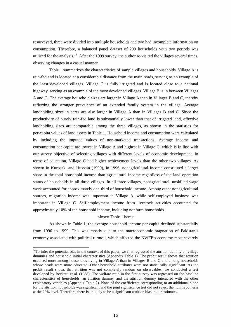
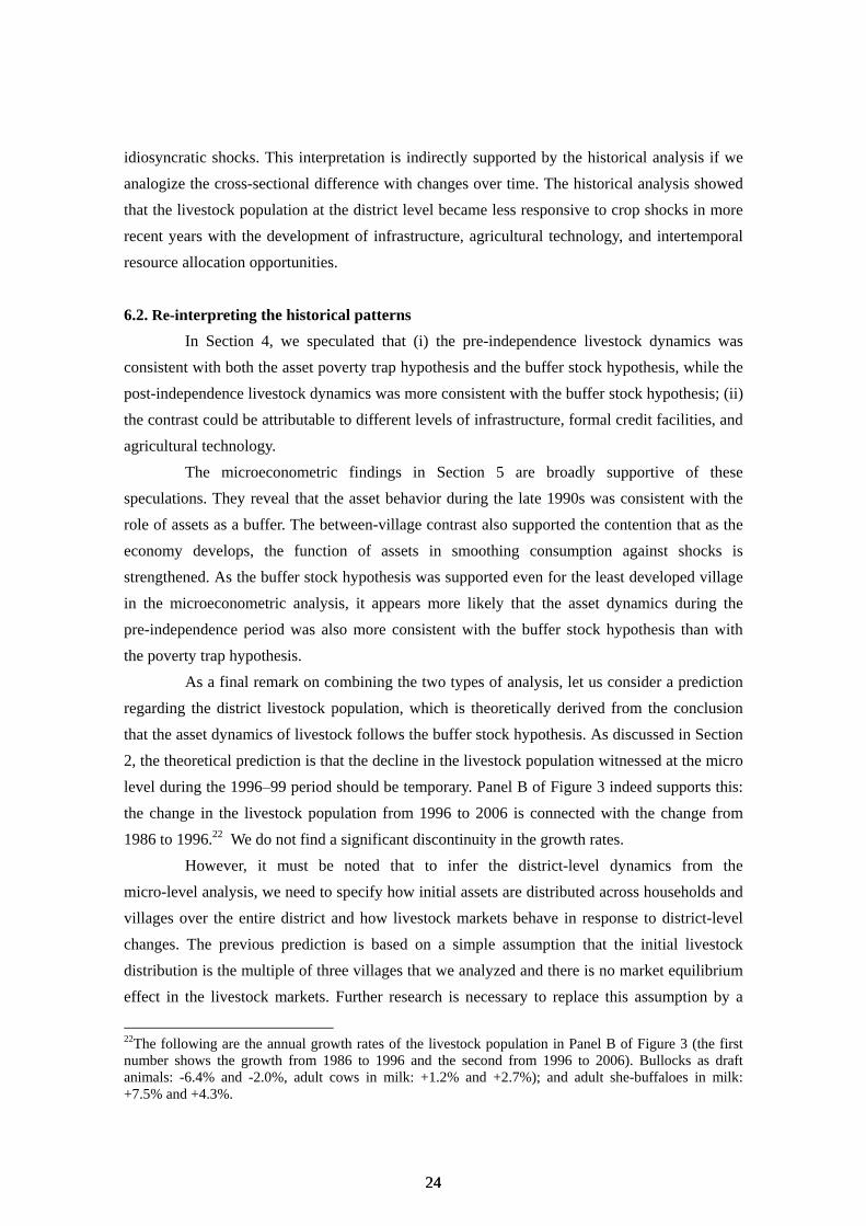

800
700
600
500
400
300
200
100
0
2250
2000
1750
1500
1250
1000
750
500
250
B Peshawar District
1903
1905
1907
1909
1911
1913
1915
1917
1931
1933
1935
1937
1939
1941
1943
1945
1903
1905
1907
1909
1911
1913
1915
1917
1931
1933
1935
1937
1939
1941
1943
1945
Figure 2 Crop Production and Livestock in the NWFP before Partition (1903ndash1945)
A The NWFP
wheat_a kharif_a rabi_a fail_a bull cow buf_f
Note (1) Crop variables (wheat_a kharif_a rabi_a and fail_a) are plotted on the left axis (unit 1000 acres) (2) Livestock numbers (bull cow and buf_f) are plotted on the right axis (unit 1000 heads) (3) Peshawar District corresponds to the district borders until 1937 It comprises the current districts of Peshawar Charsadda Nowshera Mardan and Swabi
Source Created by the author using the dataset described in the text (the same for the following figures)
1919
19
19
1921
19
21
1923
19
23
1925
19
25
1927
19
27
1929
19
29
160
140
120
100
80
60
40
20
0
450
400
350
300
250
200
150
100
50
3030
Figure 3 Crop Production in the NWFP after Partition (1948ndash2011) A The NWFP
0
200
400
600
800
1000
1200
1400
1600
1800
2000
0
50
100
150
200
250
300
B Peshawar District
0
50
100
150
200
250
0
50
100
150
200
250
300
wheat_a wheat_y maize_a maize_y
bull cow buf_f
Note (1) Crop variables (wheat_a wheat_y maize_a and maize_y) are plotted on the left axis (unitindex with 1948 = 100 The absolute level in 1948 for the four variables are 410 (1000 ha) 695(kgha) 190 (1000 ha) 995 (kgha) for the NWFP and 68 (1000 ha) 828 (kgha) 36 (1000 ha) 1550(kgha) for Peshawar (2) Livestock numbers (bull cow and buf_f) are plotted on the right axis (unit1000 heads) (3) Peshawar District corresponds to the district borders in 1948 It comprises the current districts of Peshawar Charsadda and Nowshera
1948
1950
1952
1954
1956
1958
1960
1962
1964
1966
1968
1948
1950
1952
1954
1956
1958
1960
1962
1964
1966
1968
1970
19
70
1972
19
72
1974
19
74
1976
19
76
3131
1978
19
78
1980
19
80
1982
19
82
1984
19
84
1986
19
86
1988
1990
1992
1994
1996
1998
2000
2002
2004
2006
2008
2010
1988
1990
1992
1994
1996
1998
2000
2002
2004
2006
2008
2010
Figure 4Nonparametrically Estimated Asset Dynamics Curves Pakistan (NWFP) 1996ndash1999
A Livestock per capita (unit Rs 1000 at 1996 prices)
B Owned farmland per capita (unit Rs 100000 at 1996 prices)
3232
C The livelihood asset (unit the poverty line)
Notes Nonparametrically estimated by LOWESS with a bandwidth of 08 The scatter plots on the vertical axis are raw observations without any control
3333
Figure 5Parametrically Estimated Asset Dynamics Curves Pakistan (the NWFP) 1996ndash1999
A Livestock per capita (unit Rs 1000 at 1996 prices)
B Owned farmland per capita (unit Rs 100000 at 1996 prices)
3434
C The livelihood asset (unit the poverty line)
Notes Parametrically estimated by OLS The scatter plots on the vertical axis are raw observations net of
asset changes predicted by other controls included in Table 2
3535
Table 1 Characteristics of the Sample Households in the 1996ndash99 Panel Survey the NWFP Pakistan
Variable Village A Village B Village C
1 Village characteristics
Agriculture Rain-fed Rainirrig Irrigated
Distance to main roads (km) 10 4 1
Population (1998 Census) 2858 3831 7575
Adult literacy rates in (1998 Census) 258 199 375
2 Characteristics of households in the panel
Number of households 83 111 105
Average of initial characteristics in the 1996 survey1
Household size 1075 841 895
Literacy rate of working-age adults () 168 176 313
Average farmland owned (acres) 551 128 143
Per-capita value2 of farmland asset (Rs 1000003)
in the 1996 survey 0475 0804 0376
in the 1999 survey 0306 0417 0394
Per-capita value2 of livestock asset (Rs 10003)
in the 1996 survey 1525 1181 1884
in the 1999 survey 1087 0727 1042
Per-capita income2 (poverty line units4)
in the 1996 survey 1074 1278 1861
in the 1999 survey 0856 0953 1225
Per-capita consumption2 (poverty line units4)
in the 1996 survey 0743 0868 1110
in the 1999 survey 0773 0828 1148
Notes (1) ldquoAverage of initial characteristicsrdquo represents the average over all sample households (2) ldquoPer-capita valuerdquo represents the average based on individuals It is calculated with the number of household members as weights (3) ldquoRsrdquo indicates Pakistani Rupees in 1996 prices adjusted for inflation (4) The same poverty line (but different for 1996 and 1999 adjusted for inflation) was used for both income and consumption and for all villages to convert per-capita income (consumption) into poverty line units Source Prepared by the author using the 1996ndash99 panel data described in the text (same for the following tables)
3636
Table 2 Response of Assets to Village- and Household-level Shocks
Dependent variable Change in assets from 1996 to 1999
D_livestock D_farmland D_livelihood asset
Initial level of each asset
Linear -0801 -0340 -0421
[0210] [0085] [0186]
Squared -0023 0300 0233
[0085] [0203] [0637]
Cubic 0049 -0155 1179
[0053] [0072] [0749]
Fourth degree -0007 0021 -1325
[0006] [0009] [1062]
Fifth degree 0000 -0001 0269
[0000] [0000] [0803]
Demographic controls
Initial hh size -0019 0012 0007
[0015] [0008] [0007]
D_hh size -0031 -0021 -0023
[0017] [0012] [0005]
Literacy rate of working-age adults -0329 0429 0106
[0360] [0131] [0136]
Response to village-level shock (coefficient on the fixed effect)
Village A -0656 -0272 0020
[0137] [0088] [0050]
Village B -0699 -0109 -0009
[0178] [0083] [0054]
Village C -0446 -0097 0100
[0164] [0078] [0029]
Response to household-level shock
Agricultural shock -0003 -0021 -0033
[0122] [0080] [0032]
Off-farm work shock -0072 0065 -0055
[0233] [0088] [0046]
Other shocks -0200 -0138 -0047
[0151] [0061] [0040]
R-squared 0784 0389 0314
F-stat for zero coef on non-linear terms 750 297 373
F-stat for homogenous village fe 087 335 185
F-stat for zero coef on hh-level shocks 065 206 148
3737
Notes to Table 2 (1) Huber-White robust standard errors are given in square brackets (2) and represent statistical significance at the 1 5 and 10 levels respectively (3) WLS regression with village fixed effects (no intercept) is employed where weights are the number of household members inflated by village-specific inflation factors (4) To make the coefficients on village fixed effects readily interpretable the initial asset hh size and literacy rates are replaced by their deviations from the mean See Table 1 and Appendix Table 3 for the summary statistics of these variables (5) The following are the definitions and statistics of household-level shocks
ldquoAgricultural shockrdquo = Index of agricultural shocks that the household experienced between 1996 and 1999 If the household experienced both crop failure and output prices lower than the market rate +2 if it experienced either +1 if it experienced neither 0 if it experienced either of bumper crop harvest or output prices higher than the market rate -1 if it experienced both -2 The mean is -0074 and the standard deviation is 0721
ldquoOff-farm work shockrdquo = Index of shocks to the off-farm work conditions of the household between 1996 and 1999 If the household experienced both the loss of employment and a decrease in wage rates +2 if it experienced either +1 if it experienced neither 0 if it experienced either of the gain in employment or the increase in wage rates -1 if it experienced both -2 The mean is 0036 and the standard deviation is 0532
ldquoOther shockrdquo = Index of other shocks that the household experienced between 1996 and 1999 such as unexpected deaths and funerals and discontinuation of remittances from family members living outside the village If it is a negative shock +1 if there was no such shock 0 if it is a positive shock -1 The mean is 0098 and the standard deviation is 0565
3838
Appendix Table 1 Correlates of Attrition (Probit Regression Result)
Dependent variable retention (dummy variable for being included in the panel data analysis)
Coef [SE] dPdX
Village-specific intercept Village A 0749 [0260] 0156 Village B 1945 [0307] 0406 Village C 1404 [0262] 0293
Households initial characteristics Household size -0075 [0142] -0016 Ratio of dependent members 0047 [0084] 0010 Age of household head -0014 [0102] -0003 Dummy for nonfarm fulltime employees -0045 [0189] -0009 Dummy for regular remittance receipt -0387 [0337] -0081 Land ownership dummy -0114 [0205] -0024 Land asset value 0319 [0506] 0066 Livestock value 0197 [0207] 0041 Net monetary asset -0022 [0125] -0005 Other asset value 0388 [0389] 0081 Education of household head -0201 [0091] -0042
Log likelihood -1334 Fraction of correct prediction 0848 LR test (chi2) for zero slopes of all explanatory variables 4270 LR test (chi2) for zero slopes of households initial characteristics 1226
Notes (1) Standard errors [SE] were robust standard errors computed from analytical second derivatives Continuous variables in Households initial characteristics are normalized by their means and standard errors (2) Statistically significant at the 1 () 5 () and 10 () level (3) The number of observations is 355
3939
Appendix Table 2 Welfare Level and the Attrition Status
Dependent variable Welfare ratio
Additional slope for theBase slope
attritor households
Village-specific intercept Village A 1040 [0142] -0214 [0239] Village B 1140 [0138] -0309 [0306] Village C 1248 [0147] -0436 [0237]
Household wealth characteristics Household size -0012 [0007] -0006 [0010] Ratio of females -0042 [0165] 0190 [0372] Ratio of dependent members -0532 [0154] 0370 [0301] Dummy for a female-headed household -0275 [0132] (dropped) Age of the household head -0001 [0002] 0004 [0003] Literacy rate of working-age adults 0311 [0119] 0024 [0193] Per-capita value of assets other than those below 0014 [0007] 0027 [0027] Per-capita outstanding credit 0017 [0003] 0030 [0019] Per-capita value of farmland 0081 [0020] -0100 [0080] Per-capita value of livestock 0041 [0013] -0031 [0018] Dummy for non-agricultural employment permanent 0010 [0054] -0120 [0098] Dummy for regular remittance receipt 0183 [0110] -0255 [0185]
R-squared 0896 F-stat for zero coef on all base slopes and the same coeff of village-spec intercept 1255 F-stat for zero coef on all additional slopes interacted with the attrition dummy 124
Notes See Appendix Table 3 for summary statistics of the explanatory variables The additional slope for the attritor households wrt female headed household was dropped as no such household dropped out of the sample
4040
Appendix Table 3 Estimation of the Livelihood Asset through Regression Analysis
Dependent variable Welfare ratio 1996 1999
Summary Regression Summary Regression statistics results statistics results
Village-specific intercept Village A 0201 1003 0206 0937
(0402) [0115] (0405) [0131] Village B 0270 1104 0251 0948
(0444) [0117] (0434) [0120] Village C 0529 1197 0544 1123
(0500) [0123] (0499) [0121] Household wealth characteristics
Number of household members 11843 -0012 12222 -0006 (6854) [0006] (7606) [0005]
Ratio of females in the household 0484 -0017 0483 0070 (0129) [0143] (0126) [0182]
Ratio of dependent members in the household 0488 -0481 0492 -0644 (0184) [0136] (0189) [0133]
Dummy for a female-headed household 0005 -0261 0014 0007 (0072) [0121] (0118) [0128]
Age of the household head 52259 -0001 54735 0001 (16411) [0001] (15809) [0001]
Literacy rate of working-age adults 0278 0349 0323 0176 (0257) [0101] (0258) [0092]
Per-capita value of household assets such as 2494 0015 0597 0219 agricultural machinery transport equipment (6259) [0007] (0963) [0043] durable goods etc (Rs 1000 in 1996 prices) Per-capita outstanding credit including informal 0967 0017 0719 0013 lending to others (Rs 1000 in 1996 prices) (5778) [0003] (3605) [0013] Per-capita value of farmland owned by the 0488 0081 0366 0120 household (Rs 100000 in 1996 prices) (1500) [0020] (0919) [0024] Per-capita value of livestock owned by the 1531 0039 0934 0060 household (Rs 100000 in 1996 prices) (2656) [0011] (1297) [0034] Dummy for a household with workers employed in 0551 -0013 0583 -0089 nonagricultural employment on a permanent basis (0498) [0047] (0494) [0043] Dummy for a household that regularly receives 0086 0164 0184 0127 remittances from family members living separately (0281) [0097] (0388) [0075]
Mean of the depvar R-squared 0957 0893 0994 0902 (StdDev) of the depvar F-stat for zero slopes (0473) 1428 (0512) 1571 Number of observations 354 354 351 351
Notes (1) In the summary statistics column weighted means are reported with standard deviations shown in parentheses (2) Huber-White robust standard errors are shown in brackets (3) WLS regression with village fixed effects (no intercept) is employed (4) Weights are the same as those described in Table 2 (5) Statistically significant at the 1 () 5 () and 10 () level (6) In the 1996 regression the number of observations is 344 as one observation was excluded due to the non-availability of consumption data In the 1999 regression the number of observation is 351 as we included split and replacement households
4141
Appendix Table 4 Test for Convergence
Dependent variable Change in assets from 1996 to 1999
D_livestock D_farmland D_livelihood asset
Evaluated at the 25 percentile Point estimate of the slope on the lagged asset -0265 -0788 -0289
F-statistics for the null that the slope is zero 023 667 120
p-value 06329 00103 02749
F-statistics for the null that the slope is -2 1010 1580 4232
p-value 00016 00001 00000
Evaluated at the median Point estimate of the slope on the lagged asset -0661 -0737 -0434
F-statistics for the null that the slope is zero 3245 705 664
p-value 00000 00084 00105
F-statistics for the null that the slope is -2 13287 2072 8670
p-value 00000 00000 00000
Evaluated at the 75 percentile Point estimate of the slope on the lagged asset -0792 -0383 -0293
F-statistics for the null that the slope is zero 1052 1543 115
p-value 00013 00001 02847
F-statistics for the null that the slope is -2 2445 27509 3905
p-value 00000 00000 00000
Notes Point estimates and test statistics are based on specifications reported in Table 2 If the null hypothesis is rejected in favor of the point estimate between -2 and 0 local convergence evaluated at each percentile is suggested
4242
Appendix Table 5 Robustness Check 1 (Addition of More Controls)
Dependent variable Change in assets from 1996 to 1999
D_livestock D_farmland D_livelihood asset
Initial level of each asset Linear -0797 -0324 -0260
[0214] [0087] [0436] Squared -0013 0338 0964
[0085] [0211] [0722] Cubic 0046 -0169 0937
[0054] [0076] [0727] 4th degree -0007 0023 -2606
[0006] [0009] [1253] 5th degree 0000 -0001 1057
[0000] [0000] [0907] Demographic controls
Initial hh size -0020 0015 0013 [0017] [0011] [0008]
D_hh size -0028 -0022 -0025 [0018] [0013] [0005]
Literacy rate of working-age adults -0275 0442 0067 [0364] [0134] [0192]
Other initial household assets
Ratio of females in the household 0763 0149 -0023 [0576] [0176] [0136]
Ratio of dependent members in the -0133 -0257 -0113 household [0601] [0210] [0228] Age of the household head 0005 -0001 -0002
[0005] [0003] [0002] Per-capita value of other hh assets -0004 -0003 -0012
[0012] [0007] [0010] Per-capita outstanding credit -0002 -0006 -0008
[0020] [0006] [0008] Response to village-level shock (coefficient on the fixed effect)
Village A -0665 -0297 -0029 [0146] [0095] [0055]
Village B -0714 -0113 -0052 [0185] [0082] [0046]
Village C -0461 -0099 0076 [0167] [0078] [0032]
Response to household-level shock Agricultural shock -0017 -0023 -0027
[0121] [0080] [0028] Off farm work shock -0039 0058 -0063
[0250] [0083] [0046] Other shock -0204 -0134 -0045
[0155] [0062] [0038] R-squared 0786 0396 0360 F-stat for zero coef on non-linear terms 696 311 598 F-stat for homogenous village fe 076 367 358 F-stat for zero coef on hh-level shocks 071 184 164
Notes See Table 2 Summary statistics of the additional variables under Other initial household assets are provided in Appendix Table 3 From the list of potential controls in Appendix Table 3 continuous variables were added to the regression because the addition of dummy variables resulted in a high level of multicollinearity in our dataset
4343
Reference Table 6 Robustness Check 2 (Unweighted Regression Results)
Dependent variable Change in assets from 1996 to 1999
D_livestock D_farmland D_livelihood asset
Initial level of each asset Linear -0762 -0414 -0376
[0179] [0081] [0149] Squared -0033 0134 0898
[0074] [0219] [0477] Cubic 0050 -0062 0781
[0046] [0095] [0592] Fourth degree -0007 0007 -2230
[0005] [0013] [0842] Fifth degree 0000 0000 0838
[0000] [0001] [0623] Demographic controls
Initial hh size -0016 0010 0000 [0018] [0009] [0005]
D_hh size -0033 -0025 -0026 [0017] [0011] [0004]
Literacy rate of working-age adults -0215 0328 0059 [0340] [0106] [0091]
Response to village-level shock (coefficient on the fixed effect) Village A -0594 -0169 -0006
[0117] [0072] [0043] Village B -0679 -0081 -0066
[0160] [0081] [0042] Village C -0387 -0051 0090
[0157] [0068] [0030] Response to household-level shock
Agricultural shock 0043 -0062 0001 [0136] [0087] [0028]
Off farm work shock -0021 0057 -0048 [0200] [0074] [0038]
Other shock -0206 -0086 -0073 [0120] [0049] [0031]
R-squared 0631 0503 0283 F-stat for zero coef on non-linear terms 1211 107 480 F-stat for homogenous village fe 108 221 563 F-stat for zero coef on hh-level shocks 109 105 251
Notes Esimated by OLS See Table 2 for other notes
4444
Appendix Table 7 Robustness Check 3 (Disaggregated Household-level Shocks)
Dependent variable Change in assets from 1996 to 1999
D_livestock D_farmland D_livelihood asset
Initial level of each asset Linear -0749 -0432 -0370
[0179] [0077] [0151] Squared -0039 0169 0919
[0075] [0217] [0480] Cubic 0050 -0077 0754
[0046] [0094] [0601] Fourth degree -0007 0009 -2289
[0005] [0013] [0862] Fifth degree 0000 0000 0884
[0000] [0001] [0644] Demographic controls
Initial hh size -0012 0012 0001 [0017] [0010] [0005]
D_hh size -0030 -0024 -0026 [0017] [0011] [0004]
Literacy rate of working-age adults -0272 0288 0051 [0347] [0098] [0094]
Response to village-level shock (coefficient on the fixed effect) Village A -0598 -0187 -0007
[0117] [0071] [0043] Village B -0635 -0093 -0066
[0160] [0076] [0042] Village C -0357 -0064 0089
[0162] [0066] [0031] Response to household-level shock
Agricultural shock crop failure 0036 0084 0031 [0300] [0108] [0047]
Agricultural shock price fall 0038 -0232 -0035 [0260] [0125] [0046]
Off farm work shock loss of employme -0396 -0091 -0068 [0331] [0059] [0058]
Off farm work shock wage fall 0277 0156 -0037 [0216] [0137] [0043]
Other shock -0224 -0093 -0073 [0122] [0051] [0032]
R-squared 0636 0511 0286 F-stat for zero coef on non-linear terms 1271 120 493 F-stat for homogenous village fe 110 232 549 F-stat for zero coef on hh-level shocks 126 135 156
Notes Agricultural shock and Off farm work shock in Table 2 are disaggregated into 2 variables each Now the all of the five shock variables are indicators variable taking the values of -1 0 and 1 See Table 2 for other notes
4545
Appendix Table 8 Robustness Check 4 (Aggregated Household-level Shocks)
Dependent variable Change in assets from 1996 to 1999
D_livestock D_farmland D_livelihood asset
Initial level of each asset Linear -0744 -0419 -0361
[0180] [0082] [0151] Squared -0027 0142 0886
[0074] [0232] [0482] Cubic 0045 -0065 0751
[0046] [0099] [0592] Fourth degree -0007 0007 -2249
[0005] [0014] [0868] Fifth degree 0000 0000 0861
[0000] [0001] [0630] Demographic controls
Initial hh size -0018 0009 0000 [0018] [0009] [0005]
D_hh size -0035 -0027 -0026 [0017] [0012] [0005]
Literacy rate of working-age adults -0200 0346 0060 [0343] [0111] [0092]
Response to village-level shock (coefficient on the fixed effect) Village A -0604 -0166 -0006
[0118] [0072] [0042] Village B -0711 -0086 -0071
[0155] [0079] [0041] Village C -0416 -0058 0085
[0160] [0069] [0030] Response to household-level shock
Sum of the three types of shocks -0048 -0035 -0035 [0085] [0029] [0017]
R-squared 0629 0499 0276 F-stat for zero coef on non-linear terms 1231 112 443 F-stat for homogenous village fe 112 198 548
Notes Agricultural shock Off farm work shock and Other shock in Table 2 are added to construct one householdlevel shock variable It is an indicator variable taking the values of -3 -2 -1 0 1 2 and 3 See Table 2 for other notes
46
Appendix Table 9 Robustness Check 5 (Change in Household Size Excluded)
Dependent variable Change in assets from 1996 to 1999
D_livestock D_farmland D_livelihood asset
Initial level of each asset Linear -0846 -0398 -0542
[0210] [0090] [0199] Squared -0012 0369 -0005
[0086] [0223] [0645] Cubic 0052 -0176 1067
[0054] [0078] [0820] Fourth degree -0008 0024 0161
[0006] [0009] [1075] Fifth degree 0000 -0001 -0594
[0000] [0000] [0859] Demographic controls
Initial hh size -0005 0020 0012 [0014] [0010] [0006]
Literacy rate of working-age adults -0390 0390 0126 [0369] [0133] [0151]
Response to village-level shock (coefficient on the fixed effect) Village A -0665 -0283 -0012
[0133] [0086] [0053] Village B -0680 -0110 0013
[0183] [0084] [0058] Village C -0461 -0114 0121
[0165] [0083] [0031] Response to household-level shock
Agricultural shock 0003 -0012 -0029 [0125] [0080] [0034]
Off farm work shock -0028 0095 -0021 [0243] [0095] [0047]
Other shock -0279 -0189 -0106 [0139] [0080] [0045]
R-squared 0781 0371 0226 F-stat for zero coef on non-linear terms 678 283 078 F-stat for homogenous village fe 067 395 298 F-stat for zero coef on hh-level shocks 164 217 234
Notes D_hh size in Table 2 is excluded from the regression as the variable is more endogenous than others See Table 2 for other notes
47
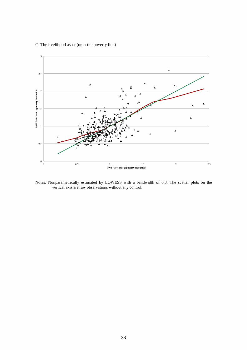
C The livelihood asset (unit the poverty line)
Notes Nonparametrically estimated by LOWESS with a bandwidth of 08 The scatter plots on the vertical axis are raw observations without any control
3333
Figure 5Parametrically Estimated Asset Dynamics Curves Pakistan (the NWFP) 1996ndash1999
A Livestock per capita (unit Rs 1000 at 1996 prices)
B Owned farmland per capita (unit Rs 100000 at 1996 prices)
3434
C The livelihood asset (unit the poverty line)
Notes Parametrically estimated by OLS The scatter plots on the vertical axis are raw observations net of
asset changes predicted by other controls included in Table 2
3535
Table 1 Characteristics of the Sample Households in the 1996ndash99 Panel Survey the NWFP Pakistan
Variable Village A Village B Village C
1 Village characteristics
Agriculture Rain-fed Rainirrig Irrigated
Distance to main roads (km) 10 4 1
Population (1998 Census) 2858 3831 7575
Adult literacy rates in (1998 Census) 258 199 375
2 Characteristics of households in the panel
Number of households 83 111 105
Average of initial characteristics in the 1996 survey1
Household size 1075 841 895
Literacy rate of working-age adults () 168 176 313
Average farmland owned (acres) 551 128 143
Per-capita value2 of farmland asset (Rs 1000003)
in the 1996 survey 0475 0804 0376
in the 1999 survey 0306 0417 0394
Per-capita value2 of livestock asset (Rs 10003)
in the 1996 survey 1525 1181 1884
in the 1999 survey 1087 0727 1042
Per-capita income2 (poverty line units4)
in the 1996 survey 1074 1278 1861
in the 1999 survey 0856 0953 1225
Per-capita consumption2 (poverty line units4)
in the 1996 survey 0743 0868 1110
in the 1999 survey 0773 0828 1148
Notes (1) ldquoAverage of initial characteristicsrdquo represents the average over all sample households (2) ldquoPer-capita valuerdquo represents the average based on individuals It is calculated with the number of household members as weights (3) ldquoRsrdquo indicates Pakistani Rupees in 1996 prices adjusted for inflation (4) The same poverty line (but different for 1996 and 1999 adjusted for inflation) was used for both income and consumption and for all villages to convert per-capita income (consumption) into poverty line units Source Prepared by the author using the 1996ndash99 panel data described in the text (same for the following tables)
3636
Table 2 Response of Assets to Village- and Household-level Shocks
Dependent variable Change in assets from 1996 to 1999
D_livestock D_farmland D_livelihood asset
Initial level of each asset
Linear -0801 -0340 -0421
[0210] [0085] [0186]
Squared -0023 0300 0233
[0085] [0203] [0637]
Cubic 0049 -0155 1179
[0053] [0072] [0749]
Fourth degree -0007 0021 -1325
[0006] [0009] [1062]
Fifth degree 0000 -0001 0269
[0000] [0000] [0803]
Demographic controls
Initial hh size -0019 0012 0007
[0015] [0008] [0007]
D_hh size -0031 -0021 -0023
[0017] [0012] [0005]
Literacy rate of working-age adults -0329 0429 0106
[0360] [0131] [0136]
Response to village-level shock (coefficient on the fixed effect)
Village A -0656 -0272 0020
[0137] [0088] [0050]
Village B -0699 -0109 -0009
[0178] [0083] [0054]
Village C -0446 -0097 0100
[0164] [0078] [0029]
Response to household-level shock
Agricultural shock -0003 -0021 -0033
[0122] [0080] [0032]
Off-farm work shock -0072 0065 -0055
[0233] [0088] [0046]
Other shocks -0200 -0138 -0047
[0151] [0061] [0040]
R-squared 0784 0389 0314
F-stat for zero coef on non-linear terms 750 297 373
F-stat for homogenous village fe 087 335 185
F-stat for zero coef on hh-level shocks 065 206 148
3737
Notes to Table 2 (1) Huber-White robust standard errors are given in square brackets (2) and represent statistical significance at the 1 5 and 10 levels respectively (3) WLS regression with village fixed effects (no intercept) is employed where weights are the number of household members inflated by village-specific inflation factors (4) To make the coefficients on village fixed effects readily interpretable the initial asset hh size and literacy rates are replaced by their deviations from the mean See Table 1 and Appendix Table 3 for the summary statistics of these variables (5) The following are the definitions and statistics of household-level shocks
ldquoAgricultural shockrdquo = Index of agricultural shocks that the household experienced between 1996 and 1999 If the household experienced both crop failure and output prices lower than the market rate +2 if it experienced either +1 if it experienced neither 0 if it experienced either of bumper crop harvest or output prices higher than the market rate -1 if it experienced both -2 The mean is -0074 and the standard deviation is 0721
ldquoOff-farm work shockrdquo = Index of shocks to the off-farm work conditions of the household between 1996 and 1999 If the household experienced both the loss of employment and a decrease in wage rates +2 if it experienced either +1 if it experienced neither 0 if it experienced either of the gain in employment or the increase in wage rates -1 if it experienced both -2 The mean is 0036 and the standard deviation is 0532
ldquoOther shockrdquo = Index of other shocks that the household experienced between 1996 and 1999 such as unexpected deaths and funerals and discontinuation of remittances from family members living outside the village If it is a negative shock +1 if there was no such shock 0 if it is a positive shock -1 The mean is 0098 and the standard deviation is 0565
3838
Appendix Table 1 Correlates of Attrition (Probit Regression Result)
Dependent variable retention (dummy variable for being included in the panel data analysis)
Coef [SE] dPdX
Village-specific intercept Village A 0749 [0260] 0156 Village B 1945 [0307] 0406 Village C 1404 [0262] 0293
Households initial characteristics Household size -0075 [0142] -0016 Ratio of dependent members 0047 [0084] 0010 Age of household head -0014 [0102] -0003 Dummy for nonfarm fulltime employees -0045 [0189] -0009 Dummy for regular remittance receipt -0387 [0337] -0081 Land ownership dummy -0114 [0205] -0024 Land asset value 0319 [0506] 0066 Livestock value 0197 [0207] 0041 Net monetary asset -0022 [0125] -0005 Other asset value 0388 [0389] 0081 Education of household head -0201 [0091] -0042
Log likelihood -1334 Fraction of correct prediction 0848 LR test (chi2) for zero slopes of all explanatory variables 4270 LR test (chi2) for zero slopes of households initial characteristics 1226
Notes (1) Standard errors [SE] were robust standard errors computed from analytical second derivatives Continuous variables in Households initial characteristics are normalized by their means and standard errors (2) Statistically significant at the 1 () 5 () and 10 () level (3) The number of observations is 355
3939
Appendix Table 2 Welfare Level and the Attrition Status
Dependent variable Welfare ratio
Additional slope for theBase slope
attritor households
Village-specific intercept Village A 1040 [0142] -0214 [0239] Village B 1140 [0138] -0309 [0306] Village C 1248 [0147] -0436 [0237]
Household wealth characteristics Household size -0012 [0007] -0006 [0010] Ratio of females -0042 [0165] 0190 [0372] Ratio of dependent members -0532 [0154] 0370 [0301] Dummy for a female-headed household -0275 [0132] (dropped) Age of the household head -0001 [0002] 0004 [0003] Literacy rate of working-age adults 0311 [0119] 0024 [0193] Per-capita value of assets other than those below 0014 [0007] 0027 [0027] Per-capita outstanding credit 0017 [0003] 0030 [0019] Per-capita value of farmland 0081 [0020] -0100 [0080] Per-capita value of livestock 0041 [0013] -0031 [0018] Dummy for non-agricultural employment permanent 0010 [0054] -0120 [0098] Dummy for regular remittance receipt 0183 [0110] -0255 [0185]
R-squared 0896 F-stat for zero coef on all base slopes and the same coeff of village-spec intercept 1255 F-stat for zero coef on all additional slopes interacted with the attrition dummy 124
Notes See Appendix Table 3 for summary statistics of the explanatory variables The additional slope for the attritor households wrt female headed household was dropped as no such household dropped out of the sample
4040
Appendix Table 3 Estimation of the Livelihood Asset through Regression Analysis
Dependent variable Welfare ratio 1996 1999
Summary Regression Summary Regression statistics results statistics results
Village-specific intercept Village A 0201 1003 0206 0937
(0402) [0115] (0405) [0131] Village B 0270 1104 0251 0948
(0444) [0117] (0434) [0120] Village C 0529 1197 0544 1123
(0500) [0123] (0499) [0121] Household wealth characteristics
Number of household members 11843 -0012 12222 -0006 (6854) [0006] (7606) [0005]
Ratio of females in the household 0484 -0017 0483 0070 (0129) [0143] (0126) [0182]
Ratio of dependent members in the household 0488 -0481 0492 -0644 (0184) [0136] (0189) [0133]
Dummy for a female-headed household 0005 -0261 0014 0007 (0072) [0121] (0118) [0128]
Age of the household head 52259 -0001 54735 0001 (16411) [0001] (15809) [0001]
Literacy rate of working-age adults 0278 0349 0323 0176 (0257) [0101] (0258) [0092]
Per-capita value of household assets such as 2494 0015 0597 0219 agricultural machinery transport equipment (6259) [0007] (0963) [0043] durable goods etc (Rs 1000 in 1996 prices) Per-capita outstanding credit including informal 0967 0017 0719 0013 lending to others (Rs 1000 in 1996 prices) (5778) [0003] (3605) [0013] Per-capita value of farmland owned by the 0488 0081 0366 0120 household (Rs 100000 in 1996 prices) (1500) [0020] (0919) [0024] Per-capita value of livestock owned by the 1531 0039 0934 0060 household (Rs 100000 in 1996 prices) (2656) [0011] (1297) [0034] Dummy for a household with workers employed in 0551 -0013 0583 -0089 nonagricultural employment on a permanent basis (0498) [0047] (0494) [0043] Dummy for a household that regularly receives 0086 0164 0184 0127 remittances from family members living separately (0281) [0097] (0388) [0075]
Mean of the depvar R-squared 0957 0893 0994 0902 (StdDev) of the depvar F-stat for zero slopes (0473) 1428 (0512) 1571 Number of observations 354 354 351 351
Notes (1) In the summary statistics column weighted means are reported with standard deviations shown in parentheses (2) Huber-White robust standard errors are shown in brackets (3) WLS regression with village fixed effects (no intercept) is employed (4) Weights are the same as those described in Table 2 (5) Statistically significant at the 1 () 5 () and 10 () level (6) In the 1996 regression the number of observations is 344 as one observation was excluded due to the non-availability of consumption data In the 1999 regression the number of observation is 351 as we included split and replacement households
4141
Appendix Table 4 Test for Convergence
Dependent variable Change in assets from 1996 to 1999
D_livestock D_farmland D_livelihood asset
Evaluated at the 25 percentile Point estimate of the slope on the lagged asset -0265 -0788 -0289
F-statistics for the null that the slope is zero 023 667 120
p-value 06329 00103 02749
F-statistics for the null that the slope is -2 1010 1580 4232
p-value 00016 00001 00000
Evaluated at the median Point estimate of the slope on the lagged asset -0661 -0737 -0434
F-statistics for the null that the slope is zero 3245 705 664
p-value 00000 00084 00105
F-statistics for the null that the slope is -2 13287 2072 8670
p-value 00000 00000 00000
Evaluated at the 75 percentile Point estimate of the slope on the lagged asset -0792 -0383 -0293
F-statistics for the null that the slope is zero 1052 1543 115
p-value 00013 00001 02847
F-statistics for the null that the slope is -2 2445 27509 3905
p-value 00000 00000 00000
Notes Point estimates and test statistics are based on specifications reported in Table 2 If the null hypothesis is rejected in favor of the point estimate between -2 and 0 local convergence evaluated at each percentile is suggested
4242
Appendix Table 5 Robustness Check 1 (Addition of More Controls)
Dependent variable Change in assets from 1996 to 1999
D_livestock D_farmland D_livelihood asset
Initial level of each asset Linear -0797 -0324 -0260
[0214] [0087] [0436] Squared -0013 0338 0964
[0085] [0211] [0722] Cubic 0046 -0169 0937
[0054] [0076] [0727] 4th degree -0007 0023 -2606
[0006] [0009] [1253] 5th degree 0000 -0001 1057
[0000] [0000] [0907] Demographic controls
Initial hh size -0020 0015 0013 [0017] [0011] [0008]
D_hh size -0028 -0022 -0025 [0018] [0013] [0005]
Literacy rate of working-age adults -0275 0442 0067 [0364] [0134] [0192]
Other initial household assets
Ratio of females in the household 0763 0149 -0023 [0576] [0176] [0136]
Ratio of dependent members in the -0133 -0257 -0113 household [0601] [0210] [0228] Age of the household head 0005 -0001 -0002
[0005] [0003] [0002] Per-capita value of other hh assets -0004 -0003 -0012
[0012] [0007] [0010] Per-capita outstanding credit -0002 -0006 -0008
[0020] [0006] [0008] Response to village-level shock (coefficient on the fixed effect)
Village A -0665 -0297 -0029 [0146] [0095] [0055]
Village B -0714 -0113 -0052 [0185] [0082] [0046]
Village C -0461 -0099 0076 [0167] [0078] [0032]
Response to household-level shock Agricultural shock -0017 -0023 -0027
[0121] [0080] [0028] Off farm work shock -0039 0058 -0063
[0250] [0083] [0046] Other shock -0204 -0134 -0045
[0155] [0062] [0038] R-squared 0786 0396 0360 F-stat for zero coef on non-linear terms 696 311 598 F-stat for homogenous village fe 076 367 358 F-stat for zero coef on hh-level shocks 071 184 164
Notes See Table 2 Summary statistics of the additional variables under Other initial household assets are provided in Appendix Table 3 From the list of potential controls in Appendix Table 3 continuous variables were added to the regression because the addition of dummy variables resulted in a high level of multicollinearity in our dataset
4343
Reference Table 6 Robustness Check 2 (Unweighted Regression Results)
Dependent variable Change in assets from 1996 to 1999
D_livestock D_farmland D_livelihood asset
Initial level of each asset Linear -0762 -0414 -0376
[0179] [0081] [0149] Squared -0033 0134 0898
[0074] [0219] [0477] Cubic 0050 -0062 0781
[0046] [0095] [0592] Fourth degree -0007 0007 -2230
[0005] [0013] [0842] Fifth degree 0000 0000 0838
[0000] [0001] [0623] Demographic controls
Initial hh size -0016 0010 0000 [0018] [0009] [0005]
D_hh size -0033 -0025 -0026 [0017] [0011] [0004]
Literacy rate of working-age adults -0215 0328 0059 [0340] [0106] [0091]
Response to village-level shock (coefficient on the fixed effect) Village A -0594 -0169 -0006
[0117] [0072] [0043] Village B -0679 -0081 -0066
[0160] [0081] [0042] Village C -0387 -0051 0090
[0157] [0068] [0030] Response to household-level shock
Agricultural shock 0043 -0062 0001 [0136] [0087] [0028]
Off farm work shock -0021 0057 -0048 [0200] [0074] [0038]
Other shock -0206 -0086 -0073 [0120] [0049] [0031]
R-squared 0631 0503 0283 F-stat for zero coef on non-linear terms 1211 107 480 F-stat for homogenous village fe 108 221 563 F-stat for zero coef on hh-level shocks 109 105 251
Notes Esimated by OLS See Table 2 for other notes
4444
Appendix Table 7 Robustness Check 3 (Disaggregated Household-level Shocks)
Dependent variable Change in assets from 1996 to 1999
D_livestock D_farmland D_livelihood asset
Initial level of each asset Linear -0749 -0432 -0370
[0179] [0077] [0151] Squared -0039 0169 0919
[0075] [0217] [0480] Cubic 0050 -0077 0754
[0046] [0094] [0601] Fourth degree -0007 0009 -2289
[0005] [0013] [0862] Fifth degree 0000 0000 0884
[0000] [0001] [0644] Demographic controls
Initial hh size -0012 0012 0001 [0017] [0010] [0005]
D_hh size -0030 -0024 -0026 [0017] [0011] [0004]
Literacy rate of working-age adults -0272 0288 0051 [0347] [0098] [0094]
Response to village-level shock (coefficient on the fixed effect) Village A -0598 -0187 -0007
[0117] [0071] [0043] Village B -0635 -0093 -0066
[0160] [0076] [0042] Village C -0357 -0064 0089
[0162] [0066] [0031] Response to household-level shock
Agricultural shock crop failure 0036 0084 0031 [0300] [0108] [0047]
Agricultural shock price fall 0038 -0232 -0035 [0260] [0125] [0046]
Off farm work shock loss of employme -0396 -0091 -0068 [0331] [0059] [0058]
Off farm work shock wage fall 0277 0156 -0037 [0216] [0137] [0043]
Other shock -0224 -0093 -0073 [0122] [0051] [0032]
R-squared 0636 0511 0286 F-stat for zero coef on non-linear terms 1271 120 493 F-stat for homogenous village fe 110 232 549 F-stat for zero coef on hh-level shocks 126 135 156
Notes Agricultural shock and Off farm work shock in Table 2 are disaggregated into 2 variables each Now the all of the five shock variables are indicators variable taking the values of -1 0 and 1 See Table 2 for other notes
4545
Appendix Table 8 Robustness Check 4 (Aggregated Household-level Shocks)
Dependent variable Change in assets from 1996 to 1999
D_livestock D_farmland D_livelihood asset
Initial level of each asset Linear -0744 -0419 -0361
[0180] [0082] [0151] Squared -0027 0142 0886
[0074] [0232] [0482] Cubic 0045 -0065 0751
[0046] [0099] [0592] Fourth degree -0007 0007 -2249
[0005] [0014] [0868] Fifth degree 0000 0000 0861
[0000] [0001] [0630] Demographic controls
Initial hh size -0018 0009 0000 [0018] [0009] [0005]
D_hh size -0035 -0027 -0026 [0017] [0012] [0005]
Literacy rate of working-age adults -0200 0346 0060 [0343] [0111] [0092]
Response to village-level shock (coefficient on the fixed effect) Village A -0604 -0166 -0006
[0118] [0072] [0042] Village B -0711 -0086 -0071
[0155] [0079] [0041] Village C -0416 -0058 0085
[0160] [0069] [0030] Response to household-level shock
Sum of the three types of shocks -0048 -0035 -0035 [0085] [0029] [0017]
R-squared 0629 0499 0276 F-stat for zero coef on non-linear terms 1231 112 443 F-stat for homogenous village fe 112 198 548
Notes Agricultural shock Off farm work shock and Other shock in Table 2 are added to construct one householdlevel shock variable It is an indicator variable taking the values of -3 -2 -1 0 1 2 and 3 See Table 2 for other notes
46
Appendix Table 9 Robustness Check 5 (Change in Household Size Excluded)
Dependent variable Change in assets from 1996 to 1999
D_livestock D_farmland D_livelihood asset
Initial level of each asset Linear -0846 -0398 -0542
[0210] [0090] [0199] Squared -0012 0369 -0005
[0086] [0223] [0645] Cubic 0052 -0176 1067
[0054] [0078] [0820] Fourth degree -0008 0024 0161
[0006] [0009] [1075] Fifth degree 0000 -0001 -0594
[0000] [0000] [0859] Demographic controls
Initial hh size -0005 0020 0012 [0014] [0010] [0006]
Literacy rate of working-age adults -0390 0390 0126 [0369] [0133] [0151]
Response to village-level shock (coefficient on the fixed effect) Village A -0665 -0283 -0012
[0133] [0086] [0053] Village B -0680 -0110 0013
[0183] [0084] [0058] Village C -0461 -0114 0121
[0165] [0083] [0031] Response to household-level shock
Agricultural shock 0003 -0012 -0029 [0125] [0080] [0034]
Off farm work shock -0028 0095 -0021 [0243] [0095] [0047]
Other shock -0279 -0189 -0106 [0139] [0080] [0045]
R-squared 0781 0371 0226 F-stat for zero coef on non-linear terms 678 283 078 F-stat for homogenous village fe 067 395 298 F-stat for zero coef on hh-level shocks 164 217 234
Notes D_hh size in Table 2 is excluded from the regression as the variable is more endogenous than others See Table 2 for other notes
47
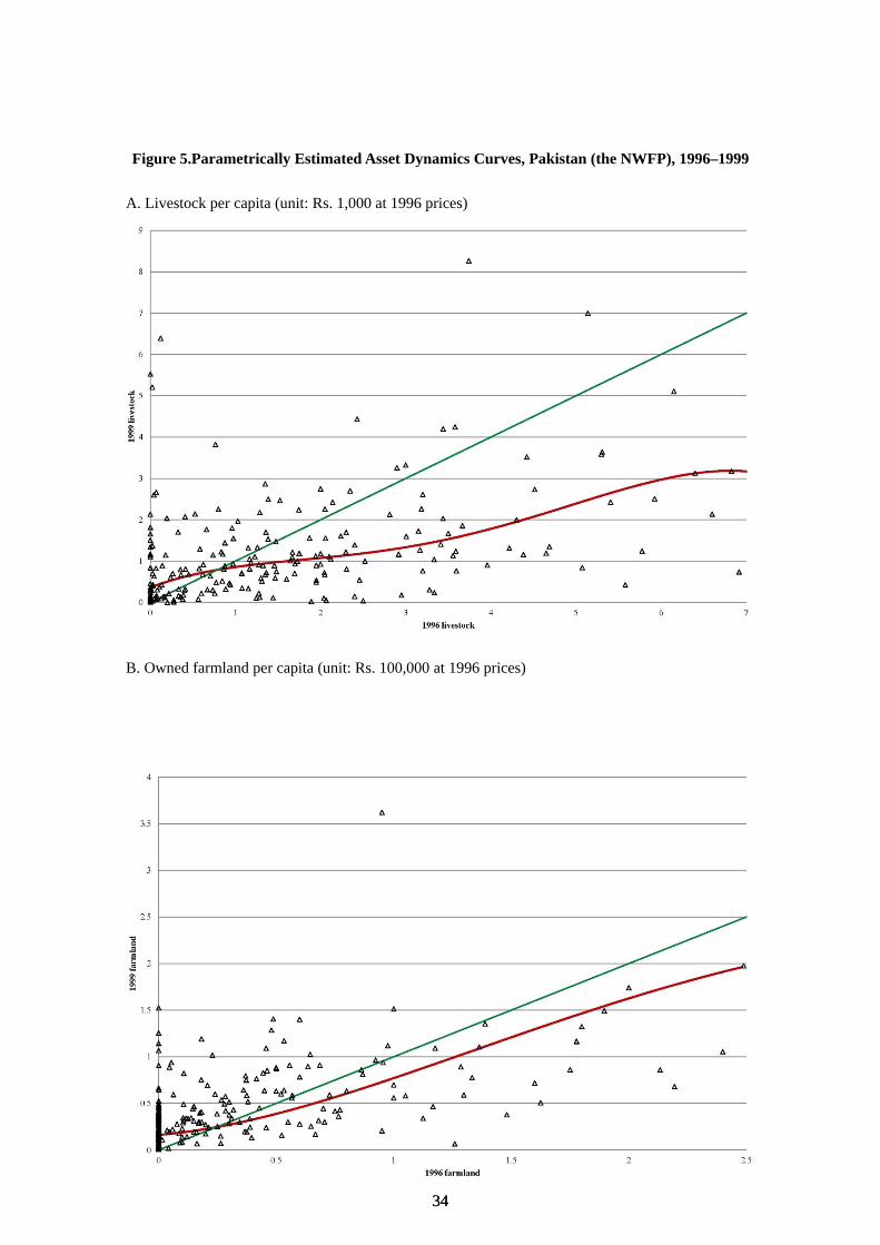
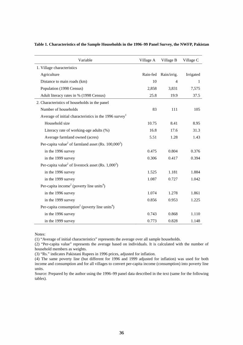
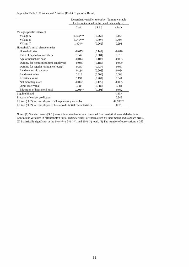
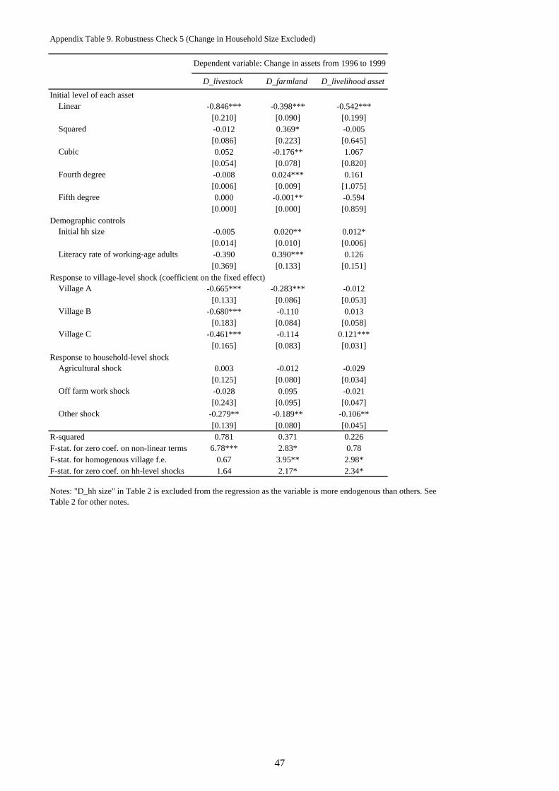