Dynamics of Feeder Cattle Basis and Price Slides

Kole Swanser Ph.D. Candidate

North Carolina State University

kswanse@ncsu.edu

Selected Paper prepared for presentation at the Agricultural & Applied

Economics Association’s 2013 AAEA & CAES Joint Annual Meeting,

Washington, DC, August 4-6, 2013.

Copyright 2013 by Kole Swanser. All rights reserved. Readers may make verbatim copies of this

document for non-commercial purposes by any means, provided this copyright notice appears on

all such copies.

Dynamics of Feeder Cattle Basis and Price Slides

Abstract

This study examines the dynamics of the relationship between per pound prices for feeder cattle

at different sale weights. The feeder cattle “price slide” relationship, as it is commonly known,

is influenced by fluctuations in the output price for slaughter cattle and the input price of feed

corn. I empirically test predictions about price slide dynamics that are derived from a two-input

derived demand model for slaughter cattle. Empirical analysis is conducted using an extensive

dataset of feeder cattle transactions.

1

I. Introduction

Changing cattle prices contribute to fluctuations in the value of beef cattle and represent

an important source of risk for all involved in the cattle industry. Futures markets can be useful

for managing this risk only to the extent that cattle basis – defined as the difference between the

per pound price for a standardized feeder cattle futures contract and the cash price for any

specific group (lot) of cattle – can be understood and predicted. Two of the most important

factors that influence feeder cattle prices and values are the price of finished cattle and the cost

of feed inputs. The former represents output price – it measures the value of fed cattle that have

reached a slaughter weight of around 1,250 pounds at the end of their production cycle. The

latter represents the most substantial variable cost component of producing finished cattle from

lighter feeder cattle.

Prices of standardized futures contracts for fed slaughter cattle and corn (a primary cattle

feeding input) are determined almost continuously on the Chicago Mercantile Exchange (CME).

In the same way that the value of a farmer’s standing crop depends on current futures price for

the commodity that can only be delivered after harvest, the value of a group of cattle today

depends on fed cattle prices in the future, when those animals are ready for slaughter. After

adjusting for time to slaughter, changes in fed cattle prices indicate changes in the expected

ending value of lighter weight cattle. The impact of corn prices on the value of unfinished cattle

is more complex. Changes in the cost of corn (a proxy for feed input cost) will have a disparate

effect on cattle according to weight. Since lighter animals require more feed to reach finishing

weight, the value of these animals is more sensitive to future feed costs. This has direct

implications for the risk associated with owning cattle. Specifically, lightweight cattle are more

exposed to value fluctuation resulting from corn price variability.

The fact that per pound prices for feeder cattle tend to decrease as sale weight increases is

well-known to market observers and has been studied and documented by agricultural

economists (Ehrich 1969, Buccola 1980, Marsh 1985, Dhuyvetter and Schroeder 2000). Within

the cattle industry, this price-weight relationship is commonly called the “price slide.” The slope

of the price slide is heavily influenced by the price of the feed inputs that will be used to add

weight to cattle. Constant changes in the shape of the cattle price slide reflect complex

interactions between dynamic markets for feed inputs and fed cattle and other feeder cattle price

2

determinants. Previous researchers have even documented extreme market conditions when per

pound prices for lightweight cattle have been discounted relative to heavier animals. These

unusual periods when the market exhibits an “inverted price slide” correspond to very high corn

prices relative to live cattle prices. Recent years have produced record high cattle and corn

prices and significant price fluctuations. We have also seen the rising importance of ethanol

production as a competing use for corn. These developments suggest that an updated analysis

using extensive current data may yield additional insights about these market dynamics.

My analysis of cattle and corn price dynamics begins by first developing predictions

about the relationship between futures price expectations and the cattle price slide using a two-

input slaughter cattle production model within a simple derived demand framework. I then

empirically test these predictions using a subset of data from a very large database of transaction-

level feeder cattle sales. This working paper concludes with a discussion about intended areas of

future research.

II. A Two-Input Derived Demand Model of Cattle Feeding

I generate predictions for the effects of cattle and corn prices on the slope of the price

slide using a simple two-input derived demand model.1 In this model, one finished steer for

slaughter is produced by combining one steer weighing 200 lbs. to 1,250 lbs. with the requisite

amount of a corn feed input.2 I make the simplifying assumption that cattle and corn are used in

fixed proportions, and that the quantity of corn input required can be calculated directly based on

the amount of weight gain required for the input steer to reach slaughter weight (assumed to be

exactly 1,250 lbs.).

The value of the output good, one finished steer, is determined by the market price of live

cattle. Factors that affect the market price of live cattle include the demand for live cattle, which

1 Two futures contracts for beef cattle are traded on the CME (Chicago Mercantile Exchange). The feeder cattle contract (FC) is for 650-850 pound steers. The live cattle futures contract (LC) is for live steers that are “finished” (fed to the appropriate weight) and ready to be slaughtered. Although the live cattle contract does not specify a weight range, finished steers typically weigh around 1,250 lbs. 2 A note on terminology is appropriate here. Curiously, there is no singular form of the word “cattle” in the English language that does not refer to a specific sex. Thus, I have chosen to use one feeder steer as the subject of my model illustration. Cattle that have not yet reached slaughter weight (approximately 1,250 lbs.) are typically called either feeder cattle (if 650 lbs. or heavier) or stocker cattle (if less than 650 lbs.). Feeder and stocker cattle are typically sold as either steers (castrated males) or heifers (females that have not yet given birth to a calf), although are bulls (males that have not been castrated) are commonly sold in some regions. The model presented here applies to heifers and bulls as well as steers.

3

is exogenous to the model, and the supply of live cattle. The beef production process is

characterized by long biological lags. This means that the current supply of live cattle for

slaughter is comprised of cattle that were born over 18 months earlier. Consequently, the future

supply of live cattle can be predicted well in advance of delivery based on current cattle

inventories. In this model I assume that cattle gain weight and progress through the beef

production and feeding process at a known constant rate. Thus, the supply of cattle in any given

weight group today will be equal to the supply of live cattle on the known future date when they

will all reach 1,250 lbs. This implies that current cash cattle prices for lighter weight animals are

linked to market conditions that are reflected in prices for heavier animals to be delivered in the

future.

Derived demand for the steer input in the two-input model can be obtained by subtracting

the cost of the corn feed input from the value of the finished 1,250 lb. steer output (following

Friedman 1962, chapter 7). The difference between the total value of the finished steer and the

total value of the input steer will be equal to the corn feed input cost. This difference is

commonly known as the gross feeding margin (GFM).

Example Feeder Cattle Model Calculations

An example using specific values for production coefficients, prices, and input variables

helps to illustrate the price slide relationship implied by the two-input derived demand model.

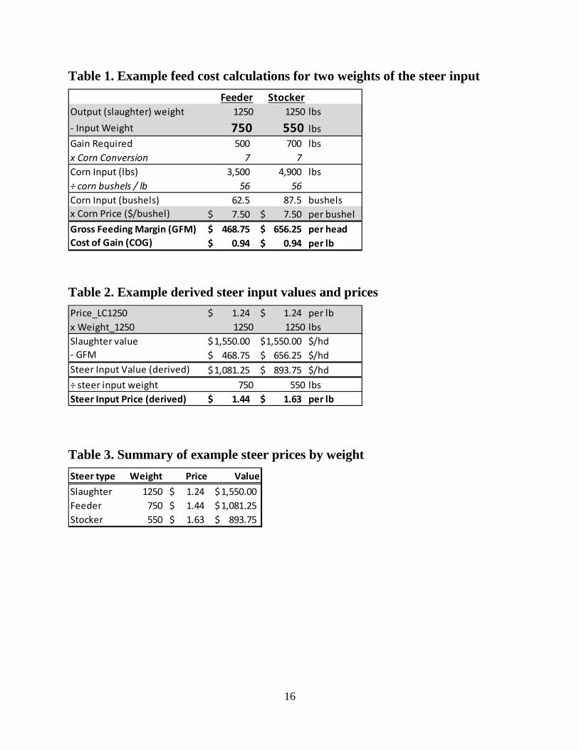
Table 1 displays feed requirement and cost calculations for two different weights of input steer: a

750 lb. “feeder” and a 550 lb. “stocker.” The calculations use a standard feed conversion factor

– seven pounds of corn grain are required to produce one pound of steer weight gain.3 Gray-

shaded values for input and output weights and corn prices (set initially at $7.50/bushel) are

considered to be exogenous. Since feed costs are linear with respect to weight, gross feeding

margin (GFM) is proportional to the weight of the input steer and per pound cost of gain (COG)

is equal for both steer types.

Derived values for the two weights of input steer are displayed in table 2. These are

calculated by subtracting the expected gross feeding margin calculated in table 1 from the

expected value of a finished 1,250 lb. steer. A live cattle futures price (LC1250) of $1.24 per

pound is used to calculate slaughter value for both weights of cattle in this example.

3 This conversion factor is common in the industry literature. See, for example, Anderson and Trapp 2000. Also note that one bushel of corn weighs 56 lbs.

4

Note that additional pounds of weight gain will always translate into greater value for

heavier steers in the two-input derived demand model as long as cost of gain is non-zero. At the

same time, we can see that the per pound price of a steer declines as sale weight increases. The

empirical analysis focuses on dynamics of the per pound price-weight relationship (the cattle

price slide).

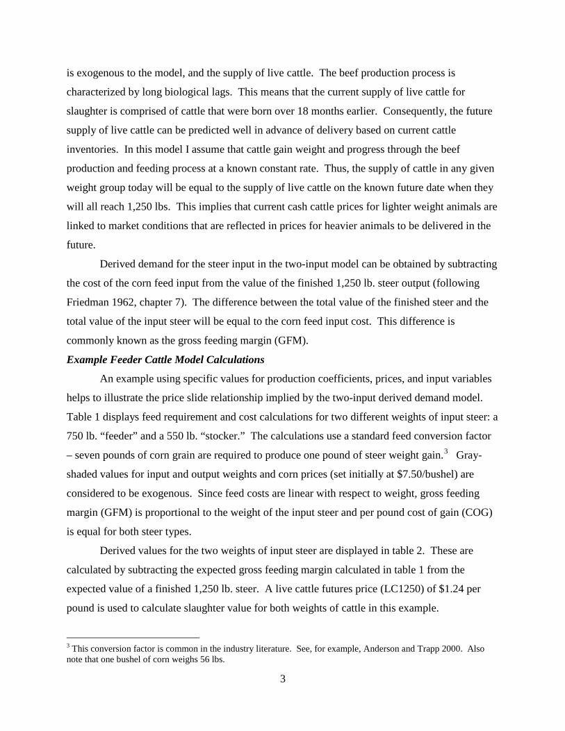
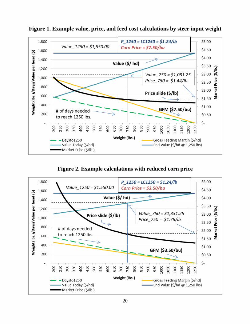
Figure 1 plots calculated values from the two-input derived demand model over a

spectrum of input steer weights ranging from 200 to 1,250 lbs. using example price and

production input values. The required gross feeding margin declines with input weight starting

from approximately $1,000 GFM for a 200 lb. steer input. Steer input value increases linearly at

the same rate until steer input weight equals slaughter weight, GFM is zero, and the steer input

value equals slaughter value (Value_1250). The implied per pound price for each weight of steer

input is also plotted on the right vertical axis. Note that the model parameters used in this

example produce a downward sloping price slide relationship with a convex curvature.

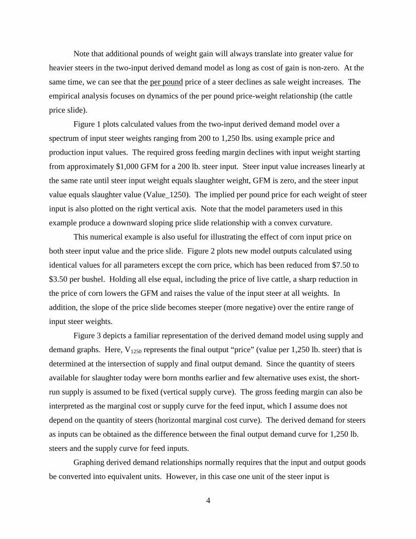
This numerical example is also useful for illustrating the effect of corn input price on

both steer input value and the price slide. Figure 2 plots new model outputs calculated using

identical values for all parameters except the corn price, which has been reduced from $7.50 to

$3.50 per bushel. Holding all else equal, including the price of live cattle, a sharp reduction in

the price of corn lowers the GFM and raises the value of the input steer at all weights. In

addition, the slope of the price slide becomes steeper (more negative) over the entire range of

input steer weights.

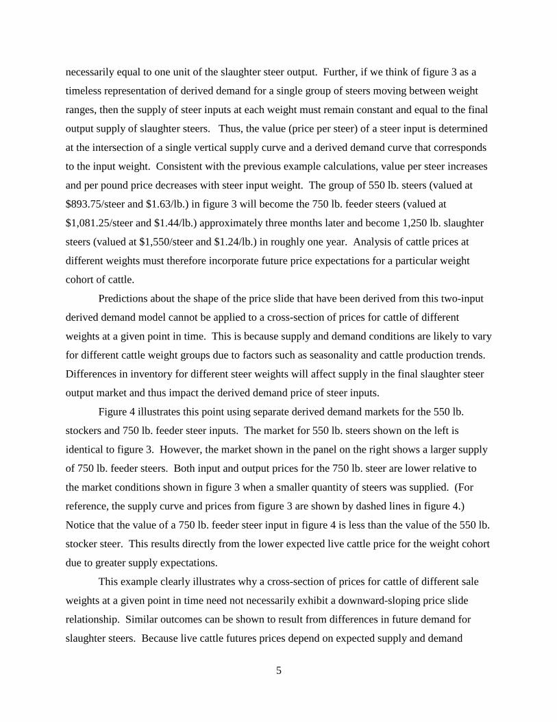
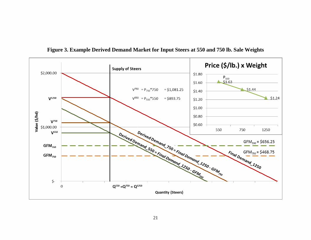
Figure 3 depicts a familiar representation of the derived demand model using supply and

demand graphs. Here, V1250 represents the final output “price” (value per 1,250 lb. steer) that is

determined at the intersection of supply and final output demand. Since the quantity of steers

available for slaughter today were born months earlier and few alternative uses exist, the short-

run supply is assumed to be fixed (vertical supply curve). The gross feeding margin can also be

interpreted as the marginal cost or supply curve for the feed input, which I assume does not

depend on the quantity of steers (horizontal marginal cost curve). The derived demand for steers

as inputs can be obtained as the difference between the final output demand curve for 1,250 lb.

steers and the supply curve for feed inputs.

Graphing derived demand relationships normally requires that the input and output goods

be converted into equivalent units. However, in this case one unit of the steer input is

5

necessarily equal to one unit of the slaughter steer output. Further, if we think of figure 3 as a

timeless representation of derived demand for a single group of steers moving between weight

ranges, then the supply of steer inputs at each weight must remain constant and equal to the final

output supply of slaughter steers. Thus, the value (price per steer) of a steer input is determined

at the intersection of a single vertical supply curve and a derived demand curve that corresponds

to the input weight. Consistent with the previous example calculations, value per steer increases

and per pound price decreases with steer input weight. The group of 550 lb. steers (valued at

$893.75/steer and $1.63/lb.) in figure 3 will become the 750 lb. feeder steers (valued at

$1,081.25/steer and $1.44/lb.) approximately three months later and become 1,250 lb. slaughter

steers (valued at $1,550/steer and $1.24/lb.) in roughly one year. Analysis of cattle prices at

different weights must therefore incorporate future price expectations for a particular weight

cohort of cattle.

Predictions about the shape of the price slide that have been derived from this two-input

derived demand model cannot be applied to a cross-section of prices for cattle of different

weights at a given point in time. This is because supply and demand conditions are likely to vary

for different cattle weight groups due to factors such as seasonality and cattle production trends.

Differences in inventory for different steer weights will affect supply in the final slaughter steer

output market and thus impact the derived demand price of steer inputs.

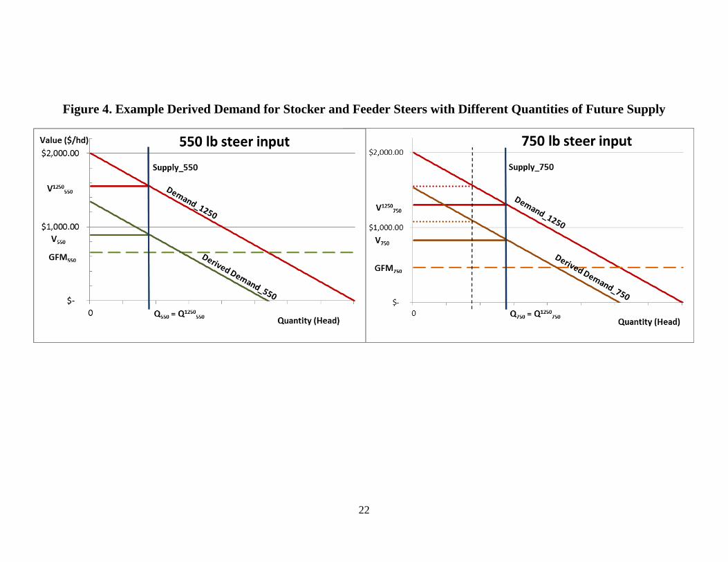
Figure 4 illustrates this point using separate derived demand markets for the 550 lb.

stockers and 750 lb. feeder steer inputs. The market for 550 lb. steers shown on the left is

identical to figure 3. However, the market shown in the panel on the right shows a larger supply

of 750 lb. feeder steers. Both input and output prices for the 750 lb. steer are lower relative to

the market conditions shown in figure 3 when a smaller quantity of steers was supplied. (For

reference, the supply curve and prices from figure 3 are shown by dashed lines in figure 4.)

Notice that the value of a 750 lb. feeder steer input in figure 4 is less than the value of the 550 lb.

stocker steer. This results directly from the lower expected live cattle price for the weight cohort

due to greater supply expectations.

This example clearly illustrates why a cross-section of prices for cattle of different sale

weights at a given point in time need not necessarily exhibit a downward-sloping price slide

relationship. Similar outcomes can be shown to result from differences in future demand for

slaughter steers. Because live cattle futures prices depend on expected supply and demand

6

conditions for a particular weight cohort of cattle, it will be important to link current cash

transactions to appropriate future price expectations in the empirical analysis.

III. Empirical Predictions

I use the two-input derived demand model to generate empirical predictions related to the

shape and dynamics of the price slide relationship. A mathematical representation of the model

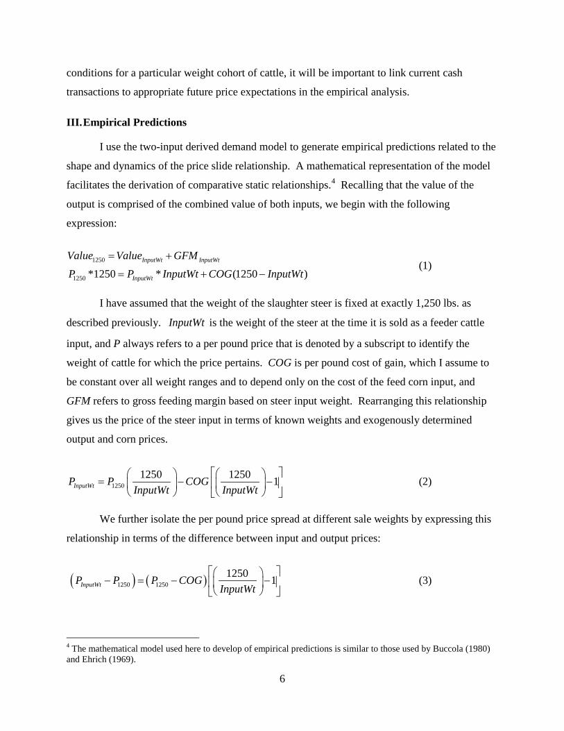
facilitates the derivation of comparative static relationships.4 Recalling that the value of the

output is comprised of the combined value of both inputs, we begin with the following

expression:

1250

1250 *1250 * (1250 )InputWt InputWt

InputWt

Value Value GFMP P InputWt COG InputWt

= +

= + − (1)

I have assumed that the weight of the slaughter steer is fixed at exactly 1,250 lbs. as

described previously. InputWt is the weight of the steer at the time it is sold as a feeder cattle

input, and P always refers to a per pound price that is denoted by a subscript to identify the

weight of cattle for which the price pertains. COG is per pound cost of gain, which I assume to

be constant over all weight ranges and to depend only on the cost of the feed corn input, and

GFM refers to gross feeding margin based on steer input weight. Rearranging this relationship

gives us the price of the steer input in terms of known weights and exogenously determined

output and corn prices.

12501250 1250 1InputWtP P COG

InputWt InputWt

= − −

(2)

We further isolate the per pound price spread at different sale weights by expressing this

relationship in terms of the difference between input and output prices:

( ) ( )1250 12501250 1InputWtP P P COG

InputWt

− = − −

(3)

4 The mathematical model used here to develop of empirical predictions is similar to those used by Buccola (1980) and Ehrich (1969).

7

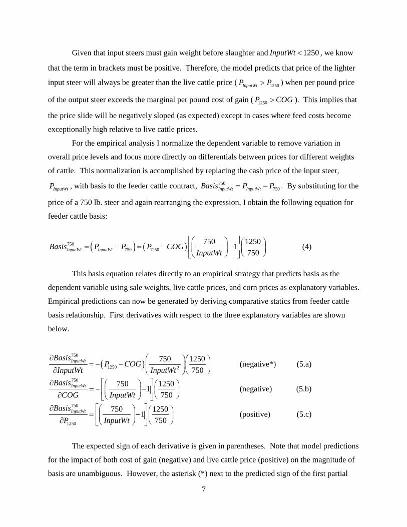
Given that input steers must gain weight before slaughter and 1250InputWt < , we know

that the term in brackets must be positive. Therefore, the model predicts that price of the lighter

input steer will always be greater than the live cattle price ( 1250InputWtP P> ) when per pound price

of the output steer exceeds the marginal per pound cost of gain ( 1250P COG> ). This implies that

the price slide will be negatively sloped (as expected) except in cases where feed costs become

exceptionally high relative to live cattle prices.

For the empirical analysis I normalize the dependent variable to remove variation in

overall price levels and focus more directly on differentials between prices for different weights

of cattle. This normalization is accomplished by replacing the cash price of the input steer,

InputWtP , with basis to the feeder cattle contract, 750750InputWt InputWtBasis P P= − . By substituting for the

price of a 750 lb. steer and again rearranging the expression, I obtain the following equation for

feeder cattle basis:

( ) ( )750750 1250

750 12501750InputWt InputWtBasis P P P COG

InputWt = − = − −

(4)

This basis equation relates directly to an empirical strategy that predicts basis as the

dependent variable using sale weights, live cattle prices, and corn prices as explanatory variables.

Empirical predictions can now be generated by deriving comparative statics from feeder cattle

basis relationship. First derivatives with respect to the three explanatory variables are shown

below.

( )750

1250 2

750 1250750

InputWtBasisP COG

InputWt InputWt∂ = − − ∂

(negative*) (5.a)

750 750 12501750

InputWtBasisCOG InputWt

∂ = − − ∂ (negative) (5.b)

750

1250

750 12501750

InputWtBasisP InputWt

∂ = − ∂ (positive) (5.c)

The expected sign of each derivative is given in parentheses. Note that model predictions

for the impact of both cost of gain (negative) and live cattle price (positive) on the magnitude of

basis are unambiguous. However, the asterisk (*) next to the predicted sign of the first partial

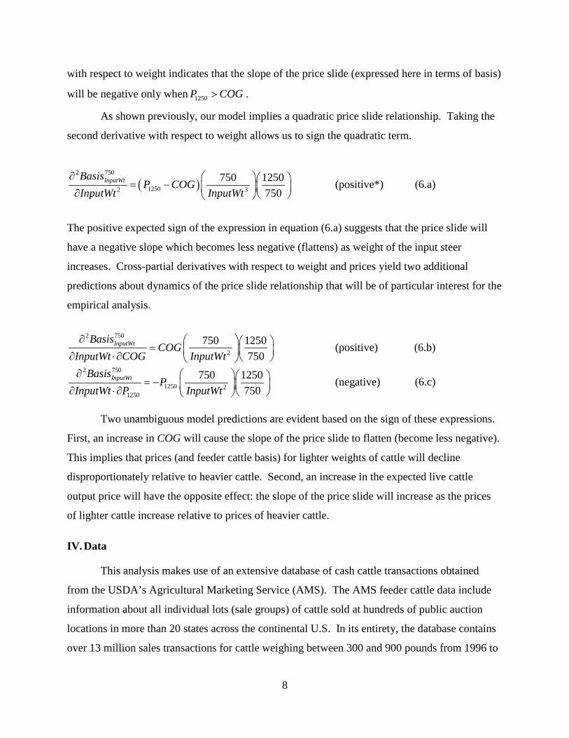
8

with respect to weight indicates that the slope of the price slide (expressed here in terms of basis)

will be negative only when 1250P COG> .

As shown previously, our model implies a quadratic price slide relationship. Taking the

second derivative with respect to weight allows us to sign the quadratic term.

( )2 750

12502 3

750 1250750

InputWtBasisP COG

InputWt InputWt∂ = − ∂

(positive*) (6.a)

The positive expected sign of the expression in equation (6.a) suggests that the price slide will

have a negative slope which becomes less negative (flattens) as weight of the input steer

increases. Cross-partial derivatives with respect to weight and prices yield two additional

predictions about dynamics of the price slide relationship that will be of particular interest for the

empirical analysis.

2 750

2

750 1250750

InputWtBasisCOG

InputWt COG InputWt∂ = ∂ ⋅∂

(positive) (6.b)

2 750

1250 21250

750 1250750

InputWtBasisP

InputWt P InputWt∂ = − ∂ ⋅∂

(negative) (6.c)

Two unambiguous model predictions are evident based on the sign of these expressions.

First, an increase in COG will cause the slope of the price slide to flatten (become less negative).

This implies that prices (and feeder cattle basis) for lighter weights of cattle will decline

disproportionately relative to heavier cattle. Second, an increase in the expected live cattle

output price will have the opposite effect: the slope of the price slide will increase as the prices

of lighter cattle increase relative to prices of heavier cattle.

IV. Data

This analysis makes use of an extensive database of cash cattle transactions obtained

from the USDA’s Agricultural Marketing Service (AMS). The AMS feeder cattle data include

information about all individual lots (sale groups) of cattle sold at hundreds of public auction

locations in more than 20 states across the continental U.S. In its entirety, the database contains

over 13 million sales transactions for cattle weighing between 300 and 900 pounds from 1996 to

9

2013. The cattle sold represent a variety of stages in the beef production process, from light

stockers to heavy feeders, although buyer information and intended use is not available.

A subset extracted from the larger AMS dataset has been used to conduct the preliminary

empirical analysis described in this working paper. The sample data contains 282,152

transactions from seven public auction locations in Kansas over a 10 year period. Each sales

transaction record in the dataset contains the date of sale, cash price, and several individual lot

characteristics. Lot characteristics about the group of cattle sold in each transaction include the

sales location, number of cattle in the group (lot size), average weight, and sex of the cattle

(steers, heifers, or bulls).

The AMS cash feeder cattle market data has been combined with CME futures price data.

Relevant cattle futures contracts were identified for each group of cattle sold, and prices were

linked to each transaction in the database. Sale date and average lot weight were used to

establish the future dates on which cattle in each sale lot would be predicted to attain weights of

750 and 1,250 pounds assuming a constant rate of weight gain. These weights were chosen

because they correspond to weight specifications for the feeder and live cattle futures contracts,

respectively.

As a specific example, consider a lot of cattle sold on 10/1/2012 with an average weight

of 550 lbs. Assuming average gain of 2 lbs. per day, these cattle would be expected to weigh

750 lbs. after 100 days on January 9, 2013. As of that date, the JAN2013 feeder cattle contract

would be next to expire (nearby contract) on 1/31/2013. The same group of cattle would be

expected to weigh 1,250 pounds after another 250 days ((1,250 lbs. – 750 lbs.) / 2 lbs./day) on

9/16/2013 when the OCT2013 live cattle contract would be next to expire on 10/31/2013. The

observed daily settlement prices for these contracts on 10/1/2013 determine the values of feeder

cattle and live cattle price variables for the cattle:

itFC750 = Price of JAN2013 feeder cattle contract on 10/1/2012 = $148.125 /cwt

itLC1250 = Price of OCT2013 live cattle contract on 10/1/2012 = $133.75 / cwt

These prices are subscripted for sale date t and individual lot i. They reflect the expected

future supply and demand conditions for a specific group of cattle described in the sales

transaction. In a broader sense, these are specific market price expectations for a single weight

cohort of cattle that are assumed to reach slaughter weight at the same time. For empirical

10

estimation, itFC750 is used as the current estimate of 750P (the expected future price of the group

of cattle at 750 lbs.) and itLC1250 is used as the current estimate of 1250P (the expected future

price of the group of cattle at 1,250 lbs.). Current basis is calculated using the feeder cattle

contract reference price of itFC750 for each cattle sales transaction as follows:

750it it itBasis Cash FC750= − (7)

The current price of the nearby corn contract, tCN0 , proxies for feed input costs in the

empirical model. For lighter weight animals, prices of deferred corn futures contracts (contracts

expiring after the nearby) might also be considered. However, the nearby contract price was

chosen as the best corn price expectation at all sale weights for two reasons: 1) remaining feed

input requirements are easily forecast in advance based on the average weight of the group of

cattle purchased, and 2) corn for grain is a storable commodity. Together, these imply that a

cattle buyer will always have the option of purchasing the expected feed corn requirement at the

same time as the cattle.

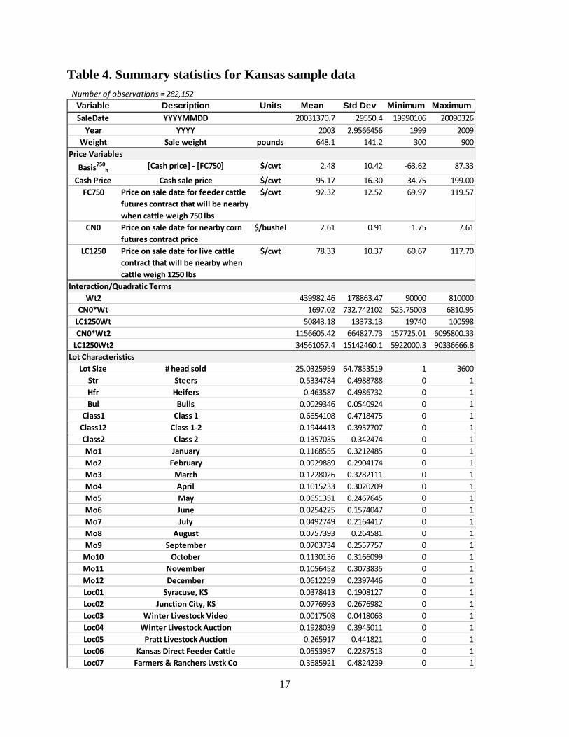
Table 4 displays summary statistics for the sample Kansas dataset that was used in the

empirical analysis. These data span a period from January 6, 1999 to March 26, 2009 and

include data for sale lots of feeder and stocker cattle weighing 300 to 900 pounds. The time

period also included substantial variation in the prices of feeder cattle ($69.97 to $119.57 per

cwt), live cattle ($60.67 to $117.70 per cwt), and corn ($1.75 to $7.61 per bushel). Feeder cattle

basis in the sample data ranged from a low of -$63.62 (when cash price was lower than FC750)

to a high of $87.33.

V. Estimation and Results

To test predictions developed from the two-input derived demand model, I estimate a

hedonic regression of feeder cattle basis. My analysis focuses primarily on the price relationship

between cattle basis and weight, as described previously. The basic regression specification in

Model 1 below describes this relationship and accommodates an expected quadratic shape for the

price slide.

Model 1: 750 2* *it it it itBasis a b Weight c Weight ε= + + +

11

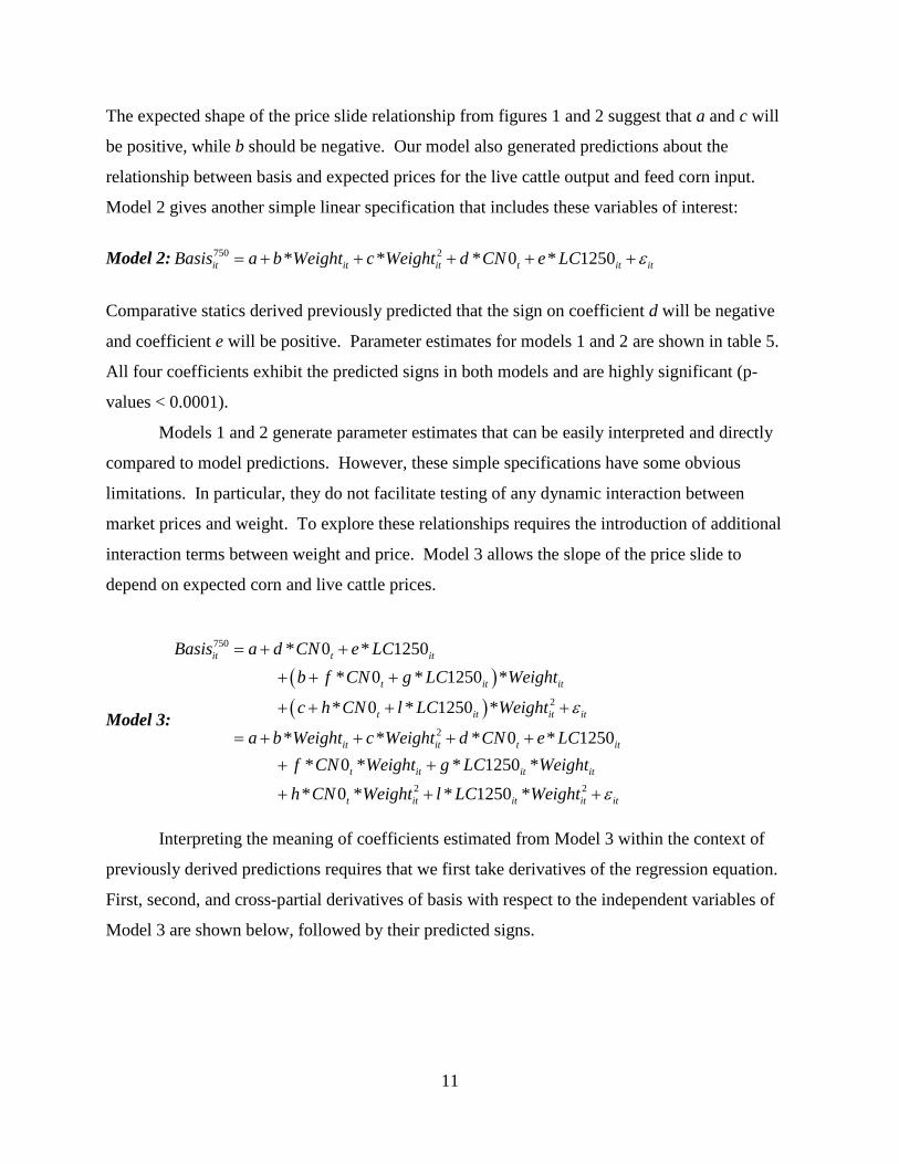
The expected shape of the price slide relationship from figures 1 and 2 suggest that a and c will

be positive, while b should be negative. Our model also generated predictions about the

relationship between basis and expected prices for the live cattle output and feed corn input.

Model 2 gives another simple linear specification that includes these variables of interest:

Model 2: 750 2* * * 0 * 1250it it it t it itBasis a b Weight c Weight d CN e LC ε= + + + + +

Comparative statics derived previously predicted that the sign on coefficient d will be negative

and coefficient e will be positive. Parameter estimates for models 1 and 2 are shown in table 5.

All four coefficients exhibit the predicted signs in both models and are highly significant (p-

values < 0.0001).

Models 1 and 2 generate parameter estimates that can be easily interpreted and directly

compared to model predictions. However, these simple specifications have some obvious

limitations. In particular, they do not facilitate testing of any dynamic interaction between

market prices and weight. To explore these relationships requires the introduction of additional

interaction terms between weight and price. Model 3 allows the slope of the price slide to

depend on expected corn and live cattle prices.

Model 3:

( )( )

750

2

2

* 0 * 1250 * 0 * 1250 *

* 0 * 1250 *

* * * 0 * 1250 * 0 * * 1250 *

it t it

t it it

t it it it

it it t it

t it it it

Basis a d CN e LCb f CN g LC Weight

c h CN l LC Weight

a b Weight c Weight d CN e LCf CN Weight g LC Weight

ε

= + +

+ + +

+ + + +

= + + + ++ +

2 2 * 0 * * 1250 *t it it it ith CN Weight l LC Weight ε+ + +

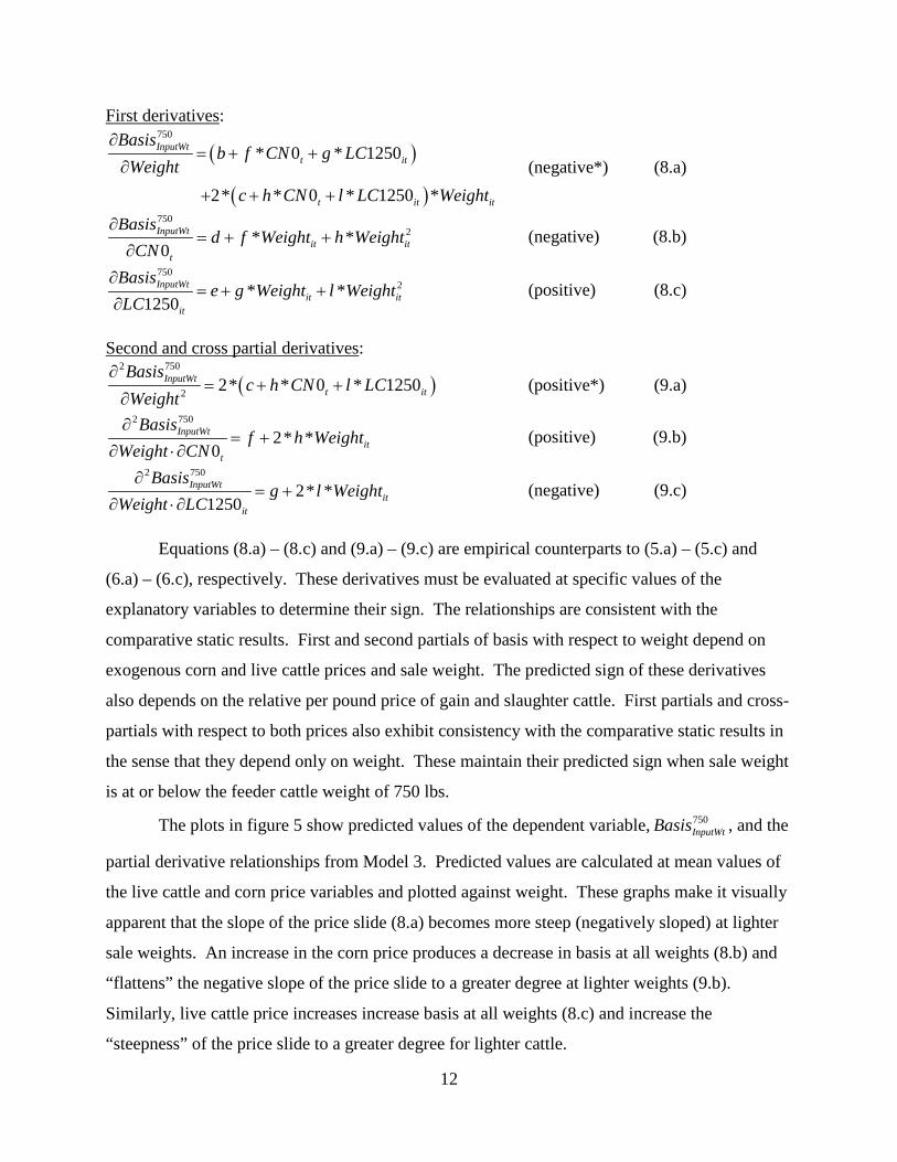
Interpreting the meaning of coefficients estimated from Model 3 within the context of

previously derived predictions requires that we first take derivatives of the regression equation.

First, second, and cross-partial derivatives of basis with respect to the independent variables of

Model 3 are shown below, followed by their predicted signs.

12

First derivatives:

( )

( )

750

* 0 * 1250

2* * 0 * 1250 *

InputWtt it

t it it

Basisb f CN g LC

Weightc h CN l LC Weight

∂= + +

∂

+ + +

(negative*) (8.a)

7502* *

0InputWt

it itt

Basisd f Weight h Weight

CN∂

= + +∂

(negative) (8.b)

7502* *

1250InputWt

it itit

Basise g Weight l Weight

LC∂

= + +∂

(positive) (8.c)

Second and cross partial derivatives:

( )2 750

2 2* * 0 * 1250InputWtt it

Basisc h CN l LC

Weight∂

= + +∂

(positive*) (9.a)

2 750

2* *0

InputWtit

t

Basisf h Weight

Weight CN∂

= +∂ ⋅∂

(positive) (9.b)

2 750

2* *1250

InputWtit

it

Basisg l Weight

Weight LC∂

= +∂ ⋅∂

(negative) (9.c)

Equations (8.a) – (8.c) and (9.a) – (9.c) are empirical counterparts to (5.a) – (5.c) and

(6.a) – (6.c), respectively. These derivatives must be evaluated at specific values of the

explanatory variables to determine their sign. The relationships are consistent with the

comparative static results. First and second partials of basis with respect to weight depend on

exogenous corn and live cattle prices and sale weight. The predicted sign of these derivatives

also depends on the relative per pound price of gain and slaughter cattle. First partials and cross-

partials with respect to both prices also exhibit consistency with the comparative static results in

the sense that they depend only on weight. These maintain their predicted sign when sale weight

is at or below the feeder cattle weight of 750 lbs.

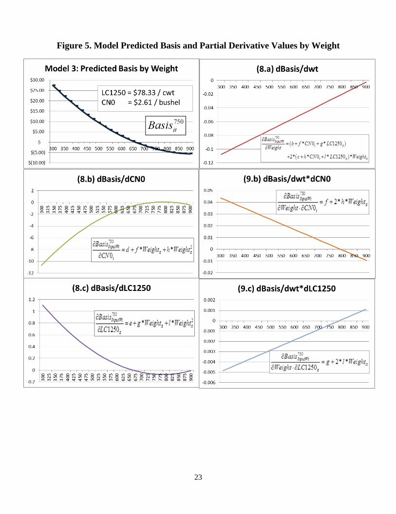
The plots in figure 5 show predicted values of the dependent variable, 750InputWtBasis , and the

partial derivative relationships from Model 3. Predicted values are calculated at mean values of

the live cattle and corn price variables and plotted against weight. These graphs make it visually

apparent that the slope of the price slide (8.a) becomes more steep (negatively sloped) at lighter

sale weights. An increase in the corn price produces a decrease in basis at all weights (8.b) and

“flattens” the negative slope of the price slide to a greater degree at lighter weights (9.b).

Similarly, live cattle price increases increase basis at all weights (8.c) and increase the

“steepness” of the price slide to a greater degree for lighter cattle.

13

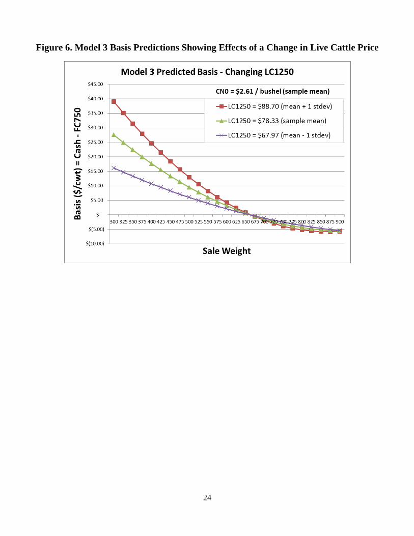
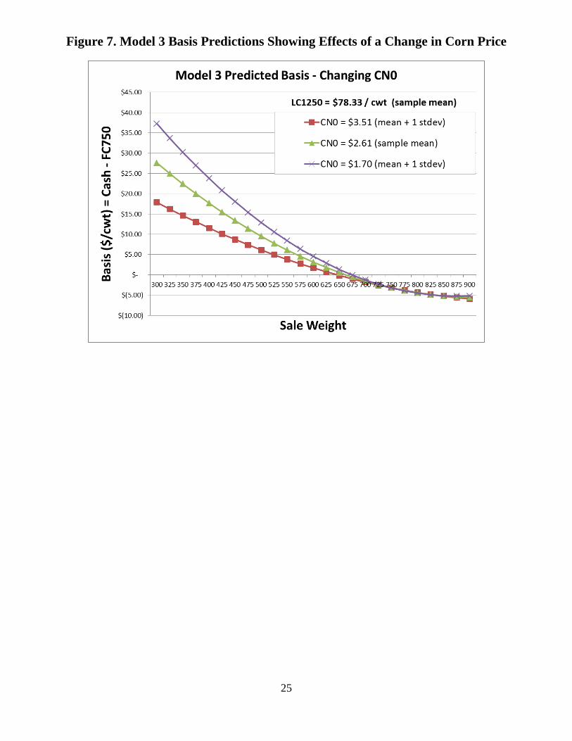
In order to more easily interpret and visualize the price slide dynamics, figures 6 and 7

plot predicted basis from Model 3 at different values of the corn an live cattle price. The price

slide shown in the middle of both figures plots basis predictions at the sample mean values of

both price variables (equivalent to figure 5). In figure 6, the corn price is held constant and two

additional predictions are plotted for the live cattle price at one standard deviation above and

below the sample mean of $78.33/cwt. Figure 7 holds live cattle price constant and plots

predictions for corn prices one standard deviation above and below the mean value of

$2.61/bushel. These figures clearly show the manner in which changes in live cattle and corn

prices make the price slide steeper or flatter and have larger impacts on the price slide at lighter

cattle weights.

Lot Characteristics

Several previous studies have demonstrated the importance of other lot characteristics in

determining feeder cattle prices and basis. I control for and test the significance of several lot

characteristics by adding them as additional explanatory variables in models 2 and 3. Table 5

displays estimates for the price and weight variables when other lot characteristics are included

as Model 2(o) and Model 3(o). Coefficients for individual lot characteristics are suppressed. A

comparison of estimated parameters from models with and without lot characteristics is

informative. Most notably, the inclusion of lot characteristics produces a considerable

improvement in the adjusted R-square for both models, suggesting that these factors are indeed

important basis determinants. Further, the inclusion of lot characteristics does not cause

appreciable change in the values of any of the price-weight coefficients.

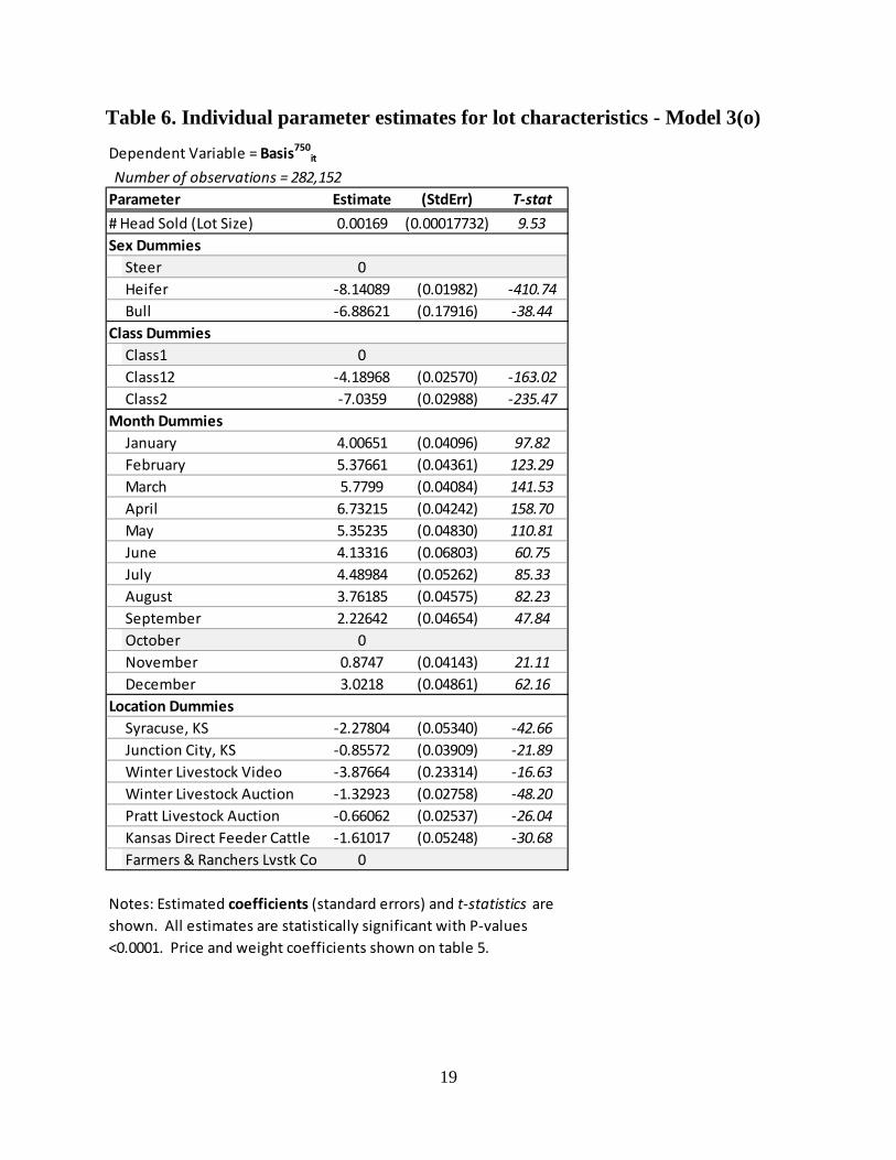
Coefficients for the individual lot characteristic variables from the Model 3(o)

specification are displayed separately in table 6. All of these estimates exhibit strong statistical

significance, which is not surprising in light of the large number of observations. The sign of the

coefficient on lot size is consistent with many previous studies (for example Dhuyvetter and

Schroeder, 2000), which have shown that larger groups of cattle sell at a premium compared to

smaller lots. Dummy variables were included for four additional characteristics: sex, class,

month, and location. The estimates suggest that buyers pay a premium for steers relative to

heifers or bulls and for cattle grading at class 1. Monthly dummy variables capture seasonal

price differences and show that basis is lowest for feeder cattle that are sold in the fall months.

This is consistent with previous research and also consistent with the notion that a large supply

14

of spring calves results in a large supply of fall stocker cattle. Location dummies reveal that

basis also differs based on where the cattle are sold. This might result from geographic price

differences as well as from differences in the type of cattle that are sold at different auction

locations.

VI. Conclusions and Future Research

The research presented in this working draft has demonstrated that empirical

relationships between price and weight are consistent with predictions derived from a simple

two-input derived demand model. Dynamics of the cattle price slide are clearly linked to

changing conditions in the markets for corn feed inputs and live cattle outputs. Further, these

relationships depend on future expectations of prices for cattle at different sale weights.

Information about expected future market conditions for specific groups of cattle was

incorporated by identifying appropriate futures contract prices.

The preliminary empirical analysis presented here suggests many possible areas for

future exploration. For example, several explanatory variables could potentially be added to the

model. These might include proxies for pasture feed inputs (ex., Palmer drought index), cattle

inventory numbers, fuel costs, and recent feedlot profit margins. I also plan to consider the

potential for additional dynamic interactions between the price slide and market or lot

characteristics. Future empirical analysis will include more extensive treatment of

contemporaneous corn and live cattle price relationships. In particular, I will explore whether

high corn prices in recent years may have caused the price slide relationship to invert at certain

points in time.

Most obviously, the analysis will be expanded to include a vast AMS database of feeder

cattle transactions. This introduces regional variation in price slide dynamics that might stem

from proximity to corn production and feedlot facilities or from regional differences in

production practices and types of animals sold. Expanding the dataset will also introduce

additional intertemporal variation by the inclusion of recent years with high and variable prices.

I will look to exploit this substantial variation and contribute to the understanding of price slide

dynamics.

15

References

Anderson, J.D. and J.N. Trapp. 2000. “The Dynamics of Feeder Cattle Market Responses to Corn Price Change.” Journal of Agricultural and Applied Economics 32: 493-505.

Buccola, S.T. 1980. “An Approach to the Analysis of Feeder Cattle Price Differentials.” American Journal of Agricultural Economics 62: 574-580.

Dhuyvetter, K.C. and T.C. Schroeder. 2000. “Price-Weight Relationships for Feeder Cattle.” Canadian Journal of Agricultural Economics 48: 299-310.

Dhuyvetter, K.C., K. Swanser, T. Kastens, J. Mintert and B. Crosby. 2008. “Improving Feeder Cattle Basis Forecasts.” Western Agricultural Economics Association Selected Paper.

Ehrich, R.L. 1969. “Cash-Futures Price Relationships for Live Beef Cattle.” American Journal of Agricultural Economics 51: 26-40.

Friedman, M. 1962. Price Theory. Aldine Publishing Co., Chicago, IL. Marsh, J.M. 1985. “Monthly Price Premiums and Discounts Between Steer Calves and

Yearlings.” American Journal of Agricultural Economics 67: 307-314.

Schroeder, T.C., J.R. Mintert, F. Brazle and O. Grunewald. 1988. “Factors Affecting Feeder Cattle Price Differentials.” Western Journal of Agricultural Economics 13: 71-81.

16

Table 1. Example feed cost calculations for two weights of the steer input

Table 2. Example derived steer input values and prices

Table 3. Summary of example steer prices by weight

Feeder StockerOutput (slaughter) weight 1250 1250 lbs- Input Weight 750 550 lbsGain Required 500 700 lbsx Corn Conversion 7 7 Corn Input (lbs) 3,500 4,900 lbs÷ corn bushels / lb 56 56 Corn Input (bushels) 62.5 87.5 bushelsx Corn Price ($/bushel) 7.50$ 7.50$ per bushelGross Feeding Margin (GFM) 468.75$ 656.25$ per headCost of Gain (COG) 0.94$ 0.94$ per lb

Price_LC1250 1.24$ 1.24$ per lbx Weight_1250 1250 1250 lbsSlaughter value 1,550.00$ 1,550.00$ $/hd- GFM 468.75$ 656.25$ $/hdSteer Input Value (derived) 1,081.25$ 893.75$ $/hd÷ steer input weight 750 550 lbsSteer Input Price (derived) 1.44$ 1.63$ per lb

Steer type Weight Price ValueSlaughter 1250 1.24$ 1,550.00$ Feeder 750 1.44$ 1,081.25$ Stocker 550 1.63$ 893.75$

17

Table 4. Summary statistics for Kansas sample data

Number of observations = 282,152Variable Description Units Mean Std Dev Minimum MaximumSaleDate YYYYMMDD 20031370.7 29550.4 19990106 20090326

Year YYYY 2003 2.9566456 1999 2009Weight Sale weight pounds 648.1 141.2 300 900

Price VariablesBasis750

it [Cash price] - [FC750] $/cwt 2.48 10.42 -63.62 87.33

Cash Price Cash sale price $/cwt 95.17 16.30 34.75 199.00FC750 Price on sale date for feeder cattle

futures contract that will be nearby when cattle weigh 750 lbs

$/cwt 92.32 12.52 69.97 119.57

CN0 Price on sale date for nearby corn futures contract price

$/bushel 2.61 0.91 1.75 7.61

LC1250 Price on sale date for live cattle contract that will be nearby when cattle weigh 1250 lbs

$/cwt 78.33 10.37 60.67 117.70

Interaction/Quadratic TermsWt2 439982.46 178863.47 90000 810000

CN0*Wt 1697.02 732.742102 525.75003 6810.95LC1250Wt 50843.18 13373.13 19740 100598CN0*Wt2 1156605.42 664827.73 157725.01 6095800.33

LC1250Wt2 34561057.4 15142460.1 5922000.3 90336666.8Lot Characteristics

Lot Size # head sold 25.0325959 64.7853519 1 3600Str Steers 0.5334784 0.4988788 0 1Hfr Heifers 0.463587 0.4986732 0 1Bul Bulls 0.0029346 0.0540924 0 1

Class1 Class 1 0.6654108 0.4718475 0 1Class12 Class 1-2 0.1944413 0.3957707 0 1Class2 Class 2 0.1357035 0.342474 0 1Mo1 January 0.1168555 0.3212485 0 1Mo2 February 0.0929889 0.2904174 0 1Mo3 March 0.1228026 0.3282111 0 1Mo4 April 0.1015233 0.3020209 0 1Mo5 May 0.0651351 0.2467645 0 1Mo6 June 0.0254225 0.1574047 0 1Mo7 July 0.0492749 0.2164417 0 1Mo8 August 0.0757393 0.264581 0 1Mo9 September 0.0703734 0.2557757 0 1

Mo10 October 0.1130136 0.3166099 0 1Mo11 November 0.1056452 0.3073835 0 1Mo12 December 0.0612259 0.2397446 0 1Loc01 Syracuse, KS 0.0378413 0.1908127 0 1Loc02 Junction City, KS 0.0776993 0.2676982 0 1Loc03 Winter Livestock Video 0.0017508 0.0418063 0 1Loc04 Winter Livestock Auction 0.1928039 0.3945011 0 1Loc05 Pratt Livestock Auction 0.265917 0.441821 0 1Loc06 Kansas Direct Feeder Cattle 0.0553957 0.2287513 0 1Loc07 Farmers & Ranchers Lvstk Co 0.3685921 0.4824239 0 1

18

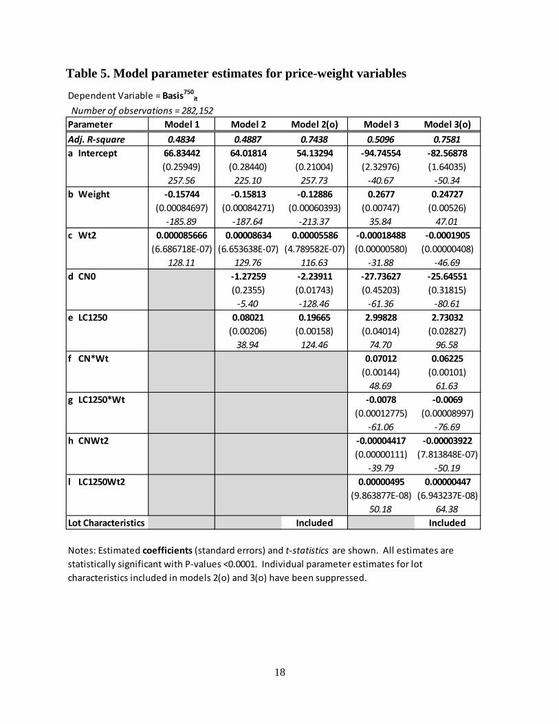
Table 5. Model parameter estimates for price-weight variables

Dependent Variable = Basis750it

Number of observations = 282,152Parameter Model 1 Model 2 Model 2(o) Model 3 Model 3(o)Adj. R-square 0.4834 0.4887 0.7438 0.5096 0.7581a Intercept 66.83442 64.01814 54.13294 -94.74554 -82.56878

(0.25949) (0.28440) (0.21004) (2.32976) (1.64035)257.56 225.10 257.73 -40.67 -50.34

b Weight -0.15744 -0.15813 -0.12886 0.2677 0.24727(0.00084697) (0.00084271) (0.00060393) (0.00747) (0.00526)

-185.89 -187.64 -213.37 35.84 47.01c Wt2 0.000085666 0.00008634 0.00005586 -0.00018488 -0.0001905

(6.686718E-07) (6.653638E-07) (4.789582E-07) (0.00000580) (0.00000408)128.11 129.76 116.63 -31.88 -46.69

d CN0 -1.27259 -2.23911 -27.73627 -25.64551(0.2355) (0.01743) (0.45203) (0.31815)

-5.40 -128.46 -61.36 -80.61e LC1250 0.08021 0.19665 2.99828 2.73032

(0.00206) (0.00158) (0.04014) (0.02827)38.94 124.46 74.70 96.58

f CN*Wt 0.07012 0.06225(0.00144) (0.00101)

48.69 61.63g LC1250*Wt -0.0078 -0.0069

(0.00012775) (0.00008997)-61.06 -76.69

h CNWt2 -0.00004417 -0.00003922(0.00000111) (7.813848E-07)

-39.79 -50.19l LC1250Wt2 0.00000495 0.00000447

(9.863877E-08) (6.943237E-08)50.18 64.38

Lot Characteristics Included Included

Notes: Estimated coefficients (standard errors) and t-statistics are shown. All estimates are statistically significant with P-values <0.0001. Individual parameter estimates for lot characteristics included in models 2(o) and 3(o) have been suppressed.

19

Table 6. Individual parameter estimates for lot characteristics - Model 3(o)

Dependent Variable = Basis750it

Number of observations = 282,152Parameter Estimate (StdErr) T-stat# Head Sold (Lot Size) 0.00169 (0.00017732) 9.53Sex Dummies

Steer 0Heifer -8.14089 (0.01982) -410.74Bull -6.88621 (0.17916) -38.44

Class DummiesClass1 0Class12 -4.18968 (0.02570) -163.02Class2 -7.0359 (0.02988) -235.47

Month DummiesJanuary 4.00651 (0.04096) 97.82February 5.37661 (0.04361) 123.29March 5.7799 (0.04084) 141.53April 6.73215 (0.04242) 158.70May 5.35235 (0.04830) 110.81June 4.13316 (0.06803) 60.75July 4.48984 (0.05262) 85.33August 3.76185 (0.04575) 82.23September 2.22642 (0.04654) 47.84October 0November 0.8747 (0.04143) 21.11December 3.0218 (0.04861) 62.16

Location DummiesSyracuse, KS -2.27804 (0.05340) -42.66Junction City, KS -0.85572 (0.03909) -21.89Winter Livestock Video -3.87664 (0.23314) -16.63Winter Livestock Auction -1.32923 (0.02758) -48.20Pratt Livestock Auction -0.66062 (0.02537) -26.04Kansas Direct Feeder Cattle -1.61017 (0.05248) -30.68Farmers & Ranchers Lvstk Co 0

Notes: Estimated coefficients (standard errors) and t-statistics are shown. All estimates are statistically significant with P-values <0.0001. Price and weight coefficients shown on table 5.

20

Figure 1. Example value, price, and feed cost calculations by steer input weight

Figure 2. Example calculations with reduced corn price

Value_1250 = $1,550.00 P_1250 = LC1250 = $1.24/lb Corn Price = $7.50/bu

Price slide ($/lb)

Value ($/ hd)

Value_750 = $1,081.25 Price_750 = $1.44/lb.

P_1250 = LC1250 = $1.24/lb Corn Price = $3.50/bu

GFM ($7.50/bu) # of days needed to reach 1250 lbs.

Value_1250 = $1,550.00

Value ($/ hd)

Price slide ($/lb) Value_750 = $1,331.25 Price_750 = $1.78/lb

GFM ($3.50/bu)

# of days needed to reach 1250 lbs.

21

Figure 3. Example Derived Demand Market for Input Steers at 550 and 750 lb. Sale Weights

22

Figure 4. Example Derived Demand for Stocker and Feeder Steers with Different Quantities of Future Supply

23

Figure 5. Model Predicted Basis and Partial Derivative Values by Weight

24

Figure 6. Model 3 Basis Predictions Showing Effects of a Change in Live Cattle Price

25

Figure 7. Model 3 Basis Predictions Showing Effects of a Change in Corn Price