Dynamics of a Protected Housing Market:

The Case of Switzerland

Karol Jan Borowiecki

TEP Working Paper No. 1010

October 2011

Trinity Economics Papers Department of Economics Trinity College Dublin

1

Dynamics of a Protected Housing Market:

The Case of Switzerland

Karol Jan Borowiecki

Abstract

This study posits that there may be a strong relationship between the high degree of protectionism of

the Swiss housing market and its stability. The article provides an overview of the Swiss housing

policies that, it is argued, are highly conservative in the context of an international comparison. The

stability of the Swiss housing economy is empirically tested. Based on the time period from 1990 to

2009, in which two substantial crises occurred, house prices and construction activity are modeled. The

emerging results, which are admittedly based on a very short time series, are nonetheless consistent

with previous theoretical and empirical research. Furthermore, the findings indicate that the Swiss

housing economy operates in accordance with fundamentals. Based on a tentative approach that

measures the occurrence of the crisis with annual indicator variables, no effects of the crises on the

Swiss housing market can be detected.

Keywords: Housing Demand, Housing Supply and Markets

JEL Classification: R21, R31

Contact: Trinity College Dublin, Department of Economics, Dublin 2, Ireland. E-Mail:

borowiek@tcd.ie. The author is grateful to Clemens Struck for his assistance and technical advice

during this project. Helpful suggestions have been also received from Kenneth Gibb and anonymous

referees.

2

1. Introduction

The recent global financial crisis was unforeseen, of unexpected global dimensions and, to

some extent, caused by the collapse of the United States housing bubble. This was not,

however, the first real estate crisis in the U.S. and neither was America the only country

where a national property crisis coincided with the distress of the entire economy. Property

crises are notoriously recurring and leveraging of economic downturns. The recent financial

crisis led to distress in most developed economies and in turn causing a significant drop in the

price of property. There are however exceptions. The Swiss housing economy is such an

exception and remains mostly unaffected by the recent ‘Great Recession’.

That level of robustness of the Swiss housing market is possibly a result of its very high

protectionism when compared internationally. The market is not easily accessible for foreign

investors and it provides several disincentives for domestic speculators. Due to rigid taxation

of home owners and conservative mortgage lending schemes the market is dominated by

tenants. The formation of the Swiss housing market was shaped by several factors most

significant of which was a substantial real estate economy crisis in the early 90’s which

stimulated the introduction of several protective regulations and practices. One question

which is of potential interest for today’s policy-makers is how well is the Swiss housing

sector protected from economic turbulence? This is the question which is being addressed in

this study. Furthermore, a summary of the Swiss housing policies that might have contributed

to the stability of the market is provided.

The relationship between the degree of protectionism and house price dynamics is not

straightforward. Ideally, one would want to conduct an international comparison of the degree

of protectionism of national housing markets and study its role in housing value stability.

Such an assessment is not, however, possible due to the lack of appropriate indices. As an

approximation for the level of regulatory protection the Property Rights Index, provided by

Global Property Guide (2011), is used. The suggested index is a sub-component of the Index

of Economic Freedom and it indicates the degree to which a country’s laws protect private

property rights, as well as the degree to which its government enforces those laws. The

association between the Property Rights Index and changes in European house prices over 10

years using the latest data available (as recorded by Global Property Guide, 2011) is

illustrated in Figure 1. The emerging picture implies a strongly negative relationship with a

correlation coefficient equal to -0.73. The more regulated a national housing economy is a

lower increase in house prices can be expected. Switzerland has the second lowest house

price growth over the last 10 years and its Property Rights Index takes the highest value (i.e.

90 out of 100).

This study also provides an estimation of a model of the Swiss housing price and

3

construction activity in order to investigate their interdependence as well as to identify their

main drivers. The econometric analysis allows for further investigation of whether the

economy is in accordance with fundamentals. The analysis is based on annual observations

from 1990 to 2009. The time period under investigation is particularly interesting as it

facilitates some new understanding of the performance of a protected and conservative market

at a time of some turbulence in international property markets. We construct a vector

autoregressive model and find that house prices are positively related with construction price,

working age population as well as GDP and are negatively associated with interest rates.

Construction activity is stimulated by the size of the working age population and GDP; it

discloses, however, a negative relationship with construction price and interest rates. The

results are in accordance with theoretical as well as recent empirical research. It can further be

concluded that the Swiss house price is in accordance with fundamentals. Furthermore, the

recent financial crisis has barely had any effect on the Swiss housing market. Nonetheless, the

econometric results have to be interpreted with caution as it is difficult to obtain reliable

estimates for a short time period, especially if variables are interdependent with their own

lags and the lags of other variables. In addition the detection of stationarity of variables can

often not be conducted with high accuracy.

The remainder of this article is organized as follows. In the next section, the Swiss

housing market is presented and compared with other national housing markets. In the third

section, related literature is discussed and in the fourth the data sources are disclosed and the

methodological approach introduced. In the fifth section, the empirical findings are presented

and in the last section, concluding remarks are provided.

2. The Swiss Housing Economy in an International Context

As can be seen in Figure 2, the Swiss housing economy has been in an upward trend since the

release of the major Swiss house price index (SWX IAZI Private Real Estate Price Index).1

Furthermore, there some indication of a 25-year-long housing price cycle can be detected.

The greatest increases can be observed during the Swiss construction boom of the early

eighties, which was further leveraged in 1987 by the introduction of the Swiss Interbank

Clearing System that led to a substantial money supply extension. Nonetheless, the bubble

burst when the speculative belief of the market was confronted with the unexpected economic

downturn of the early nineties.

Those events have forced the Swiss policy makers to introduce urgent sanctions on real

estate speculation. While the timing of those sanctions has been criticized by some, their

1 For a discussion of earlier house price changes and overview of historical developments in Swiss

housing policy since World War II refer to Lawrance (1996).

4

long-term benefit is mirrored by the extraordinary stability of the housing economy in

Switzerland during the recent financial crisis. A 5-year blocking period was introduced for the

sale of non-agricultural land and buildings, more stringent regulations for pension fund

investors and stricter mortgage underwriting criteria. The taxation of real estate transaction

has been tightened and relatively high progressive taxes on realized capital gains were also

introduced. Those fiscal burdens are negatively related to the duration of property ownership

which is another factor that mitigates speculation. In addition, the Swiss financial center

implemented changes in governance, risk management and compliance. In particular, Swiss

banks became more cautious and conservative about their credit lending. Properties would be

financed up to a maximum of 80 per cent of their value, if the cost of owning did not exceed

one third of a household’s gross income (Bourassa et al., 2009).

The Swiss housing market is also well isolated from foreign investments. The

acquisition of residential properties in Switzerland by foreigners is restricted due to the ‘Lex

Koller’ legislation. The significance of this legislation became visible after it was recently

loosened, allowing for the acquisition of holiday homes by foreigners and resulting in

substantial price inflation in this sub-market. Another remarkable characteristic of the Swiss

housing economy is its dominance by tenants. In this extent “(t)he Swiss housing market

differs considerably from what one might expect based on the economic conditions of one of

the world’s wealthiest nations” (Werczberger, 1997, p. 337). Switzerland’s home ownership

rate at 34.6 per cent is the lowest among developed countries. As proposed by Bourassa and

Hoesli (2006) this is primarily caused by high house prices relative to rents and relative to

household incomes and wealth. Furthermore, discriminatory taxation of home owners and

regulations that favor tenants provide further disincentives for house buyers. In comparison

with the US, the Swiss system of income taxation is much less favorable to home ownership

(Bourassa et al., 2009). For example, for annual taxation owners of residential properties must

include to their income imputed rent, which constitutes 70 per cent of market rent. A further

distinct difference from the US housing economy is the nature of the housing stock. As

outlined by Bourassa et al. (2009), the share of multi-family houses accounts for around 70

per cent, which is twice as high as in the US, while the share of single-family houses,

accounting for 23 per cent of the Swiss housing stock, is only fractional compared with the

US (60 per cent). Obviously, the availability of the former type of housing stock plays an

important role in the flat rental market, whereas single-family houses constitute a much less

attractive category for rentals.

Figure 3 presents an international comparison of risk-return profiles for a selection of

seventeen countries.2 It becomes obvious that Switzerland, Japan and Germany expose the

2 Figure 2 has to be compared under the caveat that data on residential property prices are not strictly

5

lowest standard deviation of house prices among all studied countries. If countries with

positive growth rates in house price are considered, Switzerland clearly has the lowest level

of volatility. Given its risk profile, it provides a high annual return of around 2.6 per cent.

3. Literature Overview

A standard approach in the literature expressed by Poterba (1984) is to model the housing

market as an asset market. Case and Shiller (1990) notice, however, that the housing market is

not very efficient and that it is possible to forecast house prices. They find that a change in

real housing prices predicts its own change in the following year. Additional evidence in that

respect comes from Malpezzi (1999) who rejects the random walk hypothesis for house

prices.3

Intuitively, housing demand is negatively related to interest rates as higher interest

rates make investing in houses (by borrowing) more expensive and other interest-bearing

assets more attractive. Viewed through the lens of asset pricing, an increase in mortgage

interest payments lowers future returns on a house and, hence, lowers demand for this asset

leading to a fall in prices. The influence of interest rates on house prices is, among other

factors, formalized under the label of the user costs of housing. Employing this concept,

Poterba (1984) argues that inflation – a substantial part of the real interest rate - reduces the

effective cost of home ownership.

Kahn (2008, 2009) attributes the change in house prices to productivity growth. The

channel through which productivity growth affects house prices is income. Productivity

growth increases lead to current income growth and, if persistent, raise expectations for

higher future income. As a consequence, the demand for housing rises and this increases the

price of housing ceteris paribus.

On the demand side, it is important to incorporate the idea that demographics could

substantially drive housing demand. Furthermore, housing demand rises sharply between the

ages of 20 and 30 and declines slowly after the age of 40 (for example, Levin et al., 2009).

Certain age cohorts (below 20 and above some upper threshold) have, therefore, little impact

on the demand for housing.

On the supply side, construction activities depend on the profitability of house

building and, hence, should be positively correlated with the level of real house prices.

Because the market participants are forward looking, house prices should contain some (if not

all) information about future developments in the market, including information about future

construction activities. In an analysis of the UK housing market, Ball (2010) finds that

comparable across countries due to differences in definitions. 3 See also HM Treasury (2003): ‘Housing, Consumption and EMU’ for a detailed review.

6

regulatory controls on the supply of housing results in the low responsiveness of housing

supply to changes in market activity. It is likely that the sluggishness in the market causes a

change in current housing supply to be correlated with past changes in supply. Remaining

influences on the profitability of new house building include the costs of house building.

Housing demand is therefore defined by the following equation:

D=f(P, Y, r, XD), (1)

where housing demand (D) is a function of real house prices (P), real income (Y), real interest

rates (r) and a vector of other demand factors (XD) like demographics or expected return on

housing.

S=f(P, XS) (2)

Equation (2) states that the housing supply is a function of real house prices and a number of

factors (XS) that influence the profitability of house building like construction costs. We

assume throughout the paper that the housing market is in equilibrium and derive from

Equations (1) and (2) an expression for real house prices:

P=f(Y, r, XD, XS) (3)

The empirical research in this area has a strong US focus. Poterba (1991) examines

the changes in the construction costs, demographic factors and the real, after-tax cost of home

ownership as possible determinants of shifts of demand and supply in the housing market.

Case and Shiller (1990) study the persistence of price changes for single-family homes in

U.S. cities. More recent research has investigated the markets of other countries. Examples of

these studies are Meese and Nancy (2003) for the French market and Meen (2002) who

looked at the British market. Cross-country studies usually focus on advanced economies, see

Englund and Ioannides (1997) among others. For the Swiss housing market the list of

academic publications is rather short. Bourassa and Hoesli (2006) identify the key

determinants of the Swiss home ownership rate. Borowiecki (2009) models Swiss house

prices and investigates the over-valuation of the market while Degen and Fischer (2010)

investigate the impact of immigration on Swiss house prices.

4. Data and Methodology

4.1 Data Description

7

To model house prices we follow several articles in the literature that model housing supply

and demand. Assuming that the market is in a state of equilibrium (i.e. supply equals demand),

we regress house prices and construction activities on a set of independent variables that have

been identified as drivers of supply and demand in previous studies. We also include lagged

values of house prices and construction activities as independent variables, since these lags

are often found to contain predictive power for current house price growth. Our measure for

house price growth is derived from IAZI Swiss Exchange Private Real Estate Price Index.4

The index is based on information from banks, insurers and pension funds on actual changes

of ownership. The house price index covers more than 60 per cent of the property transactions

concluded in Switzerland. Because we are particularly interested in the real fluctuations in the

housing market, we deflate our variables with the CPI deflator. As a proxy for construction

activities we use the number of apartments under construction each year.5 Since the Swiss

home ownership ratio is very low in an international context, apartments play a relatively

large role and should therefore account for a substantial part of the residential property price

variation. The data for apartment construction is obtained from the Swiss National Bank

(SNB). We further augment our model with a couple of independent variables.

First, we include real domestic interest rates. Interest rates change the user cost of

housing as discussed in the previous section and alter the attractiveness of investing in

interest-bearing assets. For the key interest rate we use the Swiss discount rate.6 In order to

account for demographic factors that could potentially drive house prices through the demand

channel, we employ working age population (20-64); that is the age group of the overall

population that has potentially the highest influence in determining housing demand. To

incorporate the house price dependency on income and expectations of future income we

include both, the development of Swiss GDP relative to the rest of the world and the

unemployment rate as a measure of welfare. Using GDP as share of the world instead of

regular GDP has the advantage that it captures relative movements in income. This is

important since the underlying theories point to forward looking consumers that make

decisions based on their expectations. Borrowing and lending by consumers, however,

increasingly depends on the performance of a country relative to the world. This is caused by

better access to international asset markets and employment of international investment

opportunities for the benchmark of the domestic investor. If, for example, other countries are

4 The International Securities Identifying Number of this index is CH0030532342. From now on we

refer to this index as ‘house prices’. 5 Records on construction of houses are not available. Data availability also restricts us from using a

more sophisticated measure, such as the annual change in the number of square meters in residential

property. 6 Data was obtained from the Swiss National Bank statistics. Refer also to Table A1 in the Appendix

for data sources of all remaining variables.

8

growing faster, then capital would rather flow abroad instead of being invested domestically.

Consequently, the inclusion of a measure of GDP relative to the world is required as it would

capture these considerations better than an absolute GDP measure could. Unemployment,

GDP and CPI data come from the IMF WEO database which collects its information from the

national authorities.

The housing supply is expected to be positively related to the profitability of house

building and, hence, positively correlated to the level of real house prices. This relationship

could, however, be distorted in the short-run due to the sluggish nature of housing supply.

Hence, we also include two lags of past changes in construction activities in our regressions.

Remaining influences on the profitability of new house building include the construction cost.

These costs are subsumed in the lagged house prices (that capture changes in the prices of

land) and in an additional variable that we include - the CPI adjusted change in construction

prices. As a construction price index we use the construction cost index for residential

buildings provided by the Swiss National Bank. The selected data set covers the time period

from 1990 to 2009 on an annual basis. Table 1 gives a description of the time series.

4.2 Empirical Setup

The results from unit root testing of the underlying variables, which are based on the

augmented Dickey-Fuller (ADF) and Phillips-Perron (PP) tests, are presented in Table 2. The

overall results are fairly concurrent with previous empirical findings. Both tests provide some

indication that all variables are stationary, except interest rates and population growth.7 Due

to the relatively low number of observations stationarity tests lack power. It is, therefore,

difficult to distinguish between stationary and non-stationary time periods. If a longer data

series of population was employed, the tests would suggest integration of order one. Building

on those results and considering recent empirical research (e.g. Oikarinen 2007) we assume

real interest rates to be integrated of order zero. All other variables we assume to be

integrated of order one and hence we employ their growth rates. Nonetheless, the

interpretation of the relationship between real interest rates and house prices should come

with some caution since the real interest rates have fallen over time and, thus, exhibit a time

trend. Both the augmented Dickey-Fuller and the Philipps-Perron test indicate non-

stationarity of the real interest rates. This is not so much of a problem in the regression with

the change in construction activities as a dependent variable - because this variable is highly

stationary. But due to the weak stationarity of the change in the CPI adjusted change in house

prices, the estimates might contain some noise because of the underlying time trends.

We complement the above analysis with an investigation of breaks in the housing price

7 For population growth the null hypothesis that the variable contains a unit root is however somewhat

close to not being rejected (p-value<0.16).

9

series and compute an innovational outlier unit root test that allow for two structural breaks

(see Clemente et al., 1998). The emerging picture is presented in Appendix 2. The series is

found to contain two breaks at years 1994 and 2005.8 The structural break at 1994 can

presumably be explained by the introduction of construction subsidies by Swiss authorities in

response to the housing crisis at the start of 1990. The subsidies to the extent of over 6bn

USD led to a construction boom and ended with a massive over-supply around the year 1994

(Credit Suisse, 2000). The structural break at 2005 presumably coincides with the Free

Movement of Persons from the EU/EFTA, which was introduced three years earlier. With the

facilitation of migration, there resulted large migration inflows into Switzerland, leading to

population growth of up to around 1 per cent. None of the structural breaks coincide with the

recent global recession, which provides some indication of the robustness of the Swiss

housing economy. Given that the data set ends in 2009, this, however, only provides tentative

evidence. In addition, based on the conducted unit root test we can conclude the necessity of

including all regressions’ additional control variables that take account of the structural

breaks.

As some of the variables in our system are integrated of the same order I(1), testing for

cointegration may be desirable. The likelihood ratio trace test fails however to reject the null

hypothesis of no cointegration. Similarly, the maximum eigenvalue statistic cannot reject the

null hypothesis of no cointegration. As the results point to the absence of a cointegration

relationship, we refrain from constructing a vector error correction model and estimate a

vector autoregressive model (VAR). Given the aim of this research and in order to keep the

estimation feasible we endogenize two variables: house prices and construction activity.

Construction price changes, interest rates, population dynamics, relative GDP growth and, in

some specifications, changes in unemployment are allowed only for an exogenous impact on

the model. We follow Oikarinen (2009) in that we assume that interest rate changes are

transmitted to the economy with a lag. We choose the number of lags based on lag order

selection statistics. According to the three main information criteria (i.e. AIC, HQIC and

SBIC) two lagged changes of the dependent variables should be included.

Hence, the VAR takes the following form:9

∆hp_ct = β1 ∆hp_ct-1 + β2 ∆hp_ct-2 + β3 ∆constrt-1 + β4 ∆constrt-2 +

+ β5 ∆cp_ct + β7 rirt-1 +β8 ∆popt + β9 ∆gdp/w,t + β10 ∆unemplt + uhp,t (4a)

8 A very similar picture emerges if the additive outlier unit root test is used. The breaks would

occur at 1994 and 2006 (results not reported). 9 The description of the variables can be found in Table A1 in the Appendix.

10

∆constrt = γ1 ∆hp_ct-1 + γ2 ∆hp_ct-2 + γ3 ∆constrt-1 + γ4 ∆constrt-2 +

+ γ5 ∆cp_ct + + γ6 rirt-1 + γ7 ∆popt + γ8 ∆gdp/w,t-+ β10 ∆unemplt + uconstr,t (4b)

5. Results

The estimation results from equations (4a) and (4b) are reported in columns 1 to 6 of Table 3.

We run three different specifications. Columns 1 and 2 show the results of our first

specification that includes all fundamental variables except for unemployment, as it might be

potentially endogenous to the construction price index or working age population. The

estimation reveals that a one per cent increase in the lagged change in the construction price is

associated with an increase of around 0.3 per cent in the house price index. This potentially

reflects that an increase in construction price growth decreases the profitability of

construction and therefore drives up housing prices. A one percentage point higher lagged

real interest rate is associated with a decrease in the price of houses of around 2 per cent. This

possibly indicates that a decrease in the interest rate makes housing more affordable and

therefore drives up the demand for it. House prices are found to be most responsive to a

change in demand-related demographic factors: a one per cent increase in the working age

population is associated with a 7.6 per cent increase in house prices in the following year.

Also, when the Swiss economy is growing relatively faster than the world’s economies, house

prices tend to increase. The estimated coefficient implies that a one per cent increase in

Switzerland’s growth relative to the world is associated with a rise in house price of

approximately 0.7 per cent. A one per cent increase in house prices two years before is

associated with a decrease of approximately the same magnitude of current house prices. This

might be an indication that the Swiss housing market is indeed inefficient. Moreover, the

coefficient could also reflect the stability of the housing market: acceleration or slow down in

house price inflation will revert after two years. Furthermore, the significance of the other

lagged endogenous variable suggests that house prices can be forecast. A change in the first

lag of the construction activity is negatively correlated with the change in house prices; the

coefficient is, however, equal to 0.09 and thus relatively small. Moreover, a change in the

second lag of the same variable has the opposite coefficient, suggesting that the house price

adapts quickly to any changes in housing supply. This result could also be leveraged by the

protected and highly regulated character of the Swiss housing economy as well as the

constrained supply.

On the supply side, we find that a one per cent increase in the change in construction

prices results in a 1.8 per cent decrease in construction activities. Construction activities are

also negatively related to lagged real interest rates: a one percentage point increase in the

11

interest rate corresponds with a 6 per cent lower construction activity.10 Once again, the

strongest effect comes from population changes. A one per cent increase in the working age

population leads to a 17 per cent increase in construction activity. 11 The results further

indicate that relative income growth is positively related to the change in the construction

activities. The causal relationship between those two variables is, however, particularly

unclear. On the one hand, higher relative income could lead to higher construction activity.

On the other hand, however, bustling construction activity could stimulate GDP. An increase

in the price of houses has, in the short-run, a negative association with the number of

apartments under construction. This relationship could possibly originate in the increased

incentive to sell the property to the market earlier. It is likely that a rising house price

stimulates the developers to go for earlier sales of the housing units that are under

construction, but not yet finished. The positive coefficient on the lagged construction activity

indicates the delayed responses of the construction firms to any changes in the market. It

requires time, for example, to decrease the employment or liquidate unused machinery.

Next we attempt to investigate how cyclicality affects the findings presented above. In

the baseline specification cyclicality might not be adequately captured by some of the used

variables, for example, if variations in the GDP were synchronized across countries, relative

GDP would not change. Therefore, we extend the baseline model by including the

unemployment rate and report the results in columns 3 and 4 of Table 3. The point estimate

on the additional variable is negative albeit outside the usual confidence levels. For the house

price specification the p-value of the unemployment coefficient is equal to around 0.078. The

result indicates that an increase in the unemployment rate by one percentage point leads to a

roughly one per cent decrease in house prices. Given that prices are linked to unemployment

through the Phillips curve, this is not surprising. It can be also observed that the inclusion of

the unemployment rate decreases the estimate on the construction price, which is now not

significant anymore at the conventional confidence levels. This is presumably caused by the

fact that labor costs constitute a relatively large share of the construction cost index.

An question which arises here is whether and to what extent crises influence the Swiss

housing economy. Ideally we would perform an out of sample analysis and provide a separate

investigation for the years of crisis. Alternatively, one could also obtain interaction terms

between all included independent variables and the periods of a crisis. Both methods are,

however, unattainable in this study, due to the very short data series of only 20 annual

observations. We therefore adopt a third approach and measure the difficult years of a crisis

10 We also employed current interest rates. The sign of the coefficient on this variable is equivalent to

the results of Table 3. However, these results are not significant suggesting some sluggishness in the

reaction of house prices. 11

Table 1 indicates that the average growth rate in population over the sample period was only 0.77 per

cent.

12

with a dummy variable. In the third specification we include an indicator function (Crisis)

that takes the value one for the years when a crisis occurred in Switzerland and zero

otherwise.12 It is interesting to observe in columns 5 and 6 that the estimated coefficient on

the crisis variable is negligible in size and clearly insignificant. Furthermore, it can be

observed that the point estimates on all remaining variables remain basically unchanged in

sign, size and significance. Based on these results, one can draw the tentative conclusion that

the studied crises do not affect the Swiss housing market through any channels other than that

which is included in the relevant specifications.

The estimated coefficients between the dependent and the independent variables are

straightforward to interpret and broadly in line with what one would expect. The explanatory

power of the models, as suggested by the R2 statistic, is very high. The information criteria

(i.e. AIC, SBIC and HQIC) suggest that the first specification, in which we exclude

unemployment and the crisis dummy, is the preferred model. Based on the baseline

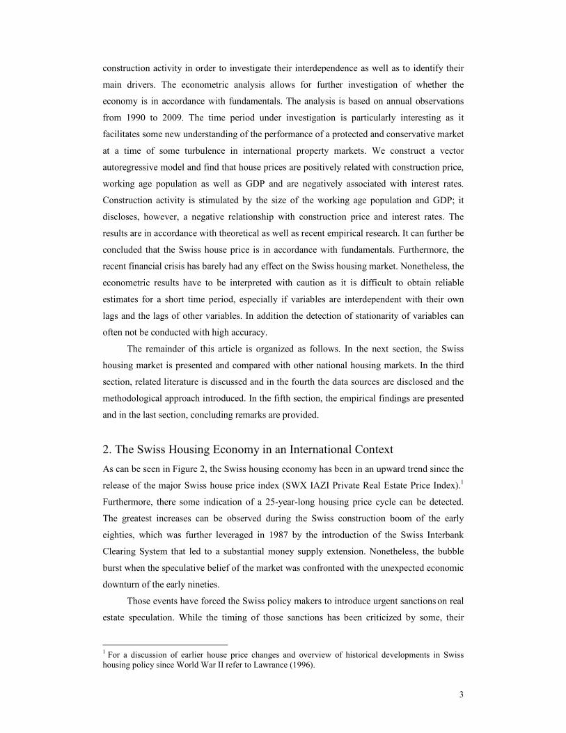
specification we depict in Figures 4 and 5 the estimated and actual house price and

construction activity developments, respectively. It is reassuring to observe that the model

tracks the actual changes in house prices and construction activity very closely.

6. Conclusion

In this research it is posited that a high degree of protectionism of a national housing

economy could lead to its stability. This study describes the unique features of the Swiss

housing economy and demonstrates efforts to compare it with other housing economies.

Furthermore, the determinants of house price and construction activity are modeled and the

associated dynamics are investigated. We cover a very interesting period of time, from 1990

to 2009, in which two substantial economic crises occurred. Focusing on this period allows

for an investigation of whether and how the Swiss housing market becomes affected by

economic turbulence. The drawback of the conducted econometric analysis is its short time

span and hence the results have to be interpreted with a word of caution.

We find that house prices are positively associated with construction prices, working

age population as well as GDP and are negatively associated with interest rates. Construction

activity is positively related to working age population and GDP and has a negative

relationship with construction costs and interest rates. Based on our model the predictions

correspond well with actual data and indicate that the model is well specified. The findings

are consistent with the dominant view in the literature that the housing market is not very

efficient. Lagged house price changes are able to predict future house price growth. Similarly,

12

We set the indicator function equal to one for the duration of the crisis of the early 1990s (i.e. 1990-

1994) and the recent global financial crisis (i.e. 2006-2009). The results are robust to numerous

alterations of those particular years.

13

past changes in construction activities contain information pertinent to current construction

activities.

While the study does not explicitly link the degree of protectionism with house price

stability, it provides some indication of the existence of a relationship between those two. The

Swiss housing price is in accordance with fundamentals and there is no sign of over-valuation.

The determinants of housing price and construction activity are consistent with theory and

previous empirical studies. There was also no decline in the value of the Swiss housing

market in recent years, whereas most housing economies experienced substantial drops. The

national average asking price for residential properties was down by 43 per cent in Ireland

from its unrivalled high of 2007, 20 per cent in the United Kingdom, 13 per cent in Spain and

experienced large decreases among most developed economies (Global Property Guide,

2011). Over a similar time period, the Swiss house price rose steadily by up to 5 per cent

annually.

The reasons for the observed stability of the Swiss housing economy can only be

speculated. It is possible that large immigration flows of the most recent years have, to some

extent, counteracted the negative spillover effects of the international financial turbulence.

Nonetheless, even if the growth of the working-age population of the last five years is

considered (equal to just above 1 per cent), in light of Degen and Fischer (2010) and also the

results presented in this research, the impact on house prices would be expected to be in the

region of around 3.7 to 8.4 per cent and could hardly prevent double digit house price drops

that have been internationally observed. Of greater importance perhaps are the existing

policies that protect the Swiss housing market from any greater turbulence. Heavily restricted

speculation, due to legislative as well as fiscal regulations, in combination with constraints

imposed on foreign acquisition might have been among the most important determinants of

the observed stability. In addition, de-incentivized home-ownership as well as substantial

supportive and protective policies for tenants have most likely prevented over-borrowing to

some extent and hence resulted in the financial stability of Swiss households relative to other

countries. Finally, the conservative lending practices of the Swiss banking sector have

presumably prevented the kind of over-consumption which has occurred in other countries.

Future research and country-specific case studies are required in order to investigate what

kinds of regulations would be particularly meaningful and beneficial to the stability of a

housing economy.

14

References

[1] M. Ball. Planning delay and the responsiveness of english housing supply. Urban Studies,

48(2):349–362, 2011.

[2] K. J. Borowiecki. The determinants of house prices and construction: An empirical investigation

of the swiss housing economy. International Real Estate Review, 12(3):193–220, 2009.

[3] S. Bourassa and M. Hoesli. Why do the swiss rent? The Journal of Real Estate Finance and

Economics, 40(3):286–309, 2010.

[4] S.C. Bourassa, M. Hoesli and D. Scognamiglio. Housing Finance, Prices and Tenure in

Switzerland. Swiss Finance Institute Research Paper Series, 09(16), 2009.

[5] K. E. Case and R. J. Shiller. The efficiency of the market for single-family homes. American

Economic Review, 79(1):125–37, 1989.

[6] J. Clemente, A. Montanes, and M. Reyes. Testing for a unit root in variables with a double

change in the mean. Economics Letters, 59:175-182, 1998.

[7] Credit Suisse. Der Schweizer Immobilienmarkt. Fakten Und Trends. Credit Suisse Economic

Research, Mat.-Nr. 1511451, 5, 2000.

[8] K. Degen and A. M. Fischer. Immigration and swiss house prices. CEPR Discussion Paper, 7583,

2010.

[9] P. Englund and Y. M. Ioannides. House price dynamics: An international empirical perspective.

Journal of Housing Economics, 6(2):119–136, 1997.

[10] E. L. Glaeser, J. Gyourko, and R. E. Saks. Why have housing prices gone up? The American

Economic Review, 95(2):329–333, 2005.

[11] Global Property Guide. http://www.globalpropertyguide.com/ (accessed September 2011), 2011.

[12] J. A. Kahn, What Drives Housing Prices? FRB of New York Staff Report, No. 34, 2008.

[13] J. A. Kahn, Productivity Swings and Housing Prices. Current Issues in Economics and Finance,

15(3):1-8, 2009.

[14] R. J. Lawrence. Switzerland. In Balchin, P. (Ed) Housing Policy in Europe, (London, Routledge)

pp36-50, 1996.

[15] E. Levin, A. Montagnoli, and R. E. Wright. Demographic change and the housing market:

Evidence from a comparison of Scotland and England. Urban Studies, 46(1):27–43, 2009.

[16] S. Malpezzi. A simple error correction model of house prices. Journal of Housing Economics,

8(1):27–62, 1999.

[17] G. Meen. The time-series behavior of house prices: A transatlantic divide? Journal of Housing

Economics, 11(1):1–23, 2002.

[18] R. Meese and N. Wallace. House price dynamics and market fundamentals: The parisian housing

market. Urban Studies, 40(5-6):1027–1045, 2003.

[19] E. Oikarinen. Studies on Housing Price Dynamics. Turku Working Paper Series, A-9, 2007.

[20] E. Oikarinen. Interaction between housing prices and household borrowing: The finnish case.

Journal of Banking & Finance, 33(4):747–756, 2009.

15

[21] J. M. Poterba. Tax subsidies to owner-occupied housing: An asset-market approach. The

Quarterly Journal of Economics, 99(4):729–52, 1984.

[22] J. M. Poterba. House price dynamics: The role of tax policy. Brookings Papers on Economic

Activity, 22(2):143–204, 1991.

[23] E. Werczberger. Home Ownership and Rent Control in Switzerland. Housing studies, 12(3):337-

353, 1997.

16

Tables

Table 1. Descriptive Statistics.

Obs Mean Std. Dev. Min Max

∆hp_c 20 -0.35% 3.34% -6.33% 8.29%

∆constr 20 1.19% 10.39% -15.74% 21.04%

∆cp_c 20 -0.47% 2.73% -7.73% 3.47%

rir 20 3.12% 1.39% 1.01% 5.72%

∆pop 20 0.77% 0.43% 0.04% 1.67%

∆gdp/W 20 -2.14% 1.84% -8.86% 0.58%

Note: Mean, Std. Dev., Min and Max values are in percentages.

Table 2. Stationarity Tests.

1 lag

2 lags

3 lags

ADF PP ADF PP ADF PP

∆hp_c -2.961 -13.146** -2.302 -12.891** -2.055 -12.403

∆constr -3.794*** -22.882*** -3.152** -21.738*** -2.317 -19.851***

∆cp_c -3.627** -14.622** -1.867 -12.282 -2.929 -11.197

Rir -0.749 -3.279 -0.343 -3.627 -0.911 -3.177

∆pop -2.124 -8.563 -2.039 -8.570 -1.948 -8.681

∆gdp/W -4.084*** -21.981*** -2.992** -19.903*** -2.396 -18.095***

∆unemp. -3.973*** -16.330** -2.581 -14.968** -2.833 -13.426**

Note: 'ADF' denotes the Augmented Dickey-Fuller test. 'PP' denotes the Phillips-Perron test. Standard

errors in parentheses. *** p<0.01, ** p<0.05.

17

Table 3. House Prices and Construction Activity.

(1) (2) (3) (4) (5) (6)

∆hp_ct ∆constrt ∆hp_ct ∆constrt ∆hp_ct ∆constrt

∆hp_ct-1 -0.0248 -1.532*** -0.0422 -1.502*** -0.0426 -1.502***

(0.112) (0.386) (0.105) (0.381) (0.0992) (0.381)

∆hp_ct-2 -1.048*** -0.318 -0.941*** -0.501 -0.920*** -0.499

(0.146) (0.502) (0.149) (0.540) (0.141) (0.543)

∆constrt-1 -0.0913** 0.420*** -0.0767 0.394*** -0.0691 0.395***

(0.0418) (0.144) (0.0398) (0.145) (0.0381) (0.146)

∆constrt-2 0.136*** -0.182 0.135*** -0.180 0.126*** -0.181

(0.0337) (0.116) (0.0314) (0.114) (0.0303) (0.116)

∆cp_ct 0.299*** -1.788*** 0.0925 -1.433** 0.146 -1.429**

(0.116) (0.398) (0.159) (0.579) (0.155) (0.594)

rirt-1 -0.0200*** -0.0604*** -0.0200*** -0.0604*** -0.0198*** -0.0604***

(0.00232) (0.00799) (0.00216) (0.00786) (0.00205) (0.00787)

∆popt 7.585*** 16.94*** 7.742*** 16.67*** 6.891*** 16.61***

(1.132) (3.899) (1.057) (3.847) (1.150) (4.415)

∆gdp/W, t 0.692*** 2.382*** 0.563*** 2.604*** 0.562*** 2.604***

(0.170) (0.586) (0.174) (0.635) (0.165) (0.635)

∆unemp t -0.00968 0.0166 -0.00908 0.0167

(0.00549) (0.0200) (0.00522) (0.0200)

crisis 0.00909 0.000673

(0.00603) (0.0232)

constant 0.0202** 0.107*** 0.0162* 0.114*** 0.0188** 0.114***

(0.00898) (0.0309) (0.00866) (0.0315) (0.00840) (0.0322)

R2 0.88 0.85 0.90 0.86 0.91 0.86

AIC -7.995 -7.995 -8.087 -8.087 -8.026 -8.026

HQIC -7.801 -7.801 -7.873 -7.873 -7.793 -7.793

SBIC -6.999 -6.999 -6.991 -6.991 -6.831 -6.831

Observation 20 20 20 20 20 20

Note: Standard errors in parentheses. All specifications contain controls for the years 1994 and 2005

at which a structural break in the house price series occurred. The Crisis dummy takes the value one

for the years 1990 to 1994 and 2006 to 2009, and zero otherwise. Description of remaining variables

is presented in Table A1 in the Appendix. *** p<0.01, ** p<0.05.

18

Figures

Figure 1. Property Price Index and House Price Changes.

AT

BE

BU

CZ

DE

FR

GR

HU

IC

IT

LI

MA

NL

NO

RU

SR

ESSE

CH

UA

GB

0100

200

300

400

500

House Price Changes, 10 Years (%)

20 40 60 80 100Property Rights Index

Source: Property Rights Index and House Price Changes are obtained from Global Property Guide (2011), for

Austria (AT), Belgium (BE), Bulgaria (BU), Czech Republic (CZ), Germany (DE), France (FR), Greece (GR),

Hungary (HU), Iceland (IC), Italy (IT), Lithuania (LI), Malta (MA), Netherlands (NL), Norway (NO), Russia (RU), Serbia (SR), Spain (ES), Sweden (SE), Switzerland (CH), Ukraine (UA) and United Kingdom (GB).

19

Figure 2. Swiss house price 1982 to 2010.

60

80

100

120

140

House Price Index

1980 1990 2000 2010Year

Source: SWX IAZI Private Real Estate Price Index.

20

Figure 3. Risk-return profiles of international housing economies.

Source: Borowiecki (2009). Note: Switzerland (CH) is based on the inflation adjusted SWX IAZI Private Real

Estate Price Index. BIS calculation based on national data is employed for all remaining countries, that is Australia

(AU), Belgium (BE), Canada (CA), Denmark (DK), Finland (FI), France (FR), Germany (DE), Ireland (IE), Italy

(IT), Japan (JP), Netherlands (NL), New Zealand (NZ), Norway (NO), Spain (ES), Sweden (SE), Switzerland

(CH), United Kingdom (GB) and United States (US)). The covered time period is 1981 to 2006.

21

Figure 4. Predicted and actual house price growth.

-.1

-.05

0.05

.1

1990 1995 2000 2005 2010Year

Predicted D.HP Actual D.HP

Note: Predicted house price growth is based on the specification presented in column (1), Table 3.

22

Figure 5. Predicted and actual construction activity growth.

-.2

-.1

0.1

.2

1990 1995 2000 2005 2010Year

Predicted D.CONS Actual D.CONS

Note: Predicted construction activity growth is based on the specification presented in column (2), Table 3.

23

Ap

pen

dix

Appen

dix

1. D

ata

sou

rces

and v

aria

ble

des

crip

tion.

V

aria

ble

nam

e S

ourc

e V

aria

ble

des

crip

tion

∆hp

_c

SW

X I

AZ

I P

rivat

e

Rea

l E

stat

e P

rice

Index

1982-2

010

SW

ISS

EX

CH

AN

GE

Th

is i

ndex

is

a w

eigh

ted a

ggre

gat

e of

the

SW

X I

AZ

I P

rivat

e H

ou

se P

rice

Ind

ex a

nd

SW

X I

AZ

I C

on

dom

iniu

m P

rice

Ind

ex.

It i

s ca

lcula

ted

bas

ed o

n a

nonym

ou

s tr

ansa

ctio

n

dat

a p

rovid

ed b

y b

ank

s, i

nsu

rers

and p

ensi

on

funds.

CP

I ad

just

ed,

log c

han

ge

from

pre

vio

us

yea

r.

∆co

nst

r H

ousi

ng c

on

stru

ctio

n

1981-2

009

SN

B

Num

ber

of

apar

tmen

ts u

nd

er c

onst

ruct

ion, lo

g c

han

ge

from

pre

vio

us

yea

r.

∆cp

_c

Const

ruct

ion P

rice

Index

1989-2

009

SN

B

Th

is c

onst

ruct

ion c

ost

index

cover

s re

sid

enti

al p

rop

erti

es (

house

s an

d c

ondo

min

ium

s).

CP

I ad

just

ed, lo

g c

han

ge

from

pre

vio

us

yea

r.

rir

Rea

l in

tere

st r

ate

1989-2

009

SN

B

Dis

count

rate

(‘S

pec

ial

rate

bo

ttle

nec

k f

inan

cing f

acil

ity’)

. A

dju

sted

by t

he

con

sum

er

pri

ce i

nfl

atio

n r

ate.

∆po

p

Pop

ula

tion

1980-2

009

SN

B

Work

ing a

ge

pop

ula

tion (

aged

20 t

o 6

4).

Lo

g c

han

ge

from

pre

vio

us

yea

r.

∆gd

p/W

GD

P

1980-2

009

IMF

C

han

ge

in S

wis

s G

DP

rel

ativ

e to

worl

d G

DP

. C

PI

adju

sted

.

∆un

emp

Un

emplo

ym

ent

1980-2

009

IMF

C

han

ge

in S

wis

s U

nem

plo

ym

ent

CP

I

Consu

mer

Pri

ce I

ndex

1980-2

010

IMF

S

wis

s co

nsu

mer

pri

ce i

ndex

.

24

Appen

dix

2. In

novat

ional

outl

ier

unit

roo

t te

st.

1.11.21.31.41.5hp_all_cpi

1990

1995

2000

2005

2010

year

Test on hp_all_cpi: breaks at 1994,2005

-.1-.050.05.1D.hp_all_cpi

1990

1995

2000

2005

2010

year

D.hp_all_cpi

Clemente-Montañés-Reyes double IO test for unit root