DYNAMICS BETWEEN MALAYSIAN EQUITY MARKET AND...
49
DYNAMICS BETWEEN MALAYSIAN EQUITY MARKET AND MACROECONOMIC VARIABLES: AN APPLICATION OF KALMAN FILTER MODEL WITH HETEROSKEDASTIC ERROR by CHEAH LEE HEN Thesis submitted in fulfilment of the requirements for the degree of Master of Science in Statistics DECEMBER 2006
Transcript of DYNAMICS BETWEEN MALAYSIAN EQUITY MARKET AND...
DYNAMICS BETWEEN MALAYSIAN EQUITY MARKET AND MACROECONOMIC VARIABLES: AN APPLICATION OF KALMAN FILTER
MODEL WITH HETEROSKEDASTIC ERROR
by
CHEAH LEE HEN
Thesis submitted in fulfilment of the requirements for the degree
of Master of Science in Statistics
DECEMBER 2006

ACKNOWLEDGEMENTS
First of all I would like to thank my supervisor, Dr. Zainudin Arsad, for his
overwhelmingly help and support over the past two years of my research. This thesis
would not have been possible without him, and I am extremely grateful for his
encouragement and patience through very difficult time.
I wish to thank the Dean of School of Mathematical Sciences, Associate
Professor Dr. Ahmad Izani bin Md. Ismail for his assistance during my studies
especially in financing me to attend conferences and symposiums. I am also grateful to
all the staffs in School of Mathematical Sciences for their continuing aid in completing
my thesis. My appreciation also goes to the Perpustakaan Hamzah Sendut Universiti
Sains Malaysia for various obtainable materials.
Last but not least, I would like to thank my parents, Cheah Back Liang and Lim
Lang Hiang, sisters, brothers, a true friend and all of whom expressed a continual faith
in me, for their unbounded encouragement, support and patience. I truly appreciate
their kindness for being there when I needed them. Thanks should also go to past and
present fellow research students in Makmal Siswazah II for a friendly environment.
ii

TABLE OF CONTENTS
Page ACKNOWLEDGEMENTS ii
TABLE OF CONTENTS iii
LIST OF TABLES viii
LIST OF FIGURES xi
LIST OF APPENDICES xviii
LIST OF PUBLICATIONS xviii
ABSTRAK xix
ABSTRACT xxii CHAPTER 1 INTRODUCTION
1.1 Overviews of the Malaysian economy 1
1.2 Bursa Malaysia 2
1.3 Literature review 6
1.3.1 Relationship between stock prices and stock index futures prices
6
1.3.2 Relationship between stock prices and foreign exchange rates
12
1.3.3 Application of Kalman filter technique (KF) and Generalized Autoregressive Conditional Heteroskedaticity (GARCH)
19
1.4 Objectives 31
1.5 Data 33
CHAPTER 2 METHODOLOGY 2.1 Introduction 34
2.2 Data analysis 34
2.3 Box & Jenkins ARIMA model 36
2.3.1 Model specification 39
2.3.2 Estimation of the ARMA model 42
2.3.3 Diagnostic checking 43
2.3.4 Forecasting 44
2.4 Model selection criteria 47
2.5 The state-space form representation of a linear dynamic system 48
2.6 The Kalman filter technique 51
2.6.1 Start of the recursion and initial conditions 51
iii

2.6.2 Prediction 54
2.6.3 Prediction of observed vector 54
2.6.4 Updating 55
2.6.5 Forecasting with the Kalman filter 56
2.6.6 Maximum likelihood estimation of parameters 58
2.7 Conditional heteroskedasticity modeling 59
2.7.1 Introduction 59
2.7.2 ARCH 61
2.7.3 GARCH 62
2.7.4 ARCH-M 63
2.7.5 TARCH 63
2.7.6 EGARCH 64
2.7.7 Estimation and diagnostic test of GARCH model 65
2.8 State-space model with ARCH disturbances 66
2.9 Vector Autoregression (VAR) 69
2.10 Unit Root Test 71
CHAPTER 3 THE KALMAN FILTER MODEL FOR STOCK PRICES 3.1 Introduction 74
3.2 Descriptive statistics 75
3.2.1 Kuala Lumpur Composite Index (KLCI) 75
3.2.2 Kuala Lumpur Composite Index Futures (FKLI) 81
3.2.3 Pound Sterling (STL) 87
3.3 Unit Root Test 91
3.4 Kalman filter AR(1) and ARMA(1,0) 93
3.5 Motivation for the subsequent analyses: The Wilkie inflation model 96
3.6 Kalman filter model, 0C = 99
3.7 Kalman filter model, 0C ≠ 102
3.8 Allowing noises to be correlated, 12 0S ≠ 104
3.9 Allowing to be estimated μ 108
3.10 Analysis of the residuals 109
3.11 Judging the performance between models: Within-sample and out-
of-sample long-term forecast error
112
3.12 Simulation study of Kalman filter models 117
3.13 Maximisation problem 119
iv
CHAPTER 4 KALMAN FILTER MODEL WITH HETEROSKEDASTIC DISTURBANCES FOR STOCK PRICES
4.1 Background of ARCH model 121
4.2 Model specification: State-space model with heteroskedastic
disturbances
124
4.3 Simple ARCH-type models 127
4.4 Kalman filter-ARCH-type combination models 129
4.4.1 Kalman filter-ARCH(1) model 129
4.4.2 Kalman filter-GARCH(1,1) model 131
4.4.3 Kalman filter-GARCH(1,1)-M model 131
4.4.4 Kalman filter-EGARCH(1,1) model 132
4.4.5 Kalman filter-TARCH(1,1) model 133
4.5 Comparisons among the Kalman filter-ARCH-type combination
models
134
4.6 Allowing noises to be correlated, 12 0S ≠ 142
4.7 Comparison of pure Kalman filter and Kalman filter-ARCH-type
combination models
151
4.8 Comparison of pure ARCH-type models and Kalman filter-ARCH-
type combination models
153
4.9 Analysis of the residuals 155
4.10 Judging performance between models: Within-sample and out-of-
sample long-term forecast error
159
4.11 Simulation study of Kalman filter-ARCH-type models 162
CHAPTER 5 A MODEL FOR STOCK PRICES, EXCHANGE RATES
AND FINANCIAL FUTURES 5.1 Introduction 165
5.2 VAR model for stock prices, exchange rates and financial futures 166
5.3 The Kalman filter model for stock prices, exchange rates and
financial futures
170
5.3.1 Relationship between stock prices and exchange rates 171
5.3.2 Relationship between stock prices and financial futures 173
5.3.3 Relationship between stock prices, exchange rates and financial futures
173
5.3.4 The Kalman filter: Restructuring with the addition of an unobserved series
179
v
5.4 The Kalman filter-ARCH-type models for stock prices, exchange
rates and financial futures
185
5.4.1 Relationship between stock prices and exchange rates 186
5.4.2 Relationship between stock prices and financial futures 189
5.4.3 Relationship between stock prices, exchange rates and financial futures
192
5.4.4 The Kalman filter-EGARCH model: Restructuring with the addition of an unobserved series
200
5.5 Analysis of the residuals 204
5.5.1 Restructuring of the model 206
5.6 Judging performance between models: Within-sample and out-of-
sample long-term forecast error
210
5.7 Simulation study of Kalman filter and Kalman filter-EGARCH
models
215
CHAPTER 6 INTERACTION AMONG STOCK PRICES, EXCHANGE
RATES AND FINANCIAL FUTURES 6.1 Introduction 219
6.2 The Kalman filter with zero measurement error 219
6.3 The Kalman filter-EGARCH model 228
6.4 Residual analysis 233
6.4.1 Restructuring of the model 234
6.5 Judging the performance: Within-sample and out- of-sample long-
term forecast error
237
6.6 Simulation study for the daily data 240
CHAPTER 7 CONCLUSIONS AND FUTURE RESEARCH 7.1 Discussions 249
7.2 Suggestions for future research 253
BIBLIOGRAPHY
255
APPENDICES
Appendix 1 Abstracts of conference papers
Appendix 2 Full paper awarded Best Paper at MFA and submitted to CMR
vi

Appendix 3 Data
Appendix 4 S-Plus programming scripts
vii
LIST OF TABLES
Page
2.1 Theoretical patterns of ACF and PACF 41
3.1 Descriptive statistics for KLCI returns for daily data 76
.3.2 Descriptive statistics of KLCI returns for monthly data 79
3.3 Descriptive statistics of FKLI returns for daily data 82
3.4 Descriptive statistics of FKLI returns for monthly data 86
3.5 Descriptive statistics of Pound Sterling returns for daily data 88
3.6 3.7 3.8
Descriptive statistics of Pound Sterling returns for monthly data Unit-root testing results (original) Unit-root testing results (returns)
89
92
92
3.9 Estimated parameters for the Box & Jenkins and the Kalman filter model
94
3.10 Estimated parameters and standard error of Kalman filter model 0C =
100
3.11 Estimated parameters and standard error of Kalman filter model 0C ≠
103
3.12 Estimated parameters and standard error of Kalman 0C = and with 0C ≠ 12 0S ≠
105
3.13 Estimated parameters and standard error of Kalman 0C = and with 0C ≠ 0μ ≠
109
3.14 Comparison of residuals from various models using basic statistics
111
3.15 LM test for residuals-squared from various models 112
3.16 Out-of-sample prediction errors from various models 114
4.1 Comparisons of statistical goodness of fit for various ARCH-type models
128
4.2 Estimated parameters for various ARCH-type models 128
4.3 Estimated parameters for Kalman filter-ARCH-type combination models
130
4.4 Estimated parameter for Kalman filter-ARCH-type combination models, 12 0S ≠
143
4.5 Comparisons of statistical goodness of fit for various Kalman filter-ARCH-type combination models
151
4.6 Within-sample and out-of-sample forecast error for pure Kalman filter and various Kalman filter-ARCH-type models
152
viii
4.7 Comparisons of statistical goodness of fit for Kalman filter-ARCH-type combination models with the corresponding pure ARCH-type models
154
4.8 Comparison residuals of various models using basic statistics 156
4.9 LM test for residuals-squared from various models 158
4.10 Out-of-sample forecast error for different models 162
5.1 Estimate of Vector Autoregressive model for KLCI and FKLI 167
5.2 Estimate of Vector Autoregressive model for KLCI and STL 167
5.3 Estimate of Vector Autoregressive model for KLCI, STL and FKLI 168
5.4 Dynamics between KLCI with STL and FKLI respectively from Kalman filter
172
5.5 Dynamics between KLCI, STL and FKLI from Kalman filter 175
5.6 Dynamics between KLCI, FKLI, STL and an unobserved series from Kalman filter
181
5.7 Dynamics between KLCI and STL for Kalman filter-ARCH-type models
188
5.8 Dynamics between KLCI and FKLI for Kalman filter-ARCH-type models
190
5.9(a) Dynamics between KLCI, STL and FKLI for Kalman filter-ARCH-type models
193
5.9(b) Dynamics between KLCI, STL and FKLI for Kalman filter-ARCH-type models: Variance equation
194
5.10 Dynamics between KLCI, STL, FKLI and unobserved series from KF-EGARCH
201
5.11 Basic statistics of residuals from different models 206
5.12 Dynamics between KLCI, STL and FKLI from KF-restructured model
210
5.13(a) Within sample one-step-ahead prediction error, 11 2| 1t tP C− + for
pure KF and KF-ARCH-type models
211
5.13(b) Out-of-sample one-step-ahead prediction error for pure KF and KF-ARCH-type models
212
5.13(c) Out-of-sample long-term 100-steps-ahead forecast error for pure KF and KF-ARCH-type models
212
5.14(a) Within-sample one-step-ahead prediction error for the restructured model
214
5.14(b) Out-of-sample one-step-ahead prediction error for the restructured model
214
5.14(c) Out-of-sample long-term 100-steps-ahead forecast error for the restructured model
214
ix
6.1 Dynamics between KLCI, STL, FKLI and unobserved series: KF model
220
6.2 Dynamics between KLCI, STL, FKLI and an unobserved series: KF-EGARCH model
229
6.3 Basic statistics for residual from pure KF model 233
6.4 Basic statistics for residual from KF-EGARCH model 234
6.5 Dynamics between KLCI, STL, FKLI and unobserved series: KF-restructured model
237
6.6(a) Within-sample one-step-ahead prediction error from pure KF model
238
6.6(b) Within-sample one-step-ahead prediction error from KF-EGARCH model
238
6.7(a) Out-of-sample one-step-ahead prediction error from pure KF model
239
6.7(b) Out-of-sample one-step-ahead prediction error from KF-EGARCH model
240
6.8(a) Out-of-sample long-term 100-steps-ahead forecast error from pure KF model
240
6.8(b) Out-of-sample long-term 100-steps-ahead forecast error from KF-EGARCH model
240
x
LIST OF FIGURES
Page
1.1 The regulatory structure diagram (Reproduced from Bursa Malaysia)
4
1.2 Derivatives market structure in Malaysia (Reproduced from Bursa Malaysia)
5
2.1 Box-Jenkins modeling steps 40
3.1 Time series plot for daily price of KLCI 77
3.2 Time series plot for daily returns of KLCI 78
3.3 Histogram and normal curve for daily KLCI returns 78
3.4 Time series plot for monthly price of KLCI 80
3.5 Time series plot for monthly returns of KLCI 81
3.6 Time series plot for daily price of FKLI 84
3.7 Time series plot for daily returns of FKLI 85
3.8 Histogram and normal curve for daily FKLI returns 85
3.9 Time series plot for monthly price of FKLI 86
3.10 Time series plot for monthly returns of FKLI 86
3.11 Time series plot for daily price of Pound Sterling 89
3.12 Time series plot for daily returns of Pound Sterling 89
3.13 Histogram and normal curve for daily Pound Sterling returns 90
3.14 Time series plot for monthly price of Pound Sterling 90
3.15 Time series plot for monthly returns of Pound Sterling 91
3.16(a) KLCI returns and one-step-ahead estimates from Kalman filter AR(1) model
94
3.16(b) Magnified version of Figure 3.16(a) 95
3.17(a) KLCI returns and one-step-ahead estimates from B&J AR(1) model
95
3.17(b) Magnified version of Figure 3.17(a) 95
3.18(a) KLCI returns and one-step-ahead estimates of KLCI: Kalman filter 0C =
100
3.18(b) Mean reversionary level and one-step-ahead estimates of KLCI: Kalman filter model 0C =
101
3.19(a) KLCI returns and one-step-ahead estimates of KLCI: Kalman filter 0C ≠
104
xi
3.19(b) Mean reversionary level and one-step-ahead estimates of KLCI: Kalman filter 0C ≠
104
3.20(a) KLCI returns and one-step-ahead estimates of KLCI: Kalman filter , 0C = 12 0S ≠
106
3.20(b) Mean reversionary level and one-step-ahead estimates of KLCI: Kalman filter , 0C = 12 0S ≠
107
3.21(a) KLCI returns and one-step-ahead estimates of KLCI: Kalman filter , 0C ≠ 12 0S ≠
107
3.21(b) Mean reversionary level and one-step-ahead estimates of KLCI: Kalman filter , 0C ≠ 12 0S ≠
107
3.22(a) Autocorrelation function of squared-residuals: Kalman filter 0C = 110
3.22(b) Partial autocorrelation function of squared-residuals: Kalman filter 0C =
110
3.23(a) Autocorrelation function of squared-residuals: Kalman filter 0C ≠ 110
3.23(b) Partial autocorrelation function of squared-residuals: Kalman filter 0C ≠
111
3.24 Within-sample one-step-ahead estimates of prediction error 113
3.25(a) Out-of-sample one-step-ahead forecasts from the proposed models
116
3.25(b) Magnified version of Figure 3.25(a) 117
3.26 Out-of-sample multi-steps forecasts from the proposed models 117
3.27 Five simulated KLCI series using the Kalman filter 0C = , model. Also shown are KLCI returns (bold series) and
the 5%, 25%, 75% and 95% quantiles 12 0S ≠
118
3.28 Five simulated KLCI series using the Kalman filter 0C ≠ , model. Also shown are KLCI returns (bold series) and
the 5%, 25%, 75% and 95% quantiles 12 0S =
119
4.1(a) KLCI returns and one-step-ahead estimates of KLCI from KF-ARCH model
136
4.1(b) One-step-ahead estimates of KLCI from KF-ARCH model 136
4.1(c) Mean reversionary level of KLCI from KF-ARCH model 137
4.2(a) KLCI returns and one-step-ahead estimates of KLCI from KF-GARCH model
137
4.2(b) One-step-ahead estimates of KLCI from KF-GARCH model 137
4.2(c) Mean reversionary level of KLCI from KF-GARCH model 138
4.3(a) KLCI returns and one-step-ahead estimates of KLCI from KF-GARCH-M model
138
4.3(b) One-step-ahead estimates of KLCI from KF-GARCH-M model 138
4.3(c) Mean reversionary level of KLCI from KF-GARCH-M model 139
xii
4.4(a) KLCI returns and one-step-ahead estimates of KLCI from KF-EGARCH model
139
4.4(b) One-step-ahead estimates of KLCI from KF-EGARCH model 139
4.4(c) Mean reversionary level of KLCI from KF-EGARCH model 140
4.5(a) KLCI returns and one-step-ahead estimates of KLCI from KF-TARCH model
140
4.5(b) One-step-ahead estimates of KLCI from KF-TARCH model 140
4.5(c) Mean reversionary level of KLCI from KF-TARCH model 141
4.6(a) KLCI returns and estimate of confidence interval (dotted line) from KF, KF-ARCH and KF-GARCH models
141
4.6(b) KLCI returns and estimate of confidence interval from KF, KF-GARCH-M and KF-EARCH models
141
4.6(c) KLCI returns and estimate of confidence interval from KF-TARCH model
142
4.7(a) One-step-ahead estimates of KLCI from KF-GARCH model 12 0S ≠
146
4.7(b) Mean reversionary level of KLCI from KF-GARCH 12 0S ≠ model 146
4.7(c) Comparisons of one-step-ahead estimates of KLCI from KF-GARCH (solid line) and 12 0S = 12 0S ≠ (dotted line)
147
4.7(d) Comparisons of mean reversionary level of KLCI from KF-GARCH (solid line) and 12 0S = 12 0S ≠ (dotted line)
147
4.8(a) One-step-ahead estimates of KLCI from KF-EGARCH model 12 0S ≠
147
4.8(b) Mean reversionary level of KLCI from KF-EGARCH model 12 0S ≠
148
4.8(c) Comparisons of one-step-ahead estimates of KLCI from KF-EGARCH (solid line) and 12 0S = 12 0S ≠ (dotted line)
148
4.8(d) Comparisons of mean reversionary level of KLCI from KF-EGARCH (solid line) and 12 0S = 12 0S ≠ (dotted line)
148
4.9(a) One-step-ahead estimates of KLCI from KF-TARCH model 12 0S ≠
149
4.9(b) Mean reversionary level of KLCI from KF-TARCH 12 0S ≠ model 149
4.9(c) Comparisons of one-step-ahead estimates of KLCI from KF-TARCH (solid line) and 12 0S = 12 0S ≠ (dotted line)
149
4.9(d) Comparisons of mean reversionary level of KLCI from KF-TARCH (solid line) and 12 0S = 12 0S ≠ (dotted line)
150
4.10 Autocorrelation function of squared-residual from Kalman filter-GARCH-M model 12 0S =
156
4.11 Partial autocorrelation function of squared-residual from Kalman filter-GARCH-M 12 0S = model
157
xiii

4.12 Autocorrelation function of squared-residual from Kalman filter-GARCH model 12 0S ≠
157
4.13 Partital autocorrelation function of squared-residual from Kalman filter-GARCH model 12 0S ≠
157
4.14 Within-sample prediction error, 1| −ttP from various models 160
4.15 Out-of-sample one-step-ahead forecasts from various models 160
4.16 Out-of-sample long-term (100-months) forecasts from various models
161
4.17 Five simulated KLCI series using the Kalman filter-GARCH-M 12 0S = model. Also shown are KLCI returns (in bold) with the 5%, 25%, 75% and 95% quantiles
163
4.18 Five simulated KLCI series using the Kalman filter-GARCH model. Also shown are KLCI returns (in bold) with the
5%, 25%, 75% and 95% quantiles 12 0S ≠
163
5.1(a) KLCI returns and one-step-ahead estimates from Kalman filter 0C =
177
5.1(b) STL returns and one-step-ahead estimates from Kalman filter 0C =
177
5.1(c) FKLI returns and one-step-ahead estimates from Kalman filter 0C =
177
5.2(a) Comparison of one-step-ahead estimates of the KLCI series: KF (solid line), KF 0C = 0C ≠ (dotted line)
178
5.2(b) Comparison of one-step-ahead estimates of the STL series: KF (solid line), KF 0C = 0C ≠ (dotted line)
178
5.2(c) Comparisons of one-step-ahead estimates of the FKLI series: KF 0C = (solid line), KF 0C ≠ (dotted line)
178
5.3(a) KLCI returns and one-step-ahead estimates for KF-U model 183
5.3(b) STL returns and one-step-ahead estimates for KF-U model 183
5.3(c) FKLI returns and one-step-ahead estimates for KF-U model 183
5.4(a) KLCI returns and unobserved series for KF-U model 184
5.4(b) STL returns and unobserved series for KF-U model 184
5.4(c) FKLI returns and unobserved series for KF-U model 184
5.5 Relationship and direction of effect between KLCI, STL and FKLI series for Kalman filter-ARCH-type models
197
5.6(a) KLCI returns and one-step-ahead estimates for KF-EGARCH model
198
5.6(b) STL returns and one-step-ahead estimates for KF-EGARCH model
198
5.6(c) FKLI returns and one-step-ahead estimates for KF-EGARCH model
198
xiv
5.7(a) Comparison of one-step-ahead estimates of the KLCI series: KF (dotted line), KF-EGARCH (solid line) 0C =
199
5.7(b) Comparison of one-step-ahead estimates of the STL series: KF (dotted line), KF-EGARCH (solid line) 0C =
199
5.7(c) Comparison of one-step-ahead estimates of the FKLI series: KF (dotted line), KF-EGARCH (solid line) 0C =
199
5.8(a) KLCI returns and unobserved series for KF-EGARCH-U model 203
5.8(b) STL returns and unobserved series for KF-EGARCH-U model 203
5.8(c) FKLI returns and unobserved series for KF-EGARCH-U model 203
5.9 Correlation between residuals, KLCI and STL: KF 0C = (Correlation=-0.202)
207
5.10 Correlation between residuals, KLCI and FKLI: KF 0C = (Correlation0.999)
207
5.11 Correlation between residuals, KLCI and STL: KF-restructured (Correlation=-0.200)
208
5.12 Correlation between residuals, KLCI and FKLI: KF-restructured (Correlation=0.359)
208
5.13(a) Five simulated KLCI series using the Kalman filter model. Also shown are KLCI returns (bold series) and the 5%, 25%, 75% and 95% quantiles
216
5.13(b) Five simulated STL series using the Kalman filter model. Also shown are STL returns (bold series) and the 5%, 25%, 75% and 95% quantiles
216
5.13(c) Five simulated FKLI series using the Kalman filter model. Also shown are FKLI returns (bold series) and the 5%, 25%, 75% and 95% quantiles
217
5.14(a) Five simulated KLCI series using the Kalman filter-EGARCH model. Also shown are KLCI returns (bold series) and the 5%, 25%, 75% and 95% quantiles
217
5.14(b) Five simulated STL series using the Kalman filter-EGARCH model. Also shown are STL returns (bold series) and the 5%, 25%, 75% and 95% quantiles
218
5.14(c) Five simulated FKLI series using the Kalman filter-EGARCH model. Also shown are FKLI returns (bold series) and the 5%, 25%, 75% and 95% quantiles
218
6.1 Relationship and direction of effect between KLCI, STL and FKLI from Kalman filter model during World Recession and Recovery periods
222
6.2 Returns series (solid line) and one-step-ahead estimates (dotted line): World Recession period. KLCI (top), STL (middle), FKLI (bottom)
224
xv
6.3 Returns series (solid line) and one-step-ahead estimates (dotted line): First Recovery period. KLCI (top), STL (middle), FKLI (bottom)
225
6.4 Returns series (solid line) and one-step-ahead estimates (dotted line): Second Recovery period. KLCI (top), STL (middle), FKLI (bottom)
226
6.5 Comparisons of unobserved series and KLCI returns (top), STL returns (middle), FKLI returns (bottom) from KF model: Second Recovery period
227
6.6 Relationship and direction of effect between KLCI, STL and FKLI from Kalman filter-EGARCH model during World Recession and Recovery periods
231
6.7 Comparisons of unobserved series for KF and KF-EGARCH models: World Recession period (top), First Recovery period (middle), Second Recovery period (bottom)
232
6.8 Correlation between residuals, KLCI and STL: KF, 2nd Recovery period (Correlation=0.031)
234
6.9 Correlation between residuals, KLCI and FKLI: KF, 2nd Recovery period (Correlation=0.817)
235
6.10 Correlation between residuals, KLCI and STL: KF-restructured, 2nd Recovery period (Correlation=0.001)
235
6.11 Correlation between residuals, KLCI and FKLI: KF-restructured, 2nd Recovery period (Correlation=0.006)
235
6.12(a) Five simulated KLCI series using the Kalman filter model. Also shown are KLCI returns (in bold) and the 5%, 25%, 75% and 95% quantiles (Oct 2003 to May 2004)
242
6.12(b) Five simulated KLCI series using the Kalman filter model. Also shown are KLCI returns (in bold) with the 5%, 25%, 75% and 95% quantiles (June 2004 to Jan 2005)
242
6.13(a) Five simulated STL series using the Kalman filter model. Also shown are STL returns (in bold) with the 5%, 25%, 75% and 95% quantiles (Oct 2003 to May 2004)
243
6.13(b) Five simulated STL series using the Kalman filter model. Also shown are STL returns (in bold) with the 5%, 25%, 75% and 95% quantiles (June 2004 to Jan 2005)
243
6.14(a) Five simulated FKLI series using the Kalman filter model. Also shown are FKLI returns (in bold) and the 5%, 25%, 75% and 95% quantiles (Oct 2003 to May 2004)
244
6.14(b) Five simulated FKLI series using the Kalman filter model. Also shown are FKLI returns (in bold) with the 5%, 25%, 75% and 95% quantiles (June 2004 to Jan 2005)
244
6.15(a) Five simulated KLCI series using the Kalman filter-EGARCH model. Also shown are KLCI returns (in bold) with the 5%, 25%, 75% and 95% quantiles (Oct 2003 to May 2004)
245
xvi
6.15(b) Five simulated KLCI series using the Kalman filter model. Also shown are KLCI returns (in bold) with the 5%, 25%, 75% and 95% quantiles (June 2004 to Jan 2005)
245
6.16(a) Five simulated STL series using the Kalman filter-EGARCH model. Also shown are STL returns (in bold) with the 5%, 25%, 75% and 95% quantiles (Oct 2003 to May 2004)
246
6.16(b) Five simulated STL series using the Kalman filter EGARCH model. Also shown are STL returns (in bold) with the 5%, 25%, 75% and 95% quantiles (June 2004 to Jan 2005)
246
6.17(a) Five simulated FKLI series using the Kalman filter-EGARCH model. Also shown are FKLI returns (in bold) with the 5%, 25%, 75% and 95% quantiles (Oct 2003 to May 2004)
247
6.17(b) Five simulated FKLI series using the Kalman filter- EGARCH model. Also shown are FKLI returns (in bold) with the 5%, 25%, 75% and 95% quantiles (June 2004 to Jan 2005)
247
xvii

LIST OF APPENDICES
1.1 Investigation on the Malaysian equity market using state-space
formulation: A comparison to the ARMA model
1.2 Application of Kalman filter and its extensions to model the Composite Index return at Bursa Malaysia
1.3 Causal relationships between stock prices and macroeconomic variables in Malaysia
1.4 World crisis for Malaysian equity market: State-space model
1.5 Estimating and forecasting volatility of Malaysian stock market using a combination of Kalman filter and GARCH models
1.6 Dynamics between the Malaysian equity market and macroeconomic variables: A comparison of Kalman filter and GARCH model
1.7 Application of Kalman filter technique and Vector Autoregressive to investigate the dynamics between the equity markets
2.1 Estimating and forecasting volatility of Malaysian stock market using a combination of Kalman filter and GARCH models
3.1 Monthly data of Kuala Lumpur Composite Index (KLCI)
3.2 Monthly data of Kuala Lumpur Composite Index Futures (FKLI) and Pound Sterling (STL)
3.3 Daily data of Kuala Lumpur Composite Index (KLCI), Pound Sterling (STL) and Kuala Lumpur Composite Index Futures (FKLI)
4.1 Kalman filter model
4.2 Kalman filter-GARCH model
4.3 Standard error of parameters
LIST OF PUBLICATIONS
1 CHeah, L. H. and Arsad, Z. (2006). Estimating And Forecasting
Volatility Of Malaysian Stock Market Using A Combination Of Kalman Filter And GARCH Models. Capital Market Reviews, 14, (1 & 2), 27-42.
xviii
DINAMIK ANTARA PASARAN EKUITI MALAYSIA DAN PEMBOLEHUBAH-PEMBOLEHUBAH MAKROEKONOMI: SATU APLIKASI
MODEL PENAPIS KALMAN DENGAN RALAT HETEROSKEDASTIK
ABSTRAK
Sejak diperkenalkan oleh Kalman dan Bucy (1960), model penapis Kalman
telah mendapat penggunaan yang luas dalam dalam program ruang angkasa dan
bidang kejuteraan kawalan. Namun begitu, pengaplikasiannya dalam bidang siri masa
kewangan masih jarang digunakan dan jauh ketinggalan. Model penapis Kalman
adalah satu set persamaan yang membenarkan nilai anggaran dikemaskini sebaik
sahaja satu cerapan baru diperolehi. Satu model untuk data bulanan Indeks Komposit
Kuala Lumpur dari April 1986 hingga Februari 2005 dicadang dan dikaji. Model ini
membenarkan aras berbalik purata bagi Index Komposit Kuala Lumpur dimodelkan
secara stokastik. Perbandingan dilakukan menggunakan keputusan-keputusan di
antara model ringkas penapis Kalman AR(1) dan penapis Kalman tulen yang dicadang.
Model terbaik dipilih berdasarkan nilai log kebolehjadian maksimum, Akaike
Information Criterion dan Bayesian Information Criterion.
Tesis ini juga menggunakan model penapis Kalman untuk menganalisa ruang
keadaan dengan ralat bersifat ARCH seperti yang dicadangkan oleh Harvey, Ruiz and
Sentana (1992). Analisis difokuskan terhadap model-model yang mana sebutan-
sebutan ralat dalam persamaan pengukuran adalah heteroskedastik. Lima model dari
jenis ARCH termasuk ARCH, GARCH, GARCH-M, EGARCH dan TARCH
dipertimbangkan. Keputusan menunjukkan bahawa model-model dengan kombinasi
penapis Kalman dan jenis ARCH memberikan ralat sampel dalaman dan ralat telahan
sampel luaran yang lebih kecil daripada nilai-nilai yang dihitung daripada model
penapis Kalman tulen.
xix
Model penapis Kalman juga diaplikasikan untuk mengkaji dinamik di antara
model bergabung bagi Index Komposit Kuala Lumpur, kadar tukaran wang Pound
Sterling dan kontrak hadapan Indeks Komposit Kuala Lumpur. Bentuk ruang keadaan
membenarkan satu siri tak tercerap diperkenalkan ke dalam struktur model tersebut.
Siri tak tercerap ini dianggap sebagai kombinasi pembolehubah-pembolehubah lain
yang tidak dipertimbangkan ke dalam model-model yang dikaji. Data bulanan dari
Januari 1997 hingga Februari 2005 telah digunakan bagi analisis dan prosedur
pemodelan. Bentuk ruang keadaan model penapis Kalman digunakan bagi mengkaji
sekiranya kadar tukaran wang Pound Sterling dan kontrak hadapan Indeks Komposit
Kuala Lumpur mempunyai kesan yang signifikan terhadap telatah Indeks Komposit
Kuala Lumpur. Tambahan pula, matrik keadaan membolehkan kajian terhadap arah
sesuatu hubungan yang wujud. Model-model yang diketengahkan seterusnya
dibandingkan dengan model Vector Autoregressive.
Kajian secara keseluruhannya menunjukkan bahawa model penapis Kalman
dengan ralat pengukuran sifar dan model penapis Kalman dengan ralat jenis EGARCH
merupakan model terbaik daripada kategori model penapis Kalman tulen yang
dicadangkan dan model degan kombinasi penapis Kalman dan jenis ARCH, masing-
masing. Keputusan menunjukkan bahawa kedua-dua model penapis Kalman tulen dan
Vector Autoregressive menunjukkan hubungan satu hala dari harga saham kepada
kadar tukaran wang. Tambahan pula, didapati bahawa kedua-dua pembolehubah
tersebut berkorelasi negatif. Walau bagaimanapun, telah didapati bahawa pasaran
saham dan kontrak hadapan adalah tak sandar antara satu sama lain, yang
bermaksud bahawa tiada terdapat hubungan yang signifikan antara dua
pembolehubah tersebut. Bagi model-model dengan kombinasi penapis Kalman dan
jenis ARCH , andaian varians berubah terhadap masa menghasilkan lebih banyak
hubungan yang signifikan di kalangan pembolehubah yang dikaji. Keputusan
menunjukkan hubungan satu hala di antara harga saham dan kadar tukaran wang. Di
xx
samping itu, didapati wujud hubungan dua hala di antara harga saham dan kontrak
hadapan. Juga, keputusan-keputusan menunjukkan bahawa harga saham tidak
dipengaruhi secara signifikan oleh siri tak tercerap bagi kedua-dua model penapis
Kalman tulen dengan ralat pengukuran sifar dan model dengan kombinasi penapis
Kalman dan jenis ARCH menandakan bahawa harga saham berkemungkinan tidak
dipengaruhi secara signifikan oleh pembolehubah-pembolehubah lain.
Akhir sekali, analisis dan kajian yang serupa juga dilakukan dengan
menggunakan model penapis Kalman dengan ralat pengukuran sifar dan model
penapis Kalman dengan ralat jenis EGARCH bagi data harian untuk ketiga-tiga
pembolehubah di atas. Data-data telah dibahagikan kepada tiga sub-sampel iaitu
tempoh World Recession dari 2 Januari 2001 sehingga 21 Mei 2002 and dua sub-
sampel Recovery dari 22 Mei 2002 sehingga 30 September 2004 hingga 1 Oktober
2004 hingga 28 Februari 2005 masing-masing. Bagi model penapis Kalman dengan
ralat jenis EGARCH, didapati siri tak tercerap mempunyai kesan yang signifikan
terhadap harga saham. Namun begitu, kejadian ini tidak dilihat bagi model penapis
Kalman tulen. Kajian simulasi berdasarkan model penapis Kalman tulen dengan ralat
pengukuran sifar dan model penapis Kalman dengan ralat jenis EGARCH bagi kedua-
dua data bulanan dan harian, menunjukkan bahawa model terpilih berjaya
menghasilkan realisasi yang baik bagi ketiga-tiga siri masa yang dicerap.
xxi
DYNAMICS BETWEEN MALAYSIAN EQUITY MARKET AND MACROECONOMIC VARIABLES: AN APPLICATION OF KALMAN FILTER
MODEL WITH HETEROSKEDASTIC ERROR
ABSTRACT
Ever since the pioneering work of Kalman and Bucy (1960), Kalman filter model
has become widely used in the space programme and control engineering. However,
its applications in financial time series have been very few and far in between. Kalman
filtering is a set of equations which allows an estimator to be updated once a new
observation becomes available. A model for the monthly Kuala Lumpur Composite
Index from April 1986 to February 2005 is proposed and investigated. The model
allows the mean reversion level of Kuala Lumpur Composite Index to be modeled
stochastically. Comparisons of results between the simpler Kalman filter AR(1) and the
proposed models are made. The best models are chosen with reference to the value of
maximum log likelihood, Akaike Information Criterion and Bayesian Information
Criterion.
This thesis also makes use of Kalman filtering model to analyse state-space
model with ARCH disturbances proposed by Harvey, Ruiz and Sentana (1992). The
analyses are focused on models in which the disturbances terms of the measurement
equations are heteroskedastic. Five ARCH-type models including ARCH, GARCH,
GARCH-M, EGARCH and TARCH are considered. The results show that the Kalman
filter and ARCH-type combination models give smaller both within sample and out-of-
sample forecast errors than those calculated from the pure Kalman filter model.
The Kalman filter model is also applied to investigate the dynamics between a
combined model for the Kuala Lumpur Composite Index, Pound Sterling exchange
rates and Kuala Lumpur Composite Index Futures. The state-space form allows an
xxii
unobserved series to be introduced into the structure of the model. This series is
regarded as a combination of other variables which have not been taken into account
to the models. Monthly data from January 1997 to February 2005 is used for the
analyses and modeling procedures. The state-space form of the Kalman filter model is
used to investigate whether Pound Sterling and Kuala Lumpur Composite Index
Futures have any significant effect on the behaviour of the Kuala Lumpur Composite
Index. In addition, the state matrix also enables us to investigate the direction of the
relationship. The proposed models are then compared to the Vector Autoregressive
model.
In general, the results show that Kalman filter with zero measurement error and
Kalman filter-EGARCH models are the best from the categories of pure Kalman filter
and Kalman filter-ARCH-type models respectively. The results indicate that both pure
Kalman filter and Vector Autoregressive models show a uni-directional flowing from
stock prices to exchange rates. In addition, it is found that the variables are negatively
correlated. However, it is found that the stock market and financial futures are
independent of each other, meaning that there is no significant relationship between
them. For the Kalman filter-ARCH-type models, the assumption of time-varying
variances produces more significant relationships among the variable analyzed. The
result shows a uni-directional from the stock prices to exchange rates. Moreover, there
is an existence of bi-directional relationship between stock prices and financial futures.
In addition, the results show that stock prices is not significantly affected by the
unobserved series in both Kalman filter with zero measurement error and Kalman filter-
EGARCH models, indicting that the stock prices may not be significantly affected by
other variables.
Finally, similar analyses and investigations are also carried out using Kalman
filter with zero measurement error and Kalman filter-EGARCH models for daily data of
xxiii
the three variables above. The data is divided into three sub-samples: period of World
Recession period from 2nd January 2001 to 21st May 2002 and two Recovery periods
from 22th May 2002 to 30th September 2004 and 1st October 2004 to 28th February
2005 respectively. For the Kalman filter-EGARCH models, it is found that the
unobserved series significantly affects the stock prices. However, this occurrence is not
seen in the pure Kalman filter model. Simulation study based on the Kalman filter with
zero measurement error and Kalman filter-EGARCH models using both monthly and
daily data shows that the chosen best models successfully produce good realizations
of the three observed series.
xxiv
CHAPTER 1 INTRODUCTION
1.1 Overview of the Malaysian economy
The structure of Malaysian economy has gone through a remarkable
transformation from an agro-based economy, exporting primary commodities to a
country based on industry and exporting a variety of manufactured products.
Nowadays, Malaysia is one of the economic miracles of East Asia. This strong
economy growth has been almost completely driven by exports spurred on by high
technology. In addition, political stability and attractive business environments, with
high capita income and the efficient management of its natural resources which include
oil and gas are all the strengths that makes Malaysia‘s economy grows steadily. The
government of Malaysia also encourages massive foreign direct investment (FDI) in
labor intensive manufacturing industries and this has resulted in lower rate of
unemployment. Even more impressive is the fact that economic growth in Malaysia has
been achieved within an environment of relatively low inflation.
According to Bank Negara Malaysia Annual Report (1991-2000) and Statistical
Bulletin (1998-2005), Malaysia’s Gross Domestic Price (GDP) grew at an average rate
of 5.1% and 7.8% in the 1960s and 1970s respectively. In the 1980s, the Malaysian
economy continued to grow, although at a lower average rate of 5.9% due to the global
recession during the 1985-1986 periods. The lower growth rate was also caused by the
fact that the commodity prices were more favorable in the 1970s than in the 1980s.
With the recovery of the world economy, the Malaysian economy grew steadily at an
average rate of 8.7% from 1991 to 1997. However, the growth was disrupted by the
East Asian financial crisis in 1998 and consequently it dropped rapidly with the rate of
7.4%. Fortunately, due to the government’s effort to resuscitate the economy, an
average growth rate of 7.2% was achieved in 1999 and 2000. In the recent years,
1
Malaysia expansions was influenced by several uncertainties that arise from
international terrorism, political instability in Afghanistan, Iraq and some neighbouring
ASEAN countries and the outbreak of the Severe Acute Respiratory Syndrome
(SARS). In 2001, Malaysia achieved only 0.4% of GDP growth rate. As an oil and gas
exporter, Malaysia has profited from higher world energy prices and thus growth
increased to 7% and 5% in 2004 and 2005 respectively.
The 2005 World Competitiveness Report has placed Malaysia as the 10th most
competitive nation among 30 countries with a population of more than 20 million. For
sustainable economic growth and to achieve Vision 2020 eventually, the government of
Malaysia seeks to make the leap to a knowledge-based economy. In other words,
exploitation of knowledge plays an important role in the country development process.
There will be intensive research and technology development with Information
Communication Technology (ICT) as the enabling technology. In addition, Malaysia
must be able to create products and technology that are recognized as our own
through building on the creativity of our people. Equally important, the government
must always be conscious of the need to ensure a balanced socio-economic
environment whereby all Malaysians would benefit from the fast growth of the
economy.
1.2 Bursa Malaysia
In Malaysia, Bursa Malaysia was first established in 1930 as the first formal
organization in the securities business. It offers equity-related risk management
instruments and access to portfolio management strategies which were not previously
available. In this section, we will look back the history of Bursa Malaysia. When Bursa
Malaysia was first established, it was named as Singapore Stockbrokers’ Association
and be re-registered as Malayan Stockbrokers’ Association seven years later.
2
However, there was still no public trading of shares at that time. In 1960, the Malayan
Stock Exchange was formed and public trading of shares began on 9th May of the
same year.
In 1961, the Board system was introduced with two separate trading rooms for
Singapore and Kuala Lumpur. The two trading rooms were linked by direct telephone
lines into a single market with the same stocks and shares listed at a single set of
prices on both boards. In 1964, the Stock Exchange of Malaysia was established.
However, it was separated into The Kuala Lumpur Stock Exchange Bhd (KLSEB) and
The Stock Exchange of Singapore (SES) in 1973. In the same year, Kuala Lumpur
Stock Exchange took over the operation of KLSEB and it was renamed as Kuala
Lumpur Stock Exchange in 1994. In 2004, Kuala Lumpur Stock Exchange was
renamed Bursa Malaysia.
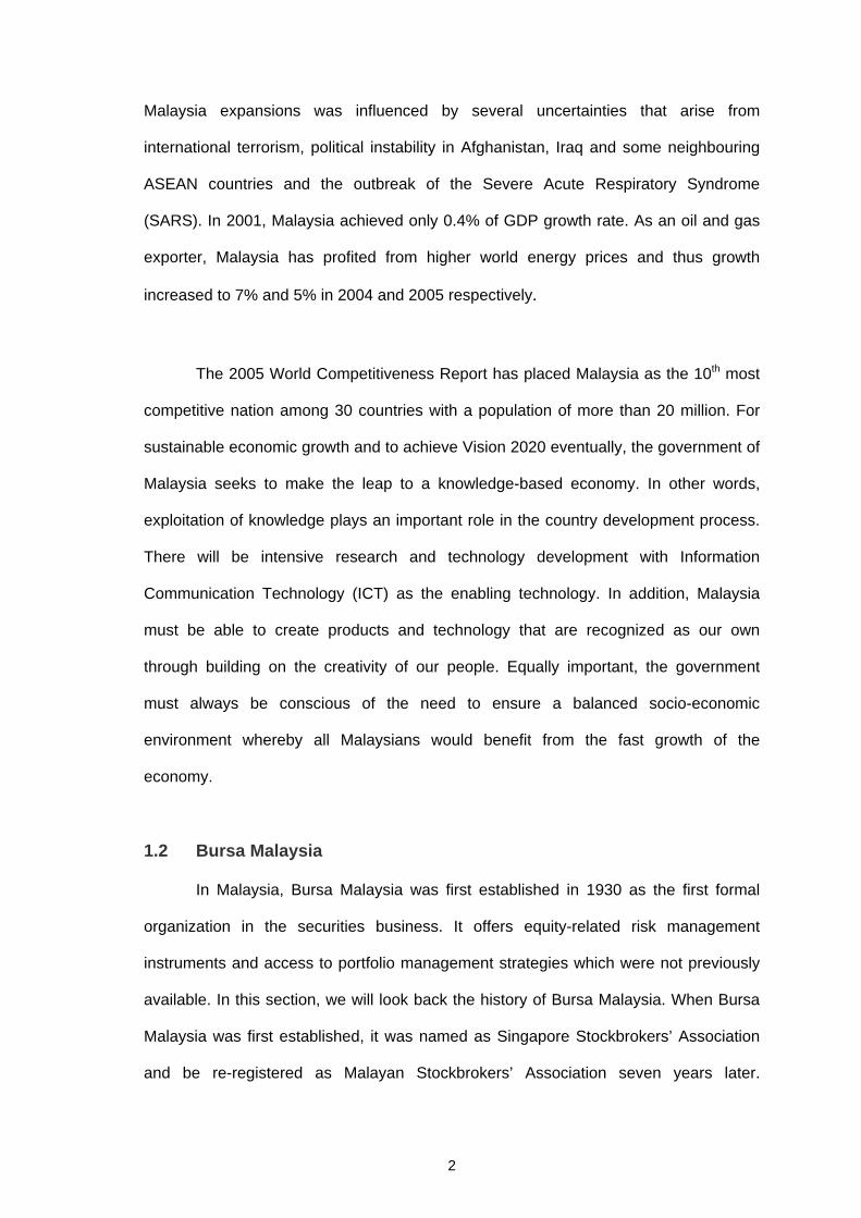
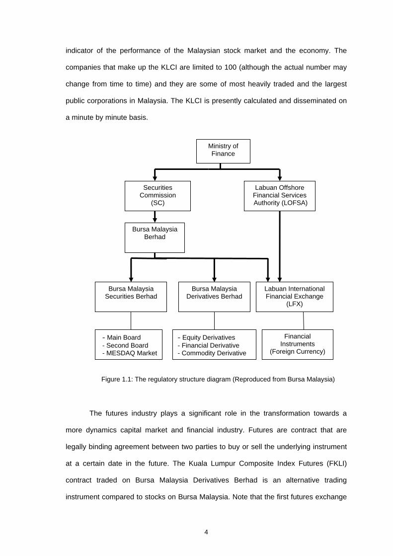
Figure 1.1 shows regulatory structure of Bursa Malaysia. Bursa Malaysia
operates under the supervision of the Securities Commission which falls under the
authority of the Ministry of Finance of Malaysia. This offers investors the security of
trading on a regulated exchange with similar rules and regulations like other stock
exchanges. Bursa Malaysia plays an important role as a central market place to
manage people risk exposure and to offer a competitive market place for fund raising
and investment. In addition, it is also a central market place for various types for
securities transactions between buyers and sellers. Bursa Malaysia was fully
computerized in 1992 with the introduction of System on Computerized Order Routing
and Execution (SCORE) automated trading system.
Bursa Malaysia computes an index for each of the main sectors traded on the
bourse but the most widely used performance index is by far the Kuala Lumpur
Composite Index (KLCI). It was introduced in 1986 since then it serves as an accurate
3
indicator of the performance of the Malaysian stock market and the economy. The
companies that make up the KLCI are limited to 100 (although the actual number may
change from time to time) and they are some of most heavily traded and the largest
public corporations in Malaysia. The KLCI is presently calculated and disseminated on
a minute by minute basis.
Securities Commission
(SC)
Labuan Offshore Financial Services Authority (LOFSA)
Bursa MalaysiaBerhad
Labuan International Financial Exchange
(LFX)
Bursa Malaysia Derivatives Berhad
Bursa Malaysia Securities Berhad
Financial Instruments
(Foreign Currency)
- Equity Derivatives - Financial Derivative - Commodity Derivative
- Main Board - Second Board - MESDAQ Market
Ministry of Finance
Figure 1.1: The regulatory structure diagram (Reproduced from Bursa Malaysia)
The futures industry plays a significant role in the transformation towards a
more dynamics capital market and financial industry. Futures are contract that are
legally binding agreement between two parties to buy or sell the underlying instrument
at a certain date in the future. The Kuala Lumpur Composite Index Futures (FKLI)
contract traded on Bursa Malaysia Derivatives Berhad is an alternative trading
instrument compared to stocks on Bursa Malaysia. Note that the first futures exchange
4
in Southeast Asia, Kuala Lumpur Commodity Exchange (KLCE) was establishment in
July 1980. This is then followed by the establishment of Kuala Lumpur Options and
Financial Futures Exchange (KLOFFE) which introduces the Kuala Lumpur Composite
Index Futures (FKLI) in 1995. With the introduction of FKLI, Malaysia became the third
Asian economy after Hong Kong and Japan to offer domestic equity derivatives
products. In June 2001, KLOFFE merged with the Commodity and Monetary Exchange
of Malaysia (COMMEX) and become Malaysian Derivative Exchange Berhad (MDEX).
MDEX
Trading Members
Local Members
Trading Permit Holders
Market Makers
Futures Brokers Representatives
Clients
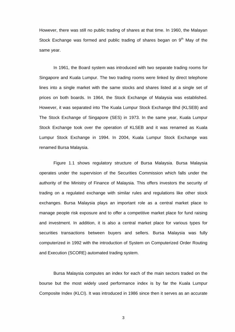
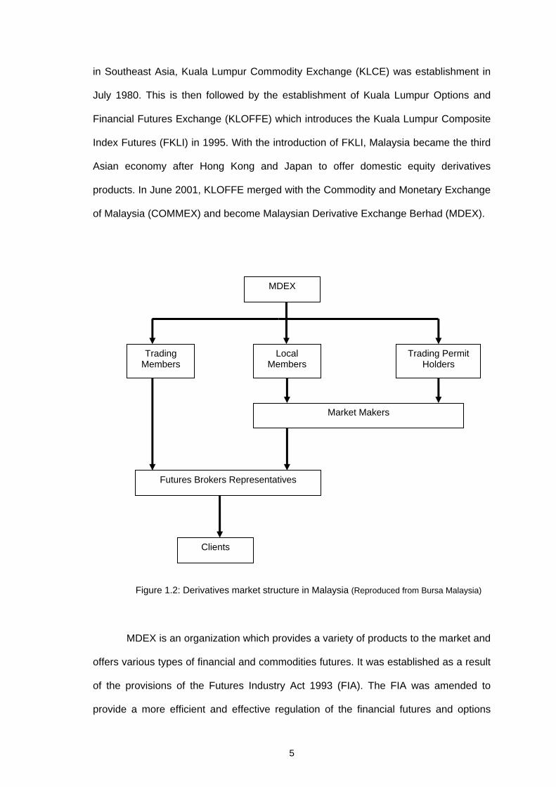
Figure 1.2: Derivatives market structure in Malaysia (Reproduced from Bursa Malaysia)
MDEX is an organization which provides a variety of products to the market and
offers various types of financial and commodities futures. It was established as a result
of the provisions of the Futures Industry Act 1993 (FIA). The FIA was amended to
provide a more efficient and effective regulation of the financial futures and options
5
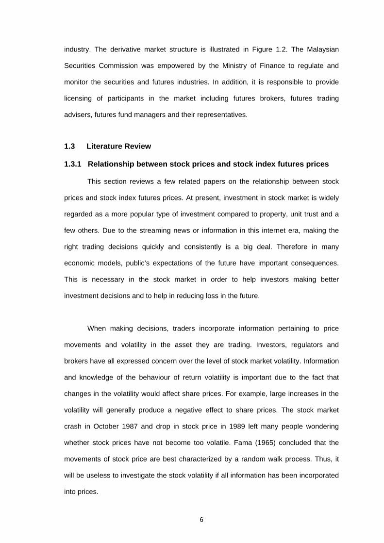
industry. The derivative market structure is illustrated in Figure 1.2. The Malaysian
Securities Commission was empowered by the Ministry of Finance to regulate and
monitor the securities and futures industries. In addition, it is responsible to provide
licensing of participants in the market including futures brokers, futures trading
advisers, futures fund managers and their representatives.
1.3 Literature Review
1.3.1 Relationship between stock prices and stock index futures prices This section reviews a few related papers on the relationship between stock
prices and stock index futures prices. At present, investment in stock market is widely
regarded as a more popular type of investment compared to property, unit trust and a
few others. Due to the streaming news or information in this internet era, making the
right trading decisions quickly and consistently is a big deal. Therefore in many
economic models, public’s expectations of the future have important consequences.
This is necessary in the stock market in order to help investors making better
investment decisions and to help in reducing loss in the future.
When making decisions, traders incorporate information pertaining to price
movements and volatility in the asset they are trading. Investors, regulators and
brokers have all expressed concern over the level of stock market volatility. Information
and knowledge of the behaviour of return volatility is important due to the fact that
changes in the volatility would affect share prices. For example, large increases in the
volatility will generally produce a negative effect to share prices. The stock market
crash in October 1987 and drop in stock price in 1989 left many people wondering
whether stock prices have not become too volatile. Fama (1965) concluded that the
movements of stock price are best characterized by a random walk process. Thus, it
will be useless to investigate the stock volatility if all information has been incorporated
into prices.
6
Although stock and futures prices may wander widely, the two series may share
the same stochastic trend since stock is the underlying asset for the futures. If so, the
series are cointegrated and are not expected to drift too far apart. The relationship
between stock index and stock index futures prices is critical because it has
implications regarding predominant financial theory, including market efficiency. Many
studies have examined how price movements are correlated across asset and
derivative security markets. In the last couple of decades, the relationship between
stock index and stock index futures markets has been the interest to academicians,
regulators and practitioners. Therefore, a number of studies have been conducted
ranging from developed markets to less developed markets. Nonetheless, the
sensitiveness of the relationship varies depending on the period of studies and the
occurrence of economic crisis or structural change in the data period.
Brooks et. al. (2001) showed that the return on a spot market index and
associated futures contract should be perfectly and contemporaneously correlated if
the respective markets are perfectly efficient. According to the efficient market
hypothesis, any mispricing in the market would be adjusted to eliminate any arbitrage
opportunities. Hence, the stock prices and futures will simultaneously reflect new
information in the market and no arbitrage profit can be made from the markets.
The theoretical relationship between a stock index and futures prices and its
underlying asset is presented by:
( )( )−( )( ) −⎡ ⎤= − − =⎣ ⎦exp r d MD tt t tF S r d MD t S e
tF
t
where:
= stock index futures prices quoted at time t
S = value of the underlying stock index at time t
7
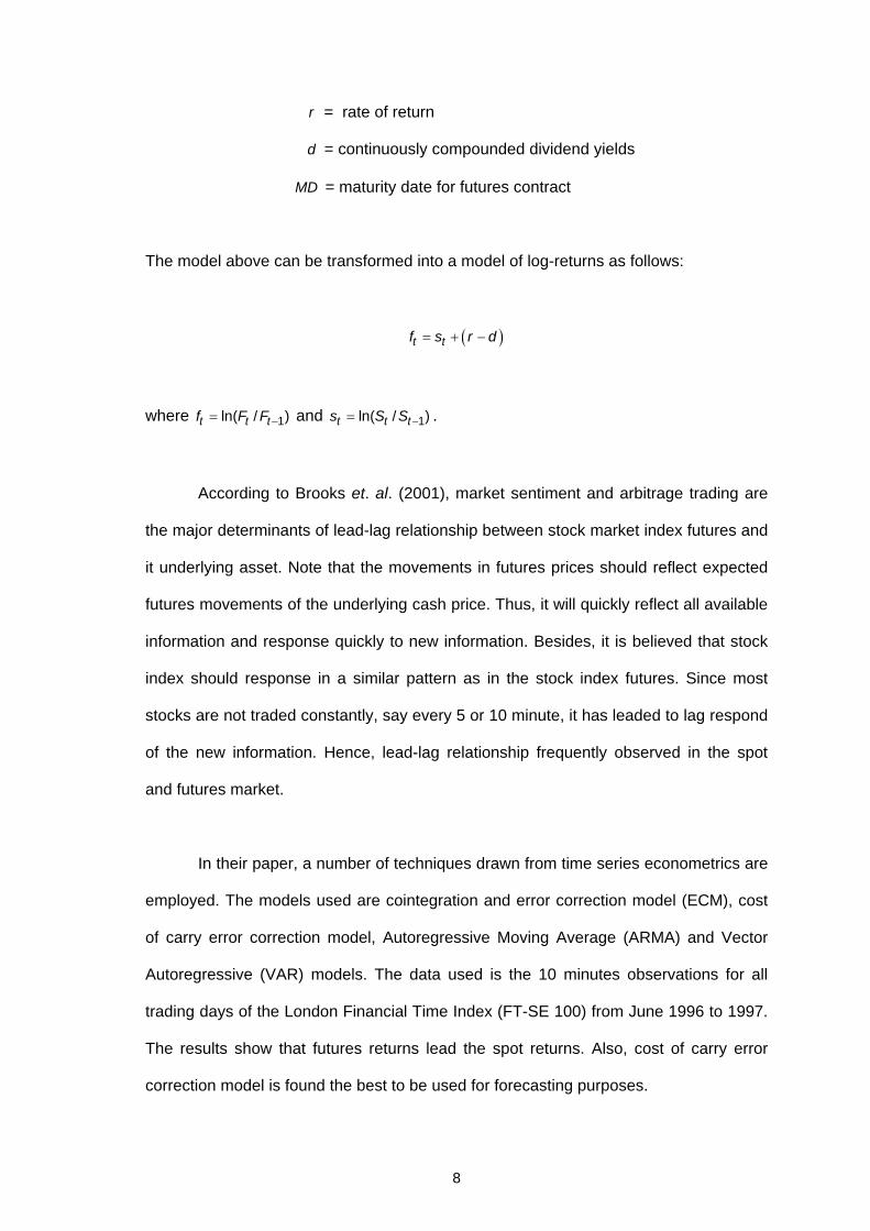
= rate of return r
= continuously compounded dividend yields d
MD = maturity date for futures contract
The model above can be transformed into a model of log-returns as follows:
( )t tf s r d = + −
1ln( / )t t tF −= 1ln( / )t t ts S S
where f F and −= .
According to Brooks et. al. (2001), market sentiment and arbitrage trading are
the major determinants of lead-lag relationship between stock market index futures and
it underlying asset. Note that the movements in futures prices should reflect expected
futures movements of the underlying cash price. Thus, it will quickly reflect all available
information and response quickly to new information. Besides, it is believed that stock
index should response in a similar pattern as in the stock index futures. Since most
stocks are not traded constantly, say every 5 or 10 minute, it has leaded to lag respond
of the new information. Hence, lead-lag relationship frequently observed in the spot
and futures market.
In their paper, a number of techniques drawn from time series econometrics are
employed. The models used are cointegration and error correction model (ECM), cost
of carry error correction model, Autoregressive Moving Average (ARMA) and Vector
Autoregressive (VAR) models. The data used is the 10 minutes observations for all
trading days of the London Financial Time Index (FT-SE 100) from June 1996 to 1997.
The results show that futures returns lead the spot returns. Also, cost of carry error
correction model is found the best to be used for forecasting purposes.
8
Wahab and Lashgari (1993) investigated the daily price-change in stock index
and stock index futures markets using cointegration and causality analysis. The data
employed in the study are daily closing spot and futures price for both the New York
Standard and Poor 500 index (S&P) and London FT-SE 100 index started from 4th
January 1988 to 30th May 992. The results show that cash and futures are
cointegrated. Morever, spot and futures price appear to be mostly simultaneously
related on a daily basis and this is generally consistent with the notion of market
efficiency. They also found that significant feedback exists between the cash and
futures for both the S&P 500 and London FT-SE 100 indexes. However, the spot-to-
futures lead appears to be more pronounced across days relative to the futures-to-spot
lead. In addition, it is known that futures prices exhibit stronger subsequent response to
disequilibrium in the spot prices and conversely, this does not apply to the spot prices
towards last period’s futures equilibrium error.
Ghosh (1993) investigated the relationship between spot and futures price using
Dickey-Fuller cointegration test and error correction model. There are two data set
used in the study: Standard and Poor’s (S&P) 500 spot index and intra-day futures
price as well as daily closing prices of Commodity Research Bureau (CRB) spot index
and near term delivery of futures covering the time period from January 1988 to
December 1988 and 12th June 1986 to 31st December 1989 respectively. The results
show that both systems are cointegrated and therefore exhibit stable long-run
equilibrium relationship. The error correction models are shown to be statistically
significant in most cases. It is found that the disequilibrium in one period is corrected in
the next period. For the S&P index, log of current spot price depends to a great extent
on futures prices. However, the opposite occurrence is seen for the CRB index. The
forecasting performance from error correction model outperforms the naïve model
using the Ordinary Least Squared (OLS) regression. The result suggests that this
modeling strategy offers potential for forecasting prices changes.
9

Iihara et. al. (1996) examined time series properties of intraday returns for stock
index and stock index futures in Japan. The data set contains the time of transaction
and the price for every futures transaction as well as the Tokyo Nikkei Stock Average
(NSA) index from March 1989 to February 1991. There are three distinct time periods
in the sample. The first period includes the year 1989 (bull market), the second year
includes the year 1990 until the introduction of the stricter measures (bear market)
while the third year begins after the introduction of the stricter measures and continues
to March 1991 (bear market). The reason for this partition is due to the change in stock
market condition. During the first period of bull market, the stock prices generally
increase and achieve its highest value while during the second period of bear market,
the stock prices generally decrease.
Lead-lag relationship between the intraday returns is investigated using
regression technique. The results show that the introduction of stricter measures
increase the volatility of both index and futures prices. At the same time, the speed of
information dissemination in the futures markets is reduced. This suggests that futures
returns strongly leads cash returns for all three periods. In term of volatility, there is no
bi-directional information flows between the cash and futures markets. However, it is
found that the futures market shocks significantly affect the conditional volatility of the
cash market before the stricter measures are introduced. In other words, the stricter
measures appear to reduce the information flow from the futures to the cash market. In
addition, results show that the inter-market dependence of conditional volatilities is
insignificant. Past conditional volatility affects only the current conditional volatility of its
own market.
Marie and Lucy (1998) adopted the multivariate Generalized Autoregressive
Heteroscedasticity (GARCH-M) model to examine relationship between stock indices
and the associated futures prices. The study also provides evidence concerning day-of-
10
week and holiday effects on price movement and volatility. There are three series used
in the paper including the New York Stock Exchange Composite, S&P 500 and Toronto
35. The data consists of daily observations for the three indices and their futures prices
from January 1998 to March 1993.
The paper suggested that the GARCH-M model provides useful information
concerning the movement of asset prices over time. The paper jointly models first and
second moments of the price processes across markets. At the same time, seasonal
effects are allowed in the model. The results show that seasonal effects are not
consistently reflected in price movement and volatility. In general, the results provide
significant evidence of time variation in price volatility and correlation in volatility across
stock and futures markets. It is shown that the time-varying volatilities are significantly
and positively correlated for the North American markets. This is mostly due to the fact
that Canada and United States share similar market structures and regulatory
environment. As expected, the volatility correlations decrease over time.
Wong and Meera (2001) studied the market efficiency in Malaysia stock index,
KLCI and futures market, FKLI. Methodologies employed in the paper are Granger
causality and error correction approach. The data are divided into two sub-samples:
before financial crisis, from January 1996 to March 1997 and during the financial crisis,
from April 1997 to September 1998. The results show that KLCI price lead FKLI before
the economic crisis but not vice versa. In addition, there is no long run equilibrium
relationship between both markets.
Chan and Karim (2004) analyse the lead lag relationship between spot and
futures market of the KLCI. They used cointegration and error-correction model in their
analysis. Daily closing price from January 1996 to December 2002 is used. It is
suggested that KLCI prices and the corresponding futures markets are cointegrated.
11
Also, it is proven that futures prices can be a good indicator on predicting spot prices
due to the stronger impacts of futures prices on cash markets compared to that from
cash market to futures market. There are many other studies that have investigated the
lead-lag relationship between futures market and cash market. These includes Lim
(1992) who found that there is no lead-lag relationship between the Tokyo Nikkei Stock
Average (NSA) stock and futures markets. Tang et. al. (1992) suggested that Hang
Seng Index Futures cause the spot index prices to change during the pre-crash period
but not vice-versa. However, there is a bi-directional relationship between the two
variables during the post-cash period.
1.3.2 Relationship between stock prices and foreign exchange rates
Since stock market provides an ideal investment opportunity for local company
as well as for foreign company, there is a strong correlation between a country’s stock
market and its currency. A currency is a unit of exchange, facilitating the transfer of
goods and services. A currency zone is a country or region in which a specific currency
is the dominant medium of exchange. To facilitate trade between currency zones, there
are exchange rates i.e. prices at which currencies (and the goods and services of
individual currency zones) can be exchanged against each other. Modern currencies
can be classified as either floating currencies or fixed currencies based on their
exchange rate regime.
Changes in the international and regional financial as well as the economic
environment have made it important for Malaysia to have a stable exchange rate. To
achieve stability of exchange rate, our government has to maintain the value of Ringgit
against the currencies of its major trading partners. The United Kingdom has the fifth
largest economy in the world in terms of market exchange rates. Its currency, Pound
Sterling is one of the highest valued currencies among the major currency units in the
world. Therefore it is believed that the UK’s economy is associated with many other
12
capitalist economies in the world and thus Pound Sterling has a close relationship with
most of the world stock markets including Malaysia. When the currency is bought, its
value will rise. On the other hand, the currency will fall when it is sold.
Fluctuations in the currency can affect the values of firms and the structure of
financial markets. Besides, it also affects people’s investment and financial decisions.
Consequently, it brings a huge impact to a country’s stock market and thus the
economy development. Studies show that, in the long run, exchange rates are
determined by current and future economic fundamentals. These fundamentals include
interest rates, inflation and money supplies. However, in the short run, exchange rates
are also affected by other factors such as political stability and changes of policy.
Exchange rates play the role of balancing the demand for and supply of assets.
An increase in domestic stock prices lead individuals to demand more domestic assets.
To buy more domestic assets local investors would sell foreign assets (they are
relatively less attractive now), causing local currency appreciation. In addition, a
blooming stock market would attract capital flows in from foreign investors, which may
cause an increase in the demand for a country’s currency. As a result, rising (declining)
stock prices would lead to an appreciation (depreciation) in exchange rates.
The issue regarding relationship between stock price and exchange rates has
received considerable attention especially after the East Asian crisis. If these two
macroeconomic variables are related then investors can predict the behaviour of one
variable based on the information of another variable. If the causation runs from
exchange rates to stock prices then crises in the stock markets can be prevented by
controlling the exchange rates. Similarly, if the causation runs from stock prices to
exchange rates then authorities can focus on domestic economic policies to stabilize
the stock market.
13
For the past few decades, many works have been carried out to examine the
relationship between stock prices and exchange rate. However, most of the attention
has been focused on developed countries. The results of these studies are
inconclusive as some studies have found a significant positive relationship between
stock prices and exchange rates while others have reported a significant negative
relationship between the two variables. On the other hand, there are some studies that
have found very weak or no association between stock prices and exchange rates. In
general, there is clearly neither a theoretical nor empirical consensus on the
relationship between exchange rates and stock prices.
Baharumshah et. al. (2002) presented and tested an augmented monetary
model that includes the effect of stock prices on the bilateral exchange rates. The
model is given as follows:
* * * *
0 1 2 3 4( ) ( ) ( ) ( )t t t t t t t t t te β β m m β y y β i i β s s u= + − + − + − + − +
1 0β > 2 0β < 3 0β > t
m
where , and . Note that e is the log of the exchange rate (defined
as the domestic price of foreign currency), is the nominal demand for money, y is
the real income level, is the nominal rate of interest, is the real level of the stock
market and u is a random error term. The asterisk (*) denotes the corresponding
foreign variables.
i s
t
In Baharumshah et. al. (2002), the exchange rates and the macroeconomic
variables from the first quarter in 1976 to the forth quarter in 1996 are used. By defining
Malaysia (RM) as the home country whereas US (US) and Japan (JY) as the foreign
countries, the RM/US and the RM/JY exchange rates are used. The income variable is
measured by real gross domestic product, money supply is represented by M1 (a
measure of money supply including all coins, notes and personal money in current
14
accounts) and the stock market is represented by the main stock index. Besides, short-
run interest rate of 3-month Treasury bill is also used in the analysis.
The analysis is carried out by using Johansen method of cointegration and a
restricted VAR model by Sims (1990). The initial results show that the monetary
variable is cointegrated but it is subjected to parameter instability. The time-varying
parameter is found affecting at least a particular subset of the variables in the system
including the stock prices. The analysis is then continued by using VAR model which
imposes exogeneity restrictions on the first order integrated, Ι variables. The result
shows existence of cointegration and parameter stability. It suggests that the equity
market significantly affect the exchange rate and hence models of equilibrium
exchange rate should be extended to include equity markets in addition to bond
markets. The study also indicates that factors affecting the equity price are likely to
influence the movement of exchange rates.
(1)
Granger et. al. (2000) applied unit root test and cointegration model to
investigate the relationship between stock prices and exchange rates. Since the
Augmented Dickey Fuller (ADF) test is suspected when sample period includes
structural breaks or major events such as great depression and stock market crash, the
authors introduced a dummy variable into the original ADF formula as suggested by
Perron and Vogelsang (1992):
1
11
∆ ( 1) ( ) ∆k
t t t i t i ti
y α βt ρ y γDU λ θ y a−
− −=
= + + − + + +∑
1 L= − t, where ∆ y is a macroeconomic variable, t is a trend variable and is a white
noise term. For
ta
t Nλ> ( ) 1t λ, DU = , otherwise ( ) 0tDU λ = , /λ BT N= is the location where
the structural break lies, N is sample size and T is the date when structural break
occurred.
B
15
Data used in the study are exchange rates and stock prices from some Asian
countries, namely Hong Kong, Indonesia, Japan, South Korea, Malaysia, the
Philippines, Singapore, Thailand and Taiwan. Daily data from 3rd January 1996 to 16th
June 1998 are taken and are divided into three sub-samples i.e. crash, after crash and
the Asian flu period.
Before the crash period (1986-1987), there is little interaction between currency
and stock markets except for Singapore where changes in the exchange rates lead the
stock price. In the period after crash, there is no definite pattern of interaction between
the two markets. However, seven of the nine nations including Malaysia suggest
significant relations between the two markets during the Asian flu period. The impulse
response analysis lends further support to the importance of stock market as the leader
or the existence of feedback interaction during the Asian flu period.
Nieh and Lee (2001) investigated the dynamic relationship between stock prices
and exchange rates for G-7 countries. Data consists of daily closing stock market
indices and foreign exchange rate from 1st October 1993 to 15th February 1996. The
analysis is carried out using Engle-Granger (1987) two steps method and the Johansen
maximum likelihood cointegration test. The appropriate framework of Vector Error
Correction model (VECM) is further applied to assess both the short-run inter-temporal
co-movement between the two variables and their long-run equilibrium relationship.
The paper also incorporates Johansen’s (1988, 1990 and 1994) five VECM models to
consider the determinant of cointegrating ranks in the presence of a linear trend and a
quadratic trend.
The results reject most of the previous studies that suggest a significant
relationship between stock prices and exchange rates. Their result is similar to that
suggested by Bahmani-Oskooee and Sohrabian (1992) finding where there is no long-
16
run significant relationship between stock prices and exchange rates for each G-7
countries. Additionally, result from the VECM estimation suggests that the two lead-
lagged length of one financial variable has little power in predicting the other. The result
shows that these two financial variables do not show predictive capabilities for more
than two consecutive trading days. In other words, only one day’s short run significant
relationship has been found in certain G-7 countries. Another finding from the study is
that the US fails to show any significant correlation and thus the value of dollar cannot
be used to predict the future in the US.
Phylaktis and Ravazzolo (2005) examined both the long-run and short-run link
between stock prices and exchange rates in a group of Pacific Basin countries
including Hong Kong, Malaysia, Singapore, Thailand and the Philippines. The main
concern of the study is to investigate whether any relationship is affected by the
existence of foreign exchange controls and by the Asian financial crisis in the middle of
1997. The sample period covered from 1980 to 1998 and it varies for each country
depending on the availability of data. By using cointegration and multivariate Granger
causality tests, the study suggests that stock and foreign exchange markets are
positively related and that the US stock market acts as a medium for these links.
Furthermore, the relationship between stock and foreign exchange markets are found
not to be affected by foreign exchange restrictions. Besides, it is shown that the
financial crisis had a temporary effect on the long-run co-movement of these markets.
Wu (2001) analyses the symmetric asset-price movements in Singapore by
using a monetary approach. The relative magnitudes of the exchange rate elasticity of
real money demand and that of real money supply determine the relations between
stock prices and exchange rates. The results show that if the demand for real money
balances is relatively exchange-rate elastic, exchange rate and stock prices are
negatively related, and if the overall price level and thus real money supply is relatively
17
exchange-rate elastic, the opposite holds. The results also reveal that the interest rate
is positively related to stock prices when the demand for real money balances is more
exchange-rate elastic than the real money supply, and vice versa.
In addition, the distributed lag model and the VAR model are used to analyse
the Straits Times Industrial Index’s macroeconomic exposure (STII) both before and
during the 1997 Asian financial crisis periods. It is suggested that fiscal revenues and
fiscal expenditures exert positive influences on stock prices for both the investigated
periods. Morever, a positive interest rate shock tends to boost the stock prices during
the crisis period. It is also found that the Singapore dollar has bi-directional relationship
with currencies of developed countries, except Singapore dollar-Malaysian Ringgit are
negatively related with the STII both before and during the 1997 Asian financial crisis.
Finally, the results imply that the real money demand is relatively exchange-rate elastic
with respect to the rich country’s currencies but relatively inelastic with respect to the
Malaysian Ringgit when compared to the real money supply.
Ibrahim (2003a) applied cointegration and VAR modeling to evaluate the long-
run relationship and dynamic interactions between the Malaysian equity market,
various economic variables and major equity markets of the US and Japan. The stock
indices used are KLCI, S&P 500 and Nikkei 225 Index from January 1977 to August
1998. The variance decompositions and impulse-response functions generated from
the VAR suggest dominant influence of nominal variables on Malaysian equity prices. It
is noted that KLCI positively related to money supply, consumer price index and
industrial production index but it is negatively linked to the exchange rate. At the same
time, variations in equity prices do contain some information on such nominal variable,
implying bi-directional causality between them. Besides, it is found that the nature of
long-run relationships in the Malaysian and Japan equity market are similar but they
are different from that of the US market. The possible explanation is that Malaysia and
18

Japan are considered as one East Asian market whereas the US market is an
alternative market.
1.3.3 Application of Kalman filter technique (KF) and Generalized Autoregressive Conditional Heteroskedaticity (GARCH)
Ever since its development by Kalman and Bucy in early 1960s, the Kalman
filter technique has played an important role in the space programme and has become
an important tool for many analyses in control engineering. This may be due to difficulty
in understanding different terminology in control engineering, statistics and economy.
However, its applications in statistics and economics have been very few and far in
between. The Kalman filter is useful for parameter estimation and inference about
unobserved variables in linear dynamic systems. It is a basic technique relates to the
state-space model. The following section discusses the applications of the Kalman filter
technique in econometrics and time series analysis.
Arsad (2002) makes use of Kalman filtering technique to analyse state-space
model extensions of the Wilkie stochastic asset model. A model for the United Kingdom
Retail Price Index (RPI) is proposed and investigated. The rate of inflation and its mean
reversion level are allowed to be modeled stochastically. The proposed model is
compared to the simpler Wilkie Autoregressive, AR(1).
In addition, the Kalman filter technique is applied to a combined series of price
inflation, equity dividend yields and dividend growth rates. The dynamics between
equity dividend yields and dividend growth rates with the future rate of inflation are
investigated respectively. Through the state-space form of the Kalman filter, an
unobserved series is introduced into the structure of the model.
19
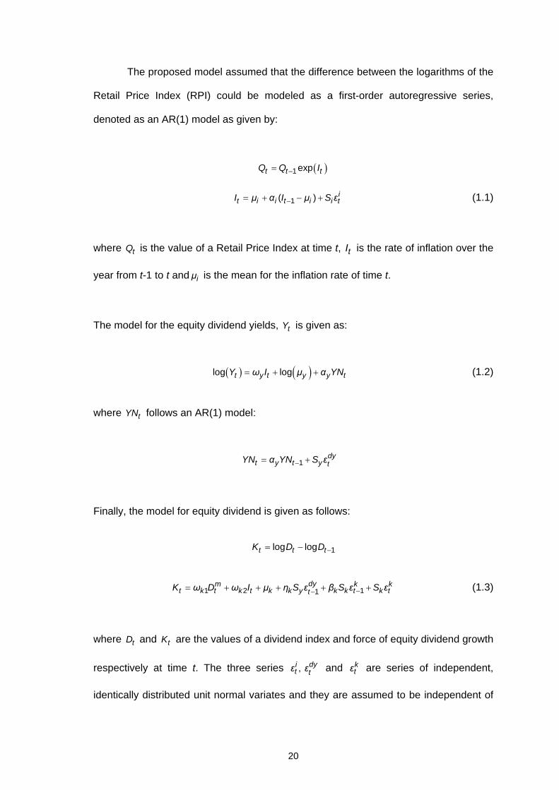
The proposed model assumed that the difference between the logarithms of the
Retail Price Index (RPI) could be modeled as a first-order autoregressive series,
denoted as an AR(1) model as given by:
( )1 expt t tQ Q I−=
1( ) it i i t i i tI μ α I μ S ε−= + − +
t tI
iμ
t
( )
(1.1)
where Q is the value of a Retail Price Index at time t, is the rate of inflation over the
year from t-1 to t and is the mean for the inflation rate of time t.
The model for the equity dividend yields, Y is given as:
( )log logt y t y y tY ω I μ α YN= + +
t
1 dyt y t y tYN α YN S ε−= +
1log logt t tK D D
(1.2)
where YN follows an AR(1) model:
Finally, the model for equity dividend is given as follows:
−= −
k kK ω
it
1 2 11dym
t k t k t k k y k k t k ttD ω I μ η S ε β S ε S ε−−= + + + + + (1.3)
where and are the values of a dividend index and force of equity dividend growth
respectively at time t. The three series and are series of independent,
identically distributed unit normal variates and they are assumed to be independent of
tD Kt
, dytε ε k
tε
20
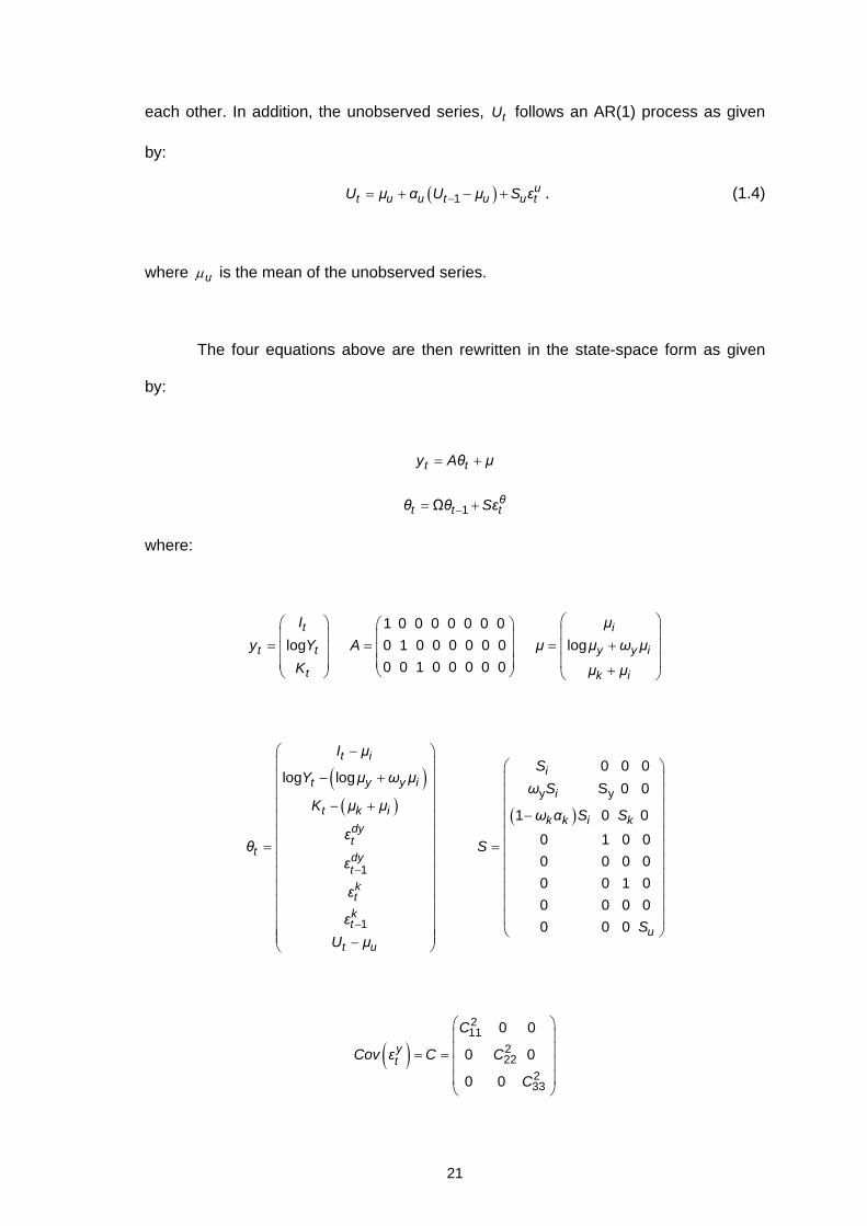
each other. In addition, the unobserved series, follows an AR(1) process as given
by:
tU
( )u1u
t u u t u tU μ α U μ S ε−= + − + . (1.4)
where uμ is the mean of the unobserved series.
The four equations above are then rewritten in the state-space form as given
by:
t ty Aθ μ= +
1Ωt t tθ θ −= +
1 0 0 0 0 0 0 0log 0 1 0 0 0 0 0 0 log
0 0 1 0 0 0
t i
t t y y i
t k i
I μy Y A μ μ ω μ
K μ μ
⎛ ⎞⎛ ⎞⎜ ⎟⎜ ⎟
= = = +⎜ ⎟⎜ ⎟⎜ ⎟⎜ ⎟ +⎝ ⎠ ⎝ ⎠
( )( ) ( )
y y
1
1
0 0 0log log
S 0 0
1 0 0 0 1 0 0
t ii
t y y ii
t k ik k i k
dyt
t dytktkt
t u
I μS
Y μ ω μω S
K μ μω α S S
εθ S
ε
ε
εU μ
−
−
−⎛ ⎞⎜ ⎟
− +⎜ ⎟⎜ ⎟
− +⎜ ⎟−⎜ ⎟
⎜ ⎟⎜ ⎟⎜ ⎟⎜ ⎟⎜ ⎟⎜ ⎟⎜ ⎟⎜ ⎟⎜ ⎟−⎝ ⎠
0 0 0 0 0 0 1 0 0 0 0 0
0 0 0 uS
⎛ ⎞⎜ ⎟⎜ ⎟⎜ ⎟⎜ ⎟⎜ ⎟⎜ ⎟⎜ ⎟⎜ ⎟⎜ ⎟⎜ ⎟⎜ ⎟⎝ ⎠
( )211
22233
0 0
0 0
yt
C
Cov ε C C
C
⎛ ⎞⎜ ⎟⎜ ⎟= =⎜ ⎟⎜ ⎟⎝ ⎠
θSε
0 0
⎛ ⎞⎜ ⎟⎜ ⎟⎜ ⎟⎝ ⎠
= =
2
0 0
where:
21
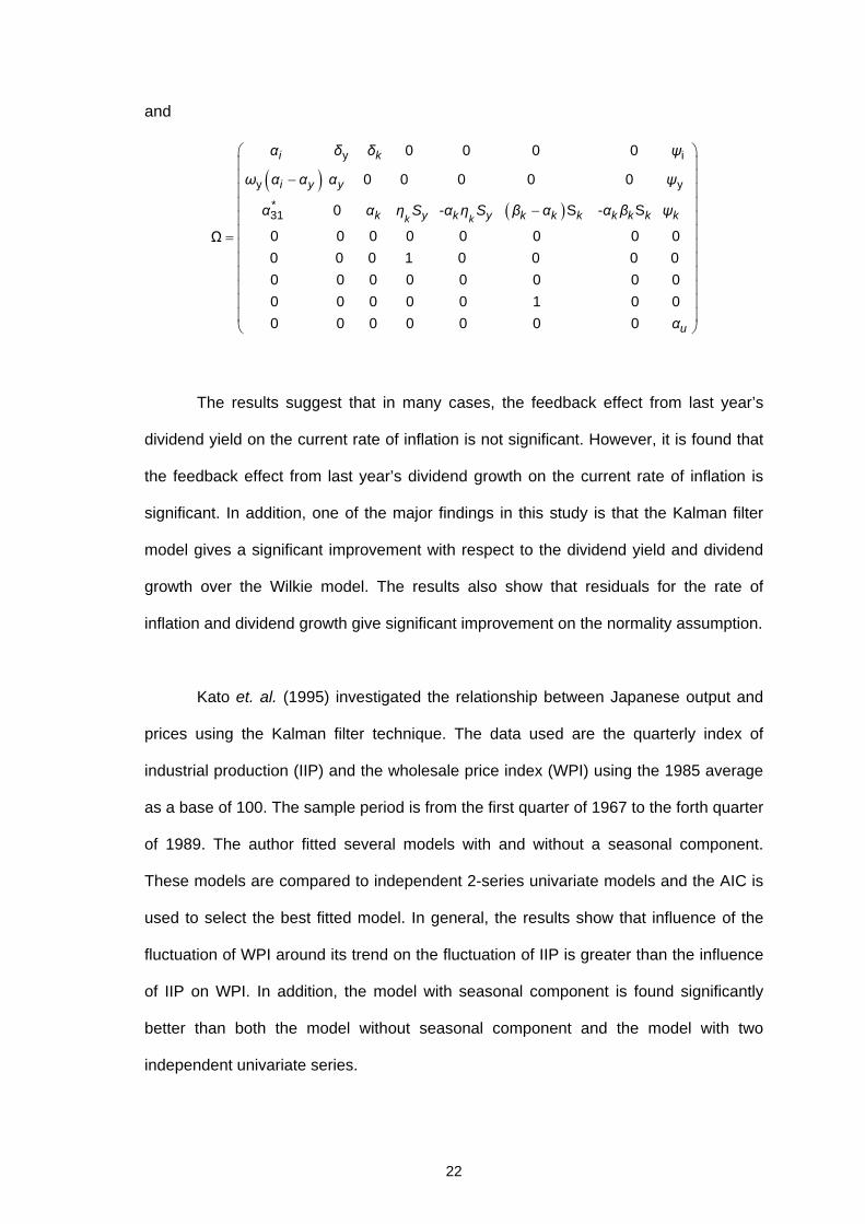
and
( )y i
y y
*31
0 0 0 0
0 0 0 0 0
Ω
i k
i y y
α δ δ ψ
ω α α α ψ
α
−
=
( ) 0 - S - S
0 0 0 0 0 0 0 0 0 0 0 1 0
k kk y k y k k k k k k kα η S α η S β α α β ψ−
0 0 0 0 0 0 0 0 0 0 0 0 0 0 0 0 1 0 0 0 0 0 0 0 0 0 uα
⎛ ⎞⎜ ⎟⎜ ⎟⎜ ⎟⎜ ⎟⎜ ⎟⎜ ⎟⎜ ⎟⎜ ⎟⎜ ⎟⎜ ⎟⎜ ⎟⎜ ⎟⎝ ⎠
The results suggest that in many cases, the feedback effect from last year’s
dividend yield on the current rate of inflation is not significant. However, it is found that
the feedback effect from last year’s dividend growth on the current rate of inflation is
significant. In addition, one of the major findings in this study is that the Kalman filter
model gives a significant improvement with respect to the dividend yield and dividend
growth over the Wilkie model. The results also show that residuals for the rate of
inflation and dividend growth give significant improvement on the normality assumption.
Kato et. al. (1995) investigated the relationship between Japanese output and
prices using the Kalman filter technique. The data used are the quarterly index of
industrial production (IIP) and the wholesale price index (WPI) using the 1985 average
as a base of 100. The sample period is from the first quarter of 1967 to the forth quarter
of 1989. The author fitted several models with and without a seasonal component.
These models are compared to independent 2-series univariate models and the AIC is
used to select the best fitted model. In general, the results show that influence of the
fluctuation of WPI around its trend on the fluctuation of IIP is greater than the influence
of IIP on WPI. In addition, the model with seasonal component is found significantly
better than both the model without seasonal component and the model with two
independent univariate series.
22
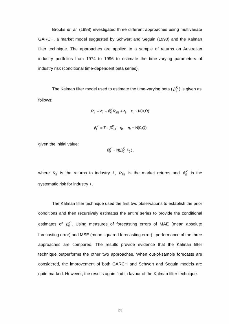
Brooks et. al. (1998) investigated three different approaches using multivariate
GARCH, a market model suggested by Schwert and Seguin (1990) and the Kalman
filter technique. The approaches are applied to a sample of returns on Australian
industry portfolios from 1974 to 1996 to estimate the time-varying parameters of
industry risk (conditional time-dependent beta series).
The Kalman filter model used to estimate the time-varying beta ( ) is given as
follows:
Kitβ
t, ~ N(0,Ω)Kit t it Mt tR α β R ε ε= + +
1 t, ~ N(0, )K Kt t tβ T β η η Q−= × +
0 0 0~ N( , )K Kβ β P
itR i MtR Kitβ
i
Kitβ
given the initial value: .
where is the returns to industry , is the market returns and is the
systematic risk for industry .
The Kalman filter technique used the first two observations to establish the prior
conditions and then recursively estimates the entire series to provide the conditional
estimates of . Using measures of forecasting errors of MAE (mean absolute
forecasting error) and MSE (mean squared forecasting error) , performance of the three
approaches are compared. The results provide evidence that the Kalman filter
technique outperforms the other two approaches. When out-of-sample forecasts are
considered, the improvement of both GARCH and Schwert and Seguin models are
quite marked. However, the results again find in favour of the Kalman filter technique.
23
Morris and Pfeffermann (1984) applied the Kalman filter technique to monthly
time series which are affected by moving festivals. The model used to forecast festivals
which do not fall on the same date in the Gregorian calendar from year to year.
Examples of these festivals are the Passover in Israel, Easter weekend and the
Chinese New Year.
The model is applied to three different series including Taiwan traffic volume
(1963-1976), Israel work seekers (1962-1981) and Israel tourist arrivals (1960-1982).
Below is the proposed model:
( )t
t t t ty
t tt t
y A θ ε
μ ρ F φ ε
= +
+ + +l
-1Ω θt t tθ θ ε
=
= +
where
( )(12) (11) (1)t t ... T
t t t t tθ μ β p p p φ=
( )1 0 0 ... 0 0 1 t tA F=
~ N(0, ), ~ N(0, )yθt t ttε R ε C
tμ tβ tF
tφl( )
t
and are the levels and slope of the process at time month t respectively, is
the festival coefficient for month t, is the festival parameter for month t and ρ is
the seasonal effect associated with calendar month prior to the current month. ( +1)l
For the first series, it is assumed that the New Year affects a ten day period
starting three days before the festival and that the extra traffic is distributed evenly
throughout this period. The results show that there is a considerable increase in traffic
volume around the date of the Chinese New Year from 21st January to 17th February.
24

In addition, both Passover (26th March to 25th April) and the Jewish New Year (6th
September to 5th October) are believed to significantly affect the second and third
series respectively. It is also assumed that the Passover affects a twenty-three day
period starting seventeen days before the festival and that the New Year affects a thirty
day period starting five days before the festival.
Li (2000) investigated the efficiency of China’s stock markets by examining the
changing behavior over the entire history of the Shenzhen and Shanghai Stock
Exchanges. Daily data from January 1991 to January 2001 is used. The Kalman filter
technique is applied to a combination of time-varying AR (2) model and an asymmetric
ARCH equation as given by:
0 1 1 2 2t t t t t t t− −
2, ~ N(0, ), 0β β u u σ i= + =
, ~ N(0,t tR β β R β R e e h= + + + )
1t
(1.5)
1 , 1, 2it it it it i− (1.6)
where is the rate of daily stock returns at time t and is normally distributed with
zero mean and conditional variance . The autoregressive coefficients in Equation
(1.5) are assumed to follow a random walk processes. The time-varying values of
help to reflect the changing degree of predictability of stock market.
tR te
th
itβ
Three alternative ARCH models are used and the conditional variance, is
given below:
th
2 2
0 1 1 2 1 3t t th α α e D α e D α h− + − −= + + + − (1.7)
2 22 1te D0 1 1 3t th γ γ e γ γ h 1t− − − −= + + + (1.8)
1 1
0 1 2 3 11 1
ln lnt tt t
t t
e eh θ θ θ θ h
h h− − (1.9) −− −
= + + +
25