Dynamic Predictive Density Combinations

for Large Data Sets in Economics and Finance∗

Roberto Casarin† Stefano Grassi§

Francesco Ravazzolo‡ Herman K. van Dijk¶

†University Ca’ Foscari of Venice

‡Norges Bank and Centre for Applied Macro and Petroleum economics

at BI Norwegian Business School

§University of Kent

¶Econometric Institute Erasmus University Rotterdam, Econometrics Department

VU University Amsterdam and Tinbergen Institute

May 2015

Abstract

A Bayesian nonparametric predictive model is introduced to construct time-

varying weighted combinations of many predictive densities for large data sets. A

parallelized clustering mechanism allocates the predictive densities into a small

number of mutually exclusive subsets. A dynamic factor model is specified for

the weight transition density defined on a reduced dimension simplex using the

class-preserving property of the logistic-normal distribution. Density combination

weights are updated with parallel sequential Monte Carlo filters. The procedure

is applied to predict Standard & Poor’s 500 index using more than 7000

∗This working paper should not be reported as representing the views of Norges Bank. The viewsexpressed are those of the authors and do not necessarily reflect those of Norges Bank. We thankJohn Geweke, Jim Stock, Peter Schotman, Peter Hansen, Gael Martin, Michael Smith, AnastasiosPanagiotalis, Barbara Rossi and conference and seminar participants at Erasmus University RotterdamWorkshop on “The Econometric Analysis of Recurrent Events in Macroeconomics and Finance”, the34th International Symposium on Forecasting, the 8th International CFE meeting in Pisa, the 25thEC2 Conference on “Advances in Forecasting”, Institute for Advance Studies Vienna, MaastrichtUniversity, Monash University, Norges Bank, the Stevanovich Center at University of Chicago, UTSSydney, and UPF Barcelona, for very useful comments. Roberto Casarin’s research is supportedby funding from the European Union, Seventh Framework Programme FP7/2007-2013 under grantagreement SYRTO-SSH-2012-320270, by the Institut Europlace de Finance, Systemic Risk grant, andby the Italian Ministry of Education, University and Research (MIUR) PRIN 2010-11 grant MISURA.

1

predictive densities based on US individual stocks and finds substantial forecast

and economic gains. Similar forecast gains are obtained in point and density

forecasting of US real GDP, Inflation, Treasury Bill yield and employment using

a large data set. A Graphics Processing Unit type of algorithm reduces the

computing time considerably.

JEL codes: C11, C15, C53, E37.

Keywords: Density Forecast Combination, Large Set of Predictive Densities,

Compositional State Space, Bayesian Inference, GPU Computing.

1 Introduction

Forecasting with large sets of data is a topic of substantial interest to academic

researchers as well as to professional and applied forecasters. It has been studied in

several papers (e.g., see Stock and Watson, 1999, 2002, 2004, 2005, 2014, and Banbura

et al., 2010). The recent fast growth in (real-time) big data allows researchers to

predict variables of interest more accurately. Stock and Watson (2005, 2014), Banbura

et al. (2010) and Koop and Korobilis (2013) suggest, for instance, that there are

potential gains from forecasting using a large set of predictors instead of a single

predictor from a univariate time series. However, forecasting with many predictors

and high-dimensional models requires new modeling strategies (to keep the number

of parameters and latent variables relatively small), efficient inference methods and

extra computing power like parallel computing. We refer to Granger (1998) for an

early discussion of these issues.

In this paper we propose a Bayesian nonparametric predictive model that extends

substantially the general combination model given in Billio et al. (2013) and Casarin

et al. (2015) in order to deal with a high dimensional combination model that is

still relatively parsimonious in the number of parameters and latent variables. We

show that the proposed combination model has a natural representation in terms of

dependent sequence of random measures with common atoms and component-specific

weights. Our model extends the mixture of the experts and the smoothly mixing

regression models (Jacobs et al. (1991), Jordan and Jacobs (1994), Jordan and Xu

(1995), Peng et al. (1996), Wood et al. (2002), Geweke and Keane (2007), Villani

et al. (2009), Norets (2010)) by allowing for dependence between the random weights

of the mixture. In this sense, our combination model shares some similarities with the

dependent random measures used in Bayesian nonparametric models (see Muller and

Quintana (2010) and Muller and Mitra (2013)).

2

As regards the random weights, our model makes use of a clustering mechanism

where allocation variables map the original set of predictive densities into a relatively

small number of mutually exclusive subsets with combination weights driven by cluster

specific latent processes specified as a compositional factor model, see Pawlowsky-

Glahn and Buccianti (2011) for details on compositional data analysis. This structure

of the latent space allows for a probabilistic interpretation of the weights as model

probabilities in the combination scheme. There exists an issue of analytic tractability

of the probabilistic information in the information reduction step. Here the class-

preserving property of the logistic-normal distribution (see Aitchinson and Shen, 1980,

Aitchinson, 1982) is used. The complete model is represented in a nonlinear state

space form where the measurement equation refers to the combination model and the

transition function of the latent weights is a dynamic compositional factor model with

a noise process that follows a multivariate logistic-normal distribution.1 Given that the

space of the random measures is equipped with suitable operations and norms, we also

show that this nonlinear state space model may be interpreted as a generalized linear

model with a local level component. Sequential prediction and filtering is applied in

order to efficiently update the dynamic clustered weights of the combination model. In

this sense the paper contributes to the literature on time series on a bounded domain

(see, e.g., Aitchinson, 1982, Aitchinson, 1986 and Billheimer et al., 2001) and on state

space models for compositional data analysis (see, e.g., Grunwald et al., 1993). In that

literature the compositional data are usually observed, while in our model the weights

are latent probabilities.

Our model extends Stock and Watson (2002) and Stock and Watson (2005) along

two directions. First, we propose a joint prediction model for a group of variables

of interest instead of a single variable; second, we combine large sets of predictive

densities instead of large sets of point forecasts.

Another contribution of this paper refers to the literature on parallel computing.

We provide an estimate of the gain, in terms of computing time, of the parallel

implementation of our density combination strategy with respect to multi-core

implementation. This approach to computing has been successfully applied in

econometrics for Bayesian inference (Geweke and Durham, 2012 and Lee et al., 2010)

and in economics for solving DSGE models (Aldrich et al., 2011 and Morozov and

Mathur, 2012).

The proposed method is applied to two well-known problems in finance and

1This distribution has arisen naturally in the reconciliation of subjective probabilities assessments,see Lindley et al., 1979 and also Pawlowsky-Glahn et al. (2015), chapter 6 for details.

3

economics: predicting stock returns and predicting macro-finance variables using the

Stock and Watson (2005) dataset. In the first example, we use more than 7000

predictive densities based on US individual stocks to replicate the daily aggregate S&P

500 returns over the sample 2007-2009 and predict the economic value of tail events

like Value-at-Risk. We find large accuracy gains with respect to the no-predictability

benchmark and predictions from individual models estimated on the aggregate index.

In the second example, we find substantial gains in point and density forecasting of US

real GDP, GDP deflator inflation, Treasury Bill yield and employment over the last

25 years for all horizons from one-quarter ahead to five-quarter ahead. The highest

accuracy is achieved when the four series are predicted simultaneously using our

combination schemes within and across cluster weights based on log score learning. We

emphasize that the cluster-based weights contain relevant signals about the importance

of the forecasting performance of each of the models used in the clusters. Some clusters

have a substantial weight while others have only little weight and such a pattern may

vary over long time periods. This may lead to the construction of alternative model

combinations for more accurate out-of-sample forecasting.

As far as computational gains using parallel computing is concerned, we find that

the GPU algorithm reduces the computation time with respect to the CPU version of

several multiples of CPU computing time.

The paper is structured as follows. Section 2 describes the Bayesian nonparametric

predictive model and presents a clustering mechanism and the strategy of the

dimension reduction of the latent space. Section 3 provides details of the probabilistic

information reduction and a representation of our model as a nonlinear state space

model with a compositional factor structure of the transition equation. The inference

algorithm is based on Sequential Monte Carlo. Section 4 presents the numerical

approximations used: parallel sequential clustering and filtering. Section 5 applies

our model to a US stock market financial exercise where a large set of individual

stocks are used to predict the aggregate index. Section 5.2 presents an analysis of

the Stock and Watson (2005) macroeconomic data set and the results of the related

forecast exercise. Section 6 concludes. The Appendices contain more details on data,

derivations and results.

2 Density combination and clustering

This paper focuses on combination of predictive densities with time-varying weights.

The approach is based on a convolution of predictive densities that consists of a model

4

combination density, a time-varying weight density and a density of the predictors

of many models (Billio et al. (2013), Casarin et al. (2015)). See also Waggoner and

Zha (2012) and Del Negro et al. (2014) who propose time-varying weights in the linear

opinion framework and Fawcett et al. (2013) who introduce time-varying weights in the

generalized linear pool. Conflitti et al. (2012) propose optimal combinations of large

set of point and density survey forecasts; their weights are, however, not modeled

with time-varying patterns. Finally, Raftery et al. (2010) develop Dynamic Model

Averaging that allows the “correct” model to vary over time.

A first contribution of this paper is to represent the density combination approach

as a Bayesian nonparametric predictive model. Let yt = (y1t, . . . , yKt)′ be the K-

dimensional vector of variables of interest, and yt = (y1t, . . . , ynt)′ a vector of n

predictive random variables available at time t − 1 for the variables of interest yt at

time t. We introduce the following sequence of possibly dependent random measures

Pkt(dµk) =

n∑

i=1

wi,ktδyit(dµk) (1)

t = 1, . . . , T , k = 1, . . . ,K where δx is a point mass at x, yt is a sequence of random

predictors for the variable of interest ykt with densities fit(y) i = 1, . . . , n, conditional

on the information set available at time t− 1, and wkt = (w1,kt, . . . , wn,kt)′ is a set of

random weights defined by the following multivariate logistic construction

wi,kt =exp{xi,kt}

∑ni=1 exp{xi,kt}

(2)

where xkt = (x1,kt, . . . , xn,kt)′ ∈ R

n is an vector of latent variables. We will denote

with wkt = φ−1(xkt) the multivariate logistic transform. The random measures Pkt,

k = 1, . . . ,K, contain extra-sample information about the variables of interest, and we

assume that each random measure can be used as prior distribution for a parameter

µk of a given predictive distribution for the variable of interest ykt. The sequence of

dependent random measures can be interpreted as an expert system and shares some

similarities with the hierarchical mixtures of experts, the dependent Dirichlet processes

and the random partition models as discussed in Muller and Quintana (2010). See

also Muller and Mitra (2013) for a review. Finally, note that the random measures

share the same atoms, but have different weights. See, e.g. Bassetti et al. (2014), for a

different class of the random measures based on the stick-breaking construction of the

weights and measure-specific atoms. Section 3 discusses some features of the space of

the random weights used in this paper.

5

At time t− 1, the sequence of random measure Ptk, k = 1, . . . ,K can be employed

as a prior distribution for the following sequence of conditional predictive densities

(kernels)

ykt ∼ Kkt(ykt|µ) (3)

k = 1, . . . ,K, in order to obtain the following random predictive density

fkt(ykt|yt) =

∫

Kkt(ykt|µ)Pkt(dµ) =n∑

i=1

wi,ktft(ykt|yit) (4)

If one chooses Kkt(ykt|µ) to be the kernel of the normal distribution N (µ, σ2kt), then

ykt will follow a Gaussian combination model (see Billio et al. (2013) for alternative

specifications),

fkt(ykt|wkt, σ2kt, yt) =

n∑

i=1

wi,ktK(

yit, σ2kt

)

(5)

f(log σ2kt) ∼ N

(

log σ2k,t−1, σ

2ηk

)

(6)

k = 1, . . . ,K, t = 1, . . . , T where σ2kt, t = 1, . . . , T , is a stochastic volatility process.

Note that the sequence of marginal predictive densities at time t− 1 is

f(ykt|wkt, σ2kt) =

∫

Rn

fkt(ykt|yt)n∏

i=1

fit(yit)dyit −→n∑

i=1

wi,ktfit(ykt)

k = 1, . . . ,K, for σkt → 0, which is a mixture of experts or smoothly mixing regressions

(see Appendix B in Billio et al. (2013)).

In this specification of the combination model, the number of latent processes to

estimate is nK at every time period t which can be computationally heavy, even when

a small number of variables of interest, e.g. 4, and a moderate number of models,

e.g. K = 100, are considered. The second contribution of the paper is to diminish

the complexity of the combination exercise by reduction the dimension of the latent

space.2

As a first step, the n predictors are clustered into m different groups, with m < n,

following some (time-varying) features ψit, i = 1, . . . , n, of the predictive densities.

We introduce ξj,it as an allocation variable, which takes the value 1 if the i-th predictor

2We note that, although our aim is full Bayesian analysis, the very large scale of some problemsand the implied heavy computations may lead to pragmatic decisions in this context in the sense thatthe very large set of predictive densities may be the result from applying either Bayesian or otherinferential methods, see section 5.

6

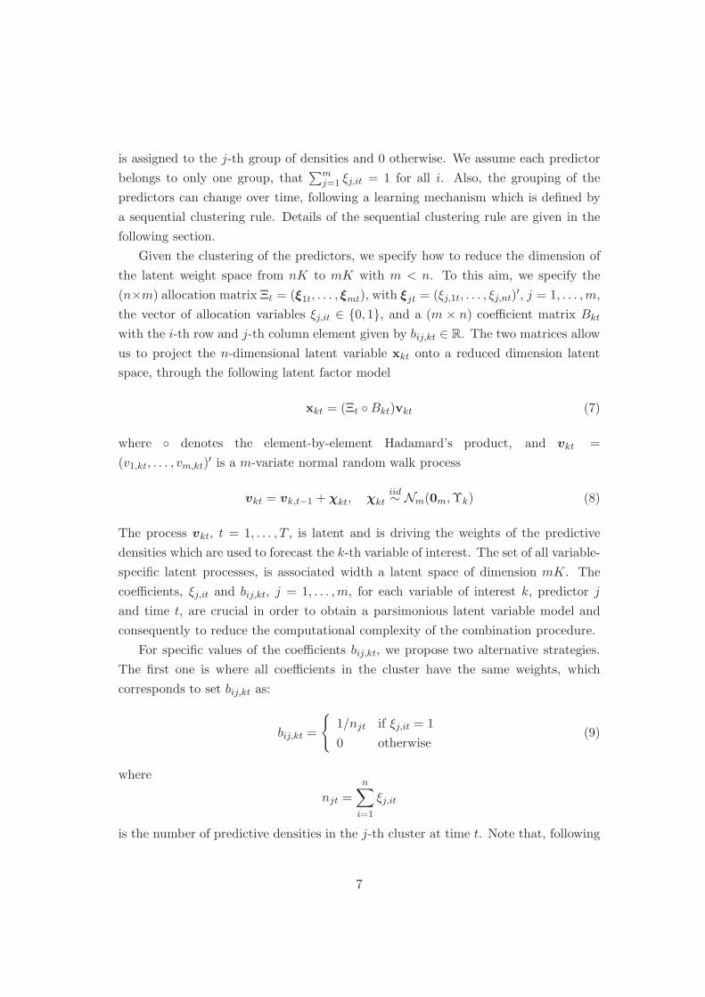
is assigned to the j-th group of densities and 0 otherwise. We assume each predictor

belongs to only one group, that∑m

j=1 ξj,it = 1 for all i. Also, the grouping of the

predictors can change over time, following a learning mechanism which is defined by

a sequential clustering rule. Details of the sequential clustering rule are given in the

following section.

Given the clustering of the predictors, we specify how to reduce the dimension of

the latent weight space from nK to mK with m < n. To this aim, we specify the

(n×m) allocation matrix Ξt = (ξ1t, . . . , ξmt), with ξjt = (ξj,1t, . . . , ξj,nt)′, j = 1, . . . ,m,

the vector of allocation variables ξj,it ∈ {0, 1}, and a (m × n) coefficient matrix Bkt

with the i-th row and j-th column element given by bij,kt ∈ R. The two matrices allow

us to project the n-dimensional latent variable xkt onto a reduced dimension latent

space, through the following latent factor model

xkt = (Ξt ◦Bkt)vkt (7)

where ◦ denotes the element-by-element Hadamard’s product, and vkt =

(v1,kt, . . . , vm,kt)′ is a m-variate normal random walk process

vkt = vk,t−1 +χkt, χktiid∼ Nm(0m,Υk) (8)

The process vkt, t = 1, . . . , T , is latent and is driving the weights of the predictive

densities which are used to forecast the k-th variable of interest. The set of all variable-

specific latent processes, is associated width a latent space of dimension mK. The

coefficients, ξj,it and bij,kt, j = 1, . . . ,m, for each variable of interest k, predictor j

and time t, are crucial in order to obtain a parsimonious latent variable model and

consequently to reduce the computational complexity of the combination procedure.

For specific values of the coefficients bij,kt, we propose two alternative strategies.

The first one is where all coefficients in the cluster have the same weights, which

corresponds to set bij,kt as:

bij,kt =

{

1/njt if ξj,it = 1

0 otherwise(9)

where

njt =

n∑

i=1

ξj,it

is the number of predictive densities in the j-th cluster at time t. Note that, following

7

this specification of the coefficients, the weights of the n predictors for the k-th variable

of interest are

wi,kt =exp{vji,kt/njit}

∑mj=1 exp{vj,kt/njt}

, i = 1, . . . , n

where ji =∑m

j=1 jξj,it indicates the group to which the i-th predictor belongs. The

latent weights are driven by a set of m latent variables, with m < n, thus the

dimensional reduction of the latent space is achieved. Moreover, let Nit = {j =

1, . . . , n|ξi,jt = 1} be the set of the indexes of all models in the cluster i, then one can

see that this specifications may have the undesirable property that the weights are

constant within a group, that is for all j ∈ Nit.

For this reason, we also propose the second specification strategy where we assume

that each model contributes to the combination with a specific weight that is driven

by a model-specific forecasting performance measure. If we assume git is the log score

(see definition in (B.43)) of the model i at time t then

bij,kt =

{

∑ts=1 exp{gis}/git if ξj,it = 1

0 otherwise(10)

where git =∑

l∈Nit

∑ts=1 exp{gls}.

All the modeling assumptions discussed above allow us to reduce the complexity

of the combination exercise because the set of time-varying combination weights to

estimate is of dimension mK < nK.

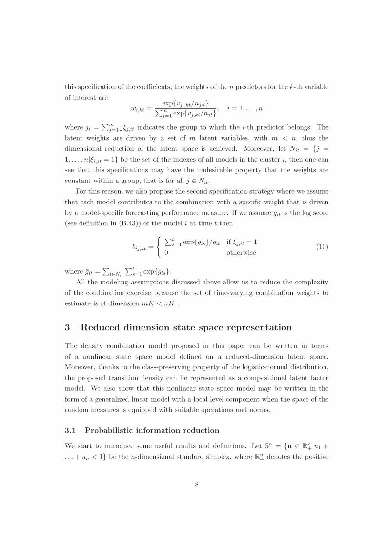
3 Reduced dimension state space representation

The density combination model proposed in this paper can be written in terms

of a nonlinear state space model defined on a reduced-dimension latent space.

Moreover, thanks to the class-preserving property of the logistic-normal distribution,

the proposed transition density can be represented as a compositional latent factor

model. We also show that this nonlinear state space model may be written in the

form of a generalized linear model with a local level component when the space of the

random measures is equipped with suitable operations and norms.

3.1 Probabilistic information reduction

We start to introduce some useful results and definitions. Let Sn = {u ∈ R

n+|u1 +

. . . + un < 1} be the n-dimensional standard simplex, where Rn+ denotes the positive

8

orthant of Rn. Proofs of results are presented in Appendix A.1.

Definition 3.1 (Composition function). The function Cm(u) : Rm+ → S

m−1, u 7→

v = Cm(u) with the i-the element of v defined as vi = ui/vm, i = 1, . . . ,m − 1, with

vm = u′ιm.

Proposition 3.1 (Logistic-normal distribution). Let v ∼ Nm (µ,Υ), and define

u = exp(v), that is the component-wise exponential transform of v, and z = Cm(u),

that is the composition of u, then u follows a m-variate log-normal distribution,

Λm(µ,Υ), and z follows a logistic-normal distribution Lm−1(Dmµ,DmΥD′m) with

density function

p(z|µ,Υ) = |2πDmΥD′m|−1/2

m−1∏

j=1

zj

−1

exp(

−1

2(log(z/zm)−Dmµ) (11)

(DmΥD′m)−1 (log(z/zm)−Dmµ)

′)

(12)

where z ∈ Sm−1, zm,kt = 1 − z′ιm−1, Dm = (Im−1,−ιm−1) and ιm−1 is the (m − 1)

unit vector.

Corollary 3.1. Let vkt ∼ Nm (vkt−1,Υk), and zkt = Cm(exp(vkt)), then zkt ∈ Sm−1

follows the logistic-normal distribution Lm−1(Dmvkt−1,DmΥkD′m).

The class-preserving property of the composition of the logistic-normal vectors (see

Aitchinson and Shen, 1980) will be used in the proof of the main result of this section.

We show how this property adapts to our state space model.

Proposition 3.2 (Class-preserving property). Let zkt ∼ Lm−1(Dmvkt−1,DmΥkD′m)

a logistic-normal vector, and A a (c×m− 1) matrix. Define the following transform

w = φA(z) from Sm−1 to S

c , with in our case m < c,

wi,kt =

m−1∏

j=1

(

zj,ktzm,kt

)aij

1 +

c∑

i=1

m−1∏

j=1

(

zj,ktzm,kt

)aij

−1

, i = 1, . . . , c

then wkt = (w1,kt, . . . , wc,kt) follows the logistic-normal Lc(ADmvkt−1, ADmΥkD′mA′).

3.2 A reduced dimension state space representation

Given the results in the preceding subsection, we can now state the main result.

9

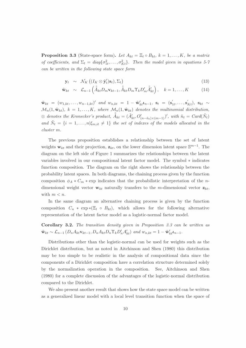
Proposition 3.3 (State-space form). Let Akt = Ξt ◦ Bkt, k = 1, . . . ,K, be a matrix

of coefficients, and Σt = diag{σ21t, . . . , σ

2Kt}. Then the model given in equations 5-7

can be written in the following state space form

yt ∼ NK

(

(IK ⊗ y′t)st),Σt

)

(13)

wkt ∼ Ln−1

(

˜AktDmvkt−1,˜AktDmΥkD

′m

˜A′kt

)

, k = 1, . . . ,K (14)

wkt = (w1,kt, . . . , wn−1,kt)′ and wn,kt = 1 − w′

ktιn−1, st = (s′

1t, . . . , s′

Kt), skt ∼

Mn(1, wkt), k = 1, . . . ,K, where Mn(1, wkt) denotes the multinomial distribution,

⊗ denotes the Kronecker’s product,˜Akt = (A′

kt, O′(n−nt)×(m−1))

′, with nt = Card(Nt)

and Nt = {i = 1, . . . , n|ξm,it 6= 1} the set of indexes of the models allocated in the

cluster m.

The previous proposition establishes a relationship between the set of latent

weights wkt and their projection, zkt, on the lower dimension latent space Sm−1. The

diagram on the left side of Figure 1 summarizes the relationships between the latent

variables involved in our compositional latent factor model. The symbol ∗ indicates

function composition. The diagram on the right shows the relationship between the

probability latent spaces. In both diagrams, the chaining process given by the function

composition φA ∗ Cm ∗ exp indicates that the probabilistic interpretation of the n-

dimensional weight vector wkt naturally transfers to the m-dimensional vector zkt,

with m < n.

In the same diagram an alternative chaining process is given by the function

composition Cn ∗ exp ∗(Ξt ◦ Bkt), which allows for the following alternative

representation of the latent factor model as a logistic-normal factor model.

Corollary 3.2. The transition density given in Proposition 3.3 can be written as

wkt ∼ Ln−1 (DnAktvkt−1,DnAktDnΥkD′nA

′kt) and wn,kt = 1− w′

ktιn−1.

Distributions other than the logistic-normal can be used for weights such as the

Dirichlet distribution, but as noted in Aitchinson and Shen (1980) this distribution

may be too simple to be realistic in the analysis of compositional data since the

components of a Dirichlet composition have a correlation structure determined solely

by the normalization operation in the composition. See, Aitchinson and Shen

(1980) for a complete discussion of the advantages of the logistic-normal distribution

compared to the Dirichlet.

We also present another result that shows how the state space model can be written

as a generalized linear model with a local level transition function when the space of

10

Figure 1: Relationships between the latent variables (left) and the latent probabilityspaces (right) involved in our compositional latent factor model. The origin of thedirected edge indicates the transformed variable, the arrow indicates the results ofthe transformation, and the edge label defines the transform applied. The symbol ∗indicates a composition of functions.

the random measures is equipped with suitable operations and norms. Moreover, we

show that the probabilistic interpretation is preserved for the lower dimensional set of

latent weights.

Define the observation real space RK equipped with the inner product < x,y >=

∑Ki=1 xiyi, x,y ∈ R

K and scalar product ax = (ax1, . . . , axK)′, x ∈ RK , a ∈ R

operations. Also, define the simplex (state) space, Sn−1 equipped with a sum operation

(also called perturbation operation), u⊕v = C(u◦v), u,v ∈ Sn−1 and a scalar product

operation (also called power transform) a⊙u = C((ua1, . . . , uan−1)

′), u ∈ Sn−1, a ∈ R+.

For details and background, see Aitchinson (1986) and Aitchinson (1992). Billheimer

et al. (2001) showed that Sn−1 equipped with the perturbation and powering operations

is a vector space. Moreover Sn−1 is an Hilbert space, i.e. a complete, inner product

vector space, equipped with the inner product < u,v >N= u,v ∈ Sn−1 space. These

properties enable us to state the following result.

Corollary 3.3. The state space model given in Proposition 3.3 can be written as

yt = (IK ⊗ y′t)st + εt, εt ∼ NK(0,Σt) (15)

wt = φ(zt) (16)

zkt = zkt−1 ⊕ ηkt, ηkt ∼ Lm−1

(

0,DnΥkD′m

)

(17)

where st = (s′

1t, . . . , s′

Kt) with skt ∼ Mn(1,wkt), k = 1, . . . ,K, is an allocation vector,

φ(zt) = (φA1t(z1t), . . . , φAKt

(zKt)) is a function from Sm−1 to S

n−1, where the function

φA(z) has been defined in 3.2.

11

The representation in corollary 3.3 shows that the model is a conditionally linear

model with link function defined by φA and a linear local level factor model on the

simplex. Also, by extending the ⊙ product operation to the case the external element

of the simplex is a matrix of real numbers and exploiting the Euclidean vector space

structure of (Sn,⊕,⊙) allow us to write the transform φA, for special values of A, as

a linear matrix operation between simplices of different dimension as stated in the

following remark. With a little abuse of notation we use the symbol ⊙ also for the

matrix multiplication operation.

Remark 1. Let z ∈ Sm−1 be a composition, A a (n × m) real matrix and define

the matrix multiplication A⊙ z = Cn

(

∏mj=1 z

a1jj , . . . ,

∏mj=1 z

an−1j

j

)

. If A is such that

Aιm = 0n and aim = −1, i = 1, . . . , n − 1 and an,j = 0 j = 1, . . . ,m, the transform

defined in proposition 3.2 can be written as φA(z) = A⊙ z.

A simulated example of compositional factor model is given in section B.1 of

the Online Appedix. We refer to the Billheimer et al. (2001) for further details on

the algebraic structure of the simplex equipped with the perturbation and powering

composition and for a Gibbs sampling scheme for compositional state space model. See

also Egozcue et al. (2003), Egozcue and Pawlowskky-Glahn (2005) and Fiserova (2011)

for further details on the isometric transforms from the real space to the simplex and

and for further geometric aspects and property analysis of operations on the simplex,

such as the amalgamation and subcomposition operations. See also Pawlowsky-Glahn

and Buccianti (2011) and Pawlowsky-Glahn et al. (2015) for up-to-date and complete

reviews on compositional data models.

4 Sequential inference

The analytical solution of the optimal filtering problem is generally not known, also the

clustering-based mapping of the predictor weights onto the subset of latent variables

requires the solution of an optimization problem which is not available in closed form.

Thus, we apply a sequential numerical approximation of the two problems and use an

algorithm which, at time t iterates over the following two steps:

1. Parallel sequential clustering computation of Ξt

2. Sequential Monte Carlo approximation of combination weights and predictive

densities

12

As regards the sequential clustering, we apply a parallel and sequential k-means

method with a forgetting factor for the sequential learning of the group structure.

K-means clustering, see for an early treatment Hartigan and Wong (1979), is a

method partitioning a set of n vectors of parameters or features of the predictors,

ψit, i = 1, . . . , n, into m disjoints sets (clusters), in which each observation belongs

to the cluster with the least distance. Moreover, the sequential k-means algorithm

is easy to parallelize and it has been done on multi core CPU and GPU computing

environments, see Rebolledo et al. (2008) and the reference therein. The details of the

algorithm and its parallel implementation are given in Appendix A.3.

As regards the sequential filtering we apply sequential Monte Carlo. The state-

form representations given in section 3 can be used to write the density combination in

terms of nonlinear sequential filtering and to apply the estimation strategy proposed

in Billio et al. (2013). Our approach contributes to the literature on time series on a

bounded domain (see, e.g., Aitchinson, 1982, Aitchinson, 1986, Wallis, 1987, Billheimer

et al., 2001 and Casarin et al., 2012) and on state space models for compositional data

analysis (see,e.g., Grunwald et al., 1993). In that literature the compositional data

are usually observed, while in our model the weights are latent probabilities.

Let θt ∈ Θ be the parameter vector of the combination model, that is θt =

(log σ21t, . . . , log σ

2Kt, vecd(Υ1t), . . . , vecd(ΥKt)). Let w

′t = (w′

1t, . . . ,wkt) the vector of

weights, and u1:t = (u1, . . . ,ut) the collection of vectors ut from time 1 to time t.

Following Kitagawa (1998), Kitagawa and Sato (2001), and Liu and West (2001), we

define the augmented state vector wθt = (wt,θt) ∈ Z, and the augmented state space

W = Sn−1 ×Θ. Our combination model writes in the state space form

yt ∼ p(yt|wθt , yt) (measurement density) (18)

wθt ∼ p(wθ

t |wθt−1,y1:t−1, y1:t−1) (transition density) (19)

wθ0 ∼ p(wθ

0) (initial density) (20)

where the measurement density is

p(yt|wθt , yt) ∝

K∏

k=1

fkt(ykt|wkt, σ2kt, yt) (21)

13

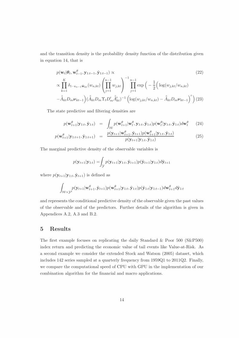
and the transition density is the probability density function of the distribution given

in equation 14, that is

p(wt|θt,wθt−1,y1:t−1, y1:t−1) ∝ (22)

∝K∏

k=1

δ1−ιn−1wkt(wn,kt)

n−1∏

j=1

wj,kt

−1n−1∏

j=1

exp(

−1

2

(

log(wj,kt/wn,kt)

− ˜AktDmνkt−1

)

( ˜AktDmΥtD′m˜A′kt)

−1(

log(wj,kt/wn,kt)−˜AktDmνkt−1

)′ )

(23)

The state predictive and filtering densities are

p(wθt+1|y1:t, y1:t) =

∫

W

p(wθt+1|w

θt ,y1:t, y1:t)p(w

θt |y1:t, y1:t)dw

θt (24)

p(wθt+1|y1:t+1, y1:t+1) =

p(yt+1|wθt+1, yt+1)p(w

θt+1|y1:t, y1:t)

p(yt+1|y1:t, y1:t)(25)

The marginal predictive density of the observable variables is

p(yt+1|y1:t) =

∫

Y

p(yt+1|y1:t, yt+1)p(yt+1|y1:t)dyt+1

where p(yt+1|y1:t, yt+1) is defined as

∫

W×Yt

p(yt+1|wθt+1, yt+1)p(w

θt+1|y1:t, y1:t)p(y1:t|y1:t−1)dw

θt+1dy1:t

and represents the conditional predictive density of the observable given the past values

of the observable and of the predictors. Further details of the algorithm is given in

Appendices A.2, A.3 and B.2.

5 Results

The first example focuses on replicating the daily Standard & Poor 500 (S&P500)

index return and predicting the economic value of tail events like Value-at-Risk. As

a second example we consider the extended Stock and Watson (2005) dataset, which

includes 142 series sampled at a quarterly frequency from 1959Q1 to 2011Q2. Finally,

we compare the computational speed of CPU with GPU in the implementation of our

combination algorithm for the financial and macro applications.

14

5.1 Predicting Standard & Poor 500 (S&P500)

The econometrician interested in predicting this index (or a transformation of it as

the return) has, at least, two standard strategies. First, she can model the index with

a parametric or non-parametric specification and produce a forecast of it. Second, she

can predict the price of each stock i and then aggregate them using an approximation

of the unknown weighting scheme.

We propose an alternative strategy based on the fact that many investors, including

mutual funds, hedge funds and exchange-traded funds, try to replicate the performance

of the index by holding a set of stocks, which are not necessarily the exact same stocks

included in the index. We collect 3712 individual stock daily prices quoted in the

NYSE and NASDAQ from Datastream over the sample March 18, 2002 to December

31, 2009, for a total of 2034 daily observation. To control for liquidity we impose that

each stock has been traded a number of days corresponding to at least 40% of the

sample size. We compute log returns for all stocks. Cross-section average statistics

are reported in Table 1, together with statistics for the S&P500. Some series have

much lower average returns than the index and volatility higher than the index up to

400 times. Heterogeneity in skewness is also very evident with the series with lowest

skewness equal to -42.5 and the one with highest skewness equal to 27.3 compared to

a value equal to -0.18 for the index. Finally, maximum kurtosis is 200 times higher

than the index value. The inclusion in our sample of the crisis period explains such

differences, with some stocks that realized enormously negative returns in 2008 and

impressive positive returns in 2009. We produce a density forecast for each of the stock

prices and then apply our density combination scheme to compute clustered weights

and a combined density forecast of the index. The output is a density forecast of the

index with clustered weights that indicate the relative forecasting importance of these

clusters. That is, a side output of our method is that it produces a replication strategy

of the index, providing evidence of which assets track more accurately the aggregate

index. We leave a detailed analysis of this last topic for further research.

Individual model estimates

We estimate a Normal GARCH(1,1) model and a t-GARCH(1,1) model via

maximum likelihood (ML) using rolling samples of 1250 trading days (about five years)

for each stock return:

yit = ci + κitζit (26)

κ2it = θi0 + θi1ζ2i,t−1 + θ2κ

2i,t−1 (27)

15

Subcomponents S&P500

Lower Median UpperAverage -0.002 0.000 0.001 0.000St dev 0.016 0.035 0.139 0.019Skewness -1.185 0.033 1.060 -0.175Kurtosis 8.558 16.327 65.380 9.410Min -1.322 -0.286 -0.121 -0.095Max 0.122 0.264 1.386 0.110

Table 1: Average cross-section statistics for the 3712 individual stock daily log returns inour dataset for the sample 18 March 2002 to 31 December 2009. The columns “Lower”,“Median” and “Upper” refer to the cross-section 10% lower quantile, median and 90% upperquantile of the 3712 statistics in rows, respectively. The rows “Average”, “St dev”, “Skewness”,“Kurtosis”, “Min” and “Max” refers to sample average, sample standard deviation, sampleskewness, sample kurtosis, sample minimum and sample maximum statistics, respectively. Thecolumn “S&P500” reports the sample statistics for the aggregate S&P500 log returns.

where yit is the log return of stock i at day t, ζit ∼ N (0, 1) and ζit ∼ T (νi) for the

Normal and t-Student cases, respectively. The number of degrees of freedom νi is

estimated in the latter model. We produce 784 one day ahead density forecasts from

January 1, 2007 to December 31, 2009 using the above equations and the first day

ahead forecast refers to January 1, 2007. Our out-of-sample (OOS) period is associated

with high volatility driven by the US financial crisis and includes, among others, events

such as the acquisitions of Bern Stearns, the default of Lehman Brothers and all the

following week events. The predictive densities are formed by substituting the ML

estimates for the unknown parameters (ci, θi0, θi1, θi2, νi). We also collect the S&P500

index from Datastream over the same sample.

As first step, we apply a sequential cluster analysis to our forecasts. We compute

two clusters for the Normal GARCH(1,1) model class and two clusters for the t-

GARCH(1,1) model class. The first two are characterized by low and high volatility

density predictions from Normal GARCH(1,1) models; the third and the fourth ones

are characterized by thick or no thick tail density predictions from t-GARCH(1,1)

models.3

Figure 2 presents the mean values of the predicted features ψit which belong to the

j−th cluster at each of the 784 vintages, labeled as mjt+1. The clusters for the Normal

GARCH(1,1) models differ substantially in terms of predicted variance with cluster

1 having a rather low constant variance value over the entire period while cluster 2

3Low degrees of freedom occur jointly with a large scale and high degrees of freedom occur jointlywith a low scale.

16

20070101 20080101 20090101 200912310.05

0.1

0.15

0.2

0.25

0.3

0.35

0.4

12

20070101 20080101 20090101 200912310

5

10

15

20

25

30

34

Normal GARCH(1,1) t-GARCH(1,1)

Figure 2: The figures present the average variance of the predictions from the two clustersfor the Normal GARCH(1,1) models based on low (cluster 1) and high (cluster 2) volatility inthe left panel; and the average degree of freedom of the predictions from the two clusters forthe t-GARCH(1,1) models based on low (cluster 3) and high (cluster 4) degrees of freedom inthe right panel. The degrees of freedom are bounded to 30.

has a variance more than double in size including a shock in the latter part of 2008.

For the t-GARCH(1,1) model it is seen that cluster 3 has a relatively constant thick

tail over the entire period while cluster 4 has an average value of 10 for the degrees

of freedom and in the crisis period the density collapses to a normal density with

degrees of freedom higher than 30. In summary, The Lehman Brother effect is visible

in the figure, with an increase of volatility in the normal cluster 2 and, interesting, an

increase of the degrees of freedom in the t-cluster 4.

Weight patterns, model incompleteness and signals of instability

For convenience, we specified the parameter matrices Bkt in equation (9), the

cluster weights, as equal weights.4 We also allow for model incompleteness to be

modeled as a time-varying process and estimate σ2kt in (5). We label it DCEW-SV

and compare it with a combination scheme where σ2kt = σ2

k is time-invariant and label

that as DCEW. We compare our two combination methods, DCEW and DCEW-SV

described in section 5.1 to the standard no predictability white noise benchmark and

also apply the Normal GARCH(1,1) model and the t-Student GARCH(1,1) model

to the index log returns. The comparison is done by applying the predictive ability

measures defined in Appendix B.3.

Plots of the time patterns of the weights of the 4 clusters are shown in Figure

3 (left panel). These are the logistic-normal weights zk,t defined in Corollary 3.1.

4See the macroeconomic case below for a comparison with a different scoring rule.

17

20070101 20080101 20090101 200912310

0.2

0.4

0.6

0.8

1

Norm1 Norm2 t1 t2

20070101 20080101 20090101 200912310.99

1

1.01

1.02

1.03

1.04

1.05

1.06

1.07

1.08

1.09x 10

−4

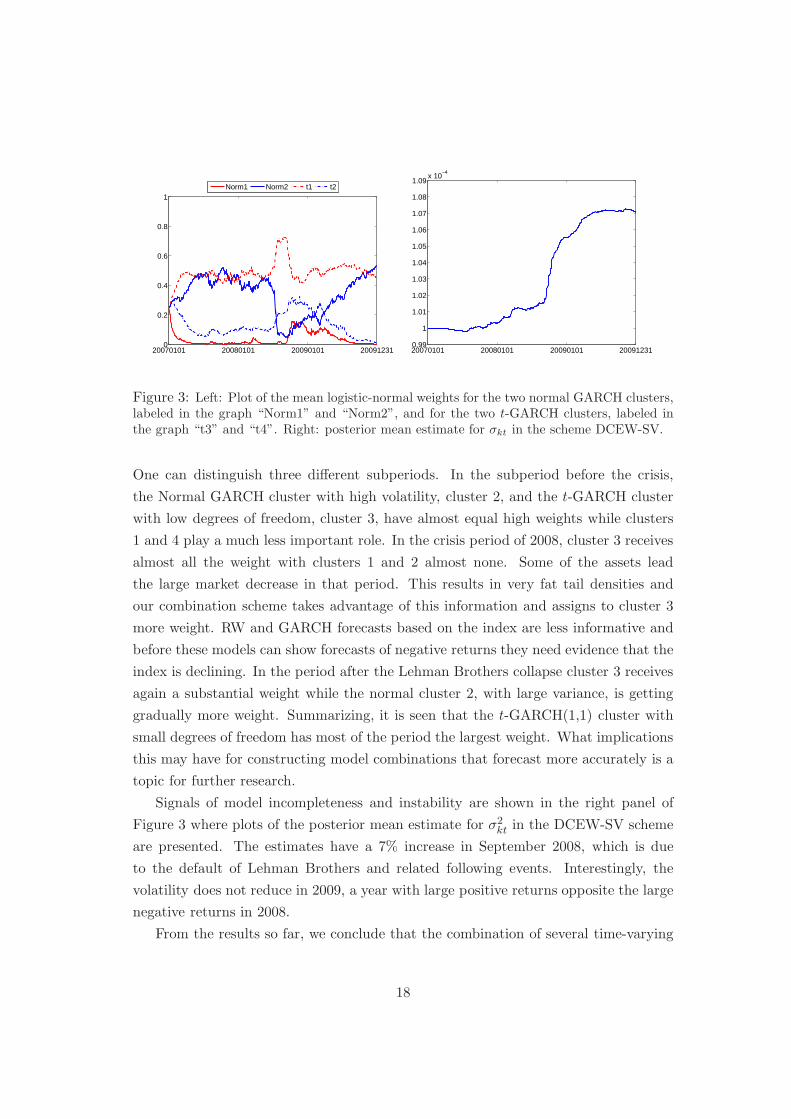
Figure 3: Left: Plot of the mean logistic-normal weights for the two normal GARCH clusters,labeled in the graph “Norm1” and “Norm2”, and for the two t-GARCH clusters, labeled inthe graph “t3” and “t4”. Right: posterior mean estimate for σkt in the scheme DCEW-SV.

One can distinguish three different subperiods. In the subperiod before the crisis,

the Normal GARCH cluster with high volatility, cluster 2, and the t-GARCH cluster

with low degrees of freedom, cluster 3, have almost equal high weights while clusters

1 and 4 play a much less important role. In the crisis period of 2008, cluster 3 receives

almost all the weight with clusters 1 and 2 almost none. Some of the assets lead

the large market decrease in that period. This results in very fat tail densities and

our combination scheme takes advantage of this information and assigns to cluster 3

more weight. RW and GARCH forecasts based on the index are less informative and

before these models can show forecasts of negative returns they need evidence that the

index is declining. In the period after the Lehman Brothers collapse cluster 3 receives

again a substantial weight while the normal cluster 2, with large variance, is getting

gradually more weight. Summarizing, it is seen that the t-GARCH(1,1) cluster with

small degrees of freedom has most of the period the largest weight. What implications

this may have for constructing model combinations that forecast more accurately is a

topic for further research.

Signals of model incompleteness and instability are shown in the right panel of

Figure 3 where plots of the posterior mean estimate for σ2kt in the DCEW-SV scheme

are presented. The estimates have a 7% increase in September 2008, which is due

to the default of Lehman Brothers and related following events. Interestingly, the

volatility does not reduce in 2009, a year with large positive returns opposite the large

negative returns in 2008.

From the results so far, we conclude that the combination of several time-varying

18

volatility models with time-varying cluster weights copes with instability in our set

of data. There is a clear signal of increased model incompleteness after the 2008

crisis. Individual flexible models that focus more on jumps in volatility and use data

on realized volatility may be included in the analysis. This is an interesting topic of

further research.

Forecast accuracy and economic value

Out-of-sample forecasting result are presented in Table 2. Our combination

schemes produce the lowest RMSPE and CRPS and the highest LS. The results

indicate that the combination schemes are statistically superior to the no predictability

benchmark. The Normal GARCH(1,1) model and t-GARCH(1,1) model fitted on the

index also provide more accurate density forecasts than the WN, but not on point

forecasting. For all three score criteria, the statistics given by the two individual

models are inferior to our combination schemes. Therefore, we conclude that our

strategy to produce forecasts from a large set of assets, cluster them in groups

and combine them to predict the S&P500 produces very accurate point and density

forecasts that are superior to no predictability benchmark and classical strategies of

modeling directly the index.

Apart from forecasting accuracy, we investigate whether the results documented in

the previous paragraphs also possess some economic value. Given that our approach

produces complete predictive densities for the variable of interest, it is particularly

suitable to compute tail events and, therefore, Value-at-Risk (VaR) measures, see

Jorion (2000). We compare the accuracy of our models in terms of violations, that is

the number of times that negative returns exceed the VaR forecast at time t, with the

implication that actual losses on a portfolio are worse than had been predicted. Higher

accuracy results in numbers of violation close to nominal value of 1%. Moreover, to

have a gauge of the severity of the violations we compute the total losses by summing

the returns over the days of violation for each model.

The last two columns of 2 show that the number of violations for all models is

high and well above 1%, with the RW higher than 20%. The dramatic events in our

sample, including the Lehman default and all the other features of the US financial

crisis, explain the result. However, the two combination schemes provide the best

statistics, with violations almost 50% lower than the best individual model and losses

at least 15% lower than the best individual models. The DCEW-SV provides the

most accurate results, but the difference with DCEW is marginal. The property of

our combination schemes to assign higher weights to the fat tail cluster 3 helps to

model more accurately the lower tail of the index returns and covers more adequately

19

risks.

Finally, Table B.5 in Appendix B.5 compares the execution time of the GPU

parallel implementation of our density combination strategy and the CPU multi-core

implementation and show large gains from GPU parallelization.

RMSPE LS CRPS Violation Loss

WN 1.8524 -9.0497 0.0102 20.3% -50.1%Normal GARCH 1.8522 -4.1636∗∗ 0.0096∗∗ 16.5% -42.2%t-GARCH 1.8524 -2.7383∗∗ 0.0094∗∗ 11.4% -32.9%DCEW 1.8122∗∗ 2.2490∗∗ 0.0091∗∗ 6.6% -28.1%DCEW-SV 1.8165∗∗ 2.2060∗∗ 0.0091∗∗ 6.5% -27.7%

Table 2: Forecasting results for next day S&P500 log returns. For all the series arereported the: root mean square prediction error (RMSPE), logarithmic score (LS) and thecontinuous rank probability score (CRPS). Bold numbers indicate the best statistic for eachloss function. One or two asterisks indicate that differences in accuracy from the white noise(WN) benchmark are statistically different from zero at 5%, and 1%, respectively, using theDiebold-Mariano t-statistic for equal loss. The underlying p-values are based on t-statisticscomputed with a serial correlation-robust variance, using the pre-whitened quadratic spectralestimator of Andrews and Monahan (1992). The column “Violation” shows the number oftimes the realized value exceeds the 1% Value-at-Risk (VaR) predicted by the different modelsover the sample and the column “Loss” reports the cumulative total loss associated to theviolations.

5.2 A large macroeconomic dataset

As a second example, we consider the extended Stock and Watson (2005) dataset,

which includes 142 series sampled at a quarterly frequency from 1959Q1 to 2011Q2.

A graphical description of the data is given in Figure B.2, in section B.4 of the Online

Appendix. The dataset includes only revised series and not vintages of real-time data,

when data are revised. See Aastveit et al. (2014) for a real-time application (with

a dataset that includes fewer series) of density nowcasting and on the role of model

incompleteness over vintages and time. In order to deal with stationary series, we

apply the series-specific transformation suggested in Stock and Watson (2005). Let

yit with i = 1, . . . , n and t = 1, . . . , T , be the set of transformed variables.

For each variable we estimate a Gaussian autoregressive model of the first order,

AR(1),

yit = αi + βiyit−1 + ζit, ζit ∼ N (0, σ2i ) (28)

using the first 60 observations from each series. Then we identify the clusters

of parameters by applying our k-means clustering algorithm on the vectors, θi =

20

(αi, βi, σ2i )

′, of least square estimates of the AR(1) parameters. Since we are interested

in an interpretation of the clusters over the full sample, differently than in the previous

financial application, we impose that cluster allocation of each model is fixed over the

forecasting vintages, i.e. Ξt = Ξ, t = 1, . . . , T . The first 102 observations, from

1959Q3 to 1984Q1, are used as initial in-sample (IS) period to fit AR(1) models to

all the individual series and construct the clusters. We assume alternatively 5 and 7

clusters. A detailed description of the 7 clusters is provided in Table B.3 in section

B.4 of the Online Appendix, together with further results.

Set-up of the experiment

We split the sample size 1959Q3-2011Q2 in two periods. The initial 102

observations from 1959Q3-1984Q1 are used as initial in-sample (IS) period; the

remaining 106 observations from 1985Q1-2011Q2 are used as an OOS period. The AR

models are estimated recursively and h−step ahead (Bayesian) t−Student predictive

densities are constructed using a direct approach extending each vintage with the new

available observation; see for example Koop (2003) for the exact formula of the mean,

standard deviation and degrees of freedom. Clusters are, however, not updated and

kept the same as the ones estimated in the IS period.

We predict four different series often considered core variables in monetary policy

analysis: real GDP growth, inflation measured as price deflator growth, 3-month

Treasury Bill rate and total employment. We consider h = 1, 2, 3, 4, 5 step-ahead

horizons. For all the variables to be predicted, we apply an AR(1) as benchmark

model.

Our methodology allows for considerable flexibility and several combination

schemes can be derived. As we described in Section 2, we consider two alternative

strategies for the specification of the parameter matrices Bkt: equal weights and

score recursive weights, where in the second case we fix gi = LSi,h for the various

horizons h presented in the following subsection. Further, the predictive densities

given by equation (B.39) can be combined with each of the four univariate series and/or

with a multivariate approach. Following the evidence in Appendix B.4 we apply two

clusters, k = 5 and 7. We note that we keep the volatility of the incompleteness term

constant. To sum up, we have eight cases defined as UDCEW5 (univariate combination

based on 5 clusters with equal weights within clusters), MDCEW5 (multivariate

combination based on 5 clusters with equal weights within clusters), UDCLS5

(univariate combination based on 5 clusters with recursive log score weights within

clusters), MDCLS5 (multivariate combination based on 5 clusters with recursive log

score weights within clusters), UDCEW7 (univariate combination based on 7 clusters

21

with equal weights within clusters), MDCEW7 (multivariate combination based on 7

clusters with equal weights within clusters), UDCLS7 (univariate combination based

on 7 clusters with recursive log score weights within clusters), MDCLS7 (multivariate

combination based on 7 cluster with recursive log score weights within clusters).

Apart from the AR(1) benchmark we also compare our combinations to a

benchmark that is specified as Dynamic Factor Model (DFM) with 5 factors described

in Stock and Watson (2012). This DFM expresses each of the n time series as

a component driven by the latent factors plus ad idiosyncratic disturbance. More

precisely:

Yt = ΛFt +Σt, Φ(L)Ft = ηt, (29)

where the Yt = {y1,t, . . . , yn,t} is an n×1 vector of observed series, Ft = {f1,t, . . . , fr,t}

is an r × 1 vector of latent factors, Λ is a n× r matrix of factors loadings, Φ(L) is an

r × r matrix lag polynomial, Σt = {ε1,t, . . . , εn,t} is an n × 1 vector of idiosyncratic

components and ηt is an r × 1 vector of innovations. In this formulation the term

ΛFt is the common component of Yt. Bayesian estimation of the model described in

equation (29) is carried out using Gibbs Sampling given in Koop and Korobilis (2009).

Weight patterns and forecasting results

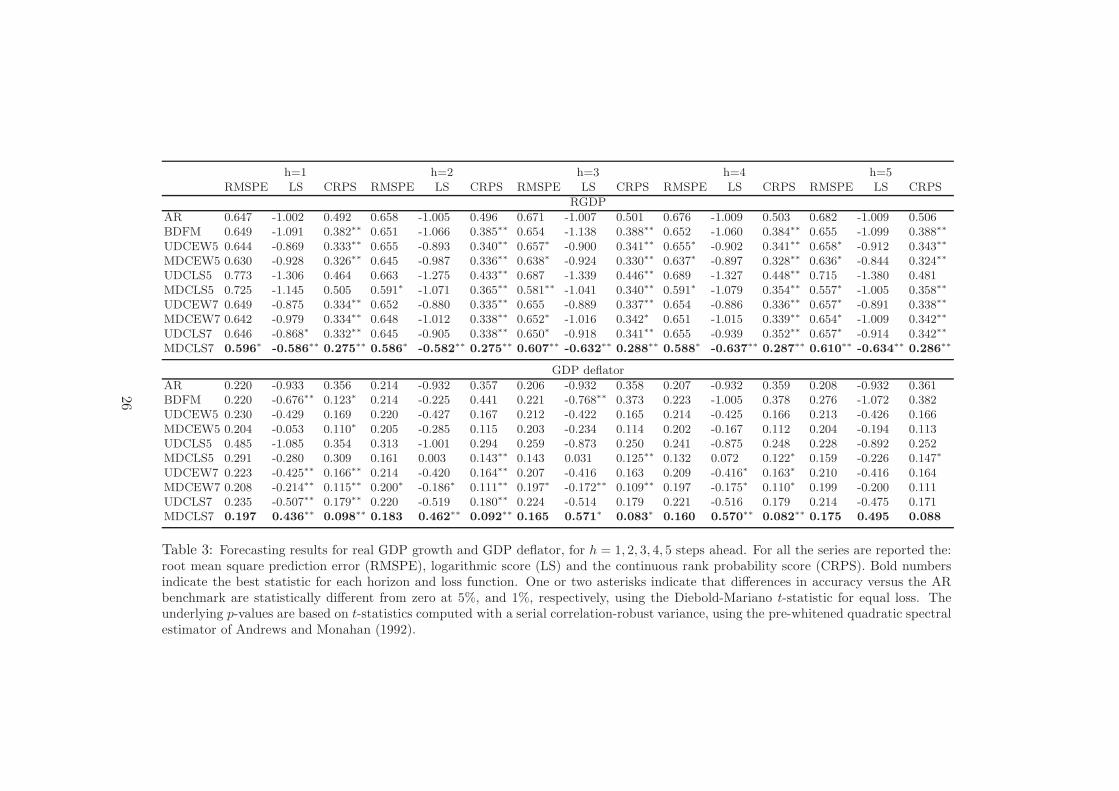
Tables 3-4 report the results to predict real GDP growth, inflation measured by

using the price deflator of GDP growth, 3-month Treasury Bills and total employment

for five different horizons and using three different scoring measures. For all variables,

horizons and scoring measures our methodology provides more accurate forecasts than

the AR(1) benchmark and the Bayesian DFM. The Bayesian DFM model provides

more accurate forecasts than the AR(1) for real GDP and inflation at shorter horizons

and gives mixed evidence for interest rates and unemployment, but several of our

combination schemes outperform this benchmark. The combination that provides the

largest gain is the multivariate one based on seven clusters and log score weights

within clusters (MCDLS7), resulting in the best statistics 56 times over 60. In most of

the cases, the difference is statistically credible at the 1% level. This finding extends

evidence on the scope for multi-variable forecasting such as in large Bayesian VAR, see

e.g. Banbura et al. (2010) and Koop and Korobilis (2013). Fan charts in Figure B.7 in

the Appendix B.4 show that the predictions are accurate even at our longest horizon,

h = 55. The variable with low predictive gains is inflation, although our method

provides credibly more accurate scores at (at least) 5% credible level in 8 cases over

15, but none in terms of point forecasting. The multivariate combination based on

5 clusters and equal weights yields accurate forecasts, see clusters (MCDEW5). We

22

conclude that combining models using multiple clusters with cluster-based weights

provides substantial forecast gains in most cases. Additional gains may be obtained

by playing with a more detailed cluster grouping and different performance scoring

rules for weights associated with models inside a cluster.

Figure 4 show the time pattern of the weights in the seven clusters for each of the

variables to be predicted and a selection of horizons, h = 1, 2, 5, using multivariate

combinations and assuming bk,ij equal to the recursive log score for model i in cluster

j when predicting the series k (see Figure B.5 in Appendix B.4 for weights in the

univariate combination. We notice that the weights for the univariate are often less

volatile than the weights in the multivariate approach). We plot the logistic-normal

weights zk,t defined in Corollary 3.1. In both figures, the sixth cluster receives the

largest weight for all variables, but several other clusters have large positive weights,

like clusters 2, 4, and 5 while clusters 1 and 7 do not receive much weight. Apparently,

variables such as Exports, Imports and GDP deflator included in the sixth cluster play

an important role in forecasting GDP growth, inflation, interest rate and employment,

although this role may differ across variables and horizons.

The forecast gains are similar across horizons for the five variables, that is around

10% relative to the AR benchmark in terms of RMSPE metrics and even larger

for the log score and CRPS measures. The lowest improvements are evident when

predicting the 3-month Treasury Bills. Despite these consistent gains over horizons,

the combination weights in Figure 4 differ across horizons. For example, when

forecasting GDP growth (panel 1) cluster 4 has a weight around 20% at horizons

1 and 5, but half of this value at horizon 3, where clusters 2 and 5 have larger weights.

The change is even more clear for inflation, where cluster 2 has a 20% weight at

horizon 1 and increases to 40-45% at horizon 5. The latter case also occurs when

there is substantial instability over time. Changes over horizons are less relevant for

the other two predicted variables.

Figure B.6 in the Online Appendix shows a typical output of the model weights

(bk,ij) in the seven clusters. There are large differences across clusters: the clusters

2, 4, 5 and 6 have few models with most of the weights; the other clusters, 1, 3 and

7, have more similar weights across models. This finding should be associated with

the largest weights in Figure 4 for the clusters 2, 4, 5 and 6 and indicates that using

recursive time-varying bk,ij weights within the clusters increases forecast accuracy for

GDP growth relative to using equal weights. Figure B.6 also indicates that the weights

within clusters are much more volatile than the cluster common component, indicating

that individual model performances may change much over time even if information

23

1985Q1 1995Q1 2005Q1 2011Q20

0.1

0.2

0.3

0.4

0.5

0.6

0.7

w11t

w12t

w13t

w14t

w15t

w16t

w17t

1985Q1 1995Q1 2005Q1 2011Q20

0.1

0.2

0.3

0.4

0.5

w11t

w12t

w13t

w14t

w15t

w16t

w17t

1985Q1 1995Q1 2005Q1 2011Q20

0.1

0.2

0.3

0.4

0.5

w11t

w12t

w13t

w14t

w15t

w16t

w17t

1985Q1 1995Q1 2005Q1 2011Q20

0.1

0.2

0.3

0.4

0.5

w21t

w22t

w23t

w24t

w25t

w26t

w27t

1985Q1 1995Q1 2005Q1 2011Q20

0.1

0.2

0.3

0.4

0.5

w21t

w22t

w23t

w24t

w25t

w26t

w27t

1985Q1 1995Q1 2005Q1 2011Q20

0.1

0.2

0.3

0.4

0.5

0.6

0.7

w21t

w22t

w23t

w24t

w25t

w26t

w27t

1985Q1 1995Q1 2005Q1 2011Q20

0.1

0.2

0.3

0.4

0.5

w31t

w32t

w33t

w34t

w35t

w36t

w37t

1985Q1 1995Q1 2005Q1 2011Q20

0.1

0.2

0.3

0.4

0.5

w31t

w32t

w33t

w34t

w35t

w36t

w37t

1985Q1 1995Q1 2005Q1 2011Q20

0.1

0.2

0.3

0.4

0.5

w31t

w32t

w33t

w34t

w35t

w36t

w37t

1985Q1 1995Q1 2005Q1 2011Q20

0.1

0.2

0.3

0.4

0.5

w41t

w42t

w43t

w44t

w45t

w46t

w47t

1985Q1 1995Q1 2005Q1 2011Q20

0.1

0.2

0.3

0.4

0.5

w41t

w42t

w43t

w44t

w45t

w46t

w47t

1985Q1 1995Q1 2005Q1 2011Q20

0.1

0.2

0.3

0.4

0.5

0.6

0.7

w41t

w42t

w43t

w44t

w45t

w46t

w47t

Figure 4: In each plot the logistic-normal weights (different lines) for the multivariatecombination model are given. Rows: plot for the four series of interest (real GDP growthrate, GDP deflator, Treasury Bills, employment). Columns: forecast horizons (1, 3 and 5quarters).

24

in a given clusters is stable.

Evidence is similar for the GDP deflator and employment, but this finding is less

clear for bond returns. For this variable, MDCEW5 also predicts accurately. Also

notice that cluster 3, which includes the 3-month Treasury Bills, has the lowest weight

in Figures 4. The explanation appears to be that the returns on the 3-month Treasury

Bills are modeled with an AR model, which is probably less accurate for the series.

Furthermore, the third cluster also contains stock prices and exchange rates that are

different from other series with very low persistence and high volatility, making our

combination to interpret this cluster more like a noisy component.

We conclude that the cluster-based weights contain relevant signals about the

importance of the forecasting performance of each of the models used in the these

clusters. Some clusters have a substantial weight while others have only little weight

and such a pattern may vary over long time periods. This may lead to the construction

of alternative model combinations for more accurate out-of-sample forecasting and is

an interesting line of research to pursue.

6 Conclusions

We proposed in this paper a Bayesian nonparametric model to construct a time-varying

weighted combination of many predictive densities that can deal with large data sets in

economics and finance. The model is based on clustering the set of predictive densities

in mutually exclusive subsets and on a hierarchical specification of the combination

weights. This modeling strategy reduces the dimension of the parameter and latent

spaces and leads to a more parsimonious combination model. We provide several

theoretical properties of the weights and propose the implementation of efficient and

fast parallel clustering and sequential combination algorithms.

We applied the methodology to large financial and macro data sets and find

substantial gains in point and density forecasting for stock returns and four key macro

variables. In the financial applications, we show how 7000 predictive densities based

on US individual stocks can be combined to replicate the daily Standard & Poor 500

(S&P500) index return and predict the economic value of tail events like Value-at-

Risk. In the macroeconomic exercise, we show that combining models for multiple

series with cluster-based weights increases forecast accuracy substantially; weights

across clusters are very stable over time and horizons, with an important exception

for inflation at longer horizons. Furthermore, weights within clusters are very volatile,

indicating that individual model performances are very unstable, strengthening the

25

h=1 h=2 h=3 h=4 h=5RMSPE LS CRPS RMSPE LS CRPS RMSPE LS CRPS RMSPE LS CRPS RMSPE LS CRPS

RGDP

AR 0.647 -1.002 0.492 0.658 -1.005 0.496 0.671 -1.007 0.501 0.676 -1.009 0.503 0.682 -1.009 0.506BDFM 0.649 -1.091 0.382∗∗ 0.651 -1.066 0.385∗∗ 0.654 -1.138 0.388∗∗ 0.652 -1.060 0.384∗∗ 0.655 -1.099 0.388∗∗

UDCEW5 0.644 -0.869 0.333∗∗ 0.655 -0.893 0.340∗∗ 0.657∗ -0.900 0.341∗∗ 0.655∗ -0.902 0.341∗∗ 0.658∗ -0.912 0.343∗∗

MDCEW5 0.630 -0.928 0.326∗∗ 0.645 -0.987 0.336∗∗ 0.638∗ -0.924 0.330∗∗ 0.637∗ -0.897 0.328∗∗ 0.636∗ -0.844 0.324∗∗

UDCLS5 0.773 -1.306 0.464 0.663 -1.275 0.433∗∗ 0.687 -1.339 0.446∗∗ 0.689 -1.327 0.448∗∗ 0.715 -1.380 0.481MDCLS5 0.725 -1.145 0.505 0.591∗ -1.071 0.365∗∗ 0.581∗∗ -1.041 0.340∗∗ 0.591∗ -1.079 0.354∗∗ 0.557∗ -1.005 0.358∗∗

UDCEW7 0.649 -0.875 0.334∗∗ 0.652 -0.880 0.335∗∗ 0.655 -0.889 0.337∗∗ 0.654 -0.886 0.336∗∗ 0.657∗ -0.891 0.338∗∗

MDCEW7 0.642 -0.979 0.334∗∗ 0.648 -1.012 0.338∗∗ 0.652∗ -1.016 0.342∗ 0.651 -1.015 0.339∗∗ 0.654∗ -1.009 0.342∗∗

UDCLS7 0.646 -0.868∗ 0.332∗∗ 0.645 -0.905 0.338∗∗ 0.650∗ -0.918 0.341∗∗ 0.655 -0.939 0.352∗∗ 0.657∗ -0.914 0.342∗∗

MDCLS7 0.596∗

-0.586∗∗

0.275∗∗

0.586∗

-0.582∗∗

0.275∗∗

0.607∗∗

-0.632∗∗

0.288∗∗

0.588∗

-0.637∗∗

0.287∗∗

0.610∗∗

-0.634∗∗

0.286∗∗

GDP deflator

AR 0.220 -0.933 0.356 0.214 -0.932 0.357 0.206 -0.932 0.358 0.207 -0.932 0.359 0.208 -0.932 0.361BDFM 0.220 -0.676∗∗ 0.123∗ 0.214 -0.225 0.441 0.221 -0.768∗∗ 0.373 0.223 -1.005 0.378 0.276 -1.072 0.382UDCEW5 0.230 -0.429 0.169 0.220 -0.427 0.167 0.212 -0.422 0.165 0.214 -0.425 0.166 0.213 -0.426 0.166MDCEW5 0.204 -0.053 0.110∗ 0.205 -0.285 0.115 0.203 -0.234 0.114 0.202 -0.167 0.112 0.204 -0.194 0.113UDCLS5 0.485 -1.085 0.354 0.313 -1.001 0.294 0.259 -0.873 0.250 0.241 -0.875 0.248 0.228 -0.892 0.252MDCLS5 0.291 -0.280 0.309 0.161 0.003 0.143∗∗ 0.143 0.031 0.125∗∗ 0.132 0.072 0.122∗ 0.159 -0.226 0.147∗

UDCEW7 0.223 -0.425∗∗ 0.166∗∗ 0.214 -0.420 0.164∗∗ 0.207 -0.416 0.163 0.209 -0.416∗ 0.163∗ 0.210 -0.416 0.164MDCEW7 0.208 -0.214∗∗ 0.115∗∗ 0.200∗ -0.186∗ 0.111∗∗ 0.197∗ -0.172∗∗ 0.109∗∗ 0.197 -0.175∗ 0.110∗ 0.199 -0.200 0.111UDCLS7 0.235 -0.507∗∗ 0.179∗∗ 0.220 -0.519 0.180∗∗ 0.224 -0.514 0.179 0.221 -0.516 0.179 0.214 -0.475 0.171MDCLS7 0.197 0.436

∗∗0.098

∗∗0.183 0.462

∗∗0.092

∗∗0.165 0.571

∗0.083

∗0.160 0.570

∗∗0.082

∗∗0.175 0.495 0.088

Table 3: Forecasting results for real GDP growth and GDP deflator, for h = 1, 2, 3, 4, 5 steps ahead. For all the series are reported the:root mean square prediction error (RMSPE), logarithmic score (LS) and the continuous rank probability score (CRPS). Bold numbersindicate the best statistic for each horizon and loss function. One or two asterisks indicate that differences in accuracy versus the ARbenchmark are statistically different from zero at 5%, and 1%, respectively, using the Diebold-Mariano t-statistic for equal loss. Theunderlying p-values are based on t-statistics computed with a serial correlation-robust variance, using the pre-whitened quadratic spectralestimator of Andrews and Monahan (1992).

26

h=1 h=2 h=3 h=4 h=5RMSPE LS CRPS RMSPE LS CRPS RMSPE LS CRPS RMSPE LS CRPS RMSPE LS CRPS

3-month Treasury Bills

AR 0.569 -1.058 0.363 0.605 -1.074 0.374 0.518 -1.038 0.343 0.530 -1.037 0.353 0.545 -1.041 0.358BDFM 0.522∗ -1.190 0.359 0.694 -1.394 0.386 0.545 -1.092 0.392 0.552 -1.092 0.396 0.541 -1.089 0.401UDCEW5 0.519 -0.778∗∗ 0.288∗∗ 0.521 -0.782∗∗ 0.288 0.509 -0.772∗∗ 0.283 0.517 -0.782∗∗ 0.288∗ 0.525 -0.791∗∗ 0.292∗

MDCEW5 0.517∗∗ -0.764∗∗ 0.285∗∗ 0.506 -0.752∗∗ 0.279∗∗ 0.502∗ -0.749∗∗

0.276∗∗

0.506∗∗

-0.755∗∗

0.278∗∗ 0.505∗∗ -0.751∗∗ 0.278∗∗

UDCLS5 0.740 -1.254 0.448 0.678 -1.301 0.453 0.532 -1.210 0.381 0.528 -1.216 0.385 0.584 -1.286 0.424MDCLS5 0.710 -1.322 0.491 0.688 -1.297 0.454 0.491∗∗ -1.143 0.346 0.487 -1.143 0.351 0.572∗∗ -1.196 0.378UDCEW7 0.525 -0.783∗∗ 0.289∗ 0.526 -0.784∗∗ 0.289∗ 0.514 -0.768∗∗ 0.284∗ 0.518 -0.774∗∗ 0.286∗ 0.522 -0.786∗∗ 0.289∗

MDCEW7 0.526 -0.775∗∗ 0.289∗ 0.527 -0.777∗∗ 0.290∗ 0.515 -0.761∗∗ 0.283∗ 0.516 -0.765∗∗ 0.284∗ 0.513 -0.766∗∗ 0.283∗

UDCLS7 0.512 -0.773∗∗ 0.284∗ 0.521 -0.799∗∗ 0.291∗ 0.514 -0.770∗∗ 0.284∗ 0.519 -0.783∗∗ 0.286∗ 0.521 -0.793∗∗ 0.289∗

MDCLS7 0.488∗∗

-0.725∗∗

0.270∗∗

0.484∗∗

-0.771∗∗

0.275∗

0.515∗∗ -0.755∗∗ 0.283 0.513∗∗ -0.771∗∗ 0.283 0.496

∗∗-0.736

∗∗0.275

∗∗

Employment

AR 0.564 -0.995 0.447 0.582 -0.999 0.454 0.597 -1.003 0.460 0.612 -1.007 0.464 0.622 -1.009 0.468BDFM 0.571 -1.064 0.339∗∗ 0.565 -1.057 0.614 0.956 -1.192 0.907 0.724 -1.226 0.922 0.876 -1.892 0.998UDCEW5 0.585∗∗ -0.906∗∗ 0.308∗∗ 0.582∗∗ -0.889∗∗ 0.307∗∗ 0.579 -0.955∗∗ 0.305∗∗ 0.584 -0.931∗∗ 0.308∗∗ 0.587 -0.951∗∗ 0.311∗∗

MDCEW5 0.541∗∗ -0.926∗∗ 0.277∗∗ 0.554∗∗ -0.960∗∗ 0.284∗∗ 0.558 -0.917∗∗ 0.285∗∗ 0.560∗∗ -0.740∗∗ 0.284∗∗ 0.571∗∗ -0.790∗∗ 0.294∗∗

UDCLS5 0.752 -1.301 0.456 0.548 -1.265 0.414 0.565 -1.305 0.426 0.648 -1.372 0.472 0.628 -1.335 0.438MDCLS5 0.654 -1.180 0.568 0.416 -0.964 0.325 0.487 -1.010 0.338 0.478∗ -0.976 0.340 0.569 -1.076 0.360UDCEW7 0.535∗∗ -0.801∗∗ 0.283∗∗ 0.555∗∗ -0.828∗ 0.290∗∗ 0.570 -0.854∗∗ 0.298∗∗ 0.577 -0.867∗∗ 0.303∗∗ 0.583∗ -0.881∗∗ 0.306∗∗

MDCEW7 0.523∗∗ -0.735∗∗ 0.266∗∗ 0.548∗∗ -0.775∗∗ 0.278∗∗ 0.565 -0.827∗∗ 0.288∗∗ 0.571 -0.855∗∗ 0.293∗∗ 0.578∗ -0.885∗∗ 0.297∗∗

UDCLS7 0.552∗∗ -0.767∗∗ 0.289∗∗ 0.535∗∗ -0.805∗∗ 0.294∗∗ 0.562 -0.849∗∗ 0.302∗∗ 0.572 -0.878∗∗ 0.320∗∗ 0.588∗ -0.895∗∗ 0.313∗∗

MDCLS7 0.516∗∗

-0.452∗∗

0.236∗∗

0.440∗∗

-0.437∗∗

0.219∗∗

0.507 -0.479∗∗

0.237∗∗

0.495∗

-0.488∗∗

0.241∗∗

0.560∗∗

-0.680∗∗

0.275∗∗

Table 4: Forecasting results for 3-month Treasury Bills and total employment, for h = 1, 2, 3, 4, 5 steps ahead. For all the series arereported the: root mean square prediction error (RMSPE), logarithmic score (LS) and the continuous rank probability score (CRPS).Bold numbers indicate the best statistic for each horizon and loss function. One or two asterisks indicate that differences in accuracyare statistically different from zero at 5%, and 1%, respectively, using the Diebold-Mariano t-statistic for equal loss. The underlyingp-values are based on t-statistics computed with a serial correlation-robust variance, using the pre-whitened quadratic spectral estimatorof Andrews and Monahan (1992).

27

use of density combinations.

We indicated in our paper several times further topics of research of which we

mention here only one. The cluster-based weights contain relevant signals about the

importance of the forecasting performance of each of the models used in the these

clusters. Some clusters have a substantial weight while others have only little weight

and such a pattern may vary over long time periods. This may lead to the construction

of alternative model combinations for more accurate out-of-sample forecasting and

is a very interesting line of research to pursue. We notice here a potential fruitful

connection between our approach and research in the field of dynamic portfolio

allocation.

References

Aastveit, K., Ravazzolo, F., and van Dijk, H. K. (2014). Combined density nowcasting

in an uncertain economic environment. Technical Report 14-152/II, Tinbergen

Institute.

Aitchinson, J. (1982). The statistical analysis of compositional data. Journal of the

Royal Statistical Society Series B, 44:139–177.

Aitchinson, J. (1986). The Statistical Analysis of Compositional Data. Chapman &

Hall, London.

Aitchinson, J. (1992). On criteria for measures of compositional difference.

Mathematical Geology, 24:365–379.

Aitchinson, J. and Shen, M. (1980). Logistic-normal distributions: Some properties

and uses. Biometrika, 67:261–272.

Aldrich, E. M., Fernandez-Villaverde, J., Gallant, A. R., and Rubio Ramırez,

J. F. (2011). Tapping the Supercomputer Under Your Desk: Solving Dynamic

Equilibrium Models with Graphics Processors. Journal of Economic Dynamics and

Control, 35:386–393.

Banbura, M., Giannone, D., and Reichlin, L. (2010). Large Bayesian vector auto

regressions. Journal of Applied Econometrics, 25:71–92.

Bassetti, F., Casarin, R., and Leisen, F. (2014). Beta-product dependent Pitman-Yor

processes for Bayesian inference. Journal of Econometrics, 180:49–72.

28

Billheimer, D., Guttorp, P., and Fagan, W. F. (2001). Statistical interpretation of

species composition. Journal of the America Statistical Association, 96:1205–1214.

Billio, M., Casarin, R., Ravazzolo, F., and van Dijk, H. K. (2013). Time-

varying Combinations of Predictive Densities Using Nonlinear Filtering. Journal

of Econometrics, 177:213–232.

Casarin, R., Dalla Valle, L., and Leisen, F. (2012). Bayesian model selection for beta

autoregressive processes. Bayesian Analysis, 7:385–410.

Casarin, R., Grassi, S., Ravazzolo, F., and van Dijk, H. (2015). Parallel sequential

Monte Carlo for efficient density combination: the DeCo Matlab toolbox. Jounal of

Statistical Software, forthcoming.

Casarin, R. and Marin, J. M. (2009). Online data processing: Comparison of Bayesian

regularized particle filters. Electronic Journal of Statistics, 3:239–258.

Conflitti, C., De Mol, C., and Giannone, D. (2012). Optimal combination of survey

forecasts. Technical report, ECARES Working Papers 2012-023, ULB – Universite

Libre de Bruxelles.

Del Negro, M., Hasegawa, R., and Schorfeide, F. (2014). Dynamic prediction pools:

An investigation of financial frictions and forecasting performance. Technical report,

NBER Working Paper 20575, PIER WP 14-034.

Egozcue, J. J. and Pawlowskky-Glahn, V. (2005). Groups of parts and their balances

in compositional data analysis. Mathematical Geology, 37:795–828.

Egozcue, J. J., Pawlowskky-Glahn, V., Mateu-Figueras, G., and Barcelo-Vidal,

C. (2003). Isometric logratio transformations for compositional data analysis.

Mathematical Geology, 35:279–300.

Fawcett, N., Kapetanios, G., Mitchell, J., and Price, S. (2013). Generalised density

forecast combinations. Technical report, Warwick Business School.

Fiserova, E. ad Hron, K. (2011). On the interpretation of orthonormal coordinates for

compositional data. Mathematical Geosciences, 43:455–468.

Geweke, J. and Durham, G. (2012). Massively parallel sequential Monte Carlo for

Bayesian inference. Working papers, National Bureau of Economic Research, Inc.

29

Geweke, J. and Keane, M. (2007). Smoothly mixing regressions. Journal of

Econometrics, 138(1):291–311.

Granger, C. W. J. (1998). Extracting information from mega-panels and high-

frequency data. Statistica Neerlandica, 52:258–272.

Grunwald, G. K., Raftery, A. E., and Guttorp, P. (1993). Time series of continuous

proportions. Journal of the Royal Statistical Society B, 55:103–116.

Hartigan, J. A. and Wong, M. A. (1979). Algorithm as 136: A k-means clustering

algorithm. Journal of the Royal Statistical Society, Series C, 28:100–108.

Jacobs, R. A., Jordan, M. I., Nowlan, S. J., and Hinton, G. E. (1991). Adaptive

mixtures of local experts. Neural Comput., 3:79–87.

Jordan, M. and Xu, L. (1995). Convergence results for the em approach to mixtures

of experts architectures. Neural Networks, 8:1409–1431.

Jordan, M. I. and Jacobs, R. A. (1994). Hierarchical mixtures of experts and the em

algorithm. Neural Computation, 6:181–214.

Jorion, P. (2000). Value at Risk: The New Benchmark for Managing Financial Risk.

McGraw-Hill, New York.

Kitagawa, G. (1998). Self-organizing state space model. Journal of the American

Statistical Association, 93:1203–1215.

Kitagawa, G. and Sato, S. (2001). Monte Carlo smoothing and self-organizing state-

space model. In Doucet, A., de Freitas, N., and Gordon, N., editors, Sequential

Monte Carlo Methods in Practice. Springer-Verlag.

Koop, G. (2003). Bayesian Econometrics. John Wiley and Sons.

Koop, G. and Korobilis, D. (2009). Bayesian multivariate time series methods for

empirical macroeconomics. Foundations and Trends in Econometrics, 3:267–358.

Koop, G. and Korobilis, D. (2013). Large time-varying parameter vars. Journal of

Econometrics, 177:185–198.

Lee, A., Yau, C., Giles, M., Doucet, A., and Holmes, C. (2010). On the utility of

graphic cards to perform massively parallel simulation with advanced Monte Carlo

methods. Journal of Computational and Graphical Statistics, 19:769 – 789.

30

Lindley, D. V., Tversky, A., and Brown, R. V. (1979). On the reconciliation of

probability assessments. Journal of the Royal Statistical Society. Series A, 142:146–

180.

Liu, J. S. and West, M. (2001). Combined Parameter and State Estimation in

Simulation Based Filtering. In Doucet, A., de Freitas, N., and Gordon, N., editors,

Sequential Monte Carlo Methods in Practice. Springer-Verlag.

Morozov, S. and Mathur, S. (2012). Massively parallel computation using graphics

processors with application to optimal experimentation in dynamic control.

Computational Economics, 40:151–182.

Muller, P. and Mitra, R. (2013). Bayesian nonparametric inference - why and how.

Bayesian Analysis, 8(2):269–302.

Muller, P. and Quintana, F. (2010). Random partition models with regression on

covariates. Journal of Statistical Planning and Inference, 140(10):2801–2808.

Norets, A. (2010). Approximation of conditional densities by smooth mixtures of

regressions. Annals of statistics, 38:1733–1766.

Pawlowsky-Glahn, V. and Buccianti, A. (2011). Compositional Data Analysis: Theory

and Applications. Wiley.

Pawlowsky-Glahn, V., Egozcue, J., and Tolosana-Delgado, R. (2015). Modeling and

Analysis of Compositional Data. Wiley.

Peng, F., Jacobs, R. A., and Tanner, M. A. (1996). Bayesian inference in mixtures-of-

experts and hierarchical mixtures-of-experts models with an application to speech

recognition. Journal of the American Statistical Association, 91:953–960.

Raftery, A., Karny, M., and Ettler, P. (2010). Online Prediction Under Model

Uncertainty Via Dynamic Model Averaging: Application to a Cold Rolling Mill.

Technometrics, 52:52–66.

Rebolledo, D., Chan, E., and Campbell, R. H. (2008). A parallel implementation of k-

means clustering on gpus. Proceedings of 2008 International Conference on Parallel

and Distributed Processing Techniques and Applications, pages 1–6.

Stock, J. H. and Watson, W. M. (1999). Forecasting inflation. Journal of Monetary

Economics, 44:293–335.

31

Stock, J. H. and Watson, W. M. (2002). Forecasting using principal components from

a large number of predictors. Journal of American Statistical Association, 97:1167–

1179.

Stock, J. H. and Watson, W. M. (2004). Combination forecasts of output growth in a

seven - country data set. Journal of Forecasting, 23:405–430.

Stock, J. H. and Watson, W. M. (2005). Implications of dynamic factor models for

VAR analysis. Technical report, NBER Working Paper No. 11467.

Stock, J. H. and Watson, W. M. (2012). Disentangling the channels of the 2007-09

recession. Brookings Papers on Economic Activity, Spring:81–156.

Stock, J. H. and Watson, W. M. (2014). Estimating turning points using large data

sets. Journal of Econometris, 178:368–381.

Villani, M., Kohn, R., and Giordani, P. (2009). Regression density estimation using

smooth adaptive gaussian mixtures. Journal of Econometrics, 153:155–173.

Waggoner, D. and Zha, T. (2012). Confronting model misspecification in

macroeconomics. Journal of Econometrics, 171:167–184.

Wallis, F. K. (1987). Time series analysis of bounded economic variables. Journal of

Time Series Analysis, 8:115–123.

Wood, S., Jiang, W., and Tanner, M. (2002). Bayesian mixture of splines for spatially

adaptive nonparametric regression. Biometrika, 89:513–528.

A Appendix

A.1 Proofs of the results in Section 3

Proof of Proposition 3.1 See Aitchinson and Shen (1980), Section 2.

Proof of Corollary 3.1 It follows from 3.1 by taking v = vkt and z = zkt.

Proof of Proposition 3.2 It follows from a direct application of the results in Aitchinson

and Shen (1980), Section 2.

Proof of Proposition 3.3 From equations 5-7 it is easy to show that the measurement

density for each variable of interest is ykt ∼ N(

y′tskt, σ

2kt

)

with skt ∼ Mn(1,wkt),

32

k = 1, . . . ,K, and due to the conditional independence assumption one gets the joint

measurement density as the product of the variable specific densities.

As regards the transition density, first observe that, thanks to proposition

3.1, zkt = Cm(exp(vkt)) follows Lm−1(Dmvkt−1,DmΥkD′m). Then note that the

multivariate transform xi,kt =∑m

j=1 ξij,ktbij,ktvj,kt, j = 1, . . . ,m, i = 1, . . . , n

implies that xkt = Aktvkt, xkt ∼ Nn(Aktvkt−1, AktΥkA′kt), with Akt = (Ξt ◦ Bkt)

and that, from Proposition 3.1, Cn(Aktvkt) follows Ln−1(DnAktvkt−1,DnΥkD′n).

Without loss of generality, we assume that Bkt = ιnι′n and that the n − nt

elements in the cluster m correspond to the last n − nt element of yt. This

implies the following partition of Ξ′t = ((Ξt, Ont×1)

′, (O(n−nt)×(m−1), ιn−nt)′) and of

A′kt = ((Akt, Ont×1)

′, (O(n−nt)×(m−1), ιn−nt)′), where (Ξt, Ont×1) and (Akt, Ont×1) are

a (nt ×m) matrices. Note that

DnAkt = (In−1,−ιn−1)((Akt, (Ont×1)′, (O(n−nt)×(m−1), ιn−nt)

′)′

= ((Akt,−ιnt)′, O′

(n−nt−1)×m)′

= (A′kt, O

′(n−nt−1)×(m−1))

′Dm

The result then follows by applying Proposition 3.2 to the set of weights zj,kt,

j = 1, . . . ,m− 1, with transform coefficients A = (A′kt, O

′(n−nt)×(m−1))

′.

Proof of Corollary 3.2 The representation follows directly from the application of

Proposition 3.1 to xkt ∼ Nn(Aktvkt−1, AktΥkA′kt).

A.2 Nonlinear sequential filtering

Each particle set Φjt = {wθ ij

t , γijt }Ni=1, j = 1, . . . ,M , is updated through the following

steps.

1. Conditional combination weights. The approximated state predictive density is

pN,j(wθt+1|y1:t, y

j1:t) =

N∑

i=1

p(wθt+1|w

θt ,y1:t, y

j1:t)γ

ijt δ

wθ ijt

(wθt ) (A.30)

2. Conditional prediction. The predictive density allows us to obtain the weight

predictive density

pN,j(zt+1|y1:t+1, yj1:t+1) =

N∑

i=1

γijt+1δwθ ijt+1

(wθt+1) (A.31)

33

where γijt+1 ∝ γijt p(yt+1|wθ ijt+1, y

jt+1) is a set of normalized weights, and the observable

predictive density

pN,j(yt+1|y1:t, yj1:t+1) =

N∑

i=1

γijt+1δyijt+1

(yt+1) (A.32)

where yijt+1 has been simulated from the combination model p(yt+1|wθ ijt+1, y

jt+1)

independently for i = 1, . . . , N .

3. Resampling. Since the systematic resampling of the particles introduces extra

Monte Carlo variations and reduces the efficiency of the importance sampling

algorithm, we do resampling only when the effective sample size (ESS) is below a

given threshold. See Casarin and Marin (2009) for ESS calculation. At the t + 1-th

iteration if ESSjt+1 < κ, simulate Φjt+1 = {wθ kij

t+1 , γijt+1}Ni=1 from {wθ ij

t+1, γijt+1}

Ni=1 (e.g.,

multinomial resampling) and set γijt+1 = 1/N . We denote with ki the index of the i-th

re-sampled particle in the original set Φjt+1. If ESS

jt+1 ≥ κ set Φj

t+1 = {wθ ijt+1, γ

ijt+1}

Ni=1.

A.3 Sequential Clusering

The sequential clustering algorithm is summarized as follows. Let cj0, j = 1, . . . ,m,

an initial set of random points and let cjt, j = 1, . . . ,m be the centroids, defined as

cjt =1

njt

∑

i∈Njt

ψit

where njt and Njt have been define in the previous sections. At time t + 1 a new

set of observations ψit+1 ∈ Rd, i = 1, . . . , n is assigned to the different m groups

of observations based on the minimum distance, such as the Euclidean distance,

|| · ||, between the observations and the centroids cjt ∈ Rd, j = 1, . . . ,m. Assume

ji = argmin{j = 1, . . . ,m| ||ψit − cjt||}, i = 1, . . . , n, then the allocation variable ξij,t

is equal to 1 if j = ji and 0 otherwise and the centroids are updated as follows

cjt+1 = cjt + λt(mjt+1 − cjt) (A.33)

where

mjt+1 =1

njt+1

∑

i∈Njt+1

ψit (A.34)

and λt ∈ [0, 1]. Note that the choice λt = njt+1/(ncjt + njt+1), with nc

jt =∑t

s=1 njs,

implies a sequential clustering with forgetting driven by the processing of the blocks

34

of observations. In the application we fix λ = 0.99.

35

B Online Appendix

B.1 Simulation example

To provide a graphical illustration of our compositional factor model, a simulated

example is presented. Let there be only one variable of interest y1t = yt, with values

given by the combination of five predictors (i.e. K = 1 and n = 5)

yt =

5∑

i=1

yitsit + εt, εt ∼ N (0, 0.2) (B.35)

t = 1, . . . , T , where yit ∼ N (i, 0.1i) i.i.d. i = 1, . . . , 5 are the predictive distributions,

(s1t, . . . , s5t)′

∼ Mn (1, (s1t, . . . , s5t)), and

w1t

w2t

w3t

w4t

w5t

=

1 0 −1

1 0 −1

0 1 −1

0 1 −1

0 0 0

⊙

z1t

z2t

z3t

⊕

ς1t

ς2t

ς3t

ς4t

ς5t

(B.36)

with (ς1t, ς2t, ς3t, ς4t)′ ∼ L4(04, 0.1D5D

′5) i.i.d. and ς5t = 1− ς1t − . . .− ς4t.

For expository purposes, in order to show graphically the relationship between the

components of wt, which are on the 4-dimension simplex, we assume wt is a transform

of zt with some noise. The dynamics of the latent factors on the simplex of dimension

2 are given by

z1t

z2t

z3t

=

1

3

1

1

1

⊕

z1t−1

z2t−1

z3t−1

⊕

η1t

η2t

η3t

(B.37)

with (η1t, η2t) ∼ L2(02, 0.2D3D′3) i.i.d. and η3t = 1−η1t−η2t. We generate a trajectory

of T = 500 points from the latent factor process (blue line in the top-left chart of Fig.

B.1) starting at z0 = ι3/3 (black dot). The top-right chart of the same figure shows

the scatter plot of wkt, k = 2, 3, 4 against the first weight w1t. One can easily see that

w2t moves along the same direction of w1t, that is it lies on the 45-degree line, whereas

w3t and w4t move together and their relationship with w1t reflects the relationship

between z1 and z2t. The bottom-left chart shows the trajectory of yt which exhibits a

change in mean and variance following the features of the largest combination weight

at time t (see bottom-right chart).

1

0 0.2 0.4 0.6 0.8 10

0.2

0.4

0.6

0.8

1

z1t

z 2t

0 0.2 0.4 0.6 0.8 10

0.2

0.4

0.6

0.8

1

w1t

wkt

k=2k=3k=4

0 100 200 300 400 5001

1.5

2

2.5

3

3.5

4

4.5

5

5.5

0 100 200 300 400 5001

1.5

2

2.5

3

3.5

4

4.5

5

Figure B.1: Simplicial random walk trajectory zt (top-left), scatter plot of elments of thelatent weight vector wt (top-right), observable process yt (bottom-left) and the largest weightindicator w∗

t = max{wkt, k = 1, . . . , 5} (bottom-right).

B.2 Sequential approximation of combination weights and predictive

densities

B.2.1 Parallel sequential filtering

With regard to the filtering part, we use M parallel conditional SMC filters, where

each filter is conditioned on the predictor vector sequence ys, s = 1, . . . , t. We initialise

independently the M particle sets: Φj0 = {wθ ij

0 , γij0 }Ni=1, j = 1, . . . ,M . Each particle

set Φj0 contains N i.i.d. random variables wθ ij

0 with random weights γij0 . We initialise

the set of predictors, by generating i.i.d. samples yj1, j = 1, . . . ,M , from p(y1|y0)

where y0 is an initial set of observations for the variable of interest.

Then, at the iteration t + 1 of the combination algorithm, we approximate the

2

predictive density p(yt+1|y1:t) as follows

pM (yt+1|y1:t) =1

M

M∑

j=1

δyjt+1

(yt+1)

where yjt+1, j = 1, . . . ,M , are i.i.d. samples from the predictive densities and δx(y)

denotes the Dirac mass at x.

We assume an independent sequence of particle sets Φjt = {wθ ij

1:t , γijt }Ni=1, j =

1, . . . ,M , is available at time t+1 and that each particle set provides the approximation

pN,j(wθt |y1:t, y

j1:t) =

N∑

i=1

γijt δwθ ij (wθ

t ) (B.38)

of the filtering density, p(wθt |y1:t, y

j1:t), conditional on the j-th predictor realisation,

yj1:t. ThenM independent conditional SMC algorithms are used to find a new sequence

of M particle sets, which include the information available from the new observation

and the new predictors. Each SMC algorithm iterates, for j = 1, . . . ,M , the steps

given in Appendix A.

After collecting the results from the different particle sets, it is possible to obtain

the following empirical predictive density

pM,N(yt+1|y1:t) =1

MN

M∑

j=1

N∑

i=1

δyijt+1

(yt+1) (B.39)

For horizons h > 1, we apply a direct forecasting approach (see Marcellino et al.

(2006)) and compute predictive densities pM,N(yt+h|y1:t) following the steps previously

described.

B.2.2 Parallel sequential clustering

The parallel implementation of the k-means algorithm can be described as follows.

Assume, for simplicity, the n data points can be split in P subsets, Np = {(p− 1)np+

1, . . . , pnp}, p = 1 . . . , P , with the equal number of elements nP . P is chosen according

to the number of available cores.

1. Assign P sets of nP data points to different cores.

2. For each core p, p = 1, . . . , P

3

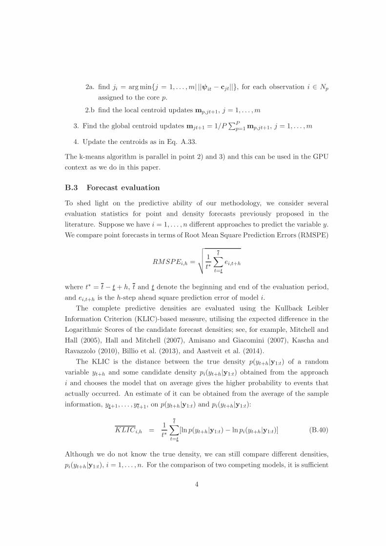
2a. find ji = argmin{j = 1, . . . ,m| ||ψit − cjt||}, for each observation i ∈ Np

assigned to the core p.

2.b find the local centroid updates mp,jt+1, j = 1, . . . ,m

3. Find the global centroid updates mjt+1 = 1/P∑P

p=1mp,jt+1, j = 1, . . . ,m

4. Update the centroids as in Eq. A.33.

The k-means algorithm is parallel in point 2) and 3) and this can be used in the GPU

context as we do in this paper.

B.3 Forecast evaluation

To shed light on the predictive ability of our methodology, we consider several

evaluation statistics for point and density forecasts previously proposed in the

literature. Suppose we have i = 1, . . . , n different approaches to predict the variable y.

We compare point forecasts in terms of Root Mean Square Prediction Errors (RMSPE)

RMSPEi,h =

√

√

√

√

1

t∗

t∑

t=t

ei,t+h

where t∗ = t − t + h, t and t denote the beginning and end of the evaluation period,

and ei,t+h is the h-step ahead square prediction error of model i.

The complete predictive densities are evaluated using the Kullback Leibler

Information Criterion (KLIC)-based measure, utilising the expected difference in the

Logarithmic Scores of the candidate forecast densities; see, for example, Mitchell and

Hall (2005), Hall and Mitchell (2007), Amisano and Giacomini (2007), Kascha and

Ravazzolo (2010), Billio et al. (2013), and Aastveit et al. (2014).

The KLIC is the distance between the true density p(yt+h|y1:t) of a random

variable yt+h and some candidate density pi(yt+h|y1:t) obtained from the approach

i and chooses the model that on average gives the higher probability to events that

actually occurred. An estimate of it can be obtained from the average of the sample

information, yt+1, . . . , yt+1, on p(yt+h|y1:t) and pi(yt+h|y1:t):

KLICi,h =1

t∗

t∑

t=t

[ln p(yt+h|y1:t)− ln pi(yt+h|y1:t)] (B.40)

Although we do not know the true density, we can still compare different densities,

pi(yt+h|y1:t), i = 1, . . . , n. For the comparison of two competing models, it is sufficient

4

to consider the Logarithmic Score (LS), which corresponds to the latter term in the

above sum,

LSi,h = −1

t∗

t∑

t=t

ln pi(yt+h|y1:t) (B.41)

for all i and to choose the model for which it is minimal, or, as we report in our tables

and use in the learning strategies, its opposite is maximal.

Secondly, we also evaluate density forecasts based on the continuous rank

probability score (CRPS); see, for example, Gneiting and Raftery (2007), Gneiting and

Ranjan (2013), Groen et al. (2013) and Ravazzolo and Vahey (2014). The CRPS for

the model i measures the average absolute distance between the empirical cumulative

distribution function (CDF) of yt+h, which is simply a step function in yt+h, and the

empirical CDF that is associated with model i’s predictive density:

CRPSi,t+h =

∫ +∞

−∞

(

F (z)− I[yt+h,+∞)(z))2

dz (B.42)

= Et|yi,t+h − yt+h| −1

2Et|y

∗i,t+h − y′i,t+h|

where F is the CDF from the predictive density pi(yt+h|y1:t) of model i and y∗i,t+h and

y′i,t+h are independent random variables with common sampling density equal to the

posterior predictive density pi(yt+h|y1:t). We report the sample average CRPS:

CRPSi,h = −1

t∗

t∑

t=t

CRPSi,t+h (B.43)

Smaller CRPS values imply higher precisions and, as for the log score, we report the

average CRPSi,h for each model i in all tables.

Finally, following Clark and Ravazzolo (2014), we apply the Diebold and Mariano

(1995) t-tests for equality of the average loss (with loss defined as squared error,

log score, or CRPS). In our tables presented below, differences in accuracy that

are statistically different from zero are denoted by one, two, or three asterisks,

corresponding to significance levels of 10%, 5%, and 1%, respectively. The underlying

p-values are based on t-statistics computed with a serial correlation-robust variance,

using the pre-whitened quadratic spectral estimator of Andrews and Monahan (1992).

Monte Carlo evidence in Clark and McCracken (2014) and Clark and McCracken

(2011) indicates that, with nested models, the Diebold-Mariano test compared against

5

50 100 150 200

−8

−6

−4

−2

0

2

4

6

8

Figure B.2: Gray area: the set of series (standardised for a better graphical representation),at the monthly frequency, of the Stock and Watson dataset. Solid line: growth rate of realGDP (seasonally adjusted) for the US. Dashed line: inflation measured as the change in theGDP deflator index (seasonally adjusted). Dotted line: yields on US government 90-day T-Bills (secondary market). Dashed-dotted: total employment growth rate for private industries(seasonally adjusted).

normal critical values can be viewed as a somewhat conservative (conservative in the

sense of tending to have size modestly below nominal size) test for equal accuracy in the

finite sample. Since the AR benchmark is always one of the model in the combination

schemes, we treat each combination as nesting the baseline, and we report p-values

based on one-sided tests, taking the AR as the null and the combination scheme in

question as the alternative.

B.4 Additional details and results on Stock and Watson (2005)

dataset

This section reports a detailed description of the cluster composition, in terms of

predictors, for the 5 and 7 clusters analysis of the series given in Fig. B.2, and

additional figures and tables related to their analysis and forecasting results.

The left and right columns in Fig. B.3) show the clusters of series in the parameter

space. The results show substantial evidence of different time series characteristics

in several groups of series. The groups are not well separated when looking at the

intercept values (see Fig. B.3, first and second row). However, the groups are well

6

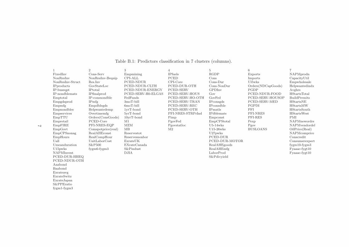
Table B.1: Predictors classification in 7 clusters (columns).

1 2 3 4 5 6 7FixedInv Cons-Serv Empmining IPfuels RGDP Exports NAPMprodnNonResInv NonResInv-Bequip CPI-ALL PCED Cons Imports CapacityUtilNonResInv-Struct Res.Inv PCED-NDUR CPI-Core Cons-Dur Ul5wks EmpwholesaleIPproducts GovStateLoc PCED-NDUR-CLTH PCED-DUR-OTH Cons-NonDur Orders(NDCapGoods) HelpwantedindxIP:buseqpt IPtotal PCED-NDUR-ENERGY PCED-SERV GPDInv PGDP AvghrsIP:nondblemats IPfinalprod PCED-SERV-H0-ELGAS PCED-SERV-HOUS Gov PCED-NDUR-FOOD HStartsTotalEmptotal IP:consnondble FedFunds PCED-SERV-HO-OTH GovFed PCED-SERV-HOUSOP BuildPermitsEmpgdsprod IPmfg 3moT-bill PCED-SERV-TRAN IPconsgds PCED-SERV-MED HStartsNEEmpmfg Empdblegds 6moT-bill PCED-SERV-REC IPconsdble PGPDI HStartsMWEmpnondbles Helpwantedemp 1yrT-bond PCED-SERV-OTH IPmatls PFI HStartsSouthEmpservices Overtimemfg 5yrT-bond PFI-NRES-STRPrInd IPdblemats PFI-NRES HStartsWestEmpTTU Orders(ConsGoods) 10yrT-bond Pimp Empconst PFI-RES PMIEmpretail PCED-Core M1 PgovFed EmpCPStotal Pexp NAPMnewordrsEmpFIRE PFI-NRES-EQP MZM Pgovstatloc U5-14wks Pgov NAPMvendordelEmpGovt Comspotprice(real) MB M2 U15-26wks BUSLOANS OilPrice(Real)EmpCPSnonag RealAHEconst Reservestot U27pwks NAPMcompriceEmpHours RealCompHour Reservesnonbor PCED-DUR ConscreditUall UnitLaborCost ExrateUK PCED-DUR-MOTOR ConsumerexpectUmeanduration S&P500 EXrateCanada RealAHEgoods fygm10-fygm3U15pwks fygm6-fygm3 S&Pindust RealAHEmfg Fyaaac-fygt10NAPMInvent DJIA LaborProd Fyaaac-fygt10PCED-DUR-HHEQ S&PdivyieldPCED-NDUR-OTHAaabondBaabondExrateavgExrateSwitzExrateJapanS&PPEratiofygm1-fygm3

7

−0.2 0 0.2 0.4 0.6−1

−0.5

0

0.5

11

23

4

5

α

β

−0.2 0 0.2 0.4 0.6−1

−0.5

0

0.5

1

12

34

5

6

7

αβ

−0.2 0 0.2 0.4 0.60

0.5

1

1.5

2

12

34

5

α

σ2

−0.2 0 0.2 0.4 0.60

0.5

1

1.5

2

1

2

3

4

56

7

α

σ2

−1 −0.5 0 0.5 10

0.5

1

1.5

2

12

34

5

β

σ2

−1 −0.5 0 0.5 10

0.5

1

1.5

2

1

2

3

4

56

7

β

σ2

Figure B.3: Pairwise scatter plots of the series features: αi and βi (first row), αi and σ2

i

(second row) and βi and σ2

i (last row). In each plot the red dots represent the cluster means.We assume alternatively 5 (left) and 7 (right) clusters.

8

separated along two directions of the parameter space, which are the one associated

with the variance and the one associated with persistence parameters (Fig. B.3, last

row). The differences in terms of persistence, in the different groups, is also evident

from the heat maps given in Fig. B.4. Different gray levels in the two graphs show

the value of the variables (horizontal axis) over time (vertical axis). The vertical red

lines indicate the different clusters. One can see for example that the series in the

2nd and 4th cluster (of 5) are more persistent then the series in the clusters 1, 3 and

5 (see also Fig. B.3, bottom left). Series in cluster 1, 2 and 4 are less volatile than

series in the cluster 3 and 5. This information is also summarised by the mean value of

the parameter estimates for the series that belong to the same cluster. See the values

in Table B.4. Looking at the composition of the predictor groups (see also Tables

B.2-B.3), we find that:

1. The first cluster comprises capacity utilisation, employment variables, housing

(building permits and new ownership started) and manufacturing variables (new

orders, supplier deliveries index, inventories).

2. The second cluster contains exports, a large numbers of price indexes (e.g. prices

indexes for personal consumption expenditures, and for gross domestic product)

some money market variables (e.g. M1 and M2).

3. The third cluster includes real gross domestic product, consumption and

consumption of non-durables, some industrial production indexes, and some

financial market variables (e.g., S&P industrial, corporate bonds and USD -

GBP exchange rate).

4. The fourth cluster includes imports, some price indexes and financials such as

government debt (3- and 6-months T-bills and 5- and 10-years T-bonds), stocks

and exchange rates.

5. The fifth cluster mainly includes investments, industrial production indexes

(total and many sector indexes), and employment.

9

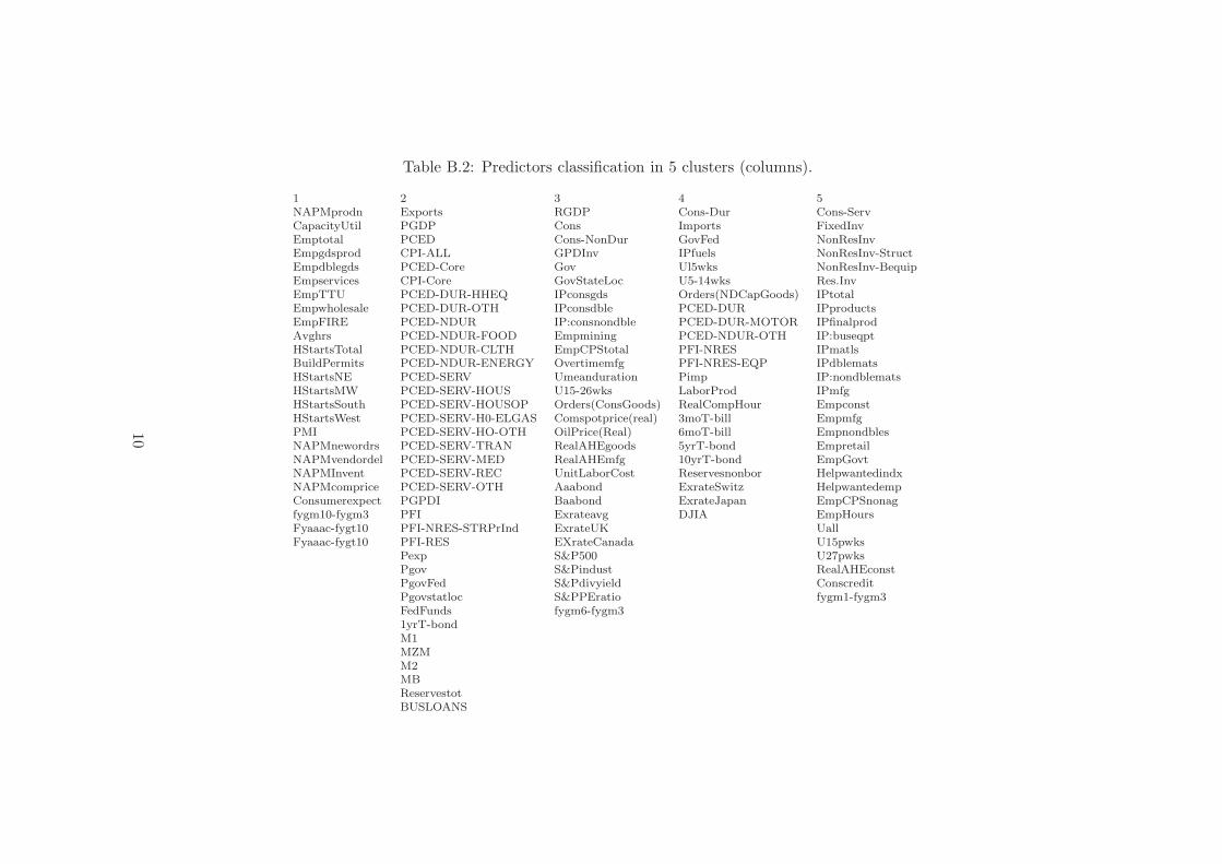
Table B.2: Predictors classification in 5 clusters (columns).

1 2 3 4 5NAPMprodn Exports RGDP Cons-Dur Cons-ServCapacityUtil PGDP Cons Imports FixedInvEmptotal PCED Cons-NonDur GovFed NonResInvEmpgdsprod CPI-ALL GPDInv IPfuels NonResInv-StructEmpdblegds PCED-Core Gov Ul5wks NonResInv-BequipEmpservices CPI-Core GovStateLoc U5-14wks Res.InvEmpTTU PCED-DUR-HHEQ IPconsgds Orders(NDCapGoods) IPtotalEmpwholesale PCED-DUR-OTH IPconsdble PCED-DUR IPproductsEmpFIRE PCED-NDUR IP:consnondble PCED-DUR-MOTOR IPfinalprodAvghrs PCED-NDUR-FOOD Empmining PCED-NDUR-OTH IP:buseqptHStartsTotal PCED-NDUR-CLTH EmpCPStotal PFI-NRES IPmatlsBuildPermits PCED-NDUR-ENERGY Overtimemfg PFI-NRES-EQP IPdblematsHStartsNE PCED-SERV Umeanduration Pimp IP:nondblematsHStartsMW PCED-SERV-HOUS U15-26wks LaborProd IPmfgHStartsSouth PCED-SERV-HOUSOP Orders(ConsGoods) RealCompHour EmpconstHStartsWest PCED-SERV-H0-ELGAS Comspotprice(real) 3moT-bill EmpmfgPMI PCED-SERV-HO-OTH OilPrice(Real) 6moT-bill EmpnondblesNAPMnewordrs PCED-SERV-TRAN RealAHEgoods 5yrT-bond EmpretailNAPMvendordel PCED-SERV-MED RealAHEmfg 10yrT-bond EmpGovtNAPMInvent PCED-SERV-REC UnitLaborCost Reservesnonbor HelpwantedindxNAPMcomprice PCED-SERV-OTH Aaabond ExrateSwitz HelpwantedempConsumerexpect PGPDI Baabond ExrateJapan EmpCPSnonagfygm10-fygm3 PFI Exrateavg DJIA EmpHoursFyaaac-fygt10 PFI-NRES-STRPrInd ExrateUK UallFyaaac-fygt10 PFI-RES EXrateCanada U15pwks

Pexp S&P500 U27pwksPgov S&Pindust RealAHEconstPgovFed S&Pdivyield ConscreditPgovstatloc S&PPEratio fygm1-fygm3FedFunds fygm6-fygm31yrT-bondM1MZMM2MBReservestotBUSLOANS

10

Table B.3: Predictors classification in 7 clusters (columns).

1 2 3 4 5 6 7FixedInv Cons-Serv Empmining IPfuels RGDP Exports NAPMprodnNonResInv NonResInv-Bequip CPI-ALL PCED Cons Imports CapacityUtilNonResInv-Struct Res.Inv PCED-NDUR CPI-Core Cons-Dur Ul5wks EmpwholesaleIPproducts GovStateLoc PCED-NDUR-CLTH PCED-DUR-OTH Cons-NonDur Orders(NDCapGoods) HelpwantedindxIP:buseqpt IPtotal PCED-NDUR-ENERGY PCED-SERV GPDInv PGDP AvghrsIP:nondblemats IPfinalprod PCED-SERV-H0-ELGAS PCED-SERV-HOUS Gov PCED-NDUR-FOOD HStartsTotalEmptotal IP:consnondble FedFunds PCED-SERV-HO-OTH GovFed PCED-SERV-HOUSOP BuildPermitsEmpgdsprod IPmfg 3moT-bill PCED-SERV-TRAN IPconsgds PCED-SERV-MED HStartsNEEmpmfg Empdblegds 6moT-bill PCED-SERV-REC IPconsdble PGPDI HStartsMWEmpnondbles Helpwantedemp 1yrT-bond PCED-SERV-OTH IPmatls PFI HStartsSouthEmpservices Overtimemfg 5yrT-bond PFI-NRES-STRPrInd IPdblemats PFI-NRES HStartsWestEmpTTU Orders(ConsGoods) 10yrT-bond Pimp Empconst PFI-RES PMIEmpretail PCED-Core M1 PgovFed EmpCPStotal Pexp NAPMnewordrsEmpFIRE PFI-NRES-EQP MZM Pgovstatloc U5-14wks Pgov NAPMvendordelEmpGovt Comspotprice(real) MB M2 U15-26wks BUSLOANS OilPrice(Real)EmpCPSnonag RealAHEconst Reservestot U27pwks NAPMcompriceEmpHours RealCompHour Reservesnonbor PCED-DUR ConscreditUall UnitLaborCost ExrateUK PCED-DUR-MOTOR ConsumerexpectUmeanduration S&P500 EXrateCanada RealAHEgoods fygm10-fygm3U15pwks fygm6-fygm3 S&Pindust RealAHEmfg Fyaaac-fygt10NAPMInvent DJIA LaborProd Fyaaac-fygt10PCED-DUR-HHEQ S&PdivyieldPCED-NDUR-OTHAaabondBaabondExrateavgExrateSwitzExrateJapanS&PPEratiofygm1-fygm3

11

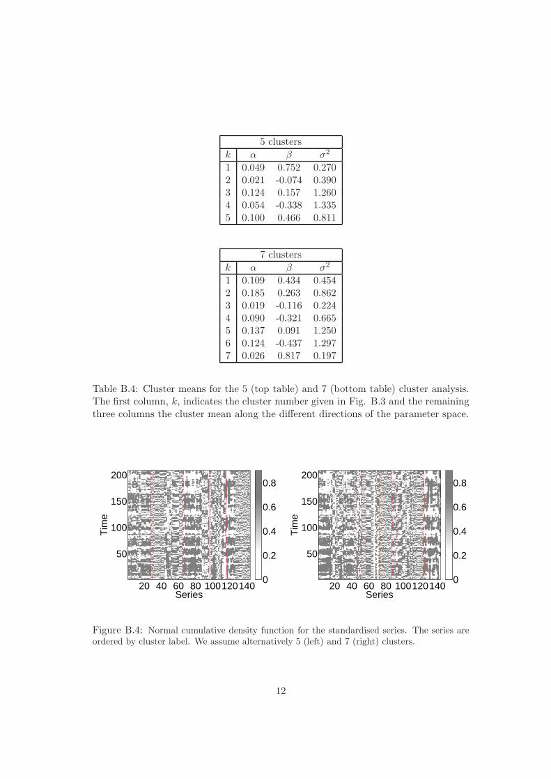
5 clusters

k α β σ2

1 0.049 0.752 0.2702 0.021 -0.074 0.3903 0.124 0.157 1.2604 0.054 -0.338 1.3355 0.100 0.466 0.811

7 clusters

k α β σ2

1 0.109 0.434 0.4542 0.185 0.263 0.8623 0.019 -0.116 0.2244 0.090 -0.321 0.6655 0.137 0.091 1.2506 0.124 -0.437 1.2977 0.026 0.817 0.197

Table B.4: Cluster means for the 5 (top table) and 7 (bottom table) cluster analysis.The first column, k, indicates the cluster number given in Fig. B.3 and the remainingthree columns the cluster mean along the different directions of the parameter space.

Series

Tim

e

20 40 60 80 100120140

50

100

150

200

0

0.2

0.4

0.6

0.8

Series

Tim

e

20 40 60 80 100120140

50

100

150

200

0

0.2

0.4

0.6

0.8

Figure B.4: Normal cumulative density function for the standardised series. The series areordered by cluster label. We assume alternatively 5 (left) and 7 (right) clusters.

12

1985Q1 1995Q1 2005Q1 2011Q20

0.1

0.2

0.3

0.4

0.5

0.6

0.7

w11t

w12t

w13t

w14t

w15t

w16t

w17t

1985Q1 1995Q1 2005Q1 2011Q20

0.1

0.2

0.3

0.4

0.5

w11t

w12t

w13t

w14t

w15t

w16t

w17t

1985Q1 1995Q1 2005Q1 2011Q20

0.1

0.2

0.3

0.4

0.5

w11t

w12t

w13t

w14t

w15t

w16t

w17t

1985Q1 1995Q1 2005Q1 2011Q20

0.1

0.2

0.3

0.4

0.5

w21t

w22t

w23t

w24t

w25t

w26t

w27t

1985Q1 1995Q1 2005Q1 2011Q20

0.1

0.2

0.3

0.4

w21t

w22t

w23t

w24t

w25t

w26t

w27t

1985Q1 1995Q1 2005Q1 2011Q20

0.1

0.2

0.3

0.4

0.5

w21t

w22t

w23t

w24t

w25t

w26t

w27t

1985Q1 1995Q1 2005Q1 2011Q20

0.1

0.2

0.3

0.4

0.5

w31t

w32t

w33t

w34t

w35t

w36t

w37t

1985Q1 1995Q1 2005Q1 2011Q20

0.1

0.2

0.3

0.4

0.5

w31t

w32t

w33t

w34t

w35t

w36t

w37t

1985Q1 1995Q1 2005Q1 2011Q20

0.1

0.2

0.3

0.4

0.5

w31t

w32t

w33t

w34t

w35t

w36t

w37t

1985Q1 1995Q1 2005Q1 2011Q20

0.1

0.2

0.3

0.4

0.5

w41t

w42t

w43t

w44t

w45t

w46t

w47t

1985Q1 1995Q1 2005Q1 2011Q20

0.1

0.2

0.3

0.4

0.5

w41t

w42t

w43t

w44t

w45t

w46t

w47t

1985Q1 1995Q1 2005Q1 2011Q20

0.1

0.2

0.3

0.4

0.5

0.6

0.7

w41t

w42t

w43t

w44t

w45t

w46t

w47t

Figure B.5: In each plot the mean logistic-normal weights (different lines) for the univariatecombination model are given. Rows: plot for the four series of interest (real GDP growth rate,GDP deflator, 3-month Treasury Bills, employment). Columns: forecast horizons (1, 3 and 5quarters).

13

1985Q1 1995Q1 2005Q1 2011Q20

0.2

0.4

0.6

0.8

1

1985Q1 1995Q1 2005Q1 2011Q20

0.2

0.4

0.6

0.8

1

1985Q1 1995Q1 2005Q1 2011Q20

0.1

0.2

0.3

0.4

0.5

1985Q1 1995Q1 2005Q1 2011Q20

0.2

0.4

0.6

0.8

1

1985Q1 1995Q1 2005Q1 2011Q20

0.2

0.4

0.6

0.8

1

1985Q1 1995Q1 2005Q1 2011Q20

0.2

0.4

0.6

0.8

1

1985Q1 1995Q1 2005Q1 2011Q20

0.1

0.2

0.3

0.4

0.5

Figure B.6: The plots show the model weights (bk,ij) in each cluster (i = j) when forecastingGDP growth (k = 1) at the 1-step ahead horizon. The first row refers to clusters 1, 2, and 3;the second row to clusters 4, 5, and 6; the last row to cluster 7.

14

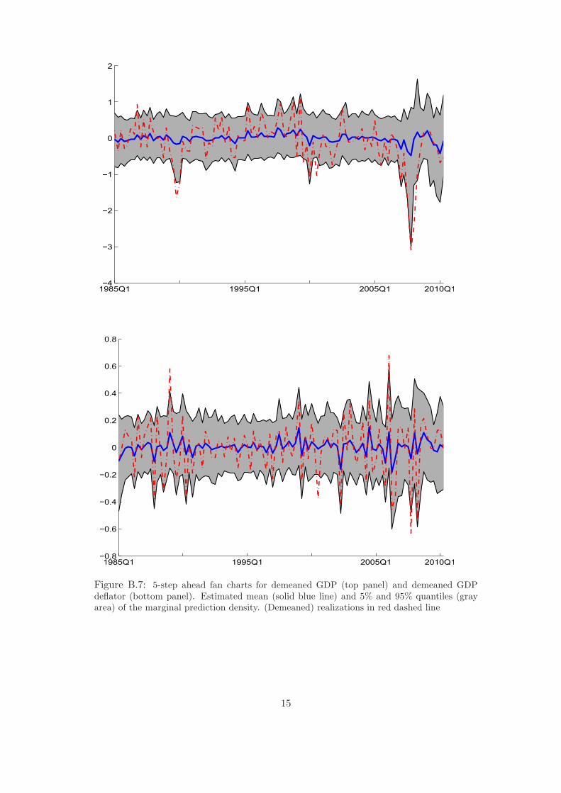
1985Q1 1995Q1 2005Q1 2010Q14

3

2

1

0

1

2

1985Q1 1995Q1 2005Q1 2010Q1−0.8

−0.6

−0.4

−0.2

0

0.2

0.4

0.6

0.8

Figure B.7: 5-step ahead fan charts for demeaned GDP (top panel) and demeaned GDPdeflator (bottom panel). Estimated mean (solid blue line) and 5% and 95% quantiles (grayarea) of the marginal prediction density. (Demeaned) realizations in red dashed line

15

B.5 Computing time

In this section we compare the computational speed of CPU with GPU in the

implementation of our combination algorithm for both the financial and macro

application. Whether CPU computing is standard in econometrics, GPU approach

to computing has been received large attention in economics only recently. See, for

example, Aldrich (2013) for a review, Geweke and Durham, 2012 and Lee et al., 2010

for applications to Bayesian inference and Aldrich et al., 2011, Morozov and Mathur,

2012 and Dziubinski and Grassi, 2013 for solving DSGE models.

The CPU and the GPU versions of the computer program are written in MATLAB,

as described in Casarin et al. (2015). In the CPU setting, our test machine is a server

with two Intel Xeon CPU E5-2667 v2 processors and a total of 32 core. In the first

GPU setting, our test machine is a NVIDIA Tesla K40c GPU. The Tesla K40c card

is with 12GB memory and 2880 cores and it is installed in one of the cores of the

CPU server. In the second GPU setting, our test machine is a NVIDIA GeForce GTX

660 GPU card, which is a middle-level video card, with a total of 960 cores. The test

machine is a desktop Windows 8 machine, has 16 GB of Ram and only requires a

MATLAB parallel toolbox license.

We compare two sets of combination experiments, the density combination based

on 4 clusters with equal weights within clusters and time-varying volatility, DCEW-

SV, see Section 5, and the density combination with univariate combination based on

7 clusters with recursive log score weights within clusters, UDCLS75, see Section 5.2,

for an increasing number of particles N . In both sets of experiments we calculated, in

seconds, the overall average execution time reported in Table B.5.

As the table shows, the CPU implementation is slower then the first GPU set-up in

all cases. The NVIDIA Tesla K40c GPU provides gains in the order of magnitude from

2 to 4 times than the CPU. Very interestingly, even the second GPU set-up, which can

be installed in a desktop machine, provides execution times comparable to the CPU

in the financial applications and large gains in the macro applications. Therefore, the

GPU environment seems the preferred one for our density combination problems and

when the number of predictive density becomes very large a GPU server card gives

the highest gains.

5The case MCDCLS7 provide similar relative timing, in absolute terms a bit faster than theunivariate ones.

16

DCEW-SV UDCLS7Draws 100 500 1000 100 500 1000

CPU 1032 5047 10192 5124 25683 51108GPU 1 521 2107 4397 1613 6307 14017GPU 2 1077 5577 13541 2789 13895 27691

Ratio 1 1.98 2.39 2.32 3.18 4.07 3.65Ratio 2 0.96 0.90 0.75 1.84 1.85 1.85

Table B.5: Observed total time (in seconds) and CPU/GPU ratios for the algorithm on CPUand GPU on different machines and with different numbers of particles. The CPU is a 32core Intel Xeon CPU E5-2667 v2 two processors and the GPU1 is a NVIDIA Tesla K40c GPUand the GPU2 is a NVIDIA GeForce GTX 660. “Ratio 1” refers to the CPU/GPU 1 ratioand “ratio 2” refers to the CPU/GPU 2 ratios. Number below 1 indicates the CPU is faster,number above one indicates that the GPU is faster.

17

References

Aastveit, K., Gerdrup, K., Jore, A., and Thorsrud, L. (2014). Nowcasting GDP in real-

time: A density combination approach. Journal of Business Economics & Statistics,

32:48–68.

Aldrich, E. M. (2013). Massively Parallel Computing in Economics. Technical report,

University of California, Santa Cruz.

Aldrich, E. M., Fernandez-Villaverde, J., Gallant, A. R., and Rubio Ramırez,

J. F. (2011). Tapping the Supercomputer Under Your Desk: Solving Dynamic

Equilibrium Models with Graphics Processors. Journal of Economic Dynamics and

Control, 35:386–393.

Amisano, G. and Giacomini, R. (2007). Comparing density forecasts via weighted

likelihood ratio tests. Journal of Business & Economic Statistics, 25:177–190.

Andrews, D. and Monahan, J. (1992). An improved heteroskedasticity and

autocorrelation consistent covariance matrix estimator. Econometrica, 60:953–966.

Billio, M., Casarin, R., Ravazzolo, F., and van Dijk, H. K. (2013). Time-

varying Combinations of Predictive Densities Using Nonlinear Filtering. Journal

of Econometrics, 177:213–232.

Casarin, R., Grassi, S., Ravazzolo, F., and van Dijk, H. (2015). Parallel sequential

Monte Carlo for efficient density combination: the DeCo Matlab toolbox. Jounal of

Statistical Software, forthcoming.

Clark, T. and McCracken, M. W. (2011). Testing for unconditional predictive ability.

In Clements, M. and Hendry, D., editors, Oxford Handbook of Economic Forecasting.

Oxford University Press, Oxford.

Clark, T. and McCracken, M. W. (2014). Nested forecast model comparisons: a new

approach to testing equal accuracy. Journal of Econometrics, forthcoming.

Clark, T. and Ravazzolo, F. (2014). The macroeconomic forecasting performance

of autoregressive models with alternative specifications of time-varying volatility.

Journal of Applied Econometrics, forthcoming.

Diebold, F. X. and Mariano, R. S. (1995). Comparing predictive accuracy. Journal of

Business and Economic Stastistics, 13:253–263.

18

Dziubinski, M. P. and Grassi, S. (2013). Heterogeneous computing in economics: A

simplified approach. Computational Economics, 43:485–495.

Geweke, J. and Durham, G. (2012). Massively parallel sequential Monte Carlo for

Bayesian inference. Working papers, National Bureau of Economic Research, Inc.

Gneiting, T. and Raftery, A. E. (2007). Strictly proper scoring rules, prediction, and

estimation. Journal of the American Statistical Association, 102:359–378.

Gneiting, T. and Ranjan, R. (2013). Combining predicitve distributions. Electronic

Journal of Statistics, 7:1747–1782.

Groen, J., Paap, R., and Ravazzolo, F. (2013). Real-time inflation forecasting in a

changing world. Journal of Business & Economic Stastistics, 31:29–44.

Hall, S. G. and Mitchell, J. (2007). Combining density forecasts. International Journal

of Forecasting, 23:1–13.

Kascha, C. and Ravazzolo, F. (2010). Combining inflation density forecasts. Journal

of Forecasting, 29:231–250.

Lee, A., Yau, C., Giles, M., Doucet, A., and Holmes, C. (2010). On the utility of

graphic cards to perform massively parallel simulation with advanced Monte Carlo

methods. Journal of Computational and Graphical Statistics, 19:769 – 789.

Marcellino, M., Stock, J., and Watson, M. (2006). A comparison of direct and

iterated multistep ar methods for forecasting macroeconomic time series. Journal

of Econometrics, (135):499–526.

Mitchell, J. and Hall, S. G. (2005). Evaluating, comparing and combining density

forecasts using the KLIC with an application to the Bank of England and NIESER

“fan” charts of inflation. Oxford Bulletin of Economics and Statistics, 67:995–1033.

Morozov, S. and Mathur, S. (2012). Massively parallel computation using graphics

processors with application to optimal experimentation in dynamic control.

Computational Economics, 40:151–182.

Ravazzolo, F. and Vahey, S. V. (2014). Forecast densities for economic aggregates

from disaggregate ensembles. Studies in Nonlinear Dynamics and Econometrics,

18:367–381.

Stock, J. H. and Watson, W. M. (2005). Implications of dynamic factor models for

VAR analysis. Technical report, NBER Working Paper No. 11467.

19