Dynamical chaos: systems of classical mechanicschaos.phys.msu.ru/loskutov/PDF/UFN_1_Eng.pdf ·...

Abstract. This article is a methodological manual for those whoare interested in chaotic dynamics. An exposition is given on thefoundations of the theory of deterministic chaos that originatesin classical mechanics systems. Fundamental results obtained inthis area are presented, such as elements of the theory of non-linear resonance and the Kolmogorov ±Arnol'd ±Moser theory,the PoincareÂ ± Birkhoff fixed-point theorem, and theMel'nikovmethod. Particular attention is given to the analysis of thephenomena underlying the self-similarity and nature of chaos:splitting of separatrices and homoclinic and heteroclinic tan-gles. Important properties of chaotic systems Ð unpredictabil-ity, irreversibility, and decay of temporal correlations Ð aredescribed. Models of classical statistical mechanics with chao-tic properties, which have become popular in recent years Ðbilliards with oscillating boundaries Ð are considered. It isshown that if a billiard has the property of well-developedchaos, then perturbations of its boundaries result in Fermiacceleration. But in nearly-integrable billiard systems, excita-

tions of the boundaries lead to a new phenomenon in the en-semble of particles, separation of particles in accordance theirvelocities. If the initial velocity of the particles exceeds a certaincritical value characteristic of the given billiard geometry, theparticles accelerate; otherwise, they decelerate.

1. Introduction

For a long time, the concept of chaos was associated with theassumption that, at least, the excitation of an extremely highnumber of degrees of freedom is necessary in the system. Theformation of this idea seems to have been influenced by theconcepts of statistical mechanics, in which the motion of anindividual gas particle can be predicted in principle but thebehavior of a system consisting of a huge number of particlesis extremely complex, and therefore a detailed dynamicapproach is meaningless. This dictated the need for astatistical analysis. But extensive studies have demonstratedthat the validity of the statistical laws and statisticaldescription is not restricted to highly complex systems witha large number of the degrees of freedom. Random behaviorcan also be exhibited by entirely deterministic systems with amoderate number of the degrees of freedom.Here, the point isnot the complexity of the system or the presence of externalnoise but the emergence of an exponential instability ofmotion at certain values of the parameters. The dynamics ofsystems subject to such an instability is called dynamicstochasticity, or deterministic (dynamic) chaos. Investiga-

A Loskutov Physics Department, Lomonosov Moscow State University,

Vorob'evy gory, 119992 Moscow, Russian Federation

Tel. (7-495) 939 51 56. Fax (7-495) 939 29 88

E-mail: [email protected]

Received 31 January 2007, revised 25 April 2007

Uspekhi Fizicheskikh Nauk 177 (9) 989 ± 1015 (2007)

Translated by A V Getling; edited by AM Semikhatov

METHODOLOGICAL NOTES PACS numbers: 05.45. ë a, 05.45.Ac

Dynamical chaos: systems of classical mechanics

A Loskutov

DOI: 10.1070/PU2007v050n09ABEH006341

Contents

1. Introduction 9392. Background 9413. Hamiltonian mechanics 942

3.1 Integrable systems; 3.2 Perturbed motion

4. Nonlinear resonance 9434.1 Small denominators; 4.2 Universal Hamiltonian; 4.3 Width of the separatrix; 4.4 Internal resonances;

4.5 Overlapping of resonances; 4.6 Higher-order resonances

5. Elements of the Kolmogorov ±Arnol'd ±Moser theory 9475.1 The Kolmogorov theorem; 5.2 The Arnol'd diffusion

6. The nature of chaos 9496.1 Twist map; 6.2 Fixed-point theorem; 6.3 Elliptic and hyperbolic points; 6.4 Splitting of separatrices. Homoclinic

tangles

7. The Mel'nikov method 9527.1 The Mel'nikov function; 7.2 The Duffing oscillator and nonlinear pendulum

8. Principal properties of chaotic systems 9548.1 Ergodicity and mixing; 8.2 Unpredictability and irreversibility; 8.3 Decay of correlations

9. Billiards 9569.1 The Lorentz gas; 9.2 Scattering billiards with oscillating boundaries. The Fermi acceleration; 9.3 Focusing billiards

with oscillating boundaries. Particle deceleration

10. Conclusion 960References 961

Physics ±Uspekhi 50 (9) 939 ± 964 (2007) # 2007 Uspekhi Fizicheskikh Nauk, Russian Academy of Sciences

tions in this area are of fundamental importance because theydisclose the nature of randomness by supplementing thehypothesis of molecular chaos with the hypothesis ofdynamic stochasticity.

H PoincareÂ [1] was the first to note the relation betweenstatistics and instabilities. However, a statistical approach tothe description of systems with numerous degrees of freedomwas previously suggested by L Boltzmann [2], who conjec-tured that the motion of particles in a rarefied gas should beregarded as random and that the entire energetically allowedphase-space domain is accessible to each particle. Such a viewof the properties of multiparticle systems, known as theergodic hypothesis [2 ± 4], became the basis of classicalstatistical mechanics. A rigorous substantiation of thishypothesis could not be found for a long time, however.Some progress in this direction was achieved due to studies byP Ehrenfest [5, 6] (see also Refs [7, 8]). In particular, theyallowed establishing applicability limits for the laws ofstatistical mechanics. However, a well-known study byE Fermi, J Pasta, and S Ulam [9] (see Refs [10, 11] for amore detailed exposition), who made the first attempt toverify the ergodicity hypothesis, put the problem of sub-stantiation of statistical physics in the forefront again.

This problem can be partially resolved based on studies byPoincareÂ (see Ref. [12]), who concluded that the motion of asystem is extremely complex in the neighborhood of unstablefixed points in phase space. This was the earliest indication ofthe possible chaotic properties of nonlinear dynamicalsystems. Later, G D Birkhoff [13] showed that if the ratio ofthe frequencies is rational (i.e., at a resonance), stable andunstable fixed points appear in phase space. Higher-orderresonances change the topology of phase trajectories and leadto the formation of a chain of `islands.' It turned out that theregular perturbation theory fails to describe such resonances,because the solutions are strongly perturbed near theresonances, and therefore small denominators emerge in theexpansion and the series diverge.

N S Krylov [14] was the first to deeply investigate thenature of statistical laws. He showed that the property ofmixing and the related local instability of nearly all trajec-tories of the corresponding dynamical systems underlie thisnature. In view of this, M Born [15] (see also [16]) suggestedthat the behavior of the systems is not predictable in classicalmechanics. Later, the dynamics due to such instabilities in thesystems came to be known as dynamic stochasticity, ordeterministic (dynamic) chaos. The word `chaos,' in thismeaning, seems to have been introduced by J A Yorke [17](see Ref. [18], p. 338). But as noted by Ya G Sinai, the wordcombination `deterministic chaos' was first used by B Chir-ikov and G Ford in the 1960s.

Physically, due to unavoidable fluctuations (i.e., smallperturbations of the initial conditions), the initial state of thesystem is to be specified by some distribution. The problem isin predicting the evolution of the system based on this initialdistribution. If the system is stable, such that small perturba-tions do not increase exponentially with time, its behavior ispredictable. In contrast, if the system is subject to exponentialinstability (which is expressed by saying that the system has asensitive dependence on the initial conditions), the processallows only a probabilistic description. In essence, preciselythese considerations formed the basis of the modern views ofdynamical chaos. The discovery that it is chaos, rather thanexternal noise, that mainly determines the behavior of thesystem was unexpected (see Ref. [20] for a review).

The schools of A N Kolmogorov and A A Andronov, towhich a brilliant group of outstanding contemporary math-ematicians belongs, have deeply influenced the developmentof the theory of dynamical chaos. In particular, Kolmogor-ov's theorem of the preservation of almost periodic motionin weakly perturbed Hamiltonian systems, proved byV I Arnol'd and J Moser and known as the Kolmogorov ±Arnol'd ±Moser (KAM) theorem (see Refs [21 ± 25]),became a keystone in understanding the origin of chaoticbehavior. In their early studies, D V Anosov [26] and Sinai[27, 28] showed that dynamical chaos is a widespreadphenomenon.

In his pioneering investigations of the bifurcations of asaddle ± focus separatrix [29, 30], L P Shil'nikov developed,among other things, a special technique for the analysis of thedynamics of systems near saddle-type trajectories anduncovered the extreme complexity of the structures thatdevelop as homoclinic trajectories appear. It was demon-strated that the behavior of systems must be complex in thefull neighborhood of the parametric values at which ahomoclinic orbit exists. Later, Shil'nikov, L M Lerman,N K Gavrilov, I M Ovsyannikov, D V Turaev, and othersdeveloped new methods that allowed describing a finitenumber of bifurcations that lead to chaotic dynamics (seeRefs [31, 32] and the references therein).

A new stage in explaining chaotic behavior and its originin deterministic systems was initiated by Kolmogorov's andSinai's studies [33 ± 35], where the concept of entropy wasintroduced for dynamical systems. These studies laid thefoundations of a consistent theory of chaotic dynamicalsystems.

Various abstract mathematical constructions have playedan important role in the development of the theory ofdeterministic chaos. In particular, S Smale [36], to disprovethe hypothesis of the density of systems that exhibit only aperiodic-type behavior, constructed a notable example,currently known as the `Smale horseshoe.' This exampleimplies that there exist systems that have both an infinitenumber of periodic orbits with different periods and aninfinite number of aperiodic trajectories [18, 36, 37]. Sub-sequent to the Smale horseshoe, Anosov's C-systems werefound [26, 38], which are characterized by the most pro-nounced mixing properties. Such systems were generalized byintroducing Smale's `Axiom A' [37] (see also Refs [39 ± 41]and the references therein) and hyperbolic sets [18, 37, 40 ±42]; these generalizations specified an important class ofdynamical systems that have the property of the exponentialinstability of trajectories (see Ref. [43] for a review).

At nearly the same time, mathematical studies beganappearing in which attempts were made to substantiatestatistical mechanics based on the analysis of billiardsystems [27, 28]. Originally, billiards were introduced assimplified models appropriate for the consideration ofcertain problems of statistical physics [13] (see also thereferences in Refs [44, 45]). A billiard on a plane is adynamical system that describes bodies (balls) movinginertially inside a bounded domain, in accordance with thelaw of equality of the incidence and reflection angles. Inessence, planar mathematical billiards are the usual billiardswithout friction, although with an arbitrary configuration ofthe table and without pockets.

Krylov's problem ofmixing in a system of elastic balls [14]was first solved using billiard systems. Furthermore, it wasshown that systems corresponding to billiards with scattering

940 A Loskutov Physics ±Uspekhi 50 (9)

boundaries have much in common with geodesic flows innegative-curvature spaces, i.e., withAnosov flows. Somewhatlater, the class of billiard systems capable of exhibitingchaotic properties was substantially extended (see Refs [45 ±47] and the references therein). It was shown based on ageneralization of such systems (a modified two-dimensionalLorentz gas) that motion in purely deterministic systems canbe similar to Brownianmotion [44, 45]. This result became thefirst rigorous confirmation of chaotic properties exhibited bydynamical systems (not involving any random mechanism).

Further investigations of nonlinear systems, both theore-tical and experimental, have shown how typical the chaoticbehavior is in systems with few degrees of freedom. It becameobvious that chaotic properties can bemanifested by a varietyof nonlinear systems; if chaos is not revealed, this can merelyresult from the fact that the development of chaos is restrictedeither to very small domains in the parameter space or tophysically unrealizable domains.

How does chaotic motion originate? What is the nature ofchaos? Seemingly, there should be many paths toward theonset of chaos. But it became known that the scenarios ofchaotization are far from numerous.Moreover, some of themobey universal laws and are independent of the nature of thesystem. The same development scenarios for chaos areinherent in a variety of objects. The universal behaviorresembles the usual second-order phase transitions, andinvoking renormalization-group and scaling techniquesknown in statistical mechanics opens new avenues ininvestigating chaotic dynamics.

This article presents the foundations of the theory ofdynamical chaos. We describe the principal results obtainedin the field that belong to classical mechanics, such aselements of the theory of nonlinear resonance and theKAM theory; the PoincareÂ ± Birkhoff fixed-point theorem,which is important for understanding the sources of chaoticbehavior; and the Mel'nikov method, which allowed obtain-ing a criterion for the origin of chaos analytically in somecases. Particular attention is given to the nature of chaos.Specifically, we detail the factors that lead perturbed systemsto manifest self-similarity, to the splitting of separatrices,and to homoclinic and heteroclinic tangles. We also showthat unpredictability, irreversibility, and decay of temporalcorrelations occur in systems in which such phenomena areobserved.

In Section 9, we describe models of nonequilibriumclassical statistical mechanics with chaotic properties, highlypopular today: billiards with oscillating boundaries. TheLorentz gas and stadium-type billiards are considered indetail. An interesting result is presented: the analytic form ofbilliard-particle acceleration law, i.e., a proof of the presenceof Fermi acceleration in billiards with well-developed chaos.But if a billiard system is near an integrable system, such thatthe curvature of the billiard boundary is not large, smalloscillations of the boundary lead to a new phenomenon. Aspecific, billiard version of Maxwell's demon originates: abilliard particle either accelerates or decelerates depending onthe initial conditions. In other words, perturbation of theboundaries of such billiards results in a velocity stratificationof the particle ensemble.

The modern mathematical techniques used to analyze thechaotic properties of dynamical systems are fairly complex.But in this article, we pursue the aim of giving a general idea ofthe origin of the phenomenon of deterministic chaos andexpose the fundamental concepts underlying the currently

known approaches to chaotic dynamics. Therefore, ourpresentation is mainly based on geometric techniques and aqualitative approach. Although most of the results describedhere have been known for a rather long time, we present themin a form appropriate for a nonexpert to comprehend theorigins of chaotic dynamics. Therefore, in particular, thisarticle is methodological.

2. Background

The subject of our analysis is the systems described byordinary differential equations

_x � v�x; a� ; �1�

where v � fv1; v2; . . . ; vlg is a vector function (typicallyassumed to be smooth), a symbolizes the set of parameters,and x � fx1; x2; . . . ; xlg is an l-dimensional vector withcomponents x1; x2; . . . ; xl that characterizes the state of adynamical system. If the substitution of a function F�t; ci�,ci � const, in Eqn (1) turns them into identities, this functionis called a solution. Specifying initial conditions x�0� � x0uniquely determines the solution at any instant t,

x�t� � F�t; x0� : �2�

Any solution x�t� of system of equations (1) can begeometrically represented by a curve in the l-dimensionalspace of variables x1; . . . ; xl. This l-dimensional space is calledthe phase space of the system (we let M denote this space).Each state of the dynamical system corresponds to a point inM, and each point in M corresponds to a unique state of thesystem. Changes in the state of the system can be interpretedas the motion of a point (called the representation point) inthe phase space. The trajectory of this representation point,i.e., the set of its consecutive positions in the phase spaceM, iscalled the phase trajectory.

We assume that system (1), whose phase space isM, was inthe state x0 at an instant t0. Then, generally, it is in anotherstate at an instant t 6� t0. We let F tx0 denote this new state.Thus, for any t, we define the evolution operator, or the shiftmap F t : M!M of the phase spaceM into itself. ThemapF t

transforms the system from its state at t0 into the state at t. Inother words, solution (2) of Eqns (1) establishes a correspon-dence between the point xi�t0�, i � 1; 2; . . . ; l, of the phasespaceM at the instant t0 and a certain phase-space point xi�t�at an instant t:

F tx0 � x�t� : �3�

Therefore, in the general case, any phase-space domain O0

transforms in time t into another domain, Ot � F tO0, underthe action of the map F t. The map F t : M!M is also calledthe phase flow, and the function v�x� is the vector field of thegiven dynamical system whose phase space isM.

If the phase flow F t has a secant S, i.e., a certaincodimension-1 hypersurface that is transversally intersectedby phase curves, then a mapF can be defined on S as follows:to any point p of S we associate the closest (next to p) point,p 0, of intersection of the phase curve with the same hypersur-face S. Then the analysis of the dynamics of the originalsystem reduces to analyzing the properties of the map F,which is called the succession function, or the PoincareÂ map(sometimes, the PoincareÂ return map).

September, 2007 Dynamical chaos: systems of classical mechanics 941

Systems for which div v � 0 are called conservative. Mostobjects considered in classical mechanics belong to this class.Investigating the evolution of conservative systems is offundamental importance because it is related to a number ofproblems such as the substantiation of the Boltzmann ergodichypothesis, planetary motion and the N-body problem, thedynamics of charged particles and plasma heating, etc.

We begin our analysis with the Hamiltonian approach,whose advantage is not in its formalism but in a deeperinterpretation of the physical essence of the phenomenon inquestion. In fact, the Hamiltonian approach is a geometricalmethod of analysis. It has some advantages and allowsobtaining solutions to problems that are not amenable toother techniques of analysis.

3. Hamiltonian mechanics

The Hamiltonian formalism is based on the well-knownHamilton equations, which are given by the system ofordinary differential equations

_qi � qHqpi

; _pi � ÿ qHqqi

�4�

(where i � 1; 2; . . . ; n), and for which the initial conditions att � t0 are specified as qi�t0� � q 0

i , pi�t0� � p 0i . Such systems

are rich in a variety of motions, from completely integrabledynamics to quasi-periodicity and chaos.

Among the fundamental properties of Hamiltoniansystems is the conservation of the volume of an arbitraryphase-space domain, i.e., the validity of the Liouvilletheorem,�

D0

dq0 dp0 ��Dt

dq dp ;

where D0;Dt �M.

3.1 Integrable systemsThe problem of the integrability of Hamiltonian systems isquite complex. There are a number of rather general(although, naturally, not universal) methods that in somecases allow constructing a solution of Eqns (4) or of anapproximation to them. Quite comprehensive reviews andmonographs describing these methods in detail are available(see, e.g., Refs [48 ± 55] and the references therein). Therefore,we do not consider them here; instead, we only present ageometric analysis of integrable systems.

Hamiltonian system (4) is completely integrable (and theHamiltonian H is integrable) if there exists a canonicaltransformation to angle ± action variables, q; p! a ; J.Another definition is based on the Liouville theorem onintegrable systems: a Hamiltonian system with n degrees offreedom is integrable if n independent integrals in involutionare known for this system.

Systems with one degree of freedom �n � 1� are alwaysintegrable because their Hamiltonian H�q; p� � E is anintegral of motion. A pendulum model is a highly representa-tive example of such systems. Its Hamiltonian can be writtenas

H � p 2

2ml 2ÿmgl cosj ; �5�

where j is the angle of deviation from the vertical and g is theacceleration of gravity. The equations of motion of thependulum are _p � ÿmgl sinj, _j � p=ml 2, or

�j� o20 sinj � 0 ; �6�

where o0 ��g=l

pis the oscillation frequency. Hamiltonians

of this type are typical of many problems and play afundamental role in classical mechanics.

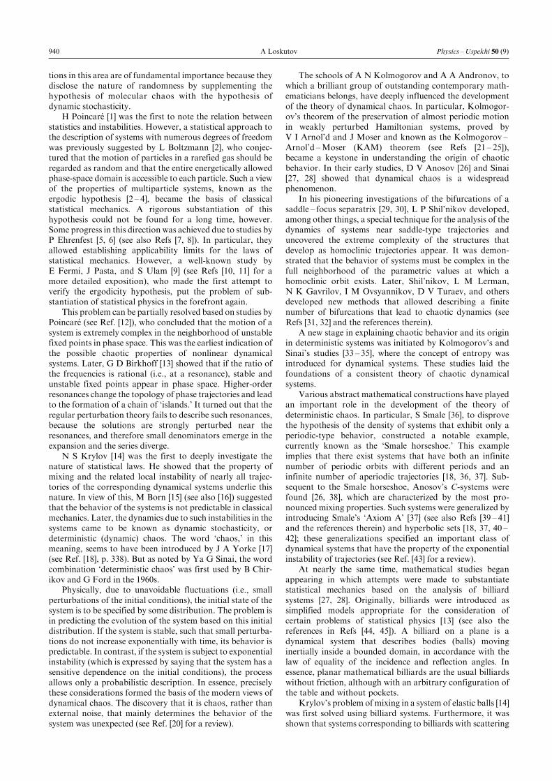
If the full energy of the pendulum, H � E, exceeds themaximum value of the potential energy, E � Erot > mgl, themomentum p is always different from zero, which leads to aninfinite increase in the angle j, i.e., to the rotation of thependulum. Energies E � Eosc < mgl correspond to oscilla-tions of the pendulum. IfE � Es � mgl, the oscillation periodtends to infinity and the motion follows the separatrixbetween the two types of motion, oscillation and rotation(Fig. 1a). The equation of the separatrix can be written asps� �2o0ml 2 cosjs=2, js � 4 arctan

�exp �o0t�

�ÿ p, wherethe plus and minus signs respectively correspond to the upperand lower branches.

In the neighborhood of the points with the coordinates�p;j� � �0; 2pk�, k � 0;�1;�2; . . . ; the family of phasecurves consists of ellipses. Such points are therefore calledelliptic. The family of trajectories near the points�p;j� � �0; p� 2pk�, k � 0;�1;�2; . . . ; is formed by hyper-bolas, and such points are called hyperbolic.

For an autonomous system with two degrees of freedom,n � 2, the integrable system in the angle ± action variables�J; a� has the topology of a two-dimensional torus (Fig. 1b).In view of the constraints o1 � o1�J1; J2� ando2 � o2�J1; J2� (if they are present), the frequencies ofgyration in circles O1 and O2 for nonlinear systems can varyfrom torus to torus. Their ratio can also vary:

o1

o2� o1�J1; J2�

o2�J1; J2� : �7�

If quantity (7) is rational,o1=o2 � k=m (a resonance), thedynamics of the system are periodic: the phase trajectorycloses after kwindings over the circleO1 andmwindings overthe circle O2. If fraction (7) is irrational, o1=o2 6� k=m, thephase trajectory covers the torus everywhere densely, and themotion of the system is called quasi-periodic, of almostperiodic.

Therefore, because J1 and J2 are arbitrary, the phase spaceis represented by two-dimensional tori, which can bevisualized in ordinary three-dimensional space as a set oftori nested in one another, with themajor andminor semiaxesspecified by the ratios J1 and J2 (Fig. 2).

a

jp

E � Erot

ÿp

p

0

E � Es

E � Eosc

b

O1

O2J1

a2J2

a1

Figure 1. (a) Phase portrait of a nonlinear pendulum and (b) a visual

representation of an integrable Hamiltonian system with two degrees of

freedom in angle ± action variables.


For integrable systems with n degrees of freedom, theirphase space is 2n-dimensional; in the angle ± action variables,it has the topology of a set of n-dimensional tori. Any possibletrajectory lies on one of them. Some trajectories may beclosed; others cover the corresponding torus everywheredensely.

A torus of dimension n5 2 with given J1; J2; . . . ; Jn iscalled resonant if the relationXn

i� 1

kioi�J1; J2; . . . ; Jn� � 0 ;

where ki are nonzero integers, holds for a set of frequencies�oi�J1; J2; . . . ; Jn�

�i � 1; 2; . . . ; n�.

3.2 Perturbed motionThe overwhelming majority of Hamiltonian equations (forsystems with n degrees of freedom) are not integrable. But aHamiltonian H � H�a ; J� can in some cases be divided intoan integrable part H0 � H0�J� and a part that is notintegrable but can be represented as a small perturbation H1

of H0:

H�a ; J� � H0 � eH1 ; �8�where H0 � H0�J�, H1 � H1�a ; J�, and e is a small para-meter. Systems whose Hamiltonians can be written in form(8) are called nearly integrable systems.

In the chosen variables a and J, the canonical equationsthat follow from Eqns (4) and (8) have the form

_Ji � ÿe qH1

qai; _ai � qH0

qJi� e

qH1

qJi; i � 1; 2; . . . ; n ;

�9�where e5 1. If e � 0, system (9) is completely integrable, andits solutions cover n-dimensional tori. We now assume thate 6� 0. How strong are then the changes in the character of theintegrable system?

4. Nonlinear resonance

The answer to the question posed in Section 3.2 essentiallydepends on the relation between the perturbing forcefrequency and the proper frequency of the system. If theproper frequency is close to the frequency of the externalforce, this results in an increase in amplitude, leading to aresonance. But for nonlinear systems with perturbation (8),the frequency depends on the amplitude, and hence thesystem falls out of resonance some time later. This reducesthe amplitude, which, in turn, changes the frequency. There-

fore, the system shortly returns to the neighborhood of theresonance. The so-called phase oscillations thus set in.

Resonances can arise not only between the system andexternal influences but also between different degrees offreedom of the system itself, which corresponds to theautonomy of the Hamiltonian H1 in Eqn (8). This is the caseof so-called internal resonances.

If the resonance is not isolated, the overlapping ofresonances results in a very complex motion in the system.Moreover, the resonances prevent finding solutions of theequations using the technique of the canonical perturbationtheory. In the perturbation theory, the original system isapproximated by a close integrable system subject to a smallperturbation, and the solution is sought as an expansion inpowers of e. The presence of resonances disrupts theconvergence of such series, because this approach implicitlyassumes that the original equations are integrable. This is notthe case in most situations, however. Even very simplesystems may not be integrable, and their dynamics may bevery complex at certain initial conditions. For example,signatures of dynamical chaos are manifested in the behaviorof a nonlinear pendulum [56, 57]. The perturbation theorycannot describe such a complex behavior, which is formallyreflected by the divergence of the series. If the initialconditions of the system correspond to regular trajectories(quasi-periodicmotion), such trajectories undergo qualitativerearrangements under the action of perturbations in theneighborhood of the resonances.

The theory of nonlinear resonance is remarkable for itsability to obtain an analytic criterion for the onset of irregularmotion in aHamiltonian system. This criterion was originallyintroduced in [58, 59]. We consider the theory of nonlinearresonance fromamore general standpoint, followingRefs [60,61] (see also Refs [54, 62]). A more complete exposition of thetheory of resonances is given in [63].

4.1 Small denominatorsWe first consider the internal resonance. We decompose thefunction H1�a ; J� [see Eqn (8)] into a Fourier series,H1�a ; J� �

Pk H

k1 �J� exp �ika�, and substitute this decom-

position in Hamilton equations (9). This yields

_Jj � ÿieXk

kjHk1 exp �ika� ;

�10�_aj � oj�J� � e

Xk

qHk1

qJjexp �ika� ; j � 1; 2; . . . ; n ;

where k is a vector with real integer components, Hk1 are the

Fourier coefficients, and oj�J� � qH0�J�=qJj.We seek a solution of perturbed system (10) in the form of

a series in powers of the small parameter e:

Jj � J�0�j �

X1s� 1

e sJ �s�j ;

�11�aj � a �0�j �

X1s� 1

e sa �s�j ; j � 1; 2; . . . ; n :

Next, using expansion (11) and Eqns (10), we select the termscontaining equal powers of e. In the zeroth approximation, wethen find _J

�0�j � 0, _a �0�j � oj�J�0��, j � 1; 2; . . . ; n. Therefore,

J�0�j � const ; a �0�j � oj�J�0��t� const : �12�

Figure 2.General structure of the phase space of an integrable system with

two degrees of freedom in the action ± angle variables.


Because

oj

ÿJ�0� � eJ�1�

� � oj

ÿJ�0�� e

Xm

qoj�J�0��qJ �0�m

J �1�m ;

we can easily obtain the first-approximation equations

_J�1�j � ÿi

Xk

kj ~Hk1 �J�0�� exp

ÿikx�J�0��t� ;

�13�_a �1�j �

Xm


J �1�m �Xk

q ~Hk1 �J�0��qJj

expÿikx�J�0��t� ;

where ~Hk1 are the values of the coefficients Hk

1 with theconstant taken into account. Equations (13) can be straight-forwardly integrated:

J�1�j � ÿ

Xk

kj ~Hk1 �J�0��kx

exp �ikxt� � const ;�14�

a �1�j � iXm


Xk

km ~Hk1 �J�0��kx�2 exp �ikxt�

ÿ iXk

q ~Hk1 �J�0��qJj

exp �ikxt�kx

:

It can easily be seen that if the condition

kx� k1o1 � k2o2 � . . .� knon � 0 �15�

(called the resonance relation) holds, terms with zero or near-zero denominators appear in Eqns (14). This leads to asubstantial increase in the corrections a �s�j and J

�s�j , which

obviously disrupts the convergence of series (11).If the resonance relation is not satisfied in first-approx-

imation equations (13), it can hold for equations of higherapproximations, s > 1. The resonance that manifests itself inthe sth order of the perturbation theory is called the order-sresonance.

We now let the perturbation H1 depend on timeperiodically (with a period T � 2p=O), i.e., H1�a ; J; t� �H1�a ; J; t� T �. A treatment similar to that used in thepreceding case yields

H1�a ; J; t� �Xk;m

Hkm1 �J� exp

�i�ka ÿmOt�� :

In this case, the Hamilton equations become

_Jj � ÿieXk;m

kjHkm1 exp

�i�ka ÿmOt�� ;

_aj � oj�J� � eXk;m

qHkm1

qJjexp

�i�ka ÿmOt��; j � 1; 2; . . . ; n :

As before, the zeroth-approximation solution is given by (12).The first-approximation equations can also be easily obtainedand integrated, yielding

J�1�j � ÿ

Xk;m

kj ~Hkm1 �J�0��

kxÿmOexp

�i�kxÿmO�t�� const ;

a �1�j � iXl

qoj�J�0��qJ �0�l

Xk;m

kl ~Hkm1 �J�0��

�kxÿmO�2 exp�i�kxÿmO�t�

ÿ iXk;m

q ~Hkm1 �J�0��qJi

exp�i�kxÿmO�t�kxÿmO

;

where ~Hkm1 are the values of Hkm

1 with the inclusion of theconstant that appears in the zeroth order. Thus, if theresonance relation kxÿmO � 0 holds, perturbation-theoryseries (11) diverge; this is the essence of the small-denomi-nator problem. To overcome this difficulty, it was suggestedthat a canonical transformation be used to pass to special(resonant) variables.

4.2 Universal HamiltonianLet the perturbationH1 be a periodic function of time with aperiod T � 2p=n and let the motion be described by theHamiltonian

H � H0�J� � eH1�a; J; t� ; �16�

where e5 1. We decompose the function H1 into a Fourierseries:

H1�a; J; t� �Xk;m

Hkm1 �J� exp

�i�kaÿmnt�� : �17�

Then Hamilton equations (9) become

_J � ÿieXk;m

kHkm1 �J� exp

�i�kaÿmnt�� ;

�18�_a � o�J� � e

Xk;m

dHkm1 �J�dJ

exp�i�kaÿmnt�� ;

where Hÿk;ÿm1 � Hk;m1

�. It can be easily verified that if the

condition

ko�J� ÿmn � 0 �19�

is satisfied in Eqns (18), then a resonance arises.To analyze the dynamics in the neighborhood of the

resonance, we isolate the resonant term in decomposition(17) and consider the behavior of the system determinedsolely by this term. We fix the triplet of numbers k0, m0, J0such that the resonance condition is satisfied exactly,

k0o�J0� � m0n ; �20�

and retain only the resonant harmonic in Eqns (18). Then,

_J � ÿiek0Hk0m0

1 �J� exp �i�k0aÿm0nt��

� iek0Hk0m0

1

� �J� exp �ÿi�k0aÿm0nt��

� 2ek01

2i

n��Hk0m0

1 �J�� exp �i�c� k0aÿm0nt��

ÿ ��Hk0m0

1 �J�� exp �ÿi�c� k0aÿm0nt��o

� 2ek0��Hk0m0

1 �J�� sin �k0aÿm0nt� c� ;

_a � o�J� � ed

dJHk0m0

1 �J� exp �i�k0aÿm0nt��

� ed

dJHk0m0

1

� �J� exp �ÿi�k0aÿm0nt��

� o�J� � 2ed

dJ

��Hk0m0

1 �J�� cos �k0aÿm0nt� c� :


We introduce the notation j � k0aÿm0nt� c andH 01 �

2jHk0m0

1 j. Then Eqns (18) can be rewritten as

_J � ek0H 01 �J� sinj ; �21�

_j � k0o�J� ÿm0n� ek0dH 0

1 �J�dJ

cosj :

Retaining only the resonant term in expansion (17), weexpress Hamiltonian (16) as

H � H0�J� � eH 01 cosj : �22�

We now assume that the quantity J is sufficiently close toJ0, such that the deviation DJ � Jÿ J0 is small. In this case,H0�J� and o�J� can be expanded into series in DJ:

H0�J� � H0�J0� � qH0

qJDJ� 1

2

q2H0

qJ 2�DJ�2 � . . . ; �23�

o�J� � o�J0� � qoqJ

DJ� 1

2

q2oqJ 2�DJ�2 � . . . : �24�

We neglect the terms of orders higher than two in Eqn (23)and higher than one in Eqn (24). In addition, we takeH 0

1 �J� atthe point J0, use equality (20), and neglect the term � e in thesecond of Eqns (21). Then system (21) and Hamiltonian (22)become

d

dtDJ � ek0H 0

1 sinj ;�25�

_j � k0do�J0�dJ

DJ ;

H � H0�J0� � o�J0�DJ� 1

2

qo�J0�qJ

�DJ�2 � eH 01 cosj : �26�

For convenience, we here use the notationH 01 � H 0

1 �J0�. Thevariables DJ and j are canonically conjugate for system (25),and system (25) itself is generated by the Hamiltonian

�H � 1

2k0

do�J0�dJ

�DJ�2 � ek0H 01 cosj ; �27�

which is called the universal Hamiltonian of nonlinearresonance [59].

The canonical transformation that allows passing fromthe system with Hamiltonian (26) to the universal Hamilto-nian of nonlinear resonance has the form

�a; J� ! k0aÿm0nt; DJ� � ; n � o�J0� ; �28��H � k0Hÿm0nDJÿ k0H0�J0� :

4.3 Width of the separatrixWe analyze expression (27) and Eqns (25). A similaritybetween �H and the Hamiltonian of the nonlinear pendulumin (5) with l � 1 can immediately be noted. Indeed, thevariable DJ plays the role of the momentum p and thequantity m � �k0 do�J0�=dJ�ÿ1 has the meaning of theeffective mass. Moreover, the substitution O 2

0 �ek 2

0H01

��do�J0�=dJ�� reduces system (25) to

�jÿ O 20 sinj � 0 : �29�

Equation (29) coincides with Eqn (6) up to a phase lag by p.

Let k0 � 1, m0 � 1 (a first-order resonance). The phaseportrait in the original variables a, J is shown in Fig. 3a. Thedouble drop-shaped curve, for a small energy E � Eosc,corresponds to local oscillations of the system. In terms ofthe pendulum analogy, this corresponds to its oscillations.The outer curve corresponds to the energy E � Erot, whichimplies rotation in the case of the pendulum. The separatrix�E � Es� separates these two qualitatively different types ofmotion.

We now pass to the coordinate system specified bytransformation (28). The resulting phase portrait is shownin Fig. 3b. We clarify this figure using the pendulumanalogy. If the pendulum rotates oppositely to therotation of the coordinate system, curves located aroundthe point O inside the minor separatrix loop correspond tosuch motion. If the pendulum corotates with the coordi-nate system, curves located outside the major separatrixloop correspond to the motion of the pendulum. Horse-shoe-shaped closed curves between the two separatrixloops correspond to oscillations of the pendulum. Theoscillations occur around the elliptic point denoted as E inFig. 3b. Both the major and minor separatrix loops passthrough the hyperbolic point H. The circle C representsthe lower equilibrium of the pendulum. For the originalsystem, the unperturbed trajectory for J � J0 correspondsto the circle C. The directions of motion are shown byarrows in Fig. 3b.

The maximum distance between the two (major andminor) separatrix loops is known as the width of thenonlinear resonance (or the separatrix width). This quantitycan easily be estimated. According to Eqn (27), we have theresonance width with respect to action

max �DJ� ��2eH 0

1

�� do�J0�dJ

��ÿ1s

�30�

and the resonance width with respect to frequency

max �Do� �� do�J0�dJ

��max �DJ� ��2eH 0

1

�� do�J0�dJ

��s

: �31�

We now find how much the above assumptions arejustified and determine the orders of magnitude of quantities(30) and (31). It follows from expression (22) that H0 � H 0

1 .But becauseH0 � J0o�J0�,

H0 � H 01 � J0o�J0� : �32�

a

a

Erot

EsEosc

J

C

O

b

O

H

C

E

Figure 3. (a) First-order nonlinear resonance in the variables a, J and (b) inthe variables specified by Eqn (28). Thin curves, phase oscillations; dot±

dashed curve, unperturbed trajectory �J � J0�; thick curve, separatrix [60].


Therefore, with (30) and (31), we obtain

max �DJ�J0

��eg

r;

max �Do�o�J0� � ��

egp

; �33�

where g � �do�J0�=dJ��J0=o�J0�� is the so-called nonli-nearity parameter. In deriving system (25), we neglectedthe term � e in Eqn (21) for _j. This can be done [seeEqns (21) and (25)] if �dH 0

1 �J0�=dJ0�e5��do�J0�=dJ��DJ, or,

in view of our estimate of the orders of magnitude, ifeH 0

1 =J0 5��do�J0�=dJ��DJ. Therefore, in accordance with (32)

and (33), we find

g4 e : �34�

In addition, we replaced H 01 �J� with H 0

1 �J0�. Thissubstitution is equivalent to the condition Jÿ J0 5 1, orDJ5 J0. As can be easily seen from relations (33), the lastinequality leads to inequality (34).

Retaining only the resonant term and neglecting thenonresonant terms is allowed if other frequencies in expan-sion (24) do not alter the dynamics qualitatively, i.e., ifo�J0�4

��do�J0�=dJ��DJ. Next, we use estimate (31) to obtainthe condition ge5 1, which is satisfied for small g and e. With(34), we therefore have

e5 g51

e: �35�

Inequality (35) is called the condition of moderate nonlinear-ity [59, 60].

Thus, the above-presented approximate theory of non-linear resonance is applicable if inequality (35) is satisfied.Therefore, there is no limit transition to the linear problem�g! 0�.

Resonance condition (20) can generally be satisfied at anyk0. In this case, all assumptions and formulas remainunchanged. But because the phase is determined by theexpression j � k0aÿ nt� c, this leads to a garland ofseparatrix loops. The number of such loops is k0. Therefore,the number of elliptic±hyperbolic pairs of points is also equalto k0 (Fig. 4).

4.4 Internal resonancesThe above description of nonlinear resonance can easily begeneralized to systems with many degrees of freedom. For

n5 2, however, resonances between the degrees of free-dom of the system itself, i.e., internal resonances, arepossible.

For clarity, we consider a system with two degrees offreedom �n � 2�. The Hamiltonian of such a system can bewritten as

H � H01�J1� �H02�J2� � eH1�J1; J2; a1; a2� ;

and the equations of motion are given by

_Jj � ÿe qH1

qaj; _aj � q

qJj�H01 �H02� � e

qH1

qJj; j � 1; 2 :

According to relation (15), internal resonance occurs if thecondition ko1�J01� ÿmo2�J02� � 0 is satisfied for certainintegers k, m and certain values of the action variables J01,J02. We retain only the resonant harmonic in the decomposi-tion

H1 �Xk;m

Hkm1 �J1; J2� exp

�i�ka1 ÿma2�

�;

expand the functions H0j and oj � dH0j=dJj, j � 1; 2, in theneighborhood of the resonance �J01; J02�, and use the aboveapproximations to obtain the equations of motion

_J1 � ekH 01 sinj ; _J2 � ÿemH 0

1 sinj ; �36�_j � k

do1�J01�dJ1

DJ1 ÿmdo2�J02�

dJ2DJ2

and the universal Hamiltonian

�H � 1

2

do1�J01�dJ1

�DJ1�2 � 1

2

do2�J02�dJ2

�DJ2�2 � eH 01 cosj ;

where we use the notation DJj � Jj ÿ J0j, j � 1; 2,H 0

1 exp �ic�� 2Hkm1 �J01; J02��2

��Hkm1 �J01; J02�

�� exp �ic�, andj � ka1 ÿma2 � c.

It can be easily seen that multiplying the first equation ofsystem (36) by m and the second by k, and adding them, weobtain an additional integral of motion mJ1 � kJ2 � const.Therefore, Eqns (36) are integrable. But we can also proceeddifferently. Differentiation of the equation for _j with respectto time yields expression (29) with

O 20 � eH 0

1

��k 2 do1�J01�dJ1

�m 2 do2�J02�dJ2

�� :If the quantities do1�J01�=dJ1 and do2�J02�=dJ2 havedifferent signs, the expression inside the modulus vanishes,i.e., an additional degeneracy is possible in the system.

For systems with more than two degrees of freedom�n5 3�, the number of additional integrals of motion islarger, but the dynamics are still governed by an equationsimilar to Eqn (29).

Thus, the ratio of frequencies plays an important rolein the analysis of nearly integrable systems: the incom-mensurability of the frequencies typically determines aquasi-periodic trajectory that densely covers the torus.But a rational frequency ratio results in the emergence ofresonances and modifies the structure of invariant sur-faces.

H

e O

Figure 4.Nonlinear resonance at k0 � 4, m0 � 1.


4.5 Overlapping of resonancesOur analysis of nonlinear resonance was based on theassumption that the quantity J [see Eqn (20)] remains fixed.In other words, we assumed that only one isolated, primarynonlinear resonance exists. But it follows from (19) that theresonance relation can also be satisfied for other Jm,m � 1; 2; . . . . In other words, there can be many primaryresonances in the system, and Eqn (20) at k0 � 1 must berewritten as o�Jm� � mn. Therefore, we can introduce thedistances between resonances: in action, dJm � Jm�1 ÿ Jm,and in frequency, dom � o�Jm�1� ÿ o�Jm�. If all Jm aresufficiently far from one another, i.e.,

dJm 4DJm ; �37�

where DJm is determined by Eqn (30), then the separatrices ofthe resonances do not intersect and no interactions betweenthe resonances occur. If the initial conditions of the system arein the domain of one of the resonances, the dynamics can bedescribed in the approximation where the effect of only thisresonance is taken into account. If the initial point is in thedomain between resonances, the system can be analyzed inthe framework of the nonresonance approximation [54, 64].

Similarly, we can formulate the condition of the absenceof frequency overlapping (interaction) of resonances:

dom 4Dom : �38�

We now assume that condition (37) or (38) is not satisfiedand the resonances are close to one another, such that thecorresponding separatrices can overlap.What happens in thiscase, known as the case of strong interaction betweenresonances?

We introduce the parameter K describing the degree ofresonance overlapping:

K � Dodo� DJ

dJ:

The overlapping parameter K was introduced by Chirikov tocharacterize the dynamics of Hamiltonian systems [58] (seealso Refs [59, 65, 66]). If the interaction is weak, i.e., K5 1,the motion in the system should be regular and the phasetrajectories should generally cover �nÿm�-dimensional torieverywhere densely. But in the case of a strong overlapping,K > 1, the dynamics of the system turn out to be very complexand different from the dynamics in the periodic and quasi-periodic regimes.

The validity of the criterion of the onset of irregularmotion based on the resonance-overlapping degree wasmany times confirmed numerically (see Refs [54, 59, 62]). Inparticular, Ref. [67] reported the origin of chaos with only tworesonances overlapping.

A specific property of this criterion is that it can relativelysimply be used to study particular systems. Indeed, it sufficesto apply the above technique in the neighborhood of only oneresonance in the approximation of the absence of all others.This makes the resonance-overlapping criterion very con-venient in practice. At the same time, it is not universallyapplicable and in some cases requires more accurate formula-tions [54, 59, 66].

4.6 Higher-order resonancesUp to this point, we have considered only primary reso-nances. However, if the perturbation e is sufficiently large, so-

called secondary resonances, which modify or even comple-tely destroy the integrals of the primary resonances, arepossible. A secondary resonance is the resonance betweenthe fundamental frequency of the unperturbed oscillation andthe frequencies of harmonics of the primary-resonance phaseoscillation. A specific feature of such a resonance is thatgarlands of separatrix loops appear near the elliptic pointinside the primary resonance.

The small denominators of the secondary resonances canbe removed as this was done for the primary resonance (seeRef. [54] for details). But such an approach has some specificfeatures when applied to secondary resonances. In particular,the width of a secondary resonance depends on e much morestrongly than that of the primary resonance [� e 1=2, seeEqns (30), (31)]. Therefore, secondary resonances are notimportant at small e (in the case of small oscillations in theprimary resonance). But if the perturbations are sufficientlystrong, secondary resonances can affect the dynamics of thesystem as strongly as the primary resonances do.

In addition to secondary resonances, higher-order reso-nances are possible in systems; they can also substantiallyaffect the motion. Thus, on the whole, the behavior of thesystem is highly involved and represents a hierarchy of verycomplex structures. We describe such a structure when weconsider the dynamics near resonance separatrices. Ouranalysis clarifies some issues related to the origin and natureof dynamical chaos.

What is the structure of resonances near elliptic andhyperbolic points? This question is directly related to thenature of chaos.

5. Elements of the Kolmogorov ±Arnol'd ±Mosertheory

A nonlinear resonance indicates that even small perturba-tions can substantially affect the dynamics of an integrableHamiltonian system. Resonances modify the topology ofphase trajectories and result in the formation of a chain ofislands in phase space. The perturbation theory cannotdescribe such resonances, because regular solutions arestrongly disturbed near them, which entails the emergence ofsmall denominators and the divergence of series. Thisproblem was already noted by PoincareÂ , who called it afundamental problem of classical mechanics. However, itwas solved only in the early 1960s, with the advent of thefamous Kolmogorov ±Arnol'd ±Moser (KAM) theory [21 ±25].

To emphasize the physical significance of the KAMtheory, we consider the problem of planetary motion aroundthe Sun in accordance with the law of gravity. If the mutualinfluence of planets is neglected, we have a completelyintegrable system: planets move in ellipses according toKepler's laws, and hence the dynamics of the system are ingeneral quasi-periodic. If the interaction of the planets istaken into account, their orbits are deformed ellipses, whichprecess slowly. The precession is maximum for Mercury. Theshift of its perihelion due to the influence of other planets 1 isestimated to be � 53200 per 100 years [68].

In principle, the interaction of planets should be takeninto account using perturbative methods. But if resonancesoccur, such techniques yield diverging series and therefore do

1 We emphasize that we consider only the Newtonian interaction.


not provide information on the dynamics of the system overlong time intervals.

This planetary problem, reducible in the general case tothe well-known N-body problem, is among the mostimportant problems that have been raised in the course ofthe development of both mathematics and physics. In 1885,King Oscar II of Sweden and Norway, at the suggestion ofG Mittag-Leffler, established a prize for solving thisproblem: ``Given a system of arbitrarily many mass pointsthat attract each other according to Newton's laws, try tofind, under the assumption that no two points ever collide, arepresentation of the coordinates of each point as a series ina variable that is some known function of time and for all ofwhose values the series converges uniformly.'' (See Ref. [69]for a more detailed exposition of this and some otherinteresting points concerning the development of celestialmechanics and nonlinear dynamics.) Thus, the principalproblem was not only to find a formal representation ofsolutions of the N-body problem in the form of series butalso to prove their convergence. It is the latter issue thatpresented the main difficulty.

Without dwelling on the history of the question, we onlynote that the prize was awarded to PoincareÂ for hisinestimable contribution to the solution of the N-bodyproblem and related fundamental problems of dynamics.

Very much time was spent to realize that the problemposed is not simple and solving it requires employing novelpowerful methods. Such methods were developed by theauthors of the KAM theory, A N Kolmogorov, V I Arnol'd,and JMoser. The KAM theory not only permits constructinga converging expansion procedure but also, most impor-tantly, gives a key to understanding the nature of the onsetof chaos. In addition, this theory and its consequences provedto be very important inmany areas of modern science, such aspure and applied mathematics, mechanics, physics, and evennumerical analysis (!).

In recent years, substantial progress has been made in theKAM theory, and it remains a field of very active research(see Refs [53, 70, 71] and the references therein). This theory ispresented in a large number of reviews and monographs (e.g.,Refs [70, 72 ± 76]). In Sections 5.1 and 5.2, we thereforedescribe only some qualitative statements of this theory anda number of its important consequences.

5.1 The Kolmogorov theoremThe famous Kolmogorov theorem (sometimes also called theKAM theorem) is at the heart of the KAM theory. It statesthat if a completely integrable system is perturbed suffi-ciently weakly, most nonresonant tori are preserved and onlyslightly deformed. In this case, the word `most' means thatall the resonant tori (corresponding to periodic motion) andpart of nonresonant tori collapse, but this set is smallcompared to the set of nonresonant tori preserved underthe perturbation.

The applicability conditions of the KAM theorem are asfollows.� The unperturbed Hamiltonian must satisfy the non-

degeneracy condition

det

�� qoi

qJk

�� det

�� q2H0

qJi qJk

�� 6� 0 ; i � 1; 2; . . . ; n ;

which means that the frequencies of the unperturbed systemare functionally independent.

� The perturbation must be smooth, i.e., the HamiltonianH1 must have a sufficient number of derivatives.� The system must be outside the neighborhood of a

resonance, i.e.,��Xj

kjoj

�� > cjkjÿr ; k � �k1; k2; . . . ; kn� ; �39�

where r depends on the number of the degrees of freedom nand the constant c is determined by the magnitude of theperturbation eH1 and the nonlinearity parameter g. We notethat the condition of moderate nonlinearity (35) can beobtained from inequality (39).

If the above conditions are satisfied, the meaning of theKAM theory is as follows. For most initial conditions, quasi-periodic dynamics are preserved in a nearly integrable system.However, there are initial conditions at which (mainlyresonant) tori existing for e � 0 break down and the motionbecomes irregular. Precisely these tori break down under theperturbation and bring the system to chaos. This is why thetheory of nonlinear resonance plays such an important role.The trajectories that originate in the region of destroyed torican freely move in the energy space, which is manifested onthe section surface as numerous randomly scattered points.Such trajectories turn out to be exponentially unstable withrespect to small perturbations.

At small e, interestingly, the tori remote from theresonance are preserved in the presence of arbitrary smoothperturbations. But the situation changes dramatically withincreasing e: the tori start breaking down and the domain ofchaos starts expanding. Ultimately, this results in an over-lapping of primary resonances and the onset of the phenom-enon known in Hamiltonian mechanics as global chaos [54].As global chaos occurs, no tori that were close to the tori inthe unperturbed problem remain in the system, althoughsome other tori can appear. The phase trajectory can movetransversally to the chaotic layers in such a system.

However, at e5 1, resonances do not overlap and thesolutions lie on weakly deformed invariant tori. There is aqualitative difference in dynamics between systems with twodegrees of freedom and those with more �n > 2� degrees offreedom.

5.2 The Arnol'd diffusionIn the case of two degrees of freedom, the phase space is four-dimensional, the energy hypersurface (or energy-level space)H � E is three-dimensional, and the invariant tori are two-dimensional. Therefore, such tori can be represented asenergy levels H � E immersed in the three-dimensionalspace of the energy level H � E (see Fig. 2). Therefore, thetori divide this space into disconnected domains. Thus, thedestroyed tori turn out to be sandwiched between the toripreserved under the perturbation. The phase trajectory thatoriginates at the location of such a destroyed torus (i.e., in thegap between two invariant tori) remains locked there forever.This means that the corresponding action variables arealmost unchanged and remain near their initial values in thecourse of motion. Therefore, for systems with two degrees offreedom satisfying the conditions of Kolmogorov's theorem,for any initial conditions, no evolution occurs and globalstability is preserved [72].

If n > 2, invariant tori no longer divide the �2nÿ 1�-dimensional energy hypersurface into nonintersecting parts.In such systems, the dynamics are quasi-periodic for most


initial conditions. But there exist initial conditions at whichthe action variables recede slowly from their initial values.This can be easily understood from the fact that, at n > 2, thedomains of destroyed tori merge, forming a cobweb. Thephase point on the hypersurface of a given energy, movingalong the threads of this cobweb, can approach any point ofthis hypersurface arbitrarily close. As investigations show,such an evolution of the action variables is random. Thisrandom walk over resonances around invariant tori is calledthe Arnol'd diffusion [54, 60, 70, 72].

Thus, small perturbations in systems with more than twodegrees of freedom not only qualitatively modify thedynamics of the system but also can change the topology ofphase trajectories, transforming them into a connected web.

A characteristic feature of the Arnol'd diffusion is itsuniversality in the sense that no critical value of theperturbation e necessary for the onset of such diffusionexists. In other words, diffusion always occurs, even atarbitrarily small e. Obviously, the diffusion rate vanishes atprogressively reduced perturbations. Therefore, for Hamil-tonian systems with n > 2 degrees of freedom, the actionvariables can evolve slowly, which corresponds to lackingglobal stability. In the general case, this evolution is fairlyslow and can be different in different parts of the phasespace.

Another peculiarity of systems in which the Arnol'ddiffusion is inherent consists in that their dynamics cannotexhibit a sudden transition to global chaos, which originatesdue to the overlapping of resonances. This is because regionswith chaotic behavior in such systems are already unified intoa web. In addition, the Arnol'd diffusion is very slowcompared to the motion of trajectories in the region of globalchaos.

The existence of diffusion trajectories was rigorouslyproved for the first time for a nonlinear Hamiltonian systemof a special form [77]. There is no proof of the merging ofchaotic trajectories into a web in the general case; however,fairly numerous examples are known in which this phenom-enon is observed (see Refs [54, 59, 78 ± 81]). The exact upperbound of the Arnol'd diffusion rate was obtained in Ref. [82](see also Ref. [53] and the references therein). Various cases ofdiffusion, the accompanying physical phenomena, andestimates of the diffusion rate for various systems arediscussed in monographs [53, 54].

We now consider the breakdown of the resonant tori andthe origin of chaos in greater detail.

6. The nature of chaos

The issue of the nature of chaotic behavior traces back tothe famous problem of intersection of separatrices indynamical systems. This phenomenon was discovered longago by PoincareÂ when he was studying the three-bodyproblem [83]. But to understand the origin of chaos insystems of classical mechanics, the well-known PoincareÂ ±Birkhoff fixed-point theorem [13, 84] should also be invoked(the mathematics of the issue can be surveyed usingmonograph [85]).

6.1 Twist mapWe consider a systemwith two degrees of freedom, n � 2, anda Hamiltonian H�q1; p1; q2; p2�, although the results pre-sented below can be generalized to the multidimensionalcase. In such a system, H is the total energy. Therefore, at a

given value of H � E, the flow is always three-dimensional.This allows considering the corresponding PoincareÂ mapinstead of the continuous evolution of the system. Such amap can easily be constructed analytically.

For an integrable system in the angle ± action variables,the phase space is a set of nested tori.Wewrite the flow on oneof them as

a1�t� � o1t� a1�0� ; a2�t� � o2t� a2�0� ;

where o1 � o1�J1; J2� � qH=qJ1 and o2 � o2�J1; J2� �qH=qJ2. Obviously, a complete revolution along the a2coordinate takes the time t2 � 2p=o2. By this time, the a1variable becomes

a1�t� t2� � a1�t� � o1t2 � a1�t� � 2po1

o2� a1�t� � 2pr�J1� :

The quantity r � o1=o2 introduced here is called the rotationnumber. Because motion occurs in the energy-level space,J2 � J2�J1;E�. Therefore, at a given E, the rotation number ris a function of J1 only.

We now assume that the surface of a section is the plane�a1; J1�, i.e., a2 � const. Then, for the intersection points xkbetween the phase trajectory and this plane (Fig. 5a), we canwrite xk �

ÿa1�t� kt2�; J1

�. Thus, solutions of the original

system on the given torus can be represented as the map P0

that takes an intersection point xk into the point xk�1 next inthe invariant circle of `radius' J1. With the notationJk � J1�t� kt2�, it is possible to write such a displacementof points as

P0 :ak�1 � ak � 2pr�Jk� ;Jk�1 � Jk :

��40�

As can be seen from (40), the rotation number r depends onthe radius of the circle in general.

If r is irrational, then the points xk fill the entire circle ask!1. If r � l=m is rational, the points xk map into oneanother successively, eachm steps (Fig. 5b). Therefore, if thisrepresentation is used, we can speak of nonresonant andresonant circles.

As we pass from one circle to another, the rotationnumber changes. To be specific, we assume that r�J�increases with increasing J. Then, as the origin of coordinatesrecedes, the angle through which the circle is rotated increaseson average. This results in a twist of the radial line of pointsunder the action of P0. For this reason, transformation (40) is

b

xk�2xk�1

xkJ

aa2

a1J1

J2

xk

a

Figure 5. A system with two degrees of freedom (a) and its PoincareÂ

map (b).


called the rotation map (or sometimes the twist map). In thegeneral form, it can be written as

P0�C� � C :

An important property of themapP0 is that it is conservative.We now consider perturbed system (9) with Hamiltonian

(8). In the PoincareÂ section, taking the perturbation intoaccount corresponds to adding new terms to the twist map:

Pe :ak�1 � ak � 2pr�Jk� � ef �Jk; ak� ;Jk�1 � Jk � eg�Jk; ak� ;

(�41�

where f and g are functions periodic in a. As before, thetransformation Pe must preserve the area; otherwise, invar-iant circles do not exist, as a rule. According to the KAMtheory, under a small perturbation, e5 1, most circles withirrational r are preserved, being only slightly deformed. Weconsider the behavior of the circles in the domain of rational,or resonant, values r � l=m, for which relation (39) is notvalid. It is in this domain, as we already noted, chaotic motionoriginates.

6.2 Fixed-point theoremWe temporarily return to the integrable case. At r�J� � l=m,any point of the circle returns to its initial position after msteps, i.e., it is periodic with the periodm. We let C denote thisresonant circle and consider two nonresonant invariantcircles C� and Cÿ on both sides of C (Fig. 6a). Because r�J�increases with J (see Section 6.1.), the irrational rotationnumbers of such circles satisfy the respective inequalitiesr > l=m and r < l=m. After applying the map P0 m times(with the iterated map denoted by Pm

0 ), the points of the circleC� are rotated through an angle larger than 2p and the pointsof the circle Cÿ through an angle smaller than 2p. It thereforeappears that relative to C, the mapwinds C� counterclockwiseand Cÿ clockwise (Fig. 6a).

We now consider perturbed map (41). According to theKAM theory, the circles C� and Cÿ are preserved and onlyslightly deformed under the perturbation. Such closed circles,respectively denoted as C�e and Cÿe , are invariant under thetransformation Pe:

Pe�C�e � � C�e ; Pe�Cÿe � � Cÿe :

We assume that the parameter e is sufficiently small for therelative rotation of C�e and Cÿe to be preserved under theaction of Pm

e . Then, at any radius a � const between thecurves C�e and Cÿe , a point Jp�a; e� can be found such that the

map Pme rotates its angular coordinates exactly through 2p.

Therefore, the angular coordinates of this point are preservedunder Pm

e . At each radius issuing from the center, only onesuch point is located. Because the perturbation Pe is smooth,these points Jp�a; e� form a certain closed curve Ge (Fig. 6b)that shrinks to C as e! 0. The curve Ge is not invariant underPe. The action of Pm

e amounts to radially shifting each pointof Ge. Thus, a new curve Pm

e �Ge� is formed instead of Ge

(Fig. 7a).Next, we recall that the mapPe is conservative. Therefore,

both curves Ge and Pme �Ge� must confine equal areas. Hence,

the curve Pme �Ge� can be neither inside nor outside the curve

Ge. Therefore, these curves must in general intersect 2 at aneven number of points (Fig. 7a). In turn, each of theseintersection points is fixed under the perturbed transforma-tion Pm

e .This is the principal meaning of the PoincareÂ ± Birkhoff

fixed-point theorem [13, 84], according to which theperturbed twist map (41) with the rotation number r � l=mhas 2im, i � 1; 2; . . . ; fixed points. Thus, as the resonant circleis perturbed (we recall that any point of this circle is fixedunder the transformation Pm

0 ), only an even number 2im offixed points is preserved.

We consider one of the points, p, of intersection betweenthe curves Ge and Pm

e �Ge� (Fig. 7a). It is fixed under the mapPme . The transformation Pe acting on p generates a sequence

of points p;Pep;P2e p; . . . ;Pmÿ1

e p; after m iterations, the pointp returns to its initial position. On the other hand, each ofthem is a fixed point for Pm

e . Thus, there are m fixed pointsassociated with the original point p. Because the curvesGe andPme �Ge� intersect at an even number of points, we have a total

of 2im fixed points.

6.3 Elliptic and hyperbolic pointsA detailed consideration of the map Pe in the neighborhoodof various points p reveals the following qualitative differ-ence. Points neighboring some points p remain near them andappear to rotate around them, while points located near otherp tend to leave their neighborhood. Points of these two sortsalternate (Fig. 7b). Similar motion is observed in the phasespace of a nonlinear pendulum (see Section 3.1). For thisreason, such points are respectively called elliptic andhyperbolic. Elliptic points are surrounded by a family ofclosed trajectories that are invariant under Pm

e and form`islands'; hyperbolic points are connected by separatrices.This pattern is typical of weakly perturbed nonlinear systems,and it always emerges near a resonance.

Each island satisfies the KAM theory. Therefore, mostnonresonant circles are preserved. But resonances are also

C

Cÿ

C� a C�e

Cÿe

Jp

Ge

b

Figure 6. (a) Invariant circles C, C�, and Cÿ of the unperturbed twist map

P0 for r � l=m, r > l=m, and r < l=m, respectively. (b) The result of the

action of the perturbation Pe.

aC�e

Ge

Pme �Ge�

Cÿe

bC�e

Ge

Pme �Ge�

Cÿep

Figure 7. (a) Transformation of the curve Ge into the curve Pme �Ge� under

the action of the map Pe and (b) elliptic and hyperbolic points arising in

this case.

2 We do not consider the exceptional case of tangency.


present here. According to the PoincareÂ ± Birkhoff fixed-point theorem, a sequence of alternating elliptic and hyper-bolic points appears in the neighborhood of each resonance,although on a smaller scale (Fig. 8). In turn, an island neareach of these elliptic points reproduces the entire pattern inminiature. Closed curves in the neighborhood of ellipticpoints correspond to minor tori. According to the KAMtheory, some of theseminor tori are preserved; others collapseinto smaller ones due to higher-order resonances, and so on,to infinity. Thus, the resonance results in a very complexpattern, which repeats itself on progressively smaller scales,thus being, in a certain sense, self-similar.

Following Refs [72, 86], we now consider the phenomenain the neighborhood of hyperbolic points. Each of thesepoints is characterized by four invariant directions (orseparatrix branches): two stable ones �w s�, which enter thehyperbolic pointH, and two unstable ones �w u�, which issuefrom H (Fig. 9). Because we are considering the PoincareÂmap, these curves correspond to surfaces, or invariantmanifolds, either stable �W s� or unstable �W u�, in theoriginal phase space.

The oscillation period is infinite at the separatrix. There-fore, if some point q belongs to the stable branch w s, itapproaches H exponentially slowly under the action of themap P, i.e.,

limk!1

Pkq! H :

But if q 2 w u, it leaves the neighborhood of H exponentiallyslowly, i.e.,

limk!1

Pÿkq! H :

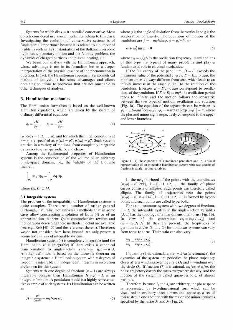
6.4 Splitting of separatrices. Homoclinic tanglesIn the case of an integrable system, stable and unstablemanifolds of hyperbolic points can be connected to one

another, forming smooth structures. In a PoincareÂ map,such a structure appears as a smooth transition from anunstable to a stable separatrix branch. Separatrix branchescan either close to the same hyperbolic point (Fig. 10a) orconnect several such points, forming garlands (Fig. 10b). Inthe first case, a stable �w s� and an unstable �wu� separatrixbranch forms a loop. This loop, known as a homoclinic loop,is a doubly asymptotic trajectory with the property that anypoint q on such a loop always approachesH, i.e.,

limk!�1

Pkq! H :

An elliptic point exists inside the homoclinic curve.In the second case, the curves consisting of stable and

unstable separatrix branches are called heteroclinic trajec-tories. The motion along such trajectories implies exponen-tially slow recession from one hyperbolic point and approachto another.

If a perturbation is present, the separatrix branches nolonger form smooth homoclinic and heteroclinic junctionsbut can intersect. The point of the intersection of a stable andan unstable separatrix branches of the same resonance iscalled a homoclinic point. If a stable and an unstable branchof different hyperbolic points (resonances) intersect, aheteroclinic point appears. We now consider how such pointsevolve under the action of the map Pe.

Let q be a homoclinic point and q 0 2 w s and q 00 2 w u be itsneighboring points (Fig. 11a). Under the action of Pe, thepoints q 0 and q 00 must be mapped into the points Peq

0 andPeq

00. Where should we find the point Peq into which q ismapped by Pe? As can be seen from Fig. 11a, taking thedirections of motion in the stable and unstable branches intoaccount, q is located before the points q 0 and q 00. Therefore,becausePe is continuous, this point must be taken into a pointthat is also located before the points Peq

0 and Peq00. This

means that a new intersection, i.e., a new homoclinic pointPeq, must arise (Fig. 11b).

Figure 8.Destruction of tori with rational frequency ratios and the origin

of a self-similar structure.

w s

wu

w s

wu

H

a

b

W u

W s

w s

w u

w s

w u

H

Figure 9. Stable �w s� and unstable �w u� directions of a hyperbolic pointHin the PoincareÂ map (a) and the corresponding manifolds W s and W u in

the phase space (b).

H1

b

H3

H2

H

a

Figure 10. A homoclinic (a) and a heteroclinic (b) trajectory formed by

separatrix branches.

Peq00

q 00

q 0

q

w s

wu

H

Peq0

a

Peq00q 00

q 0q

w s

wu

H

Peq0

Peq

P 2e q

b

Figure 11.Mapof neighboring points q 0 and q 00 and the formation of loops

from separatrices.


In other words, because the branches w s and w u areinvariant, we should remain at both separatrix branchesunder the action of the map. Therefore, a new intersectionpoint Peq emerges, and a loop forms between the points q andPeq.

By similar considerations, we can easily find that the pointPeq is mapped into the point P 2

e q, forming another loop(Fig. 11b). Because the new point P 2

e q is closer to thehyperbolic point H, the distance between P 2

e q and Peq isshorter than the distance between Peq and q. We recall thatthe conservation of phase volume is a property of the map Pe.Thismeans that the areas confined by the loops between q andPeq and between Peq and P 2

e q must be equal. Therefore, thesecond loop is more stretched and curved than the first one.

Continuing our considerations leads us to the conclusionthat an infinite number of intersections of separatrix brancheseventually arise, which become progressively closer, and theloops themselves become longer and thinner (Fig. 12a). Thestable separatrix branch w s behaves similarly (Fig. 12b). Thiscan easily be understood if we move along w s in the oppositedirection. Thus, the pattern in the neighborhood of hyper-bolic points is on the whole extremely complex (Fig. 12c).

For heteroclinic trajectories, the intersection of separa-trices results in the formation of somewhat different struc-tures. The unstable branch w u issuing from the hyperbolicpoint H1 oscillates in approaching a hyperbolic point H2

located on the right. In contrast, the stable point w s oscillatesin receding from H1 (Fig. 13). The stable and unstablebranches located in the bottom part of the figure (not shownin full) behave similarly.

Thus, due to a perturbation introduced into the integrablesystem, the separatrices are no longer smooth, as in Fig. 10,but split in an intricate manner. This phenomenon is termedthe splitting of separatrices. The structures formed byseparatrix branches in the domain of hyperbolic points arecalled homoclinic and heteroclinic tangles. It is such complexbehavior of separatrices that gives rise to chaos in determi-

nistic systems. Invariant tori cannot exist in the domain ofhomoclinic tangles. There, the systems are not integrable,exhibit the property of the exponential instability of trajec-tories under small perturbations, and therefore behavechaotically. However, at some different initial conditionsfrom the neighborhood of the surviving tori, the dynamicsof the system are regular.

We can now imagine the entire pattern arising in phasespace and in the PoincareÂ section of the set of invariant tori.The destruction of resonant circles under perturbations isaccompanied by the occurrence of 2im hyperbolic and ellipticpoints. In the neighborhood of each elliptic point, a family ofclosed invariant curves is present, and some of them are alsodestroyed by the perturbation. This leads to a smaller chain ofelliptic and hyperbolic points. In the neighborhood of eachhyperbolic point, the separatrices split, their tangles appear,etc. (Fig. 14a).

However, all this occurs not in the PoincareÂ section but inthe phase space formed by a set of tori. Thus, the generalpattern of motion of the phase trajectories turns out to behighly involved (Fig. 14b). This structure repeats itself onprogressively smaller scales and is typical of nearly integrablesystems.

As the perturbation increases, some nonresonant circlesalso break down. But if the perturbation H1 is small, chaotictrajectories exist only in the phase-space domain bounded byinvariant curves.

An elementary exposition of the foundations of thetheory, the questions concerning the physical aspects ofseparatrix intersection, and a historical background aregiven in monograph [69]. A rigorous presentation of relatedtopics is made in Refs [53, 72, 86, 88]. The fixed-pointtheorem, its qualitative description, and some applicationscan be found in book [13]. Mathematical approaches to theproblem of separatrix intersection are presented in Refs [32,63, 71, 88 ± 90].

7. The Mel'nikov method

The distance between separatrices can be estimated analyti-cally and the conditions for the onset of homoclinic andheteroclinic chaos can be obtained using the Mel'nikov'stheory [91] (see also Refs [54, 63, 88, 89]).

To simplify the presentation, we consider a two-dimen-sional autonomous system with a periodic external perturba-tion

_x � f0�x� � ef1�x; t� ; �42�

[where x � �x1; x2�, f0 � � f01; f02�, f1 � � f11; f12�, andf1�x; t� � f1�x; t� T �] that has a unique hyperbolic

a b c

Figure 12.Homoclinic tangles in the neighborhood of a hyperbolic point.

w s

H1 H2w s

w s

w s

w swu

wu

wu

wu

wu

Figure 13. Formation of heteroclinic tangles.

ba

Figure 14. Structure of the phase space of perturbed Hamiltonian systems

with two degrees of freedom: (a) in the PoincareÂ map and (b) in the phase

space [87].


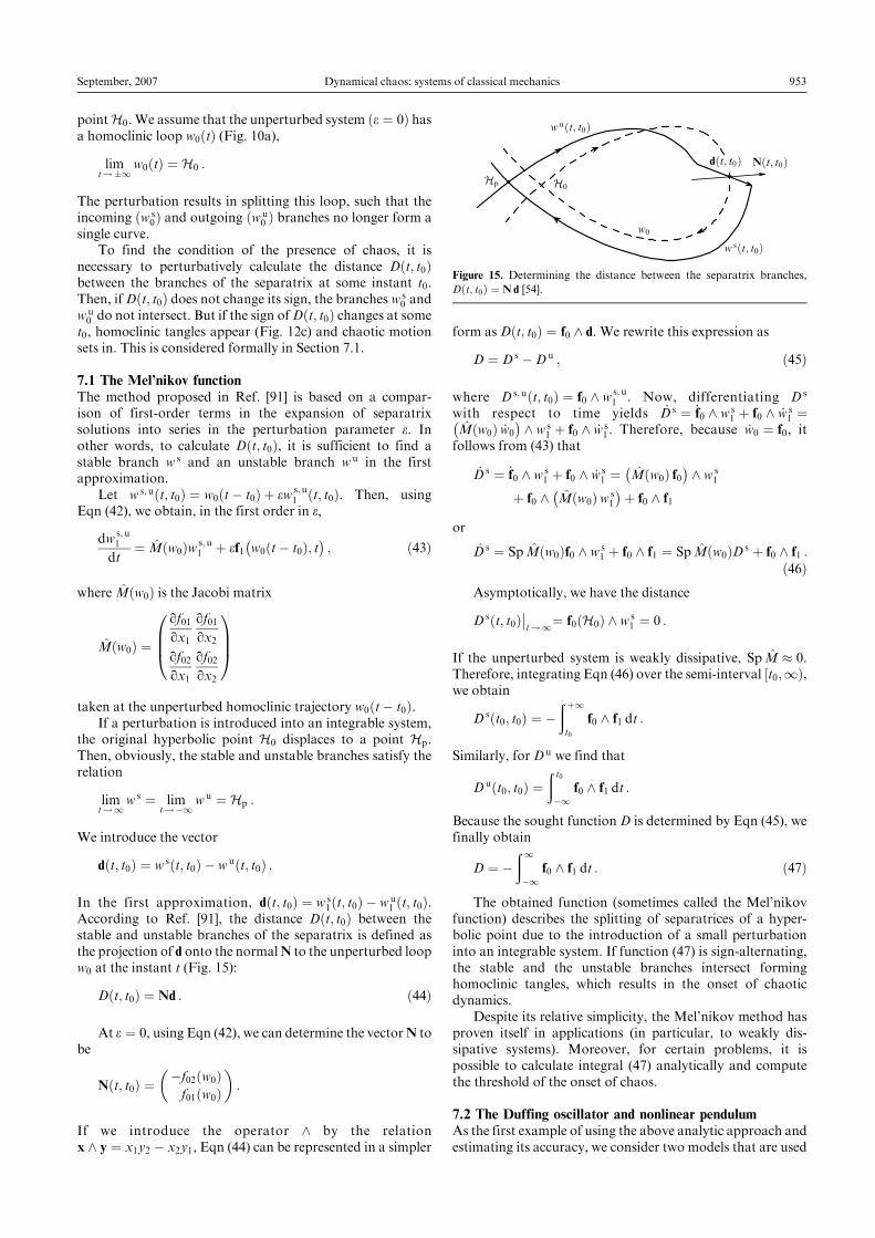
pointH0. We assume that the unperturbed system �e � 0� hasa homoclinic loop w0�t� (Fig. 10a),

limt!�1

w0�t� � H0 :

The perturbation results in splitting this loop, such that theincoming �w s

0� and outgoing �w u0 � branches no longer form a

single curve.To find the condition of the presence of chaos, it is

necessary to perturbatively calculate the distance D�t; t0�between the branches of the separatrix at some instant t0.Then, ifD�t; t0� does not change its sign, the branches w s

0 andw u0 do not intersect. But if the sign ofD�t; t0� changes at some

t0, homoclinic tangles appear (Fig. 12c) and chaotic motionsets in. This is considered formally in Section 7.1.

7.1 The Mel'nikov functionThe method proposed in Ref. [91] is based on a compar-ison of first-order terms in the expansion of separatrixsolutions into series in the perturbation parameter e. Inother words, to calculate D�t; t0�, it is sufficient to find astable branch w s and an unstable branch w u in the firstapproximation.

Let w s; u�t; t0� � w0�tÿ t0� � ew s; u1 �t; t0�. Then, using

Eqn (42), we obtain, in the first order in e,

dw s; u1

dt� M̂�w0�w s; u

1 � ef1ÿw0�tÿ t0�; t

�; �43�

where M̂�w0� is the Jacobi matrix

M̂�w0� �qf01qx1

qf01qx2

qf02qx1

qf02qx2

0BB@1CCA

taken at the unperturbed homoclinic trajectory w0�tÿ t0�.If a perturbation is introduced into an integrable system,

the original hyperbolic point H0 displaces to a point Hp.Then, obviously, the stable and unstable branches satisfy therelation

limt!1w s � lim

t!ÿ1w u � Hp :

We introduce the vector

d�t; t0� � w s�t; t0� ÿ w u�t; t0� :

In the first approximation, d�t; t0� � w s1�t; t0� ÿ w u

1 �t; t0�.According to Ref. [91], the distance D�t; t0� between thestable and unstable branches of the separatrix is defined asthe projection of d onto the normalN to the unperturbed loopw0 at the instant t (Fig. 15):

D�t; t0� � Nd : �44�

At e � 0, using Eqn (42), we can determine the vectorN tobe

N�t; t0� � ÿf02�w0�f01�w0�

� �:

If we introduce the operator ^ by the relationx ^ y � x1y2 ÿ x2y1, Eqn (44) can be represented in a simpler

form as D�t; t0� � f0 ^ d. We rewrite this expression as

D � D s ÿD u ; �45�

where D s; u�t; t0� � f0 ^ w s;u1 . Now, differentiating D s

with respect to time yields _D s � _f0 ^ w s1 � f0 ^ _w s

1 �ÿM̂�w0� _w0

� ^ w s1 � f0 ^ _w s

1. Therefore, because _w0 � f0, itfollows from (43) that

_D s � _f0 ^ w s1 � f0 ^ _w s

1 �ÿM̂�w0� f0

� ^ w s1

� f0 ^ÿM̂�w0�w s

1

�� f0 ^ f1

or

_D s � Sp M̂�w0�f0 ^ w s1 � f0 ^ f1 � Sp M̂�w0�D s � f0 ^ f1 :

�46�Asymptotically, we have the distance

D s�t; t0��t!1� f0�H0� ^ w s

1 � 0 :

If the unperturbed system is weakly dissipative, Sp M̂ � 0.Therefore, integrating Eqn (46) over the semi-interval �t0;1�,we obtain

D s�t0; t0� � ÿ� �1t0

f0 ^ f1 dt :

Similarly, for D u we find that

D u�t0; t0� �� t0

ÿ1f0 ^ f1 dt :

Because the sought function D is determined by Eqn (45), wefinally obtain

D � ÿ�1ÿ1

f0 ^ f1 dt : �47�

The obtained function (sometimes called the Mel'nikovfunction) describes the splitting of separatrices of a hyper-bolic point due to the introduction of a small perturbationinto an integrable system. If function (47) is sign-alternating,the stable and the unstable branches intersect forminghomoclinic tangles, which results in the onset of chaoticdynamics.

Despite its relative simplicity, the Mel'nikov method hasproven itself in applications (in particular, to weakly dis-sipative systems). Moreover, for certain problems, it ispossible to calculate integral (47) analytically and computethe threshold of the onset of chaos.

7.2 The Duffing oscillator and nonlinear pendulumAs the first example of using the above analytic approach andestimating its accuracy, we consider two models that are used

w0

H0Hp

wu�t; t0�

w s�t; t0�

N�t; t0�d�t; t0�

Figure 15. Determining the distance between the separatrix branches,

D�t; t0� � Nd [54].


to test various applications of the methods of analytictreatment of nonlinear systems: the Duffing oscillator [92]and a nonlinear pendulum with dissipation and periodicexcitation.

The Duffing oscillator is a system with two stableequilibrium states divided by a single separatrix and withexcitation. The equation describing such a system is called theDuffing equation:

�x� d _xÿ x� x 3 � g cosot : �48�

Equation (48) has been comprehensively studied, on the onehand, numerically and analytically and, on the other hand,experimentally (see, e.g., Refs [88, 93 ± 95] and the referencestherein).

At d � 0, Eqn (48) always has chaotic solutions near theseparatrix, which are bounded by invariant curves. In thedissipative case, no such curves exist, and hence, with thepassage of time, a chaotic trajectory finds its way to theattraction region of a stable focus or limit cycle. In this case,transient chaos is observed in the system.

The Mel'nikov function for Eqn (48) can be estimatedwithout difficulty (see Ref. [96]). We rewrite Eqn (46) ina different form, _x � y, _y � xÿ x 3 ÿ dy� g cosot. Theunperturbed Hamiltonian is then given by H0 �y 2=2ÿ x 2=2� x 4=4. The equations of motion at the separa-trix can be written as [96]

x0�t� ��2p

cosh t; y0�t� � ÿ

��2p sinh t

cosh2 t:

Using these relations, we next find f0 ^ f1 � y0�g cosotÿ dy0�.The integral of this function can be analytically calculated as

D�t0� ��2p

pgosinot0

cosh �po=2� �4

3d :

Hence, the condition of intersection of separatrices can bewritten as

d < dc � 3��2p

pgo4 cosh �po=2� : �49�

A generalized Duffing equation is also often considered; itdescribes an oscillator with a parametrically perturbed cubicterm,

�x� d _xÿ x� b�1� Z cosOt�x 3 � g cosot ; �50�where Z5 1 is the amplitude and O is the frequency of theparametric perturbation. This equation is interesting becauseit has two excitation frequencies, o and O.

TheMel'nikov function for Eqn (50) can be written as (seeRef. [97])

D�t0� � ÿA sinot0 � B sinOt0 � C ;

where

A � pkgo sechpo2;

B � 1

24pbZk 4O 2�4� O 2� cosech pO

2;

C � 2

3k 2d ; k �

��2

b

s:

If o � O, the values of d at which D can change sign can beexplicitly written as

d < dc � 3

2k 2jBÿ Aj : �51�

For o 6� O, we must additionally consider the cases ofcommensurate and incommensurate frequencies o and O. Inthe former case,

d < dc � 3�A� B�2k 2

:

For incommensurate frequencies (see Ref. [98]),

3

2k 2jAÿ Bj < dc <

3

2k 2�A� B� :

For a nonlinear pendulum that obeys the equation�x� a _x� sin x � g cosot, the Mel'nikov function can alsobe calculated analytically [56, 57],

D�t0� � ÿ4aB�1

2; 1

�� 2pg cosot0

cosh po=2;

where B�r; s� is the Euler b function. Based on this, thethreshold of the onset of chaotic motion can also bedetermined.

As found in Refs [56, 96, 98], the obtained analytic resultsagree very well with numerical estimates based on calcula-tions of the maximal Lyapunov exponent. For example, atb � 8, g � 0:114, Z � 0:03, and o � O � 1:1 [see Eqn (50)],we obtain dc � 0:3798 from (51). A numerical analysis yieldsdc � 0:378 as the threshold of the onset of chaos.

Thus, in some cases, the Mel'nikov method allowsanalytically determining the threshold of the onset of chaos,in particular, for multidimensional systems [99]. We empha-size, however, that this is a local criterion that can be used inthe neighborhood of unperturbed separatrix loops.

8. Principal properties of chaotic systems

We now describe important properties inherent in chaoticsystems: unpredictability, irreversibility, and decay of corre-lations. However, we start by introducing the concept ofmixing.

8.1 Ergodicity and mixingWe assume that the trajectories of a dynamical system arelocalized in a certain bounded domain D of the phase space.The motion of the dynamical system is said to be ergodic (orthe dynamical system is called ergodic) if, for an arbitraryintegrable function h�x�, at almost all initial conditions x0, thetemporal and phase averages of h�x� coincide:

limT!1

1

T

� T

0

h�F tx0� dt ��D�

h�x� dm ;�52�

m�D� ��D�

dm � 1 :

Thus, if the motion of a conservative system is ergodic, aphase trajectory, with the passage of time, uniformly anddensely covers the hypersurface specified by all integrals ofmotion in the n-dimensional phase space. A characteristicproperty of the ergodic motion of aHamiltonian system is theinvariance of the shape of a small domain. As time passes,


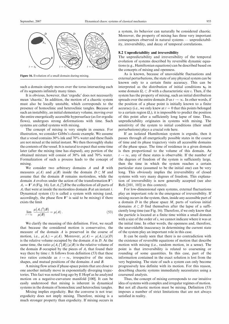
such a domain simply moves over the torus intersecting eachof its segments infinitely many times.

It is obvious, however, that `ergodic' does not necessarilymean `chaotic.' In addition, the motion of a chaotic systemmust also be locally unstable, which corresponds to thepresence of homoclinic and heteroclinic tangles. Because ofsuch an instability, an initial elementary volume, moving overthe entire energetically accessible hypersurface (as for ergodicflows), undergoes strong deformations with time. Suchsystems are called systems with mixing.

The concept of mixing is very simple in essence. Forillustration, we consider Gibbs's classic example. We assumethat a vessel contains 30% ink and 70%water and these fluidsare not mixed at the initial instant. We then thoroughly shakethe contents of the vessel. It is natural to expect that some timelater (after the mixing time has elapsed), any portion of theobtained mixture will consist of 30% ink and 70% water.Formalization of such a process leads to the concept ofmixing.

We consider two arbitrary domains A and B withmeasures m�A� and m�B� inside the domain D �M andassume that the domain B remains motionless, while thedomain A evolves under the action of the transformation F t:At � F tA (Fig. 16). Let At

TB be the collection of all parts of

At that were at inside the motionless domain B at an instant t.Dynamical system (1) is called a system with mixing (and,accordingly, the phase flow F t is said to be mixing) if thereexists the limit

limt!1

mÿAt

TB�

m�B� � m�A� : �53�

We clarify the meaning of this definition. First, we recallthat because the considered motion is conservative, themeasure of the domain A is preserved in the course ofmotion, i.e., m�At� � m�A�. Moreover, m�A� � m�At�=m�D�is the relative volume occupied by the domain A in D. At thesame time, the ratio m

ÿAt

TB�=m�B� is the relative volume of

the domain B occupied by the pieces of At that found theirway there by time t. It follows from definition (53) that thesetwo ratios coincide as t!1, irrespective of the sizes,shapes, and mutual positions of the domains A and B.

Amixing flow arises if phase-space points that are close toone another initially move in exponentially diverging trajec-tories. This fact was noted long ago by EHopf as he analyzedmotion on a negative-curvature manifold [100]. It can beeasily understood that mixing is inherent in dynamicalsystems in the domain of homoclinic and heteroclinic tangles.

Mixing implies ergodicity. But the converse is not true:ergodicity does not imply mixing. Therefore, mixing is amuch stronger property than ergodicity. If mixing occurs in

a system, its behavior can naturally be considered chaotic.Moreover, the property of mixing has three very importantconsequences observed in natural systems Ð unpredictabil-ity, irreversibility, and decay of temporal correlations.

8.2 Unpredictability and irreversibilityThe unpredictability and irreversibility of the temporalevolution of systems described by reversible dynamic equa-tions (e.g., Hamiltonian equations) can be described based onthe concepts of mixing and openness.

As is known, because of unavoidable fluctuations andexternal perturbations, the state of any physical system can beknown only to a certain finite accuracy. This can beinterpreted as the distribution of initial conditions x0 insome domain Oe � D with a characteristic size e. Then, if thesystem has the property of mixing, such an initial distributionspreads over the entire domainD as t!1. In other words, ifthe position of a phase point is initially known to a finiteaccuracy (i.e., we only knew at t � 0 that this points belongedto a certain region Oe), it is impossible to predict the positionof this point after a sufficiently long lapse of time. Thus,unpredictability originates in systems with mixing. Thesensitivity of the system to initial conditions (their smallperturbations) plays a crucial role here.

If an isolated Hamiltonian system is ergodic, then itpasses through all energetically possible states in the courseof time and its phase trajectory visits all accessible domainsof the phase space. The time of residence in a given domainis then proportional to the volume of this domain. Ast!1, any of these states is observable. If the number ofthe degrees of freedom of the system is sufficiently large,then the time in which the system reaches a certainparticular state (assumed to be the initial one) can be verylong. This obviously implies the irreversibility of closedsystems with very many degrees of freedom. This explana-tion of irreversibility is now generally accepted (see alsoRefs [101, 103] in this context).

For low-dimensional open systems, external fluctuationsplay an important role in the emergence of irreversibility. Ifmixing occurs in the system, then, inside any accessible part ofa domain D in the phase space M, parts of various initialdomains A � D find themselves after the lapse of a suffi-ciently long time (see Fig. 16). Therefore, if we only know thatthe particle is located at a finite time within a small domainwith a size of the order of e, we cannot indicate where it was atthe initial time. In other words, the openness and, therefore,the unavoidable inaccuracy in determining the current stateof the system play an important role in this case.

It can be easily seen that there is no contradiction withthe existence of reversible equations of motion that describemotion with mixing (i.e., random motion, in a sense). Thepoint is that irreversibility is related to coarsening orrounding of some quantities. In this case, part of theinformation contained in the exact solution is lost from thevery beginning. The state of such a system can only becomeprogressively less definite with its motion. For this reason,describing chaotic systems immediately necessitates using acoarsened analysis.

Thus, the concept of mixing corresponds to our intuitiveidea of systemswith complex and irregular regimes ofmotion.But not all chaotic motion must be mixing. Definition (53)imposes a number of strict limitations that are not alwayssatisfied in reality.

D

B BB

t � t0 t � t1 t � t2

D D

At2At1At0

Figure 16. Evolution of a small domain during mixing.


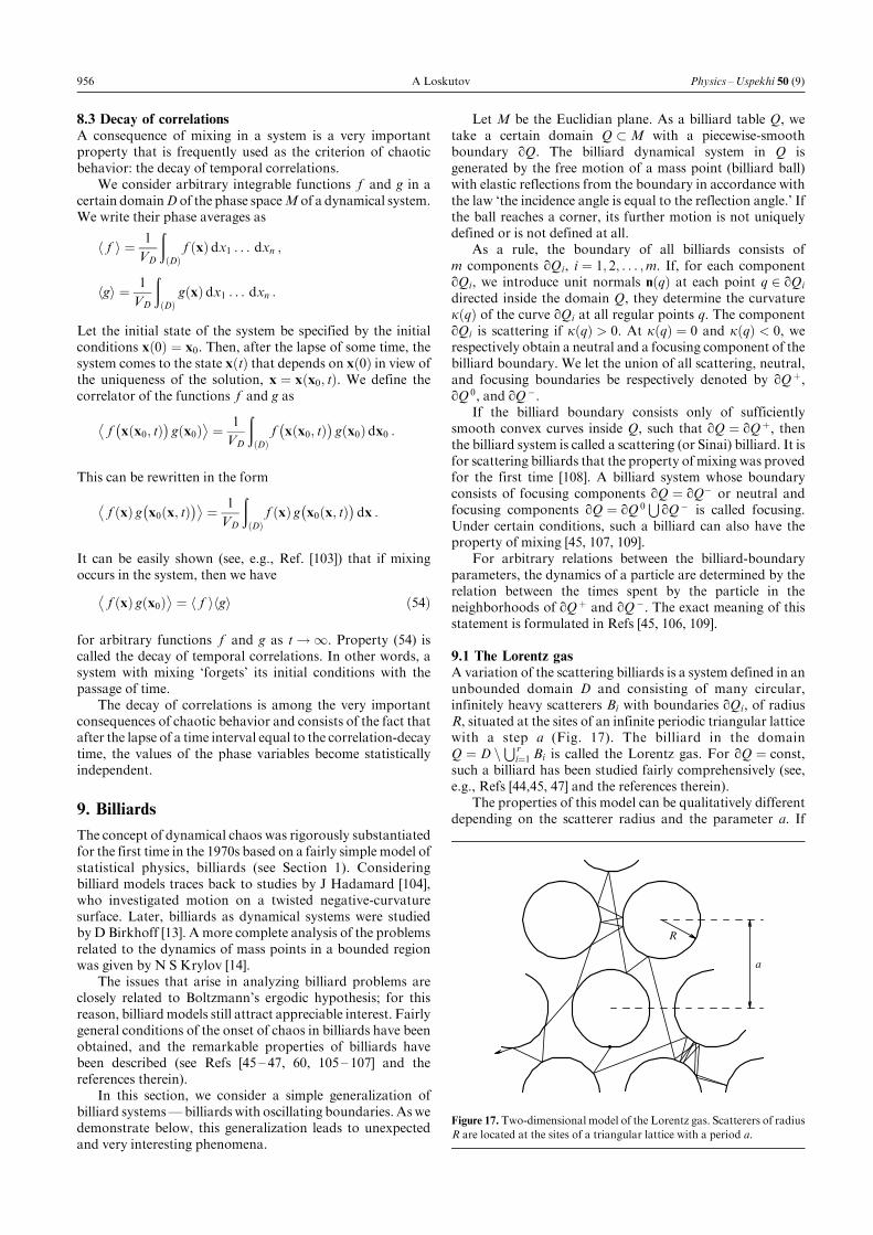
8.3 Decay of correlationsA consequence of mixing in a system is a very importantproperty that is frequently used as the criterion of chaoticbehavior: the decay of temporal correlations.

We consider arbitrary integrable functions f and g in acertain domainD of the phase spaceM of a dynamical system.We write their phase averages as

h f i � 1

VD

��D�

f �x� dx1 . . . dxn ;

hgi � 1

VD

��D�

g�x� dx1 . . . dxn :

Let the initial state of the system be specified by the initialconditions x�0� � x0. Then, after the lapse of some time, thesystem comes to the state x�t� that depends on x�0� in view ofthe uniqueness of the solution, x � x�x0; t�. We define thecorrelator of the functions f and g as

fÿx�x0; t�

�g�x0�

� � 1

VD

��D�

fÿx�x0; t�

�g�x0� dx0 :

This can be rewritten in the formf �x� gÿx0�x; t�� 1

VD

��D�

f �x� gÿx0�x; t�� dx :It can be easily shown (see, e.g., Ref. [103]) that if mixingoccurs in the system, then we have

f �x� g�x0�� h f ihgi �54�

for arbitrary functions f and g as t!1. Property (54) iscalled the decay of temporal correlations. In other words, asystem with mixing `forgets' its initial conditions with thepassage of time.

The decay of correlations is among the very importantconsequences of chaotic behavior and consists of the fact thatafter the lapse of a time interval equal to the correlation-decaytime, the values of the phase variables become statisticallyindependent.

9. Billiards

The concept of dynamical chaos was rigorously substantiatedfor the first time in the 1970s based on a fairly simple model ofstatistical physics, billiards (see Section 1). Consideringbilliard models traces back to studies by J Hadamard [104],who investigated motion on a twisted negative-curvaturesurface. Later, billiards as dynamical systems were studiedby D Birkhoff [13]. Amore complete analysis of the problemsrelated to the dynamics of mass points in a bounded regionwas given by N S Krylov [14].

The issues that arise in analyzing billiard problems areclosely related to Boltzmann's ergodic hypothesis; for thisreason, billiardmodels still attract appreciable interest. Fairlygeneral conditions of the onset of chaos in billiards have beenobtained, and the remarkable properties of billiards havebeen described (see Refs [45 ± 47, 60, 105 ± 107] and thereferences therein).

In this section, we consider a simple generalization ofbilliard systemsÐbilliards with oscillating boundaries. Aswedemonstrate below, this generalization leads to unexpectedand very interesting phenomena.

Let M be the Euclidian plane. As a billiard table Q, wetake a certain domain Q �M with a piecewise-smoothboundary qQ. The billiard dynamical system in Q isgenerated by the free motion of a mass point (billiard ball)with elastic reflections from the boundary in accordance withthe law `the incidence angle is equal to the reflection angle.' Ifthe ball reaches a corner, its further motion is not uniquelydefined or is not defined at all.

As a rule, the boundary of all billiards consists ofm components qQi, i � 1; 2; . . . ;m. If, for each componentqQi, we introduce unit normals n�q� at each point q 2 qQi

directed inside the domain Q, they determine the curvaturek�q� of the curve qQi at all regular points q. The componentqQi is scattering if k�q� > 0. At k�q� � 0 and k�q� < 0, werespectively obtain a neutral and a focusing component of thebilliard boundary. We let the union of all scattering, neutral,and focusing boundaries be respectively denoted by qQ�,qQ 0, and qQÿ.

If the billiard boundary consists only of sufficientlysmooth convex curves inside Q, such that qQ � qQ�, thenthe billiard system is called a scattering (or Sinai) billiard. It isfor scattering billiards that the property of mixing was provedfor the first time [108]. A billiard system whose boundaryconsists of focusing components qQ � qQÿ or neutral andfocusing components qQ � qQ 0

SqQÿ is called focusing.

Under certain conditions, such a billiard can also have theproperty of mixing [45, 107, 109].

For arbitrary relations between the billiard-boundaryparameters, the dynamics of a particle are determined by therelation between the times spent by the particle in theneighborhoods of qQ� and qQÿ. The exact meaning of thisstatement is formulated in Refs [45, 106, 109].

9.1 The Lorentz gasA variation of the scattering billiards is a system defined in anunbounded domain D and consisting of many circular,infinitely heavy scatterers Bi with boundaries qQi, of radiusR, situated at the sites of an infinite periodic triangular latticewith a step a (Fig. 17). The billiard in the domainQ � D nS r

i�1 Bi is called the Lorentz gas. For qQ � const,such a billiard has been studied fairly comprehensively (see,e.g., Refs [44,45, 47] and the references therein).

The properties of this model can be qualitatively differentdepending on the scatterer radius and the parameter a. If

R

a

Figure 17. Two-dimensional model of the Lorentz gas. Scatterers of radius

R are located at the sites of a triangular lattice with a period a.


R4 a=2, the billiard is said to have an infinite horizon. IfR5 a=

��3p

, the motion of the particle is restricted to one cell,and hence the system has a bounded horizon. Ifa=2 < R < a=

��3p

, the free path of the particle is limited, butit can freely move in space. In this case, the Lorentz gas has anopen horizon.

It was proved for the Lorentz gas with bounded and openhorizons that the motion of the particle in a planar, two-dimensional case has the property of mixing and, moreover,reduces to Brownian motion. A positive diffusion coefficientexists in such a system [44]; it can be expressed in terms of thecorrelation function of the particle velocity. Thus, Browniandynamics can follow from a purely deterministic behavior.

For an infinite horizon, the statistical properties of theLorentz gas change because of the increasing probability oflong paths. In particular, the decrease of correlations isslowed down, and the mean free path does not converge [44,45, 110 ± 112]. At the same time, for a Lorentz gas with abounded or open horizon, an exponential decay of correla-tions is observed.

9.2 Scattering billiards with oscillating boundaries.The Fermi accelerationThe Lorentz gas is a system lying within the scope ofnonequilibrium statistical mechanics. Among its variationsis the model first suggested in the context of the Fermiacceleration [113, 114], in which the scatterers oscillate witha small amplitude. A generalized treatment of this problemimplies a physically more natural analysis of billiards withboundaries disturbed according to a certain law. What do theoscillations of the boundaries result in? The particle in suchbilliards experiences both head-on and head ± tail collisionswith the boundary. In the first case, the reflection from theboundary occurs if the particle and the boundary moveopposite to each other. In the second case, the collisionsoccur if the particle and the boundary move in the samedirection. The head-on collisions `heat' the particle, i.e.,increase its velocity. In contrast, head ± tail collisions resultin `cooling' the particle, i.e., in decreasing its velocity.

The mechanism of particle acceleration due to collisionswith moving massive scatterers was first suggested by Fermi[115] to account for the origin of high-energy cosmicparticles (see Ref. [116] for a review). Fermi's idea was thatcharged particles colliding with chaotically moving magneticclouds in interstellar space should accelerate on average. Ifwe regard the cloud as a massive body, we can easilyunderstand the reasons for the acceleration. If the velocitiesof the clouds with which the particle collides are distributedat random, it can be said that the number of clouds movingin some direction is equal to the number of oppositelymoving clouds. Therefore, the particle predominantlycollides with counter-moving clouds and hence more fre-quently gains energy that loses it. An effective acceleration,called the Fermi acceleration, thus occurs. Later, the Fermi ±Ulam and other models were developed (see Refs [54, 117 ±125]) to account for the origin of this phenomenon to agreater or lesser degree.

Billiards with perturbed boundaries can be considered ageneralization of the Fermi ±Ulam model. In particular, aninvestigation of the properties of elliptic and circular billiardsshows [126 ± 128] that the increase in velocity is limited in thiscase, as in the Fermi ±Ulam model. Billiards were alsoconsidered in the domain formed by a rectangle with cornersreplaced with circular quadrants of radius R, with a

periodically oscillating side [129]. The collision with theboundary is not absolutely elastic, the particle loses part ofits velocity, and the loss is proportional to a certain constant d�d5 1�. This model is close to the Fermi ±Ulam model butthe presence of the rounded corners introduces somerandomization into the particle dynamics. The relaxation ofthe system to an equilibrium state was studied. Similarinvestigations were previously carried out in Refs [130, 131]using the Fermi ±Ulammodel. It was shown that the quantityP�t� � E�t� ÿ E�1�, i.e., the deviation of the average energyof the system from its equilibrium value decreases exponen-tially in this model, P�t� � exp �ÿt=t�, which is generallynatural formost physical systems. An analysis of this quantityfor a billiard model [129] shows that the relaxation of thesystem to the equilibrium state is slower, andP�t� decreases inaccordance with the law P�t� � exp

ÿÿ�t=t�b�, where b < 1and b decreases with an increase in R.

The results in Refs [113, 114] have clarified the reasons forthe decrease in the relaxation rate of the system. As the radiiof the arcs are increased, the motion becomes more chaotic,which results in the acceleration of particles. Therefore, therelaxation of the system to the equilibrium, being related tothe dissipation of the particle energy, is slower. Such anapproach allows determining the quantity b and, accord-ingly, the rate of relaxation to the equilibrium for systemswith predominantly chaotic dynamics.

In the general case, the situation is much more complex:the Fermi acceleration is not inherent in an arbitrary chaoticbilliard with disturbed boundaries [114]. The point is thatparticle deceleration can also be observed in focusing billiardsdepending on the initial velocity of the particle [132]. If theinitial velocity (which generally depends on the geometry ofthe billiard) exceeds a certain critical value, the particle isaccelerated on average. On the contrary, if the initial velocityis less than the critical value, the billiard particles aredecelerated. Thus, it becomes possible to separate theensemble of particles by their velocity and decelerateparticles by disturbing the boundaries. This effect of thebilliard version of Maxwell's demon was first revealed anddescribed in Refs [114, 132] based on the example of a`stadium' billiard (i.e., a billiard whose domain Q resemblesthe usual stadium in shape; see Fig. 18).

The dynamics of scattering billiards with disturbedboundaries were described in detail in Refs [113, 114, 133].For this reason, we do not consider them here, dwelling onfocusing billiards. We only note that the obtained resultssuggest a universal presence of particle acceleration in chaoticbilliards with oscillating boundaries. Moreover, based on theinvestigations carried out, the hypothesis that deterministicrandomness is a sufficient condition for the Fermi accelerationwas put forward [113, 114]. This assumption has beenconfirmed by several investigators and, in part, was recentlysubstantiated [125, 134, 135].

9.3 Focusing billiards with oscillating boundaries.Particle decelerationThe mechanisms of the onset of chaos are different inscattering and focusing billiards [45, 47]. In the first case, aparallel beam encountering a scattering component startsdiverging immediately. In the second case, after a reflectionfrom the focusing surface, the beam converges at the focusingpoint. In such billiards, chaos sets in if the convergence time ofthe beams is shorter than the divergence time (i.e., the beam oftrajectories is defocused).


We first consider billiards with unperturbed boundaries[132]. We assume that the curvature of its focusing compo-nents is small,

l4 a4 b : �55�

Let these components be formed by arcs of radius R, with theangular measure 2F (Fig. 18a), symmetric with respect to thevertical axis of the billiard. Geometric considerations lead tothe relations R � �a 2 � 4b 2�=8b and F � arcsin �a=2R�. Inparticular, the condition for chaos is satisfied for such abilliard if the arc completing the focusing component to theentire circle belongs to the domain Q (see Ref. [45]). Forb5 a, this yields l=2R � 4bl=a 2 > 1.

We introduce dynamic variables as shown in Fig. 18a. Letthe positive direction be counterclockwise for the angles jn

and a �n and clockwise for the angle an. If the boundary of thebilliard is motionless, the incidence angle a �n is equal to thereflection angle an. Let Vn be the particle velocity and tn theinstant of the nth collision with the boundary. To construct amap describing the dynamics of the particle in such a billiard,two cases must be considered: (1) after a collision with afocusing component, the particle collides with it again (paircollisions) and (2) the next collision occurs with anotherfocusing component.

In the case of pair collisions, a geometric analysis [132]leads to a map of the form (Fig. 18b)

a �n�1 � an ;

an�1 � a �n�1 ; �56�jn�1 � jn � pÿ 2an �mod2p� ;

tn�1 � tn � 2R cos anVn

:

If jjn�1j < F, the particle continues a cascade of collisionswith one component. Otherwise, the �n� 1�th collisionoccurs with another focusing component. For a transitionfrom one focusing component to another, the map can bewritten as

a �n�1 � arcsin

�sin �cn � F� ÿ x �n�1

Rcoscn

�;

an�1 � a �n�1 ; �57�jn�1 � cn ÿ a �n�1 ;

tn�1 � tn � R�cosjn � cosjn�1 ÿ 2 cosF� � l

Vn coscn

;

where cn � an ÿ jn, xn � �R= coscn��sin an � sin �Fÿ cn�

�,

and x �n�1 � xn � l tancn �mod a�.

Figure 19a presents a numerically obtained phase portraitof a stadium billiard specified by maps (56) and (57). As thecoordinate, we chose the quantity xn � 1=2� �R sinjn�=aequal to the projection of the point of collision between theparticle and the focusing component onto the 0x axis,normalized to the width of the billiard. The gray scale in thefigure represents the number of points in the given region ofphase space. To construct the graph, we used four trajec-tories. One of them starts in the stochastic region and includes5� 108 iterations. Three others start in the regular region andcontain 107 iterations each. The initial conditions are markedwith crosses in the graph.

It can be seen from Fig. 19 that stable fixed pointssurrounded by invariant curves exist in the system. Thedynamics of particles in the neighborhood of these pointsare regular and are represented by motion along suchinvariant curves. The regions corresponding to differentresonances are divided by separatrices surrounded by astochastic layer. The width of this layer is determined by thedegree of nonlinearity of the system. The particle starting itsmotion in such a layer visits all regions accessible to it in achaotic manner. As the nonlinearity increases, the fixedpoints lose their stability; as a result, a globally stochasticdomain forms, for which the entire phase space is accessible toa particle.

For an analytic treatment ofmap (56), (57), wemake somesimplifications. We approximate the focusing component ofthe billiard system by a segment of a parabola, w�x� �4bx�xÿ a�=a 2; as the coordinates, we choose the angle cbetween the velocity vector and the vertical, c 2 ÿp=2; p=2� �,and the projection x of the particle ± boundary collision pointonto the 0x axis, x 2 �0; a�. With approximation (55), we thenfind

xn�1 � xn � l tancn�1 �mod a� ; �58�cn�1 � cn ÿ 2b�xn�1� ;

where b�x� � arctanÿw 0�x�� is the inclination angle of the

tangent at the collision point. In this case, obviously,b � 4b�2xÿ a�=a 2. We now make the substitution x � x=a,x 2 �0; 1�. In these variables, the map acquires the form

xn�1 � xn �l

atancn �mod 1� ;

�59�cn�1 � cn ÿ

8b

a�2xn�1 ÿ 1� :

Clearly, one of the families of fixed points of the billiard canbe written as

�x � 1=2,cs � arctan �ma=l �,m � 1; 2; . . . . In

the configuration space, these points correspond to collisions

a

l

b

a

Vn�1

Vn

Vn�1

Vnÿ1

RF jn

cn

ana�n

b

x �n0 xn x

Vn

Vn�1Vnÿ1

cnÿ1

jn�1

a �n�1a �n an

cn�1

Figure 18. The construction of a map for stadium billiards.

1.0

0.1p

x

c0.2p 0.3p 0.4p 0.5p

0.2

0

0.4

0.6

0.8a x

1.0

0.1pc

0.2p 0.3p 0.4p 0.5p

0.2

0

0.4

0.6

0.8b

Figure 19. Phase portrait of a stadium billiard with a boundary in the form

of a circular arc (a) and a parabola (b), at a � 0:5, b � 0:01, and l � 1

[132].


of the particle with the center of the focusing component. Weanalyze the stability of such points. For this, we linearize themap using the substitution xn � Dxn � 1=2, cn �Dcn � arctan �ma=l �. Then, an expansion into a series in Dcyields

Dxn�1 � Dxn �l

a cos2 cs

Dcn �O�Dc 2n � ;

Dcn�1 � Dcn ÿ16b

aDxn�1 ;

where cs � arctan �ma=l �. In this case, the transformationmatrix is

A �1

l

a cos2 cs

ÿ 16b

a1ÿ 16bl

a 2 cos2 cs

0BBB@1CCCA :

We can easily verify that detA � 1. Therefore, the obtainedmap preserves the measure. Hence, we can find that thecondition of stability of fixed points is cos2 cs 5 4bl=a 2, orm 2 4 l=�4b� ÿ l 2=a 2.

The destruction of all resonances and transition tochaos occurs if 4bl=a 2 > 1. It can be understood withoutdifficulty [132] that the phase-space dynamics of thebilliard system in the neighborhood of a stable point aredescribed by a twist map with the rotation number r �arccos

�1ÿ 8bl=�a coscs�2

�. The time between successive

collisions of the particle with the boundary ist � l=�V coscs�, where V is the particle velocity. Therefore,the rotation period is

Trot � 2pr

t � 2pl

arccos�1ÿ 8bl=�a coscs�2

�coscs

1

V: �60�

The phase portrait of the billiard with parabolic focusingcomponents specified by approximate map (59) is shown inFig. 19b. By comparing it with Fig. 19a based on the exactmap (56), (57), we can see that in this case, the trajectory isuniformly distributed over the entire stochastic domain. Inthe first case, a higher density corresponds to the domainc5 0, while the domain c4 p=2 is virtually empty. Thedifference occurs because in deriving map (59), we assumedthat the depth of the focusing component b is small. As aresult, if this approximation is used instead of the exact map,collisions at large c occur with a higher probability on theright-hand part of the arc (see Fig. 18), and hence the angle cdecreases. Thus, the particles are pushed out to the domain ofsmall c and predominantly move in the neighborhood of theregular domains.

If the boundary of the billiard is perturbed, the particlecan pass from a chaotic domain to a regular domain, andvice versa. If the particle velocity is much larger than thevelocity of the boundaries, it can be shown [132] that thetrajectory of the representation point in the neighborhoodof stable fixed points of the phase space is similar to aspiral. In this case, the rotation frequency remains the sameas in the unperturbed system. In addition, it can be easilyunderstood that a resonance between such a rotation andthe perturbation of the boundaries sets in at a certainparticle velocity. The presence of the resonance in thesystem under study leads to an unexpected result Ð theselection of the billiard particles according to their velocity

[132]. The particles can either accelerate or deceleratedepending on their initial velocity. We consider thisphenomenon in more detail.

Let the focusing components of the billiard be disturbedsuch that the velocity of their motion is the same inmagnitude at each point and directed normally to them.We also assume that the boundary oscillates according to aperiodic law (Fig. 18a): R � R0 � r0 f �ot� Z�, where o isthe oscillation frequency and Z is the phase. Then thevelocity of the boundary is U�t� � _R. In addition, weassume that the displacement of the boundary is small, i.e.,r0 5 l. Then the map corresponding to such a billiardsystem is given by [114, 132]

Vn ��V 2

nÿ1 � 4Vnÿ1 cos a �n Un � 4U 2n

q;

�61�an � arcsin

�Vnÿ1Vn

sin a �n

�;

a �n�1 � an ;

jn�1 � jn � pÿ 2an �mod 2p� ;tn�1 � tn � 2R cos an

Vn

9>>>=>>>; at jjn�1j4F

�62�and, if jjn � pÿ 2anj > F,

cn � an ÿ jn ;

xn � R

coscn

�sin an � sin �Fÿ cn�

�;

x �n�1 � xn � l tancn �mod a� ;a �n�1 � arcsin

�sin �cn � F� ÿ x �n�1

Rcoscn

�;

jn�1 � cn ÿ a �n�1 ;

tn�1 � tn � R�cosjn � cosjn�1 ÿ 2 cosF� � l

Vn coscn

:

9>>>>>>>>>>>>>>>=>>>>>>>>>>>>>>>;

�63�

We note that relation (55) was not used in deriving this map.The only approximation assumed was the smallness of thedisplacements of the billiard boundary (i.e., we took only theleading terms into account). Expressions (62) correspond to aseries of successive collisions of the particle with one focusingcomponent and expressions (63) to a transition from onecomponent of the boundary to another.

We analyze map (61) ± (63) in two cases: for completelychaotic and nearly integrable billiards. In the first case, thebilliard is a classical stadium, i.e., F � p=2 (see Fig. 18), andits boundary consists of two halfcircles and two parallelstraight lines tangent to them. The following parameterswere chosen for this billiard: a � 0:5, b � 0:25, l � 1,r0 � 0:01, o � 1, and V0 � 0:1. The particle velocity wascalculated as the average over an ensemble of 5000 trajec-tories with various initial conditions. The initial conditionswere chosen at random at the focusing component such thatthe velocity vector of the particle was directed inward for thebilliard tableQ. As follows from a numerical analysis (curve 1in Fig. 20a), the obtained dependence has the formV�n� � ��

np

. It is interesting to note that the same dependenceis also observed in the Lorentz gas [113, 114].

In the nearly integrable case, the parameter b is fairlysmall, the curvature of the focusing component introducesonly a weak nonlinearity into the system, and relation (55) issatisfied. In such a configuration, the phase space hasdomains of regular and chaotic dynamics (see Fig. 19).


In a sufficiently small neighborhood of fixed points, thebilliard system has a definite rotation period Trot [seeEqn (60)]. At the same time, the oscillation period of theboundary is T � 2p=o. Thus, at a certain velocity Vr, aresonance is observed in the system. As follows from theanalysis in Ref. [132], the dependence of the particle velocityon the number of collisions is different for the two sides of theresonance. For the initial velocity V0 < Vr, the particlevelocity decreases to the final value Vfin < Vr and thevelocity distribution of particles in the interval �0;Vfin�approaches a stationary distribution. But if V0 > Vr, theparticle velocity can reach high values. In this case, thedistribution of particles is time-dependent and increasesindefinitely.

Figure 20a (curves 2 ± 5) shows the dependence of theparticle velocity on the number of collisions. Based on 5000realizations for each initial velocity, three curves wereplotted for the velocities (mean, minimum, and maximum)achieved by the nth collision with the boundary. The rangeof velocity variation can be determined thus. As followsfrom the figure, at V0 < Vr, the average particle velocity(curve 2) gradually decreases and approaches a constant.The maximum particle velocity (curve 3) decreases to Vfin

and fluctuates around this value. In the case where V > Vr,the minimum particle velocity also decreases. This meansthat particles that have found their way to the small-velocity domain are also present in the ensemble. Accord-ing to the results of numerical analysis, the fraction of suchparticles is about 75%. At the same time, particles with

fairly high velocities (curve 5) corresponding to themaximum velocity in the ensemble are present. As aresult, the average velocity (curve 4) increases.

Therefore, a certain critical velocity exists in this billiardsystem; particles with velocities below the critical valuedecelerate and those with velocities above the critical valueaccelerate. The critical velocity can be expressed as

Vc � ol

coscs arccos�1ÿ 8bl=�a coscs�2

� : �64�

Figure 20b shows the dependence of critical velocity (64)on the characteristic parameters of the billiard, the width aand the depth b of the focusing component (Fig. 18a). Thedashed curves represent the dependences found numericallyand the solid curves are the approximation based on Eqn (64).It can be seen that the critical velocity approaches zero withan increase in b, i.e., particle deceleration is not observed inthe corresponding billiards. The same is the case if theparameter a decreases. This is because such variations in theparameter increase the nonlinearity in the system and,accordingly, the degree of chaotization in the billiarddynamics.

Thus, in the billiard system considered, the particles in theensemble are separated in accordance with their velocity:some of them are accelerated and others are decelerated.

10. Conclusion

Theoretical analysis of nonlinear systems with complex,particularly chaotic, behavior is among the most importantareas of modern physics. This is because chaotic processes areinherent in a very wide class of phenomena. In addition,nonlinear dynamics, in the framework of which the concept ofdeterministic chaos is developed, combines extremely diverseapplications suggested by the natural sciences, from thetheory of excitable media to the problems of informationprocessing and storage [137]. The nature and consequences ofchaos remain among the most challenging issues in thesefields.

Substantial progress has been achieved by now in theinvestigation of classical mechanics systems. In particular, apossibility for renormalization was found for the resonancesof perturbed motion near the separatrix [138, 139]. Notableadvances were achieved in the KAM theory [53, 70]; itsgeneralizations to infinite-dimensional systems were found[140, 141]; results concerning the presence of diffusion insystems described by partial differential equations wereobtained [142, 143]; consequences of the KAM theory forreversible systems were extracted [144]; and quantum versionsof the KAM theory were developed. For diffusion trajec-tories, a structure was discovered that came to be known asthe `stochastic web' [60, 62, 145].

Among the areas in which the theory presented here findsdirect application, The author is most familiar with the N-body problem, celestial mechanics, and systems of classicalmechanics; we therefore outline the range of issues thatbelong precisely to these areas. Applications to other fieldsare described in some publications in the reference list.

In his time, PoincareÂ called the N-body problem afundamental unresolved problem of classical mechanics.V M Alekseev substantially contributed to the developmentand investigation of this problem [146]. The KAM theorycannot be directly used to analyze planetary problems,

bVc

a0.5 0.6 0.7 0.8 0.9 1.0

2.2

2.0

1.8

1.6

1.4

1.2

1.0

b

Vc

0.0020 0.004 0.006 0.008

3.5

3.0

2.5

2.0

1.5

1.0

0

0

2.0 4.0 6.0 8.0 10.0 n

0.51.01.52.02.53.03.54.04.5

20

40

60

80

1

5

a

4

23

V

�105

Figure 20. (a) Dependence of the average particle velocity on the number n

of collisions with the boundary in a stadium billiard with oscillating walls

[114, 132]. Two curves 1 correspond to a billiard with well-developed

chaotic properties �b � 0:25�. Curves 2 ± 5 correspond to a nearly integr-

able billiard �b � 0:01�, V0 � 1 (curves 2 and 3) and V0 � 2 (curves 4 and

5). (b) Dependence of the critical particle velocity Vc on the parameters a

and b (see Fig. 18) in a nearly integrable stadium billiard with oscillating

boundaries. Dashed curves are numerical calculations; solid curves are

approximation (64) [136].


because proper degeneration is present there. But general-izations are known [23, 147] that allow applying the results ofthe KAM theory to certain systems from a relatively narrowclass.

In the past 25 years, some extremely important resultswere obtained in celestial mechanics: the PainleveÂ hypothesison collisionless singularities was proved [148 ± 150], newremarkable solutions (choreographies) of the N-body pro-blem were found (see Ref. [151]), and resonances were provedto play a key role in the dynamics of celestial bodies [152]. Inaddition, large-scale chaos was revealed in the Solar system,which seems to be among the most important factorsresponsible for the formation of the asteroid belt and for thediffusion of comets from the outer regions of the Solar system[153 ± 155] (astronomical implications of this phenomenonare described in Refs [156, 157]). It was also established thatchaos is present in the system of Saturn's satellites [158]. Wemention the notable result that the Arnol'd diffusion ispresent in the three-body problem [159, 160] (see Ref. [161]for a discussion of the diffusion in the N-body problem).Reference [162] presents a proof of the Arnol'd diffusion inthe D'Alembert's problem of the rotation of an oblate planetaround a motionless star. A recently published collection[163] presents some new results that refer to the developmentof chaos in celestial mechanics and the N-body problem.

The problem of migration of minor bodies in the Solarsystem is among the incompletely resolved problems ofcelestial mechanics closely related to instability and chaos(see Refs [54, 154, 164, 165] and the references therein); inparticular, these are the formation of Kirkwood gaps [166](i.e., gaps in the distribution of asteroids near resonances withJupiter's mean motion) [167 ± 169], of the Kuiper (or Edge-worth ±Kuiper) belt [170, 171], and of the Oort cometarycloud [172]. Closely related to these issues is the asteroidal-hazard problem (highly popular in recent years), i.e., theevaluation of the probability of migration of minor bodiesinto the terrestrial-planet zone [164, 173, 174]. We also notetheoretical issues of the finiteness of the number of relativeequilibria in the classical N-body problem and of collisionaltrajectories.

Among the very interesting phenomena that call forexplanation and are related to the theory of chaoticdynamical systems, we note certain complex configurationsof the major-planet rings [164, 175]. In recent years, theinterest in this problem was revived by the Cassini mission.

The stability of the Solar system remains an unresolvedfundamental problem of celestial mechanics, which hascommanded investigators' attention for a long time [164,176, 177]. Recent studies have shown that although the Solarsystem is not stable, it can nonetheless be considered stableover time intervals shorter than its lifetime (about five billionyears). Within several billion years, the orbital diffusion ofterrestrial planets can result in the recession of Mercury or itscollision with Venus (see Ref. [178]). At the same time, themotion of major planets is to be fairly regular. We note,however, that many other effects unaccounted for in theNewton equations (frictional interaction with interstellardust, relativistic corrections, etc.) must manifest themselveson such a time scale. Therefore, the question of the stability ofthe Solar system in the formulation in question is onlyindirectly related to the actual planetary motion.

Billiard-type systems with perturbed boundariesdescribed in Section 9 belong to a relatively fresh area ofmathematical physics, which opens wider horizons in inves-

tigating certain fundamental problems of classical statisticalmechanics (see Ref. [137]). In particular, it presents a newview of the problem of cosmic-particle acceleration to highenergies, the Fermi acceleration. Ever since the classic studyby Fermi [115], this problem has attracted the attention ofresearchers in various branches of physicsÐoptics [179, 180],plasma physics [181, 182], astrophysics [183 ± 185], etc.Similar ideas were recently invoked to account for some newexperimental results obtained in atomic physics [186].

Specially configured billiards are also used to study thephenomenon of Fermi acceleration [113, 114, 134]. Suchsystems have the distinctive feature that they could be used,after a suitable modification, in experimental investigations[187 ± 189].

The authors of Refs [113, 114], based on their results, putforward the hypothesis that if a billiard with a fixed boundaryis chaotic, switching on a disturbance of its boundary leads tothe Fermi acceleration. This hypothesis was tested andpartially confirmed (see Refs [125, 134, 135]).

In focusing nearly integrable billiards for which thecurvature of the boundary components introduces only aweak nonlinearity into the system, periodic disturbances ofthe boundaries lead to an interesting new phenomenon,particle separation by velocity. Depending on the initialvelocity, particles in the billiard system either accelerate ordecelerate. In the case of acceleration, the particle distributionis time-dependent and increases unlimitedly. For deceleratingparticles, an equilibrium velocity distribution is established.This property of a billiard system can be regarded as a billiardversion ofMaxwell's demon: the periodic perturbations of theboundaries result in velocity losses by slow (`cold') particles,to a certain nonzero level, and the acceleration of fast (`hot')particles. The physical mechanism decelerating the particles isnot yet completely understood [136].

AcknowledgmentsI am obliged to V B Braginskii for his suggestion to write thisarticle, the useful discussions, and the valuable remarks, andalso to M L Gorodetskii for critically reading the manuscriptand suggesting some improvements in the text.

References

1. PoincareÂ H Calcul des ProbabiliteÂs (Paris: Gauthier-Villars, 1912)

2. Boltzmann L J. Math. 100 201 (1887)

3. Boltzmann L Vorlesungen uÈber Gastheorie (Leipzig: J.A. Barth,

1896)

4. Boltzmann L Stat'i i Rechi (Papers and Speeches) (Moscow: Nauka,

1970)

5. Ehrenfest P, Ehrenfest T, in Enzyklopaedie der Mathematischen

Wissenschaften Bd. IV (Leipzig, 1911) Tl. 32

6. Ehrenfest P Collected Scientific Papers (Amsterdam: North-Hol-

land, 1959) [Translated into Russian (Moscow: Nauka, 1972)]

7. KacMProbability and Related Topics in Physical Sciences (Lectures

in Applied Mathematics Series, Vol. 1a) (London: Interscience

Publ., 1959) [Translated into Russian (Moscow: Mir, 1965)]

8. Cohen EGD,ThirringW (Eds)TheBolzmannEquation:Theory and

Applications (Acta Physica Austriaca, Suppl. 10) (Wien: Springer-

Verlag, 1973)

9. Fermi E, Pasta J, Ulam S "Studies of nonlinear problems", Los

Alamos Sci. Laboratory Rep. LA-1940 (Los Alamos: Los Alamos

Scientific Laboratory, 1955)

10. Ford J J. Math. Phys. 2 387 (1961)

11. Jackson E A J. Math. Phys. 4 551 (1963)

12. PoincareÂ H Les MeÂthodes Nouvelles de la MeÂchanique CeÂleste (New

York: Dover Publ., 1957) [Translated into English:NewMethods of


Celestial Mechanics (Washington: NASA, 1960); translated into

Russian (Moscow: Nauka, 1971)]

13. Birkhoff G D Dynamical Systems (New York: Am. Math. Soc.,

1927) [Translated into Russian (Izhevsk: Izd. Dom ``Udm. Univ.'',

1999)]

14. Krylov N S Raboty po Obosnovaniyu Statisticheskoi Fiziki (Works

on the Foundations of Statistical Physics) (Moscow±Leningrad:

Izd. AN SSSR, 1950) [Translated into English (Princeton, NJ:

Princeton Univ. Press, 1979)]

15. Born M Z. Phys. 153 372 (1958) [Translated into Russian Usp. Fiz.

Nauk 69 173 (1959)]

16. Ford J ``Foreword'' Phys. Rep. 75 288 (1981)

17. Li T-Y, Yorke J A Am. Math. Mon. 82 985 (1975)

18. Katok A, Hasselblatt B Introduction to the Modern Theory of

Dynamical Systems (Cambridge: Cambridge Univ. Press, 1995)

[Translated into Russian (Moscow: Izd. MTsNMO, 2005)]

19. Sinai Ya G Imperiya Mat. (3) 13 (2000)

20. Anishchenko V S et al.Usp. Fiz. Nauk 175 163 (2005) [Phys. Usp. 48

151 (2005)]

21. Kolmogorov A N Dokl. Akad. Nauk SSSR 98 527 (1954)

22. Arnol'd V I Usp. Mat. Nauk 18 13 (1963) [Russ. Math. Surv. 18 9

(1963)]

23. Arnol'd V I Usp. Mat. Nauk 18 91 (1963) [Russ. Math. Surv. 18 85

(1963)]

24. Moser J Nachr. Akad. Wiss. GoÈttingen II Math.-Phys. Kl. 1 ± 20

(1962) [Translated into Russian: in Matematika. Periodicheskii

Sbornik Perevodov Inostrannykh Statei Vol. 6 (Moscow: Mir, 1962)

p. 51]

25. Moser J Lectures on Hamiltonian Systems (Providence, RI: Am.

Math. Soc., 1968) [Translated into Russian (Moscow: Mir, 1973)]

26. Anosov D V Geodezicheskie Potoki na Zamknutykh Rimanovykh

Mnogoobraziyakh Otritsatel'noi Krivizny (Geodesic Flows on

Closed Negative-Curvature Riemann Manifolds) (Moscow: Nau-

ka, 1967)

27. Sinai Ya G Dokl. Akad. Nauk SSSR 153 1261 (1963)

28. Sinai Ya G Vestn. Mosk. Gos. Univ. Ser. 1. Mat. Mekh. 18 (5) 6

(1963)

29. Shil'nikov L P Dokl. Akad. Nauk SSSR 160 558 (1965)

30. Shil'nikov L P Dokl. Akad. Nauk SSSR 172 298 (1967) [Sov. Math.

Dokl. 8 102 (1967)]

31. Shil'nikov L P et al. Metody Kachestvennoi Teorii v Nelineinoi

Dinamike (Methods of Qualitative Theory in Nonlinear Dynamics)

(Moscow ± Izhevsk: Inst. Komp'yut. Issled., 2004)

32. Arnold V I et al., in Itogi Nauki i Tekhniki: Dinamicheskie Sistemy

(Progress in Science and Technology: Dynamical Systems) Vol. 5

Ser. Sovremennye Problemy Matematiki: Fundamental'nye Na-

pravleniya (Modern Problems of Mathematics: Basic Avenues)

(Eds V I Arnold, R V Gamkrelidze) (Moscow: VINITI, 1986) p. 5

[Translated into English: in Dynamical Systems V: Bifurcation

Theory and Catastrophe Theory (Encyclopedia of Mathematical

Sciences, Vol. 5) (Berlin: Springer, 1994) p. 1]



35. Sinai Ya G Dokl. Akad. Nauk SSSR 124 768 (1959)

36. Smale S, in Differential and Combinatorial Topology (General Ed.

S S Cairns) (Princeton, NJ: Princeton Univ. Press, 1965) p. 63

37. Smale S Usp. Mat. Nauk 25 113 (1970)

38. Anosov D V Dokl. Akad. Nauk SSSR 145 707 (1962); 151 1250

(1963) [Sov. Math. Dokl. 3 1068 (1962); 4 1153 (1963)]

39. Bowen R Metody Simvolicheskoi Dinamiki (Methods of Symbolic

Dynamics) (Moscow: Mir, 1979)

40. Katok A, Hasselblatt B Introduction to the Modern Theory of

Dynamical Systems (Cambridge: Cambridge Univ. Press, 1995)

[Translated into Russian (Moscow: Faktorial, 1999)]

41. Nitecki ZDifferentiable Dynamics (Cambridge,Mass.:M.I.T. Press,

1971) [Translated into Russian (Moscow: Mir, 1975)]

42. Lasota A, Mackey M C Chaos, Fractals, and Noise. Stochastic

Aspects of Dynamics 2nd ed. (New York: Springer-Verlag, 1994)

43. Anosov D V et al., in Itogi Nauki i Tekhniki:Dinamicheskie Sistemy




(Moscow: VINITI, 1991)

44. Bunimovich L A, Sinai Ya G Commun. Math. Phys. 78 479 (1981)

45. Bunimovich L A, in Itogi Nauki i Tekhniki: Dinamicheskie Sistemy




(Moscow: VINITI, 1985) [Translated into English: in Dynamical

Systems II: Ergodic Theory with Applications to Dynamical Systems

and Statistical Mechanics (Encyclopedia of Mathematical Sciences,

Vol. 2) (Berlin: Springer, 1989) Ch. 7]

46. Bunimovich L A Chaos 1 187 (1991)

47. Tabachnikov A Billiards (Paris: France Math. Soc. Press, 1995)

48. Dubrovin B A, in Itogi Nauki i Tekhniki: Dinamicheskie Sistemy




(Moscow: VINITI, 1985) p. 179 [Translated into English: in

Dynamical Systems IV: Sympletic Geometry and Its Applications

(Encyclopedia of Mathematical Sciences, Vol. 4) (Berlin: Springer,

1990) p. 173]

49. Ol'shanetskii M A, Perelomov AM, Semenov-Tyan-Shanskii M A,

in Itogi Nauki i Tekhniki: Dinamicheskie Sistemy (Progress in

Science and Technology: Dynamical Systems) Vol. 7 Ser. Sovre-

mennye Problemy Matematiki: Fundamental'nye Napravleniya

(Modern Problems of Mathematics: Basic Avenues) (Moscow:

VINITI, 1987) p. 86 [Translated into English: in Dynamical

Systems VII (Encyclopedia of Mathematical Sciences, Vol. 16)

(Berlin: Springer, 1994) p. 83]

50. Trofimov V V, Fomenko A T, in Itogi Nauki i Tekhniki: Dinami-

cheskie Sistemy (Progress in Science and Technology: Dynamical

Systems) Vol. 7 Ser. Sovremennye Problemy Matematiki: Funda-

mental'nye Napravleniya (Modern Problems ofMathematics: Basic

Avenues) (Moscow: VINITI, 1987) p. 227

51. Perelomov A M Integriruemye Sistemy Klassicheskoi Mekhaniki i

Algebry Li (Integrable Systems of Classical Mechanics and Lie

Algebras) (Moscow: Nauka, 1990) [Translated into English (Basel:

BirkhaÈ user Verlag, 1990)]

52. Tabor M Chaos and Integrability in Nonlinear Dynamics: An

Introduction (New York: Wiley, 1989) [Translated into Russian

(Moscow: Editorial URSS, 2001)]

53. Arnol'd V I, Kozlov V V, Neishtadt A I Matematicheskie Aspekty

Klassicheskoi i Nebesnoi Mekhaniki (Mathematical Aspects of

Classical and Celestial Mechanics) (Moscow: Editorial URSS,

2002) [Translated into English (Berlin: Springer, 2006)]

54. Lichtenberg A J, Lieberman M A Regular and Stochastic Motion

(New York: Springer-Verlag, 1983) [Translated into Russian

(Moscow: Mir, 1984)]

55. Kozlov V V Simmetrii, Topologiya i Rezonansy v Gamil'tonovoi

Mekhanike (Symmetries, Topology, and Resonances in Hamilto-

nian Mechanics) (Izhevsk: Izd. Udm. Gos. Univ., 1995) [Translated

into English (Berlin: Springer, 1996)]

56. Trueba J L, BaltanaÂ s J P, SanjuaÂ n M A F Chaos, Solitons, Fractals

15 911 (2003)

57. Dzhanoev A R, Loskutov A, Cao H, SanjuaÂ n M A F Discrete

Continuous Dyn. Syst. B 7 275 (2007)

58. Chirikov B V At. Energ. 6 630 (1959)

59. Chirikov B V Phys. Rep. 52 263 (1979)

60. Zaslavsky G M Physics of Chaos in Hamiltonian Systems (River

Edge, NJ: Imperial College Press, 1998) [Translated into Russian

(Moscow ± Izhevsk: Inst. Komp'yut. Issled., 2004)]

61. Zaslavskii G M, Sagdeev R Z Vvedie v Nelineinuyu Fiziku: Ot

Mayatnika do Turbulentnosti i Khaosa (Introduction to Nonlinear

Physics: From Pendulum to Turbulence and Chaos) (Moscow:

Nauka, 1988); Sagdeev R Z, Usikov DA, Zaslavsky GMNonlinear

Physics: from the Pendulum to Turbulence and Chaos (Chur: Har-

wood Acad. Publ., 1988)

62. Zaslavsky G M et al. Slabyi Khaos i Kvaziregulyarnye Struktury

(Weak Chaos and Quasi-regular Structures) (Moscow: Nauka,

1991); Weak Chaos and Quasi-Regular Patterns (Cambridge Non-

linear Science Series, Vol. 1) (Cambridge: Cambridge Univ. Press,

1991)

63. Morozov A D Rezonansy, Tsikly i Khaos v Kvazikonservativnykh

Sistemakh (Resonances, Cycles, and Chaos in Quasi-conservative

Systems) (Moscow ± Izhevsk: RKhD, 2005)


64. Bogolyubov N N, Mitropolsky Yu A Asimptoticheskie Metody v

Teorii Nelineinykh Kolebanii (Asymptotic Methods in the Theory of

Non-Linear Oscillations) 2nd ed. (Moscow: Fizmatgiz, 1958)

[Translated into English (New York: Gordon and Breach, 1961)]

65. Chirikov B V ``Issledovaniya po teorii nelineinogo rezonansa i

stokhastichnosti'' (``Studies in the theory of nonlinear resonance

and stochasticity''), Preprint No. 267 (Novosibirsk: Institute of

Nuclear Physics Siberian Branch of the Acad. of Sci. of the USSR,

1969)

66. Escande D F Phys. Rep. 121 165 (1985)

67. Walker G H, Ford J Phys. Rev. 188 416 (1969)

68. Weinberg S Gravitation and Cosmology: Principles and Applications

of the General Theory of Relativity (New York: Wiley, 1972)

[Translated into Russian (Moscow: Mir, 1975)]

69. Diacu F, Holmes P Celestial Encounters: The Origins of Chaos and

Stability (Princeton, NJ: Princeton Univ. Press, 1996) [Translated

into Russian (Moscow ± Izhevsk: Inst. Komp'yut. Issled., 2004)]

70. De la Llave R ``A tutorial on KAM theory'', in Smooth Ergodic

Theory and Its Applications (Proc. Symp. Pure Math., Vol. 69, Ed.

A Katok) (Providence, RI: Am. Math. Soc., 2001) p. 175 [Trans-

lated into Russian (Moscow ± Izhevsk: Inst. Komp'yut. Issled.,

2003)]

71. Treshchev D V Vvedie v Teoriyu Vozmushchenii Gamil'tonovykh

Sistem (Introduction to the Perturbation Theory of Hamiltonian

Systems) (Moscow: Fazis, 1998)

72. Arnold V I, Avez A Ergodic Problems of Classical Mechanics (New

York: Benjamin, 1968) [Translated into Russian (Moscow: RKhD,

1999)]

73. Lazutkin V F KAM Theory and Semiclassical Approximations to

Eigenfunctions (Berlin: Springer-Verlag, 1993)

74. Broer H W, Huitema G B, Sevryuk M B Quasi-periodic Motions in

Families of Dynamical Systems:Order Amidst Chaos (Lecture Notes

in Math., No. 1645) (Berlin: Springer, 1996)

75. Broer H W, Huitema G B, Takens F Mem. Am. Math. Soc. 83 1

(1990)

76. PoÈ schel J, in Smooth Ergodic Theory and Its Applications (Proc. of

Symp. in Pure Math., Vol. 69, Eds A Katok et al.) (Providence, RI:

Am. Math. Soc., 2001) p. 707

77. Arnol'd V IDokl. Akad. Nauk SSSR 156 9 (1964) [Sov. Math. Dokl.

5 581 (1964)]

78. Zaslavski|̄ G M, Chirikov B V Usp. Fiz. Nauk 105 3 (1971) [Sov.

Phys. Usp. 14 549 (1972)]

79. Holmes P J, Marsden J E J. Math. Phys. 23 669 (1982)

80. MacKay R S, Meiss J D, Persival I C Transport in Hamiltonian

Systems (London: Queen Mary College, 1983); Physica D 13 55

(1984)

81. Tennyson J L, Lieberman M A, Lichtenberg A J, in Nonlinear

Dynamics and the Beam-Beam Interaction (AIP Conf. Proc., No. 57,

Eds MMonth, J C Herrera) (New York: AIP, 1979) p. 272

82. NekhoroshevNNUsp.Mat. Nauk 32 (6) 5 (1977) [Russ.Math. Surv.

32 (6) 1 (1977)]

83. PoincareÂ HLesMeÂthodes Nouvelles de laMeÂchanique CeÂleste (Paris:

Gauthier-Villars et Fils, 1892) [Translated into English: New

Methods of Celestial Mechanics (Washington: NASA, 1960); trans-

lated into Russian (Moscow: Nauka, 1971)]

84. PoincareÂ H Rendicont Circolo Mat. Palermo 33 375 (1912)

85. Siegel C L, Moser J K Lectures on Celestial Mechanics (Berlin:

Springer-Verlag, 1971) [Translated into Russian (Moscow ± Iz-

hevsk: RKhD, 2001)]

86. Berry M V, in Regular and Irregular Motion (AIP Conf. Proc.,

No. 46) (New York: AIP, 1978) p. 16

87. Helleman RHG, in Fundamental Problems in Statistical Mechanics

Vol. 5 (Ed. EGDCohen) (Amsterdam:North-Holland, 1980) p. 165

88. Guckenheimer J, Holmes P Nonlinear Oscillations, Dynamical

Systems, and Bifurcations of Vector Fields (New York: Springer,

1997) [Translated into Russian (Moscow± Izhevsk: Inst. Komp'yut.

Issled., 2002)]

89. Gel'freikh VG, LazutkinVFUsp.Mat. Nauk 56 (3) 79 (2001) [Russ.

Math. Surv. 56 499 (2001)]

90. Shilnikov L, inNonlinear Dynamics, Chaotic and Complex Systems,

Proc. of an Intern. Conf., Zakopane, Poland, November 7 ± 12, 1995

(Eds E Infeld, R _Zelazny, A Galkowski) (Cambridge: Cambridge

Univ. Press, 1997) p. 39

91. Mel'nikov V K Tr. Mosk. Mat. Obshchestva 12 3 (1963) [Trans.

Moscow Math. Soc. 12 1 (1963)]

92. Duffing G Erzwungene Schwingungen bei VeraÈnderlicher Eigenfre-

quenz und ihre technische Bedeutung (Braunschweig: F. Vieweg und

Sohn, 1918)

93. Kuznetsov S P Dinamicheskii Khaos (Dynamical Chaos) (Moscow:

Fizmatlit, 2001)

94. Moon F C Chaotic Vibrations (New York: Wiley, 1987) [Translated

into Russian (Moscow: Mir, 1990)]

95. Neimark Yu I, Landa P S Stokhasticheskie i Khaoticheskie Koleba-

niya (Stochastic and Chaotic Oscillations) (Moscow: Nauka, 1987)

[Translated into English (Dordrecht: Kluwer Acad. Publ., 1992)]

96. Holmes P Philos. Trans. R. Soc. London Ser. A 292 419 (1979)

97. Cuadros F, ChacoÂ n R Phys. Rev. E 47 4628 (1993)

98. Schwalger T, Dzhanoev A, Loskutov A Chaos 16 023109 (2006)

99. Holmes P J SIAM J. Appl. Math. 38 65 (1980)

100. Hopf EMath. Ann. 117 590 (1940)

101. Prigogine I From Being to Becoming: Time and Complexity in the

Physical Sciences (San Francisco:W.H. Freeman, 1980) [Translated

into Russian (Moscow: Nauka, 1985)]

102. Prigogine I, Stengers IOrder out of Chaos:Man's NewDialogue with

Nature (Toronto: Bantam Books, 1984) [Translated into Russian

(Moscow: Progress, 1994)]

103. Mikhailov A S, Loskutov A Foundations in Synergetics II: Complex

Patterns (Springer Series in Synergetics, Vol. 52) 2nd ed. (Berlin:

Springer, 1996)

104. Hadamard J J. Math. Pures Appl. 4 27 (1898)

105. Kozlov V V, Treshchev D V Billiardy. Geneticheskoe Vvedenie v

Teoriyu Sistem s Udarami (Billiards: a Genetic Introduction to the

Dynamics of Systems with Impacts) (Moscow: Izd. Mosk. Gos.

Univ., 1991) [Translated into English (Providence, RI: Am. Math.

Soc., 1991)]

106. Bunimovich L A Commun. Math. Phys. 65 295 (1979)

107. Bunimovich L A Chaos 11 802 (2001)

108. Sinaj Ya GUsp. Mat. Nauk 25 141 (1970) [Russ. Math. Surv. 25 137

(1970)]

109. Bunimovich L AMat. Sbornik 94 49 (1974) [Math. USSR Sb. 23 45

(1974)]

110. Baldwin P R J. Phys. A:Math. Gen. 24 L941 (1991)

111. Chernov N J. Stat. Phys. 88 1 (1997)

112. Garrido P L J. Stat. Phys. 88 807 (1997)

113. LoskutovAYu,RyabovAB,Akinshin LGZh. Eksp. Teor. Fiz. 116

1781 (1999) [JETP 89 966 (1999)]

114. Loskutov A, Ryabov A B, Akinshin L G J. Phys. A:Math. Gen. 33

7973 (2000)

115. Fermi E Phys. Rev. 75 1169 (1949)

116. Blandford R, Eichler D Phys. Rep. 154 1 (1987)

117. Ulam S M, in Proc. of the 4th Berkeley Symp. on Mathematical

Statistics and Probability Vol. 3 (California: California Univ. Press,

1961) p. 315

118. Brahic A Astron. Astrophys. 12 98 (1971)

119. Zaslavskii G M Statisticheskaya Neobratimost' v Nelineinykh

Sistemakh (Statistical Irreversibility in Nonlinear Systems) (Mos-

cow: Nauka, 1970)

120. Lichtenberg A J, Lieberman M A, Cohen R H Physica D 1 291

(1980)

121. Pustyl'nikov L D Dokl. Akad. Nauk SSSR 292 549 (1987) [Sov.

Math. Dokl. 35 88 (1987)]

122. Pustyl'nikov L D Mat. Sbornik 85 (6) 113 (1994) [Russ. Acad. Sci.,

Sb., Math. 82 (1) 231 (1995)]

123. KruÈ ger T, Pustyl'nikov L D, Troubetzkoy S E Nonlinearity 8 397

(1995)

124. Pustyl'nikov L D Usp. Mat. Nauk 50 143 (1995) [Russ. Math. Surv.

50 145 (1995)]

125. Karlis A K et al. Phys. Rev. Lett. 97 194102 (2006)

126. Koiller J et al. Nonlinearity 8 983 (1995)

127. Koiller J et al. J. Stat. Phys. 83 127 (1996)

128. Kamphorst S O, de Carvalho S P Nonlinearity 12 1363 (1999)

129. Tsang K Y, Ngai K L Phys. Rev. E 56 R17 (1997)

130. Tsang K Y, Lieberman M A Physica D 11 147 (1984)

131. Tsang K Y, Lieberman M A Phys. Lett. A 103 175 (1984)

132. Loskutov A, Ryabov A J. Stat. Phys. 108 995 (2002)


133. Loskutov A Yu, Ryabov A B, in Nelineinye Volny Ð 2004

(Nonlinear Waves, 2004) (Eds A V Gaponov-Grekhov, V I Nekor-

kin) (Nizhnii Novgorod: Inst. Prikl. Fiz., Ross. Akad. Nauk, 2005)

p. 510

134. de Carvalho R E, de Souza F C, Leonel E D J. Phys. A:Math. Gen.

39 3561 (2006)

135. de Carvalho R E, Souza F C, Leonel E D Phys. Rev. E 73 066229

(2006)

136. Ryabov A B, Loskutov A (in preparation)

137. Loskutov A Yu, Mikhailov A S Osnovy Teorii Slozhnykh Sistem

(Principles of the Theory of Complex Systems) (Moscow ± Izhevsk:

RKhD, Inst. Komp'yut. Issled., 2007)

138. Zaslavsky GM Chaos 5 653 (1995)

139. Kuznetsov L, Zaslavsky GM Phys. Rep. 288 457 (1997)

140. Kuksin S B Nearly Integrable Infinite-Dimensional Hamiltonian

Systems (Berlin: Springer-Verlag, 1993)

141. PoÈ schel J Ann. Scuola Norm. Sup. Pisa Cl. Sci. 23 119 (1996)

142. Bambusi DMath. Z. 230 345 (1999)

143. Bambusi D, Nekhoroshev N N Physica D 122 73 (1998)

144. Sevryuk M B Physica D 112 132 (1998)

145. Zaslavski|̄GM et al.Usp. Fiz. Nauk 156 193 (1988) [Sov. Phys. Usp.

31 887 (1988)]

146. Alekseev VM Lektsii po Nebesnoi Mekhanike (Lectures on Celestial

Mechanics) (Moscow± Izhevsk: RKhD, 2001)

147. Robutel P Cel. Mech. Dyn. Astron. 62 219 (1995)

148. Xia Z Ann. Math. 135 411 (1992)

149. Saari D G, Xia Z Notices Am. Math. Soc. 42 538 (1995)

150. Gerver J L J. Differ. Equations 52 76 (1984)

151. Simo C et al. Sovremennye Problemy Khaosa i Nelineinosti (Modern

Problems of Chaos and Nonlinearity) Collected Papers (Moscow ±

Izhevsk: Inst. Komp'yut. Issled., 2002)

152. Beletskii V V, Khentov A A Rezonansnye Vrashcheniya Nebesnykh

Tel (Resonant Rotations of Celestial Bodies) (Nizhnii Novgorod:

Nizhegor. Gumanitarn. Tsentr, 1995)

153. Milani A, Nobili A M Nature 357 569 (1992)

154. Laskar J Celestial Mech. 64 115 (1996)

155. Lecar M et al. Annu. Rev. Astron. Astrophys. 39 581 (2001)

156. Bakker L F, Diacu F N Romanian Astron. J. 3 139 (1993)

157. Peterson I Newton's Clock: Chaos in the Solar System (New York:

W.H. Freeman, 1993)

158. Goldreich P, Rappaport N Icarus 166 320 (2003)

159. Xia Z J. Dyn. Differ. Equations 5 219 (1993)

160. Xia Z J. Differ. Equations 110 289 (1994)

161. Niederman L Nonlinearity 9 1703 (1996)

162. Chierchia L, Gallavotti G Ann. Inst. PoincareÂ B Phys. TheÂor. 60 1

(1994)

163. Celletti A, Ferraz-Mello S (Eds) Periodic, Quasi-Periodic and

Chaotic Motions in Celestial Mechanics: Theory and Applications

(Dordrecht: Springer, 2006)

164. Murray C D, Dermott S F Solar System Dynamics (Cambridge:

Camridge Univ. Press, 1999)

165. Marov M Ya Usp. Fiz. Nauk 175 668 (2005) [Phys. Usp. 48 638

(2005)]

166. Kirkwood D Meteoric Astronomy (Philadelphia: J.B. Lippincott &

Co., 1867)

167. Dermott S F, Murray C D Nature 301 201 (1983)

168. Neishtadt A I Dokl. Akad Nauk SSSR 295 47 (1987) [Sov. Phys.

Dokl. 32 571 (1987)]

169. Wisdom J Icarus 56 51 (1983)

170. Kuiper GH, inAstrophysics (Ed. J AHynek) (NewYork:McGraw-

Hill, 1951) p. 357

171. FernaÂ ndez J AMon. Not. R. Astron. Soc. 192 481 (1980)

172. Oort J H Bull. Astron. Inst. Neth. 11 91 (1950)

173. Asphaug E et al. Nature 393 437 (1998)

174. Morbidelli A, Nesvorn�y D Icarus 139 295 (1999)

175. Fridman AM, Gor'kavyi N N Physics of Planetary Rings: Celestial

Mechanics of Continuous Media (New York: Springer, 1999)

176. Kozai Y (Ed.) The Stability of the Solar System and of Small Stellar

Systems, Symp. No. 62 (Copernicus Symp. I), Warsaw, Poland,

September 5 ± 8, 1973 (Dordrecht: D.Reidel, 1974)

177. Moser JMath. Intelligencer 1 65 (1978)

178. Laskar J Astron. Astrophys. 287 L9 (1994)

179. Steane A et al. Phys. Rev. Lett. 74 4972 (1995)

180. Saif F et al. Phys. Rev. A 58 4779 (1998)

181. Milovanov A V, Zelenyi L M Phys. Rev. E 64 052101 (2001)

182. Michalek G, Ostrowski M, Schlickeiser R Solar. Phys. 184 339

(1999)

183. Malkov M A Phys. Rev. E 58 4911 (1998)

184. Kobayakawa K, Honda Y S, Samura T Phys. Rev. D 66 083004

(2002)

185. Veltri A, Carbone V Phys. Rev. Lett. 92 143901 (2004)

186. LanzanoÁ G et al. Phys. Rev. Lett. 83 4518 (1999)

187. Frischat S D, Doron E Phys. Rev. E 57 1421 (1998)

188. Dembowski C et al. Phys. Rev. Lett. 84 867 (2000)

189. Hofferbert R et al. Phys. Rev. E 71 046201 (2005)


Dynamical chaos: systems of classical mechanicschaos.phys.msu.ru/loskutov/PDF/UFN_1_Eng.pdf ·...

Documents

Transcript of Dynamical chaos: systems of classical mechanicschaos.phys.msu.ru/loskutov/PDF/UFN_1_Eng.pdf ·...