SIAM REVIEW c© 2007 Society for Industrial and Applied MathematicsVol. 49, No. 2, pp. 211–235

Dynamical Bias in the Coin Toss∗

Persi Diaconis†

Susan Holmes‡

Richard Montgomery§

Abstract. We analyze the natural process of flipping a coin which is caught in the hand. We showthat vigorously flipped coins tend to come up the same way they started. The limitingchance of coming up this way depends on a single parameter, the angle between the normalto the coin and the angular momentum vector. Measurements of this parameter based onhigh-speed photography are reported. For natural flips, the chance of coming up as startedis about .51.

Key words. Berry phase, randomness, precession, image analysis

AMS subject classifications. 62A01, 70B10, 60A99

DOI. 10.1137/S0036144504446436

1. Introduction. Coin tossing is a basic example of a random phenomenon. How-ever, naturally tossed coins obey the laws of mechanics (we neglect air resistance) andtheir flight is determined by their initial conditions. Figures 1(a)–(d) show a cointossing machine. The coin is placed on a spring, the spring is released by a ratchet,and the coin flips up doing a natural spin and lands in the cup. With careful adjust-ment, the coin started heads up always lands heads up—one hundred percent of thetime. We conclude that coin tossing is “physics” not “random.”

Joe Keller [20] carried out a study of the physics assuming that the coin spinsabout an axis through its plane. Then, the initial upward velocity and the rate of spindetermine the final outcome. Keller showed that in the limit of large initial velocityand large rate of spin, a vigorous flip, caught in the hand without bouncing, landsheads up half the time. This work is described more carefully in section 2 whichcontains a literature review of previous work on tossed and spinning coins.

The present paper takes precession into account. We will use the term precessionto indicate that the direction of the axis of rotation changes as the coin goes throughits trajectory (see Figure 2(a)). Real flips often precess a fair amount and this changesthe conclusion. Consider first a coin starting heads up and hit exactly in the centerso it goes up without turning like a spinning pizza. We call such a flip a “total cheatcoin,” because it always comes up the way it started. For such a toss, the angularmomentum vector M lies along the normal to the coin, and there is no precession.

∗Received by the editors October 29, 2004; accepted for publication (in revised form) September25, 2006; published electronically May 1, 2007. The first and second authors were partially supportedby NSF grant DMS 0101364.

http://www.siam.org/journals/sirev/49-2/44643.html†Departments of Mathematics and Statistics, Stanford University, Stanford, CA 94305.‡Department of Statistics, Stanford University, Stanford, CA 94305 (susan@stat.stanford.edu).§Department of Mathematics, University of California, Santa Cruz, CA 95064 (rmont@math.

ucsc.edu). This author was partially supported by NSF grant DMS 0303100.

211

212 PERSI DIACONIS, SUSAN HOLMES, AND RICHARD MONTGOMERY

(a) (b)

(c) (d)

Fig. 1

(a) (b)

Fig. 2 (a) Diagram of a precessing coin. (b) Coordinates of precessing coin: K is the upwarddirection, n is the normal to the coin, M is the angular momentum vector, and ω3 is therate of rotation around the normal n.

DYNAMICAL BIAS IN COIN TOSS 213

In section 3 we show that the angle ψ between M and the normal n to thecoin stays constant. If this angle is less than 45, the coin never turns over. Itwobbles around and always comes up the way it started. In all of these cases there isprecession. Magicians and gamblers can carry out such controlled flips which appearvisually indistinguishable from normal flips [24].

For Keller’s analysis, M is assumed to lie in the plane of the coin with an angleof 90 to the normal to the coin; again there is no precession. We now state ourmain theorems. The various coordinate vectors are shown in Figure 2(b). Completenotational details are in section 3.1. We use capital letters for the laboratory frameand lowercase letters for the body-centered frame. In particular, n is the normal fromthe point of view of the coin and N(t) is the normal from the point of view of theobserver at time t. At time zero, N(t) = N(0) = n.

Theorem 1. For a coin tossed starting heads up at time 0, let τ(t) = N(t) · Kbe the cosine of the angle between the normal at time t and the up direction K. Then

(1.1) τ(t) = A+B cos(ωN t),

with A = cos2 ψ,B = sin2 ψ, ωN = ‖ M‖/I1, I1 = 14 (mR

2 + 13mh

2) for coins with ra-dius R, thickness h, and mass m. Here ψ is the angle between the angular momentumvector M and the normal at time t = 0, and ‖ · ‖ is the usual Euclidean norm.

Theorem 1 gives a simple formula for the relevant position of the coin as a functionof the initial conditions. As shown below, the derived parameter ωN will be large forvigorously flipped coins. To apply Theorem 1, consider any smooth probability densityg on the initial conditions (ωN , t) of Theorem 1. Keep ψ as a free parameter. Wesuppose g to be centered at (ω0, t0) so that the resulting density can be written inthe form g(ωN − ω0, t − t0). Let (ω0, t0) tend to infinity along a ray in the positiveorthant ωN > 0, t > 0, corresponding to large spin and large time-of-flight.

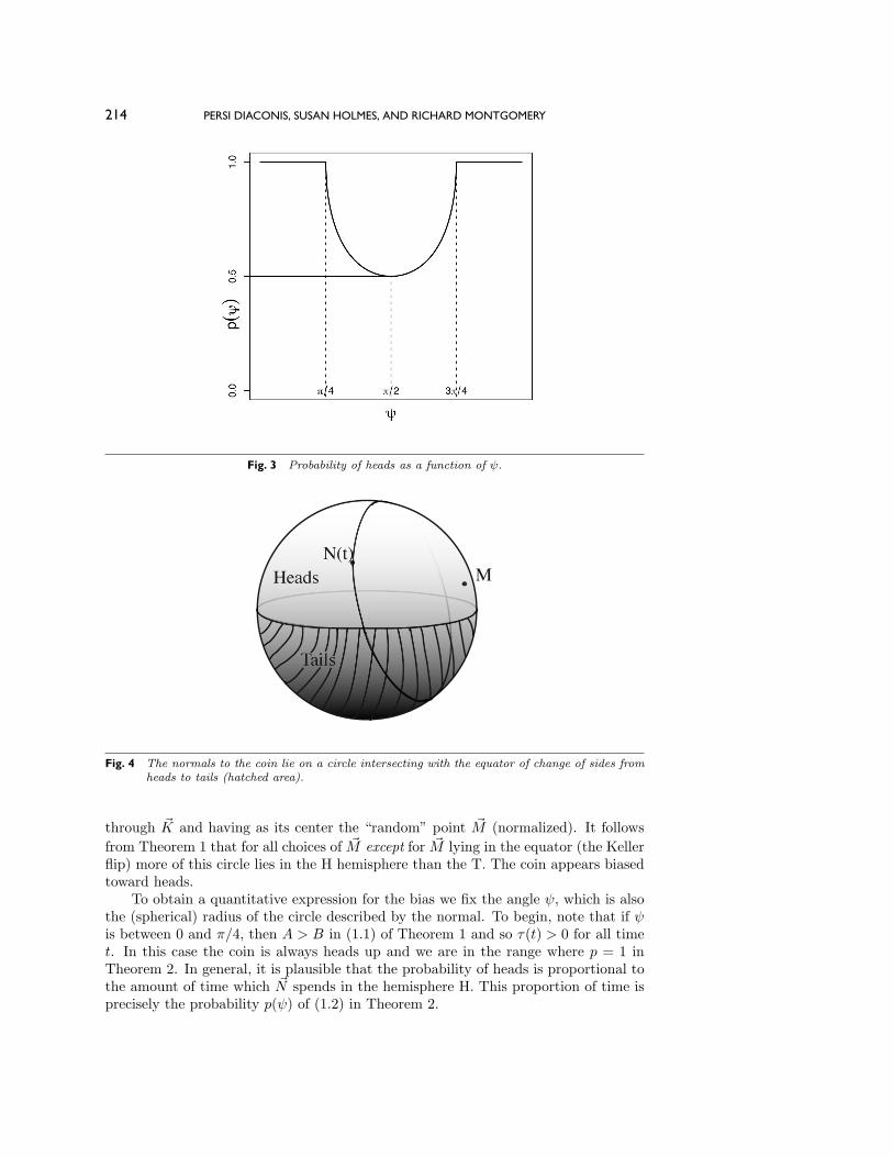
Theorem 2. For all smooth, compactly supported densities g, as the product ω0t0tends to infinity, the limiting probability of heads p(ψ) with ψ fixed, given that headsstarts up, is

(1.2) p(ψ) =

12 + 1

π sin−1(cot2(ψ)) if π

4 < ψ < 3π/4,1 if 0 < ψ < π/4 or 3π

4 < ψ < π.

A graph of p(ψ) appears in Figure 3. Observe that p(ψ) is always greater thanor equal to 1/2 and equals 1/2 only if ψ = π/2. In this sense, vigorously tossed coins((w0, t0) large) are biased to come up as they started, for essentially arbitrary initialdistributions g. The proof of Theorem 2 gives a quantitative rate of convergence top(ψ) as ω0 and t0 become large.

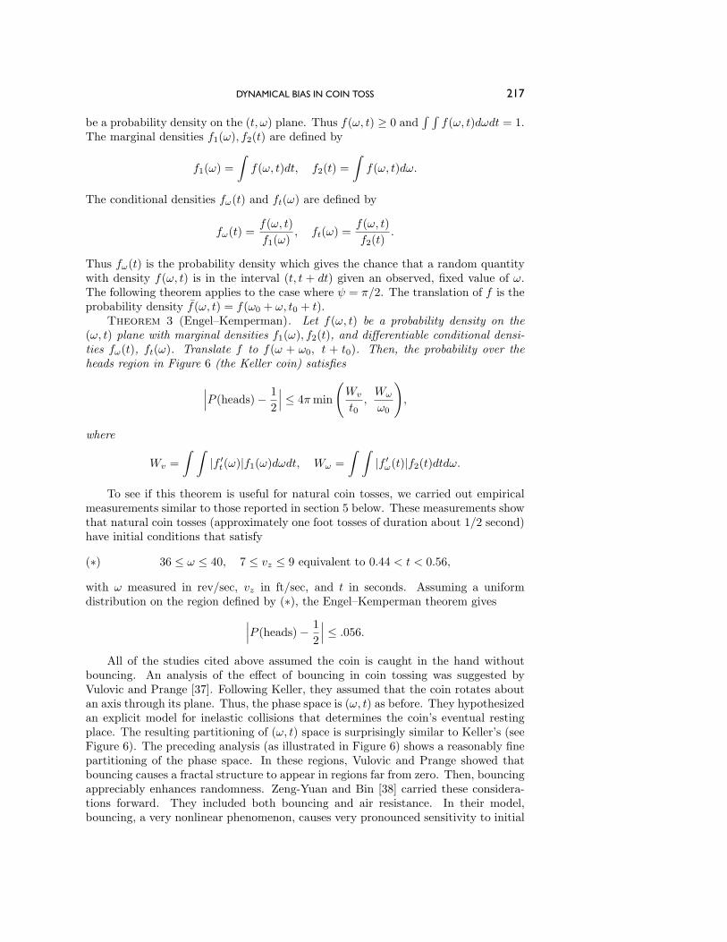
We now explain the picture behind Theorem 1 and some heuristics for Theorem2 (see Figure 4). While the coin is in flight its angular momentum is constant intime and the normal vector precesses around it at a uniform velocity, sweeping outa circle on the sphere of unit vectors. (This is proved in section 3.) On this sphere,draw the equator of vectors orthogonal to the direction K of “straight up.” Points onthe equator represent the coin when only its edge can be seen. Points in the upperhemisphere H represent the coin “heads up” and points in the lower hemisphere Trepresent the coin “tails up.” H corresponds to τ > 0 and T to τ < 0, where τ is thefunction of Theorem 1.

Suppose now that the coin starts its travel precisely heads up, so that the normalis aligned with K. Then the normal N traces out a circle on the sphere passing

214 PERSI DIACONIS, SUSAN HOLMES, AND RICHARD MONTGOMERY

Fig. 3 Probability of heads as a function of ψ.

Fig. 4 The normals to the coin lie on a circle intersecting with the equator of change of sides fromheads to tails (hatched area).

through K and having as its center the “random” point M (normalized). It followsfrom Theorem 1 that for all choices of M except for M lying in the equator (the Kellerflip) more of this circle lies in the H hemisphere than the T. The coin appears biasedtoward heads.

To obtain a quantitative expression for the bias we fix the angle ψ, which is alsothe (spherical) radius of the circle described by the normal. To begin, note that if ψis between 0 and π/4, then A > B in (1.1) of Theorem 1 and so τ(t) > 0 for all timet. In this case the coin is always heads up and we are in the range where p = 1 inTheorem 2. In general, it is plausible that the probability of heads is proportional tothe amount of time which N spends in the hemisphere H. This proportion of time isprecisely the probability p(ψ) of (1.2) in Theorem 2.

DYNAMICAL BIAS IN COIN TOSS 215

(a) (b)

Fig. 5 (a) Variations of the function τ as a function of time t for ψ = π/2. (b) Variations of thefunction τ as a function of time t for ψ = π/3.

Figures 5(a) and 5(b) show the effect of changing ψ. In Figure 5(a), ψ = π2 and

τ of (1.1) is positive half of the time. In Figure 5(b), ψ = π3 and τ is more often

positive.Theorems 1 and 2 lead us to ask what the empirical distribution of ψ is when

real people toss coins. In section 5 two empirical studies are described. The first islow-tech and uses a coin with a thin ribbon attached. The second uses a high-speedslow motion camera. The projection of a circle onto the plane of the camera is anellipse. Using image analysis techniques we fit the ellipses to the images of the tossedcoin. A simple function of the lengths of the major and minor axes gives the normalto the coin in three-space. As explained, these normals spin in a circle about theangular momentum vector which stays fixed during the coin’s flight. This gives anestimate of ψ. Two methods of estimation which agree to reasonable approximationare given.

The empirical estimates of ψ show that naturally flipped coins precess sufficientlyto force a bias of at least .01. We find it surprising that this bias persists in the limitof vigorously flipped coins for general densities g(ωN , t).

The structure of the rest of the paper is as follows. Section 2 reviews previousliterature and data on coin tossing. Section 3 reviews rigid body motion and provesTheorem 1. In section 3 we also derive an exact result for the amount of precession: theamount that the coin turns about its normal during one revolution of the normal aboutthe angular momentum vector is π cos(ψ). This “internal rotation” is an example of ageometric or Berry phase [29]. The limiting results of Theorem 2 are proved in section4. Section 5 presents our data. Section 6 presents some caveats to the analysis alongwith our conclusions.

2. Previous Literature. The analysis of classical randomization devices usingmechanics and a distribution on initial conditions goes back to Poincare’s analysis ofroulette [32, pp. 122–130]. This was brilliantly continued in a sequence of studies byHopf [15, 16, 17], who studied Buffon’s needle, introduced various mixing conditionsto prove independence of successive outcomes, and gave examples where the initialconditions still influence later states. Hopf began a classification of low order ordinary

216 PERSI DIACONIS, SUSAN HOLMES, AND RICHARD MONTGOMERY

Fig. 6 The hyperbolas separating heads from tails in part of phase space. Initial conditions leadingto heads are hatched, tails are left white, ω is measured in s−1.

differential equations by sensitivity to initial conditions. While this work is littleknown today, [36] gives some further history, [34] offers a philosopher’s commentary,and [5] presents a detailed development with extensions.

It cannot be emphasized too strongly that the results above are limiting results:Poincare’s arguments suggest that as a roulette ball is spun more and more vigorouslythe numbers become closer and closer to uniformly distributed. There are numerousstudies (see [1], [2]) suggesting that real roulette may not be vigorous enough to avoidthe perennity of the initial conditions.

The careful study of flipped coins was begun by Keller [20], whose analysis webriefly sketch here. He assumed that a coin flips about an axis in its plane with spinabout this axis at rate ω revolutions per second. If the initial velocity in the updirection K is vz, after t seconds a coin flipped from initial height z0 will be at heightz0 + tvz − (g/2)t2. Here g is the acceleration due to gravity (g .= 32 ft/(sec)2 if heightis measured in feet). If the coin is caught when it returns to z0, the elapsed time t∗

satisfies z0 + t∗vz − (g/2)(t∗)2 = z0 or t∗ = vz/(g/2). The coin will have revolvedωvz/(g/2) times. If, for some integer j, this number of revolutions is between 2j and2j + 1, the initial side will be upmost. If the number of revolutions is between 2j + 1and 2j+2, the opposite side will be upmost. Figure 6 shows the decomposition of thephase space (ω, t) into regions where the coin comes up as it started or opposite. Theedges of the regions are along the hyperbolas ωv/(g/2) = j. Visually, the regions getclose together so small changes in the initial conditions cause the difference betweenheads and tails.

The spaces between the hyperbolas in Figure 6 have equal area. The horizontalaxis goes from t = 0.1s to t = 0.8s. The vertical axis goes from ω = 0 to ω = 1400.

Asymptotic limits can be avoided by deriving explicit error terms for the approx-imations. Here is a theorem from [5], specialized to the coin tossing case. (Here weare still in Keller’s model, not in the context of Theorems 1 and 2 above.) Let f(ω, t)

DYNAMICAL BIAS IN COIN TOSS 217

be a probability density on the (t, ω) plane. Thus f(ω, t) ≥ 0 and∫ ∫

f(ω, t)dωdt = 1.The marginal densities f1(ω), f2(t) are defined by

f1(ω) =∫f(ω, t)dt, f2(t) =

∫f(ω, t)dω.

The conditional densities fω(t) and ft(ω) are defined by

fω(t) =f(ω, t)f1(ω)

, ft(ω) =f(ω, t)f2(t)

.

Thus fω(t) is the probability density which gives the chance that a random quantitywith density f(ω, t) is in the interval (t, t + dt) given an observed, fixed value of ω.The following theorem applies to the case where ψ = π/2. The translation of f is theprobability density f(ω, t) = f(ω0 + ω, t0 + t).

Theorem 3 (Engel–Kemperman). Let f(ω, t) be a probability density on the(ω, t) plane with marginal densities f1(ω), f2(t), and differentiable conditional densi-ties fω(t), ft(ω). Translate f to f(ω + ω0, t + t0). Then, the probability over theheads region in Figure 6 (the Keller coin) satisfies

∣∣∣P (heads)− 12

∣∣∣ ≤ 4πmin

(Wv

t0,Wω

ω0

),

where

Wv =∫ ∫

|f ′t(ω)|f1(ω)dωdt, Wω =∫ ∫

|f ′ω(t)|f2(t)dtdω.

To see if this theorem is useful for natural coin tosses, we carried out empiricalmeasurements similar to those reported in section 5 below. These measurements showthat natural coin tosses (approximately one foot tosses of duration about 1/2 second)have initial conditions that satisfy

(∗) 36 ≤ ω ≤ 40, 7 ≤ vz ≤ 9 equivalent to 0.44 < t < 0.56,

with ω measured in rev/sec, vz in ft/sec, and t in seconds. Assuming a uniformdistribution on the region defined by (∗), the Engel–Kemperman theorem gives∣∣∣P (heads)− 1

2

∣∣∣ ≤ .056.All of the studies cited above assumed the coin is caught in the hand without

bouncing. An analysis of the effect of bouncing in coin tossing was suggested byVulovic and Prange [37]. Following Keller, they assumed that the coin rotates aboutan axis through its plane. Thus, the phase space is (ω, t) as before. They hypothesizedan explicit model for inelastic collisions that determines the coin’s eventual restingplace. The resulting partitioning of (ω, t) space is surprisingly similar to Keller’s (seeFigure 6). The preceding analysis (as illustrated in Figure 6) shows a reasonably finepartitioning of the phase space. In these regions, Vulovic and Prange showed thatbouncing causes a fractal structure to appear in regions far from zero. Then, bouncingappreciably enhances randomness. Zeng-Yuan and Bin [38] carried these considera-tions forward. They included both bouncing and air resistance. In their model,bouncing, a very nonlinear phenomenon, causes very pronounced sensitivity to initial

218 PERSI DIACONIS, SUSAN HOLMES, AND RICHARD MONTGOMERY

(a) (b)

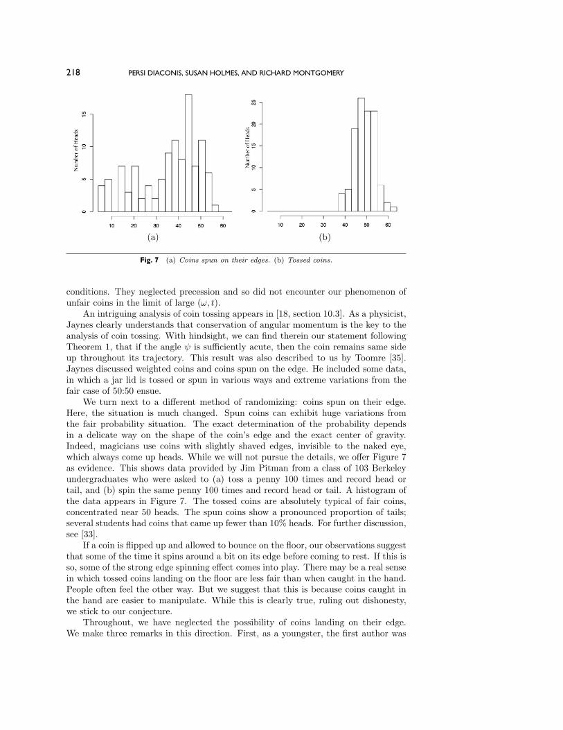
Fig. 7 (a) Coins spun on their edges. (b) Tossed coins.

conditions. They neglected precession and so did not encounter our phenomenon ofunfair coins in the limit of large (ω, t).

An intriguing analysis of coin tossing appears in [18, section 10.3]. As a physicist,Jaynes clearly understands that conservation of angular momentum is the key to theanalysis of coin tossing. With hindsight, we can find therein our statement followingTheorem 1, that if the angle ψ is sufficiently acute, then the coin remains same sideup throughout its trajectory. This result was also described to us by Toomre [35].Jaynes discussed weighted coins and coins spun on the edge. He included some data,in which a jar lid is tossed or spun in various ways and extreme variations from thefair case of 50:50 ensue.

We turn next to a different method of randomizing: coins spun on their edge.Here, the situation is much changed. Spun coins can exhibit huge variations fromthe fair probability situation. The exact determination of the probability dependsin a delicate way on the shape of the coin’s edge and the exact center of gravity.Indeed, magicians use coins with slightly shaved edges, invisible to the naked eye,which always come up heads. While we will not pursue the details, we offer Figure 7as evidence. This shows data provided by Jim Pitman from a class of 103 Berkeleyundergraduates who were asked to (a) toss a penny 100 times and record head ortail, and (b) spin the same penny 100 times and record head or tail. A histogram ofthe data appears in Figure 7. The tossed coins are absolutely typical of fair coins,concentrated near 50 heads. The spun coins show a pronounced proportion of tails;several students had coins that came up fewer than 10% heads. For further discussion,see [33].

If a coin is flipped up and allowed to bounce on the floor, our observations suggestthat some of the time it spins around a bit on its edge before coming to rest. If this isso, some of the strong edge spinning effect comes into play. There may be a real sensein which tossed coins landing on the floor are less fair than when caught in the hand.People often feel the other way. But we suggest that this is because coins caught inthe hand are easier to manipulate. While this is clearly true, ruling out dishonesty,we stick to our conjecture.

Throughout, we have neglected the possibility of coins landing on their edge.We make three remarks in this direction. First, as a youngster, the first author was

DYNAMICAL BIAS IN COIN TOSS 219

involved in settling a bet in which 10 coins were tossed in the air to land on the table(this to be repeated 1000 times). On one of the trials, one of the coins spun aboutand landed on its edge. An analysis of coins landing on edge has been developed byMurray and Teare [31]. Using a combination of theory and experiment they concludedthat a U.S. nickel will land on its edge about 1 in 6000 tosses. Finally, Mosteller [30]developed tools to study the related question, “How thick must a coin be to haveprobability 1/3 of landing on edge?”

In light of all the variations, it is natural to ask if inhomogeneity in the massdistribution of the coin can change the outcome. The papers [26] and [13] give informalarguments suggesting that inhomogeneity does not matter for flipped coins caught inthe hand. Jaynes reported that 100 flips of a jar lid showed no evidence of bias. Wehad coins made with lead on one side and balsa wood on the other. Again no biasshowed up. All of this changes drastically if inhomogeneous coins are spun on thetable (they tend to land heavy side up). As explained above, some of this bias persistsfor coins flipped onto a table or floor.

Coin tossing is such a familiar image that it seems that large amounts of empiricaldata should be available. A celebrated study [21] is based on a heroic collection of10,000 coin flips. Kerrich’s flips allowed the coin to bounce on the table so our analysisdoes not apply. His data do seem random (p = 1/2) for all practical purposes. Furtherstudies of Pearson (24,000 flips) and Lock (30,000 flips) are reported in [33].

Our estimate of the bias for flipped coins is p = .51. To estimate p near 1/2with standard error 1/1000 requires 1

2√n= 1/1000 or n .= 250, 000 trials. While not

beyond practical reach, especially if a national coin toss was arranged, this makes itless surprising that the present research has not been empirically tested.

3. Rigid Body Motion. This section sets up notation, reviews needed mechanics,and proves extensions of Theorems 1 and 2. Before plunging into details, it maybe useful to have the following geometric picture of a tumbling, flipping coin. Startthe coin heads up, its normal vector N aligned with the up direction K. The initialvelocities determine a fixed vector M (the angular momentum vector). Picture thisriding along with the coin, centered at the coin’s center of gravity, staying in a fixedorientation with respect to the coordinates of the room. The normal to the coin staysat a fixed angle ψ to M and rotates around M at a fixed rate ωN . At the same time,the coin spins in its plane about N at a fixed rate ωpr. This description is derived insection 3.1. Theorem 1 is proved in section 3.2 allowing the initial configuration of thecoin to be in a general position. The amount ∆A of precession during one revolutionof N about M is related to the angle ψ by ∆A = π cos(ψ). This is made precise intwo ways in section 3.3, where it is seen as a kind of “geometric Berry phase.” Asdescribed there, we found this a convenient way to empirically estimate the crucialangle ψ.

This section uses the notation and development of [25, Chapter 6]. A moreintroductory account of the mysteries of angular momentum appears in [9, Vol. I,Chapters 18–20]. The classical account of [14] spells out many details. An advancedtreatment appears in [28].

3.1. The Basic Setup. We model the flipping coin as a homogeneous, symmetricrigid body. Its center of gravity RG moves according to RG(t) = (X(0) + tVx, Y (0) +tVy, Z(0) + tVz − gt2/2), where V = (Vx, Vy, Vz)T is its initial velocity, and wherethe last coordinate is in the direction of gravity. In order to describe the tumblingof the coin we use two coordinate systems, both centered at RG. One has its axes

220 PERSI DIACONIS, SUSAN HOLMES, AND RICHARD MONTGOMERY

directions fixed relative to an inertial, or laboratory, frame. Coordinates and vectorsin this system are denoted by capital letters. The second coordinate system has itsaxes rigidly attached to the coin and is called the body frame, and its coordinatesand vectors are denoted by small letters. For example, the normal to the coin asviewed from the laboratory frame is N and depends on time, while the same normal,viewed in the body frame, is written n and is a constant vector along the z axis. Thetwo frames are related by a rotation matrix Γ(t), which takes a vector in the bodyframe to the same point in the laboratory frame. Thus, for example, Γ(0) = id andN(t) = Γ(t)n. For an introductory account of moving frames such as our body frame,see, for example, [10].

The instantaneous angular velocity Ω(t) is a way of encoding the time derivativeof Γ(t). It is a vector such that if X is pointing to a fixed material point on the coin,so that X(t) = Γ(t)x with x constant in the body frame, then

(3.1)d X

dt= Ω(t)× X.

It will be important to have a picture of the general solution X(t) to (3.1) in thecase where Ω(t) = Ω is constant. Then the projection of X(t) onto the line through Ωis constant, while the projection of X(t) onto the perpendicular plane to Ω traversesa circle at constant angular speed ‖Ω‖. Putting these two motions together, X(t)sweeps out a cone whose tip travels the circle centered at the projection of X(0) ontothe line through Ω, with the plane of this circle perpendicular to this line.

In general, Ω(t) changes with t. There are exactly two cases where Ω(t) is con-stant: the total cheat coin and the Keller coin, as discussed in section 1. Supposethat the coin starts heads up with the normal pointed up (in direction K). For the“total cheat coin,” Ω(t) is vertical, in line with the normal to the coin, and its lengthis constant. Then, the coin remains horizontal for all time and spins about the normaldirection with some constant angular speed ω (the length of Ω(t)). Equation (3.1)becomes

d X

dt= ω K × X.

For the “fair coin” analyzed by Keller, Ω(t) lies in the plane of the coin. If itsdirection is along I, then (3.1) becomes d X

dt = ωI × X, where again ω is the length ofthe (constant) vector Ω(t). This story was told in section 2. In all other cases, Ω(t)depends on t.

The evolution of the angular velocity can be determined by using the conservationof angular momentum and the linear relation between angular momentum and angularvelocity. While we will not need it explicitly, the angular momentum vector M for arigid body may be defined as a sum over particles a in the body,

(3.2) M =∑a

maRa × Va,

with Ra the distance of the ath particle from the center of gravity, Va its velocity, andma its mass. Conservation of angular momentum asserts that M is constant duringthe flight of the coin.

DYNAMICAL BIAS IN COIN TOSS 221

The vectors M and Ω(t) are related by a symmetric positive definite matrix calledthe moment of inertia tensor [25, section 32]. This matrix is constant relative to thebody frame. Its eigenvalues are called the principal moments of inertia and denotedI1, I2, I3. Because of the coin’s symmetry, I1 = I2 and the eigenvectors for I1, I2 spanthe plane of the coin. Let e1, e2 be a basis of this plane. The eigenvector for I3 isn, the normal to the coin. If the coin is modeled as a solid cylinder of thickness h,radius ρ, and uniform density, then [25, p. 102, eq. 2(c)] shows that

(3.3) I1 = I2 =14

(mρ2 +

13mh2

)and I3 =

12mρ2,

where m is the total mass. Note that in the h ↓ 0 limit (i.e., a very thin coin)I1 ∼ I3/2. The experiments described in section 5 use a U.S. half dollar, which has

h = 2.15mm, ρ = 15.3mm, m = 11.34g.

Thus I1 = I2 = 0.681g.m2 and I3 = 1.327g.m2.

Let ω, m be the angular velocity and angular momentum in the body frame. Thusω = Γ(t)−1Ω and m = Γ(t)−1 M . Expanding them out in terms of the eigenframee1, e2, n yields

ω = ω1e1 + ω2e2 + ω3n,

m = m1e1 +m2e2 +m3n.

The components ωi and mi will depend on t in general. Applying the moment ofinertia tensor to ω yields m, where

(3.4)m = I1ω1e1 + I2ω2e2 + I3ω3n

= I1ω + (I3 − I1)ω3n,

where we have used that I1 = I2. We now apply the rotation matrix Γ(t) relating thetwo frames to obtain

M = I1Ω+ (I3 − I1)ω3 N.

Solving for Ω gives

(3.5)Ω =

1I1M +

(1− I3

I1

)ω3 N

= ωNM − ωpr N,

where

(3.6) ωN =M/I1, ωpr =

(1I1− 1I3

)M cos(ψ), M = M/M,

M = ‖ M‖ is the magnitude of the angular momentum M , and we have used M3 =M cos(ψ) = I3ω3. We note that ωpr is positive since I1 < I3.

The vectors M and Ω(t) are parallel precisely at the extremes of the total cheatcoin and the fair coin. In the total cheat case the components ω1 = ω2 = 0, the

222 PERSI DIACONIS, SUSAN HOLMES, AND RICHARD MONTGOMERY

vectors M and N are proportional and constant in time, and M = I3Ω, so that Ω isalso constant in time. In the fair case, the component ω3 is zero, M = I1Ω, and againΩ is constant in time. In all other cases, the angular momentum and velocity vectorsare not parallel. The vector M stays constant in laboratory coordinates, while N andΩ move in laboratory coordinates.

From (3.1) and (3.4)–(3.6) we can read off the geometric description which intro-duced this section. Equation (3.1) applies to the vector X = N since n is fixed in thecoin frame. Thus

d N

dt= Ω(t)× N.

Then, (3.5) along with N × N = 0 imply

(3.7)d N

dt= ωNM × N.

This equation asserts that the coin’s normal vector precesses about the axis M andthat the angular frequency of precession is ωN = M/I1, as in (3.6). The followingsection solves (3.7) and uses this to prove Theorem 1.

3.2. A Generalization of Theorem 1. In the inertial frame K is a unit vectorin the up direction, M is the unit vector in the direction of the angular momentum,and N(t) is the unit normal to the head of the coin. The coin is “up” if K · N > 0and “down” (tails) if K · N < 0. Theorem 1 assumes that the coin starts with headsperfectly up ( K = N at time 0). The following extensions allow an arbitrary start forN .Theorem 1

∗. Let f(t) = N(t) · K be the quantity which determines “heads” or

“tails,” i.e., the cosine of the angle between the normal N(t) to the coin at time t andthe up direction K. Define ψ, φ by

cos(ψ) = N(0) · M,cos(φ) = K · M ;

then

f(t) = A+B cos(ωN t+ θ0),

with A = cosψ cosφ,B = sinψ sinφ, ωN =M/I1 for I1 given by (3.3), and the phaseθ0 is determined by K · N(0).

Note that if N(0) = K so the coin starts heads “exactly” up, then ψ = φ andTheorem 1∗ yields Theorem 1. (We will see in the proof—look at the definition of G1there—that in this case θ0 = 0 also.)

We have presented Figure 8 in order to help interpret Theorem 1∗ and Theorem2∗. Figure 8 represents a sphere of possible unit vectors M , with the two points N(0)and K indicated along with their corresponding great circles (“polars”), which are theloci of points where N(0) · M = 0 and where K · M = 0. The shaded region betweenthese great circles is the region where M must be located in order for the coefficientA to be negative, and consequently in this region (see Theorem 2∗) the asymptoticbias is toward tails as opposed to heads.

DYNAMICAL BIAS IN COIN TOSS 223

Fig. 8 The situation of Theorem 1∗. N(0) and the vertical K need not be equal. When M is in theshaded region the asymptotic bias is toward tails.

Proof. From (3.7) for any t ≥ 0, cosψ = N(0) · M = N(t) · M : the normal to thecoin makes a constant angle with the angular momentum vector. Introduce a neworthonormal basis for space (G1, G2, M), with G1 in the plane spanned by M and K,so that G2 is perpendicular to both M and K. Then, from the definition of φ,

K = sin(φ)G1 + cos(φ)M.

The general solution of the first order linear differential equation (3.7) for N(t) isN(t) = aM + b(G1cos(ωN t + θ0) + G2 sin(ωN t + θ0). The initial value of N(0) · Mdetermines a = cos(ψ), b = sin(ψ). (The value of θ0 can be determined from N(0) · Kif needed.) Altogether,

N(t) = cos(ψ)M + sin(ψ)cos(ωN t+ θ0)G1 + sin(ωN t+ θ0)G2.

The expression for f(t) = N(t)·K follows from the orthonormality of (G1, G2, M).This completes the proof of Theorem 1 as well.The analytic argument of section 4 shows that for vigorously flipped coins the

argument ωN t of f in Theorem 1∗ is asymptotically uniformly distributed (mod 2π).The following theorem extends Theorem 2 to the case where the coin does not startwith heads perfectly up. The setup is exactly the same as that preceding Theorem 1∗.In addition, we let ω and t tend to infinity in the following way. For all a, b nonzero,we start with a compactly supported probability density g(ω, t)dωdt, and translateit along a ray ω/t = a/b by forming gλ(ω, t)dωdt = g(ω − λa, t − λb)dωdt. Here aand b are fixed parameters which define the direction of the ray and λ parameterizesthe distance along the ray. Then we compute the probability p(ψ, φ;λ) of heads withrespect to gλ, given that we started with the angular momentum making an angleψ to the normal and an angle φ to the up direction. Then we take the limit of thisprobability as λ→ +∞. Theorem 5 shows that this limit exists; we will call it p(ψ, φ).

Theorem 2∗. Let ψ, φ, 0 ≤ ψ, φ ≤ π/2, be defined as in Theorem 1∗. As ω and ttend to infinity, let p(ψ, φ) be the limiting probability of heads for a coin toss, startingwith heads up, with angle ψ between the normal

N(0) to the coin and the angular

momentumM , and angle φ between the up direction

K and

M . Then

p(ψ, φ) =

12 + 1

π sin−1(cot(φ) cot(ψ)) if (cotφ)(cotψ) ≤ 1,1 if (cot(φ)) cot(ψ) ≥ 1.

224 PERSI DIACONIS, SUSAN HOLMES, AND RICHARD MONTGOMERY

Proof. According to Theorem 5 of the next section, the limiting probabilitydistribution of the angle θ = ωN t is uniformly distributed on [0, 2π). We must thenevaluate the probability that f(θ) > 0, where θ is uniformly distributed and f isthe function of Theorem 1∗. We have f(θ) = A + B cos(θ) with A = cos(ψ) cos(φ),B = sin(ψ) sin(φ). If A > B, then f(θ) > 0 for all θ and p = 1. This happens if andonly if cot(φ) ·cot(ψ) > 1. To compute in the case A ≤ B observe that f is symmetricabout θ = π and is monotone decreasing on (0, π). It follows that f has a unique zeroθ1 in (0, π), that f is positive on 0 < θ < θ1, and that f is negative on θ1 < θ ≤ π.The uniform measure of the set θ : f(θ) > 0 is then

p(ψ, φ) = θ1/π.

The zero θ1 occurs when cos(θ) = −A/B. So θ1 = cos−1(−A/B). Using cos(π2 +h

)=

− sin(h) gives θ1 = π2 + sin−1(A/B). Finally, A/B = cotφ cotψ.

This completes the proof of Theorem 2 as well.

3.3. Precession of the Head. As explained in the introduction to this section,while the normal to the coin is spinning about the angular momentum vector at rateωN , the coin is also spinning about the normal at a constant rate ωpr. We now furtherquantify and verify that assertion.

Theorem 4. With notation as in (3.3), (3.6), each time the normal vectorcompletes one full cycle around the angular momentum vector, the coin has precessedby the angle

∆A = −ωprωN

2π = −(1− I1/I3)2πcos(ψ)(3.8a)

∼ −πcos(ψ) as h ↓ 0.(3.8b)

Remark. When ψ 0 so that M is nearly aligned with the vertical, we have∆A π. In other words, every time the normal vector precesses around once, thecoin rotates approximately 180. Feynman observed this phenomenon in a Cornelldining hall. In his own words,

“some guy, fooling around, throws a plate in the air”. By noticing thedifference between the plate’s angular velocity and that of the associatedwobble, says Feynman, he was motivated to higher things: “The diagramsand the whole business that I got the Nobel Prize for came from thatpiddling around with the wobbling plate.” [8]

Remark. While the angular momentum and ψ are difficult to measure directly,the slow motion photography explained in section 5 often produced two frames wherethe coin clearly completed one revolution and the angle ∆A could be measured. From(3.8b), this gives ψ. An example is shown in Figure 9. A second method of estimatingψ from photographs is explained in section 5.2 below. In this second method onereconstructs the normal’s time evolution and uses this to determine the radius (againψ) of the resulting circle on the sphere. We have used four photographed tosses tocheck the first method. For toss no. 27, this method produced an estimate ψ of ψ.We observed ψ = 1.48. For toss no. 30 we get ψ = 1.47; for toss no. 32, ψ = 1.40;and for toss no. 33, ψ = 1.36. These are in close agreement with the first method ofestimation.

Proof. Our proof relies on Euler’s description of the motion of a rigid body,essentially the dual to (3.1) [25, sections 36, 36.5–36.7]. Let X be a vector which isfixed in space, and let x be the corresponding vector, viewed in the body frame. Then

DYNAMICAL BIAS IN COIN TOSS 225

Fig. 9 Theorem 4 illustrated; these images are separated by exactly one coin flip.

Euler asserted that dx/dt = −ω(t)× x. Euler’s equation is obtained by taking for Xthe angular momentum M ,

dm/dt = −ω(t)× m.

Since ω = ωN m− ωprn (see (3.5)) and since m× m = 0 Euler’s equation becomes

(3.9) dm/dt = ωprn× m.

To complete the proof, we have N(T ) = N(0), where T = 2π/ωN is the period of N ’sprecession. The evolution equation (3.9) for m asserts that the projection b of m ontothe plane of the coin precesses at frequency ωpr relative to a frame rigidly attachedto the coin. (See the geometric description following (3.1).) Consequently, after timeT the vector b has rotated by an amount ωprT . In the meantime, in the lab framethe plane of the coin has returned to its original position and the vector M has notmoved. But b is simply the projection of M , viewed relative to the coin’s frame. Itfollows that the coin’s frame has rotated by −ωprT = ∆A about the normal in thesame time.

4. Uniformity of Angular Distribution. The proof of Theorems 2 and 2∗ relieson the assertion that θ = ωN t, modulo 2π, tends to the uniform distribution on theinterval [0, 2π). It remains to establish this uniformity. The key is a theorem statingthat if we take any “nice” real random variable X, rescale it, and view the resultmodulo 2π, then as the rescaling tends to infinity, the distribution of the randomvariable becomes uniform. In symbols, λX mod 2π tends to the uniform distributionU on the interval [0, 2π) as λ → ∞. Such scaling theorems were used in Poincare’soriginal treatment of roulette. A comprehensive treatment is in [5]. The main theoremof this section, Theorem 5 below, establishes a quantitative version of the neededuniformity.

The product ωN t(mod 2π) depends on the initial conditions:

ωN = ‖ M‖/I1 and t = tc = vz/(g/2).

(See (3.3) and (3.6).) For vigorously flipped coins ‖ M‖ and vz will be large. Toformalize this “largeness” we suppose that the joint probability distribution of ω = ωNand t is of the form g(ω−ω0, t− t0), where the product ω0t0 is large and where g(ω, t)

226 PERSI DIACONIS, SUSAN HOLMES, AND RICHARD MONTGOMERY

is a smooth probability density (C1 is enough) with compact support. Note that ω0t0is unitless and corresponds to the number of flips. Further, the expectation of ω is oforder ω0, and that of t is of order t0.

The argument we are about to present is a variant of one due to Engel and Kem-perman and developed in Chapters 2 and 3 of [5], which we strongly recommend. Forease of notation and proof we abstract. Let (Xλ, Yλ) be a family of real-valued ran-dom variables parameterized by the ray 0 < λ < ∞. The following two assumptionsare needed:

For some c > 0 there is a γ > 0 so that for all λ,

P (Yλ < λc) ≤ γ/λ.(4.1)

For each λ and each fixed y, there is a regular conditional

probability distribution for Xλ given Yλ = y, withdifferentiable density pXλ(x|Yλ = y), satisfying∫

|p′Xλ(x|Yλ = y)|pYλ(dy) = Aλ <∞.

(4.2)

Assumption (4.1) is a way of saying that Yλ →∞ with λ. Assumption (4.2) is a way ofsaying that the marginal density of Xλ at x, which is

∫pXλ(x|Yλ = y)pYλ(dy), is not

too sharply peaked for any x. In our application λ parameterizes a ray in the positive(ω, t) orthant, and Xλ = ωN and Yλ = tc are assumed to be distributed according tog(ω−λω0, t−λt0). For g smooth with compact support, both assumptions (4.1) and(4.2) are satisfied with Aλ uniformly bounded.

The statement of the next theorem involves the variation distance between twomeasures µ, v. This distance is defined by

dv(µ, v) = supC|µ(C)− v(C)|

=12

∫ ∣∣∣dµdσ− dvdσ

∣∣∣dσ,with the sup over all measurable sets C. In the second equality σ is any measure whichdominates both µ and v (for example, σ = µ + v). Note that this second equalityis independent of σ. If X and Y are random variables with µ(C) = P (X ∈ C),ν(C) = P (Y ∈ C) we write dv(X,Y ) for dv(µ, ν). A careful treatment of variationdistance is in [5].

Theorem 5. Let (Xλ, Yλ) be a family of real-valued random variables satisfying(4.1), (4.2). Let U be a uniform random variable taking values on the interval [0, 2π].Then, for all λ,

dv(XλYλ(mod 2π), U) ≤ γλ+π

4cAλλ.

Proof.

dv((XλYλmod 2π), U) ≤∫dv(Xλy(mod 2π), U)Pyλ(dy)

≤ PYλ ≤ cλ+∫Yλ≥cλ

dv(Xλy(mod 2π), U)PYλ(dy)

≤ γλ+∫Yλ≥cλ

π

4y

∫|p′Xλ(x|Yλ = y)|dxPYλ(dy)

≤ γλ+π

4cλAλ.

DYNAMICAL BIAS IN COIN TOSS 227

The first inequality follows from Proposition 2.8a of [5]. This says that if X and Yare real-valued random variables and Z is a random variable defined on the sameprobability space, then

dv(X,Y ) ≤∫dv(Xz, Y )Pz(dz),

withXz the random variable conditional on Z = z. The second inequality uses dv ≤ 1.The third inequality uses (4.1) and Theorem 3.3 of [5], the theorem mentioned in thefirst paragraph of the present section. This theorem states that for a real randomvariable X with differentiable density p(x),

dv(tX(mod 2π), U) ≤ π

4t

∫|p′(x)|dx.

The last inequality uses assumption (4.2).Remarks.(1) The roles of Xλ, Yλ can be reversed and the minimum of the two resulting

bounds used.(2) The rate of convergence, order 1/λ, is the best possible. However, there are

classes of examples where the convergence in Theorem 5 is exponential in λor even faster. See [5, Chapter 3] for the full range of possibilities.

(3) In the present application the convergence of XλYλ(mod 2π) to U is usedin conjunction with f(θ) of Theorem 1∗ to obtain Theorem 2. Since f is abounded continuous function, weak-star convergence to U will do. [5] showsthat λX(mod 2π) converges weakly to U if and only if the Fourier coefficientsofX(mod 2π) converge to zero. Thus densities such as g(ω, t) are not requiredfor Theorem 2 to hold.

5. Estimating Angular Momentum. The empirical distribution of the angle ψbetween the angular momentum vector M and the normal to the coin figures cruciallyin our analysis of coin tossing. In this section we describe our efforts at estimatingthis distribution for real flips of a U.S. half dollar.

We carried out two types of experiments. Our “low-tech” experiment involvedflipping a coin with a ribbon attached. After the flip the ribbon is unwound, showinghow many times the coin rotated. This is described in section 5.1. Our “high-tech”experiment involved a high-speed camera and the mathematics of section 3 to estimatethe sequence of normals to the coin at different times during the coin’s flight. Theselie on a circle centered at the angular momentum vector. The radius of this circlegives an estimate of ψ. These results are described in section 5.2. This estimate ofψ can be calibrated with the measured value of rotation of the coin’s face using therelation between this angle and ψ described in (3.8).

5.1. Coin and Ribbon. A 1/8-inch wide 29-inch long ribbon was attached to aU.S. half dollar with Scotch tape. For each flip, the ribbon was flattened (untwisted),with the end held in the left hand. The coin was positioned heads up, in a fixedorientation in a fixed coordinate system marked on a table. The coin was given anormal flip with the right hand, caught without bouncing at approximately the sameheight. For all flips that resulted in heads up, two numbers were recorded:

• The angle θ that a fixed point on the coin’s head made with its originalstarting orientation. Here −180 < θ < 180 with 180 and −180 indistin-guishable. The angle was measured to the nearest 5.

228 PERSI DIACONIS, SUSAN HOLMES, AND RICHARD MONTGOMERY

Fig. 10 Scatterplot of ribbon data.

• The number f of complete flips of the coin, determined by unwinding theribbon until it was untwisted.

Pairs (θ, f) were recorded for 100 flips (1 ≤ i ≤ 100). A scatterplot of these valuesappears in Figure 10. There are three noticeable features:

1. Four of 100 flips have f = 0 (the coin never turned). These were vigorousflips with θ ranging widely. This indicates that the angular momentum vectormakes angle at most 45 with the normal with probability roughly 1/25. Re-enforcing this, 3 of 100 flips have f ≡ 1.

2. The angles θ vary widely. They have minimum of−170, lower quartile −1.3;median and mean about 30, upper quartile of 55; and maximum of 180. Ifthe angular momentum vector was in the plane of the coin (ψ = π/2), thenall of these θi would be zero.

3. The (θ, f) pairs seem independent of each other (corr = −.2). Indeed, thedistribution of θ seems roughly uniform. One explanation is that the markedpoint on the coin makes several turns around.

All three observations reinforce the idea that typical coin flips often have the angle ψfar from π/2.

5.2. Slow Motion Photography. We used a high-speed slow motion camera torecord 50 coin flips. The camera, developed by Stanford’s digital photo program,shoots at up to 1400 frames per second (see [6], [23]). We found it best to filmat about 600 frames per second. In contrast, the slow motion feature on standardcamcorders shoots at about 60 frames per second which is much too slow to give anyuseful data.

The data collection and processing led to interesting, difficult problems. Briefly,our camera gave about 100 frames per flip. At 600 frames per second, this gives awindow of 1/6 seconds to record. We found careful effort is required to start thefilming so that enough of the flip was recorded.

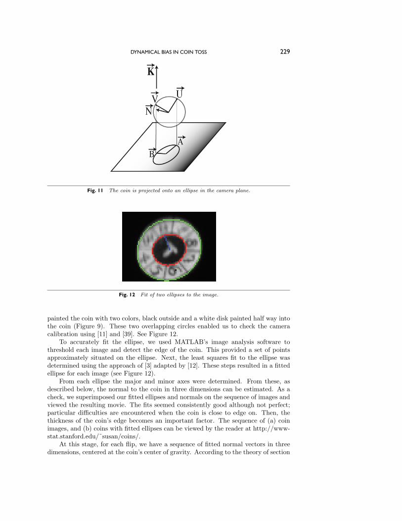
A successful filming results in up to 100 two-dimensional images. As explainedbelow, a circular disc projected onto a plane results in an ellipse (see Figure 11). We

DYNAMICAL BIAS IN COIN TOSS 229

Fig. 11 The coin is projected onto an ellipse in the camera plane.

Fig. 12 Fit of two ellipses to the image.

painted the coin with two colors, black outside and a white disk painted half way intothe coin (Figure 9). These two overlapping circles enabled us to check the cameracalibration using [11] and [39]. See Figure 12.

To accurately fit the ellipse, we used MATLAB’s image analysis software tothreshold each image and detect the edge of the coin. This provided a set of pointsapproximately situated on the ellipse. Next, the least squares fit to the ellipse wasdetermined using the approach of [3] adapted by [12]. These steps resulted in a fittedellipse for each image (see Figure 12).

From each ellipse the major and minor axes were determined. From these, asdescribed below, the normal to the coin in three dimensions can be estimated. As acheck, we superimposed our fitted ellipses and normals on the sequence of images andviewed the resulting movie. The fits seemed consistently good although not perfect;particular difficulties are encountered when the coin is close to edge on. Then, thethickness of the coin’s edge becomes an important factor. The sequence of (a) coinimages, and (b) coins with fitted ellipses can be viewed by the reader at http://www-stat.stanford.edu/˜susan/coins/.

At this stage, for each flip, we have a sequence of fitted normal vectors in threedimensions, centered at the coin’s center of gravity. According to the theory of section

230 PERSI DIACONIS, SUSAN HOLMES, AND RICHARD MONTGOMERY

3, these normals lie on a circle centered at the fixed angular momentum vector. Theradius of this circle thus gives an estimate of the angle ψ associated with the flip. Ofcourse, the circles can be fit from just a few points. We used about 20 points/flip andagain checked visually to see if these looked as if they lay on a circle. Some surprisingresults are described following the basic normal fitting algorithm which is describednext.

The plane of the camera is fixed throughout. In spatial coordinates (X1, X2, X3),the (X1, X2, 0) plane will be identified with the camera plane and the line (0, 0, X3) isthe orthogonal to the camera plane. At a fixed time, the coin is in a fixed position inthree-space. The projection of a circle or disc onto a plane is an ellipse. We observe,and can accurately estimate, the major and minor axes of this ellipse. The assumptionof orthographic projection implies that the length of the major axis is the same as thelength of the diameter of the coin. Without loss of generality we assume the coin hasradius 1. Let A = (A1, A2, 0) be a unit vector in the plane of the camera centered atthe ellipse, center along the major axis. Let B = (B1, B2, 0) be an orthogonal vectoralong the minor axis. Thus | A| = 1 and | B| = cos θ for some angle θ, 0 ≤ θ ≤ π/2.This description of A, B involves a choice of ± sign which we will deal with in amoment.

Throughout, we assume that coordinates have been chosen so that the center ofthe coin is at the center of the ellipse.

Let U, V be the unit vectors on the coin, which project to A, B, respectively, sothat in fact A = U . Let K = (0, 0, 1) be the direction orthogonal to the camera plane.

Lemma 1. With notation as above the normal N to the coin is

N =(ε1A2

√1− (B2

1 +B22), ε2A1

√1− (B2

1 +B22), ε3(A1B2 −A2B1)

)for some choice of signs εi = ±1.

Proof. Any vector projecting onto B has the form V = B + λ K. Since our Vis a unit vector and | B| = cos(θ), |λ| = sin θ is forced. Thus N = A × V = A ×( B+ ε sin θ K). Expanding out the cross product and using sin θ = ±

√1− (B2

1 +B22)

yields the result.Remark. The sign ambiguity creates a serious practical problem. If the coin

is parallel to the plane of the camera or edge onto the camera, the sign is difficultto determine (the projections in these cases are either perfect circles or a segment).While these events happen rarely with a tumbling coin, they do occur periodicallyand an arbitrary choice leads to physically ridiculous pictures. We resolved the choiceof signs by continuity, choosing (at each time frame) among eight sign patterns thatmakes the inner product of the current normal and previous normal as close as possibleto a constant, while keeping the curvature of the curve of normals continuous.

Figure 13(b) shows the result of this unscrambling process. In Figure 13(a) wesee the sequence of three-dimensional normals as they come from the computation ofnormals one by one from the ellipses. Successive normals are numbered in sequence.There are some approximately circular arcs; however, the result is a mess. In Fig-ure 13(b) we see that the unscrambled normals, unscrambled by appropriate choiceof signs, all lie clearly around the circle. Our theory implies that these points lie in aplane in three-dimensional space. We fit the plane using least squares. We computethe distance d between the plane and the origin from which we can find ψ = cos−1(d).

5.3. The Results. Of our 50 flips, 27 gave useful final results. From the measuredvalues of ψ, the probability p(ψ) was calculated from Theorem 2. The estimated prob-

DYNAMICAL BIAS IN COIN TOSS 231

(a)

(b)

Fig. 13 (a) The normals originally have a scrambled sign pattern. (b) How the normal vectors(once unscrambled) sit around a circle in three dimensions.

abilities range from 0.500 to 0.545. The 27 probabilities are displayed in a stem andleaf plot in Table 1. The first row of this plot shows the values 0.500, 0.500, 0.501, . . .indicating occurrences of flips for which p(ψ) took on these values. The next-to-lastrow shows no occurrences between 0.540 and 0.545. The last row shows the singleoutlying value 0.545. The median and standard deviation are 0.5027 and 0.0125. Themean of these probabilities is 0.508, and we have rounded this up to the 0.51 quoted.

232 PERSI DIACONIS, SUSAN HOLMES, AND RICHARD MONTGOMERY

Table 1 Stem and leaf plot of the estimated probabilities.

50 00111111122233333450 55551 35152 352 953 34535454 5

Table 2 Estimates of ψ of Theorem 2.

1.3697 1.2125 1.4682 1.2778 1.31031.2611 1.5528 1.4478 1.5211 1.51821.5100 1.2560 1.4797 1.4829 1.47051.5228 1.4696 1.5114 1.5102 1.49831.4962 1.4603 1.5176 1.4408 1.45191.5489 1.4800

For completeness, Table 2 shows the ψ values; these have mean 1.446 and standarddeviation 0.097. Note that if x denotes the mean of x, then p(ψ) = p(ψ).

6. Some Caveats to the Analysis. In carrying out the present analysis we makea number of assumptions. In this section we point out naturally occurring situationswhere our assumptions are violated, and hence our analysis need not apply.

6.1. Random In, Random Out. We have assumed that the coin is flipped witha known side uppermost. In many occurrences of coin tossing a coin is removed fromthe pocket and hence may be assumed as equally likely to start heads up as tails up.The physics preserves this: the outcome is as equally likely to end heads up as tailsup. We have friends who preface a coin toss by vigorously shaking the coin betweentheir cupped hands.

6.2. No Air Resistance. Throughout, we have neglected the effect of air resis-tance. Let us begin by acknowledging that air resistance is a potential confoundingfactor. Some friends in the physics department convinced us of this by dropping aU.S. penny off Stanford’s Hoover Tower. Some of the time it fell like a leaf, flutter-ing to the ground. We believe that for our short flips, air resistance has a negligibleeffect. One way to test this is to observe the time t1 that a coin takes to go fromits start to the top of its trajectory and then the time t2 that the coin takes to fallback to its initial starting height. As discussed in [4] air friction forces t2 > t1. Weexpect the size of this effect to be very small and an accurate measurement of it tobe very difficult. Zeng-Yuan and Bin [38] included air resistance in their analysis ofcoin tossing, presuming the effect is proportional to velocity. In the limit t → ∞ ofTheorems 2 and 2∗ air resistance could be nonnegligible.

Careful modeling of a spinning coin in a retarding medium seems like a difficultproblem. Even determining an appropriate approximation to the effect of friction onvelocity is a contentious matter. Long and Weiss [27] discussed the classical assump-tion (frictional force proportional to velocity) in detail and argued that velocity raisedto powers such as 3/2 or 2 seems more appropriate.

DYNAMICAL BIAS IN COIN TOSS 233

We do not believe that air resistance is a problem for naturally flipped coins, butas a referee pointed out, it probably is a problem in the large spin, large time of flightlimit. This is one of the reasons we gave quantitative nonlimiting results in section 4.

6.3. Definition of Time in Flight. We have used two different notions of thetime tc that the coin comes to rest (sections 3.1, 5.2). We have not incorporated thevery real possibility that the time tc has extra randomness due to the catcher’s handmoving, or a psychological component due to the coin being caught early or late in itsflight. We do not think that these variations in tc materially affect our conclusions.The reason is that flipped coins (starting from heads up) simply spend more of theirtotal time in flight heads up. Figure 4 shows this clearly. If the coin were caughtat a completely random time (say, uniformly chosen in a large interval), our analysiswould still apply.

6.4. Start Heads Up?. Perhaps the most vulnerable assumption is the specifi-cation of the starting normal direction as heads exactly up. Careful observation ofnatural flips shows some play in the initial position due to the position of the hand andthumb. We have dealt with this mathematically in section 3.2 but have not gathereddata. Of course, this point is closely connected to point 6.1 above.

6.5. No Bouncing. We have assumed that the coin is caught without bouncing.While this is a very common occurrence, we note that often a flipped coin is caughtin the hand and then slapped down on the table or on the back of the other hand,turning it over once. Of course, this last results in a bias opposite to the start. If themethod of catching is not determined (sometimes flipped over, sometimes as fallen),a significant amount of randomness may be added.

Often, flipped coins are allowed to land on hard surfaces and bouncing occurs.This requires a different type of analysis. Some further discussion and references arein section 2.

6.6. The Pragmatic Uncertainty Principle. The measurements recorded in sec-tion 5 may have affected the outcomes recorded. For example, attaching a ribbonto the coin changes the aerodynamics of its flight. To check this, we recorded theangle θ for 100 flips of a half dollar without the ribbon attached. The results werestill widely spread out but now the lower, median, and upper quantiles were shiftedto −40, 0, 30. Similarly, getting the slow motion camera in sync with our flipsrequired fairly artful flips. These seem quite different from the more vigorous flipsone observes at sporting events. We hope to develop a setup with multiple low-speedcameras that allow measurement of more natural flips.

7. Conclusion. Despite these important caveats we consider the bias we havefound fascinating. The discussion also highlights the true difficulty of carefully study-ing random phenomena. If we have this much trouble analyzing a common cointoss, the reader can imagine the difficulty we have with interpreting typical stochasticassumptions in an econometric analysis.

The caveats and analysis also point to the following conclusion: Keller’s analysisgives a good approximation for tossed coins. To detect the departures of the order ofmagnitude we have found would require 250,000 tosses. The classical assumptions ofindependence with probability 1/2 are pretty solid.

Acknowledgments. Thanks to Ali Ercan and Abbas El Gamal for providingthe camera images. Aharon Kapitulnik and Steve Shenker provided valuable ad-vice about air resistance. Summer undergraduate student Varick Erickson, funded

234 PERSI DIACONIS, SUSAN HOLMES, AND RICHARD MONTGOMERY

through a Stanford VPUE grant, refined the thresholding and edge detection proce-dures. Thanks to Vincent Fremont for his two-circle calibration code, Jim Pitmanfor the Berkeley toss and spin data, and M. Franklin for letting her technicians buildthe coin flipping machine. We also thank Roy Goodman and his students from NJITfor their feedback, Joe Keller for numerous conversations over the years, and JimIsenberg for an invitation to talk on an early version of this paper at the Universityof Oregon. Finally, we thank the editors and six referees for their detailed comments.

REFERENCES

[1] R. Barnhart, Beating the Wheel: Winning Strategies at Roulette, Lyle and Stuart, New York,1992.

[2] T. Bass, The Eudaemonic Pie, Houghton-Mifflin, Boston, 1985.[3] F. L. Bookstein, Fitting conic sections to scattered data, Comput. Graphics Image Process,

9 (1979), pp. 56–71.[4] F. Brauer, What Goes Up Must Come Down, Eventually, Amer. Math. Monthly, 108 (2001),

pp. 437–440.[5] E. Engel, A Road to Randomness in Physical Systems, Springer-Verlag, New York, 1992.[6] A. Ercan, F. Xiao, X. Q. Liu, S. H. Lim, A. El Gamal, and B. Wandell, Experimental High

Speed CMOS Image Sensor System and Applications, in Proceedings of IEEE Conferenceon Sensors 2002, IEEE, 2002, pp. 15–20.

[7] O. Faugeras, Three-Dimensional Computer Vision, MIT Press, Cambridge, MA, 1993.[8] R. P. Feynman, with R. Leighton, Surely You’re Joking, Mr. Feynman!, Norton, New York,

1985.[9] R. Feynman, R. Leighton, and M. Sands, The Feynman Lectures on Physics, Vol. I, Addison-

Wesley, New York, 1963.[10] H. Flanders, Differential Forms with Applications to the Physical Sciences, Dover, Mineola,

New York, 1989.[11] V. Fremont and R. Chellali, Direct Camera Calibration Using Two Concentric Circles

from a Single View, in Proceedings of the International Conference on Artificial Realityand Telexistence (ICAT), 2002, pp. 93–98.

[12] W. Gander, G. Golub, and R. Strebel, Fitting of Circles and Ellipses: Least Square Solu-tion, Tech report SCCM-94-08, SCCM, Stanford University, Stanford, CA, 1994.

[13] A. Gelman and D. Nolan, You can load a die but you can’t bias a coin, Amer. Statist., 56(2002), pp. 308–311.

[14] H. Goldstein, Classical Mechanics, Addison-Wesley, Reading, MA, 1950.[15] E. Hopf, On causality, statistics and probability, J. Math. Phys., 13 (1934), pp. 51–102.[16] E. Hopf, Uber die Bedeutung der Willkurlichen Funktionen fur die Wahrscheinlichkeitstheorie,

Jahresber. Deutsch. Math.-Verein., 46 (1936), pp. 179–195.[17] E. Hopf, Ein Verteilungsproblem bei dissipativen dynamischen Systemen, Math. Ann., 114

(1937), pp. 161–186.[18] E. T. Jaynes, Probability Theory: The Logic of Science, Cambridge University Press, Cam-

bridge, UK, 1996, pp. 1003–1007.[19] K. Kanatani and W. Liu, 3D interpretation of conics and orthogonality, CVGIP: Image

Understanding, 58 (1993), pp. 286–301.[20] J. B. Keller, The probability of heads, Amer. Math. Monthly, 93 (1986), pp. 191–197.[21] J. E. Kerrich, An Experimental Introduction to the Theory of Probability, J. Jorgensen,

Copenhagen, 1946.[22] J. S. Kim, H. W. Kim, and I. S. Kweon, A Camera Calibration Method Using Concentric

Circles for Vision Applications, ACCV2002, Melbourne, Australia, 2002.[23] S. Kleinfelder, S. Lim, X. Liu, and A. El Gamal, A 10,000 frames/s CMOS digital pixel

sensor, IEEE J. Solid State Circuits, 36 (2001), pp. 2049–2059.[24] Heads or Tails, pamphlet, Murphy’s Magic Supplies, Rancho Cordova, CA, 2006.[25] L. Landau and E. Lifschitz, Mechanics, 3rd ed., Pergamon Press, Oxford, UK, 1976.[26] T. F. Lindley, Is it the coin that is biased?, Philosophy, 56 (1981), pp. 403–407.[27] L. Long and H. Weiss, The velocity dependence of aerodynamic drag: A primer for mathe-

maticians, Amer. Math. Monthly, 106 (1999), pp. 127–135.[28] J. E. Marsden and T. S. Ratiu, Introduction to Mechanics and Symmetry, Texts Appl. Math.

17, Springer-Verlag, New York, 1994.

DYNAMICAL BIAS IN COIN TOSS 235

[29] R. Montgomery, How Much Does a Rigid Body Rotate?, Amer. J. Phys., 59 (1991), pp. 394–398.

[30] F. Mosteller, Fifty Challenging Problems in Probability with Solutions, Dover, New York,1987.

[31] D. B. Murray and S. W. Teare, Probability of a tossed coin falling on its edge, Phys. Rev.E, 48 (1993), pp. 2547–2552.

[32] H. Poincare, Calcul des Probabilites, George Carre, Paris, 1896.[33] L. Snell, B. Peterson, J. Albert, and C. Grinstead, Flipping, spinning and tilting

coins, Chance News, 11.02 (2002), http://www.dartmouth.edu/˜chance/chance news/recent news/chance news 11.02.html.

[34] M. Strevens, Bigger than Chaos: Understanding Complexity through Probability, HarvardUniversity Press, Cambridge, MA, 2003.

[35] A. Toomre, Personal communication, 1981.[36] J. Von Plato, Creating Modern Probability: Its Mathematics, Physics and Philosophy in

Historical Perspective, Cambridge University Press, Cambridge, UK, 1994.[37] V. Z. Vulovic and R. E. Prange, Randomness of a true coin toss, Phys. Rev. A, 33 (1986),

pp. 576–582.[38] Y. Zeng-Yuan and Z. Bin, On the sensitive dynamical system and the transition from the

apparently deterministic process to the completely random process, Appl. Math. Mech., 6(1984), pp. 193–211.

[39] Z. Zhang, Flexible camera calibration by viewing a plane from unknown orientations, in Pro-ceedings of the 7th International IEEE Conference on Computer Vision, Greece, 1999,pp. 666–673.