DYNAMICAL APPROACH STUDY OF SPURIOUS … schemes for practical computations in computational fluid...
94
NASA-TM-III734 Comp. Fluid Dyn., 1995, Vol. 4, p. 219 283 Reprints available directly from the publisher Photocopying permitted by license only ' ,, i , Ii :t'_ 1995 OPA (Overseas Publishers Association) Amsterdam B.V. Published under license by Gordon and Breach Science Publishers SA Printed in Malaysia DYNAMICAL APPROACH STUDY OF SPURIOUS STEADY-STATE NUMERICAL SOLUTIONS OF NONLINEAR DIFFERENTIAL EQUATIONS II. GLOBAL ASYMPTOTIC BEHAVIOR OF TIME DISCRETIZA TIONS* H. C. YEE Fluid Dynamics Division, NASA Ames Research Center, M_ff'ett Field, CA, 94035, USA P, K. SWEBY t Department of Mathematics, University of Reading, Whiteknights, Readin9 RG6 2AX, England (Received 19 August 1993; in final fi_rm 10 February 1994) SUMMARY The global asymptotic nonlinear behavior of 11 explicit and implicit time discretizations for four 2×2 systems of first-order autonomous nonlinear ordinary differential equations lODEs) is analyzed. The objectives are to gain a basic understanding of the difference in the dynamics of numerics between the scalars and systems of nonlinear autonomous ODEs and to set a baseline global asymptotic solution behavior of these schemes for practical computations in computational fluid dynamics. We show how "numerical" basins of attraction can complement the bifurcation diagrams in gaining more detailed global asymptotic behavior of time discretizations for nonlinear differential equations (DEs). We show how in the presence of spurious asymptotes the basins of the true stable steady states can be segmented by the basins of the spurious stable and unstable asymptotes. One major consequence of this phenomenon which is not commonly known is that this spurious behavior can result in a dramatic distortion and, in most cases, a dramatic shrinkage and segmentation of the basin of attraction of the true solution for finite time steps• Such distortion, shrinkage and segmentation of the numerical basins of attraction will occur regardless of the stability of the spurious asymptotes, and will occur for unconditionally stable implicit linear multistep methods. In other words, for the same (common) steady-state solution the associated basin ofattraction of the DE might be very different from the discretized counterparts and the numerical basin of attraction can be very different from numerical method to numerical method• The results can be used as an explanation for possible causes oferror, and slow convergence and nonconvergence of steady-state numerical solutions when using the time-dependent approach for nonlinear hyperbolic or parabolic PDEs. KEY WORDS: Spurious steady-state numerical solutions, spurious asymptotes, global asymptotic behavior, nonlinear ODEs, numerical methods, time discretizations. * Part of the material appeared in the Proceedings of the 9th GAMM Conference on Numerical Methods in Fluid Mechanics, Lausanne, Switzerland, Sept. 25 27, 1991. Full text appeared as a NAS Applied Research Technical Report RNR-92-008, March 1992, NASA Ames Research Center. * Part of this work was performed as a visiting scientist at the NASA Ames Research Center• 219 https://ntrs.nasa.gov/search.jsp?R=19970003024 2018-07-16T05:13:40+00:00Z
Transcript of DYNAMICAL APPROACH STUDY OF SPURIOUS … schemes for practical computations in computational fluid...
NASA-TM-III734
Comp. Fluid Dyn., 1995, Vol. 4, p. 219 283
Reprints available directly from the publisher
Photocopying permitted by license only
_' /z ' I,/ • . /j , - " .J
,, i , Ii
:t'_ 1995 OPA (Overseas Publishers Association)
Amsterdam B.V. Published under license byGordon and Breach Science Publishers SA
Printed in Malaysia
DYNAMICAL APPROACH STUDY OF SPURIOUS
STEADY-STATE NUMERICAL SOLUTIONS
OF NONLINEAR DIFFERENTIAL EQUATIONS II.GLOBAL ASYMPTOTIC BEHAVIOR OF TIME
DISCRETIZA TIONS*
H. C. YEE
Fluid Dynamics Division, NASA Ames Research Center,
M_ff'ett Field, CA, 94035, USA
P, K. SWEBY t
Department of Mathematics, University of Reading,
Whiteknights, Readin9 RG6 2AX, England
(Received 19 August 1993; in final fi_rm 10 February 1994)
SUMMARY
The global asymptotic nonlinear behavior of 11 explicit and implicit time discretizations for four 2 × 2
systems of first-order autonomous nonlinear ordinary differential equations lODEs) is analyzed. The
objectives are to gain a basic understanding of the difference in the dynamics of numerics between the scalars
and systems of nonlinear autonomous ODEs and to set a baseline global asymptotic solution behavior ofthese schemes for practical computations in computational fluid dynamics. We show how "numerical" basins
of attraction can complement the bifurcation diagrams in gaining more detailed global asymptotic behavior
of time discretizations for nonlinear differential equations (DEs). We show how in the presence of spurious
asymptotes the basins of the true stable steady states can be segmented by the basins of the spurious stable
and unstable asymptotes. One major consequence of this phenomenon which is not commonly known is that
this spurious behavior can result in a dramatic distortion and, in most cases, a dramatic shrinkage and
segmentation of the basin of attraction of the true solution for finite time steps• Such distortion, shrinkage
and segmentation of the numerical basins of attraction will occur regardless of the stability of the spuriousasymptotes, and will occur for unconditionally stable implicit linear multistep methods. In other words, for
the same (common) steady-state solution the associated basin ofattraction of the DE might be very differentfrom the discretized counterparts and the numerical basin of attraction can be very different from numerical
method to numerical method• The results can be used as an explanation for possible causes oferror, and slow
convergence and nonconvergence of steady-state numerical solutions when using the time-dependent
approach for nonlinear hyperbolic or parabolic PDEs.
KEY WORDS: Spurious steady-state numerical solutions, spurious asymptotes, global asymptoticbehavior, nonlinear ODEs, numerical methods, time discretizations.
* Part of the material appeared in the Proceedings of the 9th GAMM Conference on Numerical Methods
in Fluid Mechanics, Lausanne, Switzerland, Sept. 25 27, 1991. Full text appeared as a NAS AppliedResearch Technical Report RNR-92-008, March 1992, NASA Ames Research Center.
* Part of this work was performed as a visiting scientist at the NASA Ames Research Center•
219
https://ntrs.nasa.gov/search.jsp?R=19970003024 2018-07-16T05:13:40+00:00Z
220 H.C. YEE AND P. K. SWEBY
1. INTRODUCTION
The tool that is utilized for the current study belongs to a multidisciplinary field ofstudy in numerical analysis, sometimes referred to as "The Dynamics of Numerics 1''.
Here the phrase "to study the dynamics of numerics" (dynamical behavior of a numeri-
cal scheme) is restricted to the study of local and global asymptotic behavior and
bifurcation phenomena of the nonlinear difference equations resulting from finite
discretizations of a nonlinear differential equation (DE) subject to the variation of
discretized parameters such as the time step, grid spacing, numerical dissipation
coefficient, etc. In this paper, standard terminologies of nonlinear dynamics, chaotic
dynamics (Guckenheimer and Holmes, 1983; Hale and Kocak, 1991) and computa-tional fluid dynamics (CFD) are assumed. For an introduction to the dynamics of
numerics and its implications for algorithm development in CFD, see Yee et al. (1991)and Yee (1991 ) and references cited therein.
I.I Background
The phenomenon that a nonlinear DE and its discretized counterpart can have
different dynamical behavior (asymptotic behavior) was not uncovered fully until
recently. Aside from truncation error and machine round-off error, a more fundamental
distinction between the DE (continuum) and its discretizcd counterparts for genuinelynonlinear behavior is extra solutions in the form of spurious stable and unstable
asymptotes that can be created by the numerical method. Here we use the term
"discretized conterparts" to mean the finite difference equations tot discrete maps)
resulting from finite discretizations of the underlying DE. Also we use the term "spurious
asymptotic numerical solutions" to mean asymptotic solutions that satisfy the dis-
cretized counterparts but do not satisfy the underlying ordinary differential equations
(ODEs) or partial differential equations (PDEs). Asymptotic solutions here include
steady-state solutions (fixed points of period one for the discretized equations), periodicsolutions, limit cycles, chaos and strange attractors. See Section II1 and Guckenheimer
and Holmes (19831, Hale and Kocak (1991) and Yee et al. (1991) for definitions.
Iserles (1988) showed that while linear multistep methods (LM Ms_ for solving ODEs
possess only the fixed points (fixed points of period one) of the original DEs, popular
Runge-Kutta methods may exhibit additional, spurious fixed points. It has been
demonstrated by the authors and collaborators [Yee et al., 1991; Yee, 1991; Sweby
et al., 1990; Griffiths et al., 1992; Yee and Sweby, 1993a, 1993b_ for nonlinear ODEs,
and Lafon and Yee (1991, 1992_ for nonlinear reaction-convection model equations that
such spurious fixed points as well as spurious fixed points of higher periods may bestable below the linearized stability limit of the scheme, depending on the initial data.
Iserles et al. (1990), Hairer et al. (I 989) and Humphries (I 991) further advanced some
theoretical understanding of the dynamics of numerics for initial value problems of
ODEs. Iserles et al. and Hairer et al. classified and gave guidelines and theory on the
types of Runge-Kutta methods that do not exhibit spurious period one or period two
fixed points. Humphries (1991) showed that under appropriate assumptions if stable
_Named after the First IMA Conference on Dynamics of Numerics and Numerics of Dynamics,University of Bristol, England, July 31 August 2, 1990.

DYNAMICALSTUDYOFSPURIOUSSTEADY-STATENUMERICALSOLUTIONS221
spuriousfixedpointsexistasthetime-stepapproacheszero,thentheymusteitherapproachatruefixedpointorbecomeunbounded.However,convergenceinpracticalcalculationsinvolvesafinitetimestepAtasthenumberofintegrationsn _ _ rather
than At-o0, as n--, _. There appear to be missing links between theoretical develop-
ment and practical scientific computation. Our aim is to provide some of these missinglinks that were not addressed in Iserles (1988), Iserles et al. (1990), Hairer et al. (1989),
Humphries (1991) and our earlier work. In particular, we want to show in more detail
the global asymptotic behavior of time discretizations when finite but not extremely
small At is used. Other aspects that were not addressed in Iserles (1988) for different
iteration procedures in solving the resulting nonlinear algebraic equations are reported
in greater depth in our companion papers (Yee and Sweby, 1993a, 1993b).
1.2 Relevance and Motivations
Although the understanding of the dynamics of numerics of systems of nonlinear ODEs
and PDEs is important in its own right and has applications in the various nonlinear
scientific fields, our main emphasis is CFD applications. Time-marching types of
methods (time-dependent approach) are commonly used in CFD because the steady
PDEs of higher than one dimension are usually of the mixed type. When a time-
dependent approach is used to obtain steady-state numerical solutions of a fluid flow
or a steady PDE, a boundary value problem (BVP) is transformed into an initial-
boundary value problem (IBVP) with unknown initial data. If the steady PDE isstrongly nonlinear and/or contains stiff nonlinear source terms, phenomena such as
slow convergence, nonconvergence or spurious steady-state numerical solutions and
limit cycles commonly occur even though the time step is well below the linearized
stability limit and the initial data are physically relevant. One of our goals is to searchfor logical explanations for these phenomena via the study of the dynamics of numerics.
Here the term "time-dependent approach" is used loosely to include some of the
iteration procedures (due to implicit time discretizations), relaxation procedures, and
preconditioners for convergence acceleration strategies used to numerically solve
steady PDEs. This is due to the fact that most of these procedures can be viewed as
approximations of time-dependent PDEs (but not necessarily the original PDE thatwas under consideration). If one is not careful, numerical solutions other than the
desired one of the underlying PDE can be obtained (in addition to spurious asymptotesdue to the numerics).
One consequence of the existence of stable and unstable spurious asymptotes belowor above the linearized stability limit of the numerical schemes is that these spurious
features may greatly affect the dynamical behavior of the numerical solution in practicedue to the use of a finite time step. As discussed in details in later sections and also in
Yee et al. (1991), Yee and Sweby (1993a, b), Lafon and Yee (1992), Sweby and Yee11991), Yee et al. (1992), it is possible that for the same steady-state solution, the
associated basin of attraction of the underlying DEs (which initial conditions lead to
which asymptotic states) might be very different from that of the basin of attraction ofthe discretized counterparts due to the existence of spurious stable and unstable
asymptotic numerical solutions. In other words, there is a separate dependence oninitial data for the individual DEs and their discretized counterparts. Here the basin of
attraction is a domain of a set of initial conditions whose solution curves (trajectories)

222 H.C. YEE AND P. K. SWEBY
all approach the same asymptotic state. Also we use the term "exact" and "numerical"
basins of attraction to distinguish "basins of attraction of the underlying DEs" and"basins of attraction of the discretized counterparts".
In view of the spurious dynamics, it is possible that numerical computations may
converge to an incorrect steady state or other asymptote which appears to be physicallyreasonable. One major implication is that what is expected to be physical initial data
associated with the underlying steady state of the DE might lead to a wrong steady
state, a spurious asymptote, or a divergence or nonconvergence of the numerical
solution. In addition, the existence of spurious limit cycles may result in the type of
nonconvergence of steady-state numerical solutions observed in time-dependent
approaches to the steady states. It is our belief that the understanding of the symbiotic
relationship between the strong dependence on initial data and permissibility ofspurious stable and unstable asymptotic numerical solutions at the fundamental level
can guide the tuning of the numerical parameters and the proper and/or efficient usage
of numerical algorithms in a more systematic fashion. It can also explain why certain
schemes behave nonlinearly in one way but not another. Here strong dependence oninitial data means that for a finite time step At that is not sufficiently small, the
asymptotic numerical solutions and the associated numerical basins of attraction
depend continuously on the initial data. Unlike nonlinear problems, the associatednumerical basins of attraction of linear problems are independent of At as long as At is
below a certain upper bound.
Nonunique Steady-State Solutions of Nonlinear DEs vs. Spurious Asymptotes: The phe-
nomenon of generating spurious steady-state numerical solutions (or other spurious
asymptotes) by certain numerical schemes is often confused with the nonuniqueness Ior
multiple steady states) of the DE. In fact, the existence of nonunique steady-statesolutions of the continuum can complicate the numerics tremendously (e.g., the basins
of attraction) and is independent of the occurrence of spurious asymptotes of theassociated scheme. But, of course, a solid background in the theory of nonlinear ODEs
and PDEs and their dynamical behavior is a prerequisite in the study of the dynamics ofnumerics for nonlinear PDEs. See Yee et al., 1991 for a discussion. It is noted that the
approach and primary goal of our work is quite different from the work of e.g., Beam
and Bailey (1988_ and Jameson (1991). The main goal of Beam and Bailey (1988) andJameson (1991) was to study the nonunique steady-state solutions admitted by the PDE
as the physical parameter is varied. Our primary interest is to establish some working
tools and guidelines to help delineate the true physics from numerical artifacts via the
dynamics of numerics approach. The knowledge gained from our series of studies (Yeeet al., 1991; Lafon and Yee,1991; Lafon and Yee, 1992) hopefully can shed some light on
the controversy about the existence of multiple steady-state solutions through numeri-cal experiments for certain flow types of the Euler and/or Navier Stokes equations.
1.3 Objectives and Outline
The primary goal of the series of papers (present and the companion papers Yee et al.,
1991; Yee and Sweby, 1993a, b; Lafon and Yee, 1991; Lafon and Yee, 19921 is to lay the
foundation for the utilization of the dynamics of numerics in algorithm development for
computational sciences in general and CFD in particular. This is part ll of this series of
papers on the same topic. Part I Wee et al., 1991 ) concentrated on the dynamical behavior
DYNAMICALSTUDYOFSPURIOUSSTEADY-STATENUMERICALSOLUTIONS223
of timediscretizationsfor scalarnonlinearODEs.Theintentofpart I was to serveas an introduction to motivate this concept to researchers in the field of CFD and to
present new results for the dynamics of numerics for first-order scalar autonomousODEs.
The present paper, the second of this series, is devoted to the study of the dynamicsof numerics for 2 × 2 systems of ODEs. Here we show how "numerical" basins of
attraction can complement the bifurcation diagrams in gaining more detailed globalasymptotic behavior of numerical methods for nonlinear DEs. We show how in the
presence of spurious asymptotes the basins of the true stable steady states can be
segmented by the basin of the spurious stable and unstable asymptotes. One major
consequence of this phenomenon which is not commonly known is that this spurious
behavior can result in a dramatic distortion and, in most cases, a dramatic shrinkage
and segmentation of the basin of attraction of the true solution for finite time steps.Such distortion, shrinkage and segmentation of the numerical basins of attraction
will occur regardless of the stability of the spurious asymptotes, and will occur forunconditionally stable implicit linear multistep methods. In other words, for the same
steady-state solution, the associated basin of the DE might be very different from itsdiscretized counterparts. The basins can also be very different from numerical method
to numerical method. The present study reveals for the first time the detail interlock-
ing relationship of numerical basins of attraction and the causes of error, and slow
convergence and nonconvergence of steady-state numerical solutions when using thetime-dependent approach.
The article of Lafon and Yee (1991), the third of this series, was devoted to the studyof the dynamics of numerics of commonly used numerical schemes in CFD for a model
reaction-convection equation. The article of Lafon and Yee (1992), the fourth of
this series, was devoted to a more detailed study of the effect of numerical treatment
of nonlinear source terms on nonlinear stability of steady-state numerical solution
for the same model nonlinear reaction-convection BVP. In our companion papers
(Sweby et al., 1990; Griffiths et al., 1991a, 1992b), a theoretical bifurcation analysis ofa class of explicit Runge-Kutta methods and spurious discrete travelling wave phenom-
enon were presented. In yet another companion paper, Yee and Sweby (I 993a), the globalasymptotic nonlinear behavior of three standard iterative procedures in solving
nonlinear systems of algebraic equations arising from four implicit LMMs is analyzednumerically.
1.4 Outline
The outline of this paper is as follows. Section II discusses the connection of the
dynamics of numerics for systems of ODEs and numerical approximations of time-dependent PDEs. Section III reviews background material for nonlinear ODEs and
their numerical methods. Section IV describes four 2 x 2 systems of nonlinearfirst-order autonomous model ODEs. Section V describes the 11 time discretizations
and the associated bifurcation diagrams for the four model ODEs. Section VI discusses
the combined basins of attraction and bifurcation diagrams for the underlyingschemes. Comparison between a linearized implicit Euler and Newton method is
briefly discussed in Section 6.5. The paper ends with some concluding remarks inSection VII.

224 H.C. YEE AND P. K. SWEBY
2. THE DYNAMICS OF NUMERICS OF SYSTEMS OF ODEs AND
NUMERICAL APPROXIMATIONS OF TIME-DEPENDENT PDEs
For finite discretizations of PDEs, spurious asymptotes and especially spatially-
varying spurious steady states can be independently introduced by time and spatial
discretizations (Yee et al., 1991; Lafon and Yee, 1991; Lafon and Yee, 1992). The interaction
between temporal and spatial dynamical behavior is more complicated when one is
dealing with the nonseparable temporal and spatial finite-difference discretizations
such as the Lax-Wendrofftype. The analysis and the different features of the numerics
due to temporal and spatial discretizations can become more apparent by separable
temporal and spatial finite difference methods (FDM). A standard method for obtain-
ing such a FDM is the method of lines (MOL) procedure where the time-dependentPDE is reduced to a system of ODEs (by replacing the spatial derivatives by finite differ-
ence approximations). The resulting approximation is called semi-discrete, since the
time variable is left continuous. The semi-discrete system in turn can be solved by thedesired time discretizations. Similar semi-discrete systems can be obtained by finite
element methods except in this case an additional mass matrix is involved. Besides the
MOL approach, coupled nonlinear ODEs can arise in many other ways when analyzingnonlinear PDEs. See for example Globus et al. (1991), Hung et al. (1991), Foias et al.
(19851, Temam (1989), Kwak (1991), Schecter and Shearer (1990), and Shearer et al.(1987). Among these possibilities, the idea of inertial manifold (IM) and approximate
inertial manifold (AIM} for incompressible Navier-Stokes (Foias et al., 1985; Temam,
1989; Kwak, 1991), the relationship between shock waves, heteroclinic orbits of systemsof ODEs (Schecter and Shearer, 1990; Shearer et al., 1987), and flow visualization of
numerical data (Globus et al., 1991; Hung, 1991) are touched upon here.
2.1 Asymptotic Analysis of the Method of Lines Approach
When the ODEs are obtained from a semi-discrete approximations of PDEs, the
resulting system of ODEs contains additional system parameters and discretized
parameters as opposed to physical problems governed by ODEs. Depending on the
number of grid points "J" used, the dimensions of the resulting system of semi-discrete
approximations of ODEs can be very large. Also, depending on the differencing schemethe resulting discretized counterparts ofa PDE can be nonlinear in At, the grid spacing
Ax and the numerical dissipation parameters, even though the DEs consist of only one
parameter or none. One major consideration is that one might be able to choose
a "safe" numerical method to solve the resulting system of ODEs to avoid spurious
stable steady states due to time discretizations. However, spurious steady states and
especially spatially varying steady states introduced by spatial discretizations innonlinear hyperbolic and parabolic PDEs for CFD applications appear to be more
difficult to avoid. In the case of the MOL approach, if spurious steady states due to
spatial discretizations exist, the resulting ODE system has already inherited this
spurious feature as part of the exact solutions of the semi-discrete case. We remark that
spurious stable and unstable asymptotes other than the steady states due to time
discretizations are also more difficult to avoid than spurious steady states. See Sections
V and VI for some illustrations. Taking for example the nonlinear ODE models that are

DYNAMICALSTUDYOFSPURIOUSSTEADY-STATENUMERICALSOLUTIONS225
considered,it is relativelyeasyto avoidspurioussteadystatesdueto timediscretiz-ationssince,ifanumericalsteadystateU* for the ODE dU/dt = S(U) is spurious, then
S(U*) ¢ 0. This is not the case for spurious asymptotes such as limit cycles.
In addition to the aforementioned considerations, it is well known from the theory
of nonlinear dynamics for ODEs that much of tha established theory and knownbehavior of nonlinear dynamics are restricted to lower dimensional first-order ODEs
(or for problems that exhibit lower dimensional dynamical behavior). Moreover, if
higher than two-time level numerical methods are used, the dynamics of these
discretized counterparts usually are richer in structure and more complicated to
analyze than their two-time level cousins. Therefore, in order to gain a first hand
understanding of the subject we restrict our study to 2 x 2 systems of first-order
autonomous ODEs and two-time level numerical methods with a fixed time step, even
though the current study is far removed from the realistic setting. Studies of 3 × 3systems and general J × J systems are in progress.
Due to the complexity of the subject matter, this paper concerns fixed time step (and
fixed grid spacing) time-marching methods only. The fixed or local variable time step
control method study can also shed some light on identifying whether certain flow
patterns are steady or unsteady. See Yee et al. (1990) for some examples. Proper
regulation of a variable time step to prevent the occurrence of spurious steady-statenumerical solutions will be a subject of future research. In order to isolate the different
causes and cures of slow convergence and nonconvergence of time-marching methods,
our study concerns nonlinearity and stiffness that are introduced by DEs containing
smooth solutions. Nonlinearity and stiffness that are introduced by the scheme, the
coupling effect in the presence of a source term (terms) in coupled system of PDEs, thehighly stretched nonuniform structured and unstructured grids, the discontinuities in
grid interfaces and/or the discontinuities inherent in the solutions, and external flows
that need special boundary conditon treatment with a truncated finite computation
domain are added factors and require additional treatment or different analysis. These
are not considered at the moment. Generalization of our study to include grid adaption
as one of the sources of nonlinearity and/or stiffness introduced by the numerics isreported in Sweby and Yee (1964) and Buddet al. I1994).
2.2 Inertial Manifold ( IM ) and Approximate Inertial Manifold (AIM)
The concept of IMs was introduced by Foias et al. (1985). See Foias et al. (1985),
Temam (1989_ and Kwak (199l) for details of the subject. The key idea of lMs and
AIMs is to establish theories to aid in better understanding of nonlinear phenomena
and turbulence via the study of the interaction of short and long wavelengths of
dissipative systems. Basically, an IM is a finite-dimensional submanifold that contains
all the attractors and invariant sets of an infinite-dimensional dynamical system
described by some dissipative PDEs. It establishes the criterion for the reduction oflong-term dynamics of certain infinite-dimensional problems to a finite system of
ODEs. An attractive feature is that the reduction introduces no error in the problem.
That is, the IM contains all pertinent information about the long-term dynamics of the
original system. One of the main objectives of AIMs is to handle cases where the IMs
are not known to exist. AIMs also can help in finding good algorithms for dealing with

226 H.C. YEE AND P. K. SWEBY
the IMs that are known to exist. AIMs may also help reduce finite but extremely large
systems of ODEs to lower-dimensional problems. In a nut shell, the derivation of IMsand AIMs is based on the decomposition of the unknown function into large-scale and
small scale components. In the case of fluid dynamics, those structures can be identified
as large and small eddies. Thus an IM or AIM corresponds to an exact or approximateinteraction law between the short and long wavelengths. K wak 1199 I) showed that the
long-term dynamics of some two-dimensional incompressible Navier-Stokes equationscan be completely described by a finite system of ODEs. Kwak does so by finding
a nonlinear change of variable that embeds the incompressible Navier-Stokes equa-
tions in a system of reaction-diffusion equations that possess an IM. All of the theoriesof IMs and AIMs are very involved and interested readers are encouraged to read Foias
et al. (1985), Temam (1989) and Kwak (1991) and the references cited therein.
2.3 Relationship Between Shock Waves and Heteroclinic Orbits of Systems of ODEs
Another example of the importance of understanding the "dynamics" and the "dy-
namics of numerics" of systems of ODEs is related to the study of shocks using
equilibrium bifurcation diagrams of associated vector fields. This was introduced byShearer et al. 0987). The authors find of great interest how one can reduce the study of
admissible shock wave solutions ofa 2 × 2 hyperbolic conservation laws to the study of
heteroclinic orbits of a system of nonlinear ODEs. Further development in this area
can help in constructing suitable approximate Riemann solvers in numerical computa-
tions. Schecter and Shearer (1990) studied undercompressive shocks for nonstrictly
hyperbolic conservation laws by adding information to the equilibrium bifurcation
diagrams (introduced by Shearer et al.) about heteroclinic orbits of the vector fields.The augmented equilibrium bifurcation diagrams are then used in the construction of
solutions of Riemann problems.
2.4 Dynamics of Numerics and Flow Visualizations of Numerical Data
The use of flow visualization of numerical data (numerical solutions of finite discretiz-
ations of e.g., fluid flow problems) in an attempt to understand the true flow physics has
become increasingly popular in the last decade. See, Globus et al. (1991) and Hung et al.(1991) and references cited therein. Many of the techniques rely on the extraction of
the boundary surfaces by analyzing a set of appropriate vector fields. Approximations
are then performed based on this set of vector fields. The study of the topological
features of certain flow physics based on the numerical data is then related to the
study of fixed points of the associated systems of ODEs. Fluid problems with known
flow physics can be used to reveal how well the associated vector fields of thenumerical data can mimic the true physics. It can also help to delineate spurious
flow patterns that are solely due to the numerics. At the present time we are enteringinto the regime where CFD is extensively used to aid the understanding of complicated
flow physics that is not amenable to analysis otherwise. In the situation where thenumerical data indicate flow structures which are not easily understood, a good
understanding of the spurious dynamics that can be introduced by the numerics isneeded.

DYNAMICALSTUDYOF SPURIOUS STEADY-STATE NUMERICAL SOLUTIONS 227
3. PRELIMINARIES
Consider a 2 x 2 system of first-order autonomous nonlinear ODEs of the form
dU
dt S(U), (3.1)
where U and S are vector functions of dimension 2, and S(U) is nonlinear in U.
A fixed point Ue of an autonomous system (3.1) is a constant solution of (3.1);that is
S(Ur.) = 0, (3.2)
where the subscript "E" stands for "exact" and U E denotes the fixed points of the ODE
as opposed to the additional fixed points of the discretized counterparts (spurious fixedpoints) due to the numerical methods which we will encounter later.
Let the eigenvalues of J(Ue) = (OS/(3U)IvE (the Jacobian matrix of S(U) evaluated
at Ue) be 2_ and 22. Here J(UE) is assumed to be nonzero. The fixed point U e is
hyperbolic if Re(2i) :/: 0, i = 1, 2. If both 2i are real, U Eis a saddle if,(_ 22 < 0 and a node if2a2 2 > 0. If exactly one 2 i = 0, then UE is semihyperbolic. If the eigenvalues are
complex, then U E is a spiral. The "tightness" of the spiral is governed by the magnitude
of the imaginary part of the eigenvalues. If the eigenvalues both have a zero real part,
then U E is non-hyperbolic. Such a fixed point is called a center. Under this situation,
more analysis is needed to uncover the real behavior of (3.1) around a non-hyperbolic
fixed point. The fixed point U e is stable if both 21 and '_2 have negative real parts. U e is
unstable if a 2 i has a positive real part. In the non-hyperbolic case the fixed point isneutral.
Ifdue to a variation of a parameter of the ODE a fixed point becomes unstable, then,
if at the point of instability the eigenvalues are distinct and real, the resulting bifurcation
will be to another fixed point. Such bifurcation is called a steady bifurcation. If, however,the eigenvalues are complex, then the bifurcation will be of a Hopf type. This is aslightly simplified classification, since our main concern in this work is not on the
variation of the ODE parameter. Detailed background information can be found in(Guckenheimer and Holmes, 1983; Hale and Kocak, 1991).
Consider a nonlinear discrete map from a finite discretization of (3.1)
Un+ 1 = U _ + D(U _, r), (3.3)
where r =At and D(Un, r) is linear or nonlinear in r depending on the numericalmethod. A fixed point U o of(3.3) is defined by U "+ _ = U _, or
Uo = UD + D(UD, r) (3.4)
or D(UD, r)=O. A fixed point U o of period p>0 of (3.3) is defined by U"÷P= U n
with un+k_ U n of k <p. In the context of discrete systems, the term "fixed point"
without indicating the period means "fixed point of period 1" or the steady-state
solution of (3.3). Here we use the term asymptote to mean a fixed point of any period,a limit cycle (in the discrete sense invariant set), chaos, or a strange attractor.
228 H.C.YEEANDP.K.SWEBY
The type of finite discretization of (3.1) represented in (3.3) assumed the use oftwo-time level schemes. Otherwise the vector dimension of (3.3) would be 2(k - 1)instead of 2 where k is the number of the time level of the scheme. Here the vector
function D is assumed to be consistent with the ODE (3.1) in the sense that fixed points
of the ODE are fixed points of the scheme; however, the reverse need not hold. It is this
feature accompanied by other added dynamics, that the discretized counterparts of the
underlying ODE possess a much richer dynamical behavior than the original ODE.
Thus the fixed points U o of D(U o, r) = 0 may be true fixed points U e of(3.1) or spurious
fixed points U s. The spurious fixed points U s are not roots of S(U)= 0. That isS(U_) # O. Spurious asymptotes are asymptotic numerical solutions of (3.3) but not
(3.1).
Letting U n = U o + ,P, then a perturbation analysis on (3.3) yields
OD(UD, r)']" + 16°.6"+'= 1+ _ ] (3.5)
Assuming dD(UD, r)/_3U ¢ 0, then the fixed point U o is stable if the eigenvalues of
Jo = I + OD(Uo, r)/OU lie inside the unit circle. If both eigenvalues are real and both lie
inside (outside) the unit circle, then the fixed point is a stable (unstable) node. If one is
inside the unit circle and the other outside, then the fixed point is a saddle. If both
eigenvalues are complex, then the fixed point is a spiral. If the eigenvalues lie on the unit
circle, then the fixed point of(3.3) is indeterminant and additional analysis is required to
determine the true behavior of(3.3) around this type of fixed point. For a more refined
definition and the difference in fixed point definition between ODEs and discrete maps,see Panov et al. (1956), Perron (1929) and Hsu (1987) and references cited therein. The
reader is referred to Guckenheimer and Holmes (1983), Hale and Kocak (1991),
Langford and Iooss (1980), and Werner (1980) for full details on the subject of
bifurcation theory.
An important feature which can arise (for both systems of ODEs (3.1) and their
discretizations) as the result of a Hopf bifurcation is a limit cycle where the trajectory
traverses a closed curve in phase space. In all but a few simple cases such limit cycles are
beyond analysis.
4. MODEL 2 x 2 SYSTEMS OF NONLINEAR FIRST-ORDER
AUTONOMOUS ODEs
Four 2 x 2 systems of nonlinear first-order autonomous model ODEs are considered.
The systems considered with U r = (u, v) or z = u + iv are a
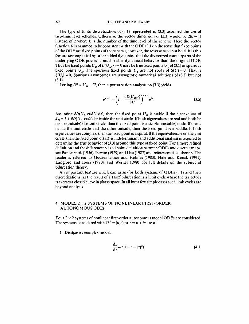
1. Dissipative complex model:
d2
dt z(i+_. Izl 2) (4.1)

DYNAMICALSTUDYOF SPURIOUS STEADY-STATE NUMERICAL SOLUTIONS 229
2. Damped Pendulum model:
du-- = v (4.2a)dt
du
dt = - ev - sin(u) (4.2b)
3. Predator-Prey model:
du-- = - 3u + 4u 2 - 0.5uv - u 3 (4.3a)dt
dl)-- = - 2.1 v + uv (4.3b)dt
4. Perturbed Hamiltonian System model:
du
_-_ = e(1 - 3u) + ] [1 - 2u + u2 - 2v(1 - u)] (4.4a)
dv
dt -- e(1 - 3v) - ¼[1 - 2v + v2 - 2v(1 - v)] (4.4b)
Here e is the system parameter for (4.1), (4.2) and (4.4).
The perturbed Hamiltonian model can be related to the numerical solution of the
viscous Burgers' equation with no source term
_u I O(u 2) _Zuq /_>o. (4.5)_t 2 & -_'_-_x_
Let uj(t) represent an approximation to u(xj, t) of (4.5) where xj =jAx, j= 1 .... ,J,with Ax the uniform grid spacing. Consider the three-point central difference in space
Jwith periodic condition us+ i = u_, and assume Zi= 1 u_= constant, which implies that
J_j= i dujdt = 0. If we take J = 3 and Ax = 1/3 then, with _:= 9fl, this system can bereduced to a 2 × 2 system of first-order nonlinear autonomous ODEs (4.4) with
U r = (ul, u2) = (u, v). In this case, the nonlinear convection term is contributing to the
nonlinearity of the ODE system (4.4).
These four equations were selected to bring out the dynamics of numerics for four
different types of solution behavior of the ODEs. The dissipative complex system (4.1)possesses either a unique stable fixed point or limit cycle with an unstable fixed point
depending on the value ofe. This is the rare situation where the analytical expression of
a limit cycle can be found. The purpose of choosing (4.1) is to illustrate the numerical
accuracy of computing a limit cycle and the spurious dynamics associated with this
type of asymptote. The damped pendulum (4.2), arising from modelling of a physicalprocess, exhibits a periodic structure of an infinite number of fixed points. The
predator-prey model (4.3), arising from modelling of biological process, exhibitsmultiple stable fixed points without a periodic pattern as model (4.2). The perturbed
Hamiltonian model (4.4), which arises as a gross simplification of finite discretization of

230 H.C. YEE AND P. K. SWEBY
the viscous Burgers' equation, exhibits an unique stable fixed point. Following the
classification of fixed points of(3.1) in Section III, one can easily obtain the following:
Fixed Point of (4.1): The dissipative complex model has a unique fixed point at
(u, v) = (0, 0) for _:_<0. The fixed point is a stable spiral if;3 < 0. It is a center if_: = 0. For
> 0, the fixed point (0, 0) becomes unstable with the birth of a stable limit cycle with
radius equal to v_ centered at (0, 0). Figure 4.1 shows the phase portrait (u-v plane) of
system (4.1) for _:= - 1 and _:= 1 respectively. Here the entire (u, t_)plane belongs to thebasins of attraction of the stable fixed point (0,0) ife < 0. On the other hand, if c. > 0, the
entire (u, v) plane except the unstable fixed point (0, 0) belongs to the basin of attraction
of the stable limit cycle centered at (0,0).
Fixed Points _" (4.2): The damped pendulum (4.2) has an infinite number of fixed
points, namely (krt, 0) for integer k. Ifk is odd, the eigenvalues of the Jacobian J(UE) are
of opposite sign and these fixed points are saddles. If k is even, however, two cases must
be considered, depending on the value of e.. If _ < 2 and positive, the eigenvalues are
complex with negative real part and the fixed points are stable spirals. If _:_> 2, theeigenvalues are real and negative and the fixed points are nodes. If _:= 0, the spirals
become centers. Figure 4.2 shows the phase portrait and their corresponding basins of
attraction for system (4.2). The different shades of grey regions represent the variousbasins of attraction of the respective stable fixed points for 4:= 0.5 and c = 2.5.
Fixed Points t_f (4.3): The fixed points of the predator-prey equation are less regular
than those for the damped pendulum equation. System (4.3) has four fixed points (0,0),
(0, 1), (3,0) and (2.1, 1.98). By looking at the eigenvalues of the Jacobian of S, one finds
that (0,0) is a stable node, (2.1, 1.98) is a stable spiral, and (1,0) and (3,0) are saddles.
Figure 4.3 shows the phase portrait and their corresponding basins of attraction for
system (4.3). The different shades of grey regions represent the various basins ofattraction of the respective stable fixed points. The white region represents the basin of
3-
2
I
0
-1
-2"
I: =-I
-3 3' ' 12 ................... i1, ,i _, J i- - - 0 1 2 3
U
f=l
I
-2-
,3 2 _ 0 I 2 3
L_
Figure 4.1 Phase Portraits and basins of Attraction Dissipative ('omplex Equation.

DYNAMICAL STUDY OF SPURIOUS STEADY-STATE NUMERICAL SOLUTIONS 231
I_ =0.5
2.5 ....._i!_ii::_J:_ ::i_!,+.....
> o.o- "_: i_i_!i_
-5.0"-2.5 .::_i_::
-10.0 -7.5 -5.0 -2.5 0.0 2.5 5.0 7.5 10.0
U
13 =2.5
-5.0
-_0.0 -7.5 -5.0 -2.5 0.0 2.5 5.0 7.5 10.0
U
Figure 4.2 Phase Portraits and Basins of Altraclion Damped Pendulum Equation.
_._
-I 0 I 2 3 4 5
U
Figure 4.3 Phase Portraits and Basins of Attr:lction Predalor-t_rc+_ Equ_ttitm.
232 H.C. YEE AND P. K. SWEBY
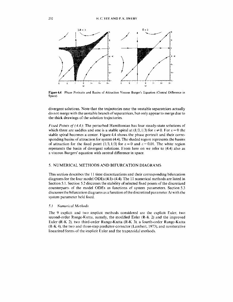
Figure 4.4
Space).
£ r 0 t- £- _-
o
J0='3
0
U
<
"t-
[.-
t- g- [-
Phase Portraits and Basins of Attraction Viscous Burger's Equation (Central Difference in
divergent solutions. Note that the trajectories near the unstable separatrices actually
do not merge with the unstable branch ofseparatrices, but only appear to merge due tothe thick drawings of the solution trajectories.
Fixed Points of(4.4): The perturbed Hamiltonian has four steady-state solutions of
which three are saddles and one is a stable spiral at (1/3, 1/3) for e =/=0. For e = 0 the
stable spiral becomes a center. Figure 4.4 shows the phase portrait and their corre-
sponding basins of attraction for system (4.4). The shaded region represents the basins
of attraction for the fixed point (1/3, 1/3) for e-- 0 and _;-- 0.01. The white region
represents the basin of divergent solutions. From here on we refer to (4.4) also as
a viscous Burgers' equation with central difference in space.
5. NUMERICAL METHODS AND BIFURCATION DIAGRAMS
This section describes the 11 time discretizations and their corresponding bifurcation
diagrams for the four model ODEs (4.1)-(4.4). The 11 numerical methods are listed in
Section 5.1. Section 5.2 discusses the stability of selected fixed points of the discretized
counterparts of the model ODEs as functions of system parameters. Section 5.3discusses the bifurcation diagrams as a function of the discretized parameter At with the
system parameter held fixed.
5.1 Numerical Methods
The 9 explicit and two implicit methods considered are the explicit Euler, twosecond-order Runge-Kutta, namely, the modified Euler (R-K 2j and the improved
Euler (R-K 2), two third-order Runge-Kutta (R-K 3), a fourth-order Runge-Kutta
(R-K 4), the two and three-step predictor-corrector (Lambert, 1973), and noniterative
linearized forms of the implicit Euler and the trapezoidal methods.

DYNAMICAL STUDY OF SPURIOUS STEADY-STATE NUMERICAL SOLUTIONS 233
(1) Explicit Euler (lst-order; R-K 1):
f.+ 1 = U" + rS"; S" = S(U"k (5.1)
(2) Modified Euler (R-K 2):
U _÷1 =U"+rS(U"+2S" ), (5.2)
(3) Improved Euler (R-K 2):
/.
U "÷_ = U" + -_[S _ + S(U + rS")], (5.3)
(4) Heun (R-K 3):
(5) Kutta (R-K 3):
(6) R-K 4:
r
U.+ t = U" +-_(kl +3k3)
k2 =S _
k3=s(v" >k+ 3 2},
t"
U "+t=U"+_(k l+4k2+k 3)
k 3 = S(U" - rk 1 + 2rk2),
r kU "+I=U"+_(l+2k2+2k3+k4)
kl = S"
(5.4)
(5.5)
(5.6)

234 H. C. YEE AND P. K. SWEBY
k 4 = S(U" + rk3),
(7, 8) Predictor-eorrector for m = 2, 3 (PC2, PC3):
U _°_= U" +rS"
r n
U_k+tj=U _ +_2[S + s_k_], k=O,l ..... m-- I
r
U,+I=U"+_[S,+S _m _],
(9) Adam-Bashforth (2nd-order):
/.
u "+' = u" + _ [3s(u") - s(u"- 1)],
(10) Linearized Implicit Euler:
U" + 1 = U" + r(I - rJ")- 1S"
\OU] and det(l -- rJ _) :/= O,
(11) Linearized Trapezoidal:
U"+I--U"+ r(l-2 J")- ' S"
J"=(OS_"\OU] (2r)and det l-zd _0,
(5.7)
15.8)
(5.9)
(5.1ot
where the numeric identifier after the "R-K" indicates the order of accuracy of thescheme and r = At and det( ) means the determinant of the quantity inside the ().
Schemes (10) and (11) are unconditionally stable methods. See Beam and Warming
(1976) and Yee (1989) for the versatility of the linearized implicit Euler and linearized
trapezoidal methods in CFD applications. A comparison between Newton method in
solving the steady part of the ODEs and the linearized implicit method (5.9) for model
(4.4) is included in Section 6.5. Studies on Newton method in solving the steady state
part of the PDE and some iteration procedures in solving the nonlinear algebraic

DYNAMICAL STUDY OF SPURIOUS STEADY-STATE NUMERICAL SOLUTIONS 235
equation resulting from four implicit LMMs are reported in a separate paper (Yee andSweby 1933a). Although the explicit Euler can be considered as an R-K 1, it is also
a LMM. All of the R-K methods (higher than first order) and the predictor-correctormethods are nonlinear in the parameter space r, and all LMMs are linear in r. As
discussed in Yee et al. (1991), a necessary condition for a scheme to produce spuriousfixed points of period one is the introduction of nonlinearity in the parameter space r. It
can be shown later that this property plays a major role on the shapes and sizes of the
associated numerical basins of attraction of the scheme. For simplicity in referencing,
hereafter we use "implicit Euler" and "trapezoidal" to mean the linearized forms (5.9)and (5.10), respectively, unless otherwise stated.
5.2 Stability of Fixed Points of Numerical Methods as a Function of SystemParameters
In our later study, we assume a fixed system parameter so that only the discretized
parameter comes into play. However, in order to get a feel for the numerical stability of
these schemes around selected stable fixed points U E as a function of the system param-
eter e, Figures 5.1-5.3 show the stability regions of the schemes as a function of the
s- R-K 1
4"
3"
2"
--S -4 -3 -2 -1 0 I 2
£
5-
4-
3-
2-
1-
0
-S
R-K2
-4 -3 -2 -1 0 1 2
£
l R-K3 i R-K4
o , _ f i ' ' i T i , i- , _ _ r i _ T !
-5 4 -3 -2 -1 0 1 2 -S --4 -3 -2 -1 0 1 2
£ £
Figure 5.1 Stability Regions vs. System Parameters Dissipative Complex Equation.
236 H.C. YEE AND P. K. SWEBY
pc2-5 -4 -3 -2 -1 0 1 2
(
Pc3-5 4 -3 -2 -I 0
(
Ad.ms. .sh,o h-5 -4 -3 -2 -1 0 ! 2
(
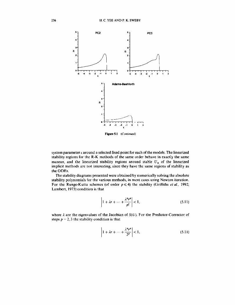
Figure 5.1 (Continued)
I , I
1 2
system parameter e around a selected fixed point for each of the models. The linearizedstability regions for the R-K methods of the same order behave in exactly the same
manner, and the linearized stability regions around stable U_ of the linearized
implicit methods are not interesting, since they have the same regions of stability asthe ODEs.
The stability diagrams presented were obtained by numerically solving the absolute
stability polynomials for the various methods, in most cases using Newton iteration.
For the Runge-Kutta schemes (of order p _<4) the stability (Grifliths et ai., 1992;Lambert, 1973) condition is that
_ Pr p [
1 + _.r + ..- +-_-.v <1,(5.11)
where 2 are the eigenvalues of the Jacobian of S(U). For the Predictor-Corrector of
steps p = 2, 3 the stability condition is that
I ,_PrpII +).r + -.. +_- <1,(5.ll)
DYNAMICAL STUDY OF SPURIOUS STEADY-STATE NUMERICAL SOLUTIONS 237
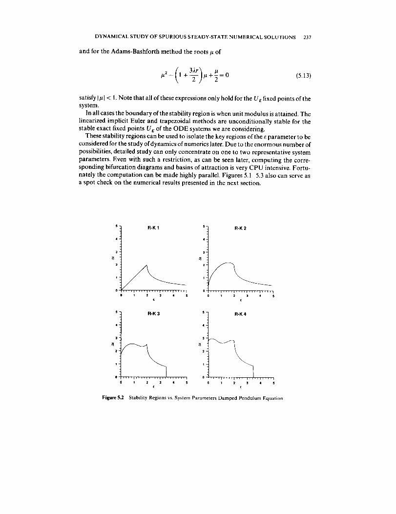
and for the Adams-Bashforth method the roots p of
/_2- I+T//_+_=o(5.13)
satisfy [_[ < 1. Note that all of these expressions only hold for the U e fixed points of thesystem.
In all cases the boundary of the stability region is when unit modulus is attained. The
linearized implicit Euler and trapezoidal methods are unconditionally stable for thestable exact fixed points U e of the ODE systems we are considering.
These stability regions can be used to isolate the key regions of the e parameter to beconsidered for the study ofdynamics of numerics later. Due to the enormous number of
possibilities, detailed study can only concentrate on one to two representative system
parameters. Even with such a restriction, as can be seen later, computing the corre-
sponding bifurcation diagrams and basins of attraction is very CPU intensive. Fortu-nately the computation can be made highly parallel. Figures 5.1 5.3 also can serve as
a spot check on the numerical results presented in the next section.
0 I 2 3 4 5 0 1 2 3 4 S
( I[
S-
4-
3-
2
I
0
R-K 3
%,, ,,,i ir1,111_ I
1 2 3 4 5
(
S
4
3
2
R-K4
,it, r],lr,rr_ I
1 2 3 4 5
(
Figure 5.2 Stability Regions vs. System Parameters Damped Pendulum Equation.

238 H.C. YEE AND P. K. SWEBY
o i_,lF;,i,llrl, I
0 1 2 3 4 5
E
5--
4.-
3_
PC3
_r,,,I,,,,I,F,r ]
1 2 3 4 5
£
5--
4"
3"
2"
1
0
0
Adams-Bashforth
I,tll_r_llll_lllt IIIp,I I
1 2 3 4 5
E
Figure 5.2 (Continued)
5.3 Bifurcation Diagrams
In this section, we show the bifurcation diagrams of selected R-K methods. It illus-
trates some of the many ways in which the dynamics of a numerical discretization
of 2 x 2 first-order autonomous nonlinear system of ODEs can differ from the
system itself. Note that there is no limit cycle or higher dimensional tori counter-
part for the scalar first-order autonomous ODEs. Spurious limit cycles and higher
dimensional tori can only be introduced by the numerics when solving nonlinearODEs other than scalar first-order autonomous ODEs (if 2-time level schemes are
used) and/or by using a scheme with higher than two-time level for the scalar first-order autonomous ODEs. |n Section Vl, we showed how numerical basins of attrac-
tion can complement the bifurcation diagrams in gaining more detailed global
asymptotic behavior of numerical schemes. We purposely present our results in
this order (not showing the basins of attraction) in order to bring out the importanceof basins of attraction for the time-dependent approach in obtaining steady-statenumerical solutions.
Even though the analytical solutions of the these models are known, depending on
the scheme, the dynamics of their discretized counterparts might be very difficult to
analyze. In particular, some analytical linearized analysis (without numerical computa-
tions) of fixed points of periods one and two is possible for the predator-prey and the
damped pendulum case. However, analytical analysis for the dissipative complex

DYNAMICAL STUDY OF SPURIOUS STEADY-STATE NUMERICAL SOLUTIONS 239
model and the perturbed Hamiltonian is not practical. For a detailed analysis of these
selected cases, readers are referred to Sweby and Yee (1991). For the majority of the cases
where rigorous analysis is impractical we study the dynamics of numerics using numericalexperiments.
Note that some global solution behavior of fixed points of the nonlinear discretized
equations (5.1) (5.10) for (4.1) (4.4) can be obtained by the pseudo arclength continua-tion method devised by Keller (1977), a standard numerical method for obtaining
bifurcation curves in bifurcation analysis. A major shortcoming of the pseudo arclength
continuation method is that for problems with complicated bifurcation patterns, it
cannot provide the complete bifurcation diagram without known start up solutions
for each of the main bifurcation branches before one can continue the solution along
a specific main branch. For spurious asymptotes it is usually not easy to locate even justone solution on each of these branches.
The nature of our calculations requires thousands of iterations of the same equation
with different ranges of initial data on a preselected (u, v) domain and range of thediscretized parameter space At. Since the NASA Ames CM-2 allows vast numbers
(typically 65,536) of calculations to be performed in parallel, our problem is perfect forcomputation on the CM-2.
5-
4 ¸
3
2
1
0
0
R-K 1
,Jqfllllfl_f_llrrll_r_l I
t 2 3 4 5
g
0 1 2 3 4 5
£
5-
4
3
2
1
0
0
R-K 3
_l_rilfTf11TIPl'',Jt,,qf I
1 2 $ 4 5
[
5-
4-
3"
2
1"
0
0
R-K4
f,f Jl_l , ,11111¢_,1 iTll_l I
1 2 3 4 5
£
Figure 5.3 Stability Regions vs. System Parameters Viscous Burgers' Equation (Central Difference inSpace).

240 H.C. YEE AND P. K. SWEBY
O_T''r;f'FIIT=;lllllJl'llll
0 1 2 3 4 5
£
PC30 1 2 3 4 5
E
5_
4
3
2
1
0
Adams-Bashlorlh
Illlllll¢llrllllll_lrTIl I
1 2 3 4 5
Figure 5.3 (Continued)
To obain a "full" bifurcation diagram, the domain of initial data and the range of the
At parameter are typically divided into 512 equal increments. For each initial datumand At, the discretized equations are preiterated 3,000-- 5,000 (more or less depending
on the ODE and scheme) before the next 4,000-6,000 iterations are plotted. The
preiterations are necessary in order for the trajectories to settle to their asymptotic
value. The high number of iterations plotted (overlay on the same plot) is to detect
periodic orbits or invariant sets. Since the results are a three dimensional graph
((At, u, r,)), we have taken slices in a given constant t_- and u-plane in order to enhance
viewing the decrease CPU computations. Note that with this method of computing the
bifurcation diagrams, only the stable branches are plotted. Some of the bifurcation
diagrams in a _' = constant plane for the four model ODEs and for the modified Euler,
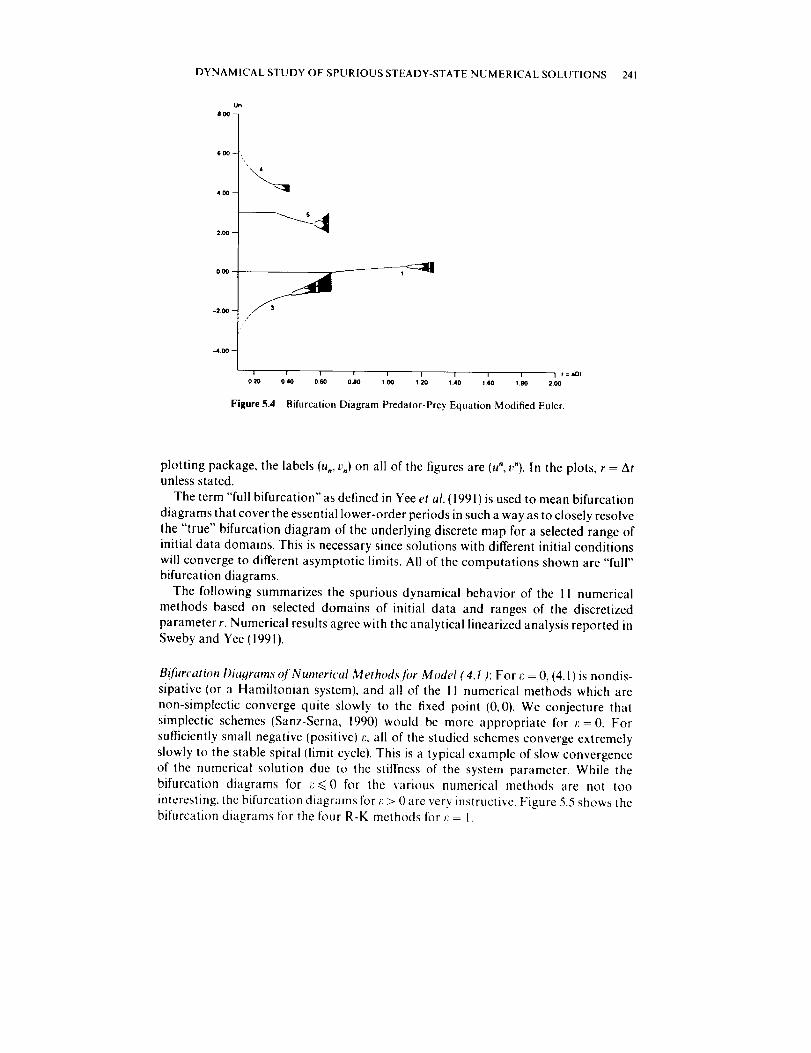
improved Euler, Kutta and R-K 4 methods are shown in Figures 5.4-5.8. Figure 5.4shows a typical example of spurious stable fixed points (branches 3 and 4 on the
diagram) occurring below the linearized stability by the modified Euler method. It also
shows the existence of spurious asymptotes such as limit cycles, higher order periodic
solutions and possibly numerical chaos (chaos introduced by numerics), See later
sections and subsections for further details. Selected bifurcation diagrams for the rest ofthe numerical methods are illustrated in Section IV with basins of attraction
superimposed (see Figures 6.3 6.5,6.13, 6.14, and 6.19 6.20). See also the original
NASA internal report RNR-92-008, March 1992 for additional illustrations. Due to the
DYNAMICAL STUDY OF SPURIOUS STEADY-STATE NUMERICAL SOLUTIONS
tin
800
241
2.00
O0(I
-2,00 --
4.00--
/
I ! I I I I I I i I r=QDI0.20 0.40 0,60 0.80 1.00 1.20 1,40 1,60 1,60 2.00
Figure 5.4 Bifurcation Diagram Predator-Prey Equation Modified Euler.
plotting package, the labels (u,, v,) on all of the figures are (u", v"). In the plots, r = Atunless stated.
The term "full bifurcation" as defined in Yee et al. (1991) is used to mean bifurcation
diagrams that cover the essential lower-order periods in such a way as to closely resolve
the "true" bifurcation diagram of the underlying discrete map for a selected range ofinitial data domains. This is necessary since solutions with different initial conditions
will converge to different asymptotic limits. All of the computations shown are "full"bifurcation diagrams.
The following summarizes the spurious dynamical behavior of the 11 numerical
methods based on selected domains of initial data and ranges of the discretized
parameter r. Numerical results agree with the analytical linearized analysis reported inSweby and Yee (1991).
B!fureation Diaqrams of Numerical Methods lot Model (4.1): For _:= 0, (4.1) is nondis-sipative (or a Hamiltonian system), and all of the I ! numerical methods which are
non-simplectic converge quite slowly to the fixed point (0,0). We conjecture that
simplectic schemes (Sanz-Serna, 1990) would be more appropriate for _:=0. For
sufficiently small negative (positive) ,:, all of the studied schemes converge extremely
slowly to the stable spiral (limit cycle). This is a typical example of slow convergenceof the numerical solution due to the stiffness of the system parameter. While thebifurcation diagrams for _:_<0 for the various numerical methods are not too
interesting, the bifurcation diagrams for _:> 0 are very instructive. Figure 5.5 shows thebifurcation diagrams for the four R-K methods for _:= I.
242 H.C. YEE AND P. K. SWEBY
3.0
0.0-
U n
Modified Euler
u n
J
,/
\
o15 ,is ='s
30
2.0
, 0.0
urt
Improved Euler
o15 ,is 215r=a[
Kutta
_:_ 3,'5 ,:5 '
Un4.
3
2.
1
R-K 4
1 2
r=a_
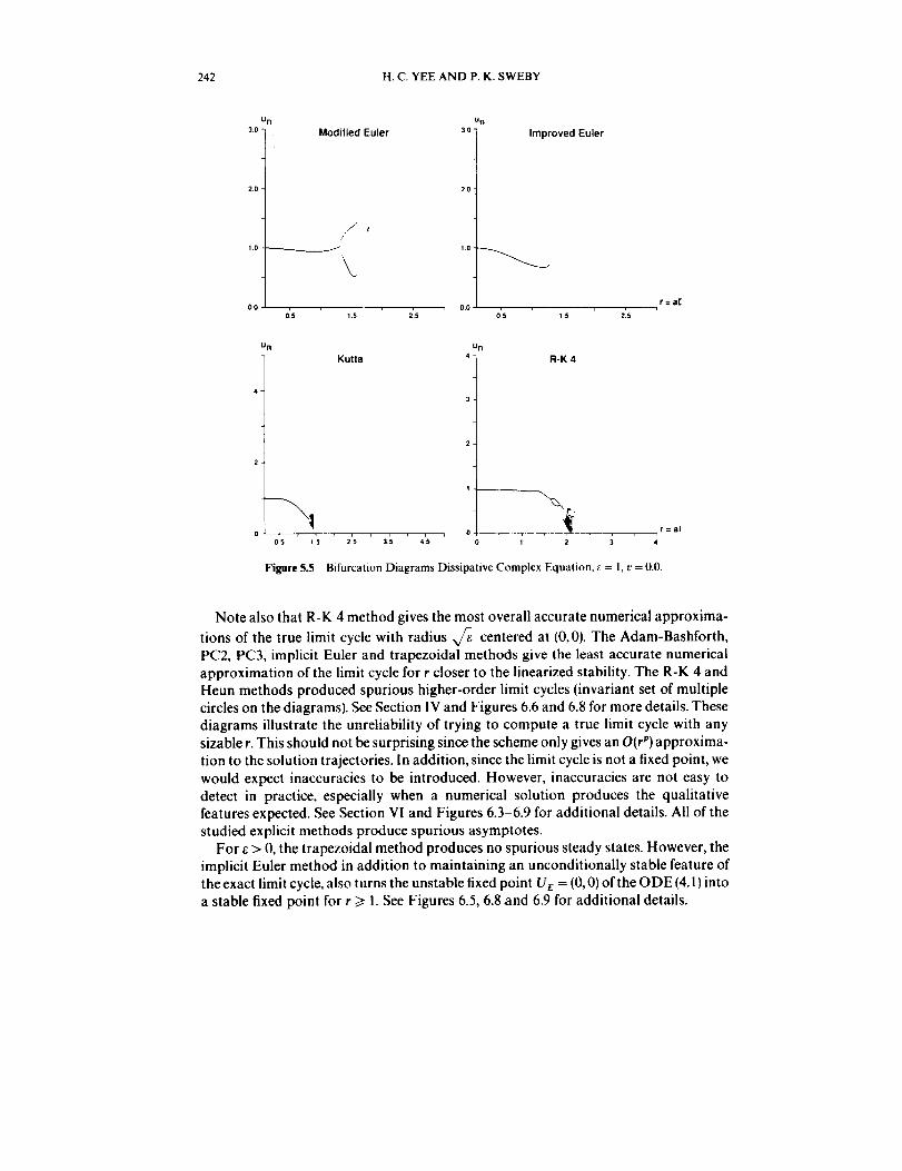
Figure 5.5 Bifurcation Diagrams Dissipative Complex Equation, e = 1, v = 0.0.
Note also that R-K 4 method gives the most overall accurate numerical approxima-
tions of the true limit cycle with radius x/_ centered at (0,0). The Adam-Bashforth,PC2, PC3, implicit Euler and trapezoidal methods give the least accurate numerical
approximation of the limit cycle for r closer to the linearized stability. The R-K 4 andHeun methods produced spurious higher-order limit cycles (invariant set of multiplecircles on the diagrams). See Section IV and Figures 6.6 and 6.8 for more details. Thesediagrams illustrate the unreliability of trying to compute a true limit cycle with anysizable r. This should not be surprising since the scheme only gives an O(rp)approxima-tion to the solution trajectories• In addition, since the limit cycle is not a fixed point, wewould expect inaccuracies to be introduced• However, inaccuracies are not easy todetect in practice, especially when a numerical solution produces the qualitativefeatures expected. See Section VI and Figures 6.3-6•9 for additional details. All of thestudied explicit methods produce spurious asymptotes.
For e > 0, the trapezoidal method produces no spurious steady states• However, theimplicit Euler method in addition to maintaining an unconditionally stable feature ofthe exact limit cycle, also turns the unstable fixed point U_ = (0, 0) of the ODE (4. l) intoa stable fixed point for r/> l. See Figures 6.5, 6.8 and 6.9 for additional details.
DYNAMICAL STUDY OF SPURIOUS STEADY-STATE NUMERICAL SOLUTIONS 243
8
6
4
2
0
u n
5-
4_
3
2
Modified EulerUn Un Improved Euler5-
4
3
2
1-
f21o 21, 2'8 o lle 2:0 21,
t=a
Un
5-
4.
3
2
1
r r , _ 0 ,
16 20 ' 214 ' 218 15 2;0 25
Kutta R-K 4
r=a[
30 3'5
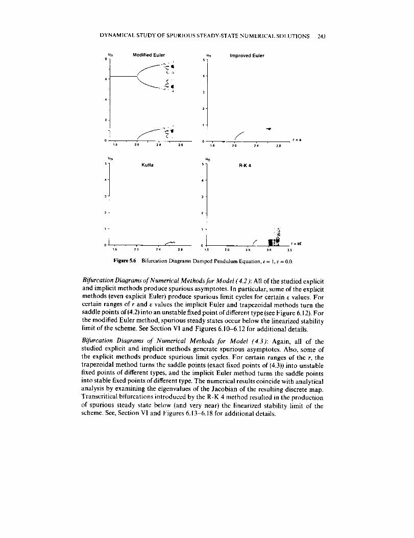
Figure 5.6 Bifurcation Diagrams Damped Pendulum Equation, e = 1, v = 0.0.
Bifurcation Diagrams of Numerical Methods for Model (4.2): All of the studied explicit
and implicit methods produce spurious asymptotes. In particular, some of the explicitmethods (even explicit Euler) produce spurious limit cycles for certain e values. For
certain ranges of r and e values the implicit Euler and trapezoidal methods turn the
saddle points of (4.2) into an unstable fixed point of different type (see Figure 6.12). For
the modified Euler method, spurious steady states occur below the linearized stabilitylimit of the scheme. See Section Vl and Figures 6.10-6.12 for additional details.
Bifurcation Diagrams of Numerical Methods for Model (4.3): Again, all of the
studied explicit and implicit methods generate spurious asymptotes. Also, some ofthe explicit methods produce spurious limit cycles. For certain ranges of the r, the
trapezoidal method turns the saddle points (exact fixed points of (4.3)) into unstable
fixed points of different types, and the implicit Euler method turns the saddle points
into stable fixed points of different type. The numerical results coincide with analytical
analysis by examining the eigenvalues of the Jacobian of the resulting discrete map.Transcritical bifurcations introduced by the R-K 4 method resulted in the production
of spurious steady state below (and very near) the linearized stability limit of thescheme. See, Section V1 and Figures 6.13 6.18 for additional details.
244 H.C. YEE AND P. K. SWEBY
U n
1 Modified Euler
/
o AA
0.2 0.6 1.0 1.4
U n
Improved Euler
118 ' -1 , , , , , ,r = aD!02 0.6 1.0 1:4 1:8
U n
4
2
1
0
-1
02 016
KuttaU n
4 R-K 4
3
\ ,
2
1
0
10 1.4 1:8 -I 0:2 0.6 _.0 I 4 IS r = aDt
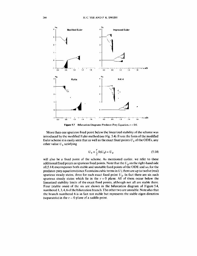
Figure 5.7 Bifurcation Diagrams Predator-Prey Equation, t,,= 0.0.
More than one spurious fixed point below the linearized stability of the scheme was
introduced by the modified Euler method (see Fig. 5.4). From the form of the modifiedEuler scheme it is easily seen that as well as the exact fixed points U E of the ODEs, any
other value U s satisfying
r
Us + -}S(Us) = Ur, (5.14)
will also be a fixed point of the scheme. As mentioned earlier, we refer to these
additional fixed points as spurious fixed points. Note that the Ue on the right-hand sideof(5.14) encompasses both stable and unstable fixed points of the ODE and so, for the
predator-prey equations (since S contains cubic terms in U), there are up to twelve (real)spurious steady states, three for each exact fixed point U E. In fact there are six such
spurious steady states which lie in the v = 0 plane. All of them occur below the
linearized stability limits of the exact fixed points, although not all are stable there.Four (stable ones) of the six are shown in the bifurcation diagram of Figure 5.4,
numbered 1, 3, 4, 6 of the bifurcation branch. The other two are unstable. Note also that
the branch numbered 6 is in fact not stable but represents the stable eigen-direction
(separatrix) in the t' = 0 plane of a saddle point.

DYNAMICAL STUDY OF SPURIOUS STEADY-STATE NUMERICAL SOLUTIONS 245
u n
1.5"
I0-
05
O0
-1005
Modified EulerU n
15
1.0
05"
00-
_5-
r = aDt7
-1005 ' '10 i 5 20 25 30 10 Is 2r0 2r5 30
Improved Euler
U n
15
1:0
05
O0
_5
1005
U n
Kutta _5 _ R-K 4/
0.5
t
10 15 2'0 2'5 310 -1015 20 25 30
r = aDt
35
Figure5.8 Bifurcation Diagrams Viscous Burgers" Equation, t:=0,1, r=0.333 (Central Difference inSpace).
B!J'urcation Diayrams of Numerical Methods for Model (4.4): For _:= 0, the ODE (4.4) is
nondissipative and thus for small r, slow convergence was experienced. For r beyondthe iinearized limit and with e, = 0 all of the explicit methods produce spurious limit
cycles. For c,> 0 (and not too large) all of the studied 11 explicit and implicit methods
produce spurious asymptotes. Also, all of the explicit methods produce spurious limit
cycles. For t:=0.1, the Kutta and Heun methods introduce spurious asymptotes(higher than period one) that are below the linearized stability limit of the scheme. SeeFigures 6.19 6.25 for additional details.
6, BASINS OF ATTRACTION AND BIFURCATION DIAGRAMS
This section illustrates how basins of attraction can complement the bifurcation
diagrams in gaining more detailed global asymptotic behavior of time discretizations
246 H.C. YEE AND P. K. SWEBY
for nonlinear DEs. Two different representations of the numerical basins of attrac-tion were computed on the NASA Ames CM-2. One representation is bifurcation
diagrams as a function of At with numerical basins of attraction superimposed on
a constant v- or u-plane. The other representation is the numerical basins of attraction
with stable asymptotes superimposed on the phase plane (u,_'). Before discussing
numerical results for each of the model ODEs, the next subsection gives some
preliminaries on how to compute and on how to interpret the basins of attraction
diagrams for the CM-2.
6.1 Introduction
To obtain a bifurcation diagram with numerical basins of attraction superimposed on
the CM-2, the preselected domain of initial data on a constant v- or u-plane and the
preselected range of the At parameter are divided into 512 equal increments. Again, for
the bifurcation part of the computations, with each initial datum and At, the discretized
equations are preiterated 3,000 5,000 steps before the next 5,000 iterations (more orless depending on the problem and scheme) are plotted. The bifurcation curves appear
on the figures as white curve, white dot and white dense dots. While computing the
bifurcation diagrams it is possible to overlay basins of attraction for each value of At
used. For the numerical basins of attraction part of the computation with each value of
At used, we keep track of where each initial datum asymptotically approaches and
color code them (appearing as a vertical strip) according to the individual asymptotes.While efforts were made to match color coding of adjacent strips on the bifurcation
diagram, it was not always practical or possible. Care must therefore be taken when
interpreting these overlays.
For the basins of attraction on the phase plane (u,v) with selected values of At
and the stable asymptotes superimposed, the (u,v) domain is divided into 512 × 512
points of initial datum. With each initial datum and the selected At, we preiteratethe respective discretized equation 3,000-5,000 steps and plot the next 5,000 steps
to produce the asymptotes. Again, for the basins of attraction part of the compu-tations, for each value of At used, we keep track of where each initial datum
asymptotically approaches and color code them according to the individual asym-
ptotes. All of the selected time steps At shown are based on the bifurcation diagram
with the basins of attraction superimposed. The chosen time steps were selected
to illustrate special features of the different bifurcation phenomena on the (u,v)plane. Details of the techniques used for detection of asymptotes and basins of
attraction are given in the appendix of Sweby and Yec (1991). Note that in all of
the plots, ifcolor printing is not available, the different shades of grey represent differentcolors.
As a prelimiary, and before discussing our major results, we discuss the numerical
basins of attraction associated with modified Euler, improved Euler, Kutta and R-K 4
methods for the two scalar first-order autonomous nonlinear ODEs studied in part I of
our companion paper (Yee et al., 1991). The two scalar ODEs are:
du=au{l ul (6.11
dt

DYNAMICAL STUDY OF SPURIOUS STEADY-STATE NUMERICAL SOLUTIONS 247
and
du
dt = au(1 - u)(0.5 - u). (6.2)
The fixed points for (6.1) with a>0 are u=0 (unstable) and u = 1 (stable), and noadditional higher order periodic fixed points or asymptotes exist. The basin of attraction
for the stable fixed point u = 1 is the entire positive plane for all values ofa > 0.
The fixed points for (6.2) with a > 0 are u = 0 (unstable), u = 1 (unstable) and u = 0.5
(stable) and no additional higher-order periodic solutions or asymptotes exist. The
basin of attraction for the stable fixed point u = 0.5 is 0 < u < 1for all a > 0. The white
curve, white dots and white dense dots of Figures 6.1 and 6.2 show the bifurcation
diagrams for four of the R-K methods for (6.1) and (6.2). For more details of the dynamicsof numerics for systems (6.1) and (6.2), see Yee et al. (1991). Intuitively, in the presence of
spurious asymptotes the basins of the true stable steady states can be separated by the
numerical basins of attraction of the stable and unstable spurious asymptotes.Take, for example, the ODE (6.1) where the entire domain u is divided into two basins
of attraction for the ODE independent of any real a. Now if one numerically integrates
the ODE, depending on the scheme and r, extra stable and unstable fixed points of any
order can be introduced by the scheme. The bifurcation part of Figures 6.1 and 6.2,
cannot distinguish the types of bifurcation and the periodicity of the spurious fixed
points of any order. With the numerical basins of attraction and their respective
bifurcation diagrams superimposed on the same plot, the type of bifurcation and towhich initial data asymptote to which stable asymptotes become apparent. Note thatfor Figures 6.1 and 6.2 r = aAt.
For example, any initial data residing in the green region in Figure 6.1 for the
modified Euler method belong to the numerical basin of attraction of the spurious(stable) branch emanating from u = 3 and r = 1. Thus, if the initial data is inside the
green region, the solution can never converge to the exact steady state using evena small fixed but finite At (all below the linearized stability limit of the scheme). Note
that the green region extends upward as r decreases below 1.Thus for certain ranges of
r wdues, the domain is divided into four basins (instead of two for the ODE). But of
course higher period spurious fixed points exist for other ranges of r and more basinsare created within the same u domain.
A similar situation exists for the R-K 4 method (Fig. 6.1 ), except now the numerical
basins of attraction of the spurious fixed points occur very near the linearized stabilitylimit of the scheme, with a small portion occurring below the linearized stability limit.
In constrast to the improved Euler method (Fig. 6.1), the green region represents thenumerical basins of one of the spurious stable transcritical bifurcation branches of the
fixed point. The bifurcation curve directly below it with the corresponding red portion
is the basin of the other spurious branch. See Yeeet al. (1991)or Hale and Kocak (1991)
for a discussion of the different types of bifurcations. With this way of color coding thebasins of attraction, one can readily see (from the plots) that for ODE (6. I), the modified
Euler, improved Euler and R-K 4 methods, experience one steady bifurcation beforea period doubling bifurcation occurs (Fig. (6.1)). Using the PC3 method to solve (6.1)
(figure not shown: see Yee et al., 1991), more than one consecutive steady bifurcation
occurs before period doubling bifurcation. For ODE (6.21),the improved Euler experi-

248 H C. YEE AND P. K SWEBY
Fil,ture 6.1 (Sec ('olor Plate I at the back of lhi,, issue I
ences two consecutive steady bifurcations before a period doubling bifurcation occurs
(Fig. [6.2)). Using the PC3 method to solve (6.2)[figure not shown: see Yee et al. 1991 _,
four consecutive steady bifurcations occur before period doubling bifurcations. The
modified Euler and R-K 4 methods, however, experience only one steady bifurcation
before period doubling bifurcations occur.

DYNAMICAL STUDY OF SPURIOUS STEADY-STATE NUMERICAL SOLUTIONS 249
Figure 6.2 tSee Color Plate II at the back of this issuc.)
The next section presents similar diagrams for the 2 × 2 systems of model nonlinear
ODEs [4.1) [4.4). In this case, only basins of attraction with bifurcation diagrams
superimposed on t, = constant planes are shown. Selected results for both representa-tions of numerical basins of attraction are shown in Figures 6.3 6.5, 6.8 6.25 for the
numerical methods. Section 6.6 summarizes similar results presented in Yee and

250 H.C. YEE AND P. K. SWEBY
Sweby (1993a) for iterative procedures in solving nonlinear systems of algebraic
equations arising from four implicit LMMs. In the plots r = At. White dots and white
curves on the basins of attraction with bifurcation diagrams superimposed representthe bifurcation curves. White dots and white closed curves on the basins of attraction
with the numerical asymptotes superimposed represent the stable fixed points, stable
periodic solutions or stable limit cycles. The black regions represent divergentsolutions.
Note that the streaks on some of plots are either due to the non-settling of the
solutions within the prescribed number of preiterations or the existence of small
isolated spurious asymptotes. Due to the high cost of computation, no further
attempts were made to refine their detailed behavior since our purpose was to show
how, in general, the different numerical methods behave in the context of nonlinear
dynamics.
6.2 Numerical results ]br the Dissipative Complex Equation
Figures 6.3-6.5, 6.8, 6.9 show selected results for the two representations of numerical
basins of attraction for model (4.1) for e = 1. The exact solution for (4.1) with e -- 1 is
a stable limit cycle with unit radius centered at {0, 0). The basin ofattraction for the limit
cycle is the entire (u, v} plane except the unstable fixed point (0, 0).
Comparing Figures 6.3-6.5 with Figure 5.5, one can appreciate the added informa-
tion that the basin of attraction diagrams can provide. As At moves closer to the
linearized stability limit of the limit cycle, the size (red) of the numerical basins ofattraction decreases rapidly. This is due to the existence of spurious unstable asym-
ptotes below as well as above the linearized stability limit. The green region, shown in
Figure 6.5 using the implicit Euler method, is the numerical basin of attraction for the
stabilized fixed point (0,0). Note how the implicit Euler method turns an unstable fixed
point (0, 0) of the ODE system into a stable one for At >_ I.
Figures 6.6 and 6.7 show the phase trajectories and Figures 6.8 and 6.9 show the
same figures with numerical basins of attraction superimposed for four different At bythe R-K 4 and implicit Euler methods, respectively. Note how little information
Figures 6.6 and 6.7 can provide as compared to Figures 6.8 and 6.9. Note also how
rapidly the size of the basin (red) decreases as At increases for the R-K 4 method. This
phenomenon can relate to practical computations where only a fraction of the
allowable linearized stability limit of At is safe to use if the initial data is not known. For
At = 1.75 and 2, spurious limit cycles of higher order period exist. (The multiple white
circles with only one distinct basin of attraction). In this case, the red regions representthe basins of the spurious numerical solutions.
Figure 6.9 illustrates the situation where unconditionally stable LM M schemes can
converge to a wrong solution if one picks the initial data inside thc green region which
are valid physical initial data for the ODE. Thus even though LM M preserved the same
number of fixed points as the underlying ODE, these lixed points can change type
and stability. This phenomenon is related to the "non-robustness'" of implicit methods
sometimes experienced in CFD computations. In this type of computation where the
initial data are not known, the highest probability of avoiding spurious asymptotes is
achieved when a fraction of the allowable linearized stability limit of At is employed.
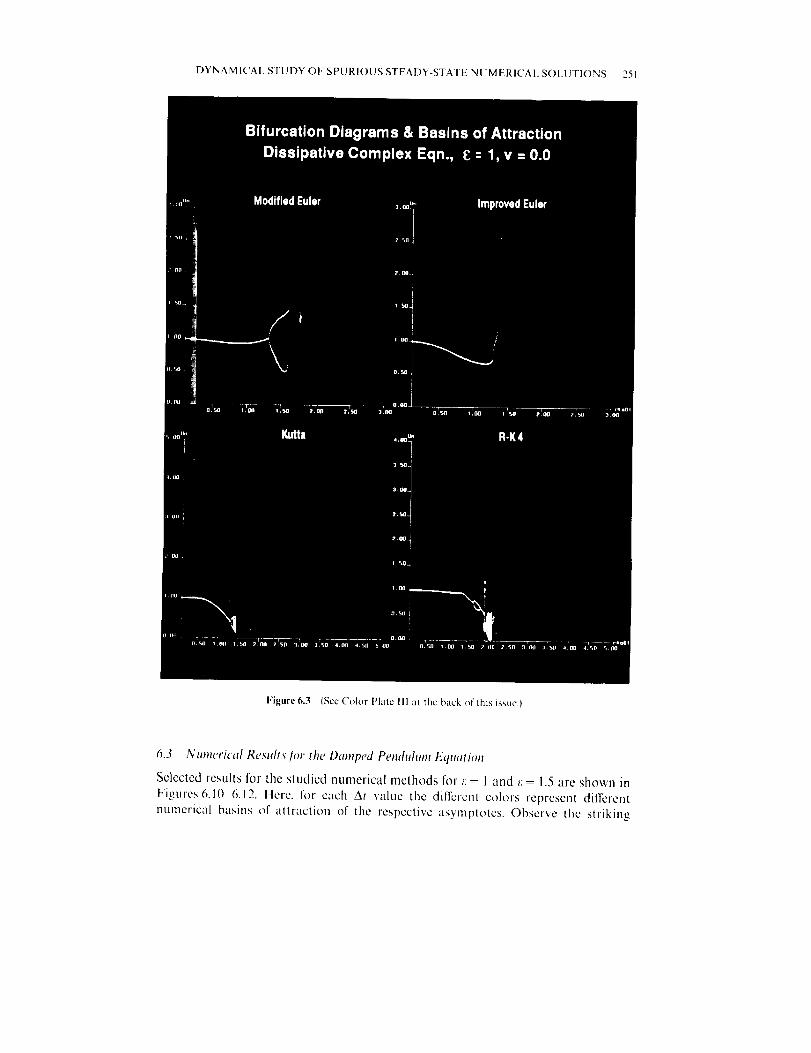
DYNAMICAL STUDY O1: SPURIOUS STEADY-STATE NUMERICAl. SOI.UTIONS 251
F'il_ure6.3 {See Color Plate Ill at the back of lllis issue.I
6.3 Numerical Re.sults.[m" the Damped Pemlulum Equation
Selccted results for the studied ntunerical melhods for }:= 1 and }:= 1.5 are shown in
F'igures6.10 6.12. Here, for each At value the different colors represent different
numerical basins of attraction of the respective asymptotes. Observe the striking
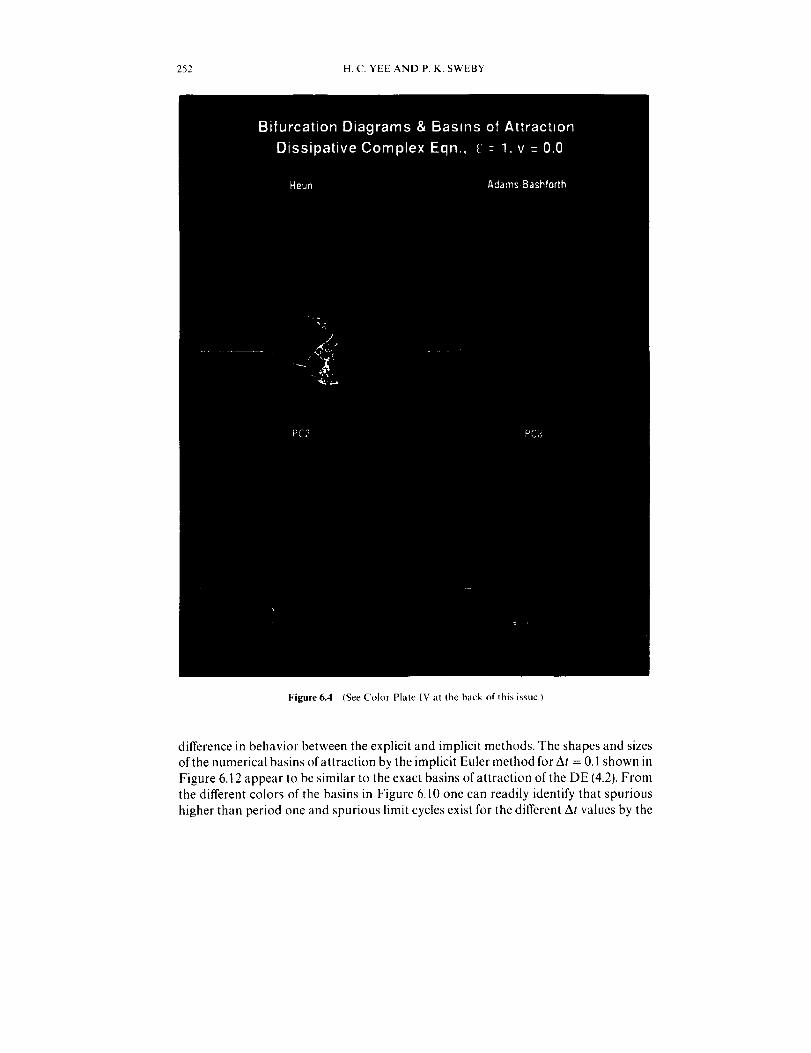
252 H.C. YEE AND P. K. SWEBY
Figure 6.4 (See Color Plate IV at the back of this issue.)
difference in behavior between the explicit and implicit methods. The shapes and sizesof the numerical basins of attraction by the implicit Euler method for At = 0.1 shown in
Figure 6.12 appear to be similar to the exact basins of attraction of the DE (4.2). Fromthe different colors of the basins in Figure 6.10 one can readily identify that spurious
higher than period one and spurious limit cycles exist for the different At values by the
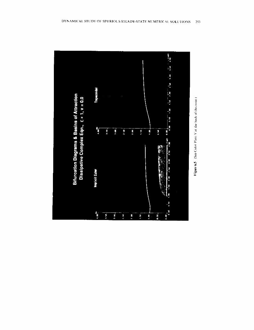
DYNAMICAl. STUDY OF SPURIOUS STEADY-STATE NUMERICAl. SOLUTIONS 253
v
k_
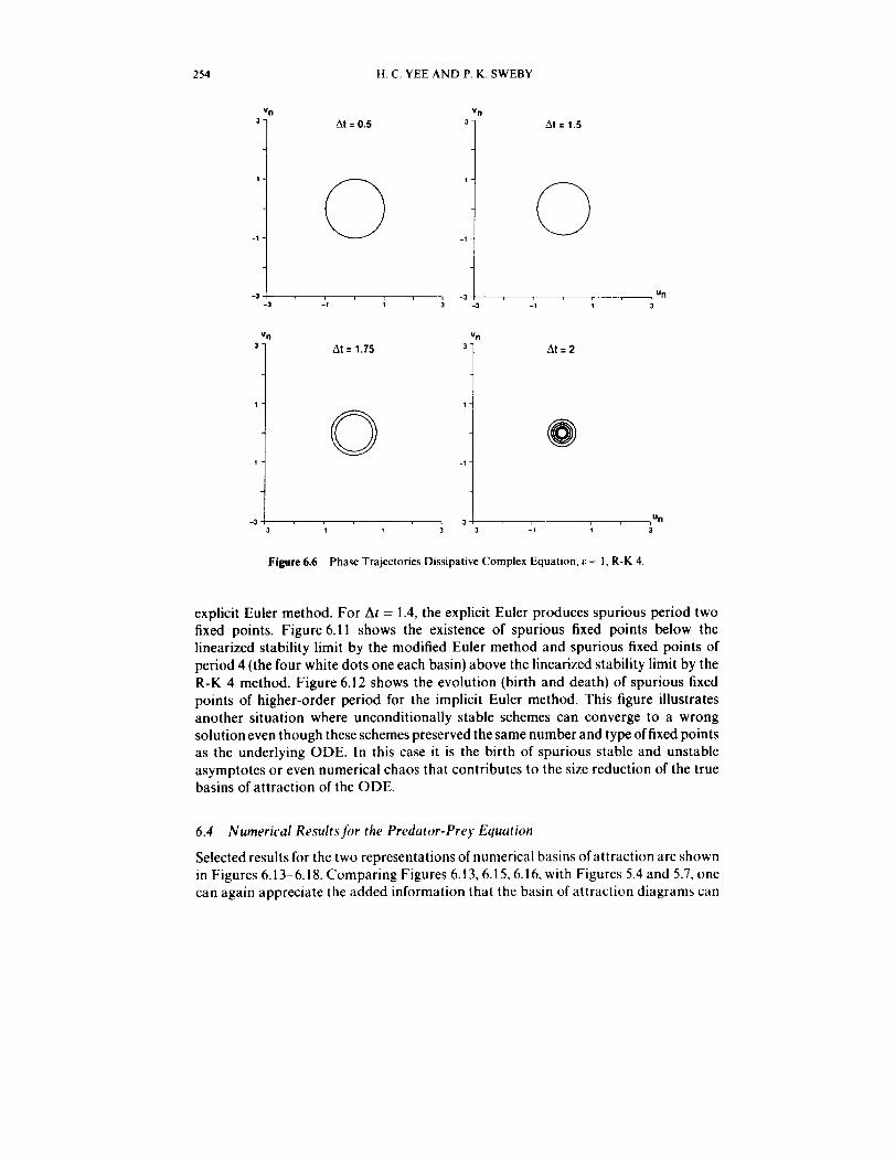
254 H.C.YEEANDP.K.SWEBY
Vn
3-
-3-3
Vn
3
-3
At = 0.5
v n
3- At = 1,S
-3 -1 1 3
At = 1.75
©
vrl
3 At = 2
1
@-1
, , r ,-1 1 3 -3 , Url-3 -1 1 3
Figure 6.6 Phase Trajectories Dissipative Complex Equation, _: = I, R-K 4.
explicit Euler method. For At = 1.4, the explicit Euler produces spurious period two
fixed points. Figure 6.11 shows the existence of spurious fixed points below the
linearized stability limit by the modified Euler method and spurious fixed points of
period 4 (the four white dots one each basin) above the iinearized stability limit by the
R-K 4 method. Figure 6.12 shows the evolution (birth and death) of spurious fixed
points of higher-order period for the implicit Euler method. This figure illustratesanother situation where unconditionally stable schemes can converge to a wrong
solution even though these schemes preserved the same number and type offixed points
as the underlying ODE. In this case it is the birth of spurious stable and unstable
asymptotes or even numerical chaos that contributes to the size reduction of the truebasins of attraction of the ODE.
6.4 Numerical Results fi)r the Predator-Prey Equation
Selected results for the two representations of numerical basins of attraction are shown
in Figures 6.13 6.18. Comparing Figures 6.13, 6.15, 6.16, with Figures 5.4 and 5.7, one
can again appreciate the added information that the basin of attraction diagrams can
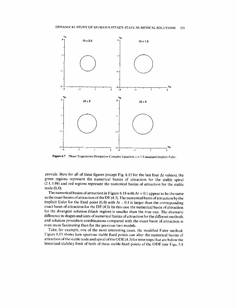
DYNAMICAL STUDY OF SPURIOUS STEADY-STATE NUMERICAL SOLUTIONS 255
VN Vrl
3- 3"At = 0.5 At = 1.5
-3 , -3 Un
Vrl
3- At=2
' @-1
v n
3- At=4
-3 , _ -3 , Un-3 -1 I ; -3 -1 ; 3
Figure 6.7 Phase Trajectories Dissipative Complex Equation, e = 1 Linearized Implicit Euler.
provide. Here for all of these figures (except Fig. 6.15 for the last four At values), the
green regions represent the numerical basins of attraction for the stable spiral(2.1, 1.98) and red regions represent the numerical basins of attraction for the stablenode (0, 0).
The numerical basins of attraction in Figure 6.18 with At = 0.1 appear to be the same
as the exact basins of attraction of the DE (4.3). The numerical basin of attraction by the
implicit Euler for the fixed point (0,0) with At --0.1 is larger than the correspondingexact basin of attraction for the DE (4.3). In this case the numerical basin of attraction
for the divergent solution (black region) is smaller than the true one. The dramatic
difference in shapes and sizes of numerical basins of attraction for the different methods
and solution procedure combinations compared with the exact basin of attraction is
even more fascinating than for the previous two models.
Take, for example, one of the most interesting cases, the modified Euler method.
Figure 6.15 shows how spurious stable fixed points can alter the numerical basins of
attraction of the stable node and spiral of the ODE (4.3) for time steps that are below the
linearized stability limit of both of these stable fixed points of the ODE (see Figs. 5.4
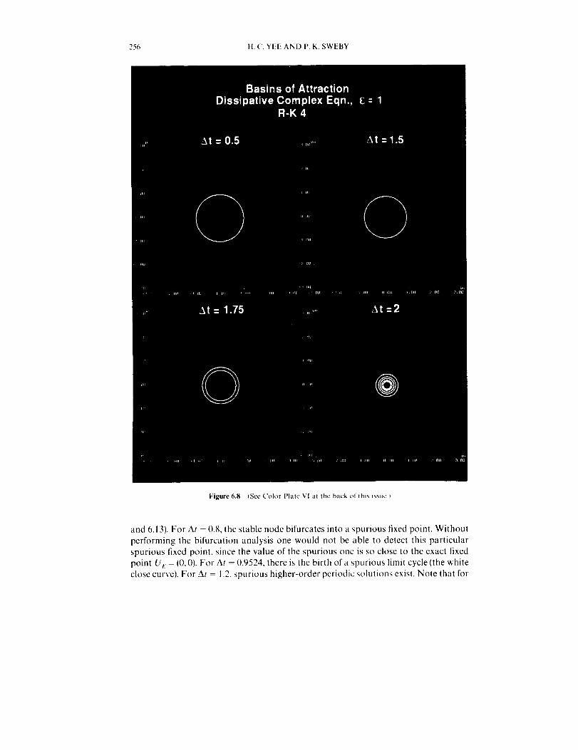
256 H.C. YEE AND P. K. SWEBY
Figure 6.8 (See Color I:'latc VI at the hack of this issue t
and 6.13). For At = 0.8, the stable node bifurcates into a spurious lixed point. Without
performing the bifurcation analysis one would not be able to detect this particular
spurious fixed point, since the value of the spurious one is so close to the exact fixed
point UI; = (0,0). For At = 0.9524, there is the birth of a spurious limit cycle (the white
close curve). For At = 1.2, spurious higher-order periodic solutions exist. Note that for
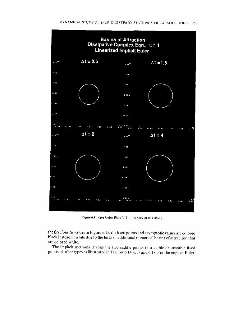
DYNAMICAL STUDY OF SPURIOUS STEADY-STATE NUMERICAL SOLUTIONS 257
Figure 6.9 (See Color Plate VII at the back of this issue.)
the first four At values in Figure 6.15, the fixed points and asymptotic values are coloredblack instead of white due to the birth of additional numerical basins of attraction thatare colored white.
The implicit methods change the two saddle points into stable or unstable fixed
points of other types as illustrated in Figures 6.14, 6.17 and 6.18. For the implicit Euler,
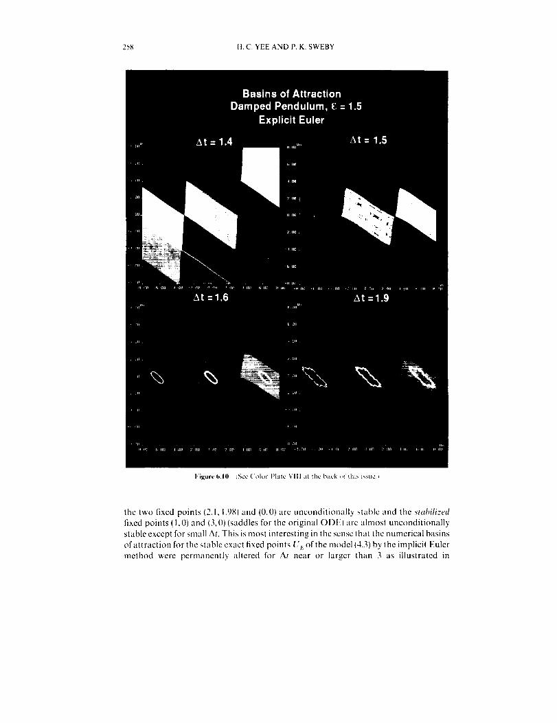
258 H.C. YEE AND P. K. SWEBY
Figure 6.10 (Scc ('olor F'latc VIII at the back of thi_, issuc.l
the two fixed points {2.1, 1.98t and (0,0J are unconditionally stable and the stabilized
fixed points (I,0) and (3,0) (saddles for the original OI)E) are almost unconditionally
stable except for small At. This is most interesting in the sense that the numerical basins
of attraction for the stable exact fixed points U_c of the model (4.3} by the implicit Euler
method were permanently altered for At near or larger than 3 as illustrated in
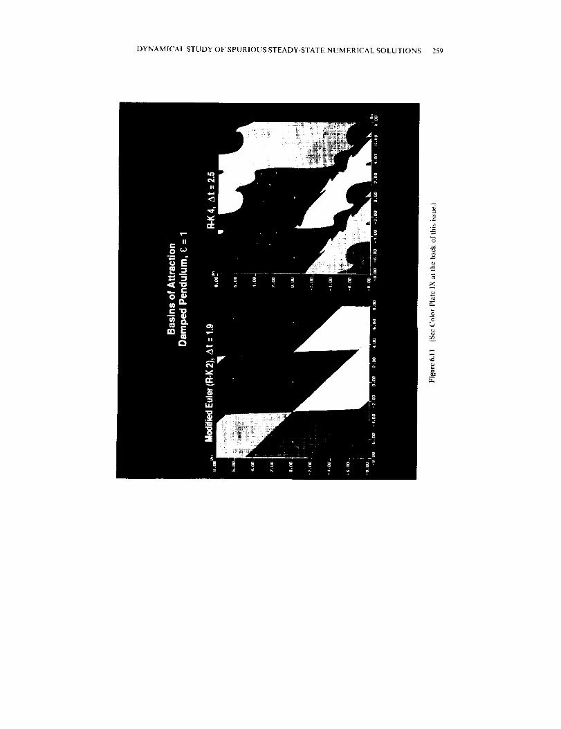
DYNAMICAL STUDY OF SPURIOUS STEADY-STATE NUMERICAL SOLUTIONS 259
A_J
¢o
"6
m
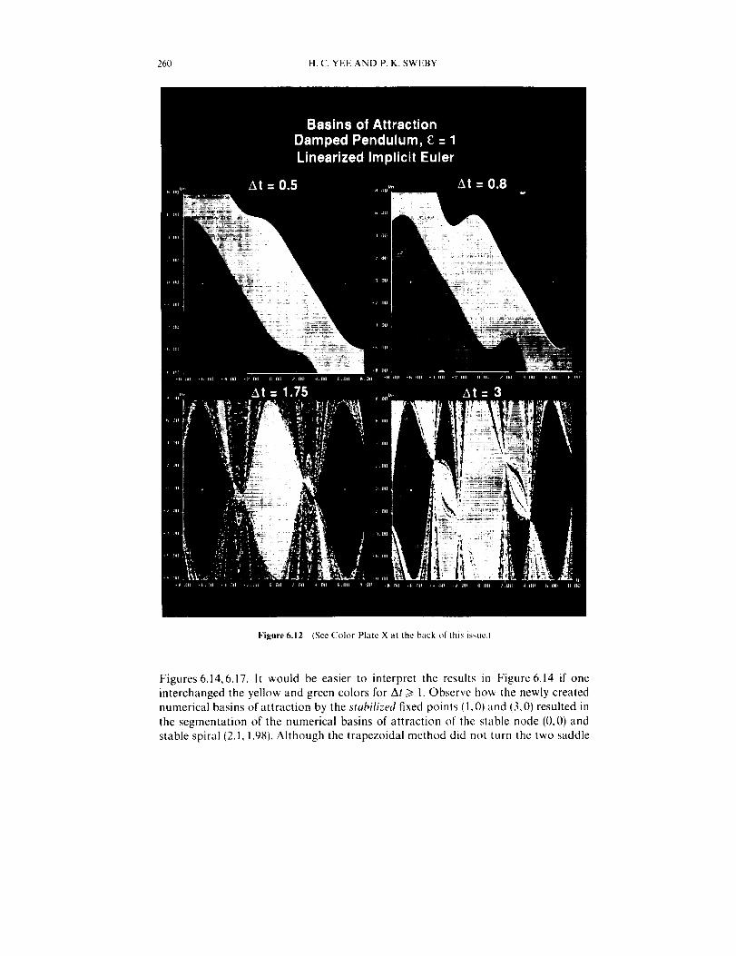
260 tt. C. YEE AND P. K. SWEBY
Figure 6.12 (SeeColor Plate X at the back of this issuc,]
Figures6.14,6.17. It would be easier to interpret the results in Figure6.14 if oneinterchanged the yellow and green colors for At _> 1. Observe how the newly created
numerical basins of attraction by the stabilized fixed points (t, 0) and (3, 0) resulted in
the segmentation of the numerical basins of attraction of the stable node (0,0) and
stable spiral (2.1, 1.98). Although the trapezoidal method did not turn the two saddle

I)YNAMICAI. STUDY O1. SPURIOUS STEADY-STATE NUMERICAl. SOLUTIONS 261
Figure 6.13 (See Color Plate XI al the back of this issue.}
points (1,0) and (3,01 into stable fixed points of different type, they did turn the two
saddle points into unstable fixed points of different type.
The evolution of the numerical basin of attraction as At changes is very traumatic
these implicit LM Ms. The cause of nonconvergence of these implicit LM Ms may due to
the fact that their numerical basins of attraction are fragmented. Take for example the

262 H.C. YEE AND P. K. SWEBY
,-?,
'-6
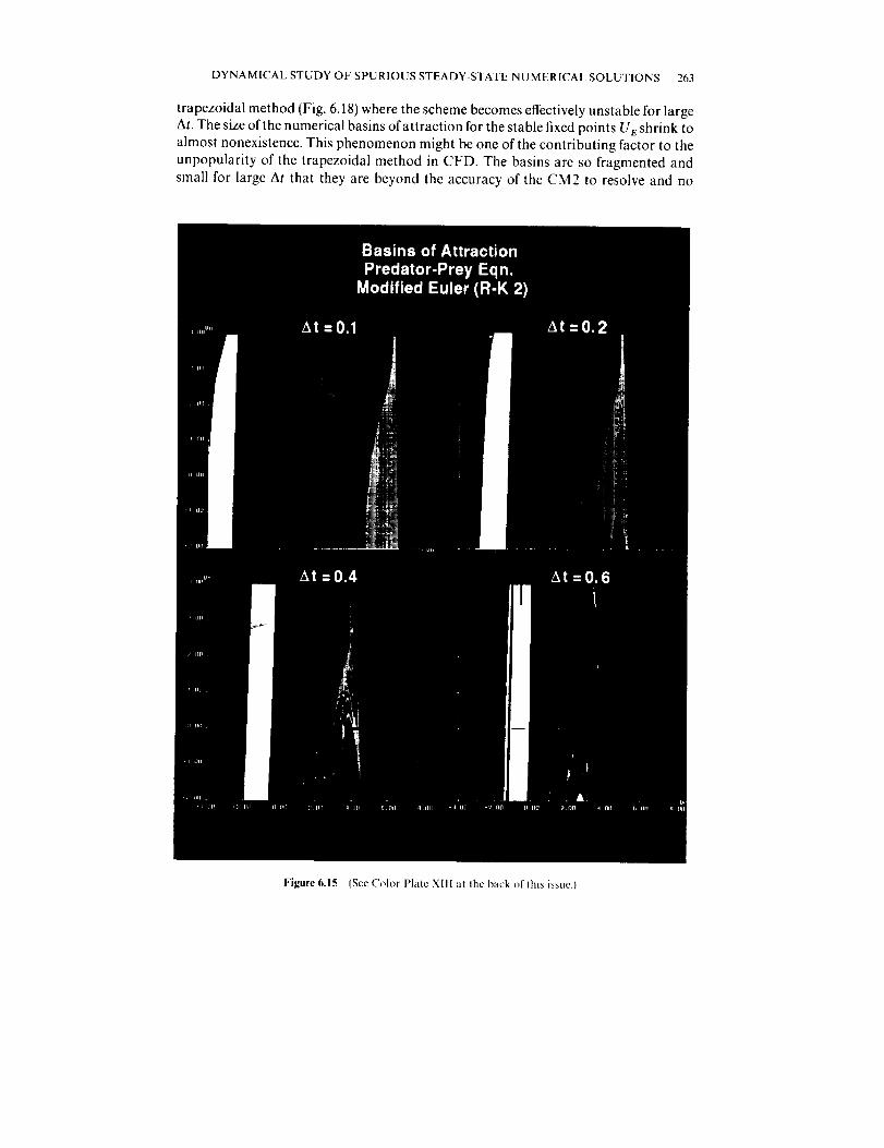
DYNAMICAL STUDY OF SPURIOUS STEADY-STATE NUMERICAL SOLUTIONS 263
trapezoidal method (Fig. 6.18) where the scheme becomes effectively unstable for largeAt. The size of the numerical basins of attraction for the stable fixed points U E shrink to
almost nonexistence. This phenomenon might be one of the contributing factor to the
unpopularity of the trapezoidal method in CFD. The basins are so fragmented and
small for large At that they are beyond the accuracy of the CM2 to resolve and no
Figure6.15 [SceColor Plate XIII at the back of this issue.)

264 H.C. YEE AND P. K. SWEBY
Figure 6.15 (Continued) (See Color Plate XIII at the back of this issue.)
further attempt was made. A better approach in computing these types of basins is touse interval arithmetic or the enclosure type method (Adams, 1990).
6.5 Numerical Resultsjor the Perturbed Hamiltonian Equation
Selected results for the two representations of numerical basins of attraction of the
various numerical methods for 4:= 0.1 are shown in Figures 6.19 6.25. Our studies

DYNAMICALSTUDYOFSPURIOUSSTF,ADY-STATENUMERICALSOLUTIONS265
Figure6.16 (See Color Plate XIV at the back of this issue.)
indicate that all of the studied Runge-Kutta methods exhibit spurious limit cycles andother spurious periodic solutions. For the Kutta and Heun methods, stable spurious
asymptotes can occur below the linearized stability limit of the scheme. The implicit
methods also exhibit spurious asymptotes. In particular, unstable spurious asymptoteswere produced below the linearized stability limit by all of the studied schemes.
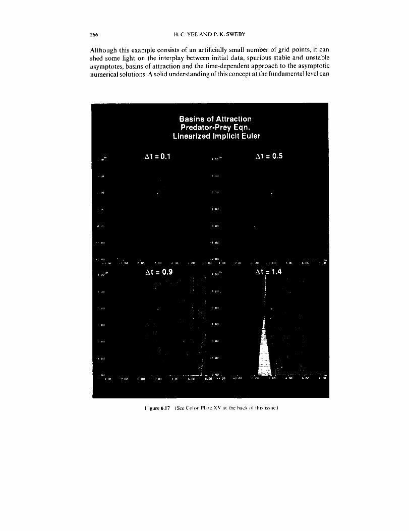
266 H.C.YEEANDP.K.SWEBY
Althoughthisexampleconsistsofanartificiallysmallnumberofgridpoints,it canshedsomelighton theinterplaybetweeninitialdata,spuriousstableandunstableasymptotes,basinsofattractionandthetime-dependentapproachto theasymptoticnumericalsolutions.Asolidunderstandingofthisconceptatthefundamentallevelcan
Figure6.17[SeeColorPlateXVatthebackofthisissuc.I
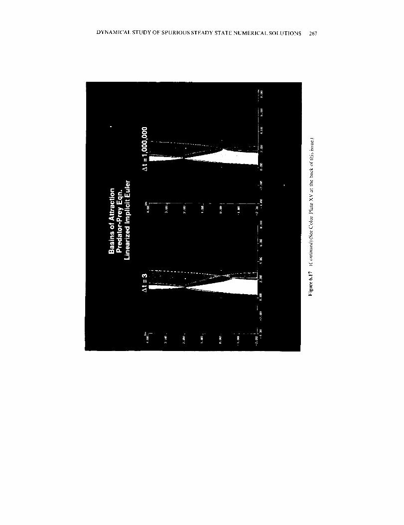
DYNAMICAL STUDY OF SPURIOUS STEADY-STATE NUMERICAL SOLUTIONS 267
2_
.g
03
"-6
v
k..,
m
,d
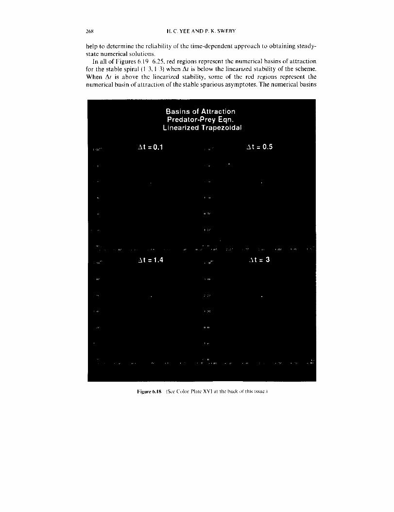
268 H.C. YEE AND P. K. SWEBY
help to determine the reliability of the time-dependent approach to obtaining steady-
state numerical solutions.
In all of Figures 6.19 6.25, red regions represent the numerical basins of attraction
for the stable spiral ( li3, t/3) when At is below the linearized stability of the scheme.
When At is above the linearized stability, some of the red regions represent the
numerical basin of attraction of the stable spurious asymptotes. The numerical basins
Figure 6.18 (See ('olor Plate XVI al the back of this issuc.I

DYNAMICAl. STUDY OF" SPURIOUS STEADY-STATE NUMERICAL SOLUTIONS 269
¢J
d=;
e.
,.-d
xca
"5
g
c._

270 H.C. YEE AND P. K. SWEBY
Figure 6.19 (See Color Plate XVII at the back of this issue.)
of attraction in Figures 6.21 with At = 0.1 appear to be the same as the exact basins of
attraction. Note also that the possibility of the numerical basin of attraction being
larger than the exact one does not always occur when the time step is the smallest. The
numerical basin of attraction for (1/3, 1/3) is larger than the corresponding exact basin
of attraction for At = I by the improved Euler and Kutta methods and for At = 0.1 by
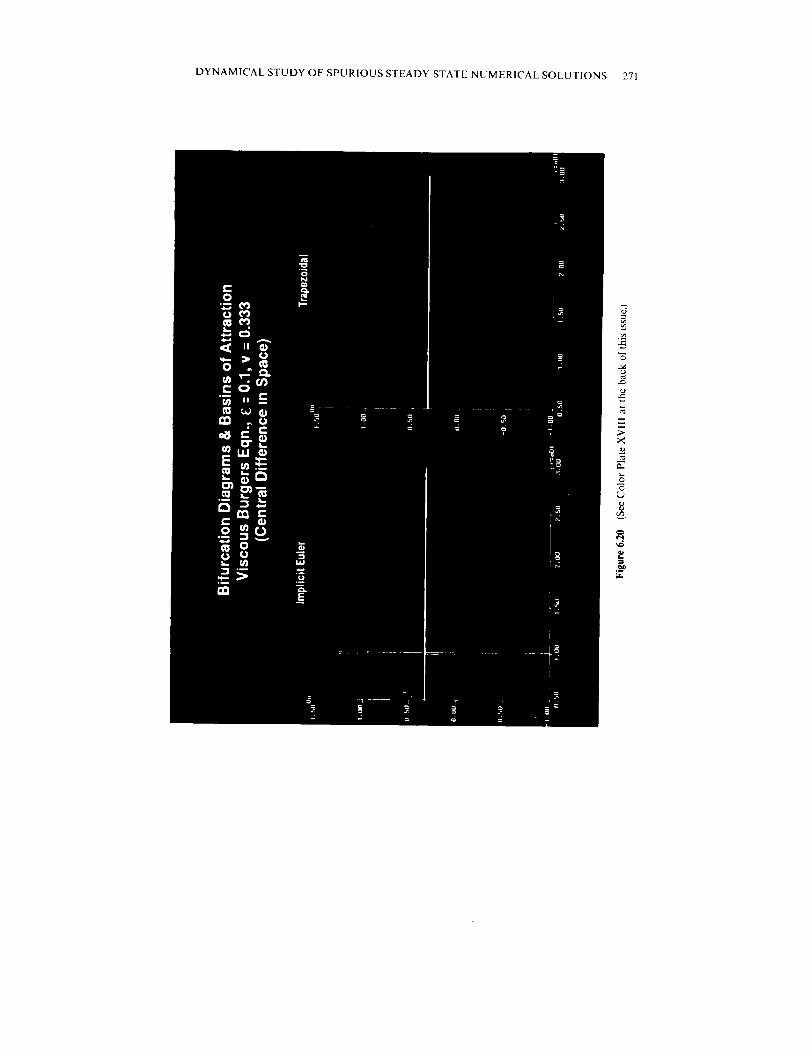
DYNAMICAL STUDY OF SPURIOUS STEADY-STATE NUMERICAL SOLUTIONS 271
A
.g
;>x
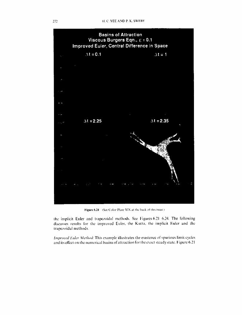
272 it.C.YEEANDP.K,SWEBY
Figure6.21(See Color I'lalc XIX at the back of this issue.)
the implicit Euler and trapezoidal methods. See Figures 6.21 6.24. The following
discusses results for the improved Euler, the Kutta, the implicit Euler and the
trapezoidal methods.
Improved Euler Method: This example illustrates the existence of spurious limit cycles
and its effect on the numerical basins of attraction for the exact steady state. Figure 6.21
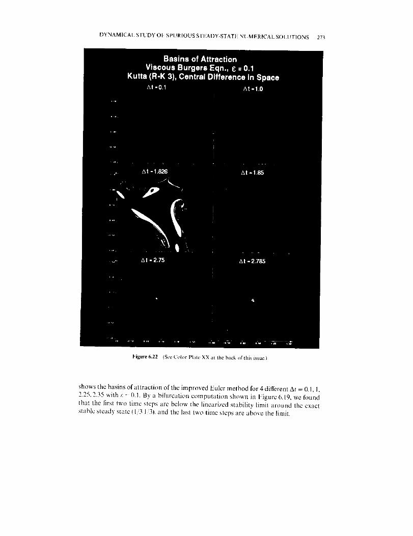
DYNAMICAL STUDY OF SPURIOUS STEADY-STATE NUMERICAL SOLUTIONS 273
Figure 6.22 [See Color Plate XX at the back of this issue,)
shows the basins of attraction of the improved Euler method for 4 different At = 0.1, 1,
2.25, 2.35 with _: = 0.1. By a bifllrcation computation shown in Figure 6.19, we found
that the first two time steps are below the linearized stability limit around the exact
stable steady state (I/3 1/31, and the last two time steps are above the limit.
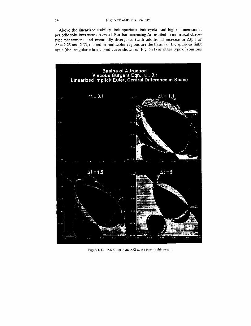
274 H.C. YEE AND P. K. SWEBY
Above the linearized stability limit spurious limit cycles and higher dimensional
periodic solutions were observed. Further increasing At resulted in numerical chaos-
type phenomena and eventually divergence (with additional increase in At). ForAt = 2.25 and 2.35, the red or multicolor regions are the basins of the spurious limit
cycle (the irregular white closed curve shown on Fig. 6.21) or other type of spurious
Figure 6.23 {See Color Plate XXl at the back of this issuc.I

DYNAMICALSTUDYOFSPURIOUSSTEADY-STATENUMERICALSOLUTIONS275
,,5
.¢=
x_
k_

276 H.C.YEEANDP.K.SWEBY
Figure6.24(SeeColorPlateXXII at the back of this issue.)
asymptote (white dots for Fig. 6.21). For these two time sleps the numerical basins for
the exact steady state (1/3, 1/3) by the improved Euler method disappeared. However, if
the initial data are in the red or multicolor region, one gets spurious solution instead of
what the linearized stability predicts divergent solution.
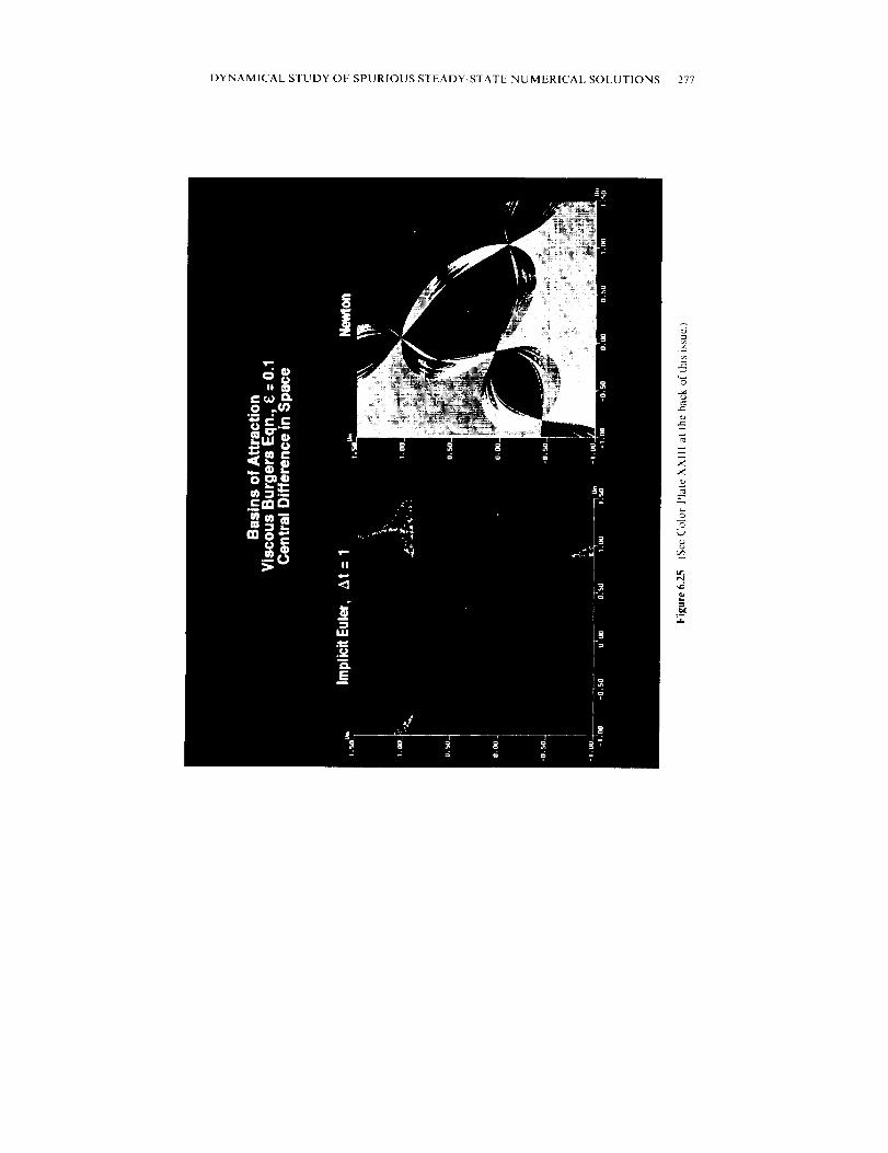
DYNAMICAL STUDY OF SPURIOUS STEADY-STATE NUMERICAL SOLUTIONS 277
A
,5
e-,
xx
oa
r,
©
(.,,
v
k_

278 H.C. YEE AND P. K. SWEBY
Kutta Method: To give an example of the existence of spurious stable asymptotes below
the linearized stability limit of the scheme, as well as the existence of spurious limit
cycles above the iinearized stability limit, Figure 6.22 shows the basins of attraction
of the Kutta method for 6 different fixed time steps At =0.l,l, 1.826,1.85,2.75 and2.785 (the first four below the linearized stability of the scheme) with e--0.1. For
At = 1.826, the numerical basin for (1/3, 1/3) has become fractal like with the birth of
fragmented, isolated new basins of attraction due to the presence of spurious periodic
solutions (the three white complicated closed curves with the associated purple, greenand blue basins shown in Fig. 6.22). The last two time steps in Figure 6.22 show the
diappearance of the numerical basin of attraction for the exact steady state with the
birth of basins for the spurious limit cycle.
Implicit Euler Method: This is yet another interesting illustration of the use of anunconditionally stable implicit method where in practical computations, when the
initial data are not known, the scheme has a higher chance of obtaining a physically
correct solution if one uses a At restriction slightly higher than that for the stability limit
of standard explicit methods (but with larger numerical basins of attraction than the
explicit method counterparts). Figures 6.20 and 6.23 show the two representations of
numerical basins of attraction using the implicit Euler method. These figures show the
generation of stable spurious asymptotes for At >/1. As At increases further, the size ofthe same numerical basin decreases and becomes fractal like, and new numerical basins
are generated. The behavior is similar to the predator-prey model (4.3) in a sense thatthe numerical basin of attraction for (1/3, 1/3) was permanently altered for At near or
larger than 10. Observe the fragmentation of the numerical basin of attraction for
(1/3, 1/3) by the basins of the spurious asymptotes.
Trapezoidal Method: Figures 6.20 and 6.24 show the two representations of numerical
basins of attraction using the trapezoidal method. As in the implicit Euler case, thisscheme has a higher probability of obtaining a physically correct solution if one uses a
At similar to that of standard explicit methods (but with larger numerical basins of
attraction than the explicit method counterparts). In a manner similar to the implicit
Euler, the numerical basins of attraction for (1/3, 1/3) are much larger than the
corresponding exact basin of attraction for At _<2. Their sizes are bigger than the ones
generated by the implicit Euler method with the same At values. The scheme becomes
effectively unstable due to the fragmentation of the numerical basins of attraction.
Again due to the high cost of double precision computations, no further attempts weremade for At large. The computation of these basins requires an interval arithmetic or
the enclosure-type (Adams, 1990) of mathematical operation before a more precisebehavior can be revealed.
Straight Newton t;s. Other Studied Methods: Figure 6.25 shows the basin of attraction
using Newton method in solving the steady part of the ODE (hereafter referred to as
straight Newton) compared with the implicit Euler at At = 1. One can see that straightNewton method has a smaller attracting basin for the stable spiral (1/3, 1/3) than the
implicit Euler method for small At. In fact its basin is the same as the implicit Euler
using larger At. Figure 6.25 illustrates the situation where quadratic convergence by theNewton method can be achieved only if the initial data are in the red regions.

DYNAMICAL STUDY OF SPURIOUS STEADY-STATE NUMERICAL SOLUTIONS 279
Figures 6.23 and 6.25 also illustrates the fact that using very large At by the (linearized)
implicit Euler method has the same chance of obtaining the correct steady state as theNewton method if the initial data are not known. Comparison of Newton method with
other iteration procedures for the implicit Euler and trapezoidal methods are reportedin our companion paper (Yee and Sweby, 1993a).
Combining the current result with Yee and Sweby (1993a), we can conclude that
contrary to popular belief, the initial data using the straight Newton method may nothave to be close to the exact solution for convergence. Straight Newton also exhibits
stable and unstable spurious asymptotes. Initial data can be reasonably removed fromthe asymptotic values and still be in the basin of attraction. However, the basins can be
fragmented even though the corresponding exact basins of attraction are single closed
domains. The cause of nonconvergence may just as readily be due to the fact that its
numerical basins of attraction are fragmented.
6.6 Global Asymptotic Behavior t_f lterative Implicit Schemes
The global asymptotic nonlinear behavior of some standard iterative procedures insolving nonlinear systems of algebraic equations arising from four implicit linear
multistep methods (LM Ms)in discretizing models (4.1), (4.3) and (4.4)is analyzed in our
companion paper (Yee and Sweby, 1993a). The implicit LMMs include implicit Euler,trapezoidal, mid-point implicit and three-point backward differentiation methods. The
iterative procedures include simple iteration and full and modified Newton iterations.
The results are compared with standard Runge-Kutta explicit methods, a non-iterative
implicit procedure, and straight Newton method. Here we give a summary of Yee and
Sweby (1993a) so that the reader may get a bigger picture of implicit methods otherthan the ones studied in this paper.
Studies in Yee and Sweby (1993a) showed that all of the four implicit LMMsexhibit a drastic distortion but less shrinkage of the basin of attraction of the true
solution than standard explicit methods studied in this paper. In some cases withsmaller At, the implicit LMMs exhibit enlargement of the basins of attraction of
the true solution. Overall, the numerical basins of attraction of a non-iterative im-
plicit procedure mimic more closely the basins of attraction of the continuum than
the studied iterative implicit procedures for the four implicit LMMs. In general thenumerical basins of attraction bear no resemblance to the exact basins of attraction.
The size can increase or decrease depending on the time step. Also the possible existenceof the largest numerical basin of attraction that is larger than the exact one does
not occur when the time step is the smallest. The dynamics of numerics of the implicit
methods differ significantly from each other, and the different methods of solvingthe resulting non-linear algebraic equations are very different from each other
since different numerical methods and solution procedures result in entirely differentnonlinear discrete maps. Although unconditionally stable implicit methods allow
a theoretically large time step At, the numerical basins of attraction (allowable initial
data) for large At some-times are so fragmented and/or so small that the safe (or
practical) choice of At is slightly larger or comparable to the stability limit of standard
explicit methods (but with larger numerical basins of attraction than the explicit
method counterparts). In general, ifone uses a At that is a fraction of the stability limit,

280 H.C.YEEANDP.K.SWEBY
onehasahigherchanceofconvergenceto thecorrectasymptotethanthestandardexplicitmethods.
Studiesin YeeandSweby(1993a)alsoshowedthatthevariabletimestepcontrolmethodcanoccasionallystabilizeunstablefixedpoints,dependingontheinitialdata,startingtimestepandtheiterativetolerancevalue.OneshortcomingisthatthesizeofAtneededtoavoidspuriousdynamicsisimpracticalto use,especiallyfortheexplicitmethod.
7. CONCLUDINGREMARKS
TheglobalasymptoticnonlinearbehaviorandbifurcationphenomenafortheexplicitEulermethod,fivedifferentmultistageRunge-Kuttamethods(modifiedEuler,improvedEuler,Heun,Kuttaand4th-ordermethods),twoandthree-steppredictor-correctormethods,Adams-Bashforthmethod,andimplicitEulerandtrapezoidalmethodwithlinearizationarecomparedfordifferentmodelnonlinearODEs.ThefivemultistageRunge-Kuttamethodsandthepredictor-correctormethodsarenonlinearin thediscretizedparameterspaceAtandall LMMsarelinearin At.Withtheaidof theCM-2,thecomplexbehaviorandsometimesfractallikestructureof theassociatednumericalbasinsofattractionofthesetimediscretizationsarecomparedandrevealedforthefirsttime.
ThenumericalresultsindicatethatwithsufficientlysmallAtandinitialdataclosetothesteadystate(usuallynotknownforthetime-marchingmethod),onecanhavethehighestchanceofconvergencetothecorrectasymptote.Ingeneral,theinitialdatacanbefarremovedfromtheexactsteadystatebythestudiedimplicitmethodsprovidedthatafractionoftheallowabletimesteprestrictionisused.Ourstudyalsoindicatesthatbifurcationto aperiodtwoor lowerorderperiodsolutonisreadilydetectableinnumericalcalculations.However,bifurcationto a limitcyclewillnotbesoobvioustwithoutaphaseportraitrepresentation),especiallyin thevicinityofthebifurcationpoint.Indeedthephenomenonofanartificialtimeiterationtosteady-stateofalargesystemformedbyspatialdiscretizationwhichnearsconvergencebeforetheresiduals"plateausout",couldactuallybetheresultofastablespuriouslimitcyclearoundtheHopfbifurcationpoint.Inaddition,thebifurcationofspiralstolimitcyclesmightaccountinpartforthephenomenonofnear(butlackof)convergencein largestiffsystems.
ForagiveninitialdataandtwofinitebutdifferentAt'sthatarebelowthelinearizedstabilitylimitofthescheme,theirnumericalsolutionsmightconvergetotwodifferentsolutionsevenifnospuriousstable steady-state numerical solution is introduced by thescheme and the initial data are physically relevant. The source of the behavior is due to
the existence of unstable spurious asymptotes or stable asymptotes other than steady
states which have the same detrimental tin terms of robustness_ effect. However, in the
case of occurrence of stable spurious steady states, they can be mistaken for the true
steady state in practical computations. In other words depending on the initial data, for
a given At below the linearized stability limit, the numerical solution can (a) converge
to the correct steady state, Ib) converge to a different steady state, (ct converge to
a spurious periodic solution, (d) yield spurious asymptotes other than (a_ Icl, or ie)
diverge, even though the initial data are physically relevant.
DYNAMICAL STUDY OF SPURIOUS STEADY-STATE NUMERICAL SOLUTIONS 281
Another important finding is that unlike the scalar first-order autonomous ODEdiscussed in part I (Yee et al., 1991), the fixed points can change types as the time step is
varied even for two-time-level unconditionally stable implicit LMMs. An unstable
fixed point can become a stable fixed point and can e.g., change from a saddle to a stable
or unstable node (for a fixed system parameter t:). Since these implicit methods can
introduce spurious asymptotes as well, thus even though LM Ms preserve the same
number but not the same types of fixed points as the underlying DEs, the numerical
basins ofattraction of LM Ms (explicit or implicit l do not always coincide with the exact
basins of attraction of the underlying DEs. One major consequence of this behavior isthat the flow pattern can change type as the discretized parameter is varied. Another
consequence of these phenomena is the fragmentation of the numerical basin of attrac-
tion. In general, unconditionally stable implicit LMMs exhibit less shrinkage of the
basin of attraction of the true solution than standard explicit methods. Another
interesting result is that contrary to popular belief, the initial data using the straight
Newton method may not have to be close to the exact steady state for convergence.
However, we believe that one cause of nonconvergence in straight Newton or implicitLM Ms with large time step may due to the fact that the numerical basins of attraction
are fragmented.
in conclusion, the present results can explain some of the roots of why one cannot
achieve the theoretical linearized stability limit of the typical implicit Euler andtrapezoidal time discretization in practice when solving strongly nonlinear DEs, e.g. in
CFD. The results can also shed some light in bridging some of the gaps between
theoretical convergence criterion (At---, 0, as n--* ,:f_)and practical scientific computa-
tion (finite At as n -_ _c:).
Ackmm'led_lements
The authors wish to thank A. M. Stuart and D. F. Griffiths for their valuable discussions during the course of
this research and for suggesting the model equations 14.1 ) and 14.4}. Special thanks to A. Lafon, M.Vinokur,
T. Coakley and C. Y. McNeil for their critical review oflhe manuscript. Financial support from T. Lasinski
for the second author as a visiting scientist at NASA Ames is greatfully acknowledged.
Adams, E. ( 19901 '" Periodic Solutions: Enclosure, Verilication, and Applications", Computer Arithmetic and
Se!12Validating Numerical Methods, Academic Press, 199 245.
Beam, R. M. and Bailey, H, E. (19881 "Direct Solver for Navier-Stokes Equations", Proceedings of Interna-
tional Conference on Computational Engineering Science, Atlanta, GA.
Beam, R. M. and Warming, R. F. (1976)"An Implicit Finite-Difference Algorithm for Hyperbolic Systems in
Conservation Law Form", J. Comput. Phv.s,, 22, 87 110.Budd, C. J., Stuart, A. M., Koomullil, G. P. and Yee, H. C. (1994) "Numerical Solution Behavior of Model
(['onvection-Diffusion BVP with Grid Adaptation", in preparation.
Foias. C., Sell, G. and Temam, R. ( 1985)"Varietes Iner tielles des Equations Differentielles Dissipati'¢es", C.R.
Acad. Sci. Paris, Ser. 1 Math., 301,139 141.
Globus, A., Levit, C. and Lasinski, T. (1991) "A Tool for Visualizing the Topology of Three-Dimensional
Vector Fields", NAS Applied Research Branch Report RNR-91-017, NASA Ames Research Center.
Gri_fitbs, D. F., Sweby, P. K. and Yee, It. C. 11992a) "On Spurious Asymplotes Numerical Solutions of
Explicit Runge-Kuna Schemes", IMA J. Nurner. Anal,, 12, 319 338.
Grift]ths, D. F., Stuart, A. M. and Yee, H. C. ( 1992b)"Numerical Wave Propagation in Hyperbolic Problemswith Nonlinear Source Terms", SIAM J. of'Numer. Anal)'., 29(5), 1244 1260.
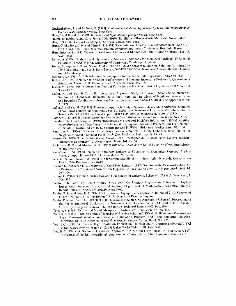
282 H.C.YEE AND P. K. SWEBY
Guckenheimer, J. and Holmes, P. (1983) Nonlinear Oscillations, Dynamical Systems, and Bifurcations of
Vector Fields, Springer-Verlag, New York.Hale, J. and K ocak, H. (I 991) Dynamics and BiJurcations, Springer-Verlag, New York.Hairer, E., lserles, A. and Sanz-Serna, J. M. (1989) "Equilibria of Runge-Kutta Methods", Namer. Math.
Hsu, C. S. (19871 CeU-to-Cell Mappin.q, Springer-Verlag, New York.
Hung, C. M., Sung, C. H and Chen, C. L. (1991) "Computation o1_Saddle Point of Attachment", AIAA-91-1713, AIAA 22nd Fluid Dynamics, Plasma Dynamics and Lasers Conference Honolulu, Hawaii.
Humphries, A. R. (19921 "'Spurious Solutions of Numerical Methods for Initial Value problems", IMA J.Num. ,4 nal.
Iserles, A. 11988_ "Stability and Dynamics of Numerical Methods for Nonlinear Ordinary Differential
Equations", DAMTP NA I, University of Cambridge, Cambridge, England.Iserles, A., Pcplow, A. T. and Stuart, A, M. (1990) "A Unified Approach to Spurious Solutions Introduced by
Time Discretisation". Part 1: Basic Theory, DAMTP 1990 NA4 Numerical Analysis Reports, Univer-
sity of Cambridge.Jameson, A. (1991)"'Airfoils Admitting Nonunique Solutions to the Euler Equations", AIAA-91-1625.
Keller, |t. B. 11977t"Numerical Solution of Bifurcation and Nonliner Eigenvalue Problems", Applications o!
Bi[urcation Theory. P. tt. Rabinowitz, ed.. Academic Press, 359 384.Kwak, M. 11991) "Finite l)imensional Inertial Forms for the 3D Navier-Stokcs Equations," IMA preprinl
Series #828.
Lafon, A. and Yee, HC. {1991)"'Dynamical Approach Study of Spurious Steady-State Numerical
Solutions for Nonlinear Differential Equations", Part 111: The Ettects of Nonlinear Source Terms
and Boundary Conditions in Reaction-Convection Equations, NASA TM-103877, to appear in Intern.J. CFD.
Lafon, A. and Yee, H, C, 119921 "'Dynamical Approach Study of Spurious Steady-State Numerical Solutionsof Nonlinear l)ifferential Equations", Part IV: Stability vs. Numerical Treatment of Nonlinear Source
Terms, ONERA-CERT Technical Report DERAT 4550115.38. to appear in Intern. J. CFD.
Lambert, J. D, I 973) Computational Methods in Ordinary Dilh'rential Equations, John Wiely, Ne_' York,
Langford, W. F, and looss, G. (198(I)"Interactions of Hopf and Pitchfork Bifurcations", ISNM 54, Bi/ur-cation Problems and Their Numerical Solution, Workshop on Bifurcation Problems and Their Numeri-
cal Solution, Dortmund, ed. H. D. Mittelmann and It, Weber, Birkhauser Verlag, Basel, 103 134.
Panov. A. M. (19561 "Behavior of the Trajectories of a System of I:inite Difference Equations in thc
Neighbourhood of a Singular Point", Uch. Zap. Urt._l. Gos. Unit. rvp, 19, 89 99.Perron, O. 11929} "'Ubcr Stabilitat and Asymtotisches Uberhalten de I,i_sungen eines Systems endlicher
Differenzengleichungen", J. Reine An,qew. Math., 161, 41 64.
Richtmyer, R. D, and Morton, K. W. 119671 Di_lbrence Methods liar hmm/-lrah,, Problems, lnterscience-
Wiely, New York,Sanz-Serna. J, M. 1199111 "'Numerical Ordinary l)ifferential Equations l)ynamical Systems," Applied
Math ('omput. Report 1990, 3, Universidad de Valladolid,Schectcr, S. and Shearer, M. 1199(11 "'Undercompressive Shocks for Nonstrictl) Ityperbolic Conservation
Laws", IMA Preprinl Series #619.Shearer, M., Schaeffer. 11. G., Marchesin, D. and Paes-Leme, P. 119871 "S_lution of the Riemann Problem fl)r
a Prototype 2 × 2 S)stem of Non-Strictly ltyperbolic ('onscrvalion Laws", Arch. Rat. Mech. Anal., 97.299 320.
Strang, G. (19681 "On the ('onstruction and Comparison of Diflizrcncc Schemes", SIAM J. Num. Anal., 5,506 517.
Sweby, P. K.. Ycc. H ('. and Grifliths, D. F. (19901 "On Spurious Steady-State Solutions of Explicit
Runge-Kutta Schemes", I.lniversity of Reading, Department of Mathematics, Numerical Analysis
Report 390, also NASA TM 102819, April 1990.Sweby, P. K. and Yec. tt C. 119911 "'On Spurious Asymptotic Numerical Solutions of 2 × 2 Systems of
ODEs". Numerical analysis Report 7,,,'91, University of Reading, England.
Sweby, P. K. and Ycc, tt. C 119941 "On the Dynamics of Somc Grid Adaptation Schemes", Proceedings ofthe 4th International ('onlY:fence on Numerical Grid Generation in Ct'D and Related Fields,"
University ('ollegc of Swansea, U K, also RIACS TEchnical Report 94.02. Feb. 1994.Temam, R. 11989_ "Do Inertial Manifolds Apply to Turbulence'?", I'hvsica D, 37, 146 152.
Warner, B. (19801 "Turning Points of Branches of Positive Solutions", ISNM 54. Bili_rcation Problems and
Their Numerical Solution, Workshop on Bifurcation Problems and Their Numerical Solution,Dortmund, ed. H. D. Mitlelmann and H. Weber, Birkhauser Verlag, Basel, 211 226.
Yee H.C. (19891 "A ('lass of High-Resolution Explicit and hnplicit Shock-('apturing Methods", VKI
Lecture Series 1989 04 March 6 10, 1989, also NASA TM-101088. I"eb. 1989.
Yee, H. C. (1991i "A Nonlinear Dynamical Approach to Algorithm I)evelopmcnt in ltypersonic CFD',
Proccedings of the 4th International symposium on Computational I'luid Dynamics, Davis, Calif.
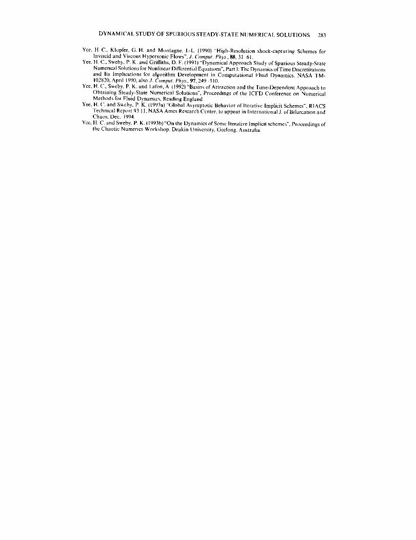
DYNAMICALSTUDYOFSPURIOUSSTEADY-STATENUMERICALSOLUTIONS283
Yee,H.C.,Klopfer,G.H.andMontagne, J.-L. (1990) "High-Resolution shock-capturing Schemes forInviscid and Viscous Hypersonic Flows", d. Comput. Phys., 88, 31 61.
Yee, H. C., Sweby, P. K. and Gritfiths, D. F. (I 991)"Dynamical Approach Study of Spurious Steady-StateNumerical Solutions for Nonlinear Differential Equations", Part 1:The Dynamics of Time Discretizations
and Its Implications for algorithm Development in Computational Fluid Dynamics, NASA TM-102820, April 1990, also d. Cornput. Phys., 97, 249 310.
Yee, H. C., Sweby, P. K. and Lafon, A. (1992)"Basins of Attraction and the Time-Dependent Approach toObtaining Steady-State Numerical Solutions", Proceedings of the 1CFD Conference on Numerical
Methods for Fluid Dynamics, Reading England.
Yee, H. C. and Sweby, P. K. (1993a) "Global Asymptotic Behavior of lterative Implicit Schemes", RIACSTechnical Report 93.11, NASA Ames Research Center, to appear in International J. of Bifurcation andChaos, Dec., 1994.
Yee, H. C. and Sweby, P. K. (1993b)"'On the Dynamics of Some lterative Implicit schemes", Proceedings ofthe Chaotic Numerics Workshop, Deakin University, Geelong, Australia.

Color Plate I Figure 6.1 (See H.C. Yee and P. K. Sweby.)
Color Plate II Figure 6.2 (See H.C. Yee and P. K. Sweby.)

Color Plate III Figure 6.3 (See H.C. Yec and P. K. Swcby.)

ColorPlateIV Figure6.4(SeeH.C. Yee and P. K. Sweby.)

r-
_P
cj
cs_
_oo_
0

Color Plate VI Figure 6.8 (See H.C. Yee and P. K. Sweby.)
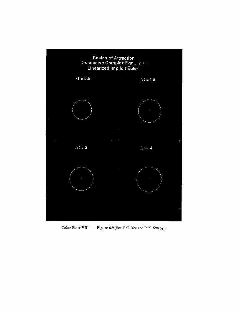
Color Plate VII Figure 6.9 (See H.C. Yee and P. K. Sweby.)

Color Plate VIII Figure 6.10 (See H.C. Yee and P. K. Sweby.)

oli
114
0
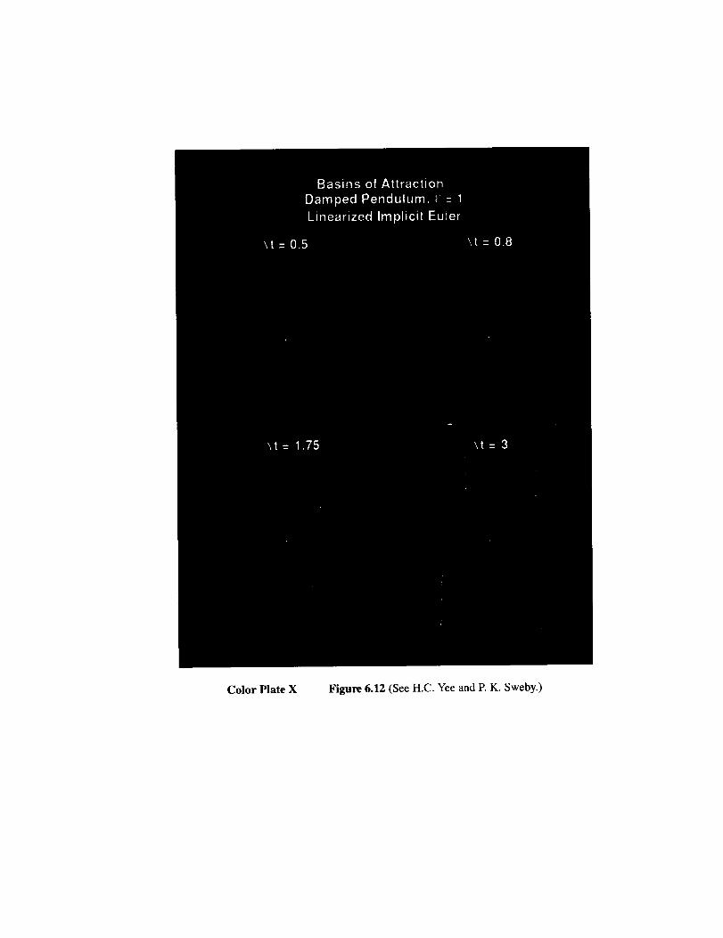
Color Plate X Figure 6.12 (See H.C. Yee and R K. Sweby.)

Color Plate XI Figure 6.13 (See H.C. Yee and P. K. Sweby.)
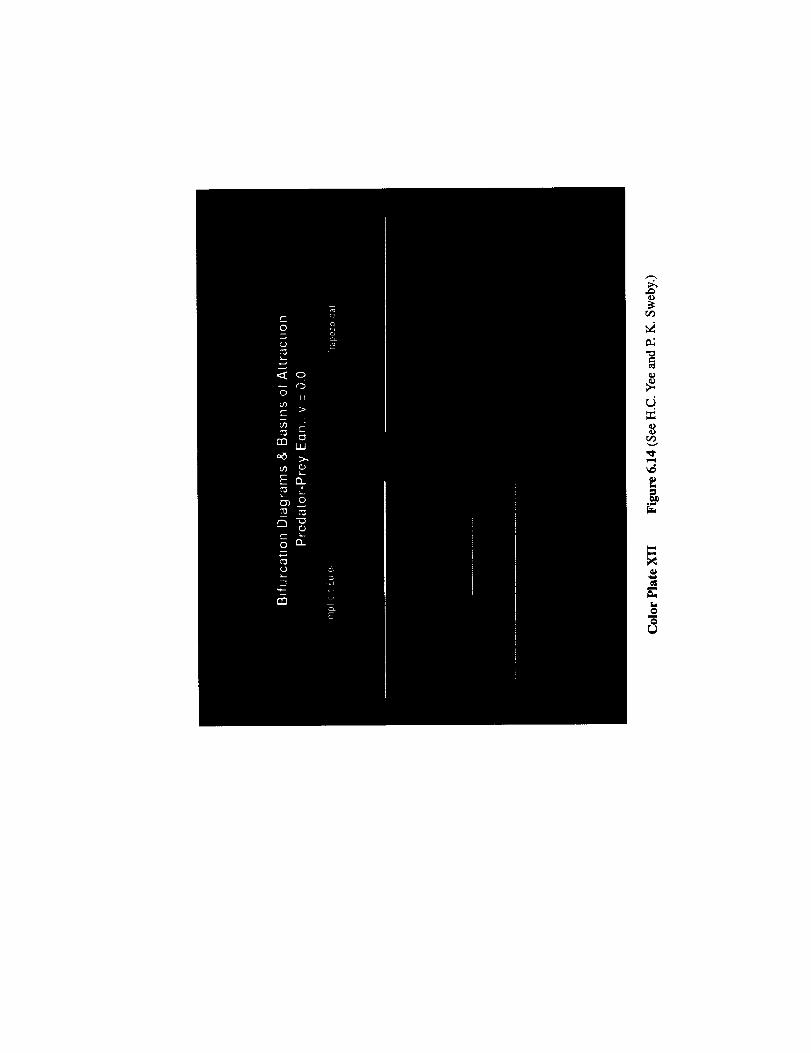
_s
_J
_P
v
rut
r_
_S
0
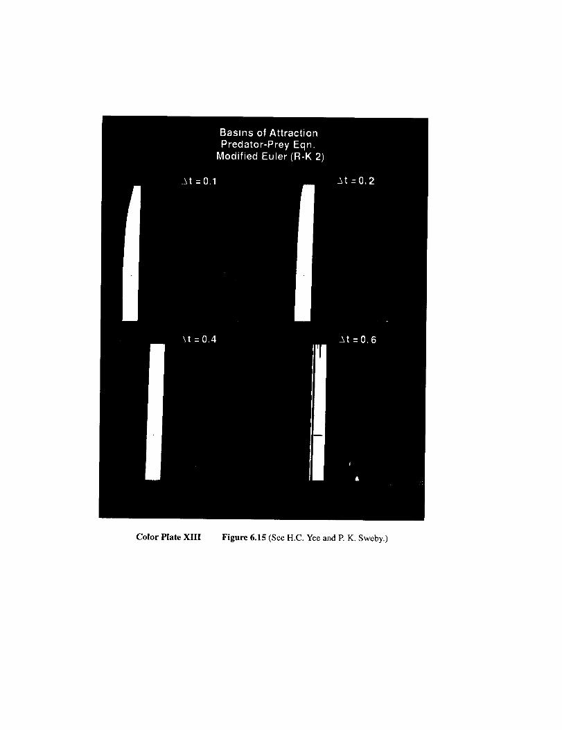
Color Plate XIII Figure 6.15 (See H.C. Yee and R K. Sweby.)
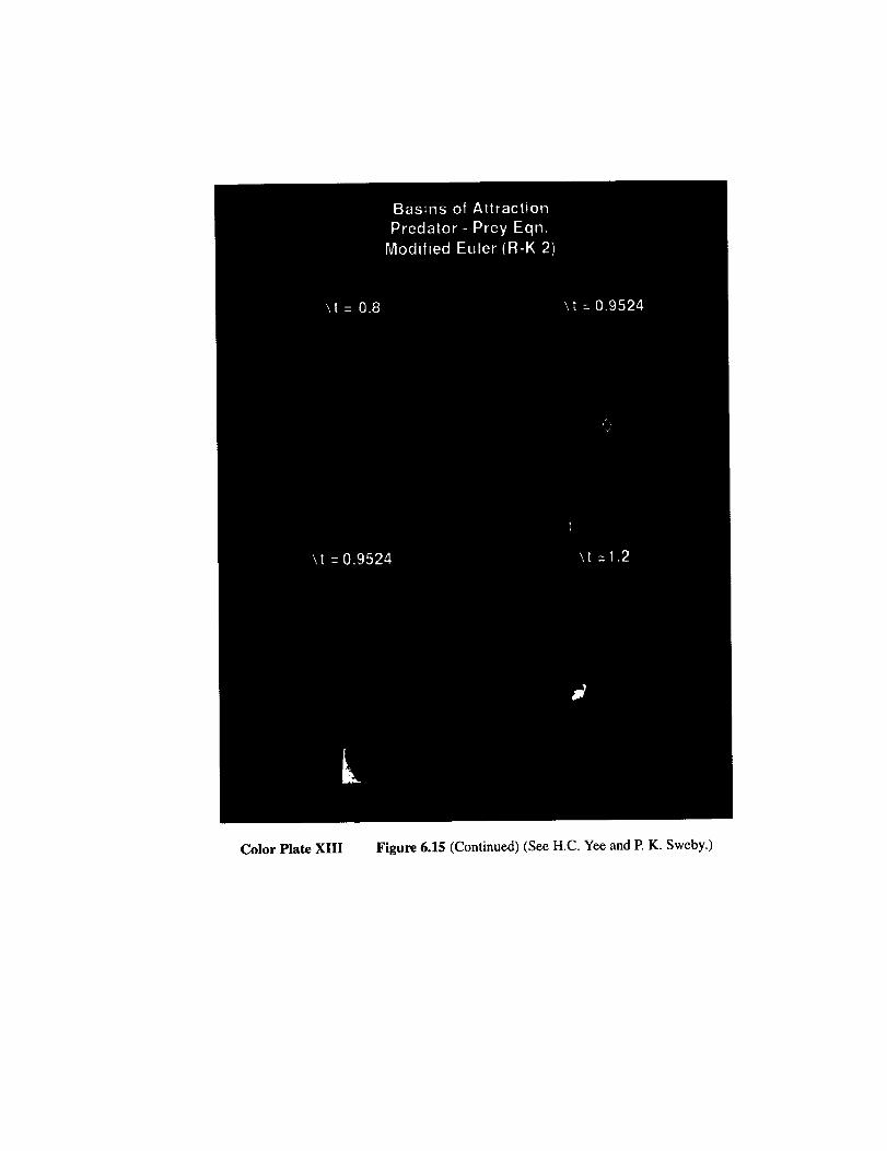
Color Plate XIlI Figure 6.15 (Continued) (See H.C. Yee and P. K. Sweby.)

ColorPlate XIV Figure 6.16 (See H.C. Yee and E K. Sweby.)

Color Plate XV Figure 6.17 (See H.C. Yee and P. K. Sweby.)

n_
oo
0

Color Plate XVI Figure 6.18 (See H.C. Yee and P. K. Sweby.)
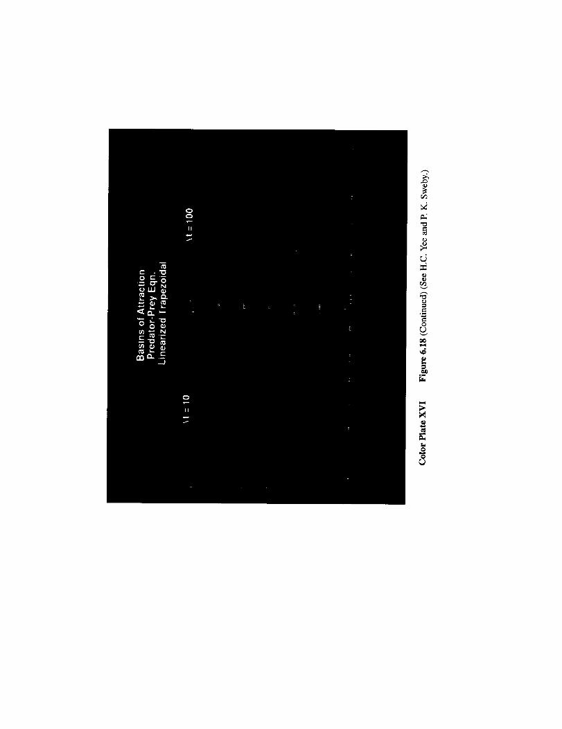
_J
0
fuC_

Color Plate XVII Figure 6.19 (See H.C. Yee and P. K. Sweby.)

CS_
c_
_J
_0°Jr
L
0
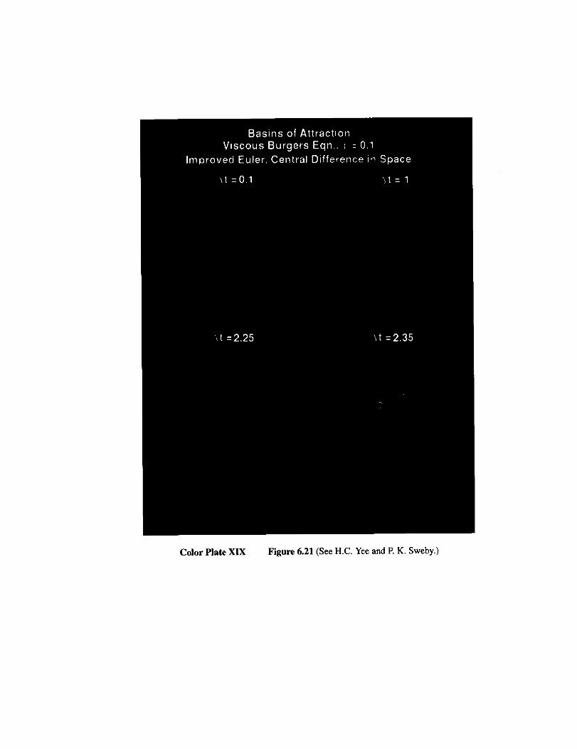
Color Plate XIX Figure 6.21 (See H.C. Yee and P. K. Sweby.)
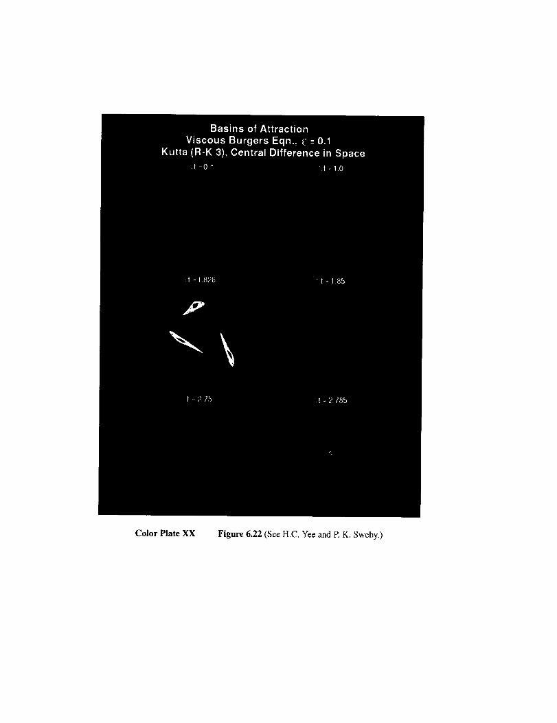
ColorPlateXX Figure6.22(See H.C. Yee and P. K. Sweby.)

Color Plate XXI Figure 6.23 (See H.C. Yee and P. K. Sweby.)

_J
q_
0
_J
C_
I.i0
0
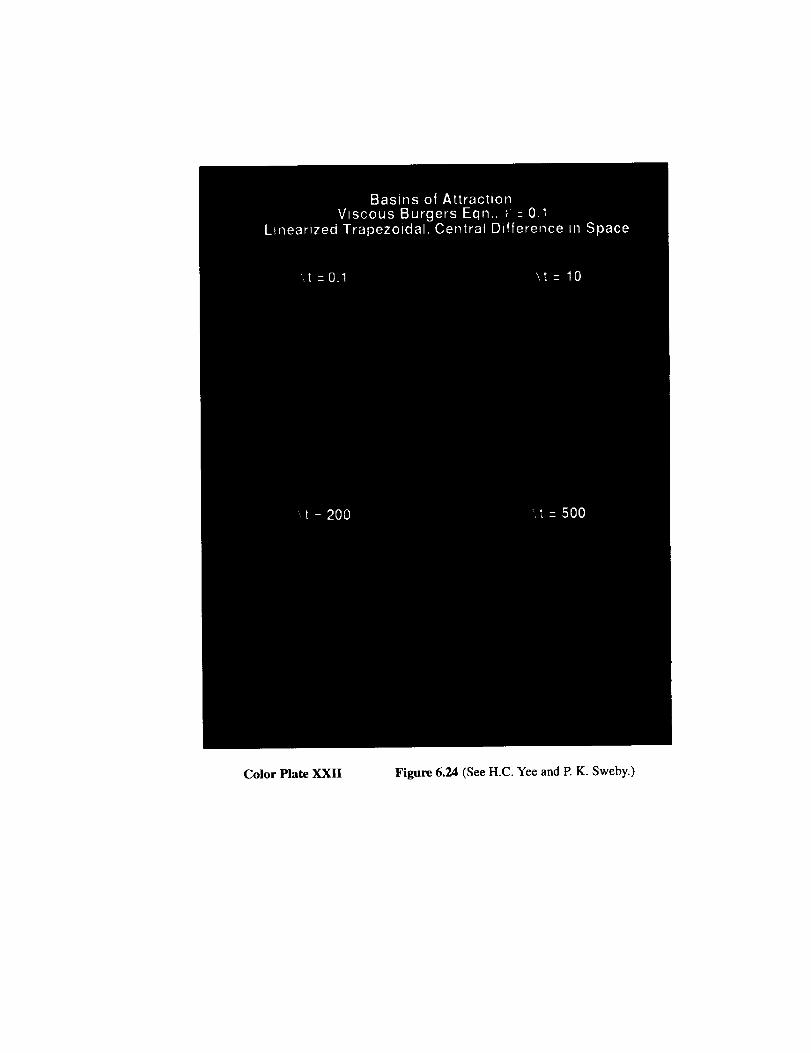
Color Plate XXII Figure 6.24 (See H.C. Yee and P. K. Sweby.)
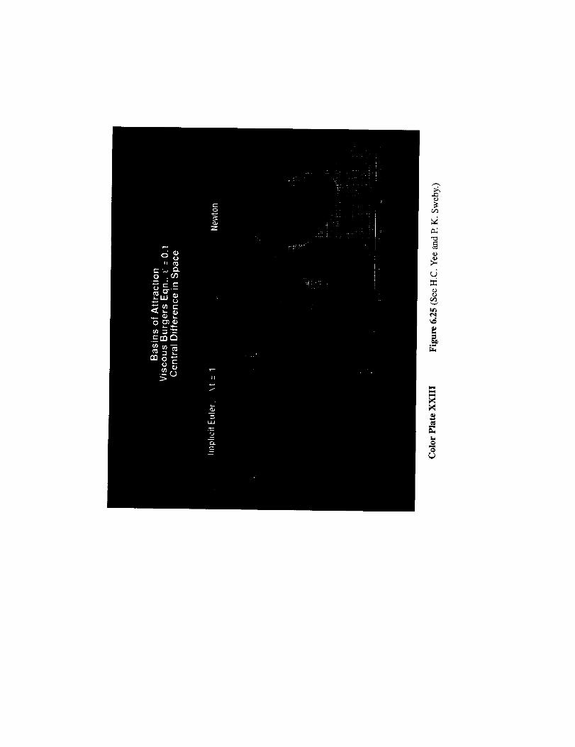
_3
c__P
_J
Lf_
m_
L0
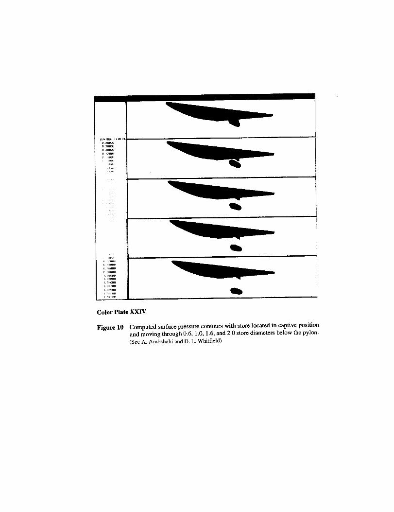
I:[IN 1111141I I Ul I
O. _6Ol]l[l
D. 7o0O0
[).:|rmoo
ii.:_']lillll
_l,_, _,
• F_rlii
:+
: tl_]i
ii ,l:,lllJl+
l]._I llJUU
++. <ll,llU|i
U. '+IJLIUILI
I,UtlUOII
I,l_;'nlrlll
I •11,1nnfl
I flnllO[I
I 1o11011
I I ;'flflfl
Color Plate XXIV
Figure 10 Computed surface pressure contours with store located in captive positionand moving through 0.6, 1.0, 1.6, and 2.0 store diameters below the pylon.(See A. Arabshahi and D. L. Whitfield)