Dynamic Trading Strategies in the Presence of Market Frictions
156
Dynamic Trading Strategies in the Presence of Market Frictions Mehmet Sa˘ glam Submitted in partial fulfillment of the requirements for the degree of Doctor of Philosophy under the Executive Committee of the Graduate School of Arts and Sciencess COLUMBIA UNIVERSITY 2012
Transcript of Dynamic Trading Strategies in the Presence of Market Frictions
Dynamic Trading Strategies in the Presence of MarketFrictions
Mehmet Saglam
Submitted in partial fulfillment of the
requirements for the degree of
Doctor of Philosophy
under the Executive Committee
of the Graduate School of Arts and Sciencess
COLUMBIA UNIVERSITY
2012

© 2012
Mehmet Saglam
All Rights Reserved
ABSTRACT
Dynamic Trading Strategies in the Presence of MarketFrictions
Mehmet Saglam
This thesis studies the impact of various fundamental frictions in the microstructure of fi-
nancial markets. Specific market frictions we consider are latency in high-frequency trading,
transaction costs arising from price impact or commissions, unhedgeable inventory risks due
to stochastic volatility and time-varying liquidity costs. We explore the implications of each
of these frictions in rigorous theoretical models from an investor’s point of view and derive
analytical expressions or efficient computational procedures for dynamic strategies. Spe-
cific methodologies in computing these policies include stochastic control theory, dynamic
programming and tools from applied probability and stochastic processes.
In the first chapter, we describe a theoretical model for the quantitative valuation of
latency and its impact on the optimal dynamic trading strategy. Our model measures the
trading frictions created by the presence of latency, by considering the optimal execution
problem of a representative investor. Via a dynamic programming analysis, our model
provides a closed-form expression for the cost of latency in terms of well-known parameters
of the underlying asset. We implement our model by estimating the latency cost incurred by
trading on a human time scale. Examining NYSE common stocks from 1995 to 2005 shows
that median latency cost across our sample more than tripled during this time period.
In the second chapter, we provide a highly tractable dynamic trading policy for portfolio
choice problems with return predictability and transaction costs. Our rebalancing rule is
a linear function of the return predicting factors and can be utilized in a wide spectrum
of portfolio choice models with minimal assumptions. Linear rebalancing rules enable to
compute exact and efficient formulations of portfolio choice models with linear constraints,
proportional and nonlinear transaction costs, and quadratic utility function on the terminal

wealth. We illustrate the implementation of the best linear rebalancing rule in the context
of portfolio execution with positivity constraints in the presence of short-term predictability.
We show that there exists a considerable performance gain in using linear rebalancing rules
compared to static policies with shrinking horizon or a dynamic policy implied by the
solution of the dynamic program without the constraints.
Finally, in the last chapter, we propose a factor-based model that incorporates common
factor shocks for the security returns. Under these realistic factor dynamics, we solve
for the dynamic trading policy in the class of linear policies analytically. Our model can
accommodate stochastic volatility and liquidity costs as a function of factor exposures.
Calibrating our model with empirical data, we show that our trading policy achieves superior
performance in the presence of common factor shocks.
Table of Contents
1 Introduction 1
1.1 The Cost of Latency . . . . . . . . . . . . . . . . . . . . . . . . . . . . . . . 2
1.2 Linear Rebalancing Rules . . . . . . . . . . . . . . . . . . . . . . . . . . . . 4
1.3 Common Factor Shocks in Strategic Asset Allocation . . . . . . . . . . . . . 5
1.4 Organization of the Thesis . . . . . . . . . . . . . . . . . . . . . . . . . . . . 6
2 The Cost of Latency 8
2.1 Introduction . . . . . . . . . . . . . . . . . . . . . . . . . . . . . . . . . . . . 8
2.1.1 Related Literature . . . . . . . . . . . . . . . . . . . . . . . . . . . . 14
2.2 A Stylized Execution Model without Latency . . . . . . . . . . . . . . . . . 16
2.2.1 Limit Order Execution . . . . . . . . . . . . . . . . . . . . . . . . . . 17
2.2.2 Optimal Solution . . . . . . . . . . . . . . . . . . . . . . . . . . . . . 19
2.3 A Model for Latency . . . . . . . . . . . . . . . . . . . . . . . . . . . . . . . 22
2.4 Analysis . . . . . . . . . . . . . . . . . . . . . . . . . . . . . . . . . . . . . . 25
2.4.1 Dynamic Programming Decomposition . . . . . . . . . . . . . . . . . 25
2.4.2 Asymptotic Analysis . . . . . . . . . . . . . . . . . . . . . . . . . . . 29
2.4.3 Discreteness of Time vs. Latency . . . . . . . . . . . . . . . . . . . . 31
2.4.4 Extensions . . . . . . . . . . . . . . . . . . . . . . . . . . . . . . . . 33
2.5 Empirical Estimation of Latency Cost . . . . . . . . . . . . . . . . . . . . . 34
2.5.1 The Optimal Policy and the Approximation Quality . . . . . . . . . 35
2.5.2 Historical Evolution of Latency Cost . . . . . . . . . . . . . . . . . . 39
2.5.3 Historical Evolution of Implied Latency . . . . . . . . . . . . . . . . 42
i
2.5.4 Empirical Importance of Latency . . . . . . . . . . . . . . . . . . . . 42
2.6 Conclusion and Future Directions . . . . . . . . . . . . . . . . . . . . . . . . 44
3 Linear Rebalancing Rules 47
3.1 Introduction . . . . . . . . . . . . . . . . . . . . . . . . . . . . . . . . . . . . 47
3.1.1 Related Literature . . . . . . . . . . . . . . . . . . . . . . . . . . . . 51
3.2 Dynamic Portfolio Choice with Return Predictability and Transaction Costs 54
3.2.1 Examples . . . . . . . . . . . . . . . . . . . . . . . . . . . . . . . . . 56
3.3 Optimal Linear Model . . . . . . . . . . . . . . . . . . . . . . . . . . . . . . 61
3.4 Efficient Exact Formulations . . . . . . . . . . . . . . . . . . . . . . . . . . . 67
3.4.1 Linear Constraints . . . . . . . . . . . . . . . . . . . . . . . . . . . . 68
3.4.2 Transaction Costs . . . . . . . . . . . . . . . . . . . . . . . . . . . . 70
3.4.3 Terminal Wealth and Risk Aversion . . . . . . . . . . . . . . . . . . 71
3.5 Application: Equity Agency Trading . . . . . . . . . . . . . . . . . . . . . . 73
3.5.1 Formulation . . . . . . . . . . . . . . . . . . . . . . . . . . . . . . . . 75
3.5.2 Approximate Policies . . . . . . . . . . . . . . . . . . . . . . . . . . . 76
3.5.3 Upper Bounds . . . . . . . . . . . . . . . . . . . . . . . . . . . . . . 79
3.5.4 Model Calibration . . . . . . . . . . . . . . . . . . . . . . . . . . . . 80
3.5.5 Numerical Results . . . . . . . . . . . . . . . . . . . . . . . . . . . . 82
3.6 Conclusion . . . . . . . . . . . . . . . . . . . . . . . . . . . . . . . . . . . . 83
4 Common Factor Shocks 86
4.1 Introduction . . . . . . . . . . . . . . . . . . . . . . . . . . . . . . . . . . . . 86
4.1.1 Related literature . . . . . . . . . . . . . . . . . . . . . . . . . . . . . 87
4.2 Model . . . . . . . . . . . . . . . . . . . . . . . . . . . . . . . . . . . . . . . 88
4.2.1 Security and factor dynamics . . . . . . . . . . . . . . . . . . . . . . 88
4.2.2 Cash and stock position dynamics . . . . . . . . . . . . . . . . . . . 90
4.2.3 Objective function . . . . . . . . . . . . . . . . . . . . . . . . . . . . 90
4.2.4 Linear policies . . . . . . . . . . . . . . . . . . . . . . . . . . . . . . 92
4.2.5 Closed form solution . . . . . . . . . . . . . . . . . . . . . . . . . . . 95
4.3 Experiment . . . . . . . . . . . . . . . . . . . . . . . . . . . . . . . . . . . . 97
ii
4.3.1 Characteristics versus Factor-based return generating model . . . . . 97
4.3.2 Calibration of main parameters . . . . . . . . . . . . . . . . . . . . . 98
4.3.3 Approximate policies . . . . . . . . . . . . . . . . . . . . . . . . . . . 100
4.3.4 Simulation Results . . . . . . . . . . . . . . . . . . . . . . . . . . . . 103
4.4 Conclusion and Future Directions . . . . . . . . . . . . . . . . . . . . . . . . 104
Bibliography 104
A The Cost of Latency 114
A.1 Dynamic Programming Decomposition . . . . . . . . . . . . . . . . . . . . . 114
A.2 Proof of Theorem 2 . . . . . . . . . . . . . . . . . . . . . . . . . . . . . . . . 119
A.3 Proof of Theorem 3 . . . . . . . . . . . . . . . . . . . . . . . . . . . . . . . . 126
A.4 Price Dynamics with Jumps . . . . . . . . . . . . . . . . . . . . . . . . . . . 132
B Linear Rebalancing Rules 137
B.1 Proof of Lemma 3 . . . . . . . . . . . . . . . . . . . . . . . . . . . . . . . . 137
B.2 Exact Formulation of the Terminal Wealth Objective . . . . . . . . . . . . . 138
B.3 Derivation of the LQC Policies . . . . . . . . . . . . . . . . . . . . . . . . . 140
B.4 Exact Formulation of Best Linear Execution Policy . . . . . . . . . . . . . . 141
iii
List of Figures
2.1 An illustration of the limit order execution in the stylized model. . . . . . . 19
2.2 An illustration of an optimal strategy with no latency. . . . . . . . . . . . . 21
2.3 An illustration of the model of latency. . . . . . . . . . . . . . . . . . . . . . 23
2.4 An illustration of the optimal policy of Theorem 2. . . . . . . . . . . . . . . 28
2.5 An illustration of the optimal strategy for GS, expressed in terms of limit
price premium over the course of the time, for different choices of latency. . 37
2.6 An illustration for the evolution of the continuation value of the optimal
policy over time for GS, for different choices of latency. . . . . . . . . . . . 38
2.7 An illustration of the latency cost as a function of the latency. . . . . . . . 38
2.8 An illustration of the historical evolution of latency cost over the 1995–2005
time period. . . . . . . . . . . . . . . . . . . . . . . . . . . . . . . . . . . . . 41
2.9 An illustration of the historical evolution of implied latency over the 1995–
2005 time period. . . . . . . . . . . . . . . . . . . . . . . . . . . . . . . . . . 43
iv

List of Tables
3.1 Summary of the performance statistics of each policy, along with upper bounds. 84
3.2 Detailed comparison between the alpha gains, transaction costs, and total
performance of the optimal linear policy and projected dynamic policy. . . . 85
4.1 Calibration results for λ and Ω. . . . . . . . . . . . . . . . . . . . . . . . . 99
4.2 Summary of the performance statistics of each policy in the case of no com-
mon factor noise and low transaction cost environment. . . . . . . . . . . . 103
4.3 Summary of the performance statistics of each policy in the case of no com-
mon factor noise and high transaction cost environment. . . . . . . . . . . . 104
4.4 Summary of the performance statistics of each policy in the case of common
factor noise and low transaction cost environment. . . . . . . . . . . . . . . 105
4.5 Summary of the performance statistics of each policy in the case of common
factor noise and high transaction cost environment. . . . . . . . . . . . . . . 105
v

AcknowledgmentsThe research in this thesis resulted from collaborations with my advisor Professor Cia-
mac C. Moallemi and my committee members Professor Collin-Dufresne and Professor Kent
Daniel. While my long meetings with each of them have taught me a lot in theory and
methodological tools, I am specifically indebted to their friendship and continuous support
in establishing my academic training.
I would like to particularly thank Professor Ciamac Moallemi, who served as my aca-
demic advisor during my entire time at Columbia and provided constructive feedback for all
my academic endeavors – from a standard homework question to an hour-long conference
presentation. His professional attitude along with his sincere mentorship in all life matters
is an exemplary figure that I will try to imitate in the rest of my career.
I am deeply grateful to my committee member Professor Pierre Collin-Dufresne, who
taught me everything I know about dynamic asset pricing and continuous-time finance.
From him, I learned the significance of building insights around mathematical formulas and
the virtue of judgmental analysis without falling into the deception of number crunching.
I am further indebted to my committee members Professor Mark Broadie and Professor
Paul Glasserman for reading my thesis carefully and their valuable suggestions and advice.
I would like to especially thank my classmates and friends from Columbia with whom my
tenure as a student in New York was very enjoyable. I would like to specifically acknowledge
Santiago Balseiro, Burak Baskurt, Soner Bilge, Berk Birand, Deniz Çiçek, Ezgi Demirdag,
Cem Dilmegani, Caner Göçmen, Neset Güner, Damla Günes, Çınar Kılçıoglu, Serdar Ko-
caman, Paulita Pontiliano, Ahmet Serdar Simsek, Erinç Tokluoglu, Cengiz Üçbenli, and
Izzet Yıldız.
I am very thankful to my wife, Merve Sehiraltı Saglam, for her tremendous support, con-
tinuous patience and unlimited love that turned the difficult and stressful days of graduate
vi

life into the most happiest and unforgettable.
Finally, I would like to thank my family, Nagihan Saglam, Yusuf Saglam, Ilknur Saglam
Altun, Ümit Saglam and Ibrahim Altun for their invaluable support and unconditional love.
I would like to specifically thank my parents for their utmost dedication and unbounded
sacrifice that helped me reach this success. This thesis is dedicated to my family.
vii

To my family
viii
CHAPTER 1. INTRODUCTION 1
Chapter 1
Introduction
Classical finance models are based on an assumption of frictionless markets in one-period
horizon. This simplicity usually provides ease in obtaining tractable models. However, it
is not usually clear whether the one-period solution will have similar properties with the
dynamic solution in the multi-period setting. Multi-period objective differs significantly
from single-period objective by incorporating the ability to have decision with recourse
which better reflects the actual objective of many investors in highly uncertain financial
markets.
Incorporating financial frictions into the model is certainly a step forward to the “true”
model of financial markets. Recent research that incorporates these frictions has shown us
that these frictions may explain various anomalies observed in financial markets such as
sudden liquidity dry-ups, the pricing of hard-to-borrow stocks, and valuation in over-the-
counter markets.
Aiming to address these two perspectives, this thesis studies how various market frictions
influence the investor’s optimal decisions dynamically when underlying states of the econ-
omy are stochastic. Specific market frictions I have considered are latency in high-frequency
trading, common and hidden factors in equity returns, transaction costs in portfolio rebal-
ancing, unhedgeable inventory and residual risks due to stochastic volatility. I explored
the implications of each of these frictions in rigorous theoretical models from an investor’s
point of view and derived analytical expressions or efficient computational procedures for
dynamic strategies. Specific methodologies in computing these policies include stochastic

CHAPTER 1. INTRODUCTION 2
control theory, dynamic programming and tools from applied probability and stochastic
processes.
This thesis theoretically concerns with optimal (or near-optimal) dynamic decision mak-
ing in high-dimensional stochastic systems. My motivating research problems in this setting
have originated from financial markets, yet, they are intrinsically operational questions:
the impact of technological improvement in your trading system on your profit, the opti-
mal control of transaction costs while trading with return predicting signals, and utilizing
approximate trading rules when there are complex interactions between expected future
returns and volatility and liquidity.
This thesis provides insightful contributions by enhancing our understanding of the
implications of these frictions and suggests easy-to-implement strategies. In a nutshell, I
believe that my research can help
• quantify the explicit cost of latency in high frequency trading and shed light on the
very timely impact of speed in trading microstructure.
• characterize a near-optimal strategy to exploit return predictability while controlling
transaction costs,
• propose a closed-form approximate policy for strategic asset allocation when returns
exhibit factor driven covariance structure.
With these common distinguishing features, each chapter of my dissertation can be
studied further in detail. In each chapter, the impact of the friction on the dynamic trading
strategy is extensively studied, the dynamic problem is clearly posed and an optimal or
near-optimal dynamic decision rule is derived.
1.1. The Cost of Latency
A very recent friction quoted extensively in the popular media has been latency, the delay
between a trading decision and the resulting trade execution. As high frequency trading
has flourished and subsequent regulatory questions about this trading activity have become
a central focus of interest, thanks in part to the acclaimed “Flash Crash” on May 6th, 2010,
CHAPTER 1. INTRODUCTION 3
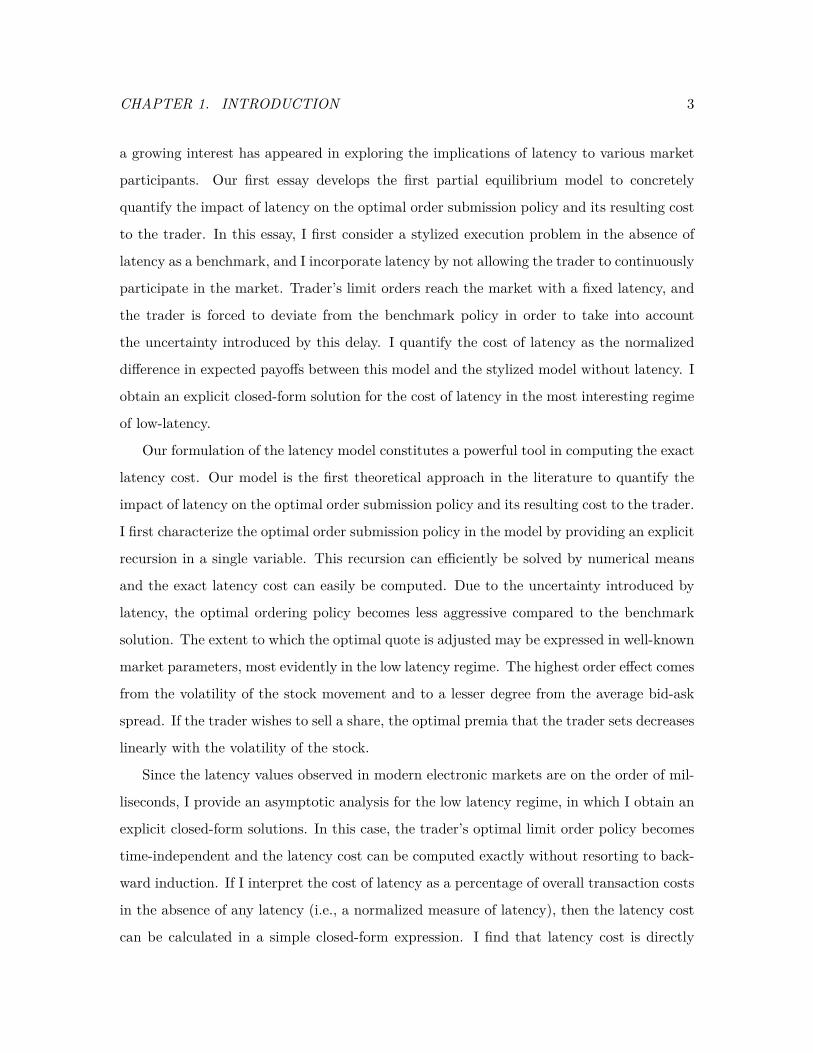
a growing interest has appeared in exploring the implications of latency to various market
participants. Our first essay develops the first partial equilibrium model to concretely
quantify the impact of latency on the optimal order submission policy and its resulting cost
to the trader. In this essay, I first consider a stylized execution problem in the absence of
latency as a benchmark, and I incorporate latency by not allowing the trader to continuously
participate in the market. Trader’s limit orders reach the market with a fixed latency, and
the trader is forced to deviate from the benchmark policy in order to take into account
the uncertainty introduced by this delay. I quantify the cost of latency as the normalized
difference in expected payoffs between this model and the stylized model without latency. I
obtain an explicit closed-form solution for the cost of latency in the most interesting regime
of low-latency.
Our formulation of the latency model constitutes a powerful tool in computing the exact
latency cost. Our model is the first theoretical approach in the literature to quantify the
impact of latency on the optimal order submission policy and its resulting cost to the trader.
I first characterize the optimal order submission policy in the model by providing an explicit
recursion in a single variable. This recursion can efficiently be solved by numerical means
and the exact latency cost can easily be computed. Due to the uncertainty introduced by
latency, the optimal ordering policy becomes less aggressive compared to the benchmark
solution. The extent to which the optimal quote is adjusted may be expressed in well-known
market parameters, most evidently in the low latency regime. The highest order effect comes
from the volatility of the stock movement and to a lesser degree from the average bid-ask
spread. If the trader wishes to sell a share, the optimal premia that the trader sets decreases
linearly with the volatility of the stock.
Since the latency values observed in modern electronic markets are on the order of mil-
liseconds, I provide an asymptotic analysis for the low latency regime, in which I obtain an
explicit closed-form solutions. In this case, the trader’s optimal limit order policy becomes
time-independent and the latency cost can be computed exactly without resorting to back-
ward induction. If I interpret the cost of latency as a percentage of overall transaction costs
in the absence of any latency (i.e., a normalized measure of latency), then the latency cost
can be calculated in a simple closed-form expression. I find that latency cost is directly
CHAPTER 1. INTRODUCTION 4
proportional to the ratio of volatility and the average bid-ask spread. Thus, latency cost
increases for more volatile or less liquid stocks. The dependence on the observed latency,
is more complex with the first order contribution coming from the variance of the stock
price during the latency interval and a second order adjustment that will enable to secure
execution in the asymptotic limit. In order to derive this cost empirically, I only need
to estimate the volatility, the average bid-ask spread of the stock and the intrinsic value
of latency. This is an elegant and practical result as the estimation procedures for these
quantities are readily abundant in the literature.
1.2. Linear Rebalancing Rules
One of the most well-studied market frictions is the impact of transaction costs on the
optimal portfolio choice of the investor. Furthermore, when the investor has predictions for
the expected future returns using return predicting factors such as market capitalization,
book-to-market ratio, lagged returns, dividend yields, determining an optimal dynamic
policy with realistic risk and trading constraints is almost certainly intractable.
Faced with this daunting task, this essay provides a highly tractable rebalancing rule for
dynamic portfolio choice problems with return predictability and transaction costs. This
rebalancing rule is a linear function of return predicting factors and can be utilized in a
wide spectrum of portfolio choice models with realistic considerations for risk measures,
transaction costs and constraints. As long as the starting dynamic portfolio optimization
problem is a convex programming problem, the modified optimization problem seeking the
optimal parameters of the linear decision rule will be a convex programming problem.
I provide a large class of dynamic portfolio choice models that differ in their modeling
of risk measures, transaction costs and constraints which can be formulated as determin-
istic convex optimization problems. Specifically, I compute the analytic expression of the
objective function in the cases with quadratic utility function on the terminal wealth or
proportional and nonlinear transaction cost functions. Finally, I derive efficient formula-
tions for incorporating linear equality and inequality constraints. If there does not exist an
analytic expression for the objective, the optimal parameters can be solved via the sampling
CHAPTER 1. INTRODUCTION 5
techniques available from the sample average and stochastic approximation literature.
Finally, I implement the computation of the best linear policy in the context of portfolio
execution, the execution of a large long position in a single security. For this purpose, I
need positivity constraints on portfolio positions and the amount of shares sold in each
period in order to achieve a feasible execution. In order to compare the performance of
the best linear rebalancing rule, I use the identical discrete-time setup of Garleanu and
Pedersen [2012] for which a closed-form solution is available in the lack of constraints. I
calibrate the model parameters using two-days of transactions data on a liquid stock and
construct two predictors in a high-frequency setting with different mean reversion speeds.
The simulation implemented with these predictors and calibrated parameters reveal that
the best linear policy performs better than the deterministic policy, model predictive control
and a projected version of the optimal policy proposed by Garleanu and Pedersen [2012].
1.3. Common Factor Shocks in Strategic Asset Allocation
The foundations developed in the second chapter have been influential in analyzing the
impact of common factor shocks when there are transaction costs and return predictability.
In this essay, I take a deeper look at a particular dynamic portfolio choice problem with
common factor shocks driving security returns. I propose a new factor model for security
returns in which each security has its own return predicting factors based on short-term
reversal, momentum, and long term reversal. In this model, I correctly account for the
conditional variance of returns by allowing co-movements with factor exposures. I utilize
linear decision rules in past returns and factor exposures for our dynamic trading strategy.
I show that the optimal linear policy can be computed in closed-form in contrast to recent
parametric approaches that rely on numerical optimization.
Garleanu and Pedersen [2012] has been a break-through by combining trading frictions
with return predictability in a highly tractable model that actually allowed closed-form so-
lution. However, this tractability has emerged with an obvious cost, a significant departure
from standard dynamic portfolio choice literature. The simplifying assumption has been
using number of shares in the portfolio decision vector in order to linearize the state dy-
CHAPTER 1. INTRODUCTION 6
namics. Using number of shares versus dollar holdings also required to model price changes
in dollars instead of percentage terms. This is clearly problematic as it allows for negative
prices. Furthermore, it is well-known that price changes are not stationary, cannot be es-
timated effectively using linear regression techniques. In this essay, I keep the nonlinear
structure in the wealth evolution but instead of trying to solve the problem to optimality, I
use linear policies in order to obtain a near-optimal policy. I obtain a closed-form solution
for our policy parameters which allows us to expand the universe of parameters quite easily.
I evaluate the performance of our linear policy in a well-calibrated simulation. Our
simulation study shows that best linear policy provides significant benefits compared to
other approximate policies recently studied in the literature, especially when the transac-
tion costs are high and returns evolve according to factor dependent covariance structure.
Unlike other parametric approaches, our modeling provides a closed form solution instead
of statistical fitting procedure. Analytical tractability allows us to expand our universe of
parameters which allows for greater flexibility in obtaining different policy rules for different
asset classes.
1.4. Organization of the Thesis
The balance of this thesis is organized as follows:
Chapter 2 provides a formal model to quantify the cost of latency. I present a stylized,
continuous-time trade execution problem in the absence of latency. I develop a variation
of the model with latency and provide a mathematical analysis of the optimal policy for
our problem. By contrasting the results in the presence and absence of latency, I am able
to quantitatively assess the cost of latency. In a later section, I consider some empirical
applications of the model.
Chapter 3 presents the abstract form of a dynamic portfolio choice model and provide vari-
ous specific problems that satisfy the assumptions of the abstract model. I formally describe
the class of linear decision rules and discuss solution techniques in order to find the optimal
parameters of the linear policy. I provide efficient and exact formulations of dynamic port-
folio choice models using linear decision rules. In this generalized approach, I incorporate
CHAPTER 1. INTRODUCTION 7
linear equality and inequality constraints, proportional and nonlinear transaction costs and
a measure of terminal wealth risk. Finally, I apply our methodology in an optimal execution
problem and evaluate the performance of the best linear policy.
Chapter 4 provides a methodology that can address complex return predictability models in
multi-period settings with transaction costs. Our return predicting factors does not need to
follow any pre-specified model but instead can have arbitrary dynamics. I allow for factor
dependent covariance structure in returns driven by common factor shocks and illustrate in
a simulation study that linear policies perform very well in these intractable models.
CHAPTER 2. THE COST OF LATENCY 8
Chapter 2
The Cost of Latency
2.1. Introduction
In the past decade, electronic markets have become pervasive. Technological advances in
these markets have led to dramatic improvements in latency, or, the delay between a trading
decision and the resulting trade execution. In the past 30 years, the time scale over which
a trade is processed has gone from minutes1
One factor behind this trend has been competition between exchanges, as one mechanism
for differentiation between exchanges is latency. This competition is driven by a significant
demand amongst a class of investors, sometimes called “high frequency” traders, for low
latency trade execution. High frequency traders are thought to account for more than half
of all US equity trades.3 They expend significant resources in order to develop algorithms
and systems that are able to trade quickly. For example, on the time scale of milliseconds,
the speed of light can become a binding constraint on the delay in communications. Hence,
traders seeking low latency will “co-locate”, or house their computers in the same facility as
the exchange, in order eliminate delays due to a lack of physical proximity. This co-location1NYSE, pre-1980 upgrade [Easley et al., 2008]. to milliseconds2 — “low latency” in a contemporary
electronic market would be qualified as under 10 milliseconds, “ultra low latency” as under 1 millisecond.
This change represents a dramatic reduction by five orders of magnitude. To put this in perspective, human
reaction time is thought to be in the hundreds of milliseconds.3“Stock traders find speed pays, in milliseconds,” New York Times, July 23, 2009.

CHAPTER 2. THE COST OF LATENCY 9
comes at a significant expense, however it has been stated that a 1 millisecond advantage
can be worth $100 million to a major brokerage firm.4
There has been much discussion of the importance of latency among various market
participants, regulators, and academics. Despite the significant amount of recent interest,
however, latency remains poorly understood from a theoretical perspective. For example,
how does latency relate to transaction costs? Is latency only relevant to investors with
short time horizons, such as high frequency traders, or does latency also affect long term
investors such as pension funds and mutual funds? Many of these important questions have
been considered in anecdotal or ad hoc discussions. My goal here is to provide a framework
for quantitative analysis of these issues.
In particular, I wish to understand the benefit to a single trader in the marketplace
of lowering their latency, while holding everything else fixed. This is a different question
than understanding the social costs of latency, i.e., whether in equilibrium the collective
marketplace is better or worse off given lower latency. One might imagine, for example, that
the benefit to a individual agents of lower latency may diminish in an equilibrium setting.
Equilibrium or welfare analysis of low latency trading is a complex question with important
policy and regulatory implications. I believe that understanding the single-agent effects
of low latency trading, however, is an important first step which will inform my ultimate
understanding of collective effects.
The cost that a trader bears due to latency can take many different forms, depending
on the precise trading strategy. However, a number of broad themes can be identified,5
sometimes overlapping, as to why the ability to trade with low latency might be valuable
to an investor:
1. Contemporaneous decision making. A trader with significant latency will be
making trading decisions based on information that is stale.
For example, consider an automated trader implementing a market-making strategy
in an electronic limit order book. The trader will maintain active limit orders to buy
and sell. The prices at which the trader is willing to buy or sell will naturally depend4“Wall Street’s quest to process data at the speed of light,” Information Week, April 21, 2007.5See Cespa and Foucault [2008] for a related discussion.

CHAPTER 2. THE COST OF LATENCY 10
on, say, the limit orders submitted by other investors, the price of the asset on other
exchanges, the price of related assets, overall market factors, etc. If the trader cannot
update his orders in a timely fashion in response to new information, he may end up
trading at disadvantageous prices.
2. Comparative advantage/disadvantage. The ability to trade with low latency
in absolute terms may not be as important as the ability to trade with low relative
latency, that is, as compared to competitors.
For example, consider a program trader implementing an index arbitrage strategy,
seeking to profit on the difference between an index and its underlying components.
There may be many market participants pursuing such strategies and identifying the
same discrepancies. The challenge for the trader is to be able to act in the marketplace
to exploit a discrepancy before a price correction takes place, i.e., before competitors
are able to act. The means having a low relative latency.
3. Time priority rules. Many modern markets treat orders differentially based on the
time of arrival, and favor earlier orders.
For example, in an electronic limit order book, the limit orders on each side of the
market are prioritized in a particular way. When a market order to buy arrives, it is
matched against the limit orders to sell according to their priorities. Priority is first
determined by price, i.e., limit orders with more lower prices receive higher priority.
In many markets, however, prices are mandated to be discrete with a minimum tick
size. In these markets, there may be multiple limit orders at the same price, which
are then prioritized according to the time of their arrival. While a trader can always
increase the priority of his orders by decreasing price, this comes at an obvious cost. If
a trader can submit orders in a faster fashion, however, he can increase priority while
maintaining the same price. Higher priority can be valuable for two reasons: first,
higher priority orders have a higher likelihood of execution over any given time horizon.
To the extent that investors submitting limit orders have a desire to trade, and to
trade sooner rather than later, this is desirable. Second, higher priority orders at
the same price level experience less adverse selection [see, e.g., Glosten, 1994; Sandås,

CHAPTER 2. THE COST OF LATENCY 11
2001]. Hence, all things being equal, an investor who submits orders with lower
latency will benefit from higher priority than if that investor had higher latency. This
can be particularly important (in that a small improvement in latency can result in
a significant difference in priority) when an existing quote is about to change. For
example, consider the situation where a stock price is about to move up because of
trades or cancellations at the best offered price. One might expect the bid price to
rise as well, there will be a race among traders reacting to the same order book events
to establish time priority at the new bid.
In this chapter, I will quantify the cost of latency due to the first effect, a lack of
contemporaneous decision making. I do not consider effects of latency that arise from
strategic considerations, or from time priority rules or price discreteness. It is an open
question as to whether the other effects are more or less significant than the first, and their
relative importance may depend on the particular investor and their trading strategy. My
analysis does not speak to this point. However, in what follows I will demonstrate that,
by itself, the lack of contemporaneous decision making can induce trading costs that are of
the same order of magnitude as other execution costs faced by large investors, and hence
cannot be neglected.
Further, the importance of contemporaneous decision making will certainly vary from
investor to investor. I will focus on an aspect of this that is universal, however, which is
the importance of timely information for the execution of contingent orders. A contingent
order, such as a limit order in an electronic limit order book or a resting order in a dark pool,
presents the possibility of uncertain execution over an interval of time in exchange for price
improvement relative to a market order, which executes immediately and with certainty.
Specifically, when an investor employs a contingent order, the investor may be exposed to
the realization of new information (for example, in the form of price movements, news, etc.)
over the lifespan of the order. Latency, which prevents the investor from continuously and
instantaneously accessing the market so as to update the order, can thus adversely impact
the investor.
As a broad proxy for understanding the importance of latency in contingent order execu-
tion, I consider the effects of latency in an extremely simple yet fundamental trade execution
CHAPTER 2. THE COST OF LATENCY 12
problem: that of a risk-neutral investor who wishes to sell 1 share of stock (i.e., an atomic
unit) over a fixed, short time horizon (i.e., seconds) in a limit order book, and must decide
between market orders and limit orders. My problem formulation is reminiscent of barrier-
diffusion models for limit order execution [e.g., Harris, 1998]. It captures the fundamental
cost of immediacy of trading [e.g., Grossman and Miller, 1988; Chacko et al., 2008], that is,
the premium due to a patient liquidity supplier (who submits limit orders) relative to an
impatient demander of liquidity (who submits market orders). While this problem is quite
stylized, I will argue that it is broadly relevant since, at some level, all investors make such
a choice of immediacy. For example, it may not seem at first glance that my execution
problem is relevant for a pension fund that trades large blocks of stock over multiple days.
However, the execution of a block trade via algorithmic trading involves the division of a
large “parent” order into many atomic orders over the course of a day, each of these atomic
“child” orders can be executed as limit orders or as market orders.
In my problem, in the absence of latency, the optimal strategy of the seller is a “pegging”
strategy: the seller maintains a limit order at a constant spread above the bid price at any
instant in time. I consider this case as a benchmark. In the presence of latency, the seller
can no longer maintain continuous contact with the market so as to track the bid price in
the market. The seller is forced to deviate from the benchmark policy in order to take into
account the uncertainty introduced by the latency delay by incorporating a safety margin
and lowering his limit order prices. The friction introduced by latency thus results in a
loss of value to the seller. I will establish the difference in value to the seller between the
case with latency and the benchmark case via dynamic programming arguments, and thus
provide a quantification of the effects of latency.
The contributions of this essay are as follows:
• This essay mathematically quantifies the cost of latency.
The trading problem I consider (deciding between limit and market orders) is faced
by all large investors in modern equity markets, either directly (e.g., high frequency
traders) or indirectly (e.g., pension funds who execute large trades via providers of
automated execution services). My analysis suggests that latency impacts all of these
market participants, and that, all else being equal, the ability to trade with low
CHAPTER 2. THE COST OF LATENCY 13
latency results in quantifiably lower transaction costs. Further, when calibrated with
market data, the latency cost we measure can be significant. It is of the same order of
magnitude as other trading costs (e.g., commissions, exchange fees, etc.) faced by the
most cost efficient large investors. Moreover, it is consistent with the rents that are
extracted by agents who have made the requisite technological investments to trade
with ultra low latency. For example, the latency cost of my model is comparable to
the execution commissions charged by providers that offer algorithmic trade execution
services on an agency basis. It is also comparable to the reported profits of high
frequency traders.
To my knowledge, my model is the first to provide a quantification of the costs of
latency in trade execution.
• I provide a closed-form expression for the cost of latency as a function of well-known
parameters of the asset price process.
The cost of latency in my model can be computed numerically via dynamic program-
ming. However, in the regime of greatest interest, where the latency is close to zero,
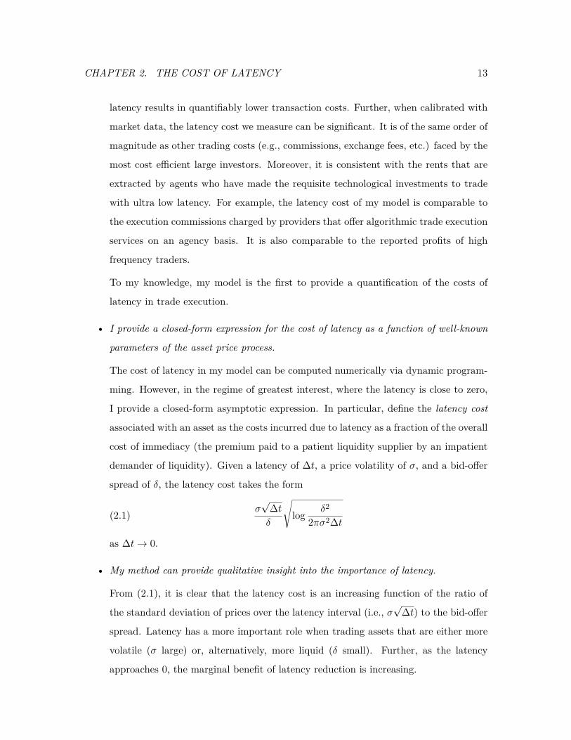
I provide a closed-form asymptotic expression. In particular, define the latency cost
associated with an asset as the costs incurred due to latency as a fraction of the overall
cost of immediacy (the premium paid to a patient liquidity supplier by an impatient
demander of liquidity). Given a latency of ∆t, a price volatility of σ, and a bid-offer
spread of δ, the latency cost takes the form
(2.1) σ√
∆tδ
√log δ2
2πσ2∆t
as ∆t→ 0.
• My method can provide qualitative insight into the importance of latency.
From (2.1), it is clear that the latency cost is an increasing function of the ratio of
the standard deviation of prices over the latency interval (i.e., σ√
∆t) to the bid-offer
spread. Latency has a more important role when trading assets that are either more
volatile (σ large) or, alternatively, more liquid (δ small). Further, as the latency
approaches 0, the marginal benefit of latency reduction is increasing.
CHAPTER 2. THE COST OF LATENCY 14
• This chapter empirically demonstrates that latency cost incurred by trading on a hu-
man time scale has dramatically increased for U.S. equities and the implied latency
of a representative trader in this market decreased by approximately two orders of
magnitude.
I consider the cost due to the latency of trading on the time scale of human interac-
tion.Using the data-set of Aït-Sahalia and Yu [2009], I estimate the latency cost of
NYSE common stocks over the 1995–2005 period. I show that the median latency
cost more than tripled in this time. This coincides with a period of decreasing tick
sizes and increasing algorithmic and high frequency trading activity [Hendershott et
al., 2010].
An alternative perspective is to consider a hypothetical investor who fixes a target level
of cost due to latency, relative to the overall cost-of-immediacy. The representative
trader maintains this target over time through continual technological upgrades to
lower levels of latency. I determine the requisite level of implied latency for such a
trader, over time and across the aggregate market. Using the same data-set, I observe
that the median implied latency decreased by approximately two orders of magnitude
over this time frame.
The rest of this chapter is organized as follows: In Section 4.1.1, I review the related
literature. In Section 2.2, as a starting point, I present a stylized, continuous-time trade
execution problem in the absence of latency. I develop a variation of the model with
latency in Section 4.2. In Section 2.4, I provide a mathematical analysis of the optimal
policy for my problem. By contrasting the results in the presence and absence of latency,
I am able to quantitatively assess the cost of latency. In Section 2.5, I consider some
empirical applications of the model. Finally, in Section 3.6 I conclude and discuss some
future directions.
2.1.1. Related Literature
There has been a significant empirical literature studying, broadly speaking, the effects of
improvements in trading technology. Closest to the aspect I consider is the work of Easley
CHAPTER 2. THE COST OF LATENCY 15
et al. [2008]. They empirically test the hypothesis that latency affects asset prices and
liquidity by examining the time period around an upgrade to the New York Stock Exchange
technological infrastructure that reduced latency. Hendershott et al. [2010] explore the
more general, overall effects of algorithmic and high frequency trading. Hasbrouck and
Saar [2009] provide different evidence of changes in investor trading strategies that may be
a result of improved technology. In subsequent work, they further consider the impact of
measurements of low latency on market quality [Hasbrouck and Saar, 2010]. Hendershott
and Riordan [2009] analyze the impact of algorithmic trading on the price formation process
using a data set from Deutsche Börse and conclude that algorithmic trading assists in the
efficient price discovery without increasing the volatility. Kirilenko et al. [2010] consider the
impact of high frequency trading on the ‘flash crash’ of 2010, while Brogaard [2010] more
broadly examines the impact of high frequency traders on market quality.
On the theoretical front, Cespa and Foucault [2008] consider a rational expectations
equilibrium between investors with different access to past transaction data. Some investors
observe transactions in real-time, while others only observe transactions with a delay. This
model of latency focuses on latency of the price ticker of past transactions, as opposed to
latency in execution, which I consider here. Moreover, the goals of the two models differ
significantly: Cespa and Foucault [2008] seek to build intuition regarding the equilibrium
welfare implications of differential access to information via a structural model. I, on the
other hand, seek a reduced form model that can be used to directly estimate the value of
execution latency in a particular real world instance, given readily available data. Also
related is the work of Ready [1999] and Stoll and Schenzler [2006], who consider the ability
of intermediaries (e.g., specialists or dealers) to delay customer orders for their own benefit,
thus creating a “free option” in the presence of execution latency. Cohen and Szpruch [2011]
show that latency arbitrage exists between two traders with different speeds of trading in
the presence of a limit order book. Finally, Cvitanic and Kirilenko [2010] and Jarrow and
Protter [2011] consider the effect of high frequency traders on asset prices.
The trade execution problem I consider is that of an investor who wishes to sell a
single share of and must decide between market and limit orders. This problem has been
considered by many others [e.g., Angel, 1994; Harris, 1998; Lo et al., 2002]. My formulation

CHAPTER 2. THE COST OF LATENCY 16
is similar to the class of barrier-diffusion models considered by these authors; Hasbrouck
[2007] provides a good account of this line of work. For a broad survey on limit order
markets, see Parlour and Seppi [2008]. In my model, the inability to trade continuously
gives a limit order an option-like quality that relates execution cost, order duration, and
asset volatility. This idea goes as far back as the work of Copeland and Galai [1983].
Closely related is the concept of the cost of immediacy, or, the premium paid by a liquidity
demander via a market order to a liquidity supplier who posts a limit order. Grossman
and Miller [1988] and Chacko et al. [2008] develop theoretical explanations of the cost of
immediacy. For empirical evidence of the demand for immediacy in capital markets, see
Bacidore et al. [2003] and Werner [2003].
Finally, also related is work on the discrete-time hedging of contingent claims with or
without transaction costs [e.g., Boyle and Emanuel, 1980; Leland, 1985; Bertsimas et al.,
2000]. This literature addresses a different problem and draws different conclusions than my
chapter, however both relate to implications of a lack of continuous access to the market.
2.2. A Stylized Execution Model without Latency
My goal is to understand the impact on the trade execution of latency. To this end, I
will first describe a trade execution problem in the absence of latency. In Section 4.2, I
will revisit this model in the presence of latency, so as to understand the resulting trade
friction that is introduced. The spirit of my model it to consider an investor who wants to
trade, but at a price that depends on an informational process that evolves stochastically
and must be monitored continuously. I could directly consider such an abstract model of
investor behavior. Instead, however, I will motivate the informational dependence of the
trader through a specific optimal execution problem.
Consider the following stylized execution problem of an uninformed trader who must
sell exactly one share6 of a stock over a time horizon [0, T ]. At any time t ∈ [0, T ), the
6Note that the trade quantity of a single share is meant to represent an atomic unit of the asset, or
the smallest commonly traded lot size. The underlying assumption is that the desired trade execution will
ultimately be accomplished by a single transaction. In typical U.S. equity markets, for example, this atomic
unit might be a block of 100 shares.

CHAPTER 2. THE COST OF LATENCY 17
trader can take one of two actions:
1. The trader can submit a market order to sell. This order will execute at the best bid
price at time t, denoted by St. I assume that the bid price evolves according to
(2.2) St = S0 + σBt,
where the process (Bt)t∈[0,T ] is a standard Brownian motion and σ > 0 is an (additive)
volatility parameter. Here, the choice of Brownian motion is made for simplicity;
my model can be extended to the more general class of Markovian martingales, as
discussed in Section 2.4.4.
2. The trader can choose to submit a limit order to sell. In this case, the trader must
also decide the limit price associated with the order, which I denoted by Lt.
Once the trader sells one share, he exits the market. If the trader is not able to sell 1 share
before time T , however, I assume that he is forced sell via a market order at time T , and
therefore receives ST . Here, I imagine the time horizon T to be small, on the order of the
typical trade execution time (i.e., seconds).
2.2.1. Limit Order Execution
It remains to describe the execution of limit orders. In my setting, a limit order can execute
in one of the following two ways:
1. I assume that there are impatient buyers who arrive to the market according to a
Poisson process with rate µ. Denote by (Nt)t∈[0,T ) the cumulative arrival process for
impatient buyers. Each impatient buyer seeks to buy a single share. An arriving
impatient buyer arriving at time t has a reservation price St + zt, expressed as a
premium zt ≥ 0 above the bid price St that the buyer is willing to forgo in order
to achieve immediate execution. I assume that the premium zt is independent and
identically distributed with cumulative distribution function F : R+ → [0, 1]. In this
setting, the instantaneous arrival rate of impatient buyers at time t willing to pay a
limit order price of Lt is given by
(2.3) λ(ut) , µ(1− F (ut)),

CHAPTER 2. THE COST OF LATENCY 18
where ut , Lt − St is the instantaneous price premium of the limit order. In what
follows, I will be particularly interested in the special case where
(2.4) λ(ut) ,
µ if ut ≤ δ,
0 otherwise.
Here, I assume that every impatient buyer is willing to pay a price premium of at
most δ > 0. I assume that δ will be specific to the security and fixed for the trading
horizon. I will discuss the extension to the general case (2.3) in Section 2.4.4.
Given (2.4), an impatient buyer is willing to buy 1 share at a fixed premium δ > 0 to
the bid price at the time of their arrival. Hence, if a buyer arrives at time τ ∈ [0, T ),
and the trader has placed a limit order with price Lτ , the limit order will execute if
Lτ ≤ Sτ + δ.
2. Alternatively, a limit order will also execute at time τ if the bid price crosses the limit
order price, i.e., Sτ ≥ Lτ .
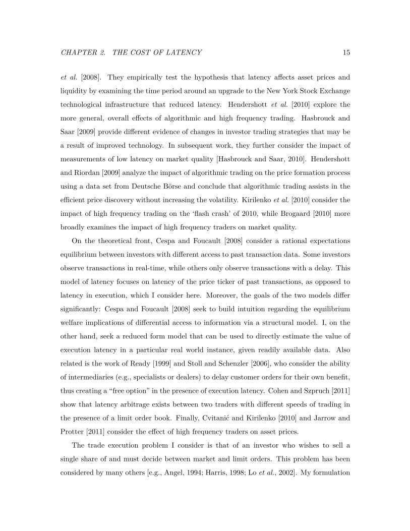
The execution of limit orders in the model is illustrated in Figure 2.1.
The limit order execution dynamics above can also be economically interpreted in the
spirit of the non-informational trade model of Roll [1984]. In particular, imagine that the
asset has a fundamental value Vt at time t, and that Vt evolves exogenously according to
the additive random walk
Vt = V0 + σBt.
If all investors observe this underlying value process and are symmetrically informed, com-
petitive market makers will always be willing to sell shares at a price of δ/2 above the
fundamental value or buy shares at a spread of δ/2 below the fundamental value. Here,
the quantity δ captures the per share operating costs of trade to the market markers. The
liquidating trader can thus sell at the bid price St = Vt − δ/2 at any time t. I assume that
all other traders in the market are impatient, and that these traders arrive according to the
Poisson dynamics described above. An arriving impatient buyer will choose to purchase
from the liquidating trader only at a price lower than that provided by the market makers,
i.e., only below the price of Vt+δ/2 = St+δ. In this way, I can interpret the parameter δ as
CHAPTER 2. THE COST OF LATENCY 19
t0 T
St
Lt
Sτ1 + δ
τ1
Sτ2 + δ
τ2 τ3
market orders arrive
limit order executes
Figure 2.1: An illustration of the limit order execution in the stylized model over the time
horizon [0, T ]. Here, I assume the trader leaves a limit order with the (constant) price Lt and
St is the bid price process. If market orders arrive at times τ1 and τ2, the limit order would
execute at time τ2 but not time τ1, since the limit order price is in excess of δ to the best bid
price. The limit order would also execute at time τ3 in the absence of a market order arrival,
since the bid price crosses the limit order price at this time.
the prevailing bid-offer spread, that is, the bid-offer spread in the absence of the liquidating
trader.
2.2.2. Optimal Solution
Let P denote the random variable associated with the sale price. I assume the trader is
risk-neutral and seeks to maximize the expected sale price. Equivalently, I assume the
trader seeks to solve the optimization problem
(2.5) h0 , maximize E [P ]− S0.
Here, the maximization is over policies of market orders and limit orders which are non-
anticipating, i.e., which are adapted to the filtration generated by (Bt, Nt)t∈[0,T ]. This
objective is equivalent to minimizing implementation shortfall [Perold, 1988].
Note that, while this stylized problem may seem quite simplified, it seeks to answer a
fundamental question: at the level of an atomic unit of stock and over a short time horizon,
how should a risk-neutral investor choose between limit orders and market orders? This
problem is a central ingredient in more sophisticated optimal execution problems involving
CHAPTER 2. THE COST OF LATENCY 20
risk averse investors selling large quantities over longer time horizons.7 This is because, in a
typical algorithmic trading setting, a large “parent” order will be scheduled across time into
many very small “child” orders. Each of these “child” orders need to be executed optimally.
Since each child order is small and since there are many such child orders, it is reasonable
to view the investor as risk-neutral with respect to each child order.
The following lemma characterizes a simple strategy that is optimal for the execution
problem I have described:
Lemma 1. An optimal strategy is to employ only limit orders at times t ∈ [0, T ), with limit
price Lt = St + δ. In other words, the limit order price is “pegged” at a constant premium
δ above the bid price. This pegging strategy achieves the optimal value
(2.6) h0 = δ(1− e−µT
).
Proof. Consider a trader using an arbitrary strategy, and denote by τ ∈ [0, T ] the (random)
time at which the trader sells the share, and by τ1 ∈ [0,∞) the time at which the first
impatient buyer arriving to the market. Let E be the event that the trader sells via a limit
order to an impatient buyer at the price Lτ . Then, under the event Ec, the trader sells at
the bid price Sτ . Then, the sale price P can be written as8
P = Sτ IEc + Lτ IE ≤ Sτ IEc + (Sτ + δ)IE ≤ Sτ + δIτ1<T.(2.7)
Here, for the first inequality, I used the fact that an impatient buyer will only buy at time
τ is Lτ ≤ Sτ + δ, and, for the second inequality, I used the fact that the event E can only
occur if an impatient buyer arrives in the time interval [0, τ). Denote by h0 the value under
an optimal strategy. Using the fact that τ is a bounded stopping time and the fact that Stis a martingale, by the optional sampling theorem,
h0 ≤ E[P ]− S0 ≤ E[Sτ + δIτ1<T]− S0 = δP(τ1 < T ) = δ(1− e−µT
).
On the other hand, the hypothesized strategy results in equality in (2.7). Thus, the result
follows.
7For example, see Bertsimas and Lo [1998] or Almgren and Chriss [2000]. These questions have also
recently been addressed by Back and Baruch [2007] and Pagnotta [2010] in equilibrium settings.8I denote by IE the indicator function of the event E .
CHAPTER 2. THE COST OF LATENCY 21
t0 T
St
Lt
Lt = St + δ
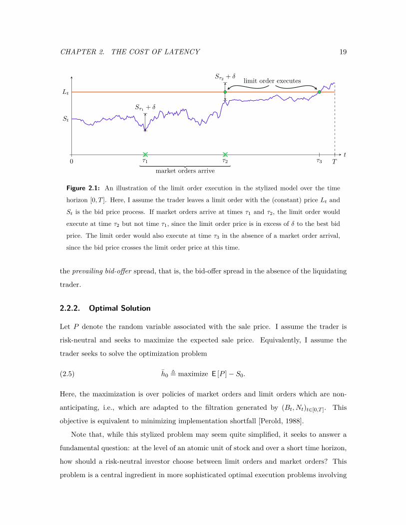
Figure 2.2: An illustration of an optimal strategy with no latency, over the time horizon [0, T ].
The trader uses only limit orders prior to end of the time T . The limit order price Lt is pegged
to the bid price St, with an additional premium corresponding to the bid-offer spread δ.
The optimal pegging strategy suggested by Lemma 1 is illustrated in Figure 2.2. This
policy can be interpreted intuitively as follows: since the trader is risk-neutral and the bid
price process is a martingale, the trader is indifferent between trading at time 0 at the bid
price or trading at any other time at the bid price. Via a limit order, however, the trader
can receive a price which is in excess of the bid price. The excess premium is limited to
δ, since an impatient buyer will not pay more than this. Hence, the trader maintains a
single limit order in the book, and continuously updates the price to track bid price, plus
an additional premium of δ.
Note that my stylized execution model captures only the behavior of a single agent.
My model does not capture the strategic response of other agents, either competing agents
submitting limit orders to sell, or contra-side impatient buyers. Both of these types of agents
might be expected to react to the activity of the limit order trader, and may diminish the
gains of the limit order trader. Separately, my model also exaggerates the gains to be earned
by placing limit orders rather than market orders, due to the fact I do not include adverse
selection costs incurred by limit orders.
However, at a high level, a trader in my model with a mandate to trade over a fixed time
horizon but with no private information as to the asset value prefers limit orders to market
orders. I believe this is representative of the situation of algorithmic traders executing large
“parent” orders in practice. When executing a “child” order over a short time horizon,

CHAPTER 2. THE COST OF LATENCY 22
such traders typically first submit limit orders, and then “clean up” with market orders as
time runs short. Hence, despite omissions of strategic considerations and other significant
simplifications, the resulting policies do capture representative features of real world trading,
if only at a stylized level. Moreover, my simplified single-agent mode enables us to address
the dynamic nature of trade execution and obtain a closed-form expression highlighting the
exact drivers of the latency cost.
2.3. A Model for Latency
The optimal policy for the stylized execution problem of Section 2.2 relied on the ability
of a trader to continuously track an informational process, namely, the bid price in the
market, and to update his order as the process evolves. Here, I will consider a variation
of that problem where the trader is unable to continuously participate in the market, but
faces a fixed latency ∆t > 0. 9 I am interested in quantifying the cost of this latency by
comparing the expected payoff in this model to that in the stylized model without latency.
Note that the model at hand is quite basic with regards to some of primitives (e.g., the
stochastic process describing the evolution of bid prices), I will discuss a number of tractable
extensions in Section 2.4.4, including more complicated models of the bid price process and
of limit order execution.
In general, latency that a trader experiences can take many forms. Minimally, for
example, there is the delay of the data feeds that deliver market price information to the
trader. There is the delay of the trader’s own decision making. Finally, there is the delay
of the trader’s resulting order reaching the marketplace. I assume that the trader makes
decisions instantaneously — we will see that this is reasonable since the optimal decision
rule for the trader will take a very simple form. Further, from the trader’s perspective, the
roundtrip delay (the total delay for an order to be processed by an exchange and reflected in
9Note that many modern exchanges explicitly allow for pegged orders; these orders obviate the need
for the trader to continually track the bid price in the manner I describe. However, more generally, when
tracking an alternative informational process such as the price on a different exchange, the fundamental
value (see Section 2.2), etc., a trader would still need to continuously monitor the market relative to the
informational process, and latency would be important.
CHAPTER 2. THE COST OF LATENCY 23
T0 = 0 Ti = i∆t Ti+1 Ti+2 T = n∆t· · · · · ·
`i−1`i
`i+1
`0 `i `i+1 `i+2
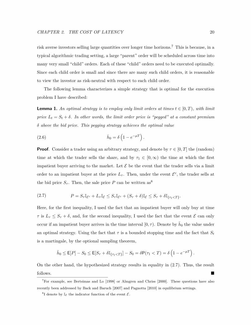
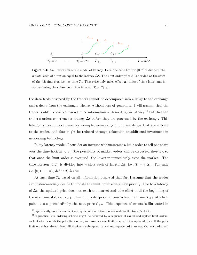
Figure 2.3: An illustration of the model of latency. Here, the time horizon [0, T ] is divided into
n slots, each of duration equal to the latency ∆t. The limit order price `i is decided at the start
of the ith time slot, i.e., at time Ti. This price only takes effect ∆t units of time later, and is
active during the subsequent time interval [Ti+1, Ti+2).
the data feeds observed by the trader) cannot be decomposed into a delay to the exchange
and a delay from the exchange. Hence, without loss of generality, I will assume that the
trader is able to observe market price information with no delay or latency,10 but that the
trader’s orders experience a latency ∆t before they are processed by the exchange. This
latency is meant to capture, for example, networking or routing delays that are specific
to the trader, and that might be reduced through colocation or additional investment in
networking technology.
In my latency model, I consider an investor who maintains a limit order to sell one share
over the time horizon [0, T ] (the possibility of market orders will be discussed shortly), so
that once the limit order is executed, the investor immediately exits the market. The
time horizon [0, T ] is divided into n slots each of length ∆t, i.e., T = n∆t. For each
i ∈ 0, 1, . . . , n, define Ti , i∆t.
At each time Ti, based on all information observed thus far, I assume that the trader
can instantaneously decide to update the limit order with a new price `i. Due to a latency
of ∆t, the updated price does not reach the market and take effect until the beginning of
the next time slot, i.e., Ti+1. This limit order price remains active until time Ti+2, at which
point it is superseded11 by the next price `i+1. This sequence of events is illustrated in10Equivalently, we can assume that my definition of time corresponds to the trader’s clock.11In practice, this ordering scheme might be achieved by a sequence of cancel-and-replace limit orders,
each of which cancels the prior limit order, and inserts a new limit order with the updated price. If the prior
limit order has already been filled when a subsequent cancel-and-replace order arrives, the new order will
CHAPTER 2. THE COST OF LATENCY 24
Figure 2.3. Between the time Ti, when the price `i is decided, and the time Ti+1, when the
updated order reaches the market, the following events can occur:
• E(1)i : An impatient buyer arrives in the time interval (Ti, Ti+1) and `i−1 ≤ STi + δ,
i.e., the prior limit price `i−1, which is active at that time, is within a margin δ of
the bid price at the start of the interval. In this case, the limit order executes at the
price `i−1, and the investor leaves the market. Note that the updated limit price `inever takes effect.
I assume that the probability that an impatient buyer arrives in any given time slot
is µ∆t, and that these arrivals occur independently of everything else.12 I assume
that ∆t < 1/µ so that this probability is well-defined. The bid price process evolves
according to the random walk (2.2).
• E(2)i : Otherwise, if STi+1 ≥ `i, i.e., the bid price has crossed the order price `i at the
instant the order reaches the market, then the order immediately executes at price
STi+1 .
• E(3)i : Otherwise, the limit order price `i is active over the time interval [Ti+1, Ti+2).
In order to consider the possibility of market orders, I allow the limit price `i = −∞.
By picking this price, the trader can guarantee that the bid price at time Ti+1 will cross the
order price, i.e., STi+1 ≥ `i with probability 1. Thus, the choice of `i = −∞ corresponds to a
certain execution at the bid price STi+1 , i.e., a market order. Similarly, the trader can make
the decision at time Ti not to trade by setting `i =∞. As in the model of Section 2.2, if the
investor has been unable to sell the share by the end of the time horizon T , the investor is
forced to sell via a ‘clean-up’ trade, i.e., a market order at time T . This is accomplished by
enforcing the constraint that `n−1 = −∞, which I will assume implicitly in what follows.
As before, if P is the random variable associated with the sale price, the trader is
risk-neutral and seeks to solve the optimization problem
(2.8) h0(∆t) , maximize`0,...,`n−1
E [P ]− S0.
fail. Hence, the investor is guaranteed to sell at most one share.12Note that this is simply a discrete-time Bernoulli arrival process that is analogous to the the Poisson
arrival process of Section 2.2.
CHAPTER 2. THE COST OF LATENCY 25
Here, the maximization is over the choice of limit order prices (`0, `1, . . . , `n−1). I assume
that the price decisions are non-anticipating, i.e., each `i is adapted to the filtration gener-
ated by the bid price process and the arrival of impatient buyers up to and including time
Ti. My goal is to analyze h0(∆t), which is the value under an optimal trading strategy
when the latency is ∆t.
Note that, as compared to the model of Section 2.2, my present model with latency differs
in two ways: First, the trader makes decisions at the beginning of discrete-time intervals of
length ∆t, as opposed to continuously. Second, the orders of the trader incur a latency or
delay of length ∆t before they reach the marketplace. I am interested in studying the impact
of the latter feature, latency, and I adopt the former feature, discrete-time decision making,
so as to admit a tractable dynamic programming analysis. In Section 2.4.3, however, we
will see that in the low latency regime in which we are most interested, the discrete-time
nature of my model has a negligible impact.
2.4. Analysis
In this section, I solve for the optimal policy for the trader in the latency model of Sec-
tion 4.2. This problem can be solved via a dynamic programming decomposition that is
presented in Section 2.4.1. While the exact dynamic programming solution can be com-
puted numerically, in Section 2.4.2 I will present an asymptotic analysis that provides a
closed-form analytic expression for the cost of latency in the low latency regime, where
∆t→ 0. In Section 2.4.3, I will consider the implications of the discrete-time nature of my
latency model. Finally, in Section 2.4.4, I will discuss a number of extensions of my latency
model.
2.4.1. Dynamic Programming Decomposition
The standard approach to solving the optimal control problem (2.8) is to employ dynamic
programming arguments. In Appendix A.1, I formally derive the optimal control policy
using these methods. In order to focus on the high level picture, however, for the moment
I will be content with summarizing those results.
CHAPTER 2. THE COST OF LATENCY 26
In particular, assume a fixed latency of ∆t. For each decision time Ti with 0 ≤ i < n,
define Ui to be the event that the trader’s limit order remains unfulfilled prior to time Ti+1,
i.e., none of the orders submitted at prices `0, . . . , `i−1 are executed. Note that if the event
Ui does not hold, then the limit order price `i to be decided at time Ti is irrelevant. This is
because, by the time that order arrives to the market, the trader would have already sold
a share. Define the quantity
(2.9) hi , maximize`i,...,`n−1
E [P | STi , Ui]− STi .
Note that h0 = h0(∆t), where h0(∆t) is defined in (2.8), and thus my notation is consistent.
More generally, for i > 0, I can interpret hi to be the trader’s expected payoff at time Tirelative to the current bid price STi under the optimal policy, the order does not get filled
prior to time Ti+1. Thus, hi can be interpreted as a continuation value in the dynamic
programming context.
The continuation values hi quantify the remaining value for a trader at each time
period if his order remains unfulfilled. Given the continuation values, at each time Ti,
the investor can make an optimal decision as to the limit order price `i by balancing the
benefits of execution in the time slot [Tt+1, Ti+2) with the value hi+1 that will be obtained
if the order is not executed. Moreover, the optimal decisions and continuation values can be
jointly computed via backward induction of a Bellman equation. This result is captured in
the following theorem. The proof, which is provided in Appendix A.1, follows from formal
dynamic programming arguments.
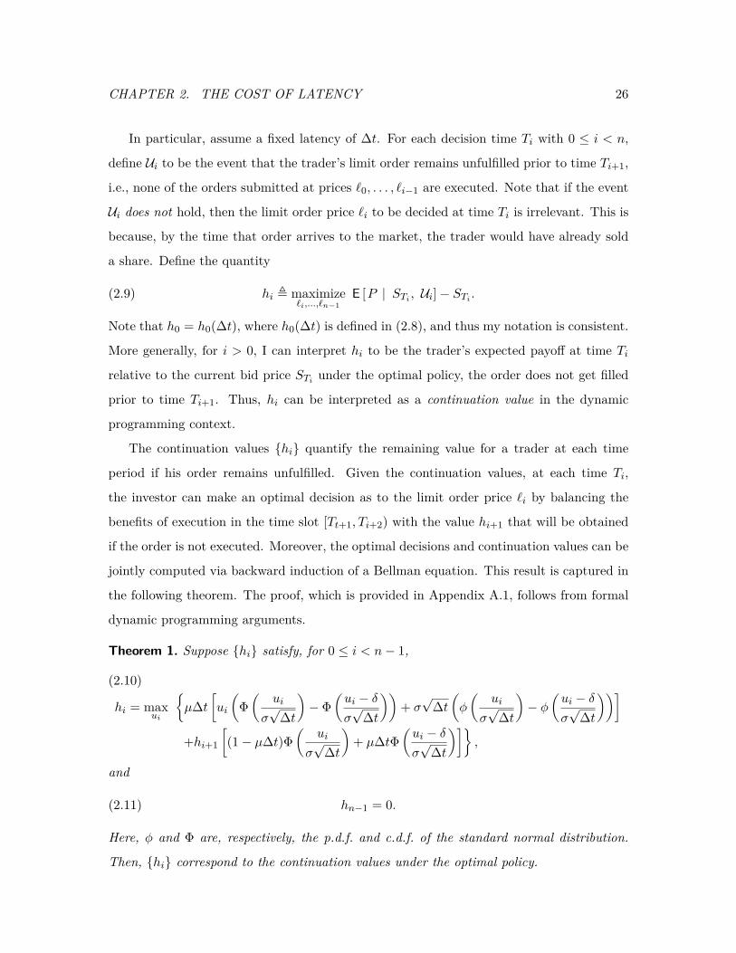
Theorem 1. Suppose hi satisfy, for 0 ≤ i < n− 1,
hi = maxui
µ∆t
[ui
(Φ(
ui
σ√
∆t
)− Φ
(ui − δσ√
∆t
))+ σ√
∆t(φ
(ui
σ√
∆t
)− φ
(ui − δσ√
∆t
))]+hi+1
[(1− µ∆t)Φ
(ui
σ√
∆t
)+ µ∆tΦ
(ui − δσ√
∆t
)],
(2.10)
and
(2.11) hn−1 = 0.
Here, φ and Φ are, respectively, the p.d.f. and c.d.f. of the standard normal distribution.
Then, hi correspond to the continuation values under the optimal policy.
CHAPTER 2. THE COST OF LATENCY 27
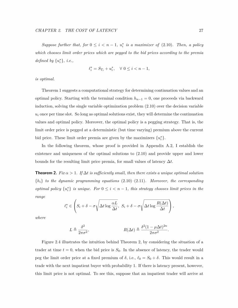
Suppose further that, for 0 ≤ i < n − 1, u∗i is a maximizer of (2.10). Then, a policy
which chooses limit order prices which are pegged to the bid prices according to the premia
defined by u∗i , i.e.,
`∗i = STi + u∗i , ∀ 0 ≤ i < n− 1,
is optimal.
Theorem 1 suggests a computational strategy for determining continuation values and an
optimal policy. Starting with the terminal condition hn−1 = 0, one proceeds via backward
induction, solving the single variable optimization problem (2.10) over the decision variable
ui once per time slot. So long as optimal solutions exist, they will determine the continuation
values and optimal policy. Moreover, the optimal policy is a pegging strategy. That is, the
limit order price is pegged at a deterministic (but time varying) premium above the current
bid price. These limit order premia are given by the maximizers u∗i .
In the following theorem, whose proof is provided in Appendix A.2, I establish the
existence and uniqueness of the optimal solutions to (2.10) and provide upper and lower
bounds for the resulting limit price premia, for small values of latency ∆t.
Theorem 2. Fix α > 1. If ∆t is sufficiently small, then there exists a unique optimal solution
hi to the dynamic programming equations (2.10)–(2.11). Moreover, the corresponding
optimal policy u∗i is unique. For 0 ≤ i < n − 1, this strategy chooses limit prices in the
range
`∗i ∈
Si + δ − σ
√∆t log αL∆t , Si + δ − σ
√∆t log R(∆t)
∆t
,where
L ,δ2
2πσ2 , R(∆t) , δ2(1− µ∆t)2n
2πσ2 .
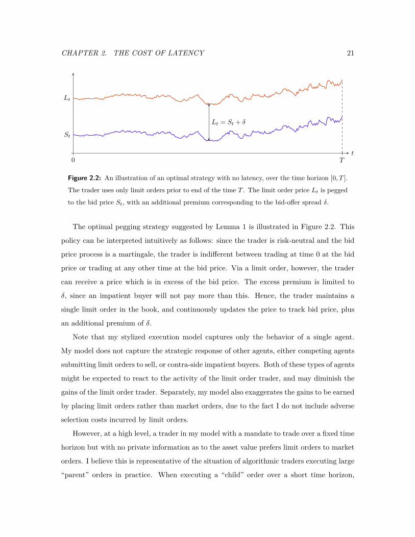
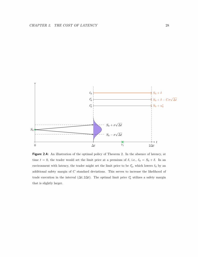
Figure 2.4 illustrates the intuition behind Theorem 2, by considering the situation of a
trader at time t = 0, when the bid price is S0. In the absence of latency, the trader would
peg the limit order price at a fixed premium of δ, i.e., `0 = S0 + δ. This would result in a
trade with the next impatient buyer with probability 1. If there is latency present, however,
this limit price is not optimal. To see this, suppose that an impatient trader will arrive at
CHAPTER 2. THE COST OF LATENCY 28
t0 ∆t 2∆tτ1
S0
S0 + σ√
∆t
S0 − σ√
∆t
`0 S0 + δ
`′0 S0 + δ − Cσ√
∆t
`∗0 S0 + u∗0
Figure 2.4: An illustration of the optimal policy of Theorem 2. In the absence of latency, at
time t = 0, the trader would set the limit price at a premium of δ, i.e., `0 = S0 + δ. In an
environment with latency, the trader might set the limit price to be `′0, which lowers `0 by an
additional safety margin of C standard deviations. This serves to increase the likelihood of
trade execution in the interval (∆t, 2∆t). The optimal limit price `∗0 utilizes a safety margin
that is slightly larger.
CHAPTER 2. THE COST OF LATENCY 29
time τ1 ∈ (∆t, 2∆t). If the limit order price is set at `0, the probability that the trade does
not get executed is
P (`0 ≥ S∆t + δ) = P (S0 ≥ S∆t) = 1/2.
When ∆t is small, the probability of missing an execution can be significantly lowered at a
small cost by lowering `0 by an additional safety margin. If we set this safety margin to be
C standard deviations of the one-period price change, i.e., `′0 = S0 + δ − Cσ√
∆t, then the
probability of missing execution becomes
P(`′0 ≥ S∆t + δ
)= P
(S0 − Cσ
√∆t ≥ S∆t
)= Φ(−C).
This probability can be made close to 0 by the choice of C. However, given a fixed choice
of C independent of ∆t, the probability remains constant (i.e., independent of ∆t) and
non-zero. The additional safety margin corresponding to the log term in Theorem 2 is a
second order adjustment. This is introduced so that, given the optimal limit price `∗0, the
probability of execution tends to 1 as ∆t→ 0.
2.4.2. Asymptotic Analysis
The dynamic programming decomposition developed in Section 2.4.1 allows the exact nu-
merical computation of the value h0(∆t), the value under an optimal policy of the latency
model introduced in Section 4.2, when the latency is ∆t. As discussed earlier, the latency
observed in modern electronic markets is extremely small, often on the time scale of millisec-
onds. Thus, we are most interested in the qualitative behavior of h0(∆t) in the asymptotic
regime where ∆t→ 0. The main result of this section is the following theorem, whose proof
is provided in Appendix A.3. It provides a closed-form expression for h0(∆t), which holds
asymptotically13 as ∆t→ 0.13In what follows, given arbitrary functions f and g, and a positive function q, I will say that f(∆t) =
g(∆t) + O(q(∆t)) if lim sup∆t→0 |f(∆t) − g(∆t)|/q(∆t) < ∞, i.e., if the difference between f and g, as
∆t→ 0, is asymptotically bounded above by some positive multiple of q. Similarly, I will say that f(∆t) =
g(∆t) + o(q(∆t)) if lim∆t→0 |f(∆t)− g(∆t)|/q(∆t) = 0, i.e., if the difference between f and g, as ∆t→ 0, is
asymptotically dominated by every positive multiple of q. Finally, I will say that f(∆t) = g(∆t) + Θ(q(∆t))
if 0 < lim inf∆t→0 |f(∆t) − g(∆t)|/q(∆t) ≤ lim sup∆t→0 |f(∆t) − g(∆t)|/q(∆t) < ∞, i.e., if the difference
between f and g is asymptotically bounded above and below by positive multiples of q.
CHAPTER 2. THE COST OF LATENCY 30
Theorem 3. As ∆t→ 0,
h0(∆t) = h0
1− σ
δ
√∆t log δ2
2πσ2∆t
+ o(√
∆t),
where
h0 = δ(1− e−µT
)is the optimal value for the stylized model without latency, i.e., the value defined by (2.5).
Theorem 3 is not surprising when considered in the context of Theorem 2. In the stylized
model without latency, the optimal strategy is to peg the limit order price at a premium
of δ, and this yields a value of h0. On the other hand, Theorem 2 suggests a trader facing
latency ∆t will lower this limit price premium by a factor of, approximately,
σ
δ
√∆t log δ2
2πσ2∆t + o(√
∆t).
If this lowers the ultimate value proportionally, then the value of the optimal policy in the
presence of latency ∆t should approximately be
h0
1− σ
δ
√∆t log δ2
2πσ2∆t
+ o(√
∆t).
The proof of Theorem 3, provided in Appendix A.3, makes this intuition precise.
One implication of Theorem 3 is that h0(∆t) → h0 as ∆t → 0, i.e., the value of the
latency model converges to that of the stylized model without latency of Section 2.2. This
suggests the following definition:
Definition 1. Define the latency cost associated with latency ∆t by
(2.12) LC(∆t) , h0 − h∗0(∆t)h0
.
Latency cost has an easy interpretation. Using h0, the value obtained in the stylized
model without latency as a benchmark, the numerator of (2.12) is the lost revenue incurred
due the the presence of latency. On the other hand, we can regard the denominator as
the cost of immediacy for an impatient investor in a time horizon of length T . This is
because, in the stylized model without latency, it is the difference in revenue obtained by
CHAPTER 2. THE COST OF LATENCY 31
a risk-neutral investor willing to patiently provide liquidity by employing limit orders over
the length of the time horizon, and an impatient investor who demands immediate liquidity
and sells at the bid price at time t = 0, cf. (2.5). Therefore, we can describe the latency cost
as the amount a trader forgoes due to latency, as a percentage of the cost of immediacy.
The following corollary restates the asymptotic approximation of Theorem 3 in terms
of latency cost.
Corollary 1. As ∆t→ 0,
LC(∆t) = σ√
∆tδ
√log δ2
2πσ2∆t + o(√
∆t).
There are a number of interesting observations that can be made regarding the asymp-
totic approximation of Corollary 1. First of all, asymptotically, latency cost does not depend
on the length of the time horizon T or the arrival rate of impatient traders µ. As a function
of the remaining parameters, the asymptotic latency cost depends only on a composite pa-
rameter that is the ratio the one-period standard deviation of price changes σ√
∆t to the
bid-offer spread δ. Both of these quantities are readily measurable empirically. Corollary 1
suggests that the latency cost increasing in this ratio. Thus, at the same level of latency,
the latency cost is most significant for assets which are very volatile or very liquid. Further,
Corollary 1 suggests that, when latency is low, there are increasing marginal benefits to
further reductions in latency, i.e., LC′′(∆t) < 0. In Section 2.5.1, I illustrate some of facts
numerically, as well as considering the accuracy of my approximation, as compared to the
exact latency cost.
2.4.3. Discreteness of Time vs. Latency
The latency model introduced in Section 4.2 differs from the the stylized model without
latency of Section 2.2 in two principal ways: (i) the trader faces a delay or latency between
the time that trading decisions are made and when they reach the marketplace, and (ii)
the latency model is formulated in discrete-time rather than continuous time. The latter
point refers to the facts that, in the model with latency, a trader is only able to update his
limit order at discrete intervals of time rather than continuously, impatient buyers arrive
according to a Bernoulli process rather than a Poisson process, etc. In order to disentangle

CHAPTER 2. THE COST OF LATENCY 32
these two effects, in this section I will briefly describe a trading model that is formulated in
discrete time but without latency. By considering this model, I will demonstrate that the
asymptotic latency cost derived in Section 2.4.2 is indeed due to latency effects and not due
to the discreteness of time.
To this end, consider a model in the discrete-time setting of Section 4.2 but with no
latency. Here, at each time Ti , i∆t, for i = 0, 1, . . . , n, the investor sets a limit order
price `i. This limit order price takes effect immediately. Between time Ti and time Ti+1 the
following events can occur:
• If STi ≤ `i, i.e., the bid price is less than the limit order price, the limit order imme-
diately executes at the price STi .
• Otherwise, suppose that an impatient buyer arrives in the time interval (Ti, Ti+1) and
`i ≤ STi + δ, i.e., the limit price `i is within a margin δ of the bid price at the start
of the interval. In this case, the limit order executes at the price `i. I assume that an
impatient buyer arrives with probability µ∆t, independent of everything else.
As before, if the investor is unable to sell the share by the end of the time interval, he is
forced to sell via a market order, i.e., `n = −∞. If P is the sale price, the optimal value for
the trader in this discrete model is given by
hD0 (∆t) , maximize
`0,...,`nE [P ]− S0.
I have the following result, whose proof is identical to the martingale argument used to
establish Lemma 1.
Lemma 2. An optimal strategy for the discrete model is to place limit orders at the price
`i = STi + δ, for i = 0, 1, . . . , n− 1. This strategy achieves the value
hD0 (∆t) , δ (1− (1− µ∆t)n ).
Now, note that, for all 0 < ∆t < 1/µ,
e−µT−12µ
2T∆t ≤ (1− µ∆t)T/∆t ≤ e−µT .
CHAPTER 2. THE COST OF LATENCY 33
Therefore, the difference in value between the continuous model of Section 2.2 and the
discrete model considered here is at most
|hD0 (∆t)− h0 | ≤ δe−µT
(1− e−
12µ
2T∆t)≤ 1
2δµ2Te−µT∆t.
In other words, this difference is asymptotically O(∆t). By Theorem 3, however, the dif-
ference between the continuous model and the latency model is asymptotically
Θ(√
∆t log(1/∆t)).
Hence, the asymptotic effect of latency dominates the asymptotic effect of the discreteness
of time.
2.4.4. Extensions
The analysis of the latency model that I have presented proceeded according to two high
level steps:
(i) First, in Section 2.4.1, a simplified dynamic programming decomposition was devel-
oped. In this decomposition, at each time, the trader’s value function is parameterized
by a single scalar, rather than being an arbitrary function of state. This allows the
Bellman equation to be solved through a system of n equations in n unknowns, given
by (2.10)–(2.11).
(ii) Second, in Section 2.4.2, an asymptotic analysis of the simplified dynamic program-
ming equations (2.10)–(2.11) was performed. This gave rise to the asymptotic latency
cost expression of Corollary 1.
The dynamic programming decomposition step (i) that is at the heart of my analysis can
be extended to a much broader set of stochastic primitives than the present setting. In each
of these cases, a different set of simplified dynamic programming equations, analogous to
(2.10)–(2.11) would arise, and would require a customized variation of asymptotic analysis
step (ii). In particular, consider the following tractable generalizations:
• Price process. In my model, the price process St is a Brownian motion. My dynamic
programming decomposition only requires that the St be a Markov process and a
CHAPTER 2. THE COST OF LATENCY 34
martingale. It would be straightforward to extend the dynamic programming step (i)
and consider other Markovian martingales, for example, allowing for non-Gaussian
processes, time-inhomogeneous volatility, or for jump processes.
On the other hand, the asymptotic analysis step (ii) I have presented is quite sensi-
tive to distributional assumptions of the price process, and would require specialized
analysis for any such generalization. In Appendix A.4, I consider one generalization
of particular interest, where the price dynamics also contain a jump component.
• Limit order execution. In my model, the execution of a limit order in the time slot
(Ti, Ti+1) required that the limit order price `i−1 be within a spread δ of the bid price
STi , and that an impatient trader arrive. More generally, my dynamic programming
decomposition only requires that the execution of this limit order, conditional on the
price difference `i−1− STi , be independent of everything else. This can accommodate
a number of generalizations, for example, the arrival rate of impatient buyers can
be time-varying. Further, the maximum premium above the bid price St that an
impatient buyer is willing to pay can be randomly distributed, as in (2.3). This would
allow models where a limit order that is priced aggressively low has a much higher
probability of execution. Such models could alternatively be interpreted, as discussed
in Section 2.2, as cases where the prevailing bid-offer spread is not constant, but is
independent and identically distributed, varying from period to period.
2.5. Empirical Estimation of Latency Cost
In this section, I will consider empirical applications of my model. First, I will illustrate the
optimal trading policy and the corresponding value function when the model parameters
are estimated from high frequency market data for a single stock. I will also compare the
exact latency cost (numerically computed via dynamic programming) to the approximation
provided by Corollary 1 in order to access the quality of my approximation. Subsequently,
I show the historical evolution of latency cost and implied latency across a range of U.S.
equities using cross-sectional data on volatilities and bid-offer spreads during the 1995–2005
period.

CHAPTER 2. THE COST OF LATENCY 35
My empirical analysis should be regarded as a first-order study to obtain a rough cali-
bration of my model. It will allow us to analyze the model in relevant parameter regimes,
as well as gaining a broad understanding the implications of my model for the trading of
U.S. equities. My empirical measurement of latency cost requires estimates of, in particular,
the high frequency price volatility σ and the prevailing bid-offer spread δ. Here, I make
a number of simplifications and rely on the recent empirical work of Aït-Sahalia and Yu
[2009] to obtain these quantities:
• I estimate price volatility σ using the maximum likelihood estimates of the volatility
of returns provided by Aït-Sahalia and Yu [2009]. Note that this estimation of high
frequency volatility aims to filter out the impact of microstructure noise and obtain an
unbiased estimate of daily volatility. However, for an investor with a trading horizon
of 1 second, microstructure noise needs to be incorporated as well. Therefore, the high
frequency volatility estimate that is used in my empirical analysis underestimates the
actual volatility faced by a high frequency trader with a very short trading horizon.
• Recall that the prevailing bid-offer spread, δ, equals the bid-offer spread in the absence
of the liquidating trader. In the empirical data, it is impossible to disentangle the
presence of liquidating traders. Moreover, the bid-offer spread will not be constant,
but will vary over the course of the trading day. As a proxy for δ, I use the average
bid-offer spread over the trading day.
Despite these shortcomings, I believe that my empirical analysis can shed light on the
importance of latency in the trading of U.S. equities.
2.5.1. The Optimal Policy and the Approximation Quality
In what follows, I will numerically evaluate the optimal policy in my model, the correspond-
ing value function, and the latency cost approximation. These numerical experiments are
meant to be illustrative of my model. I will use realistic model parameters estimated from
recent market data for a single stock. My methodology here is not meant to be authoritative
— there are many subtleties in the analysis of high frequency data; these are beyond the
scope of the work at hand. However, I do seek to demonstrate that my model parameters
CHAPTER 2. THE COST OF LATENCY 36
can be readily derived from commonly available data.
Specifically, the model parameters herein are estimated from trade-and-quote (TAQ)
data for a stock that is a representative example of a liquid name, Goldman Sachs Group,
Inc. (NYSE: GS), on the trading day of January 4, 2010. This data was obtained from the
Wharton Research and Data Services (WRDS) consolidated TAQ database. Only trades
and quotes originating from the primary exchange (NYSE) during regular trading hours
were considered. The model parameters were estimated as follows:
• Initial bid price: SGS0 = $170.00. This was chosen to be the first transaction price on
the trading day.
• Bid-offer spread: δGS = $0.058, i.e., equivalently, 3.4 basis points relative to the initial
price SGS0 . This was estimated by computing the average spread between bid and offer
quotes over the course of the trading day and rounding to the nearest cent.
• Arrival rate of market orders: µGS = 12.03 (per minute). This was estimated by
dividing the total number of NYSE trades by the length of the trading day.
• Price volatility: σGS = $1.92 (daily), i.e., approximately equivalent to an annualized
volatility of returns of 17.9%. These were estimated from the time series of transaction
prices over the course of the trading day, using maximum likelihood estimation as
described inAït-Sahalia and Yu [2009].
• Trading horizon: T = 10 (seconds).
Figure 2.5 illustrates the optimal limit order policy for GS under different values of
latency. If there is no latency, the limit orders are submitted at a constant premium of
δ. When there is latency, the optimal order policy is obtained using the exact dynamic
programming solution of (2.10)–(2.11). As the latency increases, the limit order premium
is reduced below δ so as to account for the increasing uncertainty of price movements over
the latency interval. Theorem 2 suggests that this reduction is approximately equal to
(2.13) σ
√∆t log δ2
2πσ2∆t .
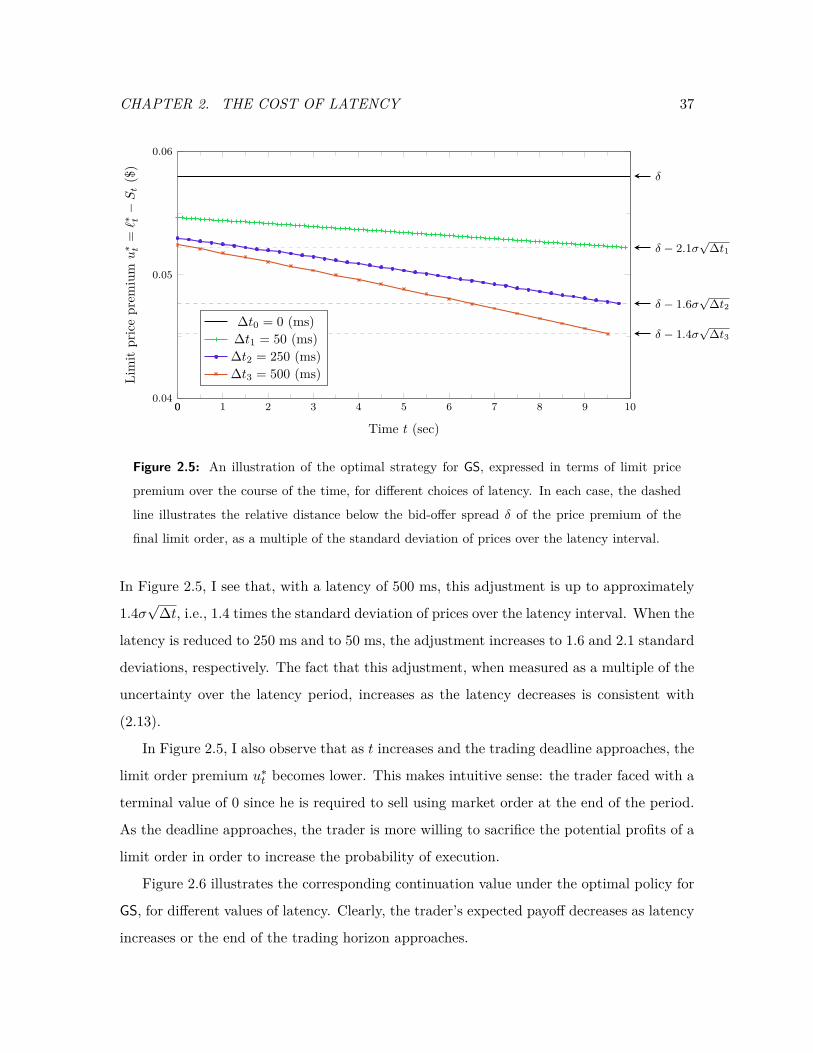
CHAPTER 2. THE COST OF LATENCY 37
0 1 2 3 4 5 6 7 8 9 100.04
0.05
0.06
0
δ
δ − 2.1σ√
∆t1
δ − 1.6σ√
∆t2
δ − 1.4σ√
∆t3
Time t (sec)
Lim
itpr
ice
prem
iumu∗ t
=`∗ t−St
($)
∆t0 = 0 (ms)∆t1 = 50 (ms)∆t2 = 250 (ms)∆t3 = 500 (ms)
Figure 2.5: An illustration of the optimal strategy for GS, expressed in terms of limit price
premium over the course of the time, for different choices of latency. In each case, the dashed
line illustrates the relative distance below the bid-offer spread δ of the price premium of the
final limit order, as a multiple of the standard deviation of prices over the latency interval.
In Figure 2.5, I see that, with a latency of 500 ms, this adjustment is up to approximately
1.4σ√
∆t, i.e., 1.4 times the standard deviation of prices over the latency interval. When the
latency is reduced to 250 ms and to 50 ms, the adjustment increases to 1.6 and 2.1 standard
deviations, respectively. The fact that this adjustment, when measured as a multiple of the
uncertainty over the latency period, increases as the latency decreases is consistent with
(2.13).
In Figure 2.5, I also observe that as t increases and the trading deadline approaches, the
limit order premium u∗t becomes lower. This makes intuitive sense: the trader faced with a
terminal value of 0 since he is required to sell using market order at the end of the period.
As the deadline approaches, the trader is more willing to sacrifice the potential profits of a
limit order in order to increase the probability of execution.
Figure 2.6 illustrates the corresponding continuation value under the optimal policy for
GS, for different values of latency. Clearly, the trader’s expected payoff decreases as latency
increases or the end of the trading horizon approaches.
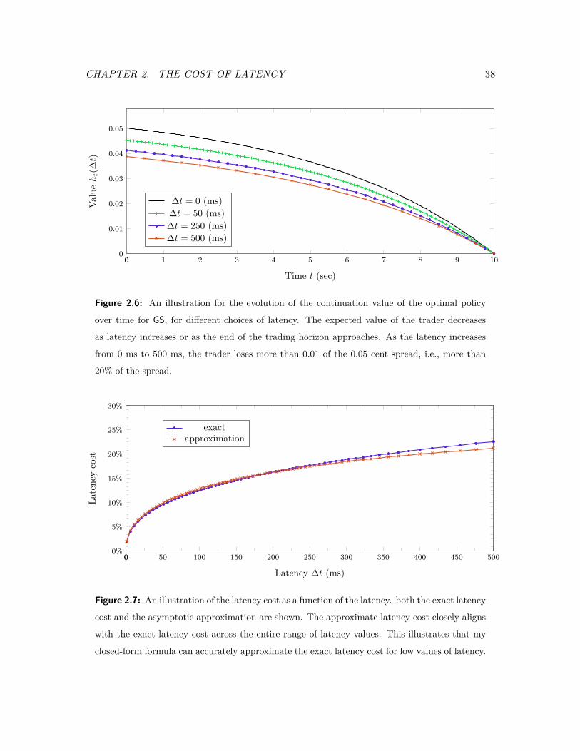
CHAPTER 2. THE COST OF LATENCY 38
0 1 2 3 4 5 6 7 8 9 100
0.01
0.02
0.03
0.04
0.05
0
Time t (sec)
Valu
eht(∆t)
∆t = 0 (ms)∆t = 50 (ms)∆t = 250 (ms)∆t = 500 (ms)
Figure 2.6: An illustration for the evolution of the continuation value of the optimal policy
over time for GS, for different choices of latency. The expected value of the trader decreases
as latency increases or as the end of the trading horizon approaches. As the latency increases
from 0 ms to 500 ms, the trader loses more than 0.01 of the 0.05 cent spread, i.e., more than
20% of the spread.
0 50 100 150 200 250 300 350 400 450 5000%
5%
10%
15%
20%
25%
30%
0
Latency ∆t (ms)
Late
ncy
cost
exactapproximation
Figure 2.7: An illustration of the latency cost as a function of the latency. both the exact latency
cost and the asymptotic approximation are shown. The approximate latency cost closely aligns
with the exact latency cost across the entire range of latency values. This illustrates that my
closed-form formula can accurately approximate the exact latency cost for low values of latency.
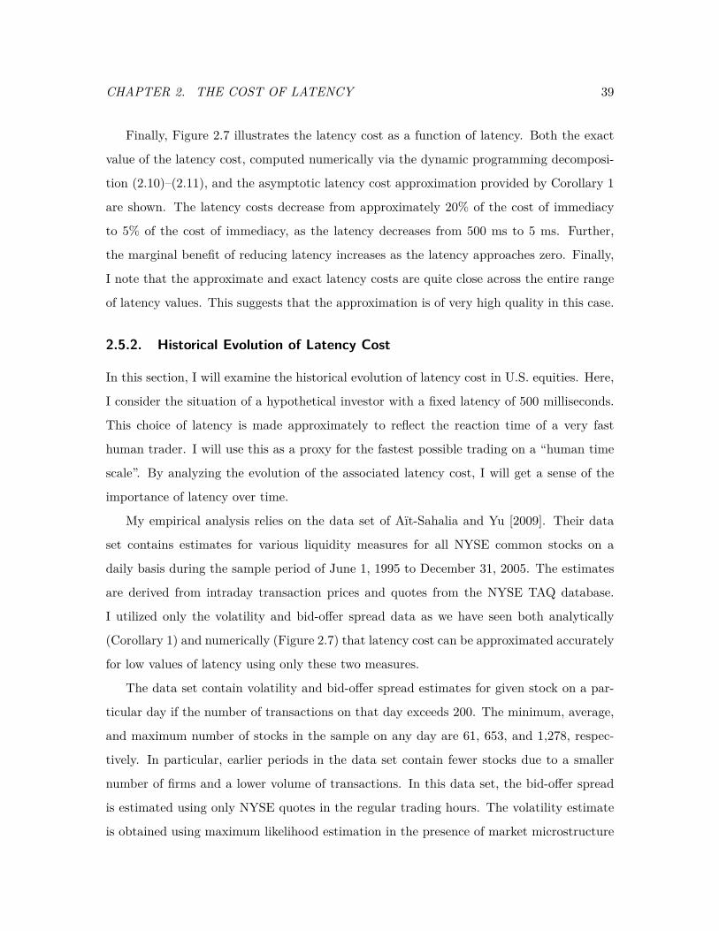
CHAPTER 2. THE COST OF LATENCY 39
Finally, Figure 2.7 illustrates the latency cost as a function of latency. Both the exact
value of the latency cost, computed numerically via the dynamic programming decomposi-
tion (2.10)–(2.11), and the asymptotic latency cost approximation provided by Corollary 1
are shown. The latency costs decrease from approximately 20% of the cost of immediacy
to 5% of the cost of immediacy, as the latency decreases from 500 ms to 5 ms. Further,
the marginal benefit of reducing latency increases as the latency approaches zero. Finally,
I note that the approximate and exact latency costs are quite close across the entire range
of latency values. This suggests that the approximation is of very high quality in this case.
2.5.2. Historical Evolution of Latency Cost
In this section, I will examine the historical evolution of latency cost in U.S. equities. Here,
I consider the situation of a hypothetical investor with a fixed latency of 500 milliseconds.
This choice of latency is made approximately to reflect the reaction time of a very fast
human trader. I will use this as a proxy for the fastest possible trading on a “human time
scale”. By analyzing the evolution of the associated latency cost, I will get a sense of the
importance of latency over time.
My empirical analysis relies on the data set of Aït-Sahalia and Yu [2009]. Their data
set contains estimates for various liquidity measures for all NYSE common stocks on a
daily basis during the sample period of June 1, 1995 to December 31, 2005. The estimates
are derived from intraday transaction prices and quotes from the NYSE TAQ database.
I utilized only the volatility and bid-offer spread data as we have seen both analytically
(Corollary 1) and numerically (Figure 2.7) that latency cost can be approximated accurately
for low values of latency using only these two measures.
The data set contain volatility and bid-offer spread estimates for given stock on a par-
ticular day if the number of transactions on that day exceeds 200. The minimum, average,
and maximum number of stocks in the sample on any day are 61, 653, and 1,278, respec-
tively. In particular, earlier periods in the data set contain fewer stocks due to a smaller
number of firms and a lower volume of transactions. In this data set, the bid-offer spread
is estimated using only NYSE quotes in the regular trading hours. The volatility estimate
is obtained using maximum likelihood estimation in the presence of market microstructure

CHAPTER 2. THE COST OF LATENCY 40
noise. Maximum likelihood estimation is preferred over other nonparametric estimation
methods (e.g., “Two Scales Realized Volatility”) as a simulation study shows that maxi-
mum likelihood estimation provides robust estimators under reasonable stochastic volatility
and jump models in the underlying asset. The reader is urged to consult to Section 2.1 of
Aït-Sahalia and Yu [2009] for full details of their estimation procedure.
For each stock in the data set, on a daily basis, I compute the latency cost facing an
investor with a fixed latency of 500 ms using the asymptotic approximation of Corollary 1.
These daily latency costs are then averaged over each month. Figure 2.8 displays percentiles
of the monthly averages of latency cost over all of the stocks in the sample, as a function
of time. As a representative example of a liquid name, I also report the monthly averages
of latency cost of Goldman Sachs Group, Inc. (NYSE: GS). Note that the time series for
GS begins from its initial public offering in 1999. For reference, I have added an additional
point to this time series based on my estimation in Section 2.5.1 of the latency cost for GS
on January 4, 2010.
Figure 2.8 illustrates that latency costs have had an increasing trend over the 1995–2005
period. In particular, we observe that the median latency cost incurred by trading on a
human time scale roughly tripled, by increasing from approximately 3% to approximately
10%. One important factor in this increase has been the reduction of bid-offer spreads over
this time period. Instances during the period when the NYSE reduced the tick size (from
$1/8 to $1/16 in June 1997, and from $1/16 to $0.01 in January 2001) coincide with spikes in
latency cost. This is consistent with bid-offer spreads decreasing significantly and volatility
maintaining the same level at these times. This suggests that any future reduction in tick
sizes will result in increased latency costs.
Using a data set in a similar time-frame, from February 2001 to December 2005, Hender-
shott et al. [2010] conclude that in the post-decimalization era, the increase in algorithmic
trading activity had a positive impact on the level of liquidity. This result suggests that
the increase in algorithmic trading in and of itself elevated the importance of low latency
trading and increased the cost of latency.
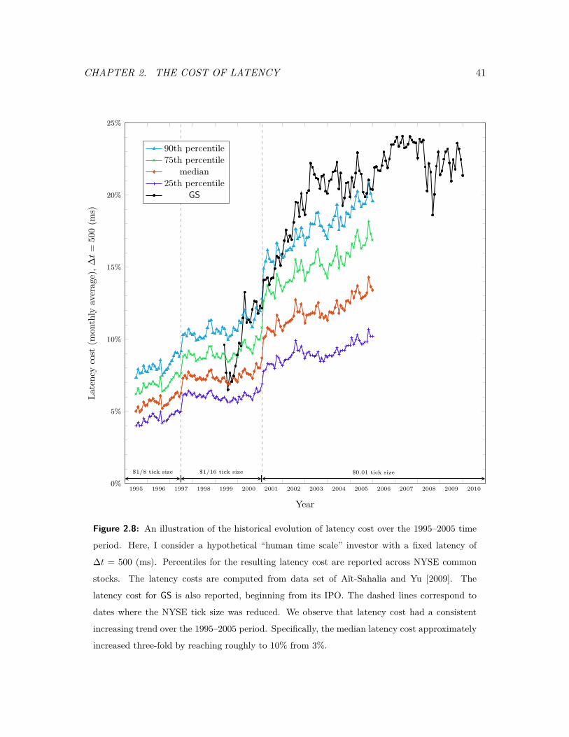
CHAPTER 2. THE COST OF LATENCY 41
1995 1996 1997 1998 1999 2000 2001 2002 2003 2004 2005 2006 2007 2008 2009 20100%
5%
10%
15%
20%
25%
$1/8 tick size $1/16 tick size $0.01 tick size
Year
Late
ncy
cost
(mon
thly
aver
age)
,∆t
=50
0(m
s)
90th percentile75th percentile
median25th percentile
GS
Figure 2.8: An illustration of the historical evolution of latency cost over the 1995–2005 time
period. Here, I consider a hypothetical “human time scale” investor with a fixed latency of
∆t = 500 (ms). Percentiles for the resulting latency cost are reported across NYSE common
stocks. The latency costs are computed from data set of Aït-Sahalia and Yu [2009]. The
latency cost for GS is also reported, beginning from its IPO. The dashed lines correspond to
dates where the NYSE tick size was reduced. We observe that latency cost had a consistent
increasing trend over the 1995–2005 period. Specifically, the median latency cost approximately
increased three-fold by reaching roughly to 10% from 3%.
CHAPTER 2. THE COST OF LATENCY 42
2.5.3. Historical Evolution of Implied Latency
An alternative perspective on the historical importance of latency comes from considering a
hypothetical investor with a target level for the cost of latency, relative to the overall cost-
of-immediacy. The representative trader maintains this target over time through continual
technological upgrades to lower levels of latency. I determine the requisite level of latency
for such a trader, over time and across the aggregate market. In other words, fixing the
latency cost percentage LC to the target level, we can solve the asymptotic approximation
(2.12) for the level of latency required at each time to achieve latency cost LC. I call this
the implied latency.
Figure 2.9 illustrates the implied latency values over the 1995–2005 period assuming
that the target level LC = 10% of overall transaction costs result from latency. We observe
that the median implied latency decreased by approximately two orders of magnitude over
this time frame. The 90th percentile of U.S. equities, for example, went from an implied
latency on the scale of seconds to an implied latency on the scale of tens of milliseconds.
2.5.4. Empirical Importance of Latency
My model captures the cost of latency due to a lack of contemporaneous information.
Figure 2.8 suggests that, when my model is calibrated to the topmost quartile of U.S.
equities, a investor with latency on the human time scale faces a latency cost of at 15% to
25%. In order to assess the significance of this, we can compare it to other trading costs.
Suppose we normalize the cost of immediacy to $0.01, which is the typical bid-offer spread
for a liquid U.S. equity. Then, my model suggests that the benefit of reducing latency
from a human time scale of 500 ms to an ultra low latency time scale of less than 1 ms is
approximately $0.0015–$0.0025 per share traded.
While this might seem very small as an absolute number, note that is of the same
order of magnitude as other trading costs faced by the most cost efficient institutional
investors. For example, a hedge fund would pay an average commission of $0.0007 per
share for market access.14 Furthermore, investors may pay an SEC fee of $0.0005 per share14“U.S. Equity Trading: Low Touch Trends,” TABB Group, July 2010.
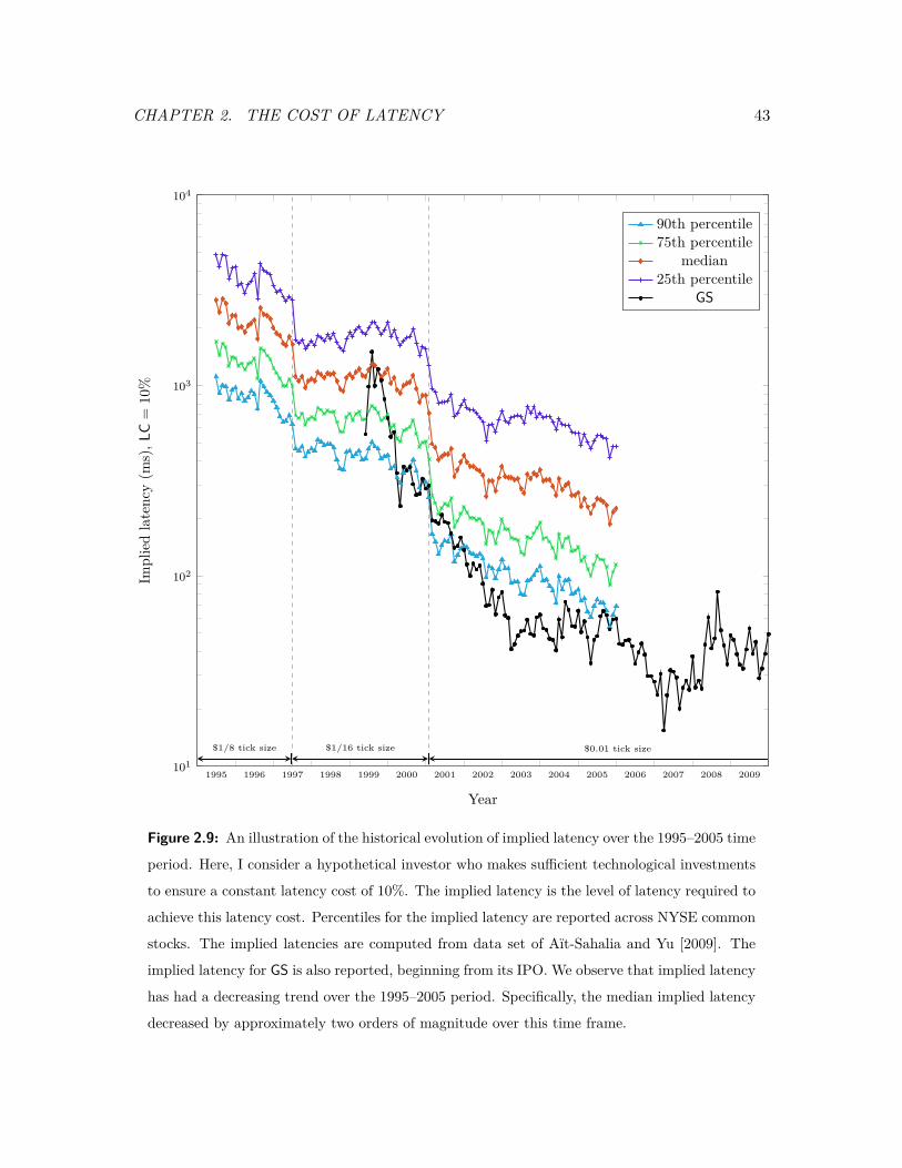
CHAPTER 2. THE COST OF LATENCY 43
1995 1996 1997 1998 1999 2000 2001 2002 2003 2004 2005 2006 2007 2008 2009101
102
103
104
$1/8 tick size $1/16 tick size $0.01 tick size
Year
Impl
ied
late
ncy
(ms)
,LC
=10
%
90th percentile75th percentile
median25th percentile
GS
Figure 2.9: An illustration of the historical evolution of implied latency over the 1995–2005 time
period. Here, I consider a hypothetical investor who makes sufficient technological investments
to ensure a constant latency cost of 10%. The implied latency is the level of latency required to
achieve this latency cost. Percentiles for the implied latency are reported across NYSE common
stocks. The implied latencies are computed from data set of Aït-Sahalia and Yu [2009]. The
implied latency for GS is also reported, beginning from its IPO. We observe that implied latency
has had a decreasing trend over the 1995–2005 period. Specifically, the median implied latency
decreased by approximately two orders of magnitude over this time frame.
CHAPTER 2. THE COST OF LATENCY 44
traded,15 and exchange fees or rebates of $0.0020–$0.0030 per share traded. To the extent
that a sophisticated institutional investor is cost sensitive and wishes to optimize these
other execution costs, they should also be concerned with latency. This isn’t to suggest
that latency cost is important to all investors. A typical retail investor, for example, may
pay a brokerage fee that is up to $0.10 per share traded.16 For this latter type of investor,
the cost of latency as described here is not a significant component of overall trading costs.
Alternatively, we can compare the $0.0015–$0.0025 per share traded latency cost to
the rents extracted by agents that have made the required technological investments to
trade on an ultra low latency time scale. For example, providers of automated algorithmic
trade execution services charge an average commission of $0.0033 per share traded for their
execution services, which leverage sophisticated low latency technological infrastructure.17
Note that this cost is comparable to the latency cost. Another class of agents with ultra
low latency trading capabilities are high frequency traders. Reported net profit numbers
for high frequency traders are in the range of $0.0010–$0.0020 per share traded.18 This is
of the same order of magnitude as the latency cost.
2.6. Conclusion and Future Directions
This chapter provides a model to quantify the cost of latency on transaction costs. I
consider a stylized execution problem, where a trader must sell an atomic unit of stock over
a fixed time horizon. I consider this model in the absence of latency as a benchmark, and15As of January 21, 2011, the SEC fee is a fraction $0.0000192 of the proceeds of an equity sale. If we
assume a typical stock price of $50, this is approximately $0.0010 per share sold. Amortizing this cost
equally between buys and sells results in $0.0005 per share traded.16For example, at the time of writing, the brokerage firm E-TRADE charges $10 per trade. Assuming a
typical trade of 100 shares, this cost is $0.10 per share traded.17“U.S. Equity Trading: Low Touch Trends,” TABB Group, July 2010. Note that some institutional
investors pay significantly larger commissions for trade execution in order to compensate their brokers for
trading ideas or research services. The commission I quote here is for “non-idea driven” services that relate
purely to trade execution using the algorithms and technological platform of the broker.18“Tradeworx, Inc. Public Commentary on SEC Market Structure Concept Release,” Tradeworx, Inc.,
April 2010.
CHAPTER 2. THE COST OF LATENCY 45
I incorporate latency by not allowing the trader to continuously participate in the market.
Orders submitted by the trader reach the market with a fixed latency, and the trader is
forced to deviate from the benchmark policy in order to take into account the uncertainty
introduced by this delay. I quantify the cost of latency as the normalized difference in
expected payoffs between this model and the stylized model without latency.
Since the latency values observed in modern electronic markets are on the order of mil-
liseconds, I provide an asymptotic analysis for the low latency regime, in which I obtain an
explicit closed-form solution. In order to compute this asymptotic latency cost empirically,
I only need to estimate the volatility and the average bid-offer spread of the stock. This is
an elegant and practical result as data sets and estimation procedures for these quantities
are readily abundant in the literature. Indeed, using an existing data set, I show that the
cost of latency incurred by trading on a human time scale (500 ms) increased three-fold over
the 1995–2005 time-frame. In addition, using the alternative approach of keeping a fixed
level of latency cost through continuous technological improvements, I compute the various
percentiles of the implied latency over this time frame. Using the same data set, I observe
that the median implied latency decreased by approximately two orders of magnitude.
My empirical analysis can also be utilized to compare the magnitude of latency cost to
other trading costs incurred by institutional investors. My results suggest that the difference
in payoff between trading with a human time scale (500 ms) and an automated trading
platform with ultra low latency (1 ms) is approximately of the same order of magnitude as
other trading costs faced by institutional investors. This observation certainly underlines
the significance of latency for such investors. In conclusion, my model is the first theoretical
approach in the literature to concretely quantify the impact of latency on the optimal order
submission policy and its resulting cost to the trader.
There are a number of interesting future directions for research. First, as discussed in
Section 2.4.4, there are a number of tractable extensions to the present model that can be
analyzed. One particularly interesting case would be where the bid price process is a jump
process. Here, my suspicion is that the cost of latency would decrease. This is because, even
in the absence of any latency, the trader cannot adjust his limit prices ahead of a jump.
More generally, in the introduction, I identified a number of broad themes to the costs

CHAPTER 2. THE COST OF LATENCY 46
that arise from latency. The model I have presented captures mainly costs due to a lack of
contemporaneous decision making. It does not capture the latency costs due to strategic
effects (i.e., comparative advantage/disadvantage relative to other investors) or due to time
priority rules. These remain important questions for future research.
CHAPTER 3. LINEAR REBALANCING RULES 47
Chapter 3
Dynamic Portfolio Choice with Linear
Rebalancing Rules
3.1. Introduction
Dynamic portfolio optimization has been a central and essential objective for institutional
investors in active asset management. Real world portfolio allocation problems of practical
interest have a number of common features:
• Return predicability. At the heart of active portfolio management is the fact that a
manager will seek to predict future asset returns [Grinold and Kahn, 1999]. Such pre-
dictions are not limited to simple unconditional estimates of expected future returns.
A typical asset manager will make predictions on short- and long-term expected re-
turns using complex models, for example, including return predicting factors such as
market capitalization, book-to-market ratio, lagged returns, dividend yields, gross in-
dustrial production, and other security specific or macroeconomic variables [see, e.g.,
Chen et al., 1986; Fama and French, 1996; Goetzmann and Jorion, 1993].
• Transaction costs. Trading costs in dynamic portfolio management can arise from
sources ranging from the bid-offer spread or execution commissions, to price impact,
where the manager’s own trading affects the subsequent evolution of prices. The effi-
cient management of such costs is an important issue broadly, but becomes especially
CHAPTER 3. LINEAR REBALANCING RULES 48
crucial in the setting of optimal execution. This particular class of portfolio optimiza-
tion problems seeks to optimally liquidate a given portfolio over a fixed time horizon
[Bertsimas and Lo, 1998; Almgren and Chriss, 2000].
• Portfolio or trade constraints. Often times managers cannot make arbitrary invest-
ment decisions, but rather face exogenous constraints on their trades or their resulting
portfolio. Examples of this include short-sale constraints, leverage constraints, or re-
strictions requiring market neutrality (or specific industry neutrality).
• Risk aversion. Portfolio managers seek to control the risk of their portfolios. In
practical settings, risk aversion is not accomplished by the specification of an abstract
utility function. Rather, managers specify limits or penalties for multiple summary
statistics that capture aspects of portfolio risk which are easy to interpret and are
known to be important. For example, a manager may both be interested in the risk of
the portfolio value changing over various intervals of time, including for example, both
short intervals (e.g., daily or weekly risk), as well as risk associated with the terminal
value of the portfolio. Such single period risk can be measured a number of ways
(e.g., variance, value-at-risk). A manager might further be interested in multiperiod
measures of portfolio risk, for example, the maximum drawdown of the portfolio.
Significantly complicating the analysis of portfolio choice is that the underlying problem
is multiperiod. Here, in general, the decision made by a manager at a given instant of time
might depend on all information realized up to that point. Traditional approaches to mul-
tiperiod portfolio choice, dating back at least to the work of Merton [1971], have focussed
on the analytically determining the optimal dynamic policy. While this work has brought
forth important structural insights, it is fundamentally quite restrictive: exact analytical
solutions require very specific assumptions investor objectives and market dynamics. These
assumptions cannot accommodate flexibility in, for example, the return generating pro-
cess, trading frictions, and constraints, and are often practically unrealistic. Absent such
restrictive assumptions, analytical solutions are not possible. Motivated by this, much of
the subsequent academic literature on portfolio choice seeks to develop modeling assump-
tions that allow for analytical solutions, however the resulting formulations are often not
CHAPTER 3. LINEAR REBALANCING RULES 49
representative of real world problems of practical interest. Further, because of the ‘curse-of-
dimensionality’, exact numerical solutions are often intractable as well in cases of practical
interest, where the universe of tradeable assets is large.
In search of tractable alternatives, many practitioners eschew multiperiod formulations.
Instead, they consider portfolio choice problems in a myopic, single period setting, even
when underlying application is clearly multiperiod [e.g., Grinold and Kahn, 1999]. Another
tractable possibility is to consider portfolio choice problems that are multiperiod, but with-
out the possibility of recourse. Here, a fixed set of deterministic decisions for the entire
time horizon are made at the initial time. Both single period and deterministic portfolio
choice formulations are quite flexible, and can accommodate many of the features described
above. They are typically applied in a quasi-dynamic fashion through the method of model
predictive control. Here, at each time period, the simplified single period or deterministic
portfolio choice problem is resolved based on the latest available information. In general,
such methods are heuristics; in order to achieve tractability, they neglect the explicit con-
sideration of the possibility of future recourse. Hence, these methods may be significantly
suboptimal.
A second tractable alternative is the formulation of portfolio choice problems as a linear
quadratic control [e.g., Hora, 2006; Garleanu and Pedersen, 2012]. Since at least the 1950’s,
linear quadratic control problems have been an important class of tractable multiperiod
optimal control problems. In the setting of portfolio choice, if the return dynamics are linear
and the transaction costs and risk aversion penalties decomposed into per period quadratic
functions, and positions and trading decision are unconstrained, then these methods apply.
However, there are many important problem cases that simply do not fall into the linear
quadratic framework.
In this chapter, my central innovation is to propose a framework for multiperiod port-
folio optimization, which admits a broad class of problems including many with features
as described earlier. My formulation maintains tractability by restricting the problem to
determining the best policy out of a restricted class of linear rebalancing policies. Such
policies allow planning for future recourse, but only of a form that can be parsimoniously
parameterized in a specific affine fashion. In particular, the contributions of this chapter
CHAPTER 3. LINEAR REBALANCING RULES 50
are as follows:
1. I define a flexible, general setting for portfolio optimization. My setting allows for
very general dynamics of asset prices, which an arbitrary dependence on a history of
‘return-predictive factors’. I allow for any convex constraints on trades and positions.
Finally, the objective is allowed to be an arbitrary concave function of the sample
path of positions. My framework admits, for example, many complex models for
transaction costs or risk aversion.
2. My portfolio optimization problem is computationally tractable. In my setting, deter-
mining the optimal linear rebalancing policy is a convex program. Convexity guar-
antees that the globally optimal policy can be tractably found in general. This is in
contrast to non-convex portfolio choice parametrizations [e.g., Brandt et al., 2009a],
where only local optimality can be guaranteed.
In my case, numerical solutions can be obtained via, for example, sample average ap-
proximation or stochastic approximation methods [see, e.g., Shapiro, 2003; Nemirovski
et al., 2009]. These methods can be applied in a data-driven fashion, with access only
to simulated trajectories and without an explicit model of system dynamics. In a
number of instances where the factor and return dynamics are driven by Gaussian
uncertainty, I illustrate that my portfolio optimization problem can be reduced to a
standard form of convex optimization program, such as a quadratic program or a sec-
ond order cone program. In such cases, the problem can be solved with off-the-shelf
commercial optimization solvers.
3. My class of linear rebalancing policies subsumes many common heuristic portfolio
policies. Both single period and deterministic policies are special cases of linear re-
balancing polices, however linear rebalancing polices are a broader class. Hence, the
optimal linear rebalancing policy will outperform policies from these more restricted
classes. Further, my method can also be applied in the context of model predictive con-
trol. Also, portfolio optimization problems that can be formulated as linear quadratic
control also fit in my setting, and their optimal policies are linear rebalancing rules.
CHAPTER 3. LINEAR REBALANCING RULES 51
4. I demonstrate the practical benefits of my method in an optimal execution example.
I consider an optimal execution problem where an investor seeks to liquidate a posi-
tion In order to highlight the performance gain using linear decision rules, I use the
discrete-time linear quadratic control formulation of Garleanu and Pedersen [2012].
However, I further introduce linear inequality constraints that allow the trading de-
cisions to only be sales; such sale-only constraints are common in agency algorithmic
trading. I demonstrate that the best linear policy performs better than the best de-
terministic policy, model predictive control and a projected version of the optimal
policy proposed by Garleanu and Pedersen [2012]. Further, the performance of the
best linear policy is shown to be near optimal, by comparison to upper bounds on
optimal policy performance computed for the same problem.
The balance of this chapter is organized as follows: In Section 4.1.1, I review the related
literature. In Section 4.2, I present the abstract form of a dynamic portfolio choice model
and provide various specific problems that satisfy the assumptions of the abstract model.
I formally describe the class of linear decision rules in Section 3.3 and discuss solution
techniques in order to find the optimal parameters of the linear policy. In Section 3.4, I
provide efficient and exact formulations of dynamic portfolio choice models with Gaussian
uncertainty using linear decision models while incorporating linear equality and inequality
constraints, proportional and nonlinear transaction costs and a measure of terminal wealth
risk. In Section 3.5, I apply my methodology in an optimal execution problem and evaluate
the performance of the best linear policy. Finally, in Section 3.6 I conclude and discuss
some future directions.
3.1.1. Related Literature
My chapter is related to two different strands of literature: the literature of dynamic port-
folio choice with return predictability and transaction costs, and the literature on the use
of linear decision rules in the optimal control problems.
First, I consider the literature on dynamic portfolio choice. This vast body of work
begins choice starts with the seminal chapter of Merton [1971]. Following this chapter,
there has been a significant literature aiming to incorporate the impact of various frictions
CHAPTER 3. LINEAR REBALANCING RULES 52
such as transaction costs on the optimal portfolio choice. For a survey on this literature,
see Cvitanic [2001]. The work of Constantinides [1986] is an early example that studies
the impact of proportional transaction costs on the optimal investment decision and the
liquidity premium in the context of CAPM. Davis and Norman [1990], Dumas and Luciano
[1991a], and Shreve and Soner [1994] provide the exact solution for the optimal investment
and consumption decision by formally characterizing the trade and no-trade regions. One
drawback of these papers is that the optimal solution is only computed in the case of a
single stock and bond. Liu [2004] extends these results to multiple assets with fixed and
proportional transaction costs in the case of uncorrelated asset prices. Detemple et al.
[2003] develop a simulation-based methodology for optimal portfolio choice in the presence
of return predictability.
There is also a significant literature on portfolio optimization that incorporates return
predictability [see, e.g., Campbell and Viceira, 2002]. My chapter is related to the liter-
ature that incorporates both return predictability with transaction costs. Balduzzi and
Lynch [1999] and Lynch and Balduzzi [2000] illustrate the impact of return predictability
and transaction costs on the utility costs and the optimal rebalancing rule by discretizing
the state space of the dynamic program. With a similar state space discretization, Lynch
and Tan [2010] model the dynamic portfolio decision with multiple risky assets under re-
turn predictability and transaction costs and provide numerical experiments with two risky
assets. One significant issue with this line of work is that discretization suffers from the
curse-of-dimensionality: the computational effort to determine an optimal policy scales ex-
ponentially with the dimension of the state space. When there are more than a few assets
or return predicting factors, discretization cannot be applied.
Much of the aforementioned literature seeks to find the best rebalancing policy out of
the universe of all possible rebalancing policies. As discussed earlier, this leads to highly
restrictive modeling primitives. On the other hand, my work is in the spirit of Brandt et
al. [2009a], allow for broader modeling flexibility at the expense of considering a restricted
class of rebalancing policies. The parameterize the rebalancing rule as a function of secu-
rity characteristics and estimates the parameters of the rule from empirical data without
modeling the distribution of the returns and the return predicting factors. Even though my
CHAPTER 3. LINEAR REBALANCING RULES 53
approach is also a linear parametrization of return predicting factors, there are fundamental
differences between my approach and that of Brandt et al. [2009a]. First, the class of linear
polices I consider is much larger than the specific linear functional form in Brandt et al.
[2009a]. In my approach the parameters are time-varying and cross-sectionally different for
each security. Second, the extensions provided in Brandt et al. [2009a] for imposing posi-
tivity constraints and transaction costs are ad-hoc and cannot be generalized to arbitrary
convex constraints or transaction cost functions. Finally, the objective function of Brandt
et al. [2009a] is a non-convex function of the policy parameters. Hence, it is not possible,
in general to obtain the globally optimal set of parameters. My setting, on the other hand,
is convex, and hence globally optimal policies can be determined efficiently.
Garleanu and Pedersen [2012] achieve a closed-form solution for a model with linear
dynamics in return predictors and quadratic function for transaction costs and quadratic
penalty term for risk. However, the analytic solution is highly sensitive to the quadratic cost
structure with linear dynamics [see, e.g., Bertsekas, 2000]. This special case cannot handle
any inequality constraints on portfolio positions, non-quadratic transactions costs, or more
complicated risk considerations. On the other hand, my approach can be implemented
efficiently in these realistic scenarios and provides more flexibility in the objective function
of the investor and the constraints that the investor faces. Boyd et al. [2012] consider
an alternative generalization of the linear-quadratic case, using ideas from approximate
dynamic programming. Glasserman and Xu [2011] develop a linear-quadratic formulation
for portfolio optimization that offers robustness to modeling errors or mis-specifications.
Second, there is also a literature on the use of linear decision rules in optimal control
problems. This approximation technique has attracted considerable interest recently in
robust and two-stage adaptive optimization context [see, e.g., Ben-Tal et al., 2004, 2005;
Chen et al., 2007, 2008; Bertsimas et al., 2010; Bertsimas and Goyal, 2011]. Shapiro and
Nemirovski [2005] illustrate that linear decision rules can reduce the complexity of multi-
stage stochastic programming problems. Kuhn et al. [2009] proposes an efficient method to
estimate the loss of optimality incurred by linear decision rule approximation.
In this strand of literature, I believe the closest works to the methodology described in
my chapter are Calafiore [2009] and Skaf and Boyd [2010]. Both of these papers use linear
CHAPTER 3. LINEAR REBALANCING RULES 54
decision rules to address dynamic portfolio choice problems with proportional transaction
costs without return predictability. Calafiore [2009] compute lower and upper bounds on
the expected transaction costs and solves two convex optimization problems to get upper
and lower bounds on the optimal value of the simplified dynamic optimization program with
linear decision rules. On the other hand, Skaf and Boyd [2010] study the dynamic portfolio
choice problem as an application to their general methodology of using affine controllers
on convex stochastic programs. They first linearize the dynamics of the wealth process
and then solve the resulting convex optimization via sampling techniques. The foremost
difference between my approach and these papers is the modeling of return predictability.
Hence, the optimal rebalancing rule in my model is a linear function of the predicting
factors. Furthermore, I derive exact reductions to deterministic convex programs in the
cases of proportional and nonlinear transaction costs.
3.2. Dynamic Portfolio Choice with Return Predictability and
Transaction Costs
I consider a dynamic portfolio choice problem with allowing general models for the pre-
dictability of security returns and for trading frictions. The number of investable securities
is N , time is discrete and indexed by t = 1, . . . , T , where T is the investment horizon. Each
security i has a price change1 of ri,t+1 from time t to t+ 1.
I collect these price changes in the return vector rt+1 , (r1,t+1, . . . , rN,t+1). I assume
that the investor has a predictive model of future security returns, and that these predic-
tions are made through a set of set of K return-predictive factors. These factors could be
security specific characteristics such as the market capitalization of the stock, the book-to-
market ratio of the stock, the lagged twelve month return of the stock [see, e.g., Fama and
French, 1996; Goetzmann and Jorion, 1993]. Alternatively, they could be macroeconomic
signals that affect the return of each security, such as inflation, treasury bill rate, industrial1I choose to describe the evolution of asset prices in my framework in terms of absolute price changes,
and I will also refer to these as (absolute) returns. Note that this is without loss of generality: since the
return dynamics specified by Assumption 1 allow for an arbitrary dependence on history, my framework also
admits, for example, models which describe the rate of return of each security.
CHAPTER 3. LINEAR REBALANCING RULES 55
production [see, e.g., Chen et al., 1986]. Denote by ft ∈ RK the vector of factor values at
time t. I assume very general dynamics, possibly nonlinear and with a general dependence
on history, for the evolution of returns and factors.
Assumption 1 (General return and factor dynamics). Over a complete filtered probability space
given by (Ω,F , Ftt≥0 ,P), I assume that factors and returns evolve according to
ft+1 = Gt+1(ft, . . . , f1, εt+1), rt+1 = Ht+1(ft, εt+1),
for each time t. Here, Gt+1(·) and Ht+1(·) are known functions that describe the evolution
of the factors and returns in terms of the history of factor values and the exogenous, i.i.d.
disturbances εt+1. I assume that the filtration F , Ftt≥0 is the natural filtration generated
by the exogenous noise terms εt.
Let xi,t denote the number of shares that the investor holds in ith security over the
time period t. I collect the portfolio holdings across all securities at time t in the vector
xt , (x1,t, . . . , xN,t), and I denote the fixed initial portfolio of the investor by x0. Similarly,
let the trade vector ut , (u1,t, . . . , uN,t) denote the amount of shares that the investor wants
to trade at the beginning of the tth period, when he inherits the portfolio xt−1 from the
prior period and observes the latest realization of factor values ft. Consequently, we have
the following linear dynamics for my position and trade vector: xt = xt−1 + ut, for each t.
Let the entire sample path of portfolio positions, factor realizations, and security re-
turns be denoted by x , (x1, . . . , xT ), , (f1, . . . , fT), and r , (r2, . . . , rT+1), respectively.
Similarly, the sample path of trades over time is denoted by u = (u1, . . . , uT ). I make the
following assumption on feasible sample paths of trades:
Assumption 2 (Convex trading constraints). The sample path of trades u are restricted to
the non-empty, closed, and convex set U ⊆ RN × . . .× RN .
The investor’s trading decisions are determined by a policy π that selects a sample path
of trades u in U for each realization of r and f . I let U be the set of all policies. I assume that
the investor’s trading decisions are non-anticipating in that the trade vector ut in period t
depends only on what is known at the beginning of period t. Formally, I require policies to
CHAPTER 3. LINEAR REBALANCING RULES 56
be adapted to the filtration F, such that a policy’s selection of the trade vector ut at time
t must be measurable with respect to Ft. Let UF be the set of all non-anticipating policies.
The objective of the investor is to select a policy π ∈ UF that maximizes the expected
value of a total reward or payoff function p(·). Formally, I consider the following optimiza-
tion problem for the investor,
(3.1) supπ∈UF
Eπ[p(x, f , r)],
where the real-valued reward function p(·) is a function of the entire sample path of portfolio
positions, x, the factor realization, f , and security returns r. For example, p(·) may have
the form
(3.2) p(x, f , r) ,W (x, r)− TC(u)− RA(x, f , r).
Here, W denotes the terminal wealth (total trading gains ignoring of transaction costs),
i.e.,
(3.3) W (x, r) ,W0 +T∑t=1
x>t rt+1,
where W0 is the initial wealth. TC(·) captures the transaction costs associated with a set
of trading decisions, and RA(·) is the penalty term that incorporates risk aversion.
I make the following assumption about my objective function:
Assumption 3 (Concave objective function). Given an arbitrary, fixed sample paths of factor
realizations f and security returns r, assume that the reward function p(x, f , r) is a concave
function of the sequence of positions x.
If p(·) has the specified form in (3.2), then Assumption 3 will be satisfied when the
transaction cost term TC(·) is a convex function of trades and the risk aversion term RA(·)
is a convex function of portfolio positions.
3.2.1. Examples
In this chapter, I consider dynamic portfolio choice models that satisfy Assumptions 1–3.
In order to illustrate the generality of this setting, I will now provide a number of specific
examples that satisfy these assumptions.
CHAPTER 3. LINEAR REBALANCING RULES 57
Example 1 (Garleanu and Pedersen 2012). This model has the following dynamics, where
returns are driven by mean-reverting factors, that fit into my general framework:
ft+1 = (I − Φ) ft + ε(1)t+1, rt+1 = µt +Bft + ε
(2)t+1,
for each time t ≥ 0. Here, µt is the deterministic ‘fair return’, e.g., derived from the
CAPM, while B is a matrix of constant factor loadings. The factor process ft is a vector
mean-reverting process, with Φ a matrix of mean reversion coefficients for the factors. It is
assumed that the i.i.d. disturbances εt+1 , (ε(1)t+1, ε
(2)t+1) are zero-mean with covariance given
by Var(ε(1)t+1) = Ψ and Var(ε(2)
t+1) = Σ.
Trading is costly, and the transaction cost to execute ut = xt − xt−1 shares is given by
TCt(ut) , 12utΛut, where Λ ∈ RN×N is a positive semi-definite matrix that measures the
level of trading costs. There are no trading constraints (i.e., U , RN×T ). The investor’s
objective function is to choose a trading strategy to maximize discounted future expected
excess return, while accounting for transaction costs and adding a per-period penalty for
risk, i.e.,
(3.4) maximizeπ∈UF
Eπ[T∑t=1
(x>t Bft − TCt(ut)− RAt(xt)
)].
where RAt(xt) , γ2x>t Σxt is a per-period risk aversion penalty, with γ being a coefficient
of risk aversion. Garleanu and Pedersen [2012] suggest this objective function for an in-
vestor who is compensated based on his performance relative to a benchmark. Each x>t Bftterm measures the excess return over the benchmark, while each RAt(xt) term measures the
variance of the tracking error relative to the benchmark.2
The problem (3.4) clearly falls into my framework. The objective function is similar to
that of (3.2) with the minor variation expected excess return rather than expected wealth
is considered. Further, (3.4) has the further special property that total transaction costs
and penalty for risk aversion decompose over time:
RA(x, f , r) ,N∑t=1
RAt(xt), TC(u) ,N∑t=1
TCt(ut).
2See Garleanu and Pedersen [2012] for other interpretations.
CHAPTER 3. LINEAR REBALANCING RULES 58
Note that this problem can be handled easily using the classical theory from the linear-
quadratic control (LQC) literature [see, e.g., Bertsekas, 2000]. This theory provides analyt-
ical characterization of optimal solution, for example, that the value function at any time t
is quadratic function the state (xt, ft), and that the optimal trade at each time is an affine
function of the state. Moreover, efficient computational procedures are available to solve
for the optimal policy.
On the other hand, the tractability of this model rests critically on three key require-
ments:
• The state variables (xt, ft) at each time t must evolve as linear functions of the control
ut and the i.i.d. disturbances εt (i.e., linear dynamics).
• Each control decision ut is unconstrained.
• The objective function must decompose across time into a positive definite quadratic
function of (xt, ut) at each time t.
These requirements are not satisfied by many real world examples, which may involve
portfolio position or trade constraints, different forms of transaction costs and risk measures,
and more complicated return dynamics. In the following examples, I will provide concrete
examples of many such cases that do not admit optimal solutions via the LQC methodology,
but remain within my framework.
Example 2 (Portfolio or trade constraints). In practice, a common constraint in constructing
equity portfolios is the short-sale restriction. Most of the mutual funds are enforced not to
have any short positions by law. This requires the portfolio optimization problem to include
the linear constraint
xt = x0 +t∑
s=1ut ≥ 0,
for each t. This is clearly a convex constraint on the set of feasible trade sequence u.
I observe a similar restriction when an execution desk needs to sell or buy a large portfolio
on behalf of an investor. Due to the regulatory rules in agency trading, the execution desk
is only allowed to sell or buy during the trading horizon. In the ‘pure-sell’ scenario, the
CHAPTER 3. LINEAR REBALANCING RULES 59
execution desk needs to impose the negativity constraint
ut ≤ 0,
for each time t.
Simple linear constraints such as these fit easily in my framework, but cannot be ad-
dressed via traditional LQC methods.
Example 3 (Non-quadratic transaction costs). In practice, many trading costs such as the
bid-ask spread, broker commissions, and exchange fees are intrinsically proportional to the
trade size. Letting χi be the the proportional transaction cost rate (an aggregate sum of
bid-ask cost and commission fees, for example) for trading security i, the investor will incur
a total cost of
TC(u) ,T∑t=1
N∑i=1
χi|ui,t|.
The proportional transaction costs are a classical cost structure that is well studied in the
literature [see, e.g., Constantinides, 1986].
Furthermore, other trading costs occur due to disadvantageous transaction price caused
by the price impact of the trade. The management of the trading costs due to price impact
has recently attracted considerable interest [see, e.g., Obizhaeva and Wang, 2005; Almgren
and Chriss, 2000]). Many models of transaction costs due to price impact imply a nonlinear
relationship between trade size and the resulting transaction cost, for example
TC(u) ,T∑t=1
N∑i=1
χi|ui,t|β.
Here, β ≥ 13 and χi is a security specific proportionality constant.
In general, when the trade size is small relative to the total traded volume, proportional
costs will dominate. On the other hand, when the trade size is large, costs due to price
impact will dominate. Hence, both of these types of trading are important. However, the
LQC framework of Example 1 only allows quadratic transaction costs (i.e., β = 2).
Example 4 (Terminal wealth risk). The objective function of Example 1 includes a term to
penalize excessive risk. In particular, the per-period quadratic penalty, x>t Σxt, is used, in3Gatheral [2010] notes that β = 3
2 is a typical assumption in practice.
CHAPTER 3. LINEAR REBALANCING RULES 60
order to satisfy the requirements of the LQC model. However, penalizing additively risk in
a per-period fashion is nonstandard. Such a risk penalty does not correspond to traditional
forms of investor risk preferences, e.g., maximizing the utility of terminal wealth, and the
economic meaning of such a penalty is not clear. An investor is typically more interested
in the risk associated with the terminal wealth, rather than a sum of per-period penalties.
In order to account for terminal wealth risk, let ρ : R → R be a real-valued convex
function meant to penalize for excessive risk of terminal wealth (e.g., ρ(w) = 12w
2 for a
quadratic penalty) and consider the optimization problem
(3.5) maximizeπ∈UF
Eπ[W (x, r)− TC(u)− γρ(W (x, r))
],
where γ > 0 is a risk-proportionality constant.
It is not difficult to see that the objective in (3.5) satisfies Assumption 3 and hence
fits into my model. However, even when the risk penalty function ρ(·) is quadratic, (3.5)
does not admit a tractable LQC solution, since the quadratic objective does not decompose
across time.
Example 5 (Maximum drawdown risk). In addition to the terminal measures of risk described
in Example 4, an investor might also be interested controlling intertemporal measures of risk
defined over the entire time trajectory. For example, a fund manager might be sensitive to
a string of successive losses that may lead to the withdrawal of assets under management.
One way to limit such losses is to control the maximum drawdown, defined as the worst loss
of the portfolio between any two points of time during the investment horizon 4. Formally,
MD(x, r) , max1≤t1≤t2≤T
− t2∑t=t1
x>t rt+1, 0
.It is easy to see that the maximum drawdown is a convex function of x. Hence, the portfolio
optimization problem
(3.6) maximizeπ∈UF
Eπ [W (x, r)− TC(u)− γMD(x, r)],
where γ ≥ 0 is a constant controlling tradeoff between wealth and the maximum drawdown
penalty, satisfies Assumption 3. Moreover, standard convex optimization theory yields that4For example, see Grossman and Zhou [1993] for an earlier example.
CHAPTER 3. LINEAR REBALANCING RULES 61
the problem (3.6) is equivalent to solving the constrained problem
(3.7)maximize
π∈UFEπ [W (x, r)− TC(u)]
subject to Eπ [MD(x, r)] ≤ C,
where C (which depends on the choice of γ) is a limit on the allowed expected maximum
drawdown.
Example 6 (Complex dynamics). I can also generalize the dynamics of Example 1. Consider
factor and return dynamics given by
ft+1 = (I − Φ) ft + ε(1)t+1, rt+1 = µt + (B + ξt+1)ft + ε
(2)t+1,
for each time t ≥ 0. Here, each ξt+1 ∈ RN×K is an extra noise term which captures model
uncertainty regarding the factor loadings. I assume that
E [ (B + ξt+1) ft | Ft] = Bft, Var [(B + ξt+1) ft | Ft] = f>t Υft.
With this model, the conditional variance of returns becomes dependent on the factor struc-
ture and is time-varying, i.e., Var[rt+1|Ft] = f>t Υft + Σ. This is consistent with the em-
pirical work of Fama and French [1996], for example. In this setting, the per-period penalty
of risk analogous to that in (3.4) becomes RAt(x, f) = x>t
(f>t Υft + Σ
)xt. The resulting
optimal control problem no longer falls into the LQC framework.
The dynamics and the reward functions considered in these examples satisfy my basic
requirements of Assumptions 1–3. These examples illustrate that in many real-world prob-
lems with complex primitives for return predictability, transaction costs, risk measures and
constraints, the dynamic portfolio choice becomes difficult to solve analytically via LQC
methods.
3.3. Optimal Linear Model
The examples of Section 3.2.1 illustrated a broad range of practically important portfolio
optimization problems. Without special restrictions, such as those imposed in the LQC
framework, the optimal dynamic policy for such a broad set of problems cannot be computed
CHAPTER 3. LINEAR REBALANCING RULES 62
either analytically or computationally. In this section, in order to obtain policies in a
computationally tractable way, I will consider a more modest goal. Instead of finding the
optimal policy amongst all admissible dynamic policies, I will restrict my search to a subset
of policies that are parsimoniously parameterized. That is, instead of solving for a globally
optimal policy, I will instead find an approximately optimal policy by finding the best policy
over the restricted subset of policies.
In order to simplify, I will assume that reward function of the investor’s optimization
(3.1) is a function only of the sample path of portfolio positions x and of factor realizations
f , and does not depend on the security returns r. In other words, I assume that the reward
function takes the form p(x, f). This is without loss of generality — given my general
specification for factors under Assumption 1, we can simply include each security return
as a factor. With this assumption, investor’s trading decisions will, in general, be a non-
anticipating function of the sample path of factor realizations f . However, consider the
following restricted set of policies, linear rebalancing policies, which are obtained by taking
the affine combinations of the factors:
Definition 2 (Linear rebalancing policy). A linear rebalancing policy π is a non-anticipating
policy parameterized by collection of vectors c , ct ∈ RN , 1 ≤ t ≤ T and a collection
of matrices E , Es,t ∈ RN×K , 1 ≤ s ≤ t ≤ T, that generates a sample path of trades
u , (u1, . . . , uT ) according to
(3.8) ut , ct +t∑
s=1Es,tfs,
for each time t = 1, 2, . . . , T .
Define C to be the set of parameters (E, c) such that the resulting sequence of trades u
is contained in the constraint set U , with probability 1, i.e., u is feasible. Denote by L ⊂ UFthe corresponding set of feasible linear policies.
Observe that linear rebalancing allow recourse, albeit in a restricted functional form.
The affine specification (3.8) includes several classes of polices of particular interest as
special cases:
• Deterministic policies. By taking Es,t , 0, for all 1 ≤ s ≤ t ≤ T , it is easy to see
that any deterministic policy is a linear rebalancing policy.
CHAPTER 3. LINEAR REBALANCING RULES 63
• LQC optimal policies. Optimal portfolios for the LQC framework of Example 1 take
the form xt = Γx,txt−1 + Γf,tft, given matrices Γx,t ∈ RN×N , Γf,t ∈ RN×K , for all
1 ≤ t ≤ T , i.e., the optimal portfolio are linear in the previous position and the current
factor values. Equivalently, by induction on t,
xt =(
t∏s=1
Γx,s
)x0 +
t∑s=1
(s−1∏`=1
Γx,`
)Γf,sfs.
Since ut = xt − xt−1, it is clear that the optimal trade ut is a linear function of the
fixed initial position x0, and the factor realizations f1, . . . , ft, and is therefore of the
form (3.8).
• Linear portfolio polices. Brandt et al. [2009a] suggest a class of policies where port-
folios are determined by adjusting a deterministic benchmark portfolio according to
a linear function of a vector of stochastic, time-varying firm characteristics. In my
setting, the firm characteristics would be interpreted as stochastic return predict-
ing factors. An analogous rule would determine the positions at each time t via
xt = xt + Θ>t (ft− ft). Here, ft is the expected factor realization at time t. The policy
is parameterized by xt, the deterministic benchmark portfolio at time t, and the ma-
trix Θt ∈ RN×K , which maps firm characteristics (standardized to be mean zero) to
adjustments to the benchmark portfolio. Such a portfolio rule is clearly of the form
(3.8).
• Policies based on basis functions. Instead of having policies that are directly affine
function of factor realizations, it is also possible to introduce basis functions. One
might consider, for example, ϕ : RK → RD, a collection of D (non-linear) functions
that capture particular features of the factor space that are important for good decision
making. Consider a class of policies of the form
ut , ct +t∑
s=1Es,tϕ(fs).
Such policies belong to the linear rebalancing class, if the factors are augmented
also to include the value of the basis functions. This is easily accommodated in my
framework, given the flexibility of Assumption 1. Similarly, policies which depend on
CHAPTER 3. LINEAR REBALANCING RULES 64
the past security returns (in addition to factor realizations) can be accomodated by
augmenting the factors with past returns.
An alternative to solving the original optimal control problem (3.1) is to consider the
problem
(3.9) supπ∈L
Eπ[p(x, f)],
which restricts to linear rebalancing rules. In general, (3.9) will not yield an optimal control.
The exception is if the optimal control for the problem is indeed a linear rebalancing rule
(e.g., in a LQC problem). However, (3.9) will yield the best possible linear rebalancing rule.
Further, in contrast to the original optimal control problem, (3.9) has the great advantage
of being tractable, as suggested by the following result:
Proposition 1. The optimization problem given by
(3.10)
maximizeE,c
E[p(x, f)]
subject to xt = xt−1 + ut, ∀ 1 ≤ t ≤ T,
ut = ct +t∑
s=1Es,tfs, ∀ 1 ≤ t ≤ T,
(E, c) ∈ C.
is a convex optimization problem, i.e., it involves the maximization of a concave function
subject to convex constraints.
Proof. Note that p(·, f) is concave for a fixed f by Assumption 3, and since x can be written
as an affine transformation of (E, c). Then, for each fixed f , the objective function is concave
in (E, c). Taking an expectation over f preserves this concavity. Finally, the convexity of
the constraint set C follows from the convexity of U , under Assumption 2.
The problem (3.10) is a finite-dimensional, convex optimization problem that will yield
parameters for the optimal linear rebalancing policy. It is also a stochastic optimization
problem, in the sense that the objective is the expectation of a random quantity. In general,
there are a number of effective numerical methods that can been applied to solve such
problems:
CHAPTER 3. LINEAR REBALANCING RULES 65
• Efficient exact formulation. In many cases, with further assumptions on the prob-
lem primitives (the reward function p(·), the dynamics of the factor realizations f ,
and the trading constraint set U), the objective E[p(x, f)] and the constraint set C
of the program (3.10) can be explicitly analytically expressed in terms of the deci-
sion variables (E, c). In some of these cases, the program (3.10) can be transformed
into a standard form of convex optimization program such as a quadratic program
or a second-order cone program. In such cases, off-the-shelf solvers specialized to
these standard forms [e.g., Grant and Boyd, 2011] can be used. Alternatively, generic
methods for constrained convex optimization such as interior point methods [see, e.g.,
Boyd and Vandenberghe, 2004] can be applied to efficiently solve large-scale instances
of (3.10). I will explore this topic further, developing a number of efficient exact
formulations in Section 3.4, and providing a numerical example in Section 3.5.
• Sample average approximation (SAA). In the absence of further structure on the
problem primitives, the program (3.10) can also be solved via Monte Carlo sampling.
Specifically, supposed that f (1), . . . , f (S) are S independent sample paths of factor
realization. The objective and constraints of (3.10) can be replaced with sampled
versions, to obtain
(3.11)
maximizeE,c
1S
S∑`=1
p(x(`), f (`)
)subject to x
(`)t = x
(`)t−1 + u
(`)t , ∀ 1 ≤ t ≤ T, 1 ≤ ` ≤ S,
u(`)t = ct +
t∑s=1
Es,tf(`)s , ∀ 1 ≤ t ≤ T, 1 ≤ ` ≤ S,
u(`) ∈ U, ∀ 1 ≤ ` ≤ S.
The sample average approximation (3.11) can be solved via standard convex optimiza-
tion methods (e.g., interior point methods). Moreover, under appropriate regularity
conditions, convergence of the SAA (3.11) to the original program (3.10) can be es-
tablished as S → ∞, along with guarantees on the rate of convergence [Shapiro,
2003].
• Stochastic approximation. Denote the collection of decision variables in (3.10) by
z , (E, c), and, allowing a minor abuse of notation, define p(z, f) to be the reward
CHAPTER 3. LINEAR REBALANCING RULES 66
when the sample path of factor realizations is given by f and the trading policy
is determined by z. Then, defining h(z) , p(z, f), the problem (3.10) is simply
to maximize h(z) subject to the constraint that z ∈ C. Under suitable technical
conditions, superdifferentials of h and p are related according to ∂h(z) = E[∂zp(z, f)].
Stochastic approximation methods are incremental methods that seek to estimate
ascent directions for h(·) from sampled ascent directions for p(·, f). For example,
given a sequence of i.i.d. sample paths of factor realizations f (1), f (2), . . ., a sequence
of parameter estimates z(1), z(2), . . . can be constructed according to
z(`+1) = ΠC(z(`) + γ`ζ`
),
where ΠC(·) is the projection onto the feasible set C, ζ` ∈ ∂zp(z(`), f (`) ) is a supergradi-
ent, and γ` > 0 is a step-size. Stochastic approximation methods have the advantage
of being incremental and thus requiring minimal memory relative to sample average
approximation, and are routinely applied in large scale convex stochastic optimization
[Nemirovski et al., 2009].
One attractive feature of the sample average approximation and stochastic approxima-
tion approaches is that they can be applied in a data-driven fashion. These methods need
access only to simulated trajectories of factors and returns — they do not need explicit
knowledge of the dynamics in Assumption 1 that drive these processes. Hence, an optimal
linear rebalancing policy can be determined using, for example, historical data to construct
simulated trajectories, without specifying and estimating an explicit functional form for the
factor and return dynamics.
Finally, observe that optimal linear policies can also be applied in concert with model
predictive control (MPC). Here, at each time step t, the program (3.10) is resolved beginning
from time t. This determines the optimal linear rebalancing rule from time t forward,
conditioned on the realized history up to time t. The resulting policy is only used to
determine the trading decision at the then current time t, and (3.10) is subsequently resolved
at each future time period. At the cost of an additional computational burden, the use of
optimal linear policies with MPC subsumes standard MPC approaches, such as resolving a
myopic variation of the portfolio optimization problem (and ignoring the true multiperiod
CHAPTER 3. LINEAR REBALANCING RULES 67
nature) or solving a deterministic variation of the portfolio optimization problem (and
ignoring the possibility of future recourse).
3.4. Efficient Exact Formulations
In this section, I will provide efficient exact formulations of dynamic portfolio choice prob-
lems using the class of linear policies for my feasible set of policies. In particular, I will
consider a number of the examples of dynamic portfolio choice problems discussed in Sec-
tion 3.2.1. These examples include features such as constraints on portfolio holdings, trans-
action costs, and risk measures. In each case, I will demonstrate how the optimization
problem (3.10) can be transformed into a deterministic convex program by explicit analyt-
ical evaluation of the objective function E[p(·, f)] and the constraint set C.
Exact formulations require the evaluation of expectations taken over the sample path of
factor realizations f . In order to do this, I will make the following assumption for the rest
of this section:
Assumption 4 (Gaussian factors). Assume that the sample path f of factor realizations is
jointly Gaussian. In particular, denote by Ft , (f1, . . . , ft)> ∈ RKt the vector of all factors
observed by time t. I assume that Ft ∼ N(θt,Ωt), where θt ∈ RKt is the mean vector and
Ωt ∈ RKt×Kt is the covariance matrix.
With this assumption, the trades of any linear policy will also be jointly normally
distributed, as each such policy is affine transformations of the factors. Formally, let
(3.12) Mt ,[E1,t E2,t . . . Et,t
]∈ RN×Kt
be the matrix of time t policy coefficients, so that the trade vector is given by ut = ct+MtFt.
With this representation, it is easy see that ut ∼ N(ut, Vt), where the mean vector and
covariance matrix are given by
ut , E[ut] = ct +Mtθt, Vt , Var(ut) = MtΩtM>t .(3.13)
Similarly, the portfolio xt at time t is normally distributed. I have that
(3.14) xt = x0 +t∑i=1
ui = x0 +t∑i=1
(ci +
i∑s=1
Es,ifs
)= dt +
t∑s=1
Js,tfs,
CHAPTER 3. LINEAR REBALANCING RULES 68
where dt , x0 +∑ti=1 ci and Js,t ,
∑t`=sEs,`. With this representation, it is easy see that
xt ∼ N(κt, Yt), where
κt , E[xt] = dt + Ptθt, Yt , Var(xt) = PtΩtP>t ,(3.15)
Pt ,[J1,t J2,t . . . Jt,t
].(3.16)
3.4.1. Linear Constraints
I will provide formulations for linear equality or inequality constraints on trades or positions,
in the context of linear rebalancing policies. These type of constraint appear frequently in
portfolio choice due to regulatory reasons such as short sale restriction, liquidation purposes
or diversification needs such as keeping a specific industry exposure under a certain limit.
3.4.1.1. Equality Constraints
Equality constraints appear often in portfolio choice, particularly in portfolio execution
problems when the investor needs to liquidate a certain portfolio (i.e., xT = 0) or construct
a certain target portfolio by the end of the time horizon (i.e., xT = x).
Suppose that for some time t, have a linear equality constraint on the trade vector ut,
of the form Aut = b. Here, A ∈ RM×N and b ∈ RN . This constraint can be written as
(3.17) Act +AMtFt = b.
Under Assumption 4, the left hand side of the (3.17) is normally distributed. Therefore,
for (3.17) to hold almost surely, I must have that the left hand side have mean b and zero
covariance. Thus, I require that
Act = b, AMt = 0.(3.18)
Thus, the linear equality constraint (3.17) on the trade vector ut is equivalent to the linear
equality constraint (3.18) on the policy coefficients (ct,Mt). Linear equality constraints on
the portfolio position xt can be handled similarly.
CHAPTER 3. LINEAR REBALANCING RULES 69
3.4.1.2. Inequality Constraints
Inequality constraints on trades or positions are common as well. One example is a short-sale
constraint, which would require that xt ≥ 0 for all times t. When the factor realizations do
not have bounded support, inequality constraints cannot be enforced almost surely. This is
true in the Gaussian case: there is a chance, however small, that factors may take extreme
values, and if the policy if a linear function of the factors, this may cause an inequality
constraint to be violated.
In order to account for such constraints in a linear rebalancing policy, instead of enforcing
inequality constraints almost surely, we will enforce them at a given level of confidence. For
example, given a vector a ∈ RN and a scalar b, instead of enforcing the linear constraint
a>ut ≤ b, almost surely, we can consider a relaxation where seek to guarantee that it
is violated with small probability. In other words, we can impose the chance constraint
P(a>ut > b) ≤ η, for a small value of the parameter η. The following lemma, whose proof
can be found in the Online Supplement, illustrates that this can be accomplished explicitly:
Lemma 3. Given η ∈ [0, 1/2], a non-zero vector a ∈ RN , and a scalar b, the chance con-
straint P(a>ut > b) ≤ η is equivalent to the constraint
a> (ct +Mtθt)− b+ Φ−1(1− η)∣∣∣∣∣∣Ω1/2
t M>t a∣∣∣∣∣∣
2≤ 0
on the policy coefficients (ct,Mt), where Φ−1(·) is the inverse cumulative normal distribu-
tion.
A similar approach be applied to incorporate linear inequality constraints on the port-
folio position xt with high confidence.
In many situations (e.g., short-sale constraints), it may not be sufficient to enforce an
inequality constraint only probabilistically. In such cases, when a linear rebalancing policy
is applied, the resulting trades can be projected onto the constraint set so as to ensure
that the constraints are always satisfied. When the linear policy is designed, however, it
is helpful to incorporate the desired constraints probabilistically so as to account for their
presence. I will demonstrate this idea in the application in Section 3.5.
CHAPTER 3. LINEAR REBALANCING RULES 70
3.4.2. Transaction Costs
In this section, I will provide efficient exact formulations for the transaction cost functions
discussed in Section 3.2.1, in the context of linear rebalancing policies. In general, once
might consider a total transaction cost of
TC(u) ,T∑t=1
TCt(ut)
for executing the sample path of trades u, where TCt(ut) is the cost of executing the trade
vector ut at time t. As seen in Section 3.2.1, we typically wish to subtract an expected
transaction cost term from investor’s objective. Hence efficient exact formulations for trans-
action costs involve explicit analytical computation of E[TC(u)] =∑Tt=1 E[TCt(ut)], when
each trade vector ut is specified by a linear policy.
Under a linear policy, ut ∼ N(ut, Vt) is distributed as a normal random variable, with
mean and covariance (ut, Vt) specified from the policy (E, c) coefficients through (3.13).
Then, the evaluation of expected transaction costs reduces to the evaluation of the expected
value of the per period transaction cost function TCt(·) for a Gaussian argument. This can
be handled on a case-by-case basis as follows:
• Quadratic transaction costs. In the case of quadratic transaction costs, as seen in Ex-
ample 1, the per period transaction cost function is given by TCt(ut) , 12u>t Λut, where
Λ ∈ RN×N is a positive definite matrix. In this case, E[TCt(ut)] = 12 (utΛut + tr(ΛVt)) .
• Proportional transaction costs. In the case of proportional transaction costs, as
discussed in Example 3, the per period transaction cost function is given by
TCt(ut) ,N∑i=1
χi|ut,i|,
where χi > 0 is a proportionality constant specific to security i. Using the properties
of the folded normal distribution, I obtain
E[TCt(ut)] =N∑i=1
χi
√2Vt,iπ
exp−u2t,i
2Vt,i
+ ut,i
1− 2Φ
(− ut,i√
Vt,i
) ,where Φ(·) is the cumulative distribution function of a standard normal random vari-
able.
CHAPTER 3. LINEAR REBALANCING RULES 71
• Nonlinear transaction costs. In the case of nonlinear transaction costs, as discussed
in Example 3, the per period transaction cost function is given by
TCt(ut) ,N∑i=1
χi|ut,i|β,
where χi > 0 is a proportionality constant specific to security i, and β ≥ 1 is an
exponent capturing the degree of nonlinearity. As in the proportional case, evaluating
the Gaussian expectation explicitly results in
E[TCt(ut)] =N∑i=1
χiΓ(1 + β
2
) (2Vt,i)β2
√π
1F1
(−β2 ; 1
2;−u2t,i
2Vt,i
),
where Γ(·) is the gamma function and 1F1(·) is the confluent hypergeometric function
of the first kind.
3.4.3. Terminal Wealth and Risk Aversion
In many of the portfolio choice examples in Section 3.2.1, an investor wishes to maximize
expected wealth net of transaction costs, subject to a penalty for risk, i.e.,
(3.19) maximizeπ∈UF
Eπ[W (x, r)− TC(u)− RA(x, f , r))
].
Here, W (·) is the terminal wealth associated with a sample path, TC(·) are the transaction
costs, and RA(·) is a penalty for risk aversions. Exact calculation of expected transaction
costs for linear policies were discussed in Section 3.4.2. Here, I will discuss exact calculation
of the expected terminal wealth and the risk aversion penalty.
To begin, note that the terminal wealth depends on realized returns in addition to factor
realizations. Hence, I will make the following assumption:
Assumption 5 (Gaussian returns). As in Example 1, assume that for each time t ≥ 0, returns
evolve according to
(3.20) rt+1 = µt +Bft + ε(2)t+1,
where µt is a deterministic vector, B is a matrix of factor loadings, and ε(2)t are zero-mean
i.i.d. Gaussian disturbances with covariance Σ.
CHAPTER 3. LINEAR REBALANCING RULES 72
Note that the critical assumption I am making here is that the factor realizations f and
the sample path of security returns r are jointly Gaussian. The particular form (3.20) is
chosen out of convenience but is not necessary.
We can calculate the expected terminal wealth as
E[W (x, r)] = W0 +T∑t=1
E[x>t rt+1] = W0 +T∑t=1
(µ>t κt + E[x>t Bft]
),
= W0 +T∑t=1
(µ>t κt + d>t Bδt +
t∑s=1
(δ>s (B(I − Φ)t−sJ>s,t)δs + tr
(B(I − Φ)t−sJ>s,tωs
))),
where ωs is the sth K ×K diagonal block matrix of Ωt.
For the risk aversion penalty, I consider two cases:
• Per period risk penalty. Consider risk aversion penalties that decompose over time
as
RA(x, f , r) =N∑t=1
RAt(xt),
where RAt(·) is a function which penalizes for risk aversion based on the positions held
at time t. One such case is the quadratic penalty RAt(xt) , γ2x>t Σxt of Example 1,
where γ > 0 is a risk penalty proportionality constant. Here, the investor seeks to
penalize in proportion to the conditional per period variance of the portfolio value. So
long as the expectation of RAt(·) can be calculated for Gaussian arguments, then the
overall expected risk aversion penalty can be calculated exactly. This can be accom-
plished for a variety of functions. For example, quadratic penalties can be handled in
a manner analogous to the quadratic transaction costs discussed in Section 3.4.2.
• Terminal wealth risk penalty. Alternatively, as discussed in Example 4, a more
natural risk aversion criteria might be to penalize risk as a function of the terminal
wealth. Specifically, an investor with a quadratic utility function would consider
a risk aversion penalty RA(x, f , r) , −γ2W (x, r)2, where γ > 0 is a risk penalty
proportionality constant. I show in the Online Supplement that E[W (x, r)2] can be
analytically computed and the resulting expression is a quadratic convex function of
policy coefficients. Note that handling this quadratic penalty enables to accommodate
mean-variance type objectives on the terminal wealth.
CHAPTER 3. LINEAR REBALANCING RULES 73
3.5. Application: Equity Agency Trading
In this section, I provide an empirical application to illustrate the implementation and the
benefits of the optimal linear policy. As my example, I consider an important problem in
equity agency trading. Equity agency trading seeks to address the problem faced by large
investors such as pension funds, mutual funds, or hedge funds that need to update the
holdings of large portfolios. Here, the investor seeks to minimize the trading costs associ-
ated with a large portfolio adjustment. These costs, often labeled ‘execution costs’, consist
of commissions, bid-ask spreads, and, most importantly in the case of large trades, price
impact from trading. Efficient execution of large trades is accomplished via ‘algorithmic
trading’, and requires significant technical expertise and infrastructure. For this reason,
large investors utilize algorithmic trading service providers, such as execution desks in in-
vestment banks. Such services are often provided on an agency basis, where the execution
desk trades on behalf of the client, in exchange for a fee. The responsibility of the execution
desk is to find a feasible execution schedule over the client-specified trading horizon while
minimizing trading costs and aligning with the risk objectives of the client.
The problem of finding an optimal execution schedule has received a lot of attention in
the literature since the initial chapter of Bertsimas and Lo [1998]. In their model, when
price impact is proportional to the number of shares traded, the optimal execution schedule
is to trade equal number of shares at each trading time. There are number of papers that
extend this model to incorporate the risk of the execution strategy. For example, Almgren
and Chriss [2000] derive that risk averse agents need to liquidate their portfolio faster in
order to reduce the uncertainty of the execution cost.
The models described above seek mainly to minimize execution costs by accounting for
the price impact and supply/demand imbalances caused by the investor’s trading. Com-
plementary to this, an investor may also seek to exploit short-term predicability of stock
returns to inform the design of a trade schedule. As such, there is a growing interest to
model return predictability in intraday stock returns. Often called ‘short-term alpha mod-
els’, some of the predictive models are similar to well-known factor models for the study
of long-term stock returns, e.g., the Capital Asset Pricing Model (CAPM), or the Fama-
French Three Factor Model. Alternatively, short-term predictions can be developed from
CHAPTER 3. LINEAR REBALANCING RULES 74
microstructure effects, for example the imbalance of orders in an electronic limit order book.
Heston et al. [2010] document that systematic trading as described in the examples above
and institutional fund flows lead to predictable patterns in intraday returns of common
stocks.
I will consider an agency trading optimal execution problem in the presence of short-
term predictability. One issue that arises here is that, due to the regulatory rules in agency
trading, the execution desk is only allowed to either sell or buy a particular security over
the course of the trading horizon, depending on whether the ultimate position adjustment
desired for that security is negative or positive. However, given a model for short-term
predictability, an optimal trading policy that minimizes execution cost may result in both
buy and sell trades for the same security as it seeks to exploit short-term signals. Hence, it
is necessary to impose constraints on the sign of trades, as in Example 2.
If an agency trading execution problem has price and factor dynamics which satisfy
Assumption 1 and an objective (including transaction costs, price impact, and risk aversion)
that satisfies Assumption 3, then we can compute the best execution schedule in the space
of linear execution schedules, i.e., the number of shares to trade at each time is a linear
function of the previous return predicting factors. I will consider a particular formulation
that involves linear price and factor dynamics and a quadratic objective function (as in
Example 1). Note that this example does not highlight the full generality of my framework
— more interesting cases would involve non-linear factor dynamics (e.g., microstructure-
based order imbalance signals) or a non-quadratic objective (e.g., transaction costs as in
Example 3). However, this example is intentionally chosen since, in the absence of the trade
sign constraint, the problem can be solved exactly with LQC methods. Hence, are able to
compare the optimal linear policy to policies derived from LQC methods applied to the
unconstrained problem.
The rest of this section is organized as follows. I present my optimal execution problem
formulation in Section 3.5.1. An exact, analytical solution is not available to this problem,
hence, in Section 3.5.2, I describe several approximate solution techniques, including finding
the best linear policy. In order to evaluate the quality of the approximate methods, in
Section 3.5.3, I describe several techniques for computing upper bounds on the performance

CHAPTER 3. LINEAR REBALANCING RULES 75
of any policy for my execution problem. In Section 3.5.4, I describe the empirical calibration
of the parameters of my problem. Finally, in Section 3.5.5, I present and discuss the
numerical results.
3.5.1. Formulation
I follow the general framework of Section 4.2. Suppose that x0 ∈ RN denotes the number
of shares in each of N securities that we would like to sell before time T . I assume that
trades can occur at discrete times, t = 1, . . . , T . We define an execution schedule to be the
collection u , (u1, . . . , uT ), where each ut ∈ RN denotes the number of shares traded at
time t. Note that a negative (positive) value of ui,t denotes a sell (buy) trade of security i
at time t. The total position at time t is given by xt = x0 +∑ts=1 us.
The formulation of the agency trading optimal execution problem is as follows:
• Constraints. Without loss of generality, I will assume that the initial position is
positive, i.e., x0 > 0. The execution schedule must liquidate the entire initial position
by the end of the time horizon, thus
(3.21) xT = x0 +T∑t=1
ut = 0.
Further, agency trading regulations allow only sell trades, thus
(3.22) ut ≤ 0, t = 1, . . . , T.
Note that any schedule satisfying (3.21)–(3.22) will also satisfy
(3.23) xt = x0 +t∑
s=1us ≥ 0, t = 1, . . . , T.
I denote by U0F the set of non-anticipating policies satisfying (3.21) almost surely, and
by UF the set of non-anticipating policies satisfying (3.21)–(3.23) almost surely.
• Return and factor dynamics. I follow the discrete time linear dynamics of Garleanu
and Pedersen [2012],5 as described in Example 1. I assume that the price change of5Note that Garleanu and Pedersen [2012] consider an infinite horizon setting, while my setting is finite
horizon. Further, Garleanu and Pedersen [2012] solve for dynamic policies in the absence of the constraints
(3.21)–(3.23).
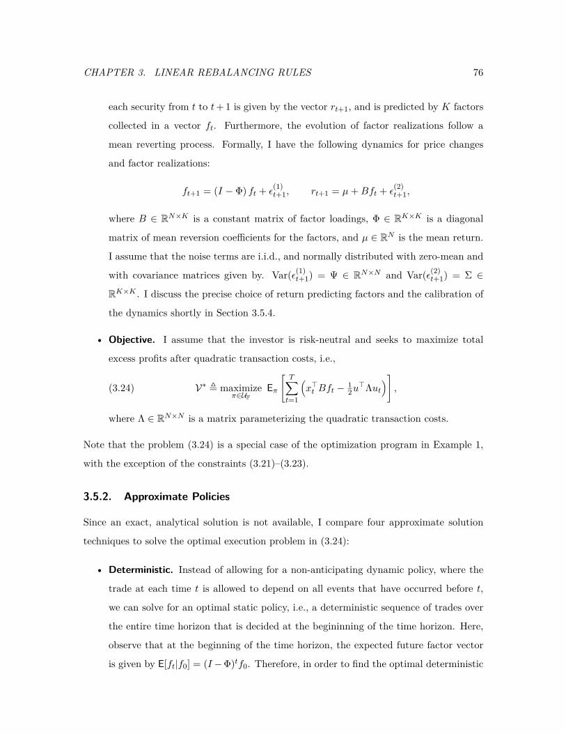
CHAPTER 3. LINEAR REBALANCING RULES 76
each security from t to t+ 1 is given by the vector rt+1, and is predicted by K factors
collected in a vector ft. Furthermore, the evolution of factor realizations follow a
mean reverting process. Formally, I have the following dynamics for price changes
and factor realizations:
ft+1 = (I − Φ) ft + ε(1)t+1, rt+1 = µ+Bft + ε
(2)t+1,
where B ∈ RN×K is a constant matrix of factor loadings, Φ ∈ RK×K is a diagonal
matrix of mean reversion coefficients for the factors, and µ ∈ RN is the mean return.
I assume that the noise terms are i.i.d., and normally distributed with zero-mean and
with covariance matrices given by. Var(ε(1)t+1) = Ψ ∈ RN×N and Var(ε(2)
t+1) = Σ ∈
RK×K . I discuss the precise choice of return predicting factors and the calibration of
the dynamics shortly in Section 3.5.4.
• Objective. I assume that the investor is risk-neutral and seeks to maximize total
excess profits after quadratic transaction costs, i.e.,
(3.24) V∗ , maximizeπ∈UF
Eπ[T∑t=1
(x>t Bft − 1
2u>Λut
)],
where Λ ∈ RN×N is a matrix parameterizing the quadratic transaction costs.
Note that the problem (3.24) is a special case of the optimization program in Example 1,
with the exception of the constraints (3.21)–(3.23).
3.5.2. Approximate Policies
Since an exact, analytical solution is not available, I compare four approximate solution
techniques to solve the optimal execution problem in (3.24):
• Deterministic. Instead of allowing for a non-anticipating dynamic policy, where the
trade at each time t is allowed to depend on all events that have occurred before t,
we can solve for an optimal static policy, i.e., a deterministic sequence of trades over
the entire time horizon that is decided at the begininning of the time horizon. Here,
observe that at the beginning of the time horizon, the expected future factor vector
is given by E[ft|f0] = (I−Φ)tf0. Therefore, in order to find the optimal deterministic
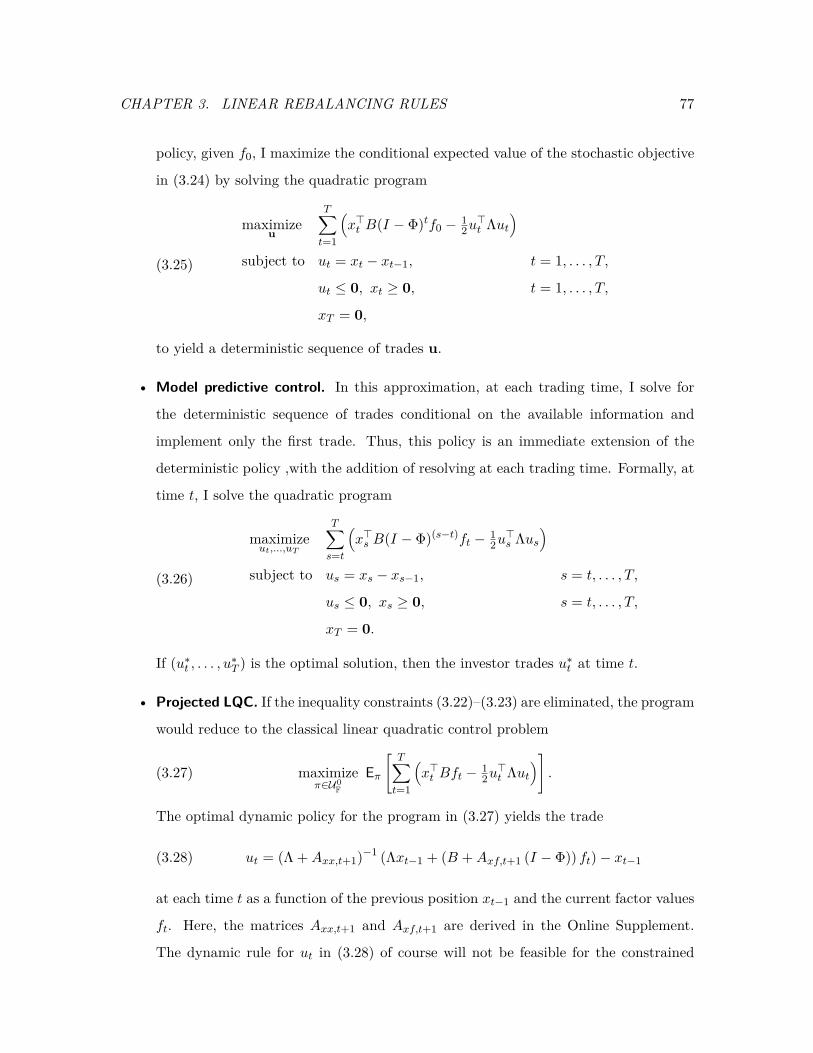
CHAPTER 3. LINEAR REBALANCING RULES 77
policy, given f0, I maximize the conditional expected value of the stochastic objective
in (3.24) by solving the quadratic program
(3.25)
maximizeu
T∑t=1
(x>t B(I − Φ)tf0 − 1
2u>t Λut
)subject to ut = xt − xt−1, t = 1, . . . , T,
ut ≤ 0, xt ≥ 0, t = 1, . . . , T,
xT = 0,
to yield a deterministic sequence of trades u.
• Model predictive control. In this approximation, at each trading time, I solve for
the deterministic sequence of trades conditional on the available information and
implement only the first trade. Thus, this policy is an immediate extension of the
deterministic policy ,with the addition of resolving at each trading time. Formally, at
time t, I solve the quadratic program
(3.26)
maximizeut,...,uT
T∑s=t
(x>s B(I − Φ)(s−t)ft − 1
2u>s Λus
)subject to us = xs − xs−1, s = t, . . . , T,
us ≤ 0, xs ≥ 0, s = t, . . . , T,
xT = 0.
If (u∗t , . . . , u∗T ) is the optimal solution, then the investor trades u∗t at time t.
• Projected LQC. If the inequality constraints (3.22)–(3.23) are eliminated, the program
would reduce to the classical linear quadratic control problem
(3.27) maximizeπ∈U0
F
Eπ[T∑t=1
(x>t Bft − 1
2u>t Λut
)].
The optimal dynamic policy for the program in (3.27) yields the trade
(3.28) ut = (Λ +Axx,t+1)−1 (Λxt−1 + (B +Axf,t+1 (I − Φ)) ft)− xt−1
at each time t as a function of the previous position xt−1 and the current factor values
ft. Here, the matrices Axx,t+1 and Axf,t+1 are derived in the Online Supplement.
The dynamic rule for ut in (3.28) of course will not be feasible for the constrained
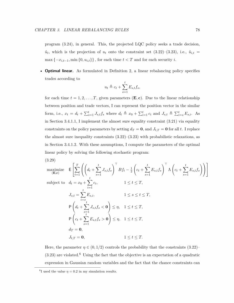
CHAPTER 3. LINEAR REBALANCING RULES 78
program (3.24), in general. This, the projected LQC policy seeks a trade decision,
ut, which is the projection of ut onto the constraint set (3.22)–(3.23), i.e., ui,t =
max −xi,t−1,min 0, ui,t , for each time t < T and for each security i.
• Optimal linear. As formulated in Definition 2, a linear rebalancing policy specifies
trades according to
ut , ct +t∑
s=1Es,tfs,
for each time t = 1, 2, . . . , T , given parameters (E, c). Due to the linear relationship
between position and trade vectors, I can represent the position vector in the similar
form, i.e., xt = dt +∑ts=1 Js,tfs where dt , x0 +
∑ti=1 ci and Js,t ,
∑ti=sEs,i. As
in Section 3.4.1.1, I implement the almost sure equality constraint (3.21) via equality
constraints on the policy parameters by setting dT = 0, and Jt,T = 0 for all t. I replace
the almost sure inequality constraints (3.22)–(3.23) with probabilistic relaxations, as
in Section 3.4.1.2. With these assumptions, I compute the parameters of the optimal
linear policy by solving the following stochastic program:
(3.29)
maximize(E,c)
E
T∑t=1
(dt +t∑
s=1Js,tfs
)>Bft − 1
2
(ct +
t∑s=1
Es,tfs
)>Λ(ct +
t∑s=1
Es,tfs
)subject to dt = x0 +
t∑i=1
ci, 1 ≤ t ≤ T,
Js,t =t∑i=s
Es,i, 1 ≤ s ≤ t ≤ T,
P(dt +
t∑s=1
Js,tfs < 0)≤ η, 1 ≤ t ≤ T,
P(ct +
t∑s=1
Es,tfs > 0)≤ η, 1 ≤ t ≤ T,
dT = 0,
Jt,T = 0, 1 ≤ t ≤ T.
Here, the parameter η ∈ (0, 1/2) controls the probability that the constraints (3.22)–
(3.23) are violated.6 Using the fact that the objective is an expectation of a quadratic
expression in Gaussian random variables and the fact that the chance constraints can6I used the value η = 0.2 in my simulation results.
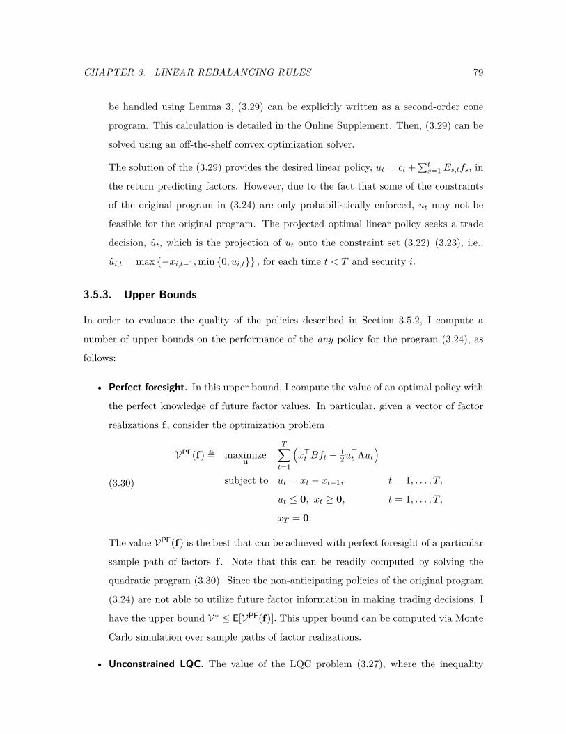
CHAPTER 3. LINEAR REBALANCING RULES 79
be handled using Lemma 3, (3.29) can be explicitly written as a second-order cone
program. This calculation is detailed in the Online Supplement. Then, (3.29) can be
solved using an off-the-shelf convex optimization solver.
The solution of the (3.29) provides the desired linear policy, ut = ct +∑ts=1Es,tfs, in
the return predicting factors. However, due to the fact that some of the constraints
of the original program in (3.24) are only probabilistically enforced, ut may not be
feasible for the original program. The projected optimal linear policy seeks a trade
decision, ut, which is the projection of ut onto the constraint set (3.22)–(3.23), i.e.,
ui,t = max −xi,t−1,min 0, ui,t , for each time t < T and security i.
3.5.3. Upper Bounds
In order to evaluate the quality of the policies described in Section 3.5.2, I compute a
number of upper bounds on the performance of the any policy for the program (3.24), as
follows:
• Perfect foresight. In this upper bound, I compute the value of an optimal policy with
the perfect knowledge of future factor values. In particular, given a vector of factor
realizations f , consider the optimization problem
(3.30)
VPF(f) , maximizeu
T∑t=1
(x>t Bft − 1
2u>t Λut
)subject to ut = xt − xt−1, t = 1, . . . , T,
ut ≤ 0, xt ≥ 0, t = 1, . . . , T,
xT = 0.
The value VPF(f) is the best that can be achieved with perfect foresight of a particular
sample path of factors f . Note that this can be readily computed by solving the
quadratic program (3.30). Since the non-anticipating policies of the original program
(3.24) are not able to utilize future factor information in making trading decisions, I
have the upper bound V∗ ≤ E[VPF(f)]. This upper bound can be computed via Monte
Carlo simulation over sample paths of factor realizations.
• Unconstrained LQC. The value of the LQC problem (3.27), where the inequality
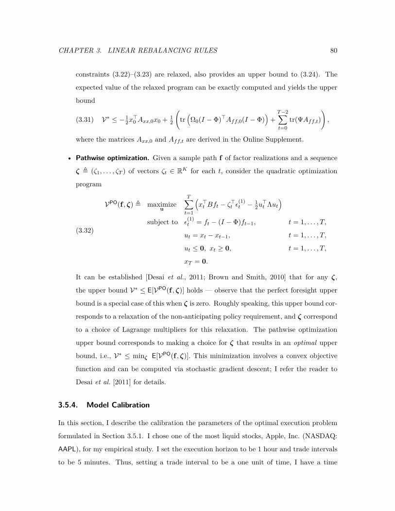
CHAPTER 3. LINEAR REBALANCING RULES 80
constraints (3.22)–(3.23) are relaxed, also provides an upper bound to (3.24). The
expected value of the relaxed program can be exactly computed and yields the upper
bound
(3.31) V∗ ≤ −12x>0 Axx,0x0 + 1
2
(tr(Ω0(I − Φ)>Aff,0(I − Φ)
)+T−2∑t=0
tr(ΨAff,t)),
where the matrices Axx,0 and Aff,t are derived in the Online Supplement.
• Pathwise optimization. Given a sample path f of factor realizations and a sequence
ζ , (ζ1, . . . , ζT ) of vectors ζt ∈ RK for each t, consider the quadratic optimization
program
(3.32)
VPO(f , ζ) , maximizeu
T∑t=1
(x>t Bft − ζ>t ε
(1)t − 1
2u>t Λut
)subject to ε
(1)t = ft − (I − Φ)ft−1, t = 1, . . . , T,
ut = xt − xt−1, t = 1, . . . , T,
ut ≤ 0, xt ≥ 0, t = 1, . . . , T,
xT = 0.
It can be established [Desai et al., 2011; Brown and Smith, 2010] that for any ζ,
the upper bound V∗ ≤ E[VPO(f , ζ)] holds — observe that the perfect foresight upper
bound is a special case of this when ζ is zero. Roughly speaking, this upper bound cor-
responds to a relaxation of the non-anticipating policy requirement, and ζ correspond
to a choice of Lagrange multipliers for this relaxation. The pathwise optimization
upper bound corresponds to making a choice for ζ that results in an optimal upper
bound, i.e., V∗ ≤ minζ E[VPO(f , ζ)]. This minimization involves a convex objective
function and can be computed via stochastic gradient descent; I refer the reader to
Desai et al. [2011] for details.
3.5.4. Model Calibration
In this section, I describe the calibration the parameters of the optimal execution problem
formulated in Section 3.5.1. I chose one of the most liquid stocks, Apple, Inc. (NASDAQ:
AAPL), for my empirical study. I set the execution horizon to be 1 hour and trade intervals
to be 5 minutes. Thus, setting a trade interval to be a one unit of time, I have a time
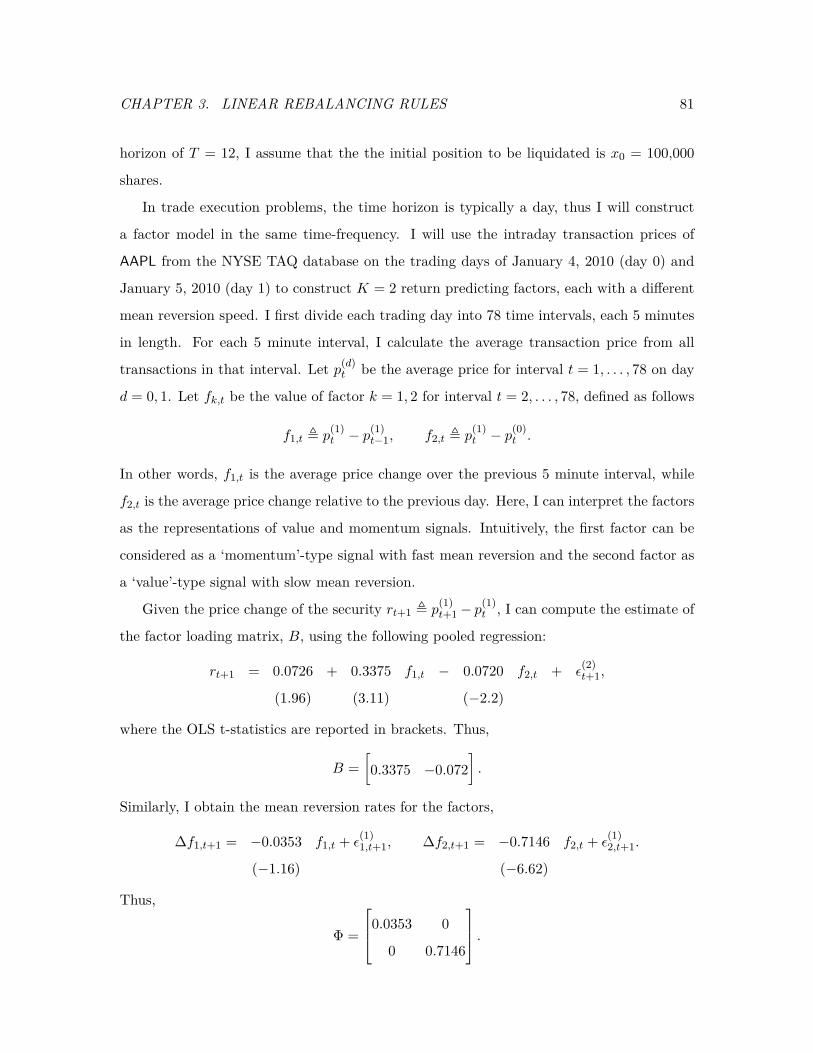
CHAPTER 3. LINEAR REBALANCING RULES 81
horizon of T = 12, I assume that the the initial position to be liquidated is x0 = 100,000
shares.
In trade execution problems, the time horizon is typically a day, thus I will construct
a factor model in the same time-frequency. I will use the intraday transaction prices of
AAPL from the NYSE TAQ database on the trading days of January 4, 2010 (day 0) and
January 5, 2010 (day 1) to construct K = 2 return predicting factors, each with a different
mean reversion speed. I first divide each trading day into 78 time intervals, each 5 minutes
in length. For each 5 minute interval, I calculate the average transaction price from all
transactions in that interval. Let p(d)t be the average price for interval t = 1, . . . , 78 on day
d = 0, 1. Let fk,t be the value of factor k = 1, 2 for interval t = 2, . . . , 78, defined as follows
f1,t , p(1)t − p
(1)t−1, f2,t , p
(1)t − p
(0)t .
In other words, f1,t is the average price change over the previous 5 minute interval, while
f2,t is the average price change relative to the previous day. Here, I can interpret the factors
as the representations of value and momentum signals. Intuitively, the first factor can be
considered as a ‘momentum’-type signal with fast mean reversion and the second factor as
a ‘value’-type signal with slow mean reversion.
Given the price change of the security rt+1 , p(1)t+1− p
(1)t , I can compute the estimate of
the factor loading matrix, B, using the following pooled regression:
rt+1 = 0.0726 + 0.3375 f1,t − 0.0720 f2,t + ε(2)t+1,
(1.96) (3.11) (−2.2)
where the OLS t-statistics are reported in brackets. Thus,
B =[0.3375 −0.072
].
Similarly, I obtain the mean reversion rates for the factors,
∆f1,t+1 = −0.0353 f1,t + ε(1)1,t+1, ∆f2,t+1 = −0.7146 f2,t + ε
(1)2,t+1.
(−1.16) (−6.62)
Thus,
Φ =
0.0353 0
0 0.7146
.
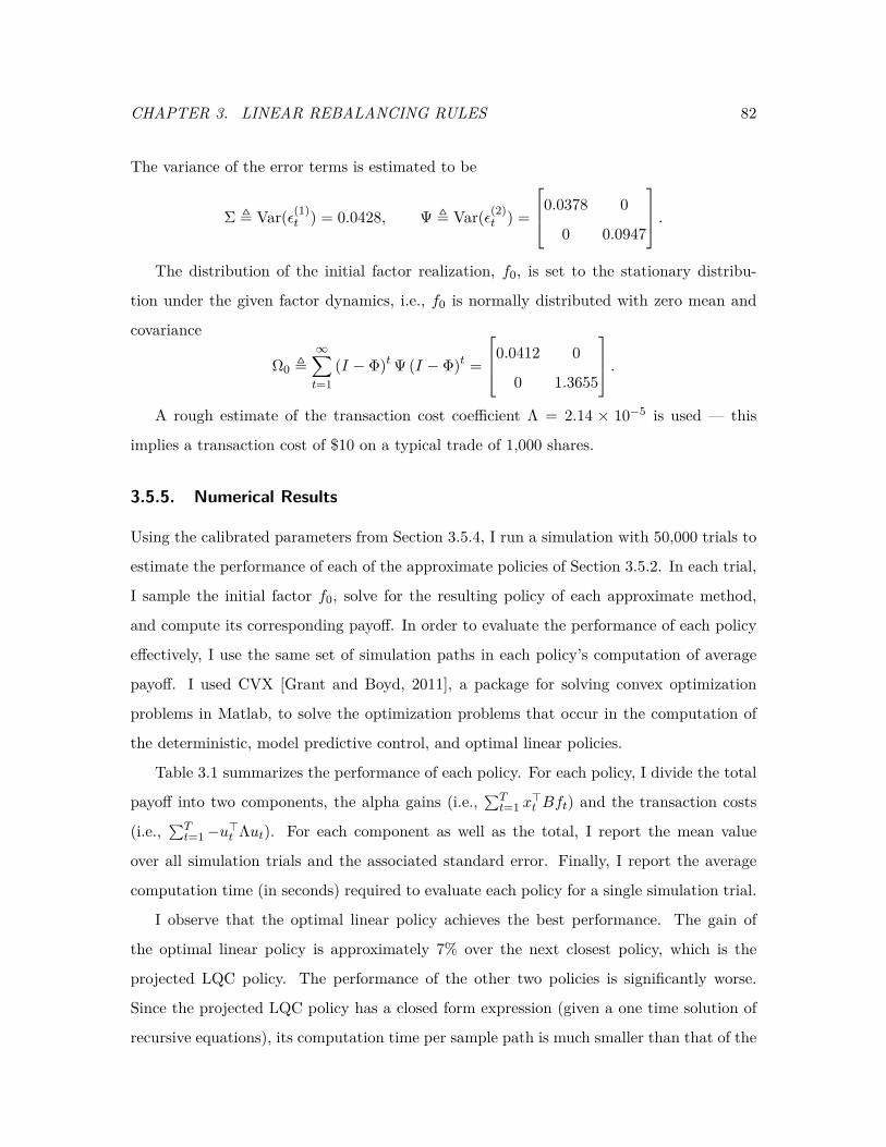
CHAPTER 3. LINEAR REBALANCING RULES 82
The variance of the error terms is estimated to be
Σ , Var(ε(1)t ) = 0.0428, Ψ , Var(ε(2)
t ) =
0.0378 0
0 0.0947
.The distribution of the initial factor realization, f0, is set to the stationary distribu-
tion under the given factor dynamics, i.e., f0 is normally distributed with zero mean and
covariance
Ω0 ,∞∑t=1
(I − Φ)t Ψ (I − Φ)t =
0.0412 0
0 1.3655
.A rough estimate of the transaction cost coefficient Λ = 2.14 × 10⁻⁵ is used — this
implies a transaction cost of $10 on a typical trade of 1,000 shares.
3.5.5. Numerical Results
Using the calibrated parameters from Section 3.5.4, I run a simulation with 50,000 trials to
estimate the performance of each of the approximate policies of Section 3.5.2. In each trial,
I sample the initial factor f0, solve for the resulting policy of each approximate method,
and compute its corresponding payoff. In order to evaluate the performance of each policy
effectively, I use the same set of simulation paths in each policy’s computation of average
payoff. I used CVX [Grant and Boyd, 2011], a package for solving convex optimization
problems in Matlab, to solve the optimization problems that occur in the computation of
the deterministic, model predictive control, and optimal linear policies.
Table 3.1 summarizes the performance of each policy. For each policy, I divide the total
payoff into two components, the alpha gains (i.e.,∑Tt=1 x
>t Bft) and the transaction costs
(i.e.,∑Tt=1−u>t Λut). For each component as well as the total, I report the mean value
over all simulation trials and the associated standard error. Finally, I report the average
computation time (in seconds) required to evaluate each policy for a single simulation trial.
I observe that the optimal linear policy achieves the best performance. The gain of
the optimal linear policy is approximately 7% over the next closest policy, which is the
projected LQC policy. The performance of the other two policies is significantly worse.
Since the projected LQC policy has a closed form expression (given a one time solution of
recursive equations), its computation time per sample path is much smaller than that of the
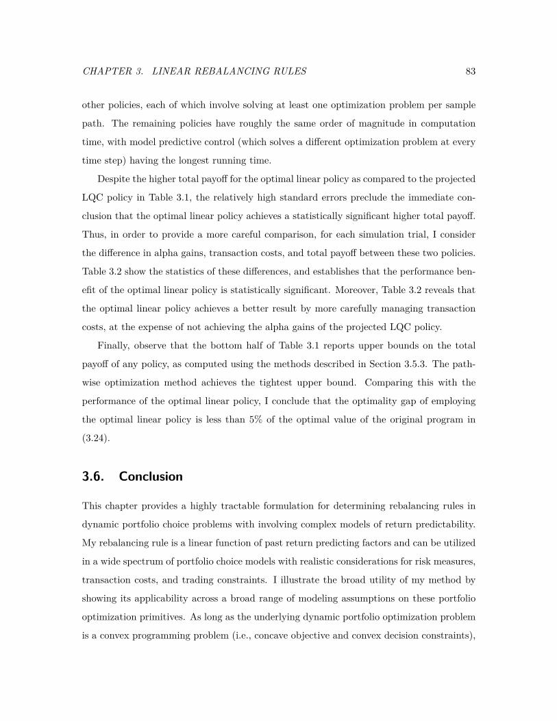
CHAPTER 3. LINEAR REBALANCING RULES 83
other policies, each of which involve solving at least one optimization problem per sample
path. The remaining policies have roughly the same order of magnitude in computation
time, with model predictive control (which solves a different optimization problem at every
time step) having the longest running time.
Despite the higher total payoff for the optimal linear policy as compared to the projected
LQC policy in Table 3.1, the relatively high standard errors preclude the immediate con-
clusion that the optimal linear policy achieves a statistically significant higher total payoff.
Thus, in order to provide a more careful comparison, for each simulation trial, I consider
the difference in alpha gains, transaction costs, and total payoff between these two policies.
Table 3.2 show the statistics of these differences, and establishes that the performance ben-
efit of the optimal linear policy is statistically significant. Moreover, Table 3.2 reveals that
the optimal linear policy achieves a better result by more carefully managing transaction
costs, at the expense of not achieving the alpha gains of the projected LQC policy.
Finally, observe that the bottom half of Table 3.1 reports upper bounds on the total
payoff of any policy, as computed using the methods described in Section 3.5.3. The path-
wise optimization method achieves the tightest upper bound. Comparing this with the
performance of the optimal linear policy, I conclude that the optimality gap of employing
the optimal linear policy is less than 5% of the optimal value of the original program in
(3.24).
3.6. Conclusion
This chapter provides a highly tractable formulation for determining rebalancing rules in
dynamic portfolio choice problems with involving complex models of return predictability.
My rebalancing rule is a linear function of past return predicting factors and can be utilized
in a wide spectrum of portfolio choice models with realistic considerations for risk measures,
transaction costs, and trading constraints. I illustrate the broad utility of my method by
showing its applicability across a broad range of modeling assumptions on these portfolio
optimization primitives. As long as the underlying dynamic portfolio optimization problem
is a convex programming problem (i.e., concave objective and convex decision constraints),
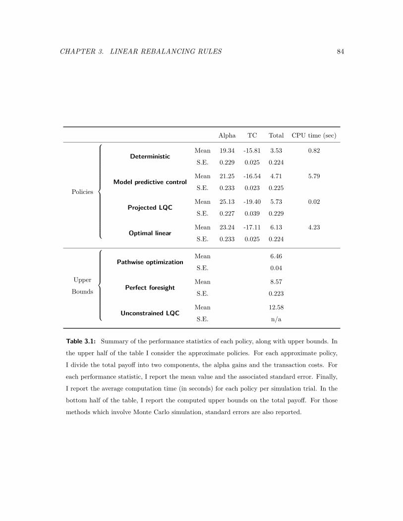
CHAPTER 3. LINEAR REBALANCING RULES 84
Alpha TC Total CPU time (sec)
Policies
DeterministicMean 19.34 -15.81 3.53 0.82
S.E. 0.229 0.025 0.224
Model predictive controlMean 21.25 -16.54 4.71 5.79
S.E. 0.233 0.023 0.225
Projected LQCMean 25.13 -19.40 5.73 0.02
S.E. 0.227 0.039 0.229
Optimal linearMean 23.24 -17.11 6.13 4.23
S.E. 0.233 0.025 0.224
Upper
Bounds
Pathwise optimizationMean 6.46
S.E. 0.04
Perfect foresightMean 8.57
S.E. 0.223
Unconstrained LQCMean 12.58
S.E. n/a
Table 3.1: Summary of the performance statistics of each policy, along with upper bounds. In
the upper half of the table I consider the approximate policies. For each approximate policy,
I divide the total payoff into two components, the alpha gains and the transaction costs. For
each performance statistic, I report the mean value and the associated standard error. Finally,
I report the average computation time (in seconds) for each policy per simulation trial. In the
bottom half of the table, I report the computed upper bounds on the total payoff. For those
methods which involve Monte Carlo simulation, standard errors are also reported.
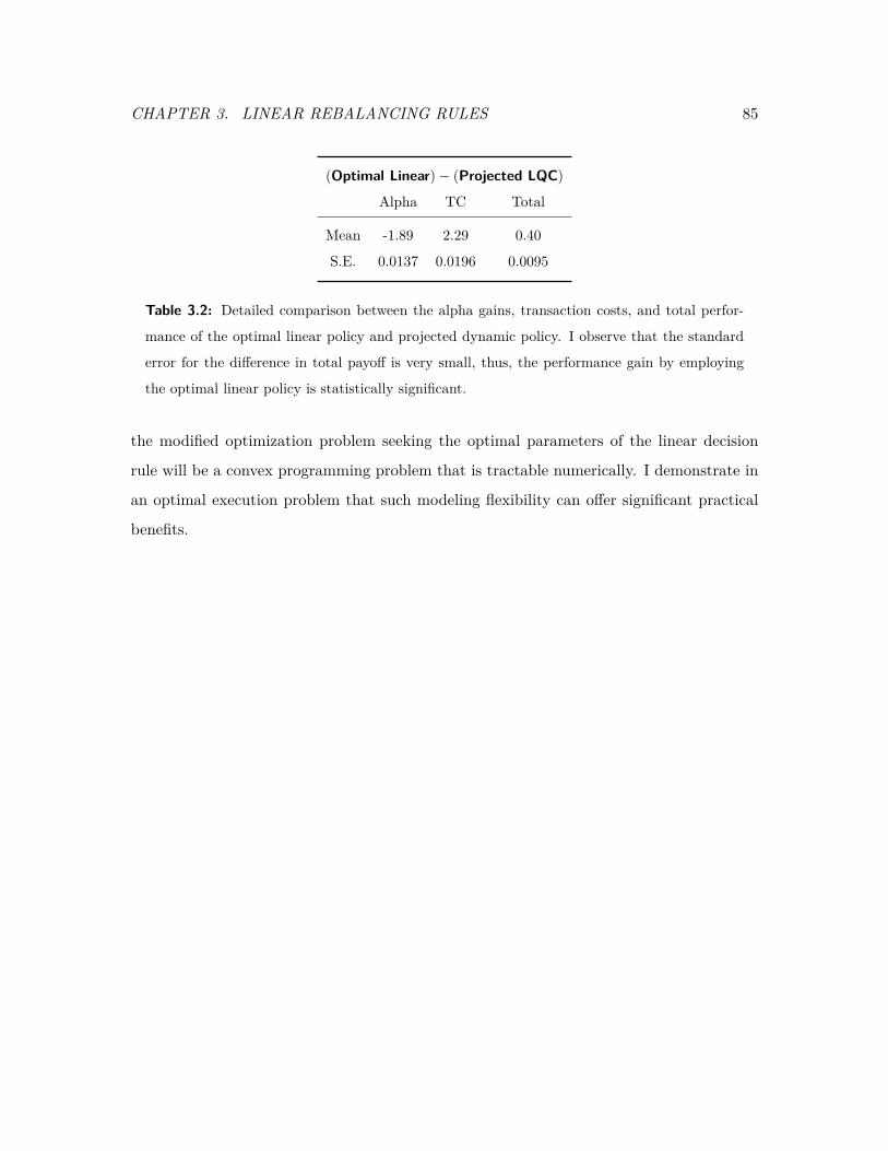
CHAPTER 3. LINEAR REBALANCING RULES 85
(Optimal Linear)− (Projected LQC)
Alpha TC Total
Mean -1.89 2.29 0.40
S.E. 0.0137 0.0196 0.0095
Table 3.2: Detailed comparison between the alpha gains, transaction costs, and total perfor-
mance of the optimal linear policy and projected dynamic policy. I observe that the standard
error for the difference in total payoff is very small, thus, the performance gain by employing
the optimal linear policy is statistically significant.
the modified optimization problem seeking the optimal parameters of the linear decision
rule will be a convex programming problem that is tractable numerically. I demonstrate in
an optimal execution problem that such modeling flexibility can offer significant practical
benefits.
CHAPTER 4. COMMON FACTOR SHOCKS 86
Chapter 4
Common Factor Shocks in Strategic
Asset Allocation
4.1. Introduction
Strategic asset allocation has been a central objective for institutional investors in active
asset management due to changes in the estimates of expected future returns. With the
new estimates for the future returns, the asset manager needs to update the holdings of
the portfolio while aligning with the risk objectives of the fund and keeping trading costs
to a minimum. On top of these tradeoffs, expected future returns are often correlated
with various market conditions such as volatility and liquidity. Characterizing an optimal
rebalancing rule under these complex dynamics, interactions and restrictions is a daunting
task if not impossible.
Many dynamic portfolio choice models need to impose restrictive assumptions, yet often
unrealistic, about return generating model in order to achieve a tractable solution. A recent
simplifying assumption has been using number of shares in the portfolio decision vector in
order to linearize the state dynamics. Using number of shares versus dollar holdings also
required to use price changes in dollars instead of percentage terms. However, it is well-
known that price changes are not stationary, cannot be estimated effectively using linear
regression techniques. In this essay, I keep the nonlinear structure in the wealth evolution
but instead of trying to solve the problem to optimality, I use linear policies in order to
CHAPTER 4. COMMON FACTOR SHOCKS 87
obtain a near-optimal policy. I obtain a closed-form solution for our policy parameters
which allows us to expand the universe of parameters quite easily.
I have tremendous freedom in modeling the dynamics of the return predicting factors. In
a realistic framework, I allow for factor dependent covariance structure in returns driven by
common factor shocks i.e., stochastic volatility. Furthermore, I can also have time-varying
liquidity costs which are correlated with the expected returns of the factors. Our model
involves the standard wealth equation in dollars and nonlinear dynamics for the position
holdings due to the shocks to the existing wealth with current returns.
I provide a well-calibrated simulation study to analyze the performance metrics of our
approach. Our simulation study shows that best linear policy provides significant benefits
compared to other frequently used policies in the literature, especially when the transaction
costs are high and returns evolve according to factor dependent covariance structure. Unlike
other parametric approaches studied so far, our approach provides a closed form solution
and the driver of the policy dynamics can be analyzed in full detail.
4.1.1. Related literature
I addressed a similar review in the previous chapter but I will re-emphasize some of the
references again in this chapter’s context.
The vast literature on dynamic portfolio choice starts with the seminal paper by Merton
[1971] which studies the optimal dynamic allocation of one risky asset and one bond in the
portfolio in a continuous-time setting. Following this seminal paper, there has been a
significant literature aiming to incorporate the impact of various frictions on the optimal
portfolio choice. For a survey on this literature, see Cvitanic [2001]. Constantinides [1986]
studies the impact of proportional transaction costs on the optimal investment decision
and observes path dependence in the optimal policy. Similarly, Davis and Norman [1990],
and Dumas and Luciano [1991a] study the impact of transaction costs on the the optimal
investment and consumption decision by formally characterizing the trade and no-trade
regions. One drawback of all these papers is that the optimal solution is only computed in
the case of a single stock and bond. Liu [2004] extends this result to multiple assets but
assumes that asset returns are not correlated.
CHAPTER 4. COMMON FACTOR SHOCKS 88
There is a growing literature on portfolio selection that incorporates return predictability
with transaction costs. Balduzzi and Lynch [1999] and Lynch and Balduzzi [2000] illustrate
the impact of return predictability and transaction costs on the utility costs and the op-
timal rebalancing rule by discretizing the state space of the dynamic program. Recently,
Brown and Smith [2010] provides heuristic trading strategies and dual bounds for a general
dynamic portfolio optimization problem with transaction costs and return predictability.
Brandt et al. [2009a] parameterizes the rebalancing rule as a function of security charac-
teristics and estimates the parameters of the rule from empirical data without modeling
the distribution of the returns and the return predicting factors. Our approach is also a
linear parametrization of return predicting factors, but at the micro-level, I seek to obtain
a policy that is coherent with the update of the position holdings in a nonlinear fashion.
Thus, our linear policy uses the convolution of the factors with their corresponding returns
in order to correctly satisfy the wealth equation at all times. On a separate note, I solve
for the optimal policy in closed-form using a deterministic linear quadratic control and can
achieve greater flexibility in parameterizing the trading rule.
Garleanu and Pedersen [2012] achieve a closed-form solution for a model with linear
dynamics in return predictors and quadratic function for transaction costs and quadratic
penalty term for risk. However, the model for the security returns is given in price changes
which suffers highly from non-stationarity. This use of price changes is highly nonstandard
and cannot be accommodated with the existing models for return predictability that almost
always uses percentage returns.
4.2. Model
4.2.1. Security and factor dynamics
I consider a dynamic portfolio optimization problem with K factors and N securities. Let
Si,t be the discrete time dynamics for the price of the security that pays a dividend Di,t at
time t. I assume that the gross return to our security defined by Ri,t+1 = Si,t+1+Di,t+1Si,t
have
the following form:
Ri,t+1 = g(t, B>i,t(Ft+1 + λ) + εi,t+1) i = 1, . . . , N

CHAPTER 4. COMMON FACTOR SHOCKS 89
for some family of functions g(t, ·) : R→ R, increasing in their second argument, and where
I further introduce the following notation:
• Bi,t is the (K, 1) vector of exposures to the factors.
• Ft+1 is the (K, 1) vector of random (as of time t) factor realizations, with mean 0 and
conditional covariance matrix Ωt,t+1.
• εi,t+1 is the idiosyncratic risk of stock i.
I assume that ε·,t+1 are mean zero, have a time-invariant covariance matrix Σε, and
are uncorrelated with the contemporaneous factor realizations.
• λt is the (K, 1) vector of conditional expected factor returns
I assume that Bi,t and λt are observable and follow some known dynamics, which for
now I leave unspecified (when I solve a special example below, I assume that λt is constant
and that the Bi,t follow a Gaussian AR(1) process, but our approach could apply to more
complex dynamics). As I show below, our approach can be extended to account for time
varying factor expected returns (i.e., λt could be stochastic), and non-normal factor or
idiosyncratic risk distributions (e.g., GARCH features can easily be added).
Note that this setting captures two standard return generating processes:
1. The “discrete exponential affine” model for security returns in which log-returns
are affine in factor realizations:1
logRi,t+1 = αi +B>i,t(Ft+1 + λ) + εi,t+1 −12(σ2i +B>i,tΩBi,t
)2. The “linear affine factor model” where returns (and therefore also excess returns)
are affine in factor exposures:
ri,t+1 = αi +B>i,t(Ft+1 + λ) + εi,t+1
As I show below, our portfolio optimization approach is equally tractable for both these
return generating processes.1The continuous time version of this model is due to Vasicek [1977], Cox et al. [1985], and generalized in
Duffie and Kan [1996]. The discrete time version is due to Gourieroux et al. [1993] and Le et al. [2010].

CHAPTER 4. COMMON FACTOR SHOCKS 90
4.2.2. Cash and stock position dynamics
I will assume discrete time dynamics for our cash (w(t)) position and dollar holdings (xi(t))
in stocks. I assume that
xi,t+1 = xi,tRi,t+1 + ui,t+1 i = 1, . . . , N
wt+1 = wtR0,t+1 −N∑i=1
ui,t+1 −12
N∑i=1
N∑j=1
ui,t+1Λt+1(i, j)uj,t+1
where Ri,t+1 = Si,t+1+Di,t+1Si,t
is the total gross return (capital gains plus dividends) on the
security i. I am here effectively assuming that each position in security i = 1, . . . , n is
financed by a short position in a (e.g., risk-free) benchmark security 0, which I assume can
be traded with no transaction costs. I denote by xi,t the dollar investment in asset i, by
wt the total cash balances (invested in the risk-free security S0), and ui,t+1 is the dollar
amount of security i I will trade at price Si,t+1. In vector notation,
xt+1 = xt Rt+1 + ut+1(4.1)
wt+1 = wtR0,t+1 − 1>ut+1 −12u>t+1Λt+1ut+1(4.2)
where the operator denotes element by element multiplication if the matrices are of same
size or if the operation involves a scalar and a matrix, then that scalar multiplies every
entry of the matrix.
The matrix Λt captures (possibly time-varying) quadratic transaction/price-impact costs,
so that 12u>t Λtut is the dollar cost paid when realizing a trade at time t of size ut. For sim-
plicity I assume this matrix is symmetric.2 Garleanu and Pedersen [2012] present some
micro-economic foundations for such quadratic costs. As they show, the quadratic form is
analytically very convenient.
4.2.3. Objective function
I assume that the investor’s objective function is to maximize a linear quadratic function
of his terminal cash and stock positions F (wT , xT ) = wT + a>xT − 12x>T b xT , net of a risk-
penalty which I take to be proportional to the per-period variance of the portfolio. I assume2The symmetry assumption could easily be relaxed.
CHAPTER 4. COMMON FACTOR SHOCKS 91
a is a (N, 1) vector and b a (N,N) symmetric matrix.3 So I assume the objective function
is simply:
(4.3) maxu1,...,uT
E[F (wT , xT )−
T−1∑t=0
γ
2x>t Σt→t+1xt
]I define Σt→t+1 = Et[(Rt+1 − Et[Rt+1])(Rt+1 − Et[Rt+1])′] to be the conditional one-
period variance-covariance matrix of returns and γ can be interpreted as the coefficient of
risk aversion.
The F (·, ·) function parameters can be chosen to capture different objectives, such as
maximizing the terminal gross value of the position (wT +1>xT ) or the terminal liquidation
(i.e., net of transaction costs) value of the portfolio (wT + 1>xT − 12x>T ΛTxT ), or any
intermediate situation.
Assuming the investor starts with some initial cash balances w0 and an initial position
in individual stocks x0, note that xT and wT can be rewritten as:
xT = x0 R0→T +T∑i=1
ut Rt→T(4.4)
wT = w0R0,0→T −T∑i=1
(u>t 1R0,t→T + 1
2u>t ΛtutR0,t→T
)(4.5)
where I have defined the cumulative return between date t and T on security i as:
(4.6) Ri,t→T =T∏
s=t+1Ri,s
(with the convention that Ri,t→t = 1) and the corresponding N -dimensional vector Rt→T =
[R1,t→T ; . . . ;RN,t→T ].
Now note that
a>xT = (a R0→T )>x0 +T∑i=1
(a Rt→T )>ut(4.7)
x>T bxT = x>0 RbR0x0 +T∑t=1
u>t RbRtut + 2T∑t=1
x0 R0,t→T bRtut(4.8)
where I define the (N,N)-matrix RbRt and bRtwith respective element:
RbRtij = Ri,t→T bijRj,t→T(4.9)
bRtij = bijRj,t→T(4.10)
3The symmetry assumption on b could easily be relaxed.
CHAPTER 4. COMMON FACTOR SHOCKS 92
Substituting I obtain the following:
F (wT , xT ) = F0 +T∑i=1
G>t ut −
12u>t Ptut
(4.11)
F0 = w0R0,0→T + (a R0→T )>x0 −12x>0 RbR0x0(4.12)
Gt = a Rt→T + 1 R0,t→T − x0 R0,t→T bRt(4.13)
Pt = (RbRt + Λt R0,t→T )(4.14)
Substituting into the objective function given in equation 4.3 it can be rewritten as:
(4.15) F0 + maxu1,...,uT
T−1∑t=0
E[G>t+1ut+1 −
12u>t+1Pt+1ut+1 −
γ
2x>t Σt→t+1xt
]
subject to the non-linear dynamics given in equations 4.1 and 4.2.
I next describe our set of linear policies, which make this problem tractable. At this
stage it is convenient to introduce the following notation (inspired from matlab): I write
[A;B] (respectively [AB]) to denote the vertical (respectively horizontal) concatenation of
two matrices.
4.2.4. Linear policies
I consider a class of parametric linear policies that is richer than the one previously consid-
ered in the literature (see, e.g., Brandt et al. [2009b]), but nevertheless has the advantage
of leading to an explicit solution for the portfolio choice problem with transaction costs.
Thus, in contrast to the approach proposed in Brandt et al. [2009b]), I do not need to
perform a numerical optimization, and can handle transaction costs efficiently. Further, in
contrast to Garleanu and Pedersen [2012] I can handle more complex asset return dynamics
and explicitly formulate the problem in terms of dollar returns (as opposed to number of
shares), and yet retain the analytical flexibility of the linear-quadratic framework.
These benefits come at a cost, namely that of restricting our optimization to a specific
set of parametrized trading strategies. It is an empirical question whether the set I work
with is sufficiently large to deliver useful results. I present some empirical tests of our
approach in the next section. First, I describe the strategy set I consider. Then I explain
how the portfolio optimization can be done in closed-form, within that restricted set.
CHAPTER 4. COMMON FACTOR SHOCKS 93
I define our set of linear policies with a set of (K+1)-dimensional vectors of parameters,
πi,s,t and θi,s,t, defined for all i = 1, . . . , N and for all s ≤ t. The (previously defined) time
t trade of asset i (ui,t) of and dollar investment in asset i (xi,t) are given by:
(4.16) ui,t =t∑
u=1π>i,u,tBi,u,t
and
(4.17) xi,t =t∑
u=1θ>i,u,tBi,u,t
are then vector products of πi,s,t and θi,s,t and a (K + 1) vector
(4.18) Bi,u,t = [1;Bi,t]Ri,u→t .
Bi,u,t is seen to be the (K) vector of time t factor exposures, augmented with a “1”, and
all weighted by the cumulative return earned by security i between time u and t. In other
words, these policies allow trades at time t to depend on current factor exposures Bi,t, but
also on all past exposures weighted by their past holding period returns.
Intuitively, the dependence on current exposures, unweighted by lagged returns, is
clearly important. In fact, in a no-transaction cost affine portfolio optimization problem
where the optimal solution is well-known, the optimal solution will involve only current ex-
posures (see, e.g.,?). Note that this is also the choice made by Brandt et al. [2009b] for their
‘parameteric portfolio policies.’ However, while Brandt et al. [2009b] specify the loadings
on exposure of individual stocks to be identical, I allow two stocks with identical exposures
(and with perhaps different levels of idiosyncratic variance) to have different weights and
trades.4
With transaction costs, allowing portfolio weights and trades to depend on past reutrns
interacted with past exposures seems useful. The intuition for this comes from the path-
dependence I observe in known closed-form solutions [see Constantinides, 1986; Davis and
Norman, 1990; Dumas and Luciano, 1991b; Liu and Loewenstein, 2002, and others]
To proceed, I note that the assumed linear position and trading strategies in equa-
tions 4.42 and 4.41 have to satisfy the dynamics given in equations 4.1 and 4.2. It follows4(Note, for the Brandt et al. [2009b] econometric approach it is useful to have fewer parameters. This is
not an issue with our approach as our solution is closed-form.

CHAPTER 4. COMMON FACTOR SHOCKS 94
that the parameter vectors πi,s,t and θi,s,t have to satisfy the following restrictions, for all
i = 1, . . . , N :
πi,s,t = θi,s,t − θi,s,t−1 for s < t(4.19)
πi,t,t = θi,t,t(4.20)
I can rewrite these policies in a concise matrix form. First, define the (N(K+1)t, 1) vectors
πt and θt as
πt = [π1,1,t; . . . ;πn,1,t;π1,2,t; . . . ;πn,2,t; . . . ;π1,t,t; . . . ;πn,t,t](4.21)
θt = [θ1,1,t; . . . ; θn,1,t; θ1,2,t; . . . ; θn,2,t; . . . ; θ1,t,t; . . . ; θn,t,t](4.22)
Further, let’s define the following (N(K + 1), N) matrices (defined for all 1 ≤ s ≤ t ≤ T )
as the diagonal concatenations of the N vectors Bi,s,t ∀i = 1, . . . , N :
Bs,t =
B1,s,t 0 0 . . . 0
0 B2,s,t 0 . . . 0
. . .
0 . . . 0 Bn,s,t
Then I can define the (N(K + 1)t,N) matrix Bt by stacking the t matrices Bs,t ∀s =
1, . . . , t:
Bt = [B1,t;B2,t, . . . ,Bt,t]
It is then straightforward to check that:
ut = B>t πt(4.23)
xt = B>t θt(4.24)
Further, in terms of these definitions the constraints on the parameter vector in 4.19 can
be rewritten concisely as:
(4.25) θt+1 − θ0t = πt+1
where I define θ0t = [θt; 0K+1] to be the vector θt stacked on top of a (K + 1, 1) vector of
zeros 0K+1.
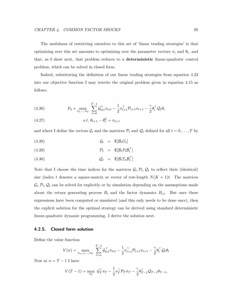
CHAPTER 4. COMMON FACTOR SHOCKS 95
The usefulness of restricting ourselves to this set of ‘linear trading strategies’ is that
optimizing over this set amounts to optimizing over the parameter vectors πt and θt, and
that, as I show next, that problem reduces to a deterministic linear-quadratic control
problem, which can be solved in closed form.
Indeed, substituting the definition of our linear trading strategies from equation 4.23
into our objective function I may rewrite the original problem given in equation 4.15 as
follows.
F0 + maxπ1,...,πT
T−1∑t=0G>t+1πt+1 −
12π>t+1Pt+1πt+1 −
γ
2 θ>t Qtθt(4.26)
s.t. θt+1 − θ0t = πt+1(4.27)
and where I define the vectors Gt and the matrices Pt and Qt defined for all t = 0, . . . , T by
Gt = E[BtGt](4.28)
Pt = E[BtPtB>t ](4.29)
Qt = E[BtΣtB>t ](4.30)
Note that I choose the time indices for the matrices Gt,Pt,Qt to reflect their (identical)
size (index t denotes a square-matrix or vector of row-length N(K + 1)t. The matrices
Gt,Pt,Qt can be solved for explicitly or by simulation depending on the assumptions made
about the return generating process Rt and the factor dynamics Bi,t. But once these
expressions have been computed or simulated (and this only needs to be done once), then
the explicit solution for the optimal strategy can be derived using standard deterministic
linear-quadratic dynamic programming. I derive the solution next.
4.2.5. Closed form solution
Define the value function
V (n) = maxπn+1,...,πT
T−1∑t=nG>t+1πt+1 −
12π>t+1Pt+1πt+1 −
γ
2 θ>t Qtθt
Now at n = T − 1 I have
V (T − 1) = maxπTG>T πT −
12π>T PTπT −
γ
2 θ>T−1QT−1θT−1,

CHAPTER 4. COMMON FACTOR SHOCKS 96
which yields the solution π∗T = P−1T GT and the value function V (T − 1) = 1
2G>T P−1T−1GT −
γ2θ>T−1QT−1θT−1. I therefore guess that the value function is of the form:
(4.31) V (n) = −12θ>nMnθn + L>n θn +Hn
The Hamilton-Jacobi-Bellman equation is
V (t) = maxπt+1
G>t+1πt+1 −
12π>t+1Pt+1πt+1 −
γ
2 θ>t Qtθt + V (t+ 1)
(4.32)
s.t. θt+1 − θ0t = πt+1(4.33)
The first order condition is:
Gt+1 + Lt+1 − (Pt+1 +Mt+1)πt+1 = Mt+1θ0t
which gives the optimal trade (and corresponding) state equation:
πt+1 = [Pt+1 +Mt+1]−1(Gt+1 + Lt+1 −Mt+1θ0t )(4.34)
θt+1 = [Pt+1 +Mt+1]−1(Gt+1 + Lt+1 + Pt+1θ0t )(4.35)
The HJB equation can be rewritten with our guess as
V (t) = π>t+1
(Gt+1 + Lt+1 −
12(Pt+1 +Mt+1)πt+1
)−1
2θ0tMt+1(θ0
t )>−π>t+1Mt+1θ0t−
γ
2 θ>t Qtθt+Ht+1+L>t+1θ
0t
Now, for a [N(K + 1)t,N(K + 1)t] dimensional square matrix Xt I define Xt to be the
upper left-hand corner square submatrix with dimensions [N(K+1)(t−1), N(K+1)(t−1)].
Using this definition and substituting the FOC I get:
V (t) = 12(Gt+1 + Lt+1 −Mt+1θ
0t )>[Pt+1 +Mt+1]−1(Gt+1 + Lt+1 −Mt+1θ
0t )−
12θ>t (M t+1 + γQt)θt
+Ht+1 + L>t+1θ0t
which I can simplify further:
V (t) = 12(Gt+1 + Lt+1)>[Pt+1 +Mt+1]−1(Gt+1 + Lt+1)− 1
2θ>t
(M t+1 + γQt
−Mt+1[Pt+1 +Mt+1]−1Mt+1)θt +Ht+1 + (Lt+1 +Mt+1[Pt+1 +Mt+1]−1(Gt+1 + Lt+1))>θ0
t
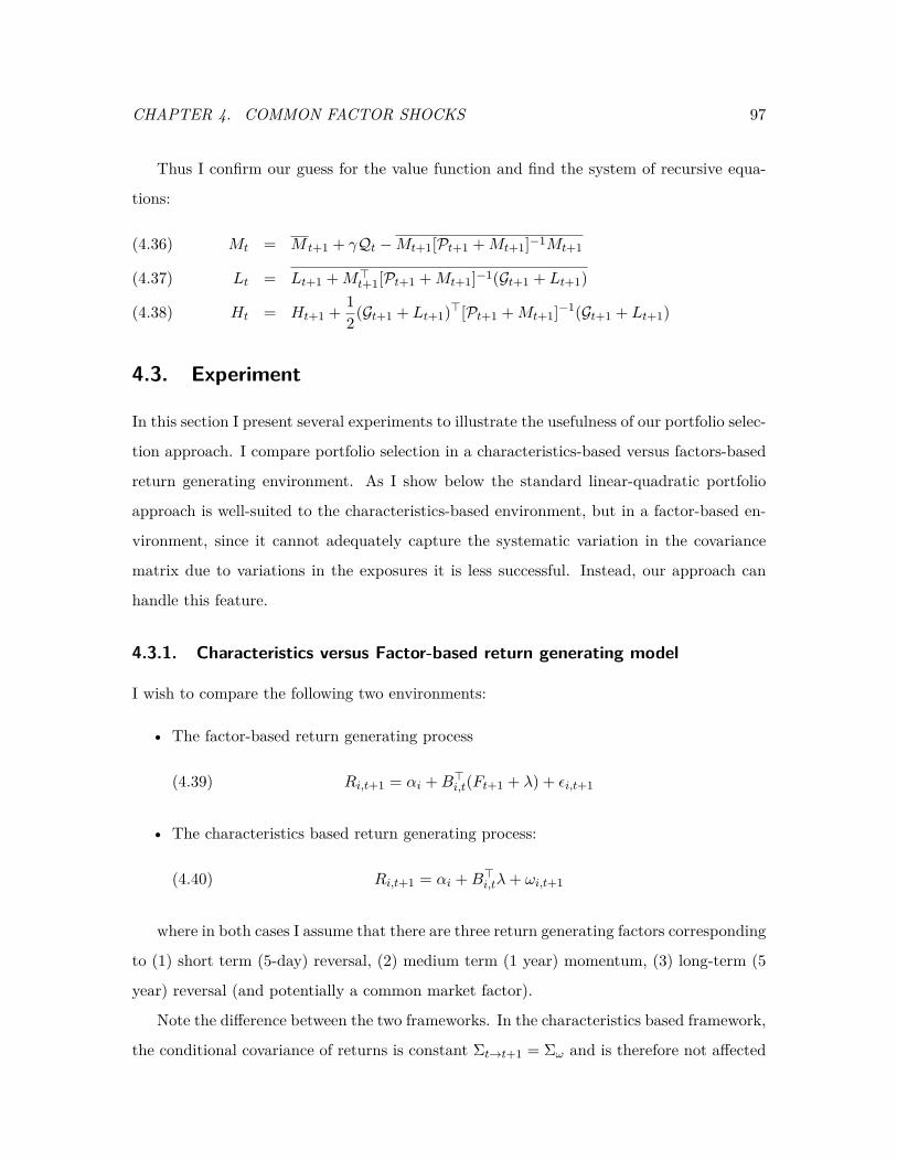
CHAPTER 4. COMMON FACTOR SHOCKS 97
Thus I confirm our guess for the value function and find the system of recursive equa-
tions:
Mt = M t+1 + γQt −Mt+1[Pt+1 +Mt+1]−1Mt+1(4.36)
Lt = Lt+1 +M>t+1[Pt+1 +Mt+1]−1(Gt+1 + Lt+1)(4.37)
Ht = Ht+1 + 12(Gt+1 + Lt+1)>[Pt+1 +Mt+1]−1(Gt+1 + Lt+1)(4.38)
4.3. Experiment
In this section I present several experiments to illustrate the usefulness of our portfolio selec-
tion approach. I compare portfolio selection in a characteristics-based versus factors-based
return generating environment. As I show below the standard linear-quadratic portfolio
approach is well-suited to the characteristics-based environment, but in a factor-based en-
vironment, since it cannot adequately capture the systematic variation in the covariance
matrix due to variations in the exposures it is less successful. Instead, our approach can
handle this feature.
4.3.1. Characteristics versus Factor-based return generating model
I wish to compare the following two environments:
• The factor-based return generating process
(4.39) Ri,t+1 = αi +B>i,t(Ft+1 + λ) + εi,t+1
• The characteristics based return generating process:
(4.40) Ri,t+1 = αi +B>i,tλ+ ωi,t+1
where in both cases I assume that there are three return generating factors corresponding
to (1) short term (5-day) reversal, (2) medium term (1 year) momentum, (3) long-term (5
year) reversal (and potentially a common market factor).
Note the difference between the two frameworks. In the characteristics based framework,
the conditional covariance of returns is constant Σt→t+1 = Σω and is therefore not affected

CHAPTER 4. COMMON FACTOR SHOCKS 98
by the factor exposures. Instead, in the factor-based framework, the conditional covariance
matrix of returns is time varying: Σt→t+1 = BtΩB>t + Σε where Bt = [B>1,t;B>2,t; . . . ;B>n,t]
is the (N,K) matrix of factor exposures.
I assume that the half-life of the 5-day factor is 3 days, that of the one-year factor is
150 days, that of the 5-year factor is 700 days. I define the exposure dynamics using the
simple auto-regressive process:
Bki,t+1 = (1− φk)Bk
i,t + εi,t+1.
The value of φk is tied to its half-life (expressed in number of days) hk by the simple
relation φk = (12)hk .
For the case, where I investigate the ‘Characteristics based’ model I set the constant
covariance matrix Σω so that it matches the unconditional covariance matrix of the factor
based return generating process, i.e., I set
Σω = E[BtΩB>t + Σε]
Note that
BtΩB>t =K∑
l,m=1Ωl,mB
l:,t(Bm
:,t)>
where Bk:,t is the factor values of each asset corresponding to the kth factor at time t.
4.3.2. Calibration of main parameters
The number of assets in our experiment is 15. One can think of these as a collection
of portfolios instead of individual stocks, e.g., stock or commodity indices. Our trading
horizon is 26 weeks with weekly rebalancing. Our objective is to maximize net terminal
wealth minus penalty terms for excessive risk. This requires us to set a = 1 and b = 0 in
our objective function.
I calibrate the factor mean, λ, and covariance matrix, Ω, using Fama-French 10 portfolios
sorted on short-term reversal, momentum, and long term reversal. Using monthly returns,
I compute the performance of the long-short portfolio for the highest and lowest decile in
each factor data. Obtaining 3 long-short portfolios, I set λ to be its mean and Ω to be its
covariance matrix. Table 4.1 illustrates the estimated values for λ and Ω.
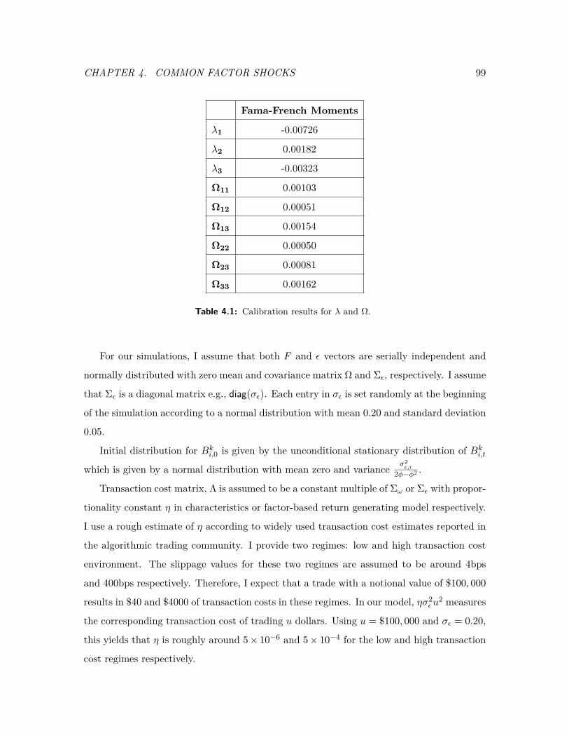
CHAPTER 4. COMMON FACTOR SHOCKS 99
Fama-French Moments
λ1 -0.00726
λ2 0.00182
λ3 -0.00323
Ω11 0.00103
Ω12 0.00051
Ω13 0.00154
Ω22 0.00050
Ω23 0.00081
Ω33 0.00162
Table 4.1: Calibration results for λ and Ω.
For our simulations, I assume that both F and ε vectors are serially independent and
normally distributed with zero mean and covariance matrix Ω and Σε, respectively. I assume
that Σε is a diagonal matrix e.g., diag(σε). Each entry in σε is set randomly at the beginning
of the simulation according to a normal distribution with mean 0.20 and standard deviation
0.05.
Initial distribution for Bki,0 is given by the unconditional stationary distribution of Bk
i,t
which is given by a normal distribution with mean zero and variance σ2ε,i
2φ−φ2 .
Transaction cost matrix, Λ is assumed to be a constant multiple of Σω or Σε with propor-
tionality constant η in characteristics or factor-based return generating model respectively.
I use a rough estimate of η according to widely used transaction cost estimates reported in
the algorithmic trading community. I provide two regimes: low and high transaction cost
environment. The slippage values for these two regimes are assumed to be around 4bps
and 400bps respectively. Therefore, I expect that a trade with a notional value of $100, 000
results in $40 and $4000 of transaction costs in these regimes. In our model, ησ2εu
2 measures
the corresponding transaction cost of trading u dollars. Using u = $100, 000 and σε = 0.20,
this yields that η is roughly around 5× 10⁻⁶ and 5× 10⁻⁴ for the low and high transaction
cost regimes respectively.
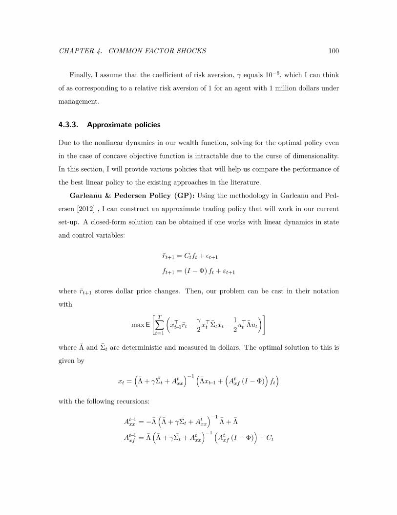
CHAPTER 4. COMMON FACTOR SHOCKS 100
Finally, I assume that the coefficient of risk aversion, γ equals 10−6, which I can think
of as corresponding to a relative risk aversion of 1 for an agent with 1 million dollars under
management.
4.3.3. Approximate policies
Due to the nonlinear dynamics in our wealth function, solving for the optimal policy even
in the case of concave objective function is intractable due to the curse of dimensionality.
In this section, I will provide various policies that will help us compare the performance of
the best linear policy to the existing approaches in the literature.
Garleanu & Pedersen Policy (GP): Using the methodology in Garleanu and Ped-
ersen [2012] , I can construct an approximate trading policy that will work in our current
set-up. A closed-form solution can be obtained if one works with linear dynamics in state
and control variables:
rt+1 = Ctft + εt+1
ft+1 = (I − Φ) ft + εt+1
where rt+1 stores dollar price changes. Then, our problem can be cast in their notation
with
max E[T∑t=1
(x>t−1rt −
γ
2x>t Σtxt −
12u>t Λut
)]
where Λ and Σt are deterministic and measured in dollars. The optimal solution to this is
given by
xt =(Λ + γΣt +Atxx
)−1 (Λxt−1 +
(Atxf (I − Φ)
)ft)
with the following recursions:
At−1xx = −Λ
(Λ + γΣt +Atxx
)−1Λ + Λ
At−1xf = Λ
(Λ + γΣt +Atxx
)−1 (Atxf (I − Φ)
)+ Ct
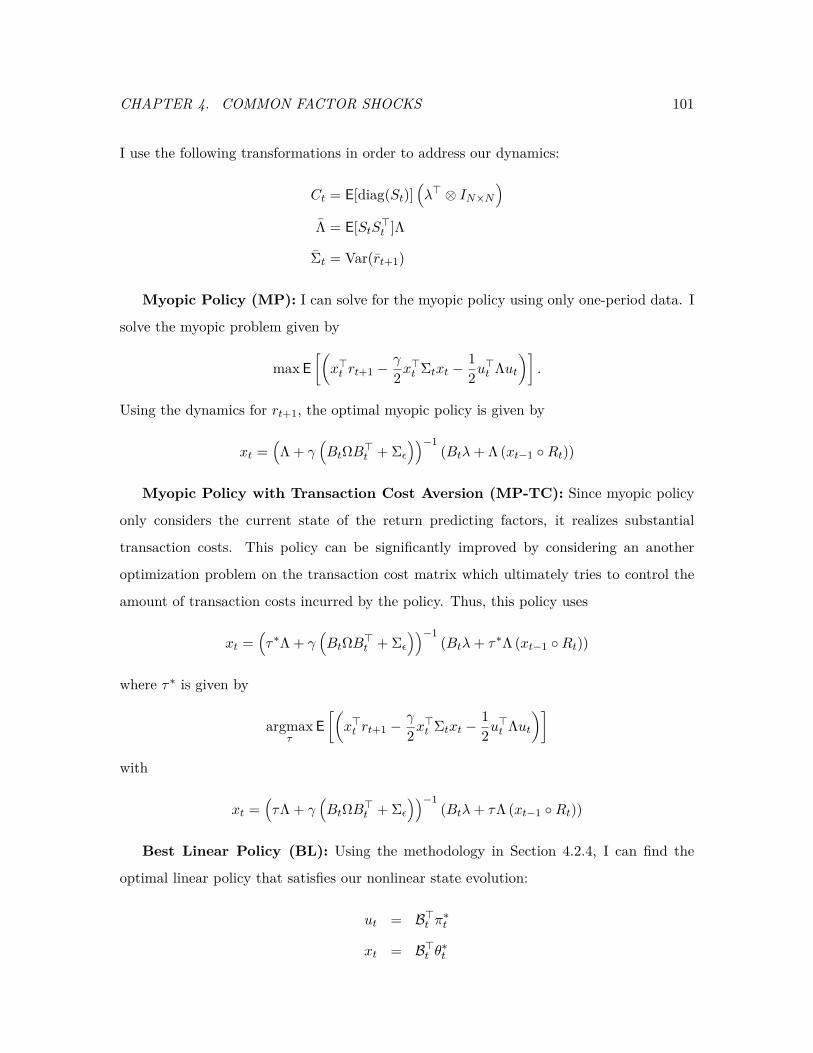
CHAPTER 4. COMMON FACTOR SHOCKS 101
I use the following transformations in order to address our dynamics:
Ct = E[diag(St)](λ> ⊗ IN×N
)Λ = E[StS>t ]Λ
Σt = Var(rt+1)
Myopic Policy (MP): I can solve for the myopic policy using only one-period data. I
solve the myopic problem given by
max E[(x>t rt+1 −
γ
2x>t Σtxt −
12u>t Λut
)].
Using the dynamics for rt+1, the optimal myopic policy is given by
xt =(Λ + γ
(BtΩB>t + Σε
))−1(Btλ+ Λ (xt−1 Rt))
Myopic Policy with Transaction Cost Aversion (MP-TC): Since myopic policy
only considers the current state of the return predicting factors, it realizes substantial
transaction costs. This policy can be significantly improved by considering an another
optimization problem on the transaction cost matrix which ultimately tries to control the
amount of transaction costs incurred by the policy. Thus, this policy uses
xt =(τ∗Λ + γ
(BtΩB>t + Σε
))−1(Btλ+ τ∗Λ (xt−1 Rt))
where τ∗ is given by
argmaxτ
E[(x>t rt+1 −
γ
2x>t Σtxt −
12u>t Λut
)]with
xt =(τΛ + γ
(BtΩB>t + Σε
))−1(Btλ+ τΛ (xt−1 Rt))
Best Linear Policy (BL): Using the methodology in Section 4.2.4, I can find the
optimal linear policy that satisfies our nonlinear state evolution:
ut = B>t π∗t
xt = B>t θ∗t
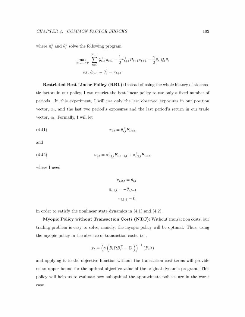
CHAPTER 4. COMMON FACTOR SHOCKS 102
where π∗t and θ∗t solve the following program
maxπ1,...,πT
T−1∑t=0G>t+1πt+1 −
12π>t+1Pt+1πt+1 −
γ
2 θ>t Qtθt
s.t. θt+1 − θ0t = πt+1
Restricted Best Linear Policy (RBL): Instead of using the whole history of stochas-
tic factors in our policy, I can restrict the best linear policy to use only a fixed number of
periods. In this experiment, I will use only the last observed exposures in our position
vector, xt, and the last two period’s exposures and the last period’s return in our trade
vector, ut. Formally, I will let
(4.41) xi,t = θ>i,tBi,t,t,
and
(4.42) ui,t = π>i,1,tBi,t−1,t + π>i,2,tBi,t,t,
where I need
πi,2,t = θi,t
πi,1,t = −θi,t−1
πi,1,1 = 0,
in order to satisfy the nonlinear state dynamics in (4.1) and (4.2).
Myopic Policy without Transaction Costs (NTC): Without transaction costs, our
trading problem is easy to solve, namely, the myopic policy will be optimal. Thus, using
the myopic policy in the absence of transaction costs, i.e.,
xt =(γ(BtΩB>t + Σε
))−1(Btλ)
and applying it to the objective function without the transaction cost terms will provide
us an upper bound for the optimal objective value of the original dynamic program. This
policy will help us to evaluate how suboptimal the approximate policies are in the worst
case.
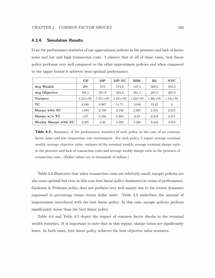
CHAPTER 4. COMMON FACTOR SHOCKS 103
4.3.4. Simulation Results
I run the performance statistics of our approximate policies in the presence and lack of factor
noise and low and high transaction costs. I observe that in all of these cases, best linear
policy performs very well compared to the other approximate policies and when compared
to the upper bound it achieves near-optimal performance.
GP MP MP-TC RBL BL NTC
Avg Wealth 269 573 574.6 547.5 568.5 594.3
Avg Objective 108.1 281.9 282.4 281.1 291.0 297.0
Variance 1.21e+05 1.37e+05 1.37e+05 1.23e+05 1.30e+05 1.44e+05
TC 4.846 9.967 11.71 14.66 13.45 0
Sharpe with TC 1.094 2.188 2.196 2.207 2.231 2.215
Sharpe w/o TC 1.07 2.194 2.204 2.22 2.244 2.215
Weekly Sharpe with TC 2.205 3.39 3.393 3.383 3.443 3.453
Table 4.2: Summary of the performance statistics of each policy in the case of no common
factor noise and low transaction cost environment. For each policy, I report average terminal
wealth, average objective value, variance of the terminal wealth, average terminal sharpe ratio
in the presence and lack of transaction costs and average weekly sharpe ratio in the presence of
transaction costs. (Dollar values are in thousands of dollars.)
Table 4.2 illustrates that when transaction costs are relatively small, myopic policies are
also near-optimal but even in this case best linear policy dominates in terms of performance.
Garleanu & Pedersen policy does not perform very well mainly due to the return dynamics
expressed in percentage terms versus dollar units. Table 4.3 underlines the amount of
improvement introduced with the best linear policy. In this case, myopic policies perform
significantly worse than the best linear policy.
Table 4.4 and Table 4.5 depict the impact of common factor shocks in the terminal
wealth statistics. It is important to note that in this regime, sharpe ratios are significantly
lower. In both cases, best linear policy achieves the best objective value statistics.
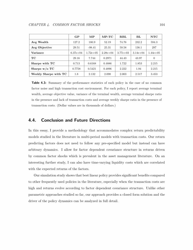
CHAPTER 4. COMMON FACTOR SHOCKS 104
GP MP MP-TC RBL BL NTC
Avg Wealth 127.2 180.9 52.19 74.76 232.2 594.3
Avg Objective 29.51 -98.41 25.31 59.58 138.1 297
Variance 6.37e+04 1.72e+05 2.28e+04 3.77e+03 3.14e+04 1.44e+05
TC 29.16 7.744 0.2971 44.43 43.97 0
Sharpe with TC 0.713 0.6168 0.4886 1.722 1.853 2.215
Sharpe w/o TC 0.7758 0.5421 0.4896 2.222 1.94 2.215
Weekly Sharpe with TC 1.8 2.132 2.098 2.003 2.517 3.453
Table 4.3: Summary of the performance statistics of each policy in the case of no common
factor noise and high transaction cost environment. For each policy, I report average terminal
wealth, average objective value, variance of the terminal wealth, average terminal sharpe ratio
in the presence and lack of transaction costs and average weekly sharpe ratio in the presence of
transaction costs. (Dollar values are in thousands of dollars.)
4.4. Conclusion and Future Directions
In this essay, I provide a methodology that accommodates complex return predictability
models studied in the literature in multi-period models with transaction costs. Our return
predicting factors does not need to follow any pre-specified model but instead can have
arbitrary dynamics. I allow for factor dependent covariance structure in returns driven
by common factor shocks which is prevalent in the asset management literature. On an
interesting further study, I can also have time-varying liquidity costs which are correlated
with the expected returns of the factors.
Our simulation study shows that best linear policy provides significant benefits compared
to other frequently used policies in the literature, especially when the transaction costs are
high and returns evolve according to factor dependent covariance structure. Unlike other
parametric approaches studied so far, our approach provides a closed form solution and the
driver of the policy dynamics can be analyzed in full detail.
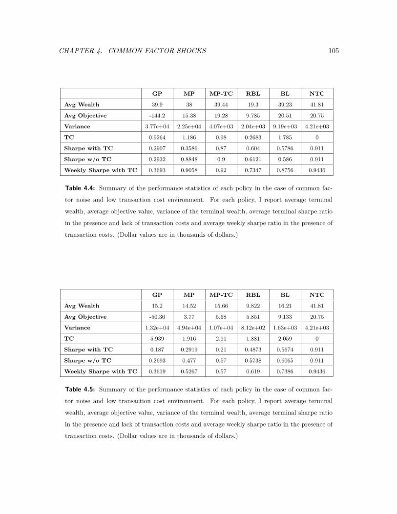
CHAPTER 4. COMMON FACTOR SHOCKS 105
GP MP MP-TC RBL BL NTC
Avg Wealth 39.9 38 39.44 19.3 39.23 41.81
Avg Objective -144.2 15.38 19.28 9.785 20.51 20.75
Variance 3.77e+04 2.25e+04 4.07e+03 2.04e+03 9.19e+03 4.21e+03
TC 0.9264 1.186 0.98 0.2683 1.785 0
Sharpe with TC 0.2907 0.3586 0.87 0.604 0.5786 0.911
Sharpe w/o TC 0.2932 0.8848 0.9 0.6121 0.586 0.911
Weekly Sharpe with TC 0.3693 0.9058 0.92 0.7347 0.8756 0.9436
Table 4.4: Summary of the performance statistics of each policy in the case of common fac-
tor noise and low transaction cost environment. For each policy, I report average terminal
wealth, average objective value, variance of the terminal wealth, average terminal sharpe ratio
in the presence and lack of transaction costs and average weekly sharpe ratio in the presence of
transaction costs. (Dollar values are in thousands of dollars.)
GP MP MP-TC RBL BL NTC
Avg Wealth 15.2 14.52 15.66 9.822 16.21 41.81
Avg Objective -50.36 3.77 5.68 5.851 9.133 20.75
Variance 1.32e+04 4.94e+04 1.07e+04 8.12e+02 1.63e+03 4.21e+03
TC 5.939 1.916 2.91 1.881 2.059 0
Sharpe with TC 0.187 0.2919 0.21 0.4873 0.5674 0.911
Sharpe w/o TC 0.2693 0.477 0.57 0.5738 0.6065 0.911
Weekly Sharpe with TC 0.3619 0.5267 0.57 0.619 0.7386 0.9436
Table 4.5: Summary of the performance statistics of each policy in the case of common fac-
tor noise and low transaction cost environment. For each policy, I report average terminal
wealth, average objective value, variance of the terminal wealth, average terminal sharpe ratio
in the presence and lack of transaction costs and average weekly sharpe ratio in the presence of
transaction costs. (Dollar values are in thousands of dollars.)

BIBLIOGRAPHY 106
Bibliography
Y. Aït-Sahalia and J. Jacod. Is brownian motion necessary to model high-frequency data?
The Annals of Statistics, 38(5):3093–3128, 2010.
Y. Aït-Sahalia and J. Yu. High frequency market microstructure noise estimates and liq-
uidity measures. The Annals of Applied Statistics, 3(1):422–457, 2009.
R. F. Almgren and N. Chriss. Optimal execution of portfolio transactions. Journal of Risk,
3(2):5–39, 2000.
J. Angel. Limit versus market orders. Working Paper No. FINC-1377-01-293, School of
Business Administration, Georgetown University, Washington, D.C., 1994.
J. Bacidore, R. Battalio, and R. Jennings. Order submission strategies, liquidity supply,
and trading in pennies on the New York Stock Exchange. Journal of Financial Markets,
6:337–362, 2003.
K. Back and S. Baruch. Working orders in limit order markets and floor exchanges. The
Journal of Finance, 62(4):1589–1621, 2007.
P. Balduzzi and A. W. Lynch. Transaction costs and predictability: some utility cost
calculations. Journal of Financial Economics, 52(1):47–78, apr 1999.
O.E. Barndorff-Nielsen, D.G. Pollard, and N. Shephard. Discrete-valued levy processes and
low latency financial econometrics. Technical report, Department of Economics (University
of Oxford), 2010.
A. Ben-Tal, A. Goryashko, E. Guslitzer, and A. Nemirovski. Adjustable robust solutions of
uncertain linear programs. Mathematical Programming, 99(2):351–376, 2004.
BIBLIOGRAPHY 107
A. Ben-Tal, B. Golany, A. Nemirovski, and J. Vial. Retailer-supplier flexible commitments
contracts: A robust optimization approach. Manufacturing & Service Operations Man-
agement, 7:248–271, July 2005.
D. P. Bertsekas. Dynamic Programming and Optimal Control. Athena Scientific, 2nd
edition, 2000.
D. Bertsimas and V. Goyal. On the power and limitations of affine policies in two-stage
adaptive optimization. Mathematical Programming, pages 1–41, 2011.
D. Bertsimas and A. Lo. Optimal control of execution costs. Journal of Financial Markets,
1(1):1–50, 1998.
D. Bertsimas, L. Kogan, and A. W. Lo. When is time continuous? Journal of Financial
Economics, 55:173–204, 2000.
D. Bertsimas, D. A. Iancu, and P. A. Parrilo. Optimality of affine policies in multistage
robust optimization. Math. Oper. Res., 35, May 2010.
S. Boyd and L. Vandenberghe. Convex Optimization. Cambridge University Press, March
2004.
S. Boyd, M. T. Mueller, B. O’Donoghue, and Wang Y. Performance bounds and suboptimal
policies for multi-period investment. Working paper, 2012.
P. P. Boyle and D. Emanuel. Discretely adjusted option hedges. Journal of Financial
Economics, 8:259–282, 1980.
M. W. Brandt, P. Santa-Clara, and R. Valkanov. Parametric portfolio policies: Exploit-
ing characteristics in the cross-section of equity returns. Review of Financial Studies,
22(9):3411–3447, September 2009.
Michael W. Brandt, Pedro Santa-Clara, and Rossen Valkanov. Parametric portfolio poli-
cies: Exploiting characteristics in the cross-section of equity returns. Review of Financial
Studies, 22(9):3411–3447, 2009.
BIBLIOGRAPHY 108
J. Brogaard. High frequency trading and its impact on market quality. Working paper,
2010.
D. B. Brown and J. E. Smith. Dynamic portfolio optimization with transaction costs:
Heuristics and dual bounds. Working paper, 2010.
G. C. Calafiore. An affine control method for optimal dynamic asset allocation with trans-
action costs. SIAM J. Control Optim., 48:2254–2274, June 2009.
J.Y. Campbell and L.M. Viceira. Strategic asset allocation. Oxford University Press Oxford,
2002.
G. Cespa and T. Foucault. Insiders-outsiders, transparency, and the value of the ticker.
Working Paper No. 628, Department of Economics, Queen Mary, University of London,
April 2008.
G. C. Chacko, J. W. Jurek, and E. Stafford. The price of immediacy. Journal of Finance,
63(3):1253–1290, 2008.
N. Chen, R. Roll, and S. A. Ross. Economic forces and the stock market. The Journal of
Business, 59(3):pp. 383–403, 1986.
X. Chen, M. Sim, and P. Sun. A robust optimization perspective on stochastic programming.
Operations Research, 55:1058–1071, November 2007.
X. Chen, M. Sim, P. Sun, and J. Zhang. A linear decision-based approximation approach
to stochastic programming. Operations Research, 56:344–357, March 2008.
S.N. Cohen and L. Szpruch. A limit order book model for latency arbitrage. Arxiv preprint
arXiv:1110.4811, 2011.
G.M. Constantinides. Capital market equilibrium with transaction costs. The Journal of
Political Economy, 94(4):pp. 842–862, August 1986.
T. Copeland and D. Galai. Information effects and the bid-ask spread. Journal of Finance,
38(5):1457–1469, 1983.
BIBLIOGRAPHY 109
John C. Cox, Jonathan E. Ingersoll, Jr., and Stephen A. Ross. An intertemporal general
equilibrium model of asset prices. Econometrica, 53:363–384, 1985.
J. Cvitanic and A. Kirilenko. High frequency traders and asset prices. Working paper,
March 2010.
J. Cvitanic. Theory of portfolio optimization in markets with frictions. In E. Jouini,
J. Cvitanic, and Marek Musiela, editors, Handbooks in Mathematical Finance. Cambridge
University Press, 2001.
M. H. A. Davis and A. R. Norman. Portfolio selection with transaction costs. Mathematics
of Operations Research, 15(4):676–713, 1990.
V.V. Desai, V.F. Farias, and C.C. Moallemi. Pathwise optimization for linear convex sys-
tems. Working paper, 2011.
J. B. Detemple, R. Garcia, and M. Rindisbacher. A monte carlo method for optimal port-
folios. The Journal of Finance, 58(1):401–446, February 2003.
Darrell Duffie and Rui Kan. A yield-factor model of interest rates. Mathematical finance,
6(4):379–406, 1996.
B. Dumas and E. Luciano. An exact solution to a dynamic portfolio choice problem under
transactions costs. The Journal of Finance, 46(2):pp. 577–595, 1991.
Bernard Dumas and Elisa Luciano. An exact solution to a dynamic portfolio choice problem
under transactions costs. Journal of Finance, pages 577–595, 1991.
R. Durrett. Probability: Theory and Examples. Duxbury Press, 3rd edition, 2004.
D. Easley, T. Hendershott, and T. Ramadorai. The price of latency. Working paper, May
2008.
E. F. Fama and K. R. French. Multifactor explanations of asset pricing anomalies. The
Journal of Finance, 51(1):pp. 55–84, 1996.
N. Garleanu and L.H. Pedersen. Dynamic trading with predictable returns and transaction
costs. Working paper, April 2012.
BIBLIOGRAPHY 110
J. Gatheral. No-dynamic-arbitrage and market impact. Quantitative Finance, 10(7):749–
759, 2010.
P. Glasserman and X. Xu. Robust portfolio control with stochastic factor dynamics. Work-
ing paper, 2011.
L. R. Glosten. Is the electronic open limit order book inevitable? Journal of Finance,
49(4):1127–1161, 1994.
W. N. Goetzmann and P. Jorion. Testing the predictive power of dividend yields. Journal
of Finance, 48(2):663–679, 1993.
C. Gourieroux, A. Monfort, and E. Renault. Indirect inference. Journal of applied econo-
metrics, 8(S1):S85–S118, 1993.
M. Grant and S. Boyd. CVX: Matlab software for disciplined convex programming, version
1.21. http://cvxr.com/cvx, April 2011.
R. C. Grinold and R. N. Kahn. Active Portfolio Management. McGraw-Hill, 2nd edition,
1999.
S. Grossman and M. Miller. Liquidity and market structure. Journal of Finance, 43:617–
633, 1988.
S.J. Grossman and Z. Zhou. Optimal investment strategies for controlling drawdowns.
Mathematical Finance, 3(3):241–276, 1993.
L. Harris. Optimal dynamic order submission strategies in some stylized trading problems.
Financial Markets, Institutions & Instruments, 7(2):1–76, April 1998.
J. Hasbrouck and G. Saar. Technology and liquidity provision: The blurring of traditional
definitions. Journal of Financial Markets, 12:143–172, 2009.
J. Hasbrouck and G. Saar. Low-latency trading. Working paper, 2010.
J. Hasbrouck. Empirical Market Microstructure. Oxford University Press, 2007.
BIBLIOGRAPHY 111
T. Hendershott and R. Riordan. Algorithmic trading and information. Working paper,
September 2009.
T. Hendershott, C. M. Jones, and A. Menkveld. Does algorithmic trading improve liquidity?
To appear in Journal of Finance, April 2010.
S.L. Heston, R.A. Korajczyk, and R. Sadka. Intraday patterns in the cross-section of stock
returns. Journal of Finance, 65(4):1369–1407, 2010.
M. Hora. Tactical liquidity trading and intraday volume. Working Paper, 2006.
R. A. Jarrow and P. Protter. A dysfunctional role of high frequency trading in electronic
markets. Working paper, 2011.
A. Kirilenko, A. Kyle, M. Samadi, and T. Tuzun. The flash crash: The impact of high
frequency trading on an electronic market. Working paper, 2010.
D. Kuhn, W. Wiesemann, and A. Georghiou. Primal and dual linear decision rules in
stochastic and robust optimization. Mathematical Programming, pages 1–33, 2009.
Ahn Le, Kenneth J. Singleton, and Qiang Dai. Discrete-time affineQ term structure models
with generalized market prices of risk. Review of Financial Studies, 23(5):2184–2227, 2010.
H. Leland. Option pricing and replication with transactions costs. Journal of Finance,
40:1283–1301, 1985.
Han Liu and Mark Loewenstein. Optimal portfolio selection with transaction costs and
finite horizons. Review of Financial Studies, 15(3):805–835, 2002.
H. Liu. Optimal consumption and investment with transaction costs and multiple risky
assets. Journal of Finance, 59(1):289–338, 02 2004.
A. W. Lo, A. C. MacKinlay, and J. Zhang. Econometric models of limit order execution.
Journal of Financial Economics, 65:31–71, 2002.
A. W. Lynch and P. Balduzzi. Predictability and transaction costs: The impact on rebal-
ancing rules and behavior. Journal of Finance, 55(5):2285–2309, October 2000.
BIBLIOGRAPHY 112
A. W. Lynch and S. Tan. Multiple risky assets, transaction costs, and return predictability:
Allocation rules and implications for u.s. investors. Journal of Financial and Quantitative
Analysis, 45(04):1015–1053, August 2010.
Robert C. Merton. Optimum consumption and portfolio rules in a continuous-time model.
Journal of Economic Theory, 3(4):373–413, December 1971.
A. Nemirovski, A. Juditsky, G. Lan, and A. Shapiro. Stochastic approximation approach
to stochastic programming. SIAM Journal on Optimization, 19(4):1574–1609, 2009.
A. A. Obizhaeva and J. Wang. Optimal trading strategy and supply/demand dynamics.
Working paper, 2005.
E. Pagnotta. Information and liquidity trading at optimal frequencies. Technical report,
Working paper, NYU Stern, 2010.
C.A. Parlour and D.J. Seppi. Limit order markets: A survey. Handbook of Financial
Intermediation and Banking, 5, 2008.
A. F. Perold. The implementation shortfall: Paper versus reality. Journal of Portfolio
Management, 14(3):4–9, 1988.
M. J. Ready. The specialist’s discretion: Stopped orders and price improvement. Review of
Financial Studies, 12(5):1075–112, Winter 1999.
R. Roll. A simple implicit measure of the effective bid-ask spread in an efficient market.
Journal of Finance, 39:1127–1139, 1984.
P. Sandås. Adverse selection and competitive market making: Empirical evidence from a
limit order market. Review of Financial Studies, 14(3):705–734, 2001.
A. Shapiro and A. Nemirovski. On complexity of stochastic programming problems. Con-
tinuous optimization, pages 111–146, 2005.
A. Shapiro. Monte carlo sampling methods. In A. Ruszczynski and A. Shapiro, editors,
Stochastic Programming, volume 10 of Handbooks in Operations Research and Manage-
ment Science, pages 353 – 425. Elsevier, 2003.
BIBLIOGRAPHY 113
S. E. Shreve and H. M. Soner. Optimal investment and consumption with transaction costs.
The Annals of Applied Probability, 4(3):pp. 609–692, 1994.
J. Skaf and S.P. Boyd. Design of affine controllers via convex optimization. Automatic
Control, IEEE Transactions on, 55(11):2476 –2487, November 2010.
H. R. Stoll and C. Schenzler. Trades outside the quotes: Reporting delay, trading option
or trade size? Journal of Financial Economics, 79:615–653, 2006.
Oldrich A. Vasicek. An equilibrium characterization of the term structure. Journal of
Financial Economics, 5(2):177–188, 1977.
I. Werner. NYSE order flow, spreads, and information. Journal of Financial Markets,
6:309–335, 2003.
APPENDIX A. THE COST OF LATENCY 114
Appendix A
The Cost of Latency
A.1. Dynamic Programming Decomposition
In order to solve the optimal control problem (2.8) via dynamic programming, note that we
can equivalently consider the objective of maximizing the sale price P . Consider a decision
time Ti with 0 ≤ i < n, and assume that the trader’s limit order remains unfilled at time Ti.
The state of the system consists of the current price, STi as well as the previously chosen
limit price,1 `i−1, since this price will become active at time Ti. We can define an optimal
value function Ji(STi , `i−1), as a function of this state, by optimizing the eventual sale price
over all future decisions. In other words,
(A.1) Ji(STi , `i−1) , maximize`i,...,`n−1
E [P | STi , `i−1] .
At time T = Tn, the trader must sell via a market order, hence
(A.2) Jn(STn , `n−1) = STn .
Now, for 0 ≤ i < n, there are three mutually exclusive events one of which must
occur between time Ti and time Ti+1. These are the events E(1)i , E(2)
i , and E(3)i described
in Section 4.2. By considering cases corresponding to these events, we have the Bellman
equation
(A.3) Ji(STi , `i−1) , max`i
E[IE(1)i
`i−1 + IE(2)i
STi+1 + IE(3)i
Ji+1(STi+1 , `i)∣∣∣∣ STi , `i−1
].
1I will assume that `−1 =∞, i.e., there is no limit order active at the beginning of the time horizon.
APPENDIX A. THE COST OF LATENCY 115
Here, the first term corresponds to an execution at the prior price `i−1, the second term
corresponds to the price `i being crossed by the bid price upon arrival to the market, and
the third term corresponds to all other cases.
Define the function Qi, for 0 ≤ i ≤ n, by
Qi(STi , vi−1) , Ji(STi , STi + vi−1)− STi .
The function Qi is the premium of the value at time Ti, relative to the current bid price
STi . Similarly, vi−1 , `i−1 − STi is the premium of limit price decided at time Ti−1 relative
to the current bid price at time Ti. Then, applying (A.3), we have for 0 ≤ i < n,
Qi(STi , vi−1)
= max`i
E[IE(1)i
(STi + vi−1) + IE(2)i
STi+1 + IE(3)i
Ji+1(STi+1 , `i)∣∣∣∣ STi , vi−1
]− STi
= maxui
E[IE(1)i
vi−1 + IE(2)i ∪E
(3)i
Xi+1 + IE(3)i
Qi+1(STi +Xi+1, ui −Xi+1)∣∣∣∣ STi , vi−1
].
Here, Xi+1 , STi+1−STi ∼ N(0, σ2∆t) is the change in bid price from time Ti to time Ti+1.
I define ui , `i−STi as the premium of the limit price at time Ti (i.e., the decision variable)
relative to the current bid price STi . Note that the price change Xi+1 is zero mean under
the event
E(2)i ∪ E
(3)i =
(E(1)i
)c,
by the assumption that the arrival of impatient buyers is independent of the bid price
process, hence
(A.4) Qi(STi , vi−1) = maxui
E[IE(1)i
vi−1 + IE(3)i
Qi+1(STi +Xi+1, ui −Xi+1)∣∣∣∣ STi , vi−1
].
Finally, by (A.2),
(A.5) Qn(STn , vn−1) = 0.
As should be clear from the above discussion, the Bellman equation (A.3) with terminal
condition (A.2) and the backward recursion (A.4) with terminal condition (A.5) are com-
pletely equivalent, up to a change in variables. Expressing these equations in the latter
form, however, brings significant simplifications, as the following lemma shows.
APPENDIX A. THE COST OF LATENCY 116
Lemma 4. Suppose a collection of functions Qi satisfies the dynamic programming equa-
tions (A.4)–(A.5). Then, for each 0 ≤ i < n, Qi does not depend on the price STi, and
takes the form
(A.6) Qi(vi−1) = Ivi−1≤δ [µ∆tvi−1 + (1− µ∆t)hi ] + Ivi−1>δhi,
where the scalar hi satisfies
(A.7) hi = maxui
P(Xi+1 < ui)E [Qi+1(ui −Xi+1) | Xi+1 < ui] .
Proof. Observe that, for 0 ≤ i < n, (A.4) can be simplified according to
Qi(STi , vi−1)
= maxui
µ∆tvi−1Ivi−1≤δ
+(1− µ∆tvi−1Ivi−1≤δ
)E[IXi+1<uiQi+1(STi +Xi+1, ui −Xi+1)
∣∣∣ STi] ,
(A.8)
where I have used the definitions of the events E(1)i and and E(3)
i .
Now, we proceed by backward induction. For the terminal case i = n − 1, from (A.8)
and the fact that Qn = 0 and un−1 = −∞ (i.e., the trader must use a market order at the
last time slot), we have that
Qn−1(STn−1 , vn−2) = µ∆tvn−2Ivn−2≤δ.
In other words, Qn−1 satisfies the hypotheses of the lemma, with hn−1 = 0.
Now, suppose that the result holds for some 0 ≤ i + 1 < n. By (A.8), and since Qi+1
does not depend on STi+1 ,
Qi(STi , vi−1)
= maxui
µ∆tvi−1Ivi−1≤δ +(1− µ∆tvi−1Ivi−1≤δ
)E[IXi+1<uiQi+1(ui −Xi+1)
]= µ∆tvi−1Ivi−1≤δ +
(1− µ∆tvi−1Ivi−1≤δ
)hi
= Ivi−1≤δ [µ∆tvi−1 + (1− µ∆tvi−1)hi ] + Ivi−1>δhi.
Here, in the second equality, I define hi through (A.7). The result then follows.
APPENDIX A. THE COST OF LATENCY 117
Notice that, at the beginning of the trading horizon, there is no active limit order, i.e.,
u−1 =∞. From Lemma 4, I have that
h0 = Q0(∞) = maximize`0,...,`n−1
E [P | S0]− S0.
In other words, h0 = h0(∆t), as defined in (2.8), and the notation is consistent. More
generally, for i > 0, from (A.7), I can interpret hi to be the trader’s expected payoff at time
Ti relative to the current bid price under the optimal policy, assuming that the limit order
does not get executed in that time slot. Thus, hi can be interpreted as a continuation value
in the dynamic programming context, as in (2.9).
The continuation values hi allow for a compact representation of the value function,
since they consist of only a single real number for each time slot, rather than a function of
the entire state space. Theorem 1 directly expresses the dynamic programming equations
(A.4)–(A.5) in terms of this representation. The proof follows by explicitly computing the
expectations in Lemma 4.
Theorem 1. Suppose hi satisfy, for 0 ≤ i < n− 1,
hi = maxui
µ∆t
[ui
(Φ(
ui
σ√
∆t
)− Φ
(ui − δσ√
∆t
))+ σ√
∆t(φ
(ui
σ√
∆t
)− φ
(ui − δσ√
∆t
))]+hi+1
[(1− µ∆t)Φ
(ui
σ√
∆t
)+ µ∆tΦ
(ui − δσ√
∆t
)],
(A.9)
and
(A.10) hn−1 = 0.
Here, φ and Φ are, respectively, the p.d.f. and c.d.f. of the standard normal distribution.
Then, hi correspond to the continuation values under the optimal policy. In other words,
the value functions Qi defined by hi via (A.6) solve the dynamic programming equations
(A.4)–(A.5).
Suppose further that, for 0 ≤ i < n − 1, u∗i is a maximizer of (A.9). Then, a policy
which chooses limit prices according to the premia defined by u∗i , i.e.,
`∗i = STi + u∗i , ∀ 0 ≤ i < n− 1,
is optimal.
APPENDIX A. THE COST OF LATENCY 118
Proof. Suppose that I am given hi that satisfy the hypotheses of the theorem. Define
Qi by setting, for 0 ≤ i ≤ n− 1,
(A.11) Qi(vi−1) , Ivi−1≤δ [µ∆tvi−1 + (1− µ∆t)hi ] + Ivi−1>δhi,
and Qn , 0. I wish to show that Qi solve the dynamic programming equations (A.4)–
(A.5).
Note that (A.5) holds by definition. For 0 ≤ i < n, we have that (A.4) is equivalent to
(A.8). Define Qi to be the right side of (A.8), i.e.,
Qi(vi−1) , µ∆tvi−1Ivi−1≤δ +(1− µ∆tvi−1Ivi−1≤δ
)maxui
E[IXi+1<uiQi+1(ui −Xi+1)
].
Comparing with (A.11), in order that the dynamic programming equation (A.8) hold (i.e.,
that Qi = Qi), we must have that
(A.12) hi = maxui
E[IXi+1<uiQi+1(ui −Xi+1)
]Using the definition of Qi+1 from (A.11), this is equivalent to
hi
= maxui
E[IXi+1<ui
(Iui−Xi+1≤δ [µ∆t(ui −Xi+1) + (1− µ∆t)hi+1 ] + Iui−Xi+1>δhi+1
)]= max
uiE[I0<ui−Xi+1≤δµ∆t(ui −Xi+1) + IXi+1<ui(1− µ∆t)hi+1 + Iui−Xi+1>δµ∆thi+1
].
For the first term in the expectation, we have
E[I0<ui−Xi+1≤δµ∆t(ui −Xi+1)
]= µ∆t
∫ ui
−∞(ui − x)Iui−x≤δ
1σ√
∆tφ
(x
σ√
∆t
)dx
= µ∆t∫ ui
ui−δ(ui − x) 1
σ√
∆tφ
(x
σ√
∆t
)dx
= µ∆t[ui
(Φ(
ui
σ√
∆t
)− Φ
(ui − δσ√
∆t
))+∫ ui
ui−δ
−xσ√
∆tφ
(x
σ√
∆t
)dx
]= µ∆t
[ui
(Φ(
ui
σ√
∆t
)− Φ
(ui − δσ√
∆t
))+ σ√
∆t(φ
(ui
σ√
∆t
)− φ
(ui − δσ√
∆t
))].
For the second term in the expectation, we have
E[IXi+1<ui(1− µ∆t)hi+1
]= (1− µ∆t)hi+1Φ
(ui
σ√
∆t
).
APPENDIX A. THE COST OF LATENCY 119
finally, for the last term in the expectation, we have
E[Iui−Xi+1>δµ∆thi+1
]= µ∆thi+1Φ
(ui − δσ√
∆t
)Combining all the terms, I obtain the desired recursion for hi.
The balance of the theorem (i.e., the optimality of the u∗i policy) follows from standard
dynamic programming arguments.
A.2. Proof of Theorem 2
I begin with a preliminary lemma.
Lemma 5. Suppose that hi : 0 ≤ i < n solves the dynamic programming recursion
(2.10)–(2.11). Then, for 0 ≤ i < n,
(A.13) 0 ≤ hi ≤ δ (1− (1− µ∆t)n ) < δ.
Proof. First, note that the result is trivially true for i = n − 1, since hn−1 = 0. Now, if
0 ≤ i < n − 1, we can always choose ui = −∞, i.e., a market order, and this results in a
continuation value of 0. Thus, hi ≥ 0.
For the upper bound, consider the discrete model without latency described in Sec-
tion 2.4.3. Any strategy for the latency model is also feasible for the discrete model, since
the trader can simply delay the implementation of trading decisions by one period. There-
fore, at time Ti (with 0 ≤ i < n− 1), a policy with latency cannot achieve more value than
the optimal policy for the discrete model without latency. At time Ti, there are n − i − 1
trading decisions remaining. This corresponds to the initial time of a discrete model with
a total time horizon of (n− i− 1)∆t. Then, with reference to Lemma 2, we have that
hi ≤ δ (1− (1− µ∆t)n−i−1 ).
The result immediately follows.
Theorem 2. Fix α > 1. If ∆t is sufficiently small, then there exists a unique optimal solution
hi to the dynamic programming equations (2.10)–(2.11). Moreover, the corresponding
APPENDIX A. THE COST OF LATENCY 120
optimal policy u∗i is unique. For 0 ≤ i < n − 1, this strategy chooses limit prices in the
range
`∗i ∈
Si + δ − σ
√∆t log αL∆t , Si + δ − σ
√∆t log R(∆t)
∆t ,
,where
L ,δ2
2πσ2 , R(∆t) , δ2(1− µ∆t)2n
2πσ2 .
Proof. Assume that, for some 0 ≤ i < n − 1, a solution hj : i + 1 ≤ j < n exists to
(2.10)–(2.11). I will establish that, for ∆t sufficiently small (and not dependent on i), a
solution hi also exists and satisfies the conditions of the theorem. The result will follow by
backward induction. Note that the base case of the induction (i.e., the existence of hn−1)
is trivial.
To this end, define the auxiliary function f by
f(u, h) , µ∆t[u(Φ(Au)− Φ(Bu)) + σ
√∆t(φ(Au)− φ(Bu))
]+ h
[(1− µ∆t)Φ(Au) + µ∆tΦ(Bu)
],
(A.14)
where
Au ,u
σ√
∆t, Bu ,
u− δσ√
∆t.(A.15)
Then, from Theorem 1, for 0 ≤ i < n− 1, the dynamic programming recursion is given by
(A.16) hi = maxui
f(ui, hi+1),
and I can establish the present theorem by proving that, for ∆t sufficiently small, (A.16)
has a unique maximizer u∗i ∈ (uL, uR), where
uL , δ − σ
√∆t log αL∆t , uR , δ − σ
√∆t log R(∆t)
∆t .(A.17)
Note that
(A.18) R(0) , lim∆t→0
R(∆t) = lim∆t→0
L(1− µ∆t)2T/dt = Le−2µT < αL.
Hence, there exists some ∆t > 0 so that if 0 < ∆t < ∆t, then
δ/2 < uL < uR < δ, and 0 < 1− µ∆t < 1.

APPENDIX A. THE COST OF LATENCY 121
For the balance of the theorem, I will assume that 0 < ∆t < ∆t, in addition to whatever
other assumptions are made regarding the magnitude of ∆t.
The first and second derivatives of f(·, h) are given by
fu(u, h) = µ∆t[Φ(Au)− Φ(Bu) +Au (φ(Au)− φ(Bu))− uφ(Au) + (δ − u)φ(Bu)
σ√
∆t
]+ h
σ√
∆t
[(1− µ∆t)φ(Au) + µ∆tφ(Bu)
]= (1− µ∆t)h
σ√
∆tφ(Au) + µ∆t
[Φ(Au)− Φ(Bu)− δ
σ√
∆tφ(Bu)
]+ hµ
√∆t
σφ(Bu)
= (1− µ∆t)hσ√
∆tφ(Au) + µ∆t[Φ(Au)− Φ(Bu)] + µ
√∆tσ
φ(Bu)(h− δ),
fuu(u, h) = −u(1− µ∆t)hσ3∆t
√∆t
φ(Au) + µ√
∆tσ
[φ(Au)− φ(Bu)] + µ(δ − u)σ3√
∆tφ(Bu)(h− δ)
= φ(Au)[µ√
∆tσ− u(1− µ∆t)h
σ3∆t3/2
]+ φ(Bu)
[µ(δ − u)σ3√
∆t(h− δ)− µ
√∆tσ
].
(A.19)
First, I will show that, for ∆t sufficiently small, f(·, hi+1) has a local maximum u∗i in
the interval (uL, uR), and that this is the unique maximizer over the larger interval (δ/2, δ).
That is, u ∈ (δ/2, δ) and u 6= u∗i , then
(A.20) f(u, hi+1) < f(u∗i , hi+1), for all u ∈ (δ/2, δ), u 6= u∗i .
This is implied by the following claims, which I will demonstrate hold for ∆t sufficiently
small:
(i) fu(uL, hi+1) > 0.
(ii) fu(uR, hi+1) < 0.
(iii) fuu(u, hi+1) < 0, for all u ∈ (δ/2, δ).
Claim (i): Note that
fu(uL, hi+1) = (1− µ∆t)hi+1
σ√
∆tφ(AuL) + µ∆t[Φ(AuL)− Φ(BuL)] + µ∆t
δ√α
(hi+1 − δ)
≥ µ∆t[Φ(AuL)− Φ(BuL)]− µ∆t√α,
(A.21)
APPENDIX A. THE COST OF LATENCY 122
where I use the fact that hi+1 ≥ 0 (cf. Lemma 5). In order to calculate a lower bound
for Φ(AuL) − Φ(BuL), we need the following standard bound on the tail probabilities of
the normal distribution [see, e.g., Durrett, 2004]. Define Q to be the tail probability of a
standard normal distribution, i.e.,
Q(x) , 1− Φ(x) = 1√2π
∫ ∞x
e−12u
2du.
Then, for all x > 0,
(A.22) x2 − 1x3√
2πe−
12x
2≤ Q(x) ≤ 1
x√
2πe−
12x
2.
Applying this to (A.21),
fu(uL, hi+1) ≥ µ∆t[1−Q(AuL)−Q(−BuL)
]+ µ∆t√
α
= µ∆t(
1− 1√α
)− µ∆t[Q(AuL) +Q(−BuL)]
> µ∆t(
1− 1√α
)− 2µ∆tQ(−BuL)
≥ µ∆t(
1− 1√α
)− 2µ∆t3/2√
2παL log αL∆t
> 0,
for sufficiently small ∆t. Here, I have used the fact that Q(−BuL) > Q(AuL).
Claim (ii): Similarly, for the other endpoint of the interval, I have
fu(uR, hi+1) = (1− µ∆t)hi+1
σ√
∆tφ(AuR) + µ∆t[1−Q(AuR)−Q(−BuR)]
+ µ∆tδ(1− µ∆t)n (hi+1 − δ)
≤ (1− µ∆t)hi+1
σ√
∆tφ(AuR) + µ∆t[1−Q(AuR)−Q(−BuR)]
+ µ∆tδ(1− µ∆t)n [δ (1− (1− µ∆t)n)− δ]
= (1− µ∆t)hi+1
σ√
∆tφ(AuR) + µ∆t[1−Q(AuR)−Q(−BuR)]− µ∆t
= (1− µ∆t)hi+1
σ√
∆tφ(AuR)− µ∆t[Q(AuR) +Q(−BuR)]
≤ δ
σ√
∆tφ(AuR)− µ∆tQ(−BuR),

APPENDIX A. THE COST OF LATENCY 123
where I have used the upper bound on hi+1 from Lemma 5. Using (A.18), for sufficiently
small ∆t, I have √log R(∆t)
∆t <δ
2σ√
∆t,
and thus
AuR ≥δ
2σ√
∆t.
On the other hand, using (A.22),
Q(−BuR) ≥[(
log R(∆t)∆t
)−1/2−(
log R(∆t)∆t
)−3/2]√ ∆t2πR(∆t) .
Thus,
fu(uR, hi+1) ≤ δ
σ√
2π∆texp
(−δ2
8σ2∆t
)
− µ∆t[(
log R(∆t)∆t
)−1/2−(
log R(∆t)∆t
)−3/2]√ ∆t2πR(∆t)
< 0,
for sufficiently small ∆t.
Claim (iii): Note that, for u ∈ (δ/2, δ),
φ
(δ
σ√
∆t
)< φ(Au) < φ
(δ
2σ√
∆t
)< φ(Bu) < φ(0).
Then, from (A.19), and using the fact that 0 ≤ hi+1 < δ (cf. Lemma 5), I have for ∆t
sufficiently small,
fuu(u, hi+1) ≤ φ(Au)µ√
∆tσ
+ φ(Bu)[µ(δ − u)σ3√
∆t(hi+1 − δ)−
µ√
∆tσ
]
≤ φ(Bu)µ(δ − u)σ3√
∆t(hi+1 − δ) < 0.
In order to complete the proof, it suffices to demonstrate that the local maximum u∗i ∈
(uL, uR) is the unique global maximum. Since u∗i achieves a higher value than any other
u ∈ (δ/2, δ), I will analyze cases where u /∈ (δ/2, δ) as follows:
• u ∈ [0, δ/2].

APPENDIX A. THE COST OF LATENCY 124
Here,
φ
(δ
σ√
∆t
)≤ φ(Bu) ≤ φ
(δ
2σ√
∆t
)≤ φ(Au) ≤ φ(0).
Further, for ∆t sufficiently small,
Φ(Au)− Φ(Bu) ≥ Φ (0)− Φ( −δ
2σ√
∆t
)≥ 1
4 .
Then, for ∆t sufficiently small,
fu(u, hi+1) ≥ (1− µ∆t)hi+1
σ√
∆tφ
(δ
2σ√
∆t
)+ µ∆t
[Φ (0)− Φ
( −δ2σ√
∆t
)]+ µ√
∆tσ
φ
(δ
2σ√
∆t
)(hi+1 − δ)
≥ hi+1
σ√
∆tφ
(δ
2σ√
∆t
)+ µ∆t
[Φ (0)− Φ
( −δ2σ√
∆t
)]− δµ
√∆t
σφ
(δ
2σ√
∆t
)≥ µ∆t
4 − µδ√
∆t√2πσ
exp(−δ2
8σ2∆t
)> 0.
(A.23)
Here, I have used the fact that hi+1 ≥ 0. Using (A.20) and the fact that f(·, hi+1) is
continuous, this implies that
(A.24) supu∈[0,δ/2]
f(u, hi+1) ≤ f(δ/2, hi+1) < f(u∗i , hi+1).
• u ∈ (−∞, 0).
In this case, since hi+1 ≥ 0 and Bu < Au < 0,
fu(u, hi+1) ≥ µ∆t [Φ(Au)− Φ(Bu)]− δµ√
∆tσ
φ(Bu)
= µ∆t∫ Au
Buφ(z) dz − δµ
√∆t
σφ(Bu)
> µ∆t(Au −Bu)φ(Bu)− δµ√
∆tσ
φ(Bu) = 0.
In conjunction with (A.24), this implies that
(A.25) supu∈(−∞,0)
f(u, hi+1) ≤ f(0, hi+1) < f(u∗i , hi+1).

APPENDIX A. THE COST OF LATENCY 125
• u ∈ [δ,∞).
In this case, using the upper bound on hi+1 from Lemma 5,
fu(u, hi+1) ≤ δ
σ√
∆tφ(Au) + µ∆t [Φ(Au)− Φ(Bu)]
− µδ(1− µ∆t)n√
∆tσ
φ(Bu).(A.26)
Consider two cases. First, assume that u > δ +√
∆t. Then, applying (A.22),
fu(u, hi+1) ≤ δ
σ√
∆tφ(Au) + µ∆tQ(Bu)− µδ(1− µ∆t)n
√∆t
σφ(Bu)
≤ δ
σ√
∆tφ(Au) + µσ∆t3/2
u− δφ(Bu)− µδ(1− µ∆t)n
√∆t
σφ(Bu)
≤ φ(Bu)[
δ
σ√
∆texp
(−δ2
2σ2∆t
)+ µσ∆t− µδ(1− µ∆t)n
√∆t
σ
].
Note that (1− µ∆t)n → e−µT as ∆t→ 0. Then, for ∆t sufficiently small,
(A.27) 12e−µT < (1− µ∆t)n.
Hence, for ∆t sufficiently small,
fu(u, hi+1) ≤ φ(Bu)[
δ
σ√
∆texp
(−δ2
2σ2∆t
)+ µσ∆t− µδe−µT
√∆t
2σ
]< 0.
On the other hand, suppose that u ∈ [δ, δ +√
∆t]. Then, from (A.26), (A.27), and
since 0 < Bu < Au, I have for ∆t sufficiently small,
fu(u, hi+1) ≤ δ
σ√
∆tφ(Au) + µ∆t
2 − µδ(1− µ∆t)n√
∆tσ
φ(Bu)
≤ δ
σ√
∆tφ(Au) + µ∆t
2 − µδe−µT√
∆t2σ φ(Bu)
≤ δ
σ√
2π∆texp
(− δ2
2σ2∆t
)+ µ∆t
2 − µδe−µT√
∆t2σ√
2πexp
(− 1
2σ2
)< 0.
The above discussion, combined with (A.20) and the fact that f(·, hi+1) is continuous,
implies that
(A.28) supu∈[δ,∞)
f(u, hi+1) ≤ f(δ, hi+1) < f(u∗i , hi+1).

APPENDIX A. THE COST OF LATENCY 126
A.3. Proof of Theorem 3
I will establish Theorem 3 via a sequence of lemmas. First, recall the function f(u, h)
defined in (A.14) and the quantities uL and uR defined in (A.17).
Lemma 6. (i) As ∆t→ 0,
maxu∈[uL,uR]0≤i<n−1
|fuu(u, hi+1)| = O
(√∆t log 1
∆t
).
(ii) For all h ∈ R and ∆t sufficiently small,
0 ≤ fh(uR, h) ≤ 1.
Proof. I begin with (i). Recall Au and Bu from (A.15). Let u be in the interval [uL, uR].
Then, for 0 ≤ i < n− 1, from (A.19),
|fuu(u, hi+1)| ≤∣∣∣∣∣φ(Au)
[µ√
∆tσ− u(1− µ∆t)hi+1
σ3∆t3/2
]+ φ(Bu)
[µ(δ − u)σ3√
∆t(hi+1 − δ)−
µ√
∆tσ
]∣∣∣∣∣≤ φ(Au)µ
√∆tσ
+ φ(Au) δ2
σ3∆t3/2+ φ
(δ − uσ√
∆t
)[δµ(δ − u)σ3√
∆t+ µ√
∆tσ
].
Here, I have used the fact that 0 ≤ u ≤ δ and 0 ≤ hi+1 < δ (cf. Lemma 5). Note that, for
∆t sufficiently small, uL ≥ δ/2. Then,
maxu∈[uL,uR]
φ(Au) ≤ φ(Aδ/2) = 1√2π
exp(− δ2
8σ2∆t
)≤ c0∆t2,
for an appropriately chosen constant c0. Thus,
|fuu(u, hi+1)| ≤ c0µ
σ∆t5/4 + c0δ
2
σ3
√∆t+ φ
(δ − uσ√
∆t
)[δµ(δ − u)σ3√
∆t+ µ√
∆tσ
]
≤ c0µ
σ∆t5/4 + c0δ
2
σ3
√∆t+ φ
(δ − uRσ√
∆t
)[δµ(δ − uL)σ3√
∆t+ µ√
∆tσ
]
= c0µ
σ∆t5/4 + c0δ
2
σ3
√∆t+
√∆t
2πR(∆t)
δµσ2
√log αL∆t + µ
√∆tσ
≤ c0µ
σ∆t5/4 + c0δ
2
σ3
√∆t+ µ∆t
σ√
2πR(∆t)+ δµ
σ2√
2πR(∆t)
√∆t log αL∆t .
Since R(∆t)→ Le−2µT as ∆t→ 0, the last term asymptotically dominates and (i) follows.
APPENDIX A. THE COST OF LATENCY 127
For (ii), note that Φ(AuR),Φ(BuR) ∈ (0, 1), so if ∆t < 1/µ, then for all h,
fh(uR, h) = (1− µ∆t)Φ(AuR) + µ∆tΦ(BuR) ∈ (0, 1).
Lemma 7. As ∆t→ 0,
uR − uL = O
(√∆t
log 1∆t
).
Proof. Note that
uR − uL = σ√
∆t
√log αL∆t −
√log R(∆t)
∆t
= σ√
∆t[g(αL)− g(R(∆t))
],
where g(x) ,√
log x∆t . Then, by mean value theorem, for some z ∈ [R(∆t), αL],
uR − uL = σ√
∆tg′(z)[αL−R(∆t)] = σ
2z [αL−R(∆t)]√
∆tlog z
∆t≤ σαL
2R(∆t)
√√√√ ∆tlog R(∆t)
∆t.
The result follows since R(∆t)→ R(0) , Le−2µT as ∆t→ 0.
Let hi : 0 ≤ i < n−1 be the optimal solution to the dynamic programming recursion
(2.10)–(2.11), and let u∗i : 0 ≤ i < n− 1 define the corresponding optimal policy. Define
hi : 0 ≤ i ≤ n− 1 by the recursion
hi ,
f(uR, hi+1) if 0 ≤ i < n− 1,
0 if i = n− 1.
Note that hi is the continuation value of the suboptimal policy that always chooses ui = uR,
for 0 ≤ i < n− 1. I am interested in quantifying its difference to the optimal continuation
value.
Lemma 8. As ∆t→ 0,
0 ≤ h0 − h0 = O
(√∆t
log 1∆t
).
Proof. For 0 ≤ i < n− 1, define ∆i , hi − hi. Clearly, ∆i ≥ 0.

APPENDIX A. THE COST OF LATENCY 128
Using the mean value theorem,
∆i = f(u∗i , hi+1)− f(uR, hi+1)
=[f(u∗i , hi+1)− f(uR, hi+1)
]+[f(uR, hi+1)− f(uR, hi+1)
]= −1
2fuu(u, hi+1)(uR − u∗i )2 + fh(uR, h)∆i+1.
where u is some point on the interval (u∗i , uR) and h is some point on the interval (hi+1, hi+1).
Here, I have used the fact that the optimal solution u∗i satisfies the first order condition
fu(u∗i , hi+1) = 0.
Using Lemmas 6 and 7, for ∆t sufficiently small, there exist constants c1 and c2 so that
maxu∈[uL,uR]0≤i<n−1
|fuu(u, hi+1)| ≤ c1
√∆t log 1
∆t , uR − uL ≤ c2
√∆t
log 1∆t.
Also, from Lemma 6, note that 0 ≤ fh(uR, h) ≤ 1. Then, I obtain that, for ∆t sufficiently
small,
∆i ≤c1(uR − u∗i )2
2
√∆t log 1
∆t + ∆i+1 ≤c1c2
2∆t3/2√log 1
∆t
+ ∆i+1.
Then, since ∆n−1 = 0, I have that
∆0 ≤(T
∆t
)c1c2
2∆t3/2√log 1
∆t
= c1c2T
2
√∆t
log 1∆t.
Define the sequence βi : 0 ≤ i ≤ n− 1 by the linear recursion
(A.29) βi ,
µ∆t(uR − βi+1) + βi+1 if 0 ≤ i < n− 1,
0 if i = n− 1.
Here, βi is an approximation to the value hi. The next lemma bounds the approximation
error.
Lemma 9. As ∆t→ 0,
|h0 − β0| = O
(√∆t
log 1∆t
).
APPENDIX A. THE COST OF LATENCY 129
Proof. For 0 ≤ i < n− 1, define εi , hi− βi. Recall the following definition from the proof
of Theorem 2,
AuR ,uR
σ√
∆t, BuR ,
uR − δσ√
∆t= −
√log R(∆t)
∆t .
Then, by the recursive definitions of hi and βi, 0 ≤ i < n− 1,
εi = (1− µ∆t)εi+1 − µ∆tuR [1− Φ(AuR) + Φ(BuR)] + µσ∆t3/2 [φ(AuR)− φ(BuR)]
− (1− µ∆t)hi+1
[1− Φ(AuR)− µ∆t
1− µ∆tΦ(BuR)].
Since µR is not the optimal policy, I have hi+1 ≤ hi+1 < δ (cf. Lemma 5). Further, for ∆t
sufficiently small, 0 < φ(AuR) ≤ φ(BuR). This implies that
|εi| ≤ (1− µ∆t)|εi+1|+ δµ∆t[1− Φ(AuR) + Φ(BuR)] + µσ∆t3/2φ(BuR)
+ δ
[1− Φ(AuR) + µ∆t
1− µ∆tΦ(BuR)].
Note that, except for the first term, there is no dependence on i in the right side of this
equality. Then, I can define
C(∆t) , δµ∆t[1− Φ(AuR) + Φ(BuR)] + µσ∆t3/2φ(BuR)
+ δ
[1− Φ(AuR) + µ∆t
1− µ∆tΦ(BuR)],
and I have that
|εi| ≤ (1− µ∆t)|εi+1|+ C(∆t).
Since εn−1 = 0, it is easy to verify by backward induction on i that
|εi| ≤1− (1− µ∆t)n−i−1
µ∆t C(∆t).
Therefore,
|ε0| ≤1− (1− µ∆t)n−1
µ∆t C(∆t) ≤ C(∆t)µ∆t
= δ [1− Φ(AuR) + Φ(BuR)] + µσ√
∆tφ(BuR) + δ
µ∆t
[1− Φ(AuR) + µ∆t
1− µ∆tΦ(BuR)]
= δ [Q(AuR) +Q(−BuR)] + µσ√
∆tφ(BuR) + δ
µ∆t
[Q(AuR) + µ∆t
1− µ∆tQ(−BuR)].
(A.30)

APPENDIX A. THE COST OF LATENCY 130
From (A.22), however,
Q(AuR) ≤ σ
uR
√∆t2π exp
(− u2
R
2σ∆t
).
Since uR → δ as ∆t → 0, for ∆t sufficiently small, there exists constants a1 and a2, with
0 < a2 < δ2/2σ, so that
Q(AuR) ≤ a1√
∆t exp(− a2
∆t
).
Also by (A.22),
Q(−BuR) ≤
√√√√ ∆t2πR(∆t) log R(∆t)
∆t.
Since and R(∆t) → R(0) , Le−2µT as ∆t → 0, for ∆t sufficiently small, there exists a
constant a3 so that
Q(−BuR) ≤ a3
√∆t
log 1∆t.
Finally,
φ(BuR) =√
∆t2πR(∆t) ,
so for ∆t sufficiently small, there exists a constant a4 with
φ(BuR) ≤ a4√
∆t.
Applying these bounds to (A.30), the result follows.
Lemma 10. As ∆t→ 0,
β0 = uR(1− e−µT
)+O(∆t).
Proof. Note that the recurrence (A.29) can be explicitly solved to obtain
β0 =n−2∑i=0
(1− µ∆t)iµ∆t uR = uR(1− (1− µ∆t)n−1
)= uR
(1− (1− µ∆t)T/∆t−1
).
The result follows since (1− µ∆t)T/∆t = e−µT +O(∆t) as ∆t→ 0.
I am now ready to prove Theorem 3.
Theorem 3. As ∆t→ 0,
h0(∆t) = h0
1− σ
δ
√∆t log δ2
2πσ2∆t
+ o(√
∆t),

APPENDIX A. THE COST OF LATENCY 131
where
h0 = δ(1− e−µT
)is the optimal value for the stylized model without latency, i.e., the value defined by (2.5).
Proof. First, define
γ0 ,(1− e−µT
)δ − σ√
∆t log δ2
2πσ2∆t
.Then, ∣∣∣∣∣∣h0 − h0
1− σ
δ
√∆t log δ2
2πσ2∆t
∣∣∣∣∣∣ = |h0 − γ0|
ÊÊ ≤ |h0 − h0|+ |h0 − β0|+ |β0 − γ0|.
(A.31)
I will bound each of the terms in the right side of (A.31). First, by Lemma 8,
(A.32) |h0 − h0| = O
(√∆t
log 1∆t
).
Next, by Lemma 9,
(A.33) |h0 − β0| = O
(√∆t
log 1∆t
).
Finally, by Lemma 10, for ∆t sufficiently small, there exists a constant c1 so that
|β0 − γ0| ≤ σ(1− e−µT
)uR − δ +
√∆t log L
∆t
+ c1∆t
≤ σ(1− e−µT
)uR − δ +
√∆t log αL∆t
+ c1∆t,
= σ(1− e−µT
)(uR − uL) + c1∆t,
where α > 1 and L are defined by Theorem 2. Applying Lemma 7, I have that
(A.34) |β0 − γ0| = O
(√∆t
log 1∆t
).
By applying (A.32)–(A.34) to (A.31), I have that∣∣∣∣∣∣h0 − h0
1− σ
δ
√∆t log δ2
2πσ2∆t
∣∣∣∣∣∣ = O
(√∆t
log 1∆t
),
which implies the desired result.
APPENDIX A. THE COST OF LATENCY 132
A.4. Price Dynamics with Jumps
At a high level, the goal has been to understand and build intuition as to the impact of
a latency friction introduced by the lack of contemporaneous information. The spirit of
the model it to consider an investor who wants to trade, but at a price that depends on
an informational process that evolves stochastically and must be monitored continuously.
While I have principally interpreted the informational process to be the bid price process,
the model can alternatively be interpreted (as discussed in Section 2.2.1) in terms of a
fundamental value process.
Thus far, I have employed a diffusive model to describe informational innovations over
a short time horizon. There is significant empirical evidence that this is insufficient, par-
ticularly when modeling price processes, and that it is important to also allow for the
instantaneous arrival of information, i.e., jumps. For example, Barndorff-Nielsen et al.
[2010] propose the following compound Poisson process for high frequency price dynamics:
St = S0 +Mt∑i=1
Yi,
where Nt is a Poisson process counting the number of trades up to time t and Yi is the
potential jump movement at the ith trade time, having a distribution G.
On a short time horizon, innovations to fundamental value can be both instantaneous or
diffusive.2 In a recent empirical study, Aït-Sahalia and Jacod [2010] construct two formal
statistical tests to deduce whether there is a need for a Brownian motion in modeling high-
frequency data. Using individual high-frequency stock data, they conclude that both tests
suggest the necessity of including a continuous component driven by Brownian motion.
Motivated by these studies, I will generalize the price dynamics of Section 2.2 by includ-
ing both a continuous component (Brownian motion) and a jump component (governed by
a compound Poisson process). In particular, consider a price process that evolves according
2As an example, note that an instantaneous innovation may result from a news event. On the other hand,
the value of a stock will have a component that is driven by the market factor, i.e., an average of returns
across all stocks. Innovations to the market factor can have a diffusive component even if all individual stock
prices are discrete, by virtue of cross-sectional averaging.
APPENDIX A. THE COST OF LATENCY 133
to
(A.35) St = S0 + σBt +Mt∑i=1
Yi,
where the process (Bt)t∈[0,T ] is a standard Brownian motion, σ > 0 is an (additive) volatility
parameter, and (Mt)t∈[0,T ] is a Poisson process with intensity λ. For now, I will further
assume that each jump Yi has an i.i.d. Gaussian distribution with zero mean and variance
ν2 — I revisit the assumption of Gaussian jump sizes at the end of this section.
In the context of the latency model of Section 4.2, I define the price increment Xi+1 ,
STi+1 − STi by the discrete time analog of (A.35),
(A.36) Xi+1 ∼
N(0, σ2∆t) with probability (1− λ∆t) ,
N(0, σ2∆t+ ν2) with probability λ∆t.
With this definition, the dynamic programming decomposition outlined in Lemma 4 holds
exactly as before. Incorporating jumps, I then obtain the following analog of Theorem 1,
that expresses dynamic programming equations (A.4)–(A.5) in terms of the continuation
values hi. The proof of this theorem follows steps identical to the proof of Theorem 1,
and is omitted.
Theorem 4. Define v2(∆t) , σ2∆t+ ν2. Suppose hi satisfy, for 0 ≤ i < n− 1,
hi = maxui
(1− λ∆t)
(µ∆t
[ui
(Φ(
ui
σ√
∆t
)− Φ
(ui − δσ√
∆t
))+ σ√
∆t(φ
(ui
σ√
∆t
)− φ
(ui − δσ√
∆t
))]+hi+1
[(1− µ∆t)Φ
(ui
σ√
∆t
)+ µ∆tΦ
(ui − δσ√
∆t
)])+λ∆t
(µ∆t
[ui
(Φ(
uiv(∆t)
)− Φ
(ui − δv(∆t)
))+ v2(∆t)
(φ
(ui
v(∆t)
)− φ
(ui − δv(∆t)
))]+hi+1
[(1− µ∆t)Φ
(ui
v(∆t)
)+ µ∆tΦ
(ui − δv(∆t)
)])
(A.37)
and
(A.38) hn−1 = 0.
Suppose further that, for 0 ≤ i < n − 1, u∗i is a maximizer of (A.37). Then, a policy
which chooses limit prices according to the premia defined by u∗i , i.e.,
`∗i = STi + u∗i , ∀ 0 ≤ i < n− 1,
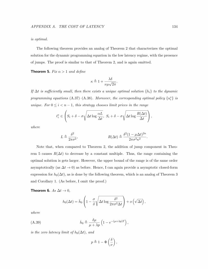
APPENDIX A. THE COST OF LATENCY 134
is optimal.
The following theorem provides an analog of Theorem 2 that characterizes the optimal
solution for the dynamic programming equation in the low latency regime, with the presence
of jumps. The proof is similar to that of Theorem 2, and is again omitted.
Theorem 5. Fix α > 1 and define
κ , 1 + λδ
νµ√
2π.
If ∆t is sufficiently small, then there exists a unique optimal solution hi to the dynamic
programming equations (A.37)–(A.38). Moreover, the corresponding optimal policy u∗i is
unique. For 0 ≤ i < n− 1, this strategy chooses limit prices in the range
`∗i ∈
Si + δ − σ
√∆t log αL∆t , Si + δ − σ
√∆t log R(∆t)
∆t
,where
L ,δ2
2πσ2 , R(∆t) , δ2(1− µ∆t)2n
2πσ2κ2 .
Note that, when compared to Theorem 2, the addition of jump component in Theo-
rem 5 causes R(∆t) to decrease by a constant multiple. Thus, the range containing the
optimal solution is gets larger. However, the upper bound of the range is of the same order
asymptotically (as ∆t→ 0) as before. Hence, I can again provide a asymptotic closed-form
expression for h0(∆t), as is done by the following theorem, which is an analog of Theorem 3
and Corollary 1. (As before, I omit the proof.)
Theorem 6. As ∆t→ 0,
h0(∆t) = h0
1− σ
δ
√∆t log δ2
2πσ2∆t
+ o(√
∆t),
where
(A.39) h0 ,δµ
µ+ λp
(1− e−(µ+λp)T
),
is the zero latency limit of h0(∆t), and
p , 1− Φ(δ
ν
),
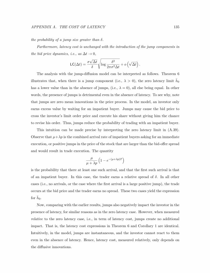
APPENDIX A. THE COST OF LATENCY 135
the probability of a jump size greater than δ.
Furthermore, latency cost is unchanged with the introduction of the jump components in
the bid price dynamics, i.e., as ∆t→ 0,
LC(∆t) = σ√
∆tδ
√log δ2
2πσ2∆t + o(√
∆t).
The analysis with the jump-diffusion model can be interpreted as follows. Theorem 6
illustrates that, when there is a jump component (i.e., λ > 0), the zero latency limit h0
has a lower value than in the absence of jumps, (i.e., λ = 0), all else being equal. In other
words, the presence of jumps is detrimental even in the absence of latency. To see why, note
that jumps are zero mean innovations in the price process. In the model, an investor only
earns excess value by waiting for an impatient buyer. Jumps may cause the bid price to
cross the investor’s limit order price and execute his share without giving him the chance
to revise his order. Thus, jumps reduce the probability of trading with an impatient buyer.
This intuition can be made precise by interpreting the zero latency limit in (A.39).
Observe that µ+λp is the combined arrival rate of impatient buyers asking for an immediate
execution, or positive jumps in the price of the stock that are larger than the bid-offer spread
and would result in trade execution. The quantity
µ
µ+ λp
(1− e−(µ+λp)T
)is the probability that there at least one such arrival, and that the first such arrival is that
of an impatient buyer. In this case, the trader earns a relative spread of δ. In all other
cases (i.e., no arrivals, or the case where the first arrival is a large positive jump), the trade
occurs at the bid price and the trader earns no spread. These two cases yield the expression
for h0.
Now, comparing with the earlier results, jumps also negatively impact the investor in the
presence of latency, for similar reasons as in the zero latency case. However, when measured
relative to the zero latency case, i.e., in term of latency cost, jumps create no additional
impact. That is, the latency cost expressions in Theorem 6 and Corollary 1 are identical.
Intuitively, in the model, jumps are instantaneous, and the investor cannot react to them
even in the absence of latency. Hence, latency cost, measured relatively, only depends on
the diffusive innovations.
APPENDIX A. THE COST OF LATENCY 136
Note that I have thus far assumed Gaussian jump sizes. In Theorem 6, the only place
that this distribution or its parameter ν arises explicitly is the quantity p. This is the
probability that the jump will be larger than the prevailing bid-offer spread, δ, and hence
will cross with the limit order places by the investor. This leads us to conjecture (without
proof) the result in the non-Gaussian case: if the jump size Yi in (A.35) is an i.i.d. zero
mean random variable that has a cumulative distribution function G, then Theorem 6 holds
with p , 1−G(δ).
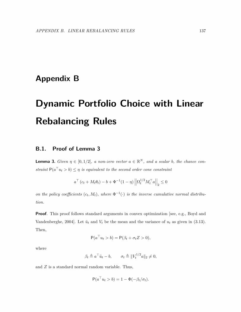
APPENDIX B. LINEAR REBALANCING RULES 137
Appendix B
Dynamic Portfolio Choice with Linear
Rebalancing Rules
B.1. Proof of Lemma 3
Lemma 3. Given η ∈ [0, 1/2], a non-zero vector a ∈ RN , and a scalar b, the chance con-
straint P(a>ut > b) ≤ η is equivalent to the second order cone constraint
a> (ct +Mtθt)− b+ Φ−1(1− η)∣∣∣∣∣∣Ω1/2
t M>t a∣∣∣∣∣∣
2≤ 0
on the policy coefficients (ct,Mt), where Φ−1(·) is the inverse cumulative normal distribu-
tion.
Proof. This proof follows standard arguments in convex optimization [see, e.g., Boyd and
Vandenberghe, 2004]. Let ut and Vt be the mean and the variance of ut as given in (3.13).
Then,
P(a>ut > b) = P(βt + σtZ > 0),
where
βt , a>ut − b, σt , ‖V 1/2
t a‖2 6= 0,
and Z is a standard normal random variable. Thus,
P(a>ut > b) = 1− Φ(−βt/σt).
APPENDIX B. LINEAR REBALANCING RULES 138
Note that the this probability is less than or equal to η if and only if
βt + Φ−1(1− η)σt ≤ 0.
Substituting (3.13) into definitions for βt and σt, we obtain the desired result.
B.2. Exact Formulation of the Terminal Wealth Objective
Following the notation of Section 3.4, I will compute E[W (x, r)2] analytically and demon-
strate that the resulting expression is a quadratic convex function of the policy coefficients.
Without loss of generality, assume that W0 = 0 and µt = 0. Then, observe that
E[W (x, r)2
]=
T∑t=1
T∑k=1
E[(x>t rt+1)(x>k rk+1)
]
=T∑t=1
E[x>t ε
(2)t+1
(ε(2)t+1
)>xt
]+
T∑t=1
T∑k=1
E[x>t Bftf
>k B
>xk]
=T∑t=1
E[x>t ε
(2)t+1
(ε(2)t+1
)>xt
]+
T∑t=1
E[x>t Bftf
>t B
>xt]
+ 2T∑t=1
t∑k=1
E[x>t Bftf
>k B
>xk].
(B.1)
I will consider each of the three terms in (B.1) separately.
The first term can be evaluated he first expectation, E[x>t ε
(2)t+1
(ε(2)t+1
)>xt
], can be eval-
uated in the following form:
E[x>t ε
(2)t+1
(ε(2)t+1
)>xt
]= E
[x>t E
[ε(2)t+1
(ε(2)t+1
)>|Ft]xt
]= E
[x>t Σxt
]= (dt + Ptθt)>Σ (dt + Ptθt) + tr
(ΣPtΩtP
>t
).
Using the representation for xt, I obtain
E[x>t Bftf
>t B
>xt]
= E
(dt +t∑
s=1Js,tfs
)>Bftf
>t B
>(dt +
t∑s=1
Js,tfs
) ,which can be simplified further to
E(
dt +t−1∑s=1
Js,tfs + Jt,t((I − Φ)ft−1 + ε
(1)t
)>)B((I − Φ)ft−1 + ε
(1)t
) ((I − Φ)ft−1 + ε
(1)t
)>B>
(dt +
t−1∑s=1
Js,tfs + Jt,t((I − Φ)ft−1 + ε
(1)t
)).
APPENDIX B. LINEAR REBALANCING RULES 139
The resulting computation deals with taking expectations of the product of jointly normal
random variables with integer exponents:
E
(dt +t−1∑s=1
Js,tfs + Jt,t(I − Φ)ft−1
)>B(I − Φ)ft−1 (B(I − Φ)ft−1)>
(dt +
t−1∑s=1
Js,tfs + Jt,t(I − Φ)ft−1
)+ E
(dt +t−1∑s=1
Js,tfs + Jt,t(I − Φ)ft−1
)>ε(1)t
(ε(1)t
)>(dt +
t−1∑s=1
Js,tfs + Jt,t(I − Φ)ft−1
)+ E
[(ε(1)t
)>B(I − Φ)ft−1 (B(I − Φ)ft−1)> ε(1)
t
]+ E
[(ε(1)t
)>ε(1)t
(ε(1)t
)>ε(1)t
]First define
ψ2 , E[(ε(1)t
)>ε(1)t
(ε(1)t
)>ε(1)t
]=
K∑i=1
3Ψii + 2K∑i=1
i∑j=1
Ψij ,
where Ψij is the (i, j)th entry of the covariance matrix of the error terms for factor dynamics,
Ψ. Using iterated expectations by conditioning on the information up to t − 1, Ft−1,
E[x>t Bftf
>t B
>xt]
equals
E
(dt +t−1∑s=1
Js,tfs + Jt,t(I − Φ)ft−1
)>B(I − Φ)ft−1 (B(I − Φ)ft−1)>
(dt +
t−1∑s=1
Js,tfs + Jt,t(I − Φ)ft−1
)+(dt + Pt−1θt−1
)>Ψ(dt + Pt−1θt−1
)+tr
(Pt−1Ωt−1P
>t−1
)tr(B(I − Φ)Ωt−1
t (B(I − Φ))>Ψ)+ψ2.
where
(B.2) Pt−i ,[J1,t J2,t . . . Jt−i−1,t Jt−i,t
], Jt−i,t ,
(i∑
k=0Jt−k,t(I − Φ)i−k
).
I continue conditioning in a recursive fashion, and finally obtain the deterministic form
E[x>t Bftf
>t B
>xt]
=(dt +
t∑s=1
Js,t(I − Φ)sf0
)>B(I − Φ)tf0
(B(I − Φ)tf0
)>(dt +
t∑s=1
Js,t(I − Φ)sf0
)
+t∑i=1
((dt + Pt−iθt−i
)>Ψ(dt + Pt−iθt−i
)+ tr
(Pt−iΩt−iP
>t−i
)tr(B(I − Φ)iΩt−i
t
(B(I − Φ)i
)>Ψ)
+ ψ2),
which is convex quadratic function of the linear policy parameters.
The third expectation, E[x>t Bftf
>k B
>xk], can be computed using the same procedure.
APPENDIX B. LINEAR REBALANCING RULES 140
B.3. Derivation of the LQC Policies
I can derive a closed form solution for the trading policy when the problem satisfies the LQC
framework. I guess a functional form for the value function and show that this functional
form is preserved at each time step.
Using dynamic programming principle and ut = (xt−xt−1), the value function Vt(xt−1, ft)
satisfies
Vt−1(xt−1, ft) = maximizext
(x>t (Bft)−
12(xt − xt−1)>Λ(xt − xt−1) + E[Vt(xt, ft+1)]
).
I guess the following quadratic form for the value function:
Vt(xt, ft+1) = −12x>t Axx,txt + x>t Axf,tft+1 + 1
2f>t+1Aff,tft+1 + 1
2mt.
Then,
E[Vt(xt, ft+1)] = −12x>t Axx,txt+x>t Axf,t (I − Φ) ft+
12f>t (I − Φ)>Aff,t (I − Φ) ft+
12 (tr(ΨAff,t) +mt) .
At the the last period, I need xT = 0, and the value function equals
VT−1(xT−1, ft) = −12x>T−1ΛxT−1
which satisfies the functional form with
Axx,T−1 = Λ Axf,T−1 = 0 Aff,T−1 = 0 mT−1 = 0.
For all t < T − 1, I maximize the quadratic objective −12x>t Qtxt + x>t qt + bt where
Qt = Λ +Axx,t
qt = Λxt−1 + (B +Axf,t (I − Φ)) ft
bt = −12x>t−1Λxt−1 + 1
2f>t (I − Φ)>Aff,t (I − Φ) ft + tr(ΨAff,t) +mt
Then, the optimal xt is given by Q−1t qt and xt and ut are given by
xt = (Λ +Axx,t)−1 (Λxt−1 + (B +Axf,t (I − Φ)) ft)
ut = (Λ +Axx,t)−1 (Λxt−1 + (B +Axf,t (I − Φ)) ft)− xt−1
APPENDIX B. LINEAR REBALANCING RULES 141
The maximum then occurs at 12q>t Q−1t qt + bt and I obtain the following recursions:
Axx,t−1 = −Λ (Λ +Axx,t)−1 Λ + Λ
Axf,t−1 = Λ (Λ +Axx,t)−1 (B +Axf,t (I − Φ))
Aff,t−1 = (B +Axf,t (I − Φ))> (Λ +Axx,t)−1 (B +Axf,t (I − Φ)) + (I − Φ)>Aff,t (I − Φ)
mt−1 = tr(ΨAff,t) +mt
Using these recursions, I can compute the optimal expected payoff of the dynamic pro-
gram. Using f0 = N(0,Ω0),
E[V0(x0, f1)] = E [E[V0(x0, f1)|f0]]
= E[−1
2x>0 Axx,0x0 + x>0 Axf,0 (I − Φ) f0 + 1
2f>0 (I − Φ)>Aff,0 (I − Φ) f0 + 1
2 (tr(Ω0Aff,0) +m0)]
= −12x>0 Axx,0x0 + 1
2
(tr(Ω0(I − Φ)>Aff,0(I − Φ)
)+T−2∑t=0
tr(ΨAff,0)).
B.4. Exact Formulation of Best Linear Execution Policy
I will first compute the expectation in the objective of (3.29) and write the equivalent de-
terministic form. I will then replace probabilistic constraints with deterministic constraints
using Lemma 3, and finally obtain the deterministic version of the stochastic program in
(3.29)
I start working with the expectation in the objective function. For each t, I have to
compute the expectation of the following two terms, E[x>t (Bft)
], and E
[u>t Λut
]. First, I
derive the statistics for ft, ut and xt. I first note that
ft = (I − Φ)tf0 +t∑
s=1(I − Φ)t−sε(1)
s .
Letting Ft , (f1, . . . , ft)>, Then, in vector form, I have the following representation
Ft =
(I − Φ)f0
(I − Φ)2f0...
(I − Φ)t−1f0
(I − Φ)tf0
+
I 0 . . . 0 0
(I − Φ) I 0 . . . 0... (I − Φ) . . . . . . 0
(I − Φ)t−1 . . .. . . I 0
(I − Φ)t . . . (I − Φ) I
︸ ︷︷ ︸
,At
ε(1)1
ε(1)2...
ε(1)t−1
ε(1)t
.
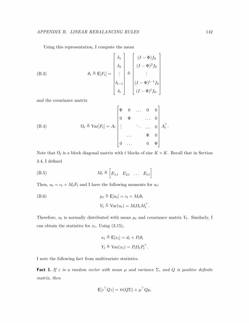
APPENDIX B. LINEAR REBALANCING RULES 142
Using this representation, I compute the mean
(B.3) θt , E[Ft] =
δ1
δ2...
δt−1
δt
,
(I − Φ)f0
(I − Φ)2f0...
(I − Φ)t−1f0
(I − Φ)tf0,
and the covariance matrix
(B.4) Ωt , Var[Ft] = At
Ψ 0 . . . 0 0
0 Ψ . . . 0... . . . . . . 0
. . . Ψ 0
0 . . . 0 Ψ
A>t .
Note that Ωt is a block diagonal matrix with t blocks of size K ×K. Recall that in Section
3.4, I defined
(B.5) Mt ,[E1,t E2,t . . . Et,t
]Then, ut = ct +MtFt and I have the following moments for ut:
µt , E[ut] = ct +Mtθt(B.6)
Vt , Var(ut) = MtΩtM>t .
Therefore, ut is normally distributed with mean µt and covariance matrix Vt. Similarly, I
can obtain the statistics for xt. Using (3.15),
κt , E[xt] = dt + Ptθt
Yt , Var(xt) = PtΩtP>t .
I note the following fact from multivariate statistics.
Fact 1. If z is a random vector with mean µ and variance Σ, and Q is positive definite
matrix, then
E[z>Qz] = tr(QΣ) + µ>Qµ.
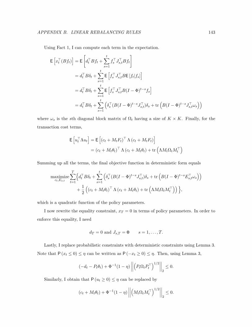
APPENDIX B. LINEAR REBALANCING RULES 143
Using Fact 1, I can compute each term in the expectation.
E[x>t (Bft)
]= E
[d>t Bft +
t∑s=1
f>s J>s,tBft
]
= d>t Bδt +t∑
s=1E[f>s J
>s,tBE [ft|fs]
]
= d>t Bδt +t∑
s=1E[f>s J
>s,tB(I − Φ)t−sfs
]
= d>t Bδt +t∑
s=1
(δ>s (B(I − Φ)t−sJ>s,t)δs + tr
(B(I − Φ)t−sJ>s,tωs
))where ωs is the sth diagonal block matrix of Ωt having a size of K × K. Finally, for the
transaction cost terms,
E[u>t Λut
]= E
[(ct +MtFt)> Λ (ct +MtFt)
]= (ct +Mtθt)> Λ (ct +Mtθt) + tr
(ΛMtΩtM
>t
)Summing up all the terms, the final objective function in deterministic form equals
maximizect,Es,t
T∑t=1
d>t Bδt +
t∑s=1
(δ>s (B(I − Φ)t−sJ>s,t)δs + tr
(B(I − Φ)t−sE>s,tωs
))+ 1
2((ct +Mtθt)> Λ (ct +Mtθt) + tr
(ΛMtΩtM
>t
)),
which is a quadratic function of the policy parameters.
I now rewrite the equality constraint, xT = 0 in terms of policy parameters. In order to
enforce this equality, I need
dT = 0 and Js,T = 0 s = 1, . . . , T.
Lastly, I replace probabilistic constraints with deterministic constraints using Lemma 3.
Note that P (xt ≤ 0) ≤ η can be written as P (−xt ≥ 0) ≤ η. Then, using Lemma 3,
(−dt − Ptθt) + Φ−1(1− η)∣∣∣∣∣∣∣∣(PtΩtP
>t
)1/2∣∣∣∣∣∣∣∣
2≤ 0.
Similarly, I obtain that P (ut ≥ 0) ≤ η can be replaced by
(ct +Mtθt) + Φ−1(1− η)∣∣∣∣∣∣∣∣(MtΩtM
>t
)1/2∣∣∣∣∣∣∣∣
2≤ 0.
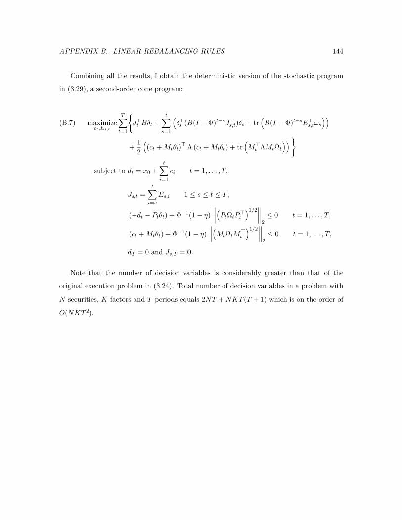
APPENDIX B. LINEAR REBALANCING RULES 144
Combining all the results, I obtain the deterministic version of the stochastic program
in (3.29), a second-order cone program:
maximizect,Es,t
T∑t=1
d>t Bδt +
t∑s=1
(δ>s (B(I − Φ)t−sJ>s,t)δs + tr
(B(I − Φ)t−sE>s,tωs
))(B.7)
+ 12((ct +Mtθt)> Λ (ct +Mtθt) + tr
(M>t ΛMtΩt
))
subject to dt = x0 +t∑i=1
ci t = 1, . . . , T,
Js,t =t∑i=s
Es,i 1 ≤ s ≤ t ≤ T,
(−dt − Ptθt) + Φ−1(1− η)∣∣∣∣∣∣∣∣(PtΩtP
>t
)1/2∣∣∣∣∣∣∣∣
2≤ 0 t = 1, . . . , T,
(ct +Mtθt) + Φ−1(1− η)∣∣∣∣∣∣∣∣(MtΩtM
>t
)1/2∣∣∣∣∣∣∣∣
2≤ 0 t = 1, . . . , T,
dT = 0 and Js,T = 0.
Note that the number of decision variables is considerably greater than that of the
original execution problem in (3.24). Total number of decision variables in a problem with
N securities, K factors and T periods equals 2NT +NKT (T + 1) which is on the order of
O(NKT 2).