
Dynamic Substructuring of an A600 Wind Turbine - DiVA …735329/FULLTEXT01.pdf · Dynamic...
41
Master Thesis in Mechanical Engineering Dynamic Substructuring of an A600 Wind Turbine Author: Ahmed Alkaysee & Marek Wronski Surpervisor LNU: Andreas Linderholt Examinar, LNU: Andreas Linderholt Course Code: 4MT01E Semester: Spring 2014, 15 credits Linnaeus University, Faculty of Technology
Transcript of Dynamic Substructuring of an A600 Wind Turbine - DiVA …735329/FULLTEXT01.pdf · Dynamic...

Master Thesis in Mechanical Engineering
Dynamic Substructuring
of an A600 Wind Turbine
Author: Ahmed Alkaysee & Marek Wronski
Surpervisor LNU: Andreas Linderholt
Examinar, LNU: Andreas Linderholt
Course Code: 4MT01E
Semester: Spring 2014, 15 credits
Linnaeus University, Faculty of Technology


III
Abstract
A limited and extendable master thesis is representing the first step in the
experimental substructuring of an A600 wind turbine. Additional masses have been
designed, manufactured and added to the sub components for the laboratory
experimental tests. Further preparations for dynamic experimental tests have been
described and implemented. Vibrational tests of a modified wind turbine blade have
been made using the Leuven Measurements System (LMS) for excitations and data
acquisition purposes. The theory of frequency response function based substructuring
applied on the wind turbine blade model is demonstrated. The theory and an example
of a Matlab coded spring-mass system, an experimental model of a wind turbine
blade and FRFs stemming from measurements are reported.
Key words: Substructural techniques, wind turbine, blade, decoupled, FRF, dynamic
substructuring.

IV
Acknowledgement
We highly appreciate the help we have got to succeed in our master thesis proposal,
and we sincerely would like to direct many thanks to:
- Mr. Andreas Linderholt, (Linnaeus University, Department of Mechanical
Engineering, Vaxjo) for his comprehensive attention, sophisticated support
and supervision of the project.
- Mr. Leif Petersson, (Linnaeus University, Department of Mechanical
Engineering, Vaxjo) for his help in preparing the additional components used
for the measurements structure.

V
Table of contents
1. INTRODUCTION...................................................................................................... 1
1.1 BACKGROUND ....................................................................................................................................... 1 1.2 PURPOSE AND AIM ................................................................................................................................ 1 1.3 HYPOTHESIS AND LIMITATIONS ............................................................................................................. 2 1.4 RELIABILITY, VALIDITY AND OBJECTIVITY ............................................................................................ 3
2. THEORY .................................................................................................................... 4
2.1 INTRODUCTION TO THE SUBSTRUCTURING ANALYSES ........................................................................... 4 2.2 COUPLING IN THE PHYSICAL DOMAIN .................................................................................................... 5 2.3 THEORETICAL PART MODEL ................................................................................................................... 6 2.4 BEAM MODEL...................................................................................................................................... 11 2.5 VIBRATIONAL ANALYSES .................................................................................................................... 14
3. METHOD ................................................................................................................. 16
3.1 METHODOLOGY STEPS ......................................................................................................................... 16 3.2 VIBRATIONAL TEST ............................................................................................................................. 17
4. RESULTS ................................................................................................................. 25
5. ANALYSIS ............................................................................................................... 27
5.1 THEORETICAL MODEL (SPRING-MASS SYSTEM) .................................................................................... 27 5.2 EXPERIMENTAL MODEL (TURBINE BLADE)........................................................................................... 28
6. DISCUSSION ........................................................................................................... 29
7. CONCLUSIONS ...................................................................................................... 30
REFERENCES ................................................................................................................. 31
APPENDIX 1: THE PROJECT TIME SCHEDULE ..................................................... 1
APPENDIX 2 ...................................................................................................................... 1

1
Ahmed Alkaysee& Marek Wronski
1. Introduction
An interesting point of view in engineering is to divide a structure into
smaller parts in order to simplify the test and the analysis and correlation,
and to compare between different systems as well. In numerical techniques
this concept is considered as the basis of Finite Element discretization.
Recently, it has been a renewed interest in using measurements to make a
dynamic model for some parts and assembling them with numerical models
to predict the behavior of the complete structure. One advantage of checking
a complex system in components is that the model can be validated more
easily and problems can be detected more exactly.
Substructured models are comprehensive; when one part is modified then it
can be readily assembled with the other intact components to predict the
global behavior. Experimental substructuring has become applicable to
difficult engineering problems. Much success has come as a consequence
due of advancement in measurement hardware and software, and new
methods which overcome the problem of incomplete information and
measurement errors.
The dynamic substructuring has a great value in performing the analyses of a
structural system and some important advantages over global methods where
the entire problem is handled by allowing:
- Evaluation the dynamic behavior of the large structures which are
difficult to be tested as a whole.
- Sharing and assembling of the substructures from different groups.
1.1 Background
The SEM (Society of Experimental Mechanics) Focus Group has chosen
theAmpair600W wind turbine as a benchmark test model for substructuring
studies. This master thesis work concerns substructuring studies of the
Ampair 600W wind turbine.
1.2 Purpose and Aim
The experimental substructuring techniques in use today work on simple
academic examples but their use on the real world problems have been
restrained by poor results due to a lot of degrees of freedom systems.
The purpose of this thesis work is to study substructuring techniques using
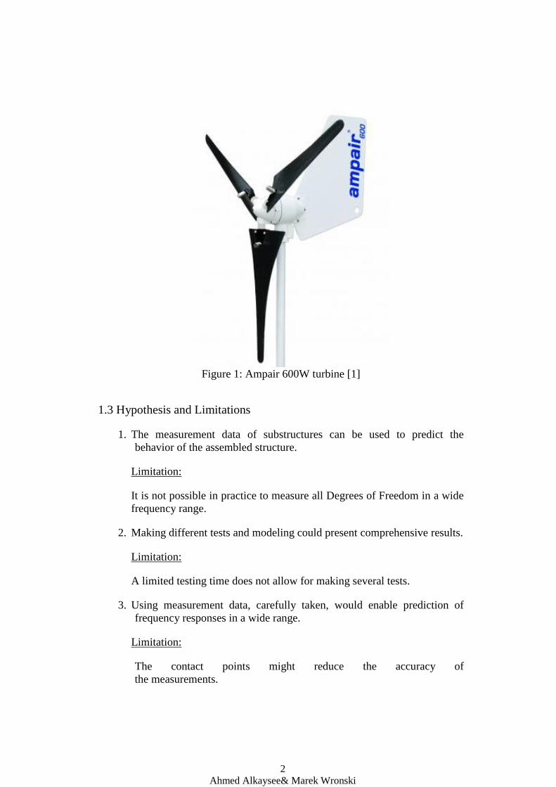
parts of the Ampair 600W wind turbine, shown in Figure 1 as the test
structure. The aim of the work is to increase the knowledge of the chosen
substructuring method and preparing the structure for further testing.
2
Ahmed Alkaysee& Marek Wronski
Figure 1: Ampair 600W turbine [1]
1.3 Hypothesis and Limitations
1. The measurement data of substructures can be used to predict the
behavior of the assembled structure.
Limitation:
It is not possible in practice to measure all Degrees of Freedom in a wide
frequency range.
2. Making different tests and modeling could present comprehensive results.
Limitation:
A limited testing time does not allow for making several tests.
3. Using measurement data, carefully taken, would enable prediction of
frequency responses in a wide range.
Limitation:
The contact points might reduce the accuracy of
the measurements.
3
Ahmed Alkaysee& Marek Wronski
1.4 Reliability, validity and objectivity
The benefits of dynamic substructuring have not yet become a common tool
for the structural dynamic engineers. Therefore, the objective of the work
presented in this thesis can be formulated as:
“Develop a practical modeling framework based on the concept of dynamic
substructuring that enables detailed, integrated structural dynamic analysis
of the wind turbines without compromising on computational efficiency.”[2]
The main objective of thesis can be divided into two sub problems:
1. Develop the dynamic substructuring methodology in a synthetic way
using a Matlab code.
2. Make experimental vibrational tests on different subparts of the
structure.
The majority of the dynamic analyses of the wind turbine are presented by
simulating and modeling. The major commitment of this thesis focuses on
the methodology of vibrational tests of the assembled and dismantled
structures. In order to validate the measurements´ results, several tests are
conducted on a specific model of connection between the turbine hub and
blades which will be described in the Method chapter.

4
Ahmed Alkaysee& Marek Wronski
2. Theory
2.1 Introduction to the substructuring analyses
Figure 2 shows an example of substructuring as mentioned previously, that
is an operation where separate components of a structure are tested and
analyzed individually.
Figure 2: Car example for substructuring [3]
Analytical substructuring is based on the Finite Element Methods and linked
with some technique methods such as the Craig-Bampton method. This
method reduces the size of a finite element model, while the experimental
substructuring is less common in practice.
Here are some general concepts in substructuring:
Substructuring;
Reduction of dynamic models;
Assembly of substructures;
Degrees of freedom reduction;
Experimental substructuring.

5
Ahmed Alkaysee& Marek Wronski
2.2 Coupling in the physical domain
Nomenclature:
FRF= frequency response function
DOF= degrees of freedom
LMS= Leuven Measurements System
B = signed Boolean matrix
C = damping matrix
f = vector of external forces
g = vector of connecting forces
K = stiffness matrix
L = Boolean localization matrix
M = mass matrix
q = vector of unique degrees of freedom
u = vector of degrees of freedom
= vector of Lagrange multipliers
The system described by its mass, damping and stiffness matrices as
determined from the mechanical and geometrical properties is called the
physical domain [8], and the equation of motion in this domain of a discrete
dynamic subsystem can be expressed as:
( ) ( ) ( ) ( ) ( ) (1)
Here, is the external force vector, and is the vector of the connecting
forces with other substructures. The connecting forces can be considered as
constraining forces associated with compatibility conditions, it is here
assumed that the system is linear and time invariant.

6
Ahmed Alkaysee& Marek Wronski
2.3 Theoretical part (3 dof spring-mass system)
The Figure 3 shows another example for another 3 dof spring-mass model
which is considered as the theoretical part of this work and will be coded by
Matlab program and analyzed.
Figure 3: Assembled spring-mass system
The equations of motion for the assembled 3 degrees of freedom system are
represented by the matrices
[
] {
} [
] {
} {
} (2)
Coupling the physical model and the assembled 3 degree of freedom system
shown inFigure 3is described by the following equations:
The local equilibrium equation:
(6) (3)
[
] [
] [
](4)

7
Ahmed Alkaysee& Marek Wronski
The equilibrium equation for the connecting forces:
[
] [
]
(5)
The interface compatibility equation:
[ ] [
]
(6)
By dismantling the spring-mass system into two parts, Figure 5 shows the
left hand side part of substructure A with the applied force and only 2 dof.
Substructure A
Figure 4: Substructure A, left hand side
The equation of motion for this part is represented by the matrices
[
] { } [
] { } {
} (7)
8
Ahmed Alkaysee& Marek Wronski
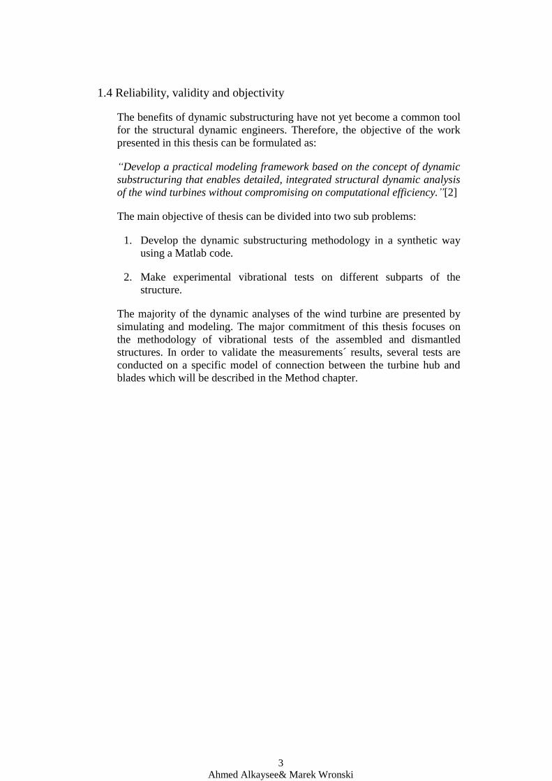
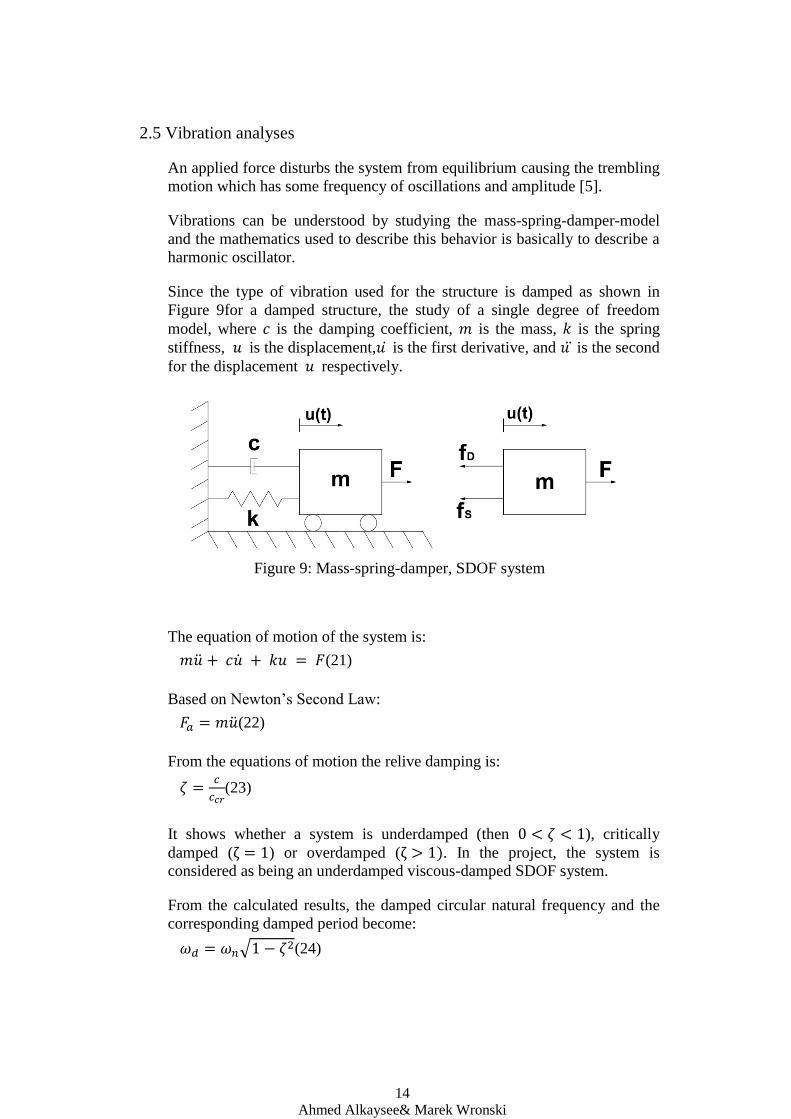
The right hand side of the structure is shown here in Figure 5, with 2 dof as
well.
Substructure B
Figure 5: Substructure B, right hand side
And the equations of motion for this part is
[
] { } [
] { } {
} (8)

9
Ahmed Alkaysee& Marek Wronski
The next two graphs in Figure 6show the frequency response of the two
substructures A and B which were illustrated in Figure 5 and Figure 6
respectively, as a reaction to the applied excitation. They represent the
theoretical FRF results calculated using Matlab code.
Figure 6: Matlab code FRF, 2dof spring- mass substructures

10
Ahmed Alkaysee& Marek Wronski
Figure 7: Matlab code FRF, 3 dof spring-mass assembly
An assembly case shows coherent results like an adding response function
structure A to B when they be combined together in one structure, which
means that the theoretical modeling corresponds with the aim of
substructuring. The codes [9] for the frequency response function in this
example are explained in appendix A2.

11
Ahmed Alkaysee& Marek Wronski
2.4 Beam Model
For another kind of mechanical systems, a beam model can be considered,
and coupling the substructures of this model builds up to12 DOF system as
shown in Figure 8, and described by the following equations
(9)
(10)
( ) (11)
(12)
( ) ( ) ( ) (13)
The equation will be naturally satisfied since the primal degrees of
freedom sum to zero.
Figure 8: Beam substructure model, 12 dof

12
Ahmed Alkaysee& Marek Wronski
Primal assembly: Coupling the physical model initially by considering the
compatible set of the degrees-of-freedom
[ ]
[ ]
[ ]
(14)
Dual assembly: Coupling the physical model also by the same consideration
to the compatible set of DOF using the equations
(15)
(16)
(17)
(21)
[
] [ ] [
] [ ]+[
] [ ] [
] (18)
Therefore, the equation will be naturally satisfied as well since the
connection forces on dual degrees of freedom sum to zero.

13
Ahmed Alkaysee& Marek Wronski
[ ]
[ ]
(19)
[ ]
[ ]
; ; ;
(20)
14
Ahmed Alkaysee& Marek Wronski
2.5 Vibration analyses
An applied force disturbs the system from equilibrium causing the trembling
motion which has some frequency of oscillations and amplitude [5].
Vibrations can be understood by studying the mass-spring-damper-model
and the mathematics used to describe this behavior is basically to describe a
harmonic oscillator.
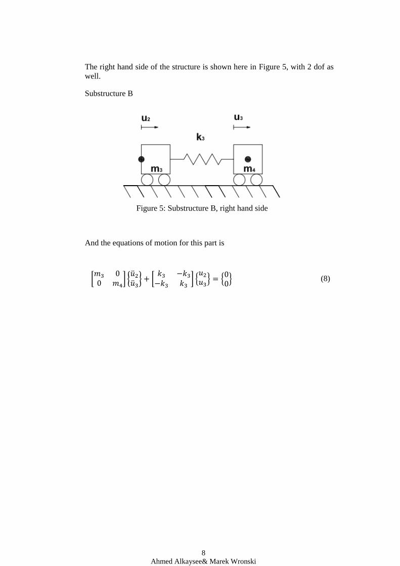
Since the type of vibration used for the structure is damped as shown in
Figure 9for a damped structure, the study of a single degree of freedom
model, where is the damping coefficient, is the mass, is the spring
stiffness, is the displacement, is the first derivative, and is the second
for the displacement respectively.
Figure 9: Mass-spring-damper, SDOF system
The equation of motion of the system is:
(21)
Based on Newton’s Second Law:
(22)
From the equations of motion the relive damping is:
(23)
It shows whether a system is underdamped (then ), critically
damped ( ) or overdamped ( ). In the project, the system is
considered as being an underdamped viscous-damped SDOF system.
From the calculated results, the damped circular natural frequency and the
corresponding damped period become:
√ (24)

15
Ahmed Alkaysee& Marek Wronski
(25)
The general solution for an SDOF system can be written using the Euler
formula as:
( ) ( ) (26)
Real structures contain an infinite number of DOF and many natural
frequencies as well. Not all the frequencies are needed since they will not be
excited or they have very low amplitudes [5].
The vibrational analyses can be made either in the time domain or in the
frequency domain, and this is related by the Fourier transformation:
( ) ∫ ( ) ( )
(27)
This can be treated as a special case of Laplace transformation. Time
domain response shows how the system behaves when exposed to a certain
excitation in a domain of time. Frequency domain shows how the material
behaves when it is exposed to a certain frequency spectrum.
The frequency response equation is:
( ) ( ) ( ) ( )
( ) (28)
Here, ( ) is the frequency response function, and ( )is the Fourier
transform of the excitation.
According to the mathematical model ( ) and ( ) vary depending on the
type of problem. For a viscously-damped SDOF, the frequency response is
given by:
( )
⁄
[ ( ⁄ )
] ( ⁄ )
(29)

16
Ahmed Alkaysee& Marek Wronski
3. Method
3.1 Methodology steps
The substructuring work will be followed until the satisfactory approach
with respect to:
1. Component modeling: Dismantling the system into separated parts,
which can be modeled later using the Finite Element Methods, and
the outcomes can be exported to Matlab program.
2. Model validation: The components’ models are validated in order to
evaluate the work accuracy.
3. Degree of freedom reduction: The preliminary models have a large
number of DOF if the finite element is considered, and a necessity
of using reduction techniques is there in order to reach the optimal
representation using the minimum allowable number.
4. Estimation: The dynamic response of each individual component
will be estimated separately, and another estimation for the system
as all before combination.
5. Assembly: The dynamic model of the whole system is approached
by assembling the separated parts all together.
6. Further reduction: By the interface reduction for the degrees-of-
freedom.
7. Model analysis: The analyses are done for both theoretical and
experimental models, and the limited work time led to choose a
spring- mass system for the theoretical part.
8. Validation: Validating the measurements is required for the whole
system after combining all its components together in order to
ensure that the assembled model resembles the right structure.
9. Work updating: Evaluating the analyses of the total model whether
the design is satisfactory. If an additional design change is needed or
another component is reduced or added, then it will be followed by
an update for that change.
17
Ahmed Alkaysee& Marek Wronski
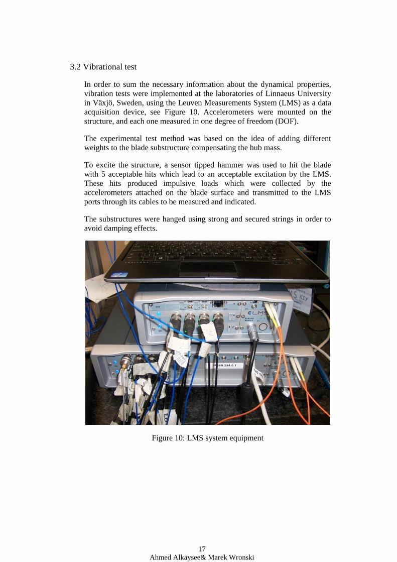
3.2 Vibrational test
In order to sum the necessary information about the dynamical properties,
vibration tests were implemented at the laboratories of Linnaeus University
in Växjö, Sweden, using the Leuven Measurements System (LMS) as a data
acquisition device, see Figure 10. Accelerometers were mounted on the
structure, and each one measured in one degree of freedom (DOF).
The experimental test method was based on the idea of adding different
weights to the blade substructure compensating the hub mass.
To excite the structure, a sensor tipped hammer was used to hit the blade
with 5 acceptable hits which lead to an acceptable excitation by the LMS.
These hits produced impulsive loads which were collected by the
accelerometers attached on the blade surface and transmitted to the LMS
ports through its cables to be measured and indicated.
The substructures were hanged using strong and secured strings in order to
avoid damping effects.
Figure 10: LMS system equipment

18
Ahmed Alkaysee& Marek Wronski
The experimental tests were divided into three parts of different
substructures in order to measure their frequency response, and these parts
are:
Part 1: Turbine blade, holder, cube, bolt-nut joint and mass, Figure 11.
Part 2: Mass, cube and bolt nuts joint, Figure 12.
Part 3: Turbine blade and its holder, Figure 13.
The laboratory test was implemented on each of these 3 substructures
illustrated next in these figures using 3 different masses in part 1 and part 2
and explained in more detail as follows:
1. The first part was done on 3 substructures. Each one of them was
consisting of the components mentioned previously in part 1for each of
the 3 masses of weights: 1kg, 2kg and 4kg respectively as illustrated
next in Figure 11.
A metal cube was put in between the blade and the mounted disc mass in
order to use its 4 round surfaces in the (Z-Y) plane as places to mount
the accelerometers which would measure the degrees-of-freedom in the
(Z) and (Y) directions.
Each mass was mounted together with the turbine blade on the blade
holder side and fastened by a screw- nut joint which comes throughout
the holder.
These accelerometers´ distributions are illustrated in Figure 14 and
explained as follows:
20 accelerometers on the front side of the turbine blade in the (X-Y)
plane, perpendicular to the (-Z) direction.
4 accelerometers on the upper surface of the disc mass around its
center in 90 degrees between each other in the (Z-Y) plane,
perpendicular to the (X) direction.
4 accelerometers on the 4 round surfaces of the cube in the (Z-Y)
plane.
1 accelerometer in the (Z-Y) plane, perpendicular to the cross section
of the connecting screw.

19
Ahmed Alkaysee& Marek Wronski
Figure 11: Assembled structures with 3 added masses
The recorded excitations were made in the 3 directions using the different
sides of the blade, masses and cube components.

20
Ahmed Alkaysee& Marek Wronski
2. The second test included 3different substructures also. Each of them
consisted of the components mentioned previously in part 2 with one of
these 3 masses mounted with a cube by a screw-nut joint and an epoxy
lime as well. Four accelerometers connected to the LMS device were
attached to the upper surface of a mass around its center 90 degrees
between each other, Figure 12.
Figure 12: Substructures of 1kg, 2kg and 4kg masses
The recorded excitations here were made also in the 3 directions using the
different sides for only the masses and cube components.

21
Ahmed Alkaysee& Marek Wronski
3. The third test consisted of only the turbine blade with its holder, see
Figure 13.
Figure 13: Blade and holder substructure
The recorded excitation was made using the same equipment tool in the (-Z)
direction only.

22
Ahmed Alkaysee& Marek Wronski
The accelerometers´ locations on these substructures were given to the LMS
in the geometry nodes input according to the intended places to be attached
on, as illustrated in Figure 14 which shows their distributions on the LMS
screen.
Figure 14: Distributions of the accelerometers on the LMS plot
The LMS equipment tool which was mentioned previously and used to
implement the excitations is the hammer with a sensor tip on the impact
edge and a cable connection on its tail, see Figure 15.
Figure 15: LMS excitation hammer
Force sensor
23
Ahmed Alkaysee& Marek Wronski
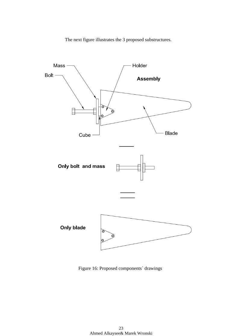
The next figure illustrates the 3 proposed substructures.
Figure 16: Proposed components´ drawings

24
Ahmed Alkaysee& Marek Wronski
More clarification for the different assemblies with respect to the added
masses is presented here in Figure 17.
Figure 17: Assemblies´ models with the added masses

25
Ahmed Alkaysee& Marek Wronski
4. Results
The extracted FRF graphs for the 3substructures with respect to those 3
different masses are shown in Figure18, Figure 19 and
Figure 20 respectively.
Figure 18: Accelerometers´ FRF graphs, 1kg mass substructures
X- axis: Frequency (Hz), (20 - 500)
Y- axis: FRF amplitude (g/N), (0 – 0.1)
Figure 19: Accelerometers´ FRF graphs, 2kg mass substructures
X- axis: Frequency (Hz), (20 - 500)
Y- axis: FRF amplitude (g/N), (0 – 0.1)
26
Ahmed Alkaysee& Marek Wronski
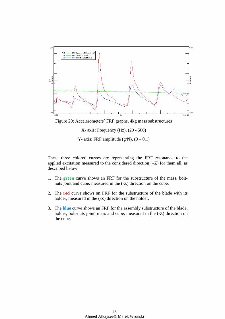
Figure 20: Accelerometers´ FRF graphs, 4kg mass substructures
X- axis: Frequency (Hz), (20 - 500)
Y- axis: FRF amplitude (g/N), (0 – 0.1)
These three colored curves are representing the FRF resonance to the
applied excitation measured to the considered direction (–Z) for them all, as
described below:
1. The green curve shows an FRF for the substructure of the mass, bolt-
nuts joint and cube, measured in the (-Z) direction on the cube.
2. The red curve shows an FRF for the substructure of the blade with its
holder, measured in the (-Z) direction on the holder.
3. The blue curve shows an FRF for the assembly substructure of the blade,
holder, bolt-nuts joint, mass and cube, measured in the (-Z) direction on
the cube.
27
Ahmed Alkaysee& Marek Wronski
5. Analysis
5.1 Theoretical part (spring-mass system)
The graph shown in Figure7 for substructure A, which has 2 proposed DOF,
indicates its FRF to the excitation caused by the applied force onmass 1.
This graph includes the FRF of mass 1 and sub mass 2, Figure 4. The FRF
curves and
for these two masses are sticking together starting from
the amplitude ⁄ to the first FRF at ⁄ for both masses at
1000Hz frequency, and move together along the frequency scope(0-
2500)Hz, which means that both masses are moving together back and forth.
The second graph in the same figure indicates the FRF resonance for
substructure B, which has 2DOF as well, to the excitation of the transmitted
force P. It includes the FRF of sub mass 2 and mass 3, Figure 5.The FRF
indicating curves and
, for these two masses are separated starting
from the amplitude value around ⁄ but departing each other,
upward for mass 4 and downward for sub mass 3. It means that these masses
are not moving together as mass 4 is moving just like the two masses of
substructure A but with lower FRF value approaching the amplitude 1 m/N
at higher frequency of 1250Hz, while it is 0.001 m/N for sub mass 3 at
875Hz.
These FRF values along the frequency extent are dependent on the variation
of the springs´ stiffness and masses besides the magnitude of the exciting
force. It seems as if the FRF changes according to these variables and keeps
fluctuating along the frequency extent. The 2nd
and 3rd
nodal points here are
the reference for the theoretical resulting response calculated by Matlab
program and shown on the graph, as they exist on the interface surface
between the two substructures and contain the 2nd
and 3rd
degrees-of-
freedom respectively.
The third graph, Figure 7, indicates the FRF resonance for the total assembly
of these two substructures to the force excitation. By 3DOF and an
indicating graph includes the FRF of the masses 1, 2 and 3, as illustrated in
Figure 3. The FRF is indicating a united curve for both structures as an
assembly. It starts from the amplitude value ⁄ and moves upward
to the first FRF of ⁄ at 600Hz, and to the second FRF of ⁄ at
1200Hz, then to the last one of ⁄ at 2400Hz.
It seems that the reacting behavior of the substructures is pent in the
assembly restriction, which means that the idea of analyzing separated
components can expose their behavior more closely and lead therefore to
accurate results and behavior estimations.

28
Ahmed Alkaysee& Marek Wronski
5.2 Experimental part (turbine blade model)
The experimental outcomes are expressed by the LMS resulting graphs for
each excitation, as shown previously in Figure 18, Figure 19 and
Figure 20. They are indicating the FRF for those 3 substructures illustrated
previously in the Figures 12, 13 and 14 of the real photos and their proposed
drawings in Figure17. These figures show the FRF for each substructure
represented by an oscillating curve of a different color indicating the
reaction to the applied excitation.
For 1kg mass, the resulting graphs for the acceptable excitations
implemented on those substructures are showing the only mass FRF values
by the green line, while the red line for only the blade, and the blue one for
the total blade-mass assembly, Figure 18.Starting with the upper green line
which is showing the mass resonance to the excitation applied by the
hammer in the (-Z) direction. The FRF line is dropping down from (0.095-
0.078) ⁄ in the beginning with small oscillations along a frequency range
up to 50Hz, then it begins to increase steadily along the rest of the total
frequency extent of 500Hz without more fluctuations. It shows the low
resonance to the excitations owing to its high density. Secondly, the red line
is showing the blade resonance, which starts from the FRF amplitude of
⁄ fluctuating increasingly at frequency peak values100Hz, 200Hz,
315Hz, 440Hz and 480Hz, which shows high resonance of the blade.
Thirdly, the blue line is showing the resonance of the blade-mass assembly,
starting with ⁄ and fluctuating increasingly at the frequency values
of 30Hz, 100Hz, 315Hz, 440Hz and 480Hz harmonically with the blade
FRF but in less scope, which means that the mass FRF is distinctly
influencing and decreasing the FRF of the total assembly.
For 2kg mass mounted with the blade, the FRF has the same appearance but
with lower FRF values for all substructures not only in the start which is
⁄ but also along the frequency scope (20-500) Hz. For the blade and
blade-mass components the FRF starts at the amplitude ⁄ , Figure 19.
The FRF values here are lower than for the substructures of 1kg mass.
For 4kg mounted mass, the same phenomena appears as the FRF resonance
of this mass has the same appearance with much lower amplitude values of
the FRF to start with, which is only ⁄ and also lower values along
the frequency scope (20-500)HZ. For the blade and blade-mass components
the FRF starts from lower amplitude value of ⁄ , and fluctuating
through lower amplitudes,
Figure 20, and consequently the FRFs here are much lower than for the
substructures of masses 1kg and 2kg.

29
Ahmed Alkaysee& Marek Wronski
6. Discussion
The paper of substructuring concept for this model turbine was concluded
after preparing for the test by designing and manufacturing the components
and the added masses with their accessories, proceeding to the test and
validating its results which were the main steps.
Matlab program and LMS equipment were helpful to extract the plotting
graphs both synthetically and experimentally, which show the realistic
resonance of those components to the outside effects. The excitations were
done in the 3 directions on the first 2 assemblies, but in only (-Z) direction
for the blade alone because it was not prepared for excitations in other
directions. Therefore, the only considered outcome data have been collected
from the recorded excitations in the (-Z) direction.
The outcomes graphs for the 3substructures with respect to those 3 different
masses shows that the FRFs for the total blade assembly is equivalent to the
blade FRF after subtracting the mass FRF. In other words, the FRF for the
two substructures must show equivalence to the assembly FRF, most likely
the results of the Matlab code for the theoretical spring-mass model which is
giving the same indication.
30
Ahmed Alkaysee& Marek Wronski
7. Conclusions
A limited master thesis is presenting substructure technique in practical
applications. The framework is outlined by the synthetic spring-mass and
beam systems including primal and dual assembly and followed by the
results´ analyses, and a model wind turbine is used in the experimental part.
Frequency results of the turbine blade combining it with different weights of
masses are comprehensive. They shift the relationship between the
theoretical model and the experimental one. The data from the synthetic
model show perfect results for the frequency response. They indicate the
restricted behavior of the substructures by the assembly coherence and the
possibility of releasing them to expose their initial and close behavior using
substructuring concept, and consequently, lead to the optimal results
approach and behavior estimations. The experimental outcomes of the
frequency response function have demonstrated along the frequency scope
for different dependent masses. They show the FRF equivalence between the
substructured components and their assembly, as well as, the more mounted
mass the lower FRF outcomes not only for the mass itself but for the total
assembly as well.
Studying frequency response based-substructuring in experimental dynamics
and synthetic techniques can lead to forward step in this open issue. It can be
extended for this model turbine in further researches to include more
components, and the data acquisition can be coded for the same
experimental model in a thorough research.

31
Ahmed Alkaysee& Marek Wronski
References
[1] Ampair Energy Ltd, 2014. Ampair Wind, Hydro and Packaged Power
specialists. Available at: http://www.ampair.com/wind-turbines/ampair-
600 [Accessed 20 02 2014].
[2] Voormeeren S.,2012. Dynamic Substructuring Methodologies for
Integrated Dynamic Analysis of Wind Turbines. PhD-Thesis, Delft
University of Technology.
[3] Rixen D. 2010. Dynamic Substructuring Concepts – Tutorial, Delft
University of Technology.
[4] "Mechanical Vibration and Shock Measurements” Available at:
http://www.bksv.com/Library/Primers.aspx [Accessed 20 02 2014].
[5] Encyclopedia Britannica (2014) Available at:
http://www.britannica.com/EBchecked/topic/627269/vibration.
[6] Craig Jr., R. R.& Kurdila, A. J., 1981. Fundamentals of structural
dynamics. 2nd ed. New Jersey: John Wiley & Sons.
[7] Gibanica M., 2013. Experimental-Analytical Dynamic
Substructuring, Master Thesis, Chalmers University of Technology,
Goteborg.
[8] D. de Klerk, D.J. Rixen, S.N. Voormeeren, 2008. General
Framework for Dynamic Substructuring: History, Review, and
Classification of Techniques, Delft University of Technology.
[9] M. S. Allen, D Rixen, R. L. Mayes, 2014. Short Course on
Experimental Dynamic Substructuring, IMAC, Orlando, Florida.

32
Ahmed Alkaysee& Marek Wronski

Appendix 1: 2
Ahmed Alkaysee& Marek Wronski
APPENDIX 1: The project time schedule
Acitvity Time v13 v14 v15 v16 v17 v18 v19 v20 v21 v22 v23
Thesis work Information gathering X X
FEM-modelling
X X X X Calculations models (Matlab)
X X X X
Vibrational test data
X X X Comparision and conclusion
X X
Write thesis report
X X X X X Preliminary report
X X
Presentation
X

Appendix 2: 1
Ahmed Alkaysee& Marek Wronski
APPENDIX 2
% Input data: m1=2.5; % kg m2=2.5; % kg m3=2.5 ;% kg m4=2.5; % kg k1=25e8; % N/m k2=25e8; k3=(1/2)*m3*(1250*2*pi)^2; beta_fact=2*0.01/(1000*2*pi); % stiffness proportional damping
factor
% Create Mass and Stiffness matrices for A, B and C
% Mass Matrix, Stiffness matrix and Damping matrix for structure
A MA=[m1, 0; 0, m2]; KA=[k1+k2, -k2; -k2, k2]; CA=beta_fact*KA;
% Mass Matrix, Stiffness matrix and Damping matrix for structure
B MB=[m3, 0; 0, m4]; KB=[k3, -k3; -k3, k3]; CB=beta_fact*KB;
% Mass Matrix, Stiffness matrix and Damping matrix for structure
C MC=[m1, 0, 0; 0, m2+m3, 0; 0, 0, m4]; KC=[k1+k2, -k2, 0; -k2, k2+k3, -k3; 0, -k3, k3]; CC=beta_fact*KC;
% Make FRFs to use for substructuring: fv = [25:1:2500]*2*pi; % frequency vector in radians/sec FA=zeros(2,length(fv)); FB=zeros(2,length(fv)); FC=zeros(3,length(fv));
% Makeaccelerance FRFs for k=1:length(fv); FA(:,k)=-fv(k).^2*((-fv(k).^2*MA+1i*fv(k)*CA+KA)\[0; 1]);
% unit force in DOF 2

Appendix 2: 2
Ahmed Alkaysee& Marek Wronski
FB(:,k)=-fv(k).^2*((-fv(k).^2*MB+1i*fv(k)*CB+KB)\[1; 0]);
% unit force in DOF 3 FC(:,k)=-fv(k).^2*((-fv(k).^2*MC+1i*fv(k)*CC+KC)\[0; 0; 1]);
% unit force in DOF 4 of assembly end
% Make copies with more convenient names H12A=FA(1,:); H22A=FA(2,:); H33B=FB(1,:); H43B=FB(2,:); H41C=FC(1,:);
% Plots: figure(1) subplot(2,1,1); semilogy(fv/2/pi,abs(FA)); grid on; xlabel('Frequency (Hz)'); ylabel('FRF m/N'); title('Substructure A'); legend('H_{12}^A','H_{22}^A'); subplot(2,1,2); semilogy(fv/2/pi,abs(FB)); grid on; xlabel('Frequency (Hz)'); ylabel('FRF m/N'); title('Substructure B'); legend('H_{33}^B','H_{43}^B');
%% FBS Frequency Based Substructuring H41FBS=H43B.*((H22A+H33B).^-1).*H12A;
%Solution with added noise eps_n=0.0001;
H43Bn=H43B+eps_n*max(abs(H43B))*(randn(size(fv))+1i*randn(size(fv
)));
H22An=H22A+eps_n*max(abs(H22A))*(randn(size(fv))+1i*randn(size(fv
)));
H33Bn=H33B+eps_n*max(abs(H33B))*(randn(size(fv))+1i*randn(size(fv
)));
H12An=H12A+eps_n*max(abs(H12A))*(randn(size(fv))+1i*randn(size(fv
)));
H41FBSn=H43Bn.*((H22An+H33Bn).^-1).*H12An;
figure(2) semilogy(fv/2/pi,abs(H41C),fv/2/pi,abs(H41FBS),'.--
',fv/2/pi,abs(H41FBSn),'-'); grid on; xlabel('Frequency (Hz)'); ylabel('FRF m/N'); title('Assembly C: Frequency Based Substructuring');
legend('H_{41}^C','H_{41}^C FBS','H_{41}^C FBS Noisy');

Faculty of Technology 351 95 Växjö, Sweden Telephone: +46 772-28 80 00, fax +46 470-832 17 (Växjö)