Dynamic stress intensity factors for homogeneous and ... · Dynamic stress intensity factors for...

International Journal of Solids and Structures 43 (2006) 4830–4866

www.elsevier.com/locate/ijsolstr

Dynamic stress intensity factors for homogeneousand smoothly heterogeneous materials using

the interaction integral method

Seong Hyeok Song, Glaucio H. Paulino *

Department of Civil and Environmental Engineering, University of Illinois at Urbana-Champaign, Newmark Laboratory,

205 North Mathews Avenue, Urbana, IL 61801, USA

Received 7 April 2005; received in revised form 17 June 2005Available online 10 October 2005

Abstract

Dynamic stress intensity factors (DSIFs) are important fracture parameters in understanding and predictingdynamic fracture behavior of a cracked body. To evaluate DSIFs for both homogeneous and non-homogeneous mate-rials, the interaction integral (conservation integral) originally proposed to evaluate SIFs for a static homogeneousmedium is extended to incorporate dynamic effects and material non-homogeneity, and is implemented in conjunctionwith the finite element method (FEM). The technique is implemented and verified using benchmark problems. Then,various homogeneous and non-homogeneous cracked bodies under dynamic loading are employed to investigatedynamic fracture behavior such as the variation of DSIFs for different material property profiles, the relation betweeninitiation time and the domain size (for integral evaluation), and the contribution of each distinct term in the interactionintegral.� 2005 Elsevier Ltd. All rights reserved.

Keywords: Dynamic stress intensity factors (DSIFs); Interaction integral; Non-homogeneous materials; Functionally graded materials(FGMs)

1. Introduction

Static and dynamic fracture behavior of homogeneous and non-homogeneous cracked bodies can beunderstood and predicted, to a certain extent, once stress intensity factors (SIFs) are known. Thus, an

0020-7683/$ - see front matter � 2005 Elsevier Ltd. All rights reserved.doi:10.1016/j.ijsolstr.2005.06.102

* Corresponding author. Tel.: +1 217 333 3817; fax: +1 217 265 8041.E-mail addresses: [email protected] (S.H. Song), [email protected] (G.H. Paulino).

mailto:[email protected]

mailto:[email protected]

S.H. Song, G.H. Paulino / International Journal of Solids and Structures 43 (2006) 4830–4866 4831

accurate evaluation of SIFs is crucial in fracture mechanics for both static and dynamic cases as they can beused to investigate crack initiation and propagation. Several methods have been developed and applied bymany researchers to evaluate DSIFs for various problems, as discussed below.

For homogeneous materials, Chen (1975) examined a centrally cracked rectangular finite strip subjectedto step loading using a Lagrangian finite difference method (FDM). DSIFs were obtained from the relationbetween DSIFs and stress fields in the vicinity of a crack tip. This problem has been considered as a bench-mark problem and explored by many researchers. Aoki et al. (1978) utilized the relationship between dis-placements and DSIFs to obtain mode I or mode III DSIFs. Kishimoto et al. (1980) proposed a modifiedpath-independent J-integral, which involves the inertial effects to determine DSIFs in conjunction with thefinite element method (FEM), and employed a decomposition procedure for mixed-mode problems. Bricks-tad (1983) used an explicit time scheme in a special FEM program to evaluate DSIFs. By means of the rela-tionship between SIFs and crack opening displacement, DSIFs were determined without singular elements.Murti and Valliappan (1986) examined various problems, such as Chen�s problem (1975), using quarter-point elements (QPEs) and the FEM. DSIFs were evaluated from the relation between the first twocoefficients of Williams (1957) solution and the finite element displacement in the vicinity of the crack.The effect of QPE size was assessed qualitatively in their works. Lee and Freund (1990) solved mixed modeproblems of a semi-infinite plate containing an edge crack under an impact loading and determined DSIFsthrough linear superposition of several stress wave propagation solutions. Lin and Ballmann (1993) revis-ited Chen�s problem (1975) using the Lagrangian FDM. They adopted the same technique by Chen (1975)to evaluate DSIFs. Their numerical results are almost identical with those obtained by Chen except for afew time periods when wave fluctuations occurs. They contended that Chen (1975) used too few cells tocapture actual peaks of DSIFs. Dominguez and Gallego (1992) computed DSIFs using time domainboundary element method with singular quarter-point boundary elements. Fedelinski et al. (1994) adoptedthe bJ -integral to obtain DSIFs by means of the dual boundary element method. In the bJ -integral approach,the mode decomposition procedure is employed for mixed mode problems. Belytschko (1995) determinedstatic and dynamic SIFs using the Element Free Galerkin (EFG) method, which is a meshless method basedon moving least square interpolants. The DSIFs were calculated by conservation integrals, which directlyevaluate the individual SIFs for the mixed mode problem in terms of known auxiliary solutions. Sladeket al. (1997, 1999) used the bJ -integral to determine DSIFs in conjunction with the boundary element meth-od (BEM). They proposed the interaction integral for the computation of T-stress (non-singular stress), andthe bJ -integral for the evaluation of DSIFs. Krysl and Belytschko (1999) investigated three-dimensional(3D) stationary and dynamically propagating crack problems. DSIFs were obtained from the interactionintegral in conjunction with the EFG method. Zhang (2002) explored transient dynamic problems usinghypersingular time-domain traction BEM. DSIFs were obtained from relating the crack tip openingdisplacements and SIFs. Tabiei and Wu (2003) investigated fracture behavior including DSIFs and energyrelease rate for a cracked body subjected to dynamic loadings using DYNA3D (Whirley and Engelmann,1993), which is a non-linear explicit finite element code. An element deletion-and-replacement remeshingscheme was employed using the FEM to simulate crack propagation. Enderlein et al. (2003) investigatedfracture behavior for two-dimensional (2D) and 3D cracked bodies under impact loading using FEM. Theyadopted the J-integral, the modified crack closure integral and the displacement correlation technique toevaluate pure mode I DSIFs. Fedelinski (2004) applied the dual BEM in conjunction with the time domain,the integral transform and the dual reciprocity methods for dynamic analysis of cracked media whereDSIFs were computed using the relationship between path independent integral and crack openingdisplacements.

For non-homogeneous materials, Rousseau and Tippur (2001) obtained DSIFs for FGMs both numer-ically and experimentally. The DSIFs prior to crack initiation were determined utilizing asymptotic fields ofWilliams� solution (1957), which is equivalent to the stationary fields. After initiation, the crack tip fields forsteadily growing cracks in FGMs, obtained by Parameswaran and Shukla (1999), were used to obtain

4832 S.H. Song, G.H. Paulino / International Journal of Solids and Structures 43 (2006) 4830–4866

DSIFs. Material gradients were employed in the commercial software ABAQUS (2004) by applying tem-perature, which is a function of material properties, and by letting the coefficient of thermal expansion bezero. As the distance is close to the crack tip, the DSIFs were underestimated because no singular elementswere used. Therefore, regression technique was employed to obtain DSIFs at the crack tip based on thedisplacement correlation technique (DCT). Wu et al. (2002) extended the J-integral to incorporate materialgradients and dynamic effects. They evaluated J for a single edge cracked FGM panel under step loading inconjunction with the EFG method. Santare et al. (2003) investigated elastic wave propagation for un-cracked non-homogeneous media.

Although a few researchers (Rousseau and Tippur, 2001; Wu et al., 2002) evaluated fracture quantitiessuch as SIFs or J for non-homogeneous cracked bodies under dynamic loading, only mode I SIF, i.e., KI, isevaluated in conjunction with either the J-integral or the DCT. Furthermore, several important fracturebehavior of non-homogeneous cracked bodies have not been investigated thoroughly. So, the scope of thisstudy follows:

• The interaction integral (M-integral), which is known to be superior to the DCT and J-integral, isextended to incorporate material non-homogeneity and dynamic effects for evaluation of DSIFs.

• Various mixed-mode problems under dynamic loadings are adopted to compute dynamic KI and KII.• Several important fracture behavior of non-homogeneous cracked bodies under dynamic loadings

such as the variation of mixed-mode DSIFs for different material property profiles are explored indetail.

This paper is organized as follows. Section 2 addresses numerical schemes for incorporating materialnon-homogeneity and dynamic finite element formulation. Section 3 describes dynamic auxiliary fieldsfor non-homogeneous materials. Section 4 presents various theoretical and numerical aspects of the inter-action integral and M-integral. Section 5 provides the verification of the research code developed to eval-uate SIFs and DSIFs for both homogenous and non-homogeneous materials employing benchmarkproblems. Section 6 shows and discusses dynamic fracture behavior such as variation of DISFs for varioushomogeneous and non-homogeneous cracked bodies under dynamic loading. Finally, conclusions arepresented.

2. Numerical scheme

In this section, the concept of isoparametric finite element formulation for incorporating non-homoge-neous material properties at the element level is addressed and the average acceleration method is presentedbriefly.

2.1. Generalized Isoparametric Formulation (GIF)

To incorporate material non-homogeneity, we can use either graded elements or homogeneous elements.Graded elements incorporate the material property gradient at the size scale of the element, while thehomogeneous element produces a stepwise constant approximation to a continuous material property field.In general, graded elements approximate the actual material gradations better than homogeneous elements.The difference of numerical results using two different schemes can be more distinct for relatively coarsemeshes where the material gradation is steep. Kim and Paulino (2002a) investigated the performance ofboth elements for non-homogeneous materials where material gradations are either parallel or perpendic-ular to the applied external loading such as bending, tension and fixed grip loading. Buttlar et al. (2005)applied both schemes in pavement systems where material gradations occur due to temperature gradients


and aging related stiffness gradients using the UMAT capability of the finite element software ABAQUS(2004). The authors of both works concluded that graded elements lead to more accurate unaveraged stressalong the interface where material properties are not continuous.

The Generalized Isoparametric Formulation (GIF) of Kim and Paulino (2002a) consists of interpolatinggeometry, displacements and material properties from nodal points. Thus, material properties such as elas-tic modulus (E), Poisson�s ratio (m), and mass density (q) at Gauss points can be interpolated using shapefunctions from nodal points as follows:

E ¼X

i

N iðn; gÞEi; m ¼X

i

N iðn; gÞmi; q ¼X

i

N iðn; gÞqi; ð1Þ

where Ni are the shape functions, which are functions of the intrinsic coordinates n and g. This formulationis implemented in the present code.

2.2. Average acceleration method

Newmark (1959) proposed a family of direct integration schemes, which has been widely used in dy-namic analysis. An acceleration form of the Newmark method with the zero viscous damping matrix,i.e.,C = 0, is given as (Hughes, 1987)

ðM þ bDt2KÞ€dn ¼ rextn � K dn�1 þ Dt _dn�1 þ

Dt2

2ð1� 2bÞ€dn�1

� �; ð2Þ

in which Dt denotes the time step, rext is the vector of applied forces, (n � 1) and (n) indicate the previousstep and the current step, respectively, d, _d and €d represent the displacement, velocity and acceleration vec-tors, respectively, and M and K stand for the mass matrix, and the stiffness matrix, respectively. Once €dn isdetermined through Eq. (2), dn and _dn can be evaluated as follows:

dn ¼ dn�1 þ Dt _dn�1 þDt2

2ð1� 2bÞ€dn�1 þ bDt2€dn; ð3Þ

_dn ¼ _dn�1 þ ð1� cÞDt€dn�1 þ cDt€dn; ð4Þ
respectively. In this formulation, when c = 1/2 and b = 1/4, the method is called an average accelerationmethod, which is implicit and unconditionally stable with second order accuracy.
3. On dynamic auxiliary fields for non-homogeneous materials

The interaction integral utilizes two admissible fields: auxiliary and actual fields. Auxiliary fields arebased on known fields such as Williams� solution (1957), while actual fields utilize quantities such as dis-placements, strains and stresses obtained by means of numerical methods, e.g., FEM. In this section, thechoice of the auxiliary fields is discussed thoroughly. Then, a non-equilibrium formulation, consisting ofterms owing to material non-homogeneity, is presented in conjunction with the auxiliary fields.

3.1. Choice of auxiliary fields

An appropriate choice of auxiliary fields leads to the computation of SIFs by means of the interactionintegral or M-integral. The auxiliary fields should be suitably defined and contain the quantities to be deter-mined, i.e., KI and KII. Yau et al. (1980) adopted Williams� solution (1957) as the auxiliary fields to evaluateSIFs for a homogeneous cracked body. Dolbow and Gosz (2000), Rao and Rahman (2003), and Kim and


Paulino (2003a) employed this same auxiliary fields for a non-homogeneous cracked body under quasi-static conditions. Sladek et al. (1999) defined the elastostatic field, i.e., raux

ij;j ¼ 0, as dynamic auxiliary fieldfor the computation of T-stress of a homogeneous medium. In the present work, the asymptotic fields ofWilliams� solution (1957) are employed as the auxiliary fields for dynamic non-homogeneous materials, be-cause the dynamic asymptotic fields of non-homogeneous materials show similar behavior to those of qua-si-static homogeneous materials around the crack tip locations (Eischen, 1987; Freund, 1998; Freund andClifton, 1974; Nilsson, 1974; Parameswaran and Shukla, 1999).

The asymptotic auxiliary stress fields, defined according to the illustration in Fig. 1, are given by (Eftiset al., 1977)

rauxij ¼ Kaux

I f Iijðr; hÞ þ Kaux

II f IIij ðr; hÞ ði; j ¼ 1; 2Þ ð5Þ

and the corresponding auxiliary displacement fields are

uauxi ¼ Kaux

I

ltip

gIi ðr; hÞ þ

KauxII

ltip

gIIi ðr; hÞ ði ¼ 1; 2Þ; ð6Þ

where ltip is the shear modulus at the crack tip, and KauxI and Kaux

II are the auxiliary mode I and mode IISIFs, respectively. The standard functions fij(r,h) and gi(r,h) are provided in several texts, e.g., Anderson�sbook (1995).

As mentioned earlier, the asymptotic fields of Williams� solution (1957) are selected as the auxiliary fieldsto evaluate DSIFs in conjunction with the M-integral in this work. When a finite domain is chosen toevaluate the M-integral, however, these auxiliary fields cannot hold except for the crack tip location dueto non-homogeneous material properties. This aspect is noticeable when auxiliary fields are evaluated atfinite distances from the crack tip. As a consequence, extra terms appear in the formulation to compensatefor the difference in response due to material non-homogeneity.

3.2. Formulations

Due to the difference between material properties at the crack tip and away from the tip, three differentformulations, which are non-equilibrium, incompatibility and constant constitutive tensor, were derived.The additional terms and the corresponding formulations for non-homogeneous materials have been dis-cussed by various researchers. Dolbow and Gosz (2000) proposed the incompatibility formulation andused this formulation to obtain SIFs for an arbitrarily oriented crack in FGMs using the extended

crack θ

2π

x

r

aux

=auxσij ij

rxx

yy

xy

σσ

σ

Kf (θ)

y

Fig. 1. Williams� (1957) solution for SIF evaluation. Here x and y indicate the local coordinate system.


FEM. They also discussed non-equilibrium and constitutive tensor formulations. Rao and Rahman (2003)employed the constant constitutive tensor and the incompatibility formulations to evaluate SIFs for FGMsby means of the Element Free Galerkin (EFG) method. Kim and Paulino (2003a) proposed the non-equi-librium formulation to determine SIFs for various cracked FGMs in conjunction with FEM. Theoretically,this non-equilibrium formulation is equivalent to the incompatibility formulation and the constant consti-tutive tensor formulation. From a numerical point of view, however, the accuracy of the constant consti-tutive tensor formulation might not be as good as the other two formulations because it incorporatesderivatives of the actual stress and strain fields, which are evaluated numerically (Song, 2003). In this work,the non-equilibrium term and the corresponding non-equilibrium formulation are used in conjunction withFEM to determine DSIFs for arbitrarily oriented cracks in non-homogeneous materials under dynamicloading.

3.3. Non-equilibrium formulation

The field quantities from Williams� solution such as displacements, strains and stresses should be eval-uated properly in order to be valid as the auxiliary fields. But all quantities cannot be used at the same timebecause they are valid at the crack tip location and not valid at other points due to non-homogeneity.Therefore, only two quantities can be selected from Williams� solution and the other quantity is obtainedby considering material non-homogeneity.

In this formulation, the auxiliary displacements and strains are obtained directly from Williams� solutionand the auxiliary stresses are evaluated from the non-homogeneous constitutive model. The auxiliary dis-placement is given by Eq. (6). Then auxiliary strain fields are obtained using the relation between strain anddisplacement

eauxij ¼

1

2ðuaux

i;j þ uauxj;i Þ. ð7Þ

Finally, the auxiliary stress is obtained from

rauxij ¼ CijklðxÞeaux

kl ; ð8Þ

where Cijkl(x) is a constitutive tensor which varies spatially.Since displacement and strains are obtained from the Williams� solutions directly, the compatibility con-

dition is satisfied. However, the auxiliary stress field does not satisfy the equilibrium equation, i.e., rauxij;j 6¼ 0,

because the constitutive tensor consists of material properties, which are functions of location. This condi-tion will lead to a non-equilibrium term in the formulation.

4. Theoretical and numerical aspects of the interaction integral

In this section, the interaction integral is formulated by superimposing the actual and auxiliary fields onthe path independent J-integral (Rice, 1968). Based on the interaction integral, the derivation of non-equilibrium based M-integral is performed. Various numerical aspects of the M-integral are presented.Computation of SIFs is explained in conjunction with the M-integral.

4.1. Interaction integral formulation

Assuming that the crack faces are traction-free and using the weight function q varying from unity at thecrack tip to zero on C0 according to Fig. 2, the generalized J-integral becomes

q

1.0

Fig. 2. The q function (plateau weight function).

Fig. 3.vector


J ¼ limCs!0

ZCs

ðW d1j � rijui;1Þnj dC ¼ � limCs!0

IC

ðW d1j � rijui;1ÞmjqdC; ð9Þ

where W is the strain energy density, C = C0 + C+ � Cs + C�, and mj is a unit normal vector to the contour(C), as illustrated in Fig. 3.

Application of the divergence theorem to Eq. (9) leads to the equivalent domain integral (EDI) (Rajuand Shivakumar, 1990) as follows:

J ¼Z

Aðrijui;1 � W d1jÞq;j dAþ

ZAðrijui;1 � W d1jÞ;jqdA. ð10Þ

Γ0

mj , j

x

-

y

mjn

n

j

Γ

+

- A

Γs

rθ

X

Y

Crack

Γt

Γu

Γ= Γ0 +

Γ

Γ+ - Γs+ Γ

Transformation from line integral to equivalent domain integral (EDI) (Raju and Shivakumar, 1990). Notice that the normalmj = nj for C0, C+ and C�, and mj = �nj on Cs.


Considering the following relationships, which can be applied for general cases including material gradientand dynamic effects,

W ;1 ¼1

2rij;1eij þ

1

2rijeij;1 ð11Þ

and

ðrijui;1Þ;j ¼ rij;jui;1 þ rijui;1j; ð12Þ

one obtains the following expression:

J ¼Z


ZA

rij;jui;1 þ rijui;1j �1

2rij;1eij �

1

2rijeij;1

� �qdA; ð13Þ

which is modified as

J ¼Z


ZA

q€uiui;1 �1

2Cijkl;1eijekl

� �qdA; ð14Þ

using the following equalities:

rij;j ¼ q€ui;

rij;1eij ¼ ðCijkleklÞ;1eij ¼ Cijkl;1ekleij þ rijeij;1

� �;

rijui;1j ¼ rijeij;1;

ð15Þ

where Cijkl denotes the elasticity tensor. Notice that Eq. (14) is the extended J-integral under the stationary

condition. Eq. (14) is reduced to the J-integral for the static non-homogeneous material case as derived byKim and Paulino (2002b). Besides, for homogeneous materials, Eq. (14) is identical to the one derived byMoran and Shih (1987) under the stationary condition, i.e., V = 0.

Superimposing the actual and auxiliar fields on Eq. (13), one obtains

J ¼Z

Aðraux

ij þ rijÞðuauxi;1 þ ui;1Þ �

1

2ðraux

ik þ rikÞðeauxik þ eikÞd1j

� �q;j dA

þZ

Aðraux

ij;j þ rij;jÞðuauxi;1 þ ui;1Þ þ ðraux

ij þ rijÞðuauxi;1j þ ui;1jÞ

n oqdA

� 1

2

ZAðraux

ij;1 þ rij;1Þðeauxij þ eijÞ þ ðraux

ij þ rijÞðeauxij;1 þ eij;1Þ

n oqdA; ð16Þ

which is decomposed into

J s ¼ J þ J aux þM ; ð17Þ

where J and Jaux are given by

J ¼Z

Arijui;1 �

1

2rikeikd1j

� �q;j dAZ

Arij;jui;1 þ rijui;1j �

1

2rij;1eij �

1

2rijeij;1

� �q dA; ð18Þ


J aux ¼Z

Araux

ij uauxi;1 �

1

2raux

ik eauxik d1j

� �q;j dAZ

Araux

ij;j uauxi;1 þ raux

ij uauxi;1j �

1

2raux

ij;1 eauxij �

1

2raux

ij eauxij;1

� �qdA; ð19Þ

respectively. The resulting M-integral is given by

M ¼Z

Aðraux

ij ui;1 þ rijuauxi;1 Þ �

1

2ðraux

ik eik þ rikeauxik Þd1j

� �q;j dA

þZ

Aðraux

ij;j ui;1 þ rij;juauxi;1 Þ þ ðraux

ij ui;1j þ rijuauxi;1j Þ

n oqdA

� 1

2

ZAðraux

ij;1 eij þ rij;1eauxij Þ þ ðraux

ij eij;1 þ rijeauxij;1 Þ

n oqdA. ð20Þ

4.2. Non-equilibrium formulation

This formulation creates the non-equilibrium terms explained in Section 3.3. Since the actual fields em-ploy the quantities obtained from numerical simulation, the equilibrium and compatibility condition aresatisfied, i.e.,

rij;j ¼ q€ui; ð21Þ

eij ¼1

2ðui;j þ uj;iÞ; rijui;1j ¼ rijeij;1. ð22Þ

For the auxiliary fields, the equilibrium condition is not satisfied, i.e.,

rauxij;j 6¼ 0; ð23Þ

while the relation between strain and displacement are compatible

eauxij ¼

1

2ðuaux

i;j þ uauxj;i Þ; rijuaux

i;1j ¼ rijeauxij;1 . ð24Þ

Notice that the auxiliary fields are chosen as asymptotic fields for static homogeneous materials as ex-plained in Section 3.1. For the superimposed actual and auxiliary fields, the following equalities areobtained:

rijeauxij ¼ CijklðxÞekle

auxij ¼ raux

kl ekl ¼ rauxij eij; ð25Þ

Cijkl;1ðxÞeauxkl eij ¼ Cijkl;1ðxÞeaux

ij ekl; ð26Þ

CijklðxÞekl;1eauxij ¼ raux

ij eij;1; ð27Þ

CijklðxÞeauxkl;1eij ¼ rije

auxij;1 . ð28Þ

Substitution of Eqs. (21) and (25) into Eq. (20) leads to

M ¼Z

Aðraux

ij ui;1 þ rijuauxi;1 Þ � raux

ik eikd1j

n oq;j dA

þZ

Araux

ij;j ui;1 þ q€uiuauxi;1 þ ðraux

ij ui;1j þ rijuauxi;1j Þ

n oqdA

� 1

2

ZAðraux

ij;1 eij þ rij;1eauxij Þ þ ðraux

ij eij;1 þ rijeauxij;1 Þ

n oqdA. ð29Þ


Since rauxij = CijklðxÞeaux

kl , then rauxij;1 eij can be expressed by

rauxij;1 eij ¼ ðCijklðxÞeaux

kl Þ;1eij ¼ ðCijkl;1ðxÞeauxkl þ CijklðxÞeaux

kl;1Þeij ð30Þ

and the expression rij;1eauxij is given by

rij;1eauxij ¼ ðCijklðxÞeklÞ;1eaux

ij ¼ ðCijkl;1ðxÞekl þ CijklðxÞekl;1Þeauxij . ð31Þ

Substituting Eqs. (30) and (31) into (29) and using the equality of Eqs. (26)–(28), one obtains

M ¼Z

Aðraux


ik eikd1j

n oq;j dAþ

ZA

rauxij;j ui;1 þ q€uiuaux

i;1 � Cijkl;1eauxkl eij

n oqdA; ð32Þ

where rauxij;j ui;1 appears due to the non-equilibrium condition of the auxiliary fields. Notice that raux

ij;j ui;1 andCijkl;1eaux

kl eij account for material non-homogeneity, while q€uiuauxi;1 represents dynamic effects. If dynamic ef-

fects are ignored, this equation reduces to the interaction integral for the static non-homogeneous materialcase derived by Kim and Paulino (2005).

4.3. Numerical implementation

The actual fields such as displacements, strains and stresses are evaluated globally by means of the FEM,while the auxiliary fields and SIFs are local quantities. Thus, transformation is unavoidable to obtain SIFs.In this work, the M-integral given by Eq. (32) is first computed globally to utilize the actual fields withoutany transformation and then transformed into the local system to obtain the SIFs.

The global M-integral quantities are evaluated as (m = 1,2)

ðMmÞg ¼Z

Aðraux

ij ui;m þ rijuauxi;m Þ � raux

ik eikdmj

n o oqoX j

dA

þZ

Araux

ij;j ui;m þ q€uiuauxi;m � Cijkl;meaux

kl eij

n oqdA; ð33Þ

where superscript ‘‘g’’ means global coordinate and X denotes the global coordinate system. Detailed expla-nation on the transformation of auxiliary fields from local to global coordinates is presented in Appendix A(see Fig. 4).

2

r

α

θ

X

X

x

Crack

1

1

2

x

Fig. 4. Local (x1,x2) and global (X1,X2) coordinate systems.


The local M-integral quantities are evaluated as

M local ¼ ðM1Þg cos hþ ðM2Þg sin h; ð34Þ

which is used to compute SIFs (see Section 4.4).

4.4. Extraction of SIFs

The actual and auxiliary relationship between J and mixed mode SIFs are, respectively

J local ¼K2

I þ K2II

E�tip; ð35Þ

J auxlocal ¼

ðKauxI Þ

2 þ ðKauxII Þ

2

E�tip; ð36Þ

where

E�tip ¼Etip plane stress;

Etip=ð1� t2tipÞ plane strain.

(ð37Þ

For the superimposed fields of actual and auxiliary fields, the relationship between J and SIFs of actual andauxiliary field is obtained as

J slocal ¼

ðKI þ KauxI Þ

2 þ ðKII þ KauxII Þ

2

E�tip¼ J local þ J aux

local þM ; ð38Þ

where

M local ¼2

E�tipðKIKaux

I þ KIIKauxII Þ. ð39Þ

By means of a judicious choice of auxiliary mode I and mode II SIFs, the SIFs of actual fields are decou-pled and determined as

KI ¼E�tip2

M local ðKauxI ¼ 1; Kaux

II ¼ 0Þ; ð40Þ

KII ¼E�tip2

M local ðKauxI ¼ 0; Kaux

II ¼ 1Þ. ð41Þ

The relationship between SIFs and M-integral, i.e., Eqs. (40) and (41), is identical with those for homoge-neous materials (Yau et al., 1980), except that the material properties are sampled at the crack tip locationfor non-homogeneous materials.

5. Verification

In this section, three cracked bodies of either homogeneous or non-homogeneous materials are analyzed toverify the M-integral implementation. The first problem is an unbounded non-homogeneous elastic mediumcontaining an arbitrarily oriented crack. Analytical mixed-mode SIFs (Konda and Erdogan, 1994) are com-pared with present numerical results to verify the M-integral implementation for the static non-homogeneous


case. The second problem is a homogeneous edge-cracked semi-infinite plate under dynamic loading. Analy-tical mixed-mode DSIFs (Lee and Freund, 1990) are used as reference solution to verify the M-integral imple-mentation for dynamic loading of homogeneous cracked specimen. The last problem is a non-homogeneousedge-cracked semi-infinite plate under dynamic loading. In order to verify the M-integral implementation forthe dynamic non-homogeneous case, an ABAQUS user-subroutine (UMAT) (ABAQUS, 2004; Buttlar et al.,2005) and the DCT are employed to account for material non-homogeneity and to compute SIFs, respectively.

5.1. Non-homogeneous unbounded plate with an arbitrarily oriented crack

Konda and Erdogan (1994) obtained mixed-mode SIFs for an unbounded non-homogeneous elasticmedium containing an arbitrarily oriented crack by solving integral equations. A finite plate, which is largerelative to a crack length 2a = 8, is chosen with width 2W = 80 and height 2H = 80, as illustrated inFig. 5(a). Fig. 5(b)–(d) shows the whole mesh configuration, crack tip region and three different contours,respectively.

Young�s modulus varies exponentially along the x-direction with a function, EðxÞ ¼ Eebx, and a constantPoisson�s ratio of 0.3 is used. Due to the material gradient for the fixed-grip loading, the applied load isequal to r22ðx; 40Þ ¼ �eEebX where �e and E are equal to 1. Displacement boundary conditions, u2 = 0 for

Fig. 5. Non-homogeneous unbounded plate: (a) geometry, boundary conditions and material properties; (b) mesh configuration forthe whole geometry; (c) mesh details for the crack tip (12 sectors and 4 rings); (d) 3 different contours.

Table 1Normalized SIFs at the right crack tip for 3 different contours (ba = 0.5 and h/p = 0.32)

Contour 1 Contour 2 Contour 3

KI 0.9270 0.9225 0.9224KII �0.5446 �0.5492 �0.5502

Table 2Comparison of normalized SIFs at both crack tips between the present solution, and the current analytical solution and numericalresults (ba = 0.5 and h/p = 0.32)

References Left crack tip Right crack tip

KI KII KI KII

Konda and Erdogan (1994) 0.925 �0.548 0.460 �0.365Present 0.9225 �0.5492 0.4560 �0.3623Kim and Paulino (2003b) 0.9224 �0.5510 0.4559 �0.3621Dolbow and Gosz (2000) 0.930 �0.560 0.467 �0.364


the bottom edge and u1 = 0 for the left bottom node, are prescribed. Plane stress elements are used for thebulk elements which consist of 446 Q8 and 274 T6 elements. Ratios ba = 0.5 and h/p = 0.32 are chosen.

Table 1 shows normalized KI and KII for three different contours, demonstrating domain independenceof the M-integral. The mixed mode SIFs are normalized with respect to K0 ¼ �eE

ffiffiffiffiffiffipap

. Table 2 compares thepresent normalized SIFs with the analytical solutions obtained by Konda and Erdogan (1994), and numer-ical results obtained by Dolbow and Gosz (2000) using X-FEM and by Kim and Paulino (2003b) using theI-FRANC2D finite element code. Dolbow and Gosz (2000) and Kim and Paulino (2003b) used the M-integral to obtain SIFs. Good agreement exists between the present numerical results and the analyticalsolutions, which have a maximum difference of 0.8%.

5.2. Homogeneous edge cracked semi-infinite plate

Lee and Freund (1990) evaluated mixed-mode DSIFs for an edge-cracked semi-infinite plate under im-pact loading using linear superposition of obtainable stress wave solutions. During the period from initialloading until the first scattered waves at the crack tip are reflected, the mixed-mode SIF history was deter-mined. Belytschko (1995) studied this problem numerically and evaluated DSIFs using the EFG method.

A finite plate with width W = 0.2 m, height H = 0.3 m and crack length a = 0.05 m is chosen, as illus-trated in Fig. 6. The velocity, v = 6.5 m/s, is imposed on the upper half of the left boundary and no otherboundary conditions are prescribed (see Fig. 6(a)). The material properties of steel are chosen asE = 200 GPa, q = 7850 kg/m3 and m = 0.25. The corresponding wave speeds are

Cd ¼

ffiffiffiffiffiffiffiffiffiffiffiffiffiffiffiffiffiffiffiffiffiffiffiffiffiffiffiffiffiffiffiffiffiffiEð1� mÞ

qð1þ mÞð1� 2mÞ

s¼ 5529:3 m=s; ð42Þ

Cs ¼ffiffiffiffiffiffiffiffiffiffiffiffiffiffiffiffiffiffiffiffi

E2qð1þ mÞ

s¼ 3192 m=s; ð43Þ

CR � 0:928cs � 2962 m=s; ð44Þ

where Cd, Cs and CR are the longitudinal wave, shear wave, and Rayleigh wave speeds (Fung, 1965), respec-tively. Plane strain condition is used with a full integration scheme, and the average acceleration method isused with a time step of Dt = 0.4 ls. Consistent mass matrix is used for the mass matrix formulation.

Fig. 6. Edge cracked semi-infinite plate: (a) geometry and boundary conditions; (b) mesh configuration for the whole geometry; (c)close up of crack tip (12 sectors and 4 rings) and 3 different contours.

0 0.5 1 1.5 2 2.5 3–1.5

–1

–0.5

0

0.5

1

1.5

2

2.5

3

3.5

Normalized Time (Cd* t / a)

Nor

mal

ized

DS

IFs

M–integral (Contour 1)M–integral (Contour 2)M–integral (Contour 3)

KII

KI

Analytical solutions (Lee and Freund 1990) DCT (Present)

v

a

(a) (b)

Fig. 7. Comparison of the numerical results for the M-integral (considering three different contours) and the DCT with the analyticalsolutions (KI(t) and KII(t)).


The present numerical results using the M-integral and DCT are compared with the analytical solutions(Lee and Freund, 1990) in terms of normalized mixed-mode DSIFs and normalized time in Fig. 7. To


ensure domain independence of the M-integral, numerical results for three different contours are plottedtogether in Fig. 7. The abscissa is time normalized with respect to the crack length and dilatational wavespeed, and the ordinate is DSIFs normalized as

Evffiffiffiffiffiffiffiffia=p

p2Cdð1� m2Þ . ð45Þ

The history of DSIFs is plotted from the initial loading until the first wave scattered at the crack tipbounces back from the boundary. As illustrated, the present numerical results using the M-integral andthe analytical solutions agree well. Besides, the DCT yields KI(t) values identical to analytical solutions.However, there is some discrepancy between the KII(t) values for the DCT and the analytical solutions.Similar observation was noted by Kim and Paulino (2002b) for static problems involving cracks in FGMs.For both KI(t) and KII(t), the magnitude of DSIFs increases gradually, due to the instantaneous velocity.The compressive waves and relatively large shear waves generated from the applied velocity induce the neg-ative KI(t) and positive KII(t) as shown in Fig. 7. Notice that since the numerical results for three differentcontours overlap each other, domain independence is demonstrated numerically.

5.3. Non-homogeneous edge cracked semi-infinite plate

In the previous example, the M-integral implementation for dynamic homogeneous case was verified bycomparing the present numerical results with the analytical solutions by Lee and Freund (1990). In this sec-tion, the UMAT (ABAQUS, 2004) is used to incorporate material gradations of Young�s modulus underdynamic loading, and the DCT (Shih et al., 1976) is employed to compute SIFs. The UMAT and DCT areadopted to verify the M-integral implementation for the dynamic non-homogeneous case. The UMAT wasdeveloped to analyze pavement systems which are graded due to temperature gradients and aging relatedstiffness gradients (Buttlar et al., 2005). In the UMAT, graded elements are implemented by means of directsampling of properties at the Gauss points of the element (Kim and Paulino, 2002a; Santare and Lambros,2000).

The same geometry and boundary conditions shown in Fig. 6(a) are used. The mass density and Pois-son�s ratio are q = 7850 kg/m3 and m = 0.25, respectively. The elastic modulus varies exponentially alongthe x-direction as follows:

EðxÞ ¼ Eð0Þebx; b ¼ 1

Wlog

EðW ÞEð0Þ

� �; ð46Þ

where W = 0.2 m, E(0) = 100 GPa, E(W) = 300 GPa and b is the material non-homogeneity parameter.The material properties at the crack tip are E = 131.6 GPa, q = 7850 kg/m3 and m = 0.25. Plane strainelements are used with 3 · 3 Gauss quadrature. The average acceleration method is adopted with a timestep of Dt = 0.4 ls and consistent mass matrix is employed.

Fig. 8 illustrates the variation of DSIFs with time and compares the DSIFs using both the M-integraland the DCT from the present results with those using the DCT from ABAQUS. The abscissa and ordinateindicate time and DSIFs, respectively. DSIFs of KI(t) and KII(t) using the DCT for both the present andABAQUS results are within plotting accuracy. The two different numerical schemes, i.e., the M-integraland the DCT, yield almost identical KI(t) values and slightly different KII(t) values, similarly to the homo-geneous case (see Fig. 7). This demonstrates that field quantities, i.e., displacements, strains and stresses,and the computed DSIFs using the M-integral for cracked non-homogeneous media under dynamic load-ing are computed correctly using the research code developed.

(a) (b)0 5 10 15 20 25 30–15

–10

–5

0

5

10

15

20

25

30

35

40

Time (μs)

DS

IFs

(MP

a m

0.5 ) K

II

KI

M–integral (Present)DCT (Present)DCT (ABAQUS)

v

Fig. 8. Comparison of numerical results between the M-integral and the DCT.


6. Numerical examples

With the code verified, various problems are examined to evaluate DSIFs for homogeneous and non-homogeneous materials and to explore fracture behavior for different material profiles. In this chapter,the following problems are considered:

• Homogeneous center cracked tension (CCT) specimen, which is a pure mode I problem.• Non-homogeneous CCT specimen with mixed-mode crack behavior.• Homogeneous and non-homogeneous rectangular plate with an inclined crack.• Homogeneous and non-homogeneous rectangular plate with cracks emanating from a circular hole.

In the examples, domain independence is assessed and the present numerical results are compared withreference solutions. The dynamic fracture behavior is investigated for different material gradations consid-ering the influence of the time step on DSIFs, the relation between initiation time and the domain size, andthe contribution of each distinct term consisting in the M-integral. The standard average acceleration meth-od and consistent mass matrix are used in all the examples (Newmark, 1959; Hughes, 1987).

6.1. Homogeneous CCT specimen

This problem was first examined by Chen (1975) and since then, it has been considered as a benchmarkproblem. Chen (1975) determined mode I SIFs for a CCT specimen under step loading using a time depen-dent Lagrangian finite difference method (FDM). In his work, DSIFs were determined using the relationbetween stresses and SIFs around the crack tip.

Chen�s (1975) problem has been studied by many researchers. Brickstad (1983) utilized the relation betweenSIFs and crack opening displacement (COD) to obtain DSIFs. Murti and Valliappan (1986) employed thefinite element method to determine DSIFs using the DCT. Lin and Ballmann (1993) revisited Chen�s problemusing the FDM. They employed a greater number of finite difference cells and obtained slightly differentnumerical results. Dominguez and Gallego (1992) computed DSIFs using the BEM with quarter-point ele-ments (QPEs). Sladek et al. (1997, 1999) used the bJ integral to determine DSIFs in the BEM context.

6.1.1. Problem description

Consider a rectangular finite plate of width 2W = 20 mm and height 2H = 40 mm, with a center crack oflength 2a = 4.8 mm. Geometry, boundary conditions, finite element discretization, and three different


M-integral domain contours are illustrated in Fig. 9. The total mesh (see Fig. 9(b)) consists of 816 Q8 and142 T6 2D plane strain elements. Notice that 8 T6 elements and 24 Q8 elements, which consist of four ringsand eight sectors, are employed as the crack tip template and lead to sufficient mesh refinement around thecrack tips. The external force, p(t), is applied instantaneously to both top and bottom edges with a stepfunction, as shown in Fig. 10. No other boundary conditions are prescribed. Young�s modulus, mass den-

Fig. 9. Benchmark CCT specimen: (a) geometry and boundary conditions; (b) mesh configuration for whole geometry; (c) mesh detailfor the crack tip regions (8 sectors and 4 rings); (d) domain contours.

p(t)

Step

0

t

Function

σ

Fig. 10. Applied load versus time (step function).


sity and Poisson�s ratio are 199.992 GPa, 5000 kg/m3 and 0.3, respectively, and the corresponding wavespeeds are

Fig. 11contou

Cd ¼

ffiffiffiffiffiffiffiffiffiffiffiffiffiffiffiffiffiffiffiffiffiffiffiffiffiffiffiffiffiffiffiffiffiffiEð1� mÞ

qð1þ mÞð1� 2mÞ

s¼ 7:34 mm=ls; ð47Þ

Cs ¼ffiffiffiffiffiffiffiffiffiffiffiffiffiffiffiffiffiffiffiffi

E2qð1þ mÞ

s¼ 3:92 mm=ls; ð48Þ

CR � 0:928cs � 3:63 mm=ls; ð49Þ

where Cd, Cs and CR are the longitudinal wave, shear wave, and Rayleigh wave speeds (Fung, 1965), respec-tively. A time step Dt = 0.05 ls and full integration scheme are employed.

6.1.2. Comparison between J and M-integrals

Rice proposed the J-integral which is equivalent to the energy release rate under static linear elastic con-ditions (Rice, 1968). Since then, this method has been widely used and has been the basis of new methodsproposed by many researchers. For instance, the J-integral can be decomposed to evaluate mixed modeSIFs (Kishimoto et al., 1980; Fedelinski et al., 1994; Bui, 1983). Under dynamic loading conditions, it isnecessary to include dynamic terms in order to obtain domain independent DSIFs (Wu et al., 2002; Moranand Shih, 1987). Owing to significance of the J-integral in fracture mechanics, we implemented Eq. (14) inthe code employing the equivalent domain integral formulation (EDI) (Raju and Shivakumar, 1990) andused the J-integral to verify the implementation of the M-integral for mode I problem.

A comparison of numerical results between using the J-integral and M-integral in terms of DSIFs is per-formed. Fig. 11 compares DSIFs obtained using the J and the M-integrals. The time is normalized withrespect to the dilatational wave speed (cd), and the DSIFs are normalized with respect to

Ks ¼ r0ðffiffiffiffiffiffipapÞ; ð50Þ

where the r0 is the magnitude of the applied stress and a is half of the total crack length. Up to the nor-malized time T1 of 4.3 in Fig. 11, the two numerical results match within 0.02%, which is expected becausethe M-integral is based on the J-integral. However, after the time T1 both schemes yield nearly equal

(a) (b)0 1 2 3 4 5

–0.5

0

0.5

1

1.5

2

2.5

3

Normalized Time (Cd * t / H)

Nor

mal

ized

KI

T1

J–integral

M–integral (contour 1) M–integral (contour 2) M–integral (contour 3)

P(t)

2a2H

2W

P(t)

. Numerical comparison between the J-integral and the M-integral. Notice that the numerical results for three differentrs are plotted together to illustrate the domain independence.


magnitude but they are opposite in sign as illustrated in Fig. 11. Because J represents an energy which isalways positive, the calculation of SIFs from J values, which follows:

K ¼ffiffiffiffiffiffiffiJE�p

; ð51Þ
always yields a positive value of KI(t). This fact indicates that the J-integral may have limitations for dy-namic problems because transient DSIFs often oscillate between positive and negative values. Here the neg-ative mode I SIF simply indicates crack closure.
Furthermore, the present numerical results for the three different contours are compared each other inFig. 11 to illustrate domain independence. To evaluate domain independence numerically, three differentcontours are selected, as illustrated in Fig. 9(d). The similarity of numerical results for the three differentcontours demonstrate numerical domain independence.

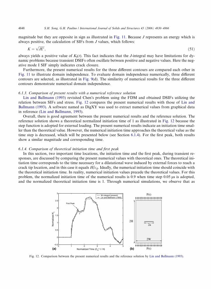
6.1.3. Comparison of present results with a numerical reference solution

Lin and Ballmann (1993) revisited Chen�s problem using the FDM and obtained DSIFs utilizing therelation between SIFs and stress. Fig. 12 compares the present numerical results with those of Lin andBallmann (1993). A software named as DigXY was used to extract numerical values from graphical datain reference (Lin and Ballmann, 1993).

Overall, there is good agreement between the present numerical results and the reference solution. Thereference solution shows a theoretical normalized initiation time of 1 as illustrated in Fig. 12 because thestep function is adopted for external loading. The present numerical results indicate an initiation time smal-ler than the theoretical value. However, the numerical initiation time approaches the theoretical value as thetime step is decreased, which will be presented below (see Section 6.1.4). For the first peak, both resultsshow a similar magnitude and corresponding time.

6.1.4. Comparison of theoretical initiation time and first peak

In this section, two important time locations, the initiation time and the first peak, during transient re-sponses, are discussed by comparing the present numerical values with theoretical ones. The theoretical ini-tiation time corresponds to the time necessary for a dilatational wave induced by external forces to reach acrack tip location, and in this case it equals H/cd. Ideally, the numerical initiation time should coincide withthe theoretical initiation time. In reality, numerical initiation values precede the theoretical values. For thisproblem, the normalized initiation time of the numerical results is 0.9 when time step 0.05 ls is adopted,and the normalized theoretical initiation time is 1. Through numerical simulations, we observe that as

(a) (b)0 1 2 3 4 5

–0.5

0

0.5

1

1.5

2

2.5

3

Normalized Time (Cd* t / H)

Nor

mal

ized

KI

M–integral (present)Lin and Ballmann (1993)

First Peak

P(t)

2a2H

2W

P(t)

Fig. 12. Comparison between the present numerical results and the reference solution by Lin and Ballmann (1993).

(a) (b)0.5 0.6 0.7 0.8 0.9 1 1.1

–0.2

0

0.2

0.4

0.6

0.8

1

1.2


Nor

mal

ized

KI

Time step: 0.05 μsTime step: 0.10 μsTime step: 0.30 μsTime step: 0.50 μs

Theoretical Initiation Time

T4 T3 T2 T1

T1 : Initiation time (Δt = 0.5 μs)




P(t)

2a2H

2W

P(t)

Fig. 13. Initiation time for 4 different time steps.


the time step decreases, the numerical initiation time approaches the theoretical value of 1 in Fig. 13. Thenormalized KI(t) for different time steps (0.05 ls, 0.1 ls, 0.3 ls and 0.5 ls) is plotted versus the normalizedtime in Fig. 13.

The first peak, indicated in Fig. 12, occurs in this problem when dilatational waves reach the crack tip,and generated Rayleigh waves travel to the opposite crack tip. At that instant, the Rayleigh waves causecompression at the crack tip and thus reduce the KI(t) values. The normalized theoretical time for this eventis 1.485 and the present numerical value is 1.523 for a time step of Dt = 0.05 ls. There is reasonably goodagreement between these numbers with a relative error less than 3%.

6.1.5. Sensitivity of numerical results with respect to time step size

For step loading, transient DSIFs are highly influenced by time step increment because the waves in-duced by this loading have a significant influence on crack tip fields, whereas for ramp loading, the cracktip fields are influenced primarily by the remote load. In the ramp loading, the load is always increasingwith time and, as a consequence, the magnitude of SIFs increases monotonically with time and shows littlevariation due to propagating waves. Therefore, SIFs are not very sensitive to the time step increment forramp loading.

Four different time steps, 0.05 ls, 0.1 ls, 0.3 ls and 0.5 ls, are chosen to investigate the influence of timestep on the DSIFs for step loading. As illustrated in Fig. 14, numerical results are highly influenced by thetime step. The abscissa and ordinate represent normalized time and normalized KI(t), respectively. Asthe time step decreases, the numerical results appear to converge. For the larger time steps, the differencebetween numerical results is especially pronounced near the peaks. This result indicates that for large timesteps, the transient response cannot be captured accurately.

6.1.6. Discussion of M-integral terms

The M-integral based on the non-equilibrium formulation is given by Eq. (32), i.e.,

M ¼Z

Aðraux


ik eikd1j

n oq;j dAþ

ZA�Cijkl;1e

auxkl eij þ raux

ij;j ui;1 þ q€uiuauxi;1

n oqdA. ð52Þ

The above expression consists of various terms which accounts for dynamic effects and material non-homo-geneity. Now, we will investigate and discuss the contribution of each term of the M-integral and its domainindependence. Let us define

0 1 2 3 4–1

–0.5

0

0.5

1

1.5

2

2.5

3

Normalized Time (Cd*t / H)

Nor

mal

ized

KI

Time step: 0.05 μsTime step: 0.10 μsTime step: 0.30 μsTime step: 0.50 μs

(a) (b) P(t)

2a2H

2W

P(t)

Fig. 14. Normalized KI(t) at the right crack tip for 4 different time steps: 0.05 ls, 0.1 ls, 0.3 ls and 0.5 ls.


Term 1 ¼Z

Araux

ij ui;1q;j dA; ð53Þ

Term 2 ¼Z

Arijuaux

i;1 q;j dA; ð54Þ

Term 3 ¼ �Z

Araux

ik eikd1jq;j dA; ð55Þ

Term 4 ¼ �Z

ACijkl;1e

auxkl eijq dA; ð56Þ

Term 5 ¼Z

Araux

ij;j ui;1qdA; ð57Þ

Term 6 ¼Z

Aq€uiuaux

i;1 q dA. ð58Þ

Terms 1, 2, and 3 are the same as those for homogeneous materials under quasi-static conditions. Terms 4and 5 arise due to material non-homogeneity, and Term 6 is due to dynamic effects.

For this simulation, the contours shown in Fig. 9(d) are used. Contour 1 includes 8 T6 and 24 Q8elements, contour 2 contains 54 T6 and 24 Q8 elements, and contour 3 has 54 T6 and 72 Q8 elements.Fig. 15(a)–(c) shows the contribution of each term to the normalized KI using contours 1, 2, and 3, respec-tively. The abscissa and ordinate represent normalized time and normalized KI(t), respectively. Terms 4 and5 are not included in Fig. 15 because they are zero for homogeneous materials. For all contours, the con-tributions of Terms 1 and 2 are higher than those of the other terms. Terms 1, 2, and 3 follow the trend ofthe total K, whereas Term 6 oscillates. Two important phenomena are observed from this simulation. Thefirst is the oscillatory nature of the contribution of Term 6 for different contours. The second is therelationship between initiation time and domain size.

For contour 1, illustrated in Fig. 15(a), the magnitude of Term 6 is small compared to that of otherterms. But as the domain size increases (from contour 1 to contour 3), the magnitude of Term 6 increasesoverall as illustrated in Fig. 16. It turns out that even if Term 6, which accounts for dynamic effects, is rel-atively small compared to other terms, the influence of this term in obtaining DSIFs becomes significant as

0 1 2 3 4–0.5

0

0.5

1

1.5

2

2.5

3


Nor

mal

ized

KI (

Con

tour

1)

Total DSIF Term 1

Term 2

Term 3

Term 6

0 1 2 3 41

0. 5

0

0.5

1

1.5

2

2.5

3

Nor

mal

ized

KI (

Con

tour

2)

Total DSIF Term 1

Term 2

Term 3 Term 6


0 1 2 3 4–1

–0.5

0

0.5

1

1.5

2

2.5

3


Nor

mal

ized

KI (

Con

tour

3)

Total DSIF Term 1

Term 2

Term 3

Term 6

(a) (b)

(c)

Fig. 15. Normalized KI(t) for three different contours: (a) contribution of each term for contour 1; (b) contribution of each term forcontour 2; (c) contribution of each term for contour 3.

(a) (b)0 1 2 3 4 5

–0.8

–0.6

–0.4

–0.2

0

0.2

0.4

0.6


Con

trib

utio

n of

term

6 to

nor

mal

ized

KI

Contour 1Contour 2Contour 3

P(t)

2a2H

2W

P(t)

Fig. 16. Contribution of Term 6 to normalized DSIFs for three different contours.


the domain size increases. Therefore, this term must be taken into account to satisfy domain independenceand to obtain correct DSIFs for dynamic problems.

(a) (b)0 1 2 3 4 5

0

0.5

1

1.5

2


Con

trib

utio

n of

term

1 to

nor

mal

ized

KI

Contour 1Contour 2Contour 3

P(t)

2a2H

2W

P(t)

Fig. 17. Contribution of Term 1 to normalized DSIFs for three different contours.


Dilatational waves reach the boundary of larger domains earlier than the boundary of small domains.We now investigate initiation times of individual terms for different domain sizes. Fig. 15 shows the con-tribution of each term for the three contours. Because contour 1 is very small, the difference between theinitiation time for each term and for the total DSIF is small (see Fig. 15(a)). However, for the larger con-tours 2 and 3 (see Fig. 15(b) and (c), respectively), it is clearly observed that Terms 1 and 6 initiate earlierthan the total DSIF. Moreover, Terms 1 and 6 initiate earlier, as domain size increases, as shown in Figs. 17and 16, respectively. However, the change of initiation time for the different domain sizes is not pronouncedfor Terms 2 and 3 (see Fig. 15). Notice that even if a few terms initiate earlier as the domain size increases,the initiation time of the total DSIF is independent of domain size, demonstrating domain independence(see Fig. 11).

6.2. Non-homogeneous CCT specimen

Dynamic fracture behavior of a homogeneous CCT specimen is examined thoroughly in Section 6.1. Inthis section, various material profiles are adopted to investigate fracture behavior in a non-homogeneousspecimen. First, domain independence of DSIFs for non-homogeneous material is verified. Then, behaviorof DSIFs at the right and left crack tips is explored.

Young�s modulus and mass density vary exponentially, such that E/q � constant, as given by

E ¼ EH expðb1xþ b2yÞ; ð59Þ

q ¼ qH expðb1xþ b2yÞ; ð60Þ

where EH and qH are Young�s modulus and mass density for homogeneous materials and b1 and b2 are non-homogeneity parameters along the x- and y-directions, respectively. When b1 and b2 are equal to zero, Eqs.(59) and (60) reflect homogeneous materials. A constant Poisson ratio of 0.3 is used. Plane strain elementswith 3 · 3 Gauss quadrature and consistent mass matrices are adopted for the bulk elements. A time step isDt = 0.1 ls. The geometry and the boundary conditions are identical to those of homogeneous specimenanalyzed in Section 6.1.1. Notice again that no other boundary conditions are prescribed except for theexternal loading.

6.2.1. Domain independence for non-homogeneous materials

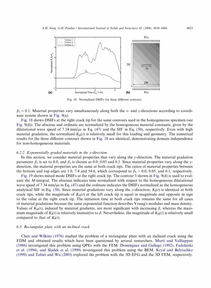
In this section, domain independence of the M-integral for non-homogeneous materials is demonstratednumerically. In order to employ severe material gradations, relatively high b values are chosen: b1 = 0.1 and

(a) (b)0 1 2 3

–1

0

1

2

3

4

Normalized Time (Cd* t /H)

Nor

mal

ized

KI &

KII

KII

KI

Contour 1 Contour 2 Contour 3

P(t)

2a2H

P(t)

2W

Fig. 18. Normalized DSIFs for three different contours.


b2 = 0.1. Material properties vary simultaneously along both the x- and y-directions according to coordi-nate system shown in Fig. 9(a).

Fig. 18 shows DSIFs at the right crack tip for the same contours used in the homogeneous specimen (seeFig. 9(d)). The abscissa and ordinate are normalized by the homogeneous material constants, given by thedilatational wave speed of 7.34 mm/ls in Eq. (47) and the SIF in Eq. (50), respectively. Even with highmaterial gradation, the normalized KII(t) is relatively small for this loading and geometry. The numericalresults for the three different contours shown in Fig. 18 are identical, demonstrating domain independencefor non-homogeneous materials.

6.2.2. Exponentially graded materials in the y-direction

In this section, we consider material properties that vary along the y-direction. The material gradationparameter b1 is set to 0.0, and b2 is chosen as 0.0, 0.05 and 0.1. Since material properties vary along the y-direction, the material properties are the same at both crack tips. The ratios of material properties betweenthe bottom and top edges are 1.0, 7.4 and 54.6, which correspond to b1 = 0.0, 0.05, and 0.1, respectively.

Fig. 19 shows mixed mode DSIFs at the right crack tip. The contour 3 shown in Fig. 9(d) is used to eval-uate the M-integral. The abscissa indicates time normalized with respect to the homogeneous dilatationalwave speed of 7.34 mm/ls in Eq. (47) and the ordinate indicates the DSIFs normalized as the homogeneousanalytical SIF in Eq. (50). Since material gradations vary along the y-direction, KI(t) is identical at bothcrack tips, while the magnitude of KII(t) at the left crack tip is equal in magnitude and opposite in signto the value at the right crack tip. The initiation time at both crack tips remains the same for all casesof material gradations because the same exponential function describes Young�s modulus and mass density.Values of KII(t), induced by material gradients, are more significant with increasing b, whereas the maxi-mum magnitude of KI(t) is relatively insensitive to b. Nevertheless, the magnitude of KII(t) is relatively smallcompared to that of KI(t).

6.3. Rectangular plate with an inclined crack

Chen and Wilkins (1976) studied the problem of a rectangular plate with an inclined crack using theFDM and obtained results which have been questioned by several researchers. Murti and Valliappan(1986) investigated this problem using QPEs with the FEM. Dominguez and Gallego (1992), Fedelinskiet al. (1994), and Sladek et al. (1999) investigated this problem using the BEM. Krysl and Belytschko(1999) and Tabiei and Wu (2003) explored the problem with the 3D EFG and the 3D FEM, respectively.

(a)

(b) (c)

0 1 2 3–0.5

0

0.5

1

1.5

2

2.5

3

Nor

mal

ized

KI (

Rig

ht C

rack

Tip

)

β2=0.0

β2=0.05 β

2=0.10

β1=0.0


0 1 2 3–0.1

–0.05

0

0.05

0.1

0.15

0.2

0.25

0.3

0.35

Nor

mal

ized

KII (

Rig

ht C

rack

Tip

)

β2=0.10

β2=0.05

β2=0.0

β1=0.0


2H2a

P(t)

P(t)

2W

Fig. 19. DSIFs for different material gradations along the y-direction: (a) normalized KI(t) at the right crack tip; (b) normalized KII(t)at the right crack tip; (c) functionally graded CCT specimen.


Consider an inclined crack of length 2a = 14.14 mm in a rectangular plate of width 2W = 30 mm andheight 2H = 60 mm, as shown in Fig. 20(a). Fig. 20(b) and (c) illustrate the mesh for the whole geometry,and the four contours employed at each crack tip. The entire mesh consists of 206 Q8 and 198 T6 elements.Contour 1 includes only 8 T6 elements, contour 2 encloses 8 T6 and 24 Q8 elements, contour 3 contains 31T6 and 24 Q8 elements, and contour 4 has 77 T6 and 26 Q8 elements. To obtain a reasonable mesh reso-lution near the crack tips, 4 rings and 8 sectors of elements are used. The external force, p(t), is appliedinstantaneously to both the top and bottom edges with a step function (see Fig. 10). No other boundaryconditions are prescribed.

For the non-homogeneous case, Young�s modulus and mass density vary exponentially along the x- andy-directions, such that E/q � constant, according to

E ¼ EH expðb1xþ b2yÞ; ð61Þq ¼ qH expðb1xþ b2yÞ; ð62Þ

where EH and qH are Young�s modulus and mass density for homogeneous material, and b1 and b2 are thematerial non-homogeneity parameters that describe material gradation. When b1 and b2 equal zero,homogeneous material properties are recovered. A constant Poisson�s ratio of 0.3 is employed. Plane strainelements with 3 · 3 Gauss quadrature are used. A time step is Dt = 0.1 ls.

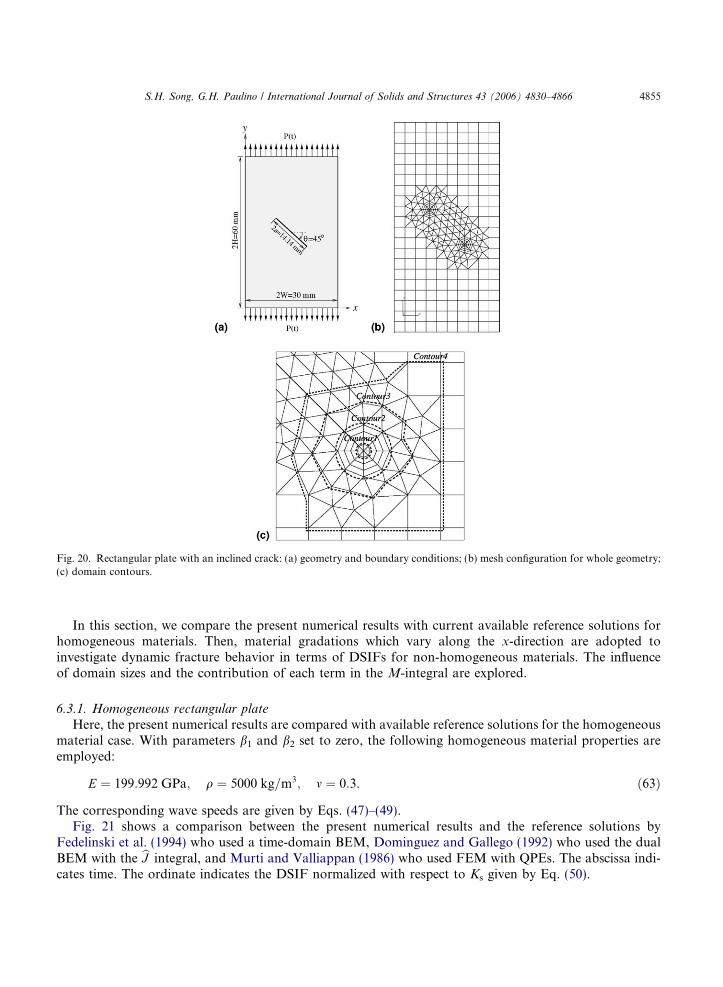
Fig. 20. Rectangular plate with an inclined crack: (a) geometry and boundary conditions; (b) mesh configuration for whole geometry;(c) domain contours.


In this section, we compare the present numerical results with current available reference solutions forhomogeneous materials. Then, material gradations which vary along the x-direction are adopted toinvestigate dynamic fracture behavior in terms of DSIFs for non-homogeneous materials. The influenceof domain sizes and the contribution of each term in the M-integral are explored.

6.3.1. Homogeneous rectangular plate

Here, the present numerical results are compared with available reference solutions for the homogeneousmaterial case. With parameters b1 and b2 set to zero, the following homogeneous material properties areemployed:

E ¼ 199:992 GPa; q ¼ 5000 kg=m3; m ¼ 0:3. ð63Þ

The corresponding wave speeds are given by Eqs. (47)–(49).Fig. 21 shows a comparison between the present numerical results and the reference solutions by

Fedelinski et al. (1994) who used a time-domain BEM, Dominguez and Gallego (1992) who used the dualBEM with the bJ integral, and Murti and Valliappan (1986) who used FEM with QPEs. The abscissa indi-cates time. The ordinate indicates the DSIF normalized with respect to Ks given by Eq. (50).

0 5 10 15 20–0.2

0

0.2

0.4

0.6

0.8

1

1.2

1.4

1.6

Time (μs)

Nor

mal

ized

KI

Dominguez & Gallego (1992)Fedelinski et al. (1994)Murti & Valliappan (1986)M–integral (present)

P(t)

P(t)

(a) (b)

Fig. 21. Numerical comparison between the present results and the reference solutions (Murti and Valliappan, 1986; Dominguez andGallego, 1992; Fedelinski et al., 1994).


The reference results plotted here are obtained from graphical data using special-purpose software. Upto 10 ls, the difference between the results is not significant. After that time, the discrepancy among theresults becomes greater when the influence of reflected waves becomes significant. This implies that the var-ious numerical schemes differently predict the transient fracture response which is highly influenced bypropagating waves reflected from the boundary and crack surfaces. Up to 10 ls, the present results matchwell with the solution by Dominguez and Gallego (1992), and afterwards, the present results are within therange of the other solutions. Moreover, the present results show more oscillations (small amplitude) thanthe other solutions.

6.3.2. Exponentially graded materials in the x-direction

Material properties varying along the x-direction are employed to investigate DSIFs for non-homoge-neous materials. The material gradation parameter b1 is chosen as 0.0, 0.05, 0.1 and 0.15, and b2 is setto zero. The ratio of material properties at the left and right boundaries ranges from 1.0 to 90.0. Althoughthis high material ratio, i.e., 90, is not realistic, such high material gradation is adopted in order to clearlyobserve the influence of different material profiles on the variation of DSIFs.

Fig. 22 illustrates the variation of mixed mode DSIFs at the left and right crack tip locations. The ordinateindicates normalized DSIFs and the abscissa indicates time up to 20 ls. Both crack tips have the same initi-ation time for the different material gradations because Young�s modulus and mass density follow the sameexponential function. As the parameter b1 increases, the magnitude of KI(t) at the right crack tip increases. Atthe left crack tip, up to around 15 ls, the magnitude of KI(t) is larger for smaller values of b1 and after thattime, the magnitude of KI(t) becomes smaller for smaller values of b1. For KII(t), as b1 increases, the absolutemagnitude of KII(t) at both crack tips first decreases and then increases. Moreover, the absolute value of max-imum KI(t) at the right crack tip is higher than that at the left crack tip as b1 increases. This behavior isreasonable because the material property values at the right crack tip are higher than those at the left cracktip.

6.3.3. Discussion of M-integral terms for non-homogeneous materials

In Section 6.1.6, the contribution of each term was explored thoroughly for homogeneous materials. Toaccount for material non-homogeneity in the current specimen, the M-integral includes Terms 4 and 5. Inthis section, we examine the influence of each term of the M-integral. Also, we discuss the influence ofdomain size on the magnitude of Terms 4, 5 and 6, which account for material non-homogeneity and

0 2 4 6 8 10 12 14 16 18 200

0.2

0.4

0.6

0.8

1

1.2

1.4

Time (μs)

Nor

mal

ized

KI o

f Lef

t Cra

ck T

ip

β1=0.15

β1=0.10

β1=0.05

β1=0.00

0 2 4 6 8 10 12 14 16 18 200

0.5

1

1.5

2

2.5

3

Time (μs)

Nor

mal

ized

KI o

f Rig

ht C

rack

Tip β

1=0.15

β1=0.10

β1=0.05

β1=0.0

0 2 4 6 8 10 12 14 16 18 20–1.6

–1.4

–1.2

–1

0. 8

0. 6

0. 4

0. 2

0

0.2

0.4

Time (μs)

Nor

mal

ized

KII o

f Lef

t Cra

ck T

ip

β1=0.15

β1=0.10

β1=0.05

β1=0.0

0 2 4 6 8 10 12 14 16 18 20–2

–1.5

–1

0. 5

0

0.5

Time (μs)

Nor

mal

ized

KII o

f Rig

ht C

rack

Tip

β1=0.0

β1=0.05

β1=0.10

β1=0.15

(a) (b)

(c) (d)

Fig. 22. Mixed mode DSIFs: (a) normalized KI(t) at the left crack tip; (b) normalized KI(t) at the right crack tip; (c) normalized KII(t)at the left crack tip; (d) normalized KII(t) at the right crack tip.


dynamic effects. The four different contours illustrated in Fig. 20(c) are used. The value of b1 is chosen as0.1 and b2 is chosen as zero, i.e., (b1,b2) = (0.1,0.0). The element type, numerical schemes and time step arethe same as in the homogeneous case for this specimen.

Fig. 23 shows the contribution of individual terms to normalized DSIFs, KI(t)/Ks and KII(t)/Ks where Ks

is given by Eq. (50), versus time at both the right and left crack-tip locations for the four different contours.The different terms are given by Eqs. (53)–(58). For contour 1, Terms 4 and 5, representing non-homoge-neous material effects, and Term 6, accounting for dynamic effects, are small. This shows numerically thatthe influence of inertia and material non-homogeneity on DSIFs is almost negligible very near the crack tip.Overall, the trend and contribution of Terms 1 and 2 are similar for all contours. During the time period upto 20 ls, Terms 1, 2, 3 and 5 are positive, Term 4 is negative, and Term 6 oscillates. Notice that even thoughthe contribution of each term varies for different contours, the total K is the same for each contour, dem-onstrating domain independence. We now discuss two important observations: (1) The effects of domainsize on non-homogeneous and dynamic terms; (2) the relationship between initiation time and domain size.

Fig. 24(a)–(c), respectively, illustrate the contribution of Terms 4, 5 and 6 for different domain sizes. Aswe increase the domain size from contour 1 to contour 4, the contribution of Terms 4 and 5, which accountfor material non-homogeneity, increases and Term 6, which represents dynamic effects, increases in mag-nitude as well. Therefore, if we neglect these terms in evaluating the M-integral for non-homogeneous

0 2 4 6 8 10 12 14 16 18 20–0.5

0

0.5

1

1.5

2

2.5

Time (μs)

Nor

mal

ized

KI (

Con

tour

1) Total DSIF

Term 1

Term 2Term 3

Term 4Term 6

Term 5

0 2 4 6 8 10 12 14 16 18 20~0.5

0

0.5

1

1.5

2

2.5

Time (μs)

Nor

mal

ized

KI (

Con

tour

2)

Total DSIF Term 1

Term 2

Term 3

Term 5

Term 6 Term 4

0 2 4 6 8 10 12 14 16 18 20–0.5

0

0.5

1

1.5

2

2.5

Time (μs)

Nor

mal

ized

KI (

Con

tour

3)

Total DSIF Term 1

Term 2 Term 3

Term 4 Term 5

Term 6

0 2 4 6 8 10 12 14 16 18 20–0.5

0

0.5

1

1.5

2

2.5

Time (μs)

Nor

mal

ized

KI (

Con

tour

4)

Total DSIF Term 1

Term 2 Term 3

Term 4 Term 5

Term 6

(a) (b)

(c) (d)

Fig. 23. Contribution of individual terms to the DSIFs for different contours: (a) contribution of each term for contour 1; (b)contribution of each term for contour 2; (c) contribution of each term for contour 3; (d) contribution of each term for contour 4.


cracked specimen under dynamic loadings, domain independence is violated and accuracy worsens as thedomain size increases.

Fig. 25(a) and (b) shows the initiation time of each term for contours 1 and 4, respectively. For bothfigures, the abscissa indicates time from 1.5 ls to 3.5 ls and the ordinate indicates normalized KI(t). Forcontour 1, each term and the total DSIF initiate at the same time denoted by T in Fig. 25(a). For contour4, however, the initiation time of Terms 1, 2, 3 and 6, T1 in Fig. 25(b), is less than that of total DSIF, i.e., T.It is reasonable because waves reach the boundary of larger domains earlier than the boundary of smalldomains. On the contrary, initiation time T of Terms 4 and 5 and total DSIF are almost identical. Noticethat even though a few terms initiate early, the initiation time of the total DSIF for different contours is thesame satisfying domain independence.

6.4. Rectangular plate with cracks emanating from a circular hole

Fedelinski et al. (1994) used the dual BEM and bJ integral to determine DSIFs in a rectangular plate withcracks emanating from a circular hole. A decomposition procedure was employed for mode mixity. Variousangles which range from 0� to 60� were adopted to investigate fracture behavior in terms of the variation ofDSIFs. In this study, crack angles of 30� are chosen to investigate the influence of material gradation onDSIFs for non-homogeneous materials.

0 2 4 6 8 10 12 14 16 18 20–0.5

–0.45

–0.4

–0.35

–0.3

–0.25

–0.2

–0.15

–0.1

–0.05

0

Time (μs)

Con

trib

utio

n of

Ter

m 4

to n

orm

aliz

ed K

I

Contour 1Contour 2

Contour 3

Contour 4

0 2 4 6 8 10 12 14 16 18 20–0.1

0

0.1

0.2

0.3

0.4

0.5

0.6

Time (μs)

Con

trib

utio

n of

Ter

m 5

to n

orm

aliz

ed K

I

Contour 4 Contour 3

Contour 2

Contour 1

0 2 4 6 8 10 12 14 16 18 20–0.3

–0.2

–0.1

0

0.1

0.2

0.3

0.4

Time (μs)

Con

trib

utio

n of

Ter

m 6

to n

orm

aliz

ed K

I

Contour 1 Contour 2

Contour 3 Contour 4

(a) (b)

(c)

Fig. 24. The influence of domain size on the contribution of each term to DSIFs: (a) Term 4 contribution; (b) Term 5 contribution; (c)Term 6 contribution.

1.5 2 2.5 3 3.5–0.02

0

0.02

0.04

0.06

0.08

0.1

0.12

Time (μs)

Nor

mal

ized

KI (

Con

tour

1)

T

Total DSIF Term 1

Term 2Term 3

Term 4, 5, 6

1.5 2 2.5 3 3.5–0.15

–0.1

–0.05

0

0.05

0.1

0.15

0.2

0.25

Time (μs)

Nor

mal

ized

KI (

Con

tour

4)

Term 1

Term 3

Total DSIF

Term 5Term 4

Term 2

Term 6

T1

T

o

(a) (b)

Fig. 25. Relationship between domain size and initiation time of each term in the M-integral: (a) normalized KI(t) at right crack tip forcontour 1; (b) normalized KI(t) at right crack tip for contour 4.


(c) (d)

x

P(t)

P(t)

2W=30 mm

=30θ2a=15 mm

r=3.75 mm

2H=

60 m

m

y

(a) (b)

Fig. 26. Rectangular plate with cracks emanating from a circular hole: (a) geometry and boundary conditions; (b) mesh configurationfor whole geometry; (c) mesh details for both crack tip regions; (d) mesh details for the right crack tip (12 sectors and 4 rings).


Fig. 26(a) illustrates a rectangular finite plate with a width 2W = 30 mm and a height 2H = 60 mm con-taining a hole of radius r = 3.75 mm. Two cracks extend from the hole, and the length between the twocrack tips is 15 mm. The cracks are inclined at 30� clockwise from horizontal. Fig. 26(b)–(d) shows the meshconfigurations for the whole geometry, and mesh detail for near the hole and the crack tips. A crack tiptemplate of 12 sectors and 4 rings of elements provide sufficient mesh refinement around the crack tip re-gions, which is crucial to obtain reliable numerical results. Step loading, which is illustrated in Fig. 10, isapplied to both the top and bottom edges. In this mesh, 1350 Q8 and 204 T6 plane strain elements are usedwith 3 · 3 Gauss quadrature. A time step is Dt = 0.1 ls.

6.4.1. Homogeneous plate

A comparison between the present numerical results and a reference solution is carried out. For thehomogeneous plate, the material properties described in Section 6.3.1 are used. The corresponding wavespeeds are given by Eqs. (47)–(49).

Fig. 27 shows the comparison between present numerical results at the right crack tip and the solutionsby Fedelinski et al. (1994). The reference results plotted here are obtained from graphical data using

0 5 10 15 20–1.5

–1

–0.5

0

0.5

1

1.5

2

2.5

Time (μs)

Nor

mal

ized

KI &

KII

KI of numerical results

KI of reference solutions

KII of numerical results

KII of reference solutions

(a) (b)

Fig. 27. The comparison between the present numerical results and reference solutions (Fedelinski et al., 1994).


special-purpose software. The abscissa indicates time up to 20 ls. The DSIFs are normalized by Ks given inEq. (50). The values of KII(t) in Fedelinski et al. (1994) are positive, while the present numerical values ofKII(t) are negative up to around 18 ls in Fig. 27. This might be due to different sign convention in shear.The same magnitude but opposite sign of the KII(t) in the reference solution is compared with the presentnumerical values of KII(t). Greater but acceptable difference is found for KI(t) values than for KII(t) values.

Table 3Material properties and dilatational wave speed along the left and right edges

Young�s modulus (MPa) Mass density (kg/m3) Longitudinal wave speed (mm/ls)

Left edge 3811 948 2.33Right edge 11,130 1812 2.88

0 5 10 15 20 25 30 35 40–2

–1.5

–1

–0.5

0

0.5

1

1.5

2

2.5

3

Time (μs)

Nor

mal

ized

KI &

KII

KI at right crack tip

KI at left crack tip

KII at left crack tip

KII at right crack tip

(a) (b)

Fig. 28. Normalized mixed-mode DSIFs at both the left and right crack tips for non-homogeneous materials.


The difference may be due to different numerical schemes, different domain discretization, and different con-servation integrals; bJ integral and M-integral. Overall, the present numerical results agree well with thisreference solution.

6.4.2. Non-homogeneous plateIn this example, real non-homogeneous material properties prepared by Rousseau and Tippur (2001) are

adopted here to investigate fracture behavior. They prepared three point bending specimens made of epoxyand solid soda-lime glass spheres. The material properties of the current specimen possess the values pro-vided in Rousseau and Tippur (2001) and assume linear variation of material properties in the x-direction,which is described by

EðxÞ ¼ ð244xþ 7471Þ ðMPaÞ; ð64ÞqðxÞ ¼ ð28:8xþ 1380Þ ðkg=m3Þ. ð65Þ

A constant Poisson�s ratio of 0.3 is used. Table 3 shows material properties and the corresponding dilata-tional wave speed along the left edge and the right edge. Notice that the longitudinal wave speed is differentat each location due to the different variation between Young�s modulus and mass density.

Normalized mixed-mode DSIFs at both the right and left crack tip locations are plotted versus time inFig. 28. The ordinate indicates DSIFs normalized by Ks (see Eq. (50)) and the abscissa is time up to 40 ls.Since initiation time of DSIFs depends on the dilatational wave speed, first the DSIFs at the right crack tipinitiate, and then, the DSIFs at the left crack tip initiate as shown in Fig. 28. At any given time of the tran-sient response, the magnitude of KI(t) at the right crack tip is higher than that at the left crack tip for thenon-homogeneous case. This is due to the fact that the values of material properties at the right crack tipare higher than those at the left crack tip.

7. Conclusion

Dynamic fracture behavior for both homogeneous and non-homogeneous materials is examined thor-oughly in this study. The M-integral is superior to the DCT in terms of accuracy, and unlike the standardJ-integral, it yields mixed-mode SIFs directly. Thus, the M-integral is extended to incorporate the materialnon-homogeneity and dynamic effects. Notice that Williams� solution (1957) is employed as dynamic auxil-iary fields because the asymptotic singular stress fields in non-homogeneous materials under dynamic condi-tion are shown to have similar behaviors with those in homogeneous materials under quasi-static condition(Eischen, 1987; Freund, 1998; Freund and Clifton, 1974; Nilsson, 1974; Parameswaran and Shukla, 1999).The non-equilibrium formulation of the M-integral is employed here to evaluate SIFs for both static and dy-namic cases. The research code, which has been developed using the implicit time scheme and the M-integralwith graded elements by means of the GIF (Kim and Paulino, 2002a), is verified using benchmark problems.Using the verified code, fracture problems are presented and discussed. In non-homogeneous media, varia-tion of DSIFs is hard to be generalized because it is highly dependent upon geometry, material gradation andboundary conditions. However, as seen in the previous examples, e.g., Fig. 22, the magnitude of DSIFs at thecrack tip located in the stiffer part increases overall, as material gradation increases, i.e., b increases.

The major contributions of this study can be summarized as follows:

• The M-integral based on the non-equilibrium formulation is derived to account for material non-homo-geneity and dynamic effects.

• The mode I and mixed mode DSIFs for both homogeneous and non-homogeneous materials are eval-uated using the M-integral.


• The domain independence of the M-integral is assessed numerically for both homogeneous and non-homogeneous materials under dynamic loading.

• Fracture behavior is investigated thoroughly for homogeneous and non-homogeneous materials underdynamic loading, including the influence of material gradation on variations of DSIFs, the relationbetween initiation time and the domain size, and the contribution of each distinct term in the M-integral.

Acknowledgement

We are grateful to the support from the National Science Foundation (NSF) through the GOALI pro-ject CMS 0219566 (Program Manager, P. N. Balaguru). Any opinions expressed herein are those of thewriters and do not necessarily reflect the views of the sponsors.

Appendix A. Numerical implementation details

The displacement field of Williams� (1957) solution can be rewritten as

u‘ðr; hÞauxi ¼ Kaux

I

ltip

gIi ðr; hÞ þ

KauxII

ltip

gIIi ðr; hÞ ði ¼ 1; 2Þ; ð66Þ

where superscript ‘ means local coordinate. The derivatives of auxiliary displacements with respect to theglobal coordinate systems are calculated as follows (k = 1,2):

ugðr; hÞauxi;k ¼

ougðr; hÞauxi

oX k¼ ougðr; hÞaux

i

oror

oX kþ ougðr; hÞaux

i

ohohoX k

; ð67Þ

where

ugðr; hÞaux1

ugðr; hÞaux2

� �¼

cos a � sin a

sin a cos a

u‘ðr; hÞaux

1

u‘ðr; hÞaux2

( )ð68Þ

and

oroX k¼ or

ox1

ox1

oX kþ or

ox2

ox2

oX k;

ohoX k¼ oh

ox1

ox1

oX kþ oh

ox2

ox2

oX k; ð69Þ

with

or=ox1 ¼ cos h; or=ox2 ¼ sin h;

oh=ox1 ¼ � sin h=r; oh=ox2 ¼ cos h=r;

ox1=oX 1 ¼ cos a; ox1=oX 2 ¼ sin a;

ox2=oX 1 ¼ � sin a; ox2=oX 2 ¼ cos a.

ð70Þ

As illustrated in Fig. 4, a is the angle between global and local coordinates, r is the radial distance, and h isthe angle between local and the point where field quantities are obtained. Notice that (x1,x2) and (X1,X2)indicate local and global coordinates, respectively.

Due to the non-equilibrium formulation, the auxiliary strain field is obtained using the compatibilitycondition as

egðr; hÞauxij ¼

1

2ðugðr; hÞaux

i;j þ ugðr; hÞauxj;i Þ; ð71Þ

where ug(r,h)i,j is obtained using Eq. (66).


The auxiliary stress is evaluated using the constitutive relationship

rgðr; hÞauxij ¼ CijklðxÞegðr; hÞaux

kl . ð72Þ

The material properties used in the constitutive tensor are computed using the isoparametric formulation(Kim and Paulino, 2002a).

The derivative of the auxiliary stress is given by

ðrgðr; hÞauxij Þ;j ¼ ðCijklðxÞegðr; hÞaux

kl Þ;j ¼ Cijkl;jegðr; hÞaux

kl þ Cijklegðr; hÞaux

kl;j ; ð73Þ

where the derivative of auxiliary fields with respect to global coordinates, egðr; hÞauxkl;j , is evaluated as

follows:

egðr; hÞauxij;k ¼

oegðr; hÞauxij

oX k¼

oegðr; hÞauxij

oror

oX kþ

oegðr; hÞauxij

ohohoX k

. ð74Þ

In computing Eq. (74), the Eqs. (69) and (70) are used.

References

ABAQUS, 2004. Version 6.4, H.K.S. Inc., Pawtucket, RI.Anderson, T.L., 1995. Fracture Mechanics: Fundamentals and Application. CRC, Boca Raton.Aoki, S., Kishimoto, K., Kondo, H., Sakata, M., 1978. Elastodynamic analysis of crack by finite element method using singular

element. International Journal of Fracture 14 (1), 59–67.Belytschko, T., Lu, Y.Y., Gu, L., Tabbara, M., 1995. Element free Galerkin methods for static and dynamic fracture. International

Journal of Solids and Structures 32 (17/18), 2547–2570.Brickstad, B., 1983. A FEM analysis of crack arrest experiments. International Journal of Fracture 21 (3), 177–194.Bui, H.D., 1983. Associated path independent J-integrals for separating mixed modes. Journal of the Mechanics and Physics of Solids

31 (6), 439–448.Buttlar, W.G., Paulino, G.H., Song, S.H., 2005. Application of graded finite elements for asphalt pavement analysis. ASCE Journal of

Engineering Mechanics, in press.Chen, Y.M., 1975. Numerical computation of dynamic stress intensity factors by a Lagrangian finite-difference method (the HEMP

code). Engineering Fracture Mechanics 7 (4), 653–660.Chen, Y.M., Wilkins, M.L., 1976. Stress analysis of crack problems with a three dimensional time dependent computer program.

International Journal of Fracture 12 (4), 607–617.Dolbow, J., Gosz, M., 2000. On the computation of mixed-mode stress intensity factors in functionally graded materials. International

Journal of Solids and Structures 39 (9), 2557–2574.Dominguez, J., Gallego, R., 1992. Time domain boundary element method for dynamic stress intensity factor computations.

International Journal for Numerical Methods in Engineering 33 (3), 635–647.Eftis, J., Subramonian, N., Liebowitz, H., 1977. Crack border stress and displacement equation revisited. Engineering Fracture

Mechanics 9 (1), 189–210.Eischen, J.W., 1987. Fracture of non-homogeneous materials. International Journal of Fracture 34 (1), 3–22.Enderlein, M., Ricoeur, A., Kuna, M., 2003. Comparison of finite element technique for 2D and 3D crack analysis under impact

loading. International Journal of Solids and Structures 40 (13–14), 3425–3437.Fedelinski, P., 2004. Boundary element method in dynamic analysis of structures with cracks. Engineering Analysis with Boundary

Elements 28 (9), 1135–1147.Fedelinski, P., Aliabadi, M.H., Rooke, D.P., 1994. The dual boundary element method: bJ -integral for dynamic stress intensity factors.

International Journal of Fracture 65 (4), 369–381.Freund, L.B., 1998. Dynamic Fracture Mechanics. Cambridge University Press, Cambridge.Freund, L.B., Clifton, R.J., 1974. On the uniqueness of plane elastodynamic solutions for running cracks. Journal of Elasticity 4 (4),

293–299.Fung, Y.C., 1965. Foundation of Solid Mechanics. Prentice-Hall, Englewood Cliffs, NJ.


Hughes, T.J.R., 1987. The Finite Element Method: Linear Static and Dynamic Finite Element Analysis. Prentice-Hall, New Jersey.Kim, J.-H., Paulino, G.H., 2002a. Isoparametric graded finite elements for non-homogeneous isotropic and orthotropic materials.

ASME Journal of Applied Mechanics 69 (4), 502–514.Kim, J.-H., Paulino, G.H., 2002b. Finite element evaluation of mixed mode stress intensity factors in functionally graded materials.

International Journal for Numerical Methods in Engineering 53 (8), 1903–1935.Kim, J.-H., Paulino, G.H., 2003a. T-stress, mixed-mode stress intensity factors, and crack initiation angles in functionally graded

materials: a unified approach using the interaction integral method. Computer Methods in Applied Mechanics and Engineering 192(11/12), 1463–1494.

Kim, J.-H., Paulino, G.H., 2003b. An accurate scheme for mixed-mode fracture analysis of functionally graded materials using theinteraction integral and micromechanics models. International Journal for Numerical Methods in Engineering 58 (10), 1457–1497.

Kim, J.-H., Paulino, G.H., 2005. Consistent formulations of the interaction integral method for fracture of functionally gradedmaterials. ASME Journal of Applied Mechanics 72 (3), 351–364.

Kishimoto, K., Aoki, S., Sakata, M., 1980. Dynamic stress intensity factors using J-integral and finite element method. EngineeringFracture Mechanics 13 (2), 387–394.

Konda, N., Erdogan, F., 1994. The mixed mode crack problem in a non-homogeneous elastic medium. Engineering FractureMechanics 47 (4), 533–545.

Krysl, P., Belytschko, T., 1999. The element free Galerkin method for dynamic propagation of arbitrary 3-D cracks. InternationalJournal for Numerical Methods in Engineering 44 (6), 767–800.

Lee, Y.J., Freund, L.B., 1990. Fracture initiation due to asymmetric impact loading of an edge cracked plate. ASME Journal ofApplied Mechanics 57 (1), 104–111.

Lin, X., Ballmann, J., 1993. Re-consideration of Chen�s problem by finite difference method. Engineering Fracture Mechanics 44 (5),735–739.

Moran, B., Shih, F.C., 1987. Crack tip and associated domain integrals from momentum and energy balance. Engineering FractureMechanics 27 (6), 615–642.

Murti, V., Valliappan, S., 1986. The use of quarter point element in dynamic crack analysis. Engineering Fracture Mechanics 23 (3),585–614.

Newmark, N.M., 1959. A method of computation for structural dynamics. ASCE Journal of Engineering Mechanics 85 (EM3, Part 1),67–94.

Nilsson, F., 1974. A note on the stress singularity at a non-uniformly moving crack tip. Journal of Elasticity 4 (1), 73–75.Parameswaran, V., Shukla, A., 1999. Crack tip stress fields for dynamic fracture in functionally gradient materials. Mechanics of

Materials 31 (9), 579–596.Raju, I.S., Shivakumar, K.N., 1990. An equivalent domain integral method in the two dimensional analysis of mixed mode crack

problems. Engineering Fracture Mechanics 37 (4), 707–725.Rao, B.N., Rahman, S., 2003. Mesh-free analysis of cracks in isotropic functionally graded materials. Engineering Fracture Mechanics

70 (1), 1–27.Rice, J.R., 1968. A path-independent integral and the approximate analysis of strain concentration by notches and cracks. ASME

Journal of Applied Mechanics 35 (2), 379–386.Rousseau, C.-E., Tippur, H.V., 2001. Dynamic fracture of compositionally graded materials with cracks along the elastic gradient:

experiment and analysis. Mechanics of Materials 33 (7), 403–421.Santare, M.H., Lambros, J., 2000. Use of graded finite elements to model the behavior of non-homogeneous materials. Journal of

Applied Mechanics—Transactions ASME 67 (4), 819–822.Santare, M.H., Thamburaj, P., Gazonas, G.A., 2003. The use of graded finite elements in the study of elastic wave propagation in

continuously non-homogeneous materials. International Journal of Solids and Structures 40 (21), 5621–5634.Shih, C.F., deLorenzi, H.G., German, M.D., 1976. Crack extension modeling with singular quadratic isoparametric elements.

International Journal of Fracture 12 (4), 647–651.Sladek, J., Sladek, V., Fedelinski, P., 1997. Integral formulation for elastodynamic T-stresses. International Journal of Fracture 84 (2),

103–116.Sladek, J., Sladek, V., Fedelinski, P., 1999. Computation of the second fracture parameter in elastodyanamics by the boundary element

method. Advances in Engineering Software 30 (9/11), 725–734.Song, S.H., 2003. Dynamic stress intensity factors for homogeneous and non-homogeneous materials using the interaction integral

method, Master Thesis, Department of Civil and Environmental Engineering, University of Illinois at Urbana-Champaign.Tabiei, A., Wu, J., 2003. Development of the DYNA3D simulation code with automated fracture procedure for brick elements.

International Journal for Numerical Methods in Engineering 57 (14), 1979–2006.Whirley, R.G., Engelmann, B.E., 1993. DYNA3D User Manual, Lawrence Livermore National Laboratory.Williams, M.L., 1957. On the stress distribution at the base of a stationary crack. ASME Journal of Applied Mechanics 24 (1),

109–114.


Wu, C.-C., He, P., Li, Z., 2002. Extension of J integral to dynamic fracture of functional graded material and numerical analysis.Computers and Structures 80 (5/6), 411–416.

Yau, J.F., Wang, S.S., Corten, H.T., 1980. A mixed mode crack analysis of isotropic solids using conservation laws of elasticity. ASMEJournal of Applied Mechancis 47 (2), 335–341.

Zhang, Ch., 2002. A 2D hypersingular time domain traction BEM for transient elastodynamic crack analysis. Wave Motion 35 (1),17–40.

Dynamic stress intensity factors for homogeneous and ... · Dynamic stress intensity factors for...

Documents

Transcript of Dynamic stress intensity factors for homogeneous and ... · Dynamic stress intensity factors for...