Dynamic stability of vortex solutions of Ginzburg-Landau ...

Commun. Math. Phys. 180, 389-428 (1996) Communications in Mathematical

Physics �9 Springer-Verlag 1996

Dynamic Stability of Vortex Solutions of Ginzburg-Landau and Nonlinear Schr6dinger Equations

M . I . W e i n s t e i n 1, J . X i n 2

1 Department of Mathematics, University of Michigan, Ann Arbor, MI 48109, USA 2 Department of Mathematics, University of Arizona, Tucson, AZ 85721, USA

Received: 1 November 1995/Accepted: 15 February 1996

Abstract: The dynamic stability of vortex solutions to the Ginzburg-Landau and nonlinear Schr6dinger equations is the basic assumption of the asymptotic particle plus field description of interacting vortices. For the Ginzburg-Landau dynamics we prove that all vortices are asymptotically nonlinearly stable relative to small radial perturbations. Initially finite energy perturbations of vortices decay to zero in LP(IR 2) spaces with an algebraic rate as time tends to infinity. We also prove that under general (nonradial) perturbations, the plus and minus one-vortices are linearly dynamically stable in L2; the linearized operator has spectrum equal to ( - c % 0 ] and generates a Co semigroup of contractions on L2(IR2). The nature of the zero energy point is clarified; it is resonance, a property related to the infinite energy of planar vortices. Our results on the linearized operator are also usbd to show that the plus and minus one-vortices for the Schr6dinger (Hamiltonian) dynamics are spectrally stable, i.e. the linearized operator about these vortices has (L 2) spectrum equal to the imaginary axis. The key ingredients of our analysis are the Nash-Aronson estimates for obtaining Gaussian upper bounds for fundamental solutions of parabolic operators, and a combination of variational and maximum principles.

1. Introduct ion

In this paper, we study the dynamic stability of vortex solutions of the Ginzburg- Landau and nonlinear Schr6dinger equations:

u t = A u -c- (1 - lul2)u -- ~5~ &7 '

(1.1)

- i u t = Au + (1 - lul2)u - 6E & 7

(1.2)

Here, u = u(t,x) is a complex valued function defined for each t > 0 and x (x~,x2) E IR 2. A = 02 + 02 denotes the two-dimensional Laplacian. The energy XI X2

390 M.I. Weinstein, J. Xin

functional

R 2 (1.3)

The Ginzburg-Landau equation arises in the theory of superconductivity; see [4, 11,20] and references therein. The nonlinear Schr6dinger equation is a basic model for superfluids; see, for example, [7, 10,24, 15, 12]. These equations also play a central role as universal envelope equations for bifurcation problems and pattern dynamics; see, for example, [25].

Equations (1.1) and (1.2) admit vortex solutions. These are solutions of the form:

~Pn(x) = Un(r)e inO, n = 4-1, • . . . . ,

g~(0) = 0, gn(+oc) = 1, (1.4)

where (r, 0) denote the polar coordinates IR 2. The functions ~gn(x) define complex vector fields in the plane: (xl,x2)~-+ (Real ~vn, Imag ~P,), whose zeros are called vortices or defects. Since the evolution equations (1.1) and (1.2) define continuous deformations of the complex vector field, u( . ,x), if the initial total winding number or circulation at infinity is different from zero, one expects a principal feature of the dynamics to be the interaction of vortices or local flow fields organized around the zeros of u(t ,x) . A description of the dynamics of an ensemble of spatially separated vortices, each having the local structure (1.4), is therefore of fundamental interest.

The systematic study of this problem was initiated by Neu [24]; see also the work of Pismen and Rubinstein [30], and E [11]. In these works, the regime of small e, the ratio of vortex core size to the separation distance between vortices, is considered. In addition to his asymptotic analysis, Neu [24] presents numerical evidence for the stability of one-vortices and the fission instability of n-vortices (Inl __> 2). This motivates the underlying assumption of these asymptotic studies that the one-vortices (Inl = 1 in (1.4)) are stable. For e small, a solution is sought in the form of a product of one-vortices plus small error terms of higher order:

u(t,x) = II %i + o(~), (1.5) i=1

where ni = • N > 2. Since, Un(r) --+ 1 as r ~ co, the ansatz (1.5) incorporates

the assumption that for x in a neighborhood of xj( t ,e) , u ( t , x ) ~ 7Jnj ( ~ ) . ~ N

In the small e limit, matched asymptotic analysis is used to derive a coupled system of ordinary differential equations for the functions xi(t), i = 1 , . . . ,N, which describe the centers of the widely separated vortices. In the Ginzburg-Landau case, the motion of the vortex centers is governed by gradient flow dynamics, while in the Schr6dinger case, by Kirchhoff's equations for point vortices of ideal incompressible Euler equation; see [12] for another formal derivation.

An alternative approach is to rescale (1.1) and (1.2) by X -- ex, T = ~2t. The rescaled equations are the same except that the factor e-2 appears in front of non- linearities. The problem then is to take the singular limit e -+ 0. In recent work, F.-H. Lin ([20,21]) proved the validity of the motion law of vortices in the rescaled Ginzburg-Landan equation on a bounded domain with Dirichlet boundary data (see

Dynamic Stability of Ginzburg-Landau and NonIinear Schr6dinger Equations 391

also [31] for related results). The main tool is energy comparison based on the energy functionals and the characterization of their minimizers in the limit ~--+ 0 studied earlier in Bethuel, Br6zis and Helein [4] for static vortices.

Regarding stability, there is work on the Ginzburg-Landau equation considered on the unit disc. Lieb and Loss [19] showed that ~, restricted to functions satisfying certain symmetry assumptions, has nonnegative second variational derivative at n =-4-1 vortices. More recently, Mironescu [22] further showed that the second variational derivative at the n = + 1 vortices is positive definite, and hence the spectrum of the linearized operator is strictly positive. This result can be recovered using our method. See Theorem 5.2 for a nonlinear asymptotic stability result in this case.

For the case of the entire plane, IR 2, it remains an open problem to prove the validity of the effective particle description of interacting vortices on long time scales. A principal difficulty is that vortex solutions have infinite energy (see (1.3)) and are therefore difficult to treat by variational methods. (A construction of the vortices as minimizers of a relative or renormalized energy was given in [34].) For the Ginzburg Landau equation (1.1), Bauman, Chen, Phillips, and Sternberg [3] proved the large time asymptotic convergence of a class of solutions with zero winding number to the finite energy steady states consisting of constants of modulus one lu[ = 1. The vortex solutions of the gradient flow generated by the Abelian Higgs functional in the case of critical coupling turn out to have finite energy [16]. Demoulini and Stuart [9] showed the convergence of each solution to a unique static vortex solution of the same winding number.

Our goal of this paper is to investigate the stability properties of the vortex solutions (1.4) under finite energy or L2(IR 2) perturbations. We confirm the basic assumption of the interacting particle plus field description of interacting vortices concerning the stability of one-vortices. We view this as a step toward providing a rigorous description of the motion of well-separated vortices on the plane.

Our main results are:

Theorem El (Ginzburg-Landau Vortices). Consider (1.1) with initial data:

uo(O,r,O) = ~n + vo(r,O)e in~ n : • 1 7 7 . . . . ,

where v0(r, 0) is a general complex valued function. We decompose solutions of the initial value problem as:

u(t,r,O) = ~n + v(t,r,O)e inO ,

and v satisfies the evolution equation:

( v v - ) t = M ( ; ) + N ( ; ) , (1.6)

where M is the self-adjoint linearized operator and N ( . ) consists of nonlinear terms. Then:

1) Nonlinear asymptotic stability for radial data. I f Vo = vo(r)CLPNLq(IRe), where p c [ 3 , 6 ) , q = 7 - 1 p , 7 E ( l + P , 3 ) , there exists an e = e ( p , 7,~n) > 0 such that as long as IlVollLpnLq < e, Eq. (1.6) has unique global mild solution


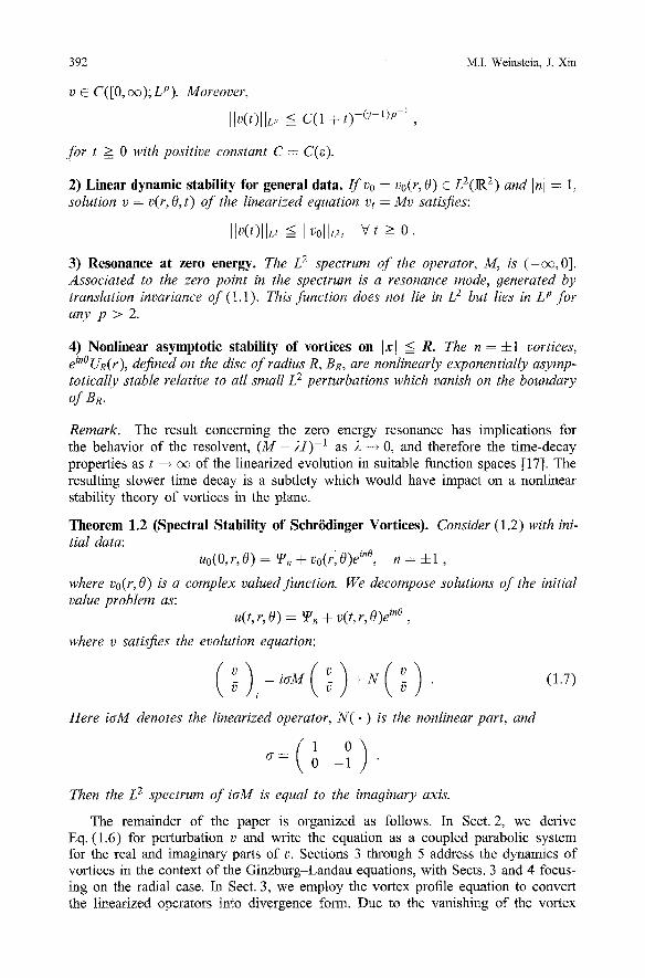
v E C([0, oo);LP). Moreover,

Ilv(t)llL~ = C(1 + t) -(~ l ) P - I ,

for t > 0 with positive constant C = C(e).

2) Linear dynamic stability for general data. Ifvo = vo(r, O) C L2(~-~ 2) and Inj = 1,

solution v = v(r, O, t) of the linearized equation vt = My satisfies:

Itv(t)llL2 ~ IIv011L2, v t ~ 0.

3) Resonance at zero energy. The L 2 spectrum of the operator, M, is ( - ~ , 0]. Associated to the zero point in the spectrum is a resonance mode, generated by translation invariance of (1.1). This function does not lie in L 2 but ties in L p for any p > 2.

4) Nonlinear asymptotic stability of vortices on Ix[ ~ R. The n = • vortices, e in~ UR(r), defined on the disc of radius R, BR, are nonlinearly exponentially asymptotically stable relative to all small L 2 perturbations which vanish on the boundary of BR.

Remark. The result concerning the zero energy resonance has implications for the behavior of the resolvent, (M - 2 / ) - I as 2 -~ 0, and therefore the time-decay properties as t ---+ oc of the linearized evolution in suitable function spaces [17]. The resulting slower time decay is a subtlety which would have impact on a nonlinear stability theory of vortices in the plane.

Theorem 1.2 (Spectral Stability of Schr6dinger Vortices). Consider (1.2)with initial data:

uo(O,r,O) = 7in + vo(ri O)e inO, n = • ,

where vo(r, O) is a complex valued function. We decompose solutions of the initial value problem as:

u(t, r, O) = 7tn + v(t, r, O)e in~ ,

where v satisfies the evolution equation:

( v ) t = i a M ( V ) + N ( V ) . (1.7)

Here iaM denotes the linearized operator, N( �9 ) is the nonlinear part, and

(10) a = 0 - 1 "

Then the L z spectrum of iaM is equal to the imaginary axis.

The remainder of the paper is organized as follows. In Sect. 2, we derive Eq. (1.6) for perturbation v and write the equation as a coupled parabolic system for the real and imaginary parts o f v. Sections 3 through 5 address the dynamics of vortices in the context of the Ginzburg-Landau equations, with Sects. 3 and 4 focus- ing on the radial case. In Sect. 3, we employ the vortex profile equation to convert the linearized operators into divergence form. Due to the vanishing of the vortex

Dynamic Stability of Ginzburg-Landan and Nonlinear Schr6dinger Equations 393

profile at r = 0, the parabolic operator of divergence form is degenerate at zero. We adapt the classical Nash-Aronson estimates using cutoff functions to obtain a pointwise Gaussian upper bound for the fundamental solutions. In Sect. 4, we apply these results to get decay estimates for linear semigroup and then prove the nonlinear asymptotic stability of all n-vortex relative to radial perturbations. In Sect. 4, we use the variational characterization of principal eigenvalues, and the maximum principle to prove parts (2) and (3) of Theorem 1.1. We identify the possible growth modes of perturbations in n-vortex, Inl > 2. We also comment on how to adapt our method here to show nonlinear asymptotic stability of one vortices on the finite disc domain with given Dirichlet data as treated in [19] and [22]; see Theorem 5.2. In Sect. 5, we prove Theorem 1.2 using results in Sect. 4, as well as the Hamiltonian structure of (1.7).

2. Preliminary Analysis

We consider the Ginzburg-Landau equation:

ut = Au + (1 - ]ul2)u, x E ]R 2,

ult-o = uo (x ) , (2.1)

where u : IR~ • ]R 2 ----+ ]R 2, and A is the two dimensional Laplacian. It is known that (2.1) admits vortex solutions of the form:

~Pn = Un(r) einO, n = =kl,-4-2,.... (2.2)

The basic properties of U , ( r ) are [24]:

1) U~(r) is the unique solution to the ODE problem:

! n2 grr+ gr-~g+(1-g2)g=o,

U(O) = O, U ' ( r ) > O, U(§ = 1. (2.3)

2) U~(r) has asymptotic behavior:

Un(r) ~ ar n (1

where a is a positive constant, and

r2 ) 4 n ~ 4 ' a s r - - + 0 , (2.4)

n 2

U , ( r ) ~ 1 2r2, as r ---+ oc . (2.5)

We are interested in studying problem (2.1) with initial data:

Uo(X) = (Un(r) + vo(r, O))e i'O , (2.6)

where (r, 0) is the polar coordinate of IR 2, and vo(r, O) is a small perturbation in LP(]R2), with p > 1 to be specified. We remark that writing the perturbation as in (2.6) is technically convenient for our later analysis and has no loss of generality. To examine the evolution of perturbation vo(r, O)e i'~ we write u as

u(t, r, O) = ( U , ( r ) + v(t, r, O))e in~ . (2.7)


Substituting (2.7) into (2.1) and using Eq. (2.2), we derive the following equation for v:

2ni n 2 vt = Av + 7 v o - 7 ~ v - U 2 v - U 2 g + ( 1 - U2)v

- g ~ l v l 2 - (2U~Re{v} + Ivl2)v, (2.8)

where My is the linear part and N ( v ) is the nonlinear part. Later, we will write v into its real and imaginary parts (v = c~ + iri), and will also use M to denote the resulting linear operator. Some details in deriving (2.8) are:

(veinO)t = A(Un(r)e inO) + ~d(ve inO) + (l - ]Un +/)12)(Un ~- v ) e inO ,

vt = - ( 1 - U2)U. + e-i"OA(ve i"~ + (1 - lUg, + vl2)(U. + v ) ,

where we have used 2ni n 2

e-i~~176 = Av + -~-vo - rTV,

and 1

VO = - - ( - sin O, cos 0 ) . r

I f we express v in terms of its real and imaginary parts, v = c~ + ifi, Eq. (2.8) can be rewritten as the system:

2n - 7 at = Ar - 7~rio + + 1 - 3U, 2 c~ - Un(c~ 2 + 1/2) _ 2U~c~2 _ (~2 + r iz)e ,

2n - 7 ri, = Ari + 7 ~ o + + 1 - U~ ri - 2Un~ri - (~2 + ri2)ri, (2.9)

with initial data: (~0(r, 0), rio(r, 0)).

R e m a r k 2.I . In the case of the dynamics of Schr6dinger vortices, then we replace the left-hand side of (2.1) with -Jut . Subsequently in (2.9), the left-hand side vector (c~t, ri,)r is replaced by -Jo(o'gt, fit) r, where d0 is the unit symplectic matrix ( o o l ) .

We shall first consider the radial case, i.e., c~0 = C~o(r), rio = rio(r). For functions = c@,t) ,and ri = ri(r,t), the system (2.9) reduces to:

O~ t ~- ~ I n ) o ; _ Un(O~2 @ f12) _ 2Uno:2 _ (g2 q_ r i2 )o ,

fit = 5~(n) fi - 2 U ~ r i - (0{ 2 -}- ri2)ri (2.10) 2

(n2 ) s = A + - 7 + 1 - 3 U 2 ( r )

- + - 7 + 1 - U (r)

where

(2.11)

The operators have domain of definition @ = {u E H2(IR 2) : r - 2 u C L2(IR2)}. We will estimate the semigroups generated by these two operators, and establish decay o f solutions for system (2.10) in the coming two sections. Our results will hold for any n, so for ease of presentation we only consider n = 1. We will replace Un by U, and abbreviate the operators in (2.11) and (2.12) into ~ai, i = 1,2.

(2.12)

Dynamic Stability of Ginzburg-Landau and Nonlinear Schr6dinger Equations 395

3. Gaussian Upper Bound for the Semigrnnp e ~21

In this section, we derive the Gaussian upper bound for the fundamental solution of the parabolic equation:

ut = s (3.1)

Equation (3.1) is not in divergence form. The key idea is to make use of the vortex profile equation (2.3) to convert it into one. Let us verify the identity:

(u-l~C~'zU)q = U - 2 V �9 ( U 2 ~ 7 q ) , (3.2)

for any smooth function q = q(r, 0). We compute:

A ( g q ) = ( A U ) q + UAq + 2 V U . Vq

= _(l_U2 l) - 7 ~ U q + U A q + 2 V U . V q ,

SO

A + 1 - U 2 1 ) - 7g (Uq) = ~*~

= U -I �9 (U2Aq + 2 U V U . Vq) = U - I v �9 ( U Z V q ) ,

which is just (3.2). The semigroup e se2t is positivity preserving by parabolic maximum principle or by the Feynman-Kac formula [32]. I f U were not zero at r = 0, then in view of (3.2), we could directly apply the results of Nash [23], Aronson [1], Osada [27] and others (see [8, 13,26] and references therein) to conclude that U-15~2U or 5('2 itself has pointwise upper and lower Gaussian bounds for their solution kernels. However, the fact that U(0) = 0 makes the problem degenerate and prevents us from doing so. Actually there is no Gaussian lower bound for ~a2. This is easily seen; because for r ~ 0, $ 2 ~-" (A + 1 - ~ ) which implies exponential decay o f e ~eit near r = 0. To establish the Gaussian upper bound, we will introduce a smooth cutoff function ~/ compactly supported in a ball centered

1 at zero. Outside this ball we use identity (3.2) and inside the ball we use the r2 term of s to help us overcome the degeneracy caused by U(0) = 0. A careful construction of ~/is necessary to piece the two parts together and achieve the Gaussian upper bound for the solution kernel of ~ 2 . We find it convenient to proceed along the line of proofs in Osada [27], who in turn followed the original ideas of Nash [23], Aronson [1], as well as Aronson and Serrin [2].

The properties of the function ~/ are summarized in:

L e m m a 3.1. There exists a C2([O, oe)) function ~1 = *l(r), r > O, such that:

1) r/(r) =- 1, / f r E [0,r0] , where r0 c (0, 1); 2) ,l(r) =_ O, i f r > rl, where rl c (ro, 1), and r 1 > 0 i f r E [0,rl); 3) 0 < 17(r ) < 1, rlr(r) <= O, for all r >= 0; 4) f o r any r ~ supp{r/},

2 41tbl 2 At1/ 2 - 2 U 2 - ~ - § - q =< - 1 ,

and 1 - f 2 1 lOIr/~l~ Arq

- - 7 -}- y/2 q- t/ ~ 0 ,

Proof See appendix. Let p = p(t -s ,x ,y) be the fundamental solution of (3.1), which satisfies the

semigroup property:

p( t - s , x , y )=fp ( t - z , x , z )p ( z - s , z , y )dz , s <z < t. (3.3)

We then have:

Proposition 3.1. only on the vortex profile U, such that:

f p2(t-s,x,y)dy < R 2

f p2(t - s,x,y)dx < R 2

p(t - s,x, y) <

For any s < t, x, y ~ ~R 2, there is a positive constant C, depending

C ( t - s ) -1 , ( 3 . 4 )

C ( t - s ) -1 , (3 .5 )

C ( t - s ) - 1 . (3 .6 )

Proof Note that (3.4) and (3.5) are similar, and (3.6) follows from (3.4) and (3.5) by the semigroup property. So we focus on the estimate (3.4). Next observe that we can, without loss of generality, set s = 0, and x = 0. It follows from (3.2) that:

qs = qU(U-I s q) = qUU-2V . (U2V(U-l q))

= U - l q V . ( U a V ( U - l q ) ) . (3.7)

Let E(t) = fp2. (r/2 + (1 - r/)Z)dy.

With the notation, f = fR2 dy, we have:

Et = f 2ppt(t/2 + (1 - t/)2)dy = f 2ps + (1 - t/)2)dy

= f 2(P~IZ)(Ap+ ( 1 - u Z - ~ ) P)

+f 2p(1-q)Z(Ap+ ( 1 - u Z - ~ ) P)

=_I+II.

Concerning/ , our strategy is to use the dominance of - r -2 for small r.

I = - f 2 V ( p ~ 2 ) . V p + 2 f ( p ~ ) 2 ( l - U 2 - 7 51)

= - 2 f [ r /V(pr / )+ pr/Vr/]. Vp + 2fp2r/2 (1 - U 2 -7~1 )

= - 2 f V(pr/) �9 (t /Vp + pVr/) + 2 f pV(p t / ) �9 Vr/

-2 f r lVr l 'PVP+2fp2r l2 (1 -U2-71 )

(3.8)

(3.9)

(3.1o)

(3.11)

= - 2 f [V(p~/)[ 2 + 2 f pV(prl). Vrl

§ f V(rlVrl)pz + 2 f p2rl2 ( 1 - U2 - ~ ) (3.12)

<-f]V(pt l )[ i+f[[Vt l lgp2+V(t lVt l )p2+2~12p2Ql-g2-~)]

( 2 21V~12 ~) = - f [V(p~/)[ 2 + fparl= 2 - 2U 2 - ~ + ~ + . (3.13)

By the Nash inequality [23]: Ilull 4 __< colllu[12llVul[ 2,

(f(pq)2)2 > ~ (f(pr /)2)2 f [V(pq)[ 2 > co ( f p ~ ) 2 = ~o ( - ~ - co(fp2~12) 2 , (3.14)

where co is a universal constant. Inequality (3.14) implies from (3.13) that:

/ I < - c o ( f p 2 r l 2 ) 2 4- fp2tl2 ~2 - 2 U 2 - -

Now using (3.7), we have:

II = 2 f ( 1 - t l ) 2 U - I 1 2 7 V , ( U 2 V ( U l p ) )

- 2 f U2V(U-lp). V((1 - ~ / )2U- lp )

2 -- r/~-- + . (3.15)

z -21" U2((1 - r/)V((1 - ~l)U-~p) + ( l - r/)U I p V ( l - r /)) . V(U-~p)

- 2 f U2[V((1 - ,I)U lp)( (1 - r / ) V ( U - l p ) + U - l p V ( 1 - r/))

-U-lpV(1 - tl). V((1 - rl)U-Ip) + (1 - r / ) U - l p V ( 1 - t/)- V ( U - l p ) ]

= - 2 f U2[IV((1 - r / ) U - l p ) [ 2 - ( U - ' p ) 2 [ V ( 1 - ~/)[2]

- 2 f U2[V((1 - t / ) U - l p ) l 2 + 2 f p e [ v q l 2

< -2c, f IV((1 - ~/)U-~p)I 2 + 2fp2jVrlr 2 , (3.16)

where here and below c~ > 0 denotes a constant depending on r/. Again, by Nash inequality, we have:

f IV((1 - rl)U-Zp)l 2 > on(f(1 - / ~ / ) 2 p 2 ) 2 (3.17)

Inequalities (3.17) and (3.16) yield:

II <= - c , ( f ( 1 - ?/)2p2)2 ~_ 2fp21Vt/[2. (3.18)

Combining (3.15) and (3.18), we get:

Et = I + II

< -min(c0 , c~)((fp2q2) 2 + ( f ( 1 - ~)2p2)2)

2 4 IVt/12 + f P2t12 (2 - 2U2 - ~ + ~ - - + ~ )

1 < - - min(co, c~)(fp2(q 2 + (1 - ~/)2))2 = 2

( 2 4 ' V t / ' 2 - ~ ) +fpa~2 2 - 2U 2 ~-~ + t / ~ + ,

o r

1 ( 2 E t <= -~min(co , cq)E 2 + fp2q2 2 - - 2 U 2 - ~ § - -

By Lemma 3.1, we then have:

which implies:

o r

4lvql2 ~ ) t/2 + . (3.19)

1 Et < - ~ min(c0, c n ) E 2 - fp2q2 , (3.20)

1 EI < - ~ rain(c0, c~ 7)E 2 , (3.21 )

E(t) < _C V t > 0 , (3.22) = t '

where C depends on ~/ and U. Inequality (3.4) follows. This completes the proof.

Proposition 3.2. Let r > O,(r be fixed. Let v(y) E Lz(IR 2) NL~176 2) such that v(y) = 0 if ]y - x] < r. Suppose that u(t, y) is a solution of the Cauchy problem of(Or - Y2 )u = 0 in (a, oo) x IR 2 with initial vahte u(a,y) = v(y). Then for any t, ~ < t < a + r 2, we have:

lu(t,x)l <= C(t - ~)-~ . exp{-Cr2/( t - ~))llvl12, (3.23)

with C a positive constant.

Proof Without loss of generality, we assume ( a , x ) = (0,0). For 0 < s < t, define:

h(s, y) = - C t [y12/(2t - s) , (3.24)

for some C1 > 0 to be chosen. Consider the equation

ut A u + ( 1 U2(r) ~ ) = - - u - ~ 2 u , (3.25)

and set m(r) = r/2 + (1 - r/) 2 .

Multiplying both sides of (3.25) by m(r)ue 2h, integrating over (0, ~) x IR 2, we have:

f fm(r)ue2~u, ds dy = f d s f m(r)ue2h(Au + (1 - U 2 - r - 2 ) u ) d y . (3.26) 0 R 2 0 R 2

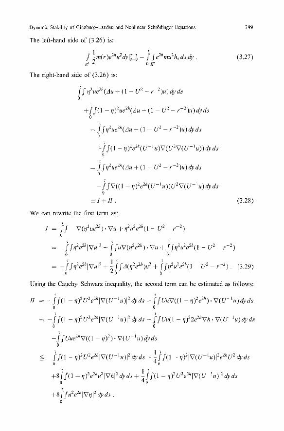
The left-hand side of (3.26) is:

f ~m(r)e2hu2dylS-~o- f fe2hmu2h, dsdy. (3.27) R 2 0 R 2

The right-hand side of (3.26) is:

~ff rl2ue2h(Au -+- (1 - U 2 - r - 2 ) u ) d y ds o

T

+ f f(1 - tl)2ueZh(Au + (1 - U 2 - r - Z ) u ) d y d s 0

= ff t l2ue2h(Au + (1 - U 2 - r - 2 ) u ) d y d s 0

+ f f(1 - ~ ) 2 e 2 h ( u - l b t ) V ( U 2 V ( U - l u ) ) dy ds o

T

= ff t l2ue2h(Au + (1 - U 2 - r - 2 ) u ) d y d s 0

- J ' f V ( ( 1 - r l ) 2 e 2 h ( U - l u ) ) U 2 V ( U - l u ) d y d s 0

_= I + / / . (3.28)

We can rewrite the first term as:

[ = f f - - V ( t / 2 u e 2 h ) �9 V u + q 2 u 2 e 2 h ( 1 - - U 2 - r -2) o

"g ~ "C

2 2h 2 2 2h 2 2 2h - f f u V ( ~ e ) V u + �9 ff~ u e (1 V 2 = - f f ~ l e IV.I _~-2 ) o o o

T 2 2h 2 1T i f 2 2 h 2 2 2h f f t l u e ( 1 - U 2 A(~ e )u + - r -a) (3.29) = -ff e Iv.P

o o

U s i n g t h e C a u c h y - S c h w a r z i n e q u a l i t y , t h e s e c o n d t e r m c a n b e e s t i m a t e d a s f o l l o w s :

II = - f f ( 1 - 1])2S2e2hlv(s- lu)12 dyds - f f UuV((1 - q ) 2 e 2 h ) - V ( U - l u ) d y d s 0 0 "C 7;

= - f f ( 1 - n)2uzs ~u)l 2 d y d s - f f u u ( 1 - t/)22e2hVh �9 V(U- 'u)dyds o o

T

_ f f Uue2hV((1 _ ~/)2). V ( U - l u ) dy ds o

< - f f ( l o - rl)ZU2e2hlV(U-~u)12 dyds+ ~ f f ( 1 - ~)21V(U lu)12e2hU 2 dyds

": 1 z

+ S f f ( 1 0 - - rl)2e2hu21Vhl2 dyds -l- ~ o f f ( 1 - r l )2g2e2hlv(g lu )12 dyds

+S f f u%2hlVrll 2 dy ds . o

400 M.I. Weinstem, J. Xin

2 f f(1 - ~)2u%2hlV(U-~u)l 2 dy ds

2 2h 2 +8f fe2hu2lVh[2 dyds + 8f fu e [Vq[ dyds. (3.30) o o

It follows, using the properties of ~I in Lemma 3.1, that

Z@II < f f [ ~ @ l O Vrl2+(1-U2-r-2)] ~-

+ f f (lVh[2tl 2 + 10[Vhl 2 + Ah)e2hu2dyds o

< ff(Ah + ll[Vhl2)e2hu2dyds. (3.31) 0

By (3.26),

m(r)e2hu2];-~ o < f f(mh, + lllVh[ 2 + Ah)u2e2hdyds o

=< f f (44C1(C1- ~4) ~s]Y[2 2t----s/4Cl ~ u2e2hdyds. (3.32 ) 0

Choose Ct = ~min{m(r)'r C IR+}. Then (3.32) implies, since v is supported where l yl > r, that

sup f e2hu2(s,y)dy <= C f m(r)e2hv2(y)dy. (3.33) sC[0,t] 4lylZ<<_t ly[>r

For (s, y) such that s ~ (0, t), 41Yl 2 < t, h(s, y) => - -~; for (s, y) such that s ~ (0, t), ly l > ~:

C1 r2 Clr 2 - 2 t - s 2t

Thus C 1 r 2 C 1 r 2

sup f u2(s,y)dy < Ce ---c- f v2(y)dy < Ce-=-llvll~, sC[O,t] 4lyl2_<_t [yl > r

and so t

f f u2(s,y)dy ~ Cte-@ll~lh~. 0 41y12 <t

By the local parabolic estimate (see Proposition 3.4 below):

u(t,O) <-_ Ct -~ f u2dyds , 4lyl2_-<t

for some C > 0. It follows from (3.34) and (3.35) that

(3.34)

(3.35)

(3.36) 1 r 2

u(t,o) ~ Ct-=e-C~vl]vlk2,

for t C (O, r2]. The proof is complete.

Dynamic Stability of Ginzburg Landau and Nonlinear Schr6dinger Equations 401

Theorem 3.1, Let p(t,s;x, y) be the fundamental solution of ut = s 2u. Then

0 s, x, y, where C1 and C2 are two positive constants depending only on U.

Proof. We follow the arguments of Aronson [1] or Osada [27], and include them here for the sake of completeness. First, if t - s > r 2, by Proposition 3.1:

Ix-A 2 p(t ,s;x ,y) < C ( t - s ) -1 __< C ( t - s ) - l e 4<,-,~ (3.38)

We now focus on the case t - s __< r 2. As in the proof of Proposition 3.1, the pointwise bound (3.37) is obtained using the semigroup property of p ( t - s,x,y), (3.3). We first break the integration region in (3.3) into the regions {z" Iz - x I > r} and { z ' l z - x [ < r}, and apply the Cauchy-Schwarz inequality to obtain

p(t - s;x, y) < J1 + J2 ,

J1 = f p2('c - s ; x , z ) d z p 2 ( t - z ; z , y ) d z Jz-x[ >_r Iz-xJ =r

and

J2 = p;(z - s;x,z)dz p2(t - ~; z, y)dz , Iz _<r I- ~ xl=r

where s < r < t. We now show that for t - s < r2:

f p 2 ( t - s ; x , y ) d y < C ( t - s ) - % if2 (3.39) py-xl >r

To this end, we consider:

u(s,x) = f p(s - a ; x , z ) p ( t - a ;y , z )dz , (3.40) Iz-yl>~

which is the solution of equation u~ = 2a2u, s > a with initial data:

u(a,x)=O, i f l x - y [ < r ; u ( a , x ) = p ( t - ~ r ; y , x ) , i f I x - y [ > r . (3.41)

By Proposition 3.1, u(~r,x) E L z NL~176 and by Proposition 3.2:

1 Cr 2

u(t,y)= f p2(t-~r;y,z)dz <-_ C(t-~)-~e-~]lu(~,z)ll2, Iz-yl>r

which implies (3.39) by Proposition 3.1. Similarly,

Cr 2

f p2(t-- a;y,z)dy < C ( t - a ) - l e (,-~) (3.42) I z - y l > r

where

Now set r = Ix-yl ~ = (s+t) and assume t - s < r21 Using (3.39) and Proposition 2 , - T - = 3.1, we get

s ) - l e - C ~ Ix - yl } J1 < C ( t - < C ( t - s ) -~ exp [ - c t - s - " (3.43)

For Ja, we see that tz - x I < r - Ix-yL implies Iz - y] > r. Hence we have 2 ---~

J2 <= f p2(s - "c;x,z)dz f p2(t - "c;z, y )d z Iz-xl<r Iz-xl<=r

<= f p2(s -- "c;x,z)dz f p2(t - "c,z, y ) d z Lz-yl>r Iz-yl>r

by (3.42) and Proposition 3.1 C l x - y l 2

C(t - s ) - l e ,-, . (3.44)

Thus (3.37) holds if t - s < r 2. This completes the proof. Finally, we outline the proof of the local parabolic estimate:

Proposition 3.3. Let u be a solution to ut = ~'2u and

Q = Q(y, a, t) = {x E IR 2 Ix - yl 2 < (t - a)/4} x 0r, t ) .

Then there exists a constant C independent o f u, ~r, t and y such that

1

lu(t,y)l < c ( t - o ' ) - 1 u 2 . (3.45)

Proo f In view of (3.2), and that by comparison &a2 is below A near r = 0, it is easy to check that the fundamental inequalities o f Aronson and Serrin [2] (or Proposition 2.2 of Osada [27]) hold for operator 2,f2. The rest follows from [2] on local properties of solutions of parabolic equations.

4. Nonlinear Asymptotic Stability in the Radial Case

In this section, we prove that any n-vortex solution is asymptotically stable under small radial perturbations (part (1) o f Theorem 1.1). We will proceed with n = 1; the proof in the general case is the same except for minor modifications. Let us consider the parabolic system:

gt = ='~1 c~ - - U ( 0~2 -~- f 2 ) _ 2Uo~2 __ (0{2 7- f l 2 ) g , (4.1)

Bit = •2fl - 2Uteri - (c~ 2 + f i 2 ) f , (4.2)

where 1 -- 3U2( r ) ) c~, ~c,('lc~ = Ac~ + -r-5 + 1 (4.3)

(1 ) ~<~2f = A f + - - ~ + l - U2(r) f t . (4.4)

Dynamic Stability of Ginzburg-Landau and Nonlinear Schrrdinger Equations 403

The initial data (c~0,fi0)E (LP(IR2)) 2, for some p E (1, oc) to be specified. When (c%fi0) is radially symmetric, system (4 .1) - (4 .2) governs the dynamics of radial perturbations of the one-vortex solution. We will establish a decay result for mild solutions of (4 .1) - (4 .2) in L p spaces without assuming radial symmetry.

We first note that the semigroups e tzei, i = 1, 2, are positivity preserving. Re- sults of the last section imply that e t~2 has a Gaussian upper bound, and so by a comparison argument, we have:

Proposition 4.1. The semigroup e ts satisfies:

Ile'Se2q:,[[p<Cll~ollp, v t > = o , V p c [ 1 , + o c ] , V ( p c L P ( ] R 2 ) , (4.5)

and [let~2~ollq <__ c t ( p - l _ q ~)lt~ollp ' v 1 __ 0 independent o f p.

The next step is to obtain an upper bound for e tLp~ . Following the proof of Proposition 3.1, inequality (3.20), and writing L*al = s176 - 2 U ( r ) 2, we find that

E(t ) = f r2( r /2 + (1 - r/)2), R2

where F is the fundamental inequality:

Et < = -- ~ c q E 2

1 2 <= - ~ c n E

solution of the equation ut = s satisfies the

- fF2t l 2 - 2fF2U(r)2012 + (1 - t/) 2)

-- fV2[r/2 q- 2U(r)2(r/2 q- (1 --/7)2)]. (4.7)

Since r / = 1 for r c [0, r0], we have on this interval that

/72 7- 2U(r)2(r/2 q- (1 - t/) 2) ~ t/2 = (t/2 -~ (1 - / 7 ) 2 ) .

On the other hand, r > r0, we have

2U(r)2(r/2 Jr- ( l - r/) 2) ~ 2g(ro)2(r] 2 + (1 - r])2) .

It follows that

1 2 Et <= - ~ c ~ E - min (1 ,2U(ro)Z) f F2(q 2 + (1 - r/) 2) -= - c o E 2 - c lE .

Integrating (4.8) from zero to t, and using E -+ +0% as t ~ 0 +, we get

e -C i t E( t ) < e l c o 1

= 1 -- e - c V '

which implies that

(4.8)

E(t ) < C t - l e -<t , (4.9)

for any t > 0, where C > 0 depends on e0 and Cl. It follows that Proposition 3.1 holds for F with (t - s ) le-<(t-s) replacing ( t - s) -1. We are ready to show

Proposition 4.2. The semi#roup e tzp~ satisfies:

]]et~[[p <-_ C , (4.10)

for C > 0 independent o f p c [1,+co];

Ilet ellI2 =< re c,,., (4.11)

and ]]etZf~cp]]q < Ct-(P-~-q-~)e-CZt(P ~-q ~)]]p][p, (4.12)

for any 1 0, that

Ilet ' ol[ =< Ct-*e-~ (4.13)

For any u o E L P A L ~176 1 O, et~Uoi > 0 by strong maximum principle. The comparison principle says that

t ~ l -t: 0:tz e u 0 ~ e t ~ Z u ,

for any t,x. It follows that

IIJ'uollp <= Ile' 'u+llp + Ile' 'Uo llp

<= [[e'~Zu~l[p + Ilet~2u+pI p

< 2C[luo]]p, (4.14)

for any p E [1,+oc]. Interpolating (4.13) and (4.14) gives (4.12). Finally if we replace F by the solution u of equation ut = 5r in the proof of Proposition 3.1, and drop the terms - f ]V(uq) ] 2 and - 2 f u Z ] v ( ( 1 - q)U- lu ) [ 2, we obtain without using the Nash inequality:

Et < - C l E ,

which gives the L 2 bound (4.11). The proof is complete.

Remark 4.1. The estimate (4.11) may be true for any p E [1,oo], however we will not pursue it here since (4.10) and (4.12) are sufficient for our stability proof.

Based on Proposition 4.1 and Proposition 4.2, we present

Theorem 4.1. Let us consider the system o f integral equations corresponding to (4.1)-(4.2):

t c~ = e t~f~ C~o - f e (t- ')~' [U(~ 2 +/~2) + 2Uc~a + ~(c~2 +/~2)], (4.15)

0

t B = et~2[lo - f e(t-~)ze2 [2Ue/? + (c~ 2 +/~2)/~], (4.16)

0

with initial data (c~0,fl0) C (L p ALq(IR2)) 2, where p c [3,6), q = y-~p, y c (1 + P,3). Then there exists ~ > 0 depending only on U, p, 7, such that i f

max([[(~o, flo) lip, II(~o,/~o)llq) =< ~, system (4.15)-(4.16) has unique mild solutions (~,/3) c C([0, +oo); (LP(R2))2). Moreover, we have the decay estimates:

]l~llp(t) < C(1 + t ) -(~-I>p-~ , (4.17)

}[~[[p(t) =< C ( l + t ) 2(])--1)p--1 , (4.18)

for all t > O, where C = C(e) > O. In particular, (4.17) and (4.18) imply the asymptotic stability of the vortex solution U(r)e +iO under small radial perturbations.

Analyzing with the same method the analogous parabolic system:

~t = ~.~n)(~ __ Un(~2 __ f12) __ 2Unc~2 __ (0~2 j r f 1 2 ) ~ , (4.19)

/~t = S(2n//~ 2Unc~/? - - (0~ 2 J r f l 2 ) f l , (4.20)

where

we obtain:

(n2 ) ~,P~n)c~ = Ax,yC~ + --~5 + 1 - 3UZ(r) c~, (4.21)

5(~n)fl = Ax, yfl + - ~ f + 1 - UZ(r) fl, (4.22)

Corollary 4.1. Any n-vortex solutions Un(r)e inO, n = zkl,• . . . . , are asymptotically stable with algebraic rates 9iven by (4.17) and (4.18) under small radial perturbations in L p n Lq(]R2).

Proof of Theorem 4.1. First we show that (4.15)-(4.16) has unique local solutions in C([O, T4t);(LP(R2))2). Letting (R1,R2) be the right-hand side of (4.15)-(4.16), we estimate:

t

IIR~il; _-< cll~ollp + c $ ( t - s)-~/~e-Cl;-'(t-S~l]3~2 + f i i ; /2ds 0

t § f t-2/pe-2Clp-l(t-s) I]~3 + fl3l]p/3 ds

0 t

_-< C[l~ollp + C f ( t - s ) - l / P e -czp-~( t S)(ll~zld2 + ]]fill2)ds 0

t +C f (t - s)-2/Pe-2c'p-~(t-s)(]lo~ll3p + []/~[[3p)ds,

0

so for t ~ [0, T], T > 0, we have

sup IIR~l lAt ) - l lR~l ip ,~ <= Cll~Ollp+Cr 1 ~(1[~1 21p,~ + ll/~tlp, o~)2 O<_t<T

1 - 2 3 3 +CT P ( [ [ ~ [ ] p , cx~ ~-[ [~[[p,~). (4.23)

Similarly,

t

IIR211p _-< cIIBollp + cfllc~llp/2(t-s) -~/pds 0

t t +C fl Ic~2fll Ip/3(t - s) -2/p ds ~- c fllfl3l[ p/3(t - s) -2/p a s ,

0 0

which gives

t

]IR2llp,~ < cIIB011p+Cll=llp,~'l lPllp,~ sup f(t-s)-l/Pds tE[0,T] 0

t

+cI I~I ~ Ip,~'ll/~ll~,o~ sup f(t-s)-2/Pds tC[O,T] 0

l

+cII/~ll~,oo sup f ( t - s ) - 2 / P d s tE[0,T] 0

1 1

1 2 1 2 + C T -~1 c~ 2 3 �9 ]Iflllp,~ (4.24) I tlp,~ liflllp,~ + CT -7

It fol lows from ( 4 . 2 3 ) - ( 4 . 2 4 ) that (R],R2) is a bounded map from C([0, T]; (LP(R2)) 2) into itself; moreover, i f T < 6 = g)(II(c~o, flo)IIp), then there is a unique solution (c~,fi) c C([0, T]; (LP(R2)) 2) by the contraction mapping principle. Such a solution can be continued to any t < T*, for some T* < + o c .

Next we proceed to derive the estimate of I1(~, fi)l ]p(t), independent o f T, where t E [0, T], T > 3. Let us define the norms:

I l l=lllp ~ sup ( l + t ) " l l = l l ~ ( t ) , tE[0,T]

I l lPIII , , - ~up (~ + t )b l l / ~ l l , , ( t ) , rE[o, T]

(4 .25)

where T E (0, T * ) and a > 0, b > 0, to be chosen. It fol lows from (4.15) that

Ill<nip --< sup (l+t)alle'Sl~01ip tE[0, T]

t § sup (1 -+- t)"flle('-~)~eI(U(c~ 2 +/~2) q_ 2Uo~2 q_ ( g 2 __ fl2)~)llp

tE [o, T] 0

/ max / sup (i + )alle' ollp, sup (i +,)~

k, tE[o,~] tE[&T] / t

+ sup (1 § t )a f ( t - s)-l/Pe-C'P-'(t-S)l]3c~2 + ~211p/zds tE[0,T] 0

t

+ sup (1 + t )a f ( t -- S) 2/Pe-2elp-~(t-s)l]~3 + fl20:]lp/3ds t6[0, T] 0

Dynamic Stability of Ginzburg-Landau and Nonlinear Schr6dinger Equations

__< max(C(1 +~)~ sup (t-le-Cit) (q-I p-l)(1 +t)a[l~oIIq) tC[~,r]

407

t + sup (1 + t ) ~ f ( ( t - s ) - l e - c ~ ( t - s ) ) - l / P ( ( 1 + S ) - 2 a l l l ~ l l l 2

tE[0,T] 0

+(1 + s)-2bl[[fll[[2)ds

t +(1 + t )a f ( ( t -- s) l e -CI ( t - s ) ) 2/p(1 + s)-3~lllcc21[13ds

0

+(1 + t ) ~ f ( ( t - s)-le-C~(t-s))-2/p(1 + s)-2a-~l l lBZlr l 2 �9 I[l~lllp)dx 0

~: C(q,p,a)(ll~ollLpc~L~ + [ll~l[l~ + Ill'liP 2 + IIr~lll~ + Illfl[IF 2. IIt~lllp), (4.26)

under the condition

The integral tel-m

a < 2b . (4.27)

t sup (1 + t ) ~ f ( t - s) 1/pe-c~P-~(t-s)(1 + S) -2b ds

tc[o, T] 0

appearing in (4.26) is uniformly bounded in T under (4.27). Indeed,

t sup (1 + t)a f ( t - s)-l/pe-C~P-Z(t-s)(1 + s) -2b ds

tE[0,6] 0

t < (1 + cS)af(t - s ) - l / P d s = C(p ,a) t 1-2/p <= C(p,a)c51--2/p . (4.28)

0

On the other hand, for t E (6, T], we have

t--O t -6 f ( t -- s ) - l / P e - C l P - ' ( t - s ) ( 1 + S) -2b ds < C(p) f e-ClP-~( t -s ) (1 + S) -2b ds 0 0

< C(p,b)(1 + t) -2b , (4.29)

and

t t f (t -- s) -1/p e-CtP-l(t-s)(1 + S) -2b ds <= (1 + t - 6) -2b f (t - s) -1/p ds

t -6 t 6

-< (1 § t - c5) 2b(1 -- l /p)-l(~ I-1/p.

(4.30)

The other integral terms in (4.26) are analogous. Combining (4.28), (4.29), and (4.30), we arrive at (4.26). We obtain from (4.16) that

( ) llI/~lll~ ~ max C sup (l+t)~llflollp, sup (1-I-t)bct - ( q - ' - p ')}lflo}}q \ t~[o,,~] t~[6,r] /

t § sup (1 § t)b f ( t - s) -('P-~)p 'l}~fillp/~ds

t~[O, T] 0

t + C sup (1 § t)b f ( t - s)-2p-'(ll~213llp/3 § IlBgllp/3)ds.

tE[O,T] 0 (4.31)

We choose

and note that

q-a = b + p-1 , (4.32)

Ilc~Hllp/~ ~ (fI~IP/~IHIP/7) 7/p = < (fI~[P/(?-I))(~-1)/P(fI/3IP)1/P,

= I1~11~/(,-,)" IIHII~. (4.33)

Now (4.31) gives

t IIINllp ~ c l l ~ o l l ~ , ~ q + C s~p (1 +t)bf(t-s)-(~'-l)P-'llallp/(~_~).llflllpds

tC[o,r] 0

t § s~p (~ + t ) ~ f ( t - s ) -Zp- ' ( l l~ l l%. II/~ll~ + IINl3)ds.

t6[0,r] o (4.34)

Then if

by (4.15) again

q-1 > (7-- 1)P -1 , (4.35)

II~lIp/(~-l)(t) ~ Ct-(q-l-@-l)P-1)e-Cat(q-t-(7 1)p-')ll~olL q

t + f [leCt-s)~*(g(~2 + H 2) + 2Uo~ 2 § (0{ 2 § flR)~llp/(,-l)

0

< Ct-(q-~-(7-I)p-~)e-ctt(q-l-@-l)p-')l]O~OI]q

t § -- s ) - (2p t - (Y-1)P- ' )g -el(t-s)(2p-I - ( ' / - I )P - I ) [ 13c~ 2 + f121 IF/2

0

t § f (t - s ) - (3P- ' - (7 -1 )P- ' ) e -cl(t-s)(3p-l-(7-1)p ')1 [~3 § ~f1211p/3

0

<= Ct-(q ~-(~-l)p-')e-C~t(q-~ (~-l)p ')l[~ol[q

t

0

t 4-cf(( t -- s)-le -cl(t s)) 3p- l - (7-1)p i(11~113 + I1~11~" I1#11~)

0

Ct (q-l (7_l)p-,)e_C,t(q i (v_l)p-l)}l~Ollq + I (4.36)

Thus

sup (1 +t)2bI < c(11i~111~+/11#1112+111~i113+ II#lll~.lll~l/Ip), (4.37) tc[o,r]

where we have used the integrals

t f ( ( t - s ) le-C'(t-s))(2P-'-(7 l)p l ) ( ( l + s ) 2 a + ( l + s ) - 2 b ) 0

< C(1 + t) 2b, (4.38)

t f ((t - s ) - l e - c i ( t - s ) ) (3p 1-(~-1)P-1)((1 @ s ) -3a Jr- (1 + s) -2b-a) 0

< C(1 -- t) -2b , (4.39)

where C = C(a, b, p, 7) under the condition

0 < ( 3 - ~ ) p - 1 < 1, 0 < ( 4 - 7 ) p -1 < 1. (4.40)

Combining (4.34), (4.36), and (4.37), we get

fll#lllp _-< CIl#ollL,mLq + Cl[~ollq" IFI#III~ sup (1 + t ) b tc[o,r]

t x f(t - s) -0/-1)p-1C(s-le c l s ) ( q - l - ( 7 - 1 ) P - 1 ) d s

0

t +C sup (1 +t)b f ( t - s ) -(~-I)p 1(1 +s)-3bds

tr T] 0

t +C/ll~lrl~. III#IFIp sup (1 H-t)bf(t- s)-2P-1(1 +S)-2a-bds

tE[0,TI 0 t

+t i l l # I l l 3 sup (1 +t)bf( t -s)-epl(1 +s)-3bds, (4.41) tC[0,T] 0

where

0 = C(lll~lll~ -II1#111~ + IJl~rll~ § II1#111~. I[ l~l l [p)l l l#l l t~ �9

We optimize the decay rate by choosing

a = 2b, (4.42)

b = (7 1)p -1 , (4.43)

1 < ( 7 - 1)P -1 § 2b. (4.44)

It follows from (4.43) and (4.44) that

7 > l + p / 3 , 3b > 1, (4.45)

which implies that 2a + b = 5b > 1. Now (4.40) requires that 7 < 3. Since p __> 3, (4.45) says that 7 > 2 and 3 _-< p < 6. Thus given any p E[3 ,6 ) , we pick 7 E (1 + p/3 ,3) , (a,b) according to (4.42) and (4.43), q-1 = b + p-1 = yp-1. Then (4.35), (4.40) and (4.44) hold. It follows from (4.26) and (4.41) that

IPl( ,t)lllp =< CIl( o, to)[IL nLq + f(Ll/ lllp, Illtil[Ip), (4.46)

where f = f (x , y) is a fourth degree polynomial containing no linear terms. Thus if II(~0, t0)llL~Lq is sufficiently small, [ll(~,ti)lllp remains bounded for all time. The proof is complete.

5. Linear Stability in the Nonradial Case

In this section, we consider the evolution of general (nonradial) perturbations of vortex solutions, and prove part (2) of Theorem 1.1. We will see that, in contrast to the Inl = 1 vortices, there is a potential for destabilizing In[ > 1 vortices due to nonradial effects. This is in agreement with J. Neu's [24] numerical observations of the instability of higher In I-vortices, in particular the splitting of a n-vortex (Inl > 2) into n individual one-vortices under suitable perturbations.

The system governing the perturbation v = ct + i t of an n-vortex solution U~e in~ is

at = 5F~n)~ 2n -- 7 f i 0 -- Un(O~ 2 -1- fi 2) - 2Uno; 2 - - (0( 2 -{- fi2)O{ , (5.1)

tt (n) 2n = 5~2 t + 7T~o - 2U~c~t - (~2 + t z ) t , (5.2)

where (n2 ) Y{")ct = A e + - 7 + 1 - 3Uff(r) c~, (5.3)

5~")fi = A t + - 7 + 1 - U2(r) t . (5.4)

Consider the linear part. In view of the 0 independence of the coefficients, we expand into Fourier series:

Then (ctm, t im) satisfies (n2 O:m, t = ArO: m + -- 7~

flm, t = Ar f lm -}- - - ~

O: = ~ O:m eimO , ( 5 . 5 ) mff Z

fl = ~ tim eimO . ( 5 . 6 ) mEZ

- - 1 - 3UZ(r)) O:m + ~(-m2o:m - 2inmflm),

+ l - U2(r)) flm § ~(2inmo:m m2flm), (5.7)

or in vector notation:

am am - 7 + 1 - 3gff( r ) 0 C~m / /2 *

tim ~ ~ r fir// ~- 0 -- -F @ 1 - U 2n ( r ) tim

1 ( - m a - 2 i n m ) ( C~m ) (5.8) + ~ 2inm -m 2 " tim '

where Ar is the two dimensional radial Laplacian. The operator formed by the first two terms on the right-hand side of (5.8) is the operator we have analyzed in the radial case. It is easy to show that this operator has continuous spectrum equal to ( - o c , 0] and the Nash-Aronson estimates in Sect. 3 imply that the L 2 spectrum equals ( - o c , 0]. The "rotational terms" r-2fio and r-2c~o produce the matrix:

--m 2 --2inm ) 2into --m 2 , (5.9)

whose determinant is equal to m2(m 2 - 4n2). Therefore, the matrix (5.9) has positive eigenvalue if

m+O, m 2 < 4n 2 , (5.10)

and the possibility of instability exists. As n increases, the number of potentially destabilizing modes increases.

In case In] = 1, only m = • could be a source of linear instabilities. While if m + + 1, then (5.9) is nonpositive, so by our results in the radial case, such (am, tim) would decay to zero with time in L p spaces. Let us consider n = 1 and m = 1, the other cases o f lnl = lml = 1 are treated identically.

Let us transform (5.8) into a real coefficient system by first writing it as:

( cq ) t = ( A r + l - U 2 ( r ) ) ( cq ) i l l fll (5.11)

2(1 +~5 i - 1 " fll + 0 0 " fll "

The matrix (1,) i - 1

has eigenvalues 0, - 2 , corresponding to eigenvectors @2( i , -1 ) r, 1 ti 1 ~r Let us

make the change of variables:

cq 1 i i

then

where

2 ( 0 0 ) _ U 2 ( 1 1 ) (5.14) = ( A r + l - g 2 ( r ) ) I d + ~ 5 0 - 2 1 1 "

The following property of the one-vortex profile U is very useful in analysis appearing later in this section:

Proposit ion 5.1. Let U = U(r) be the one vortex profile. Then

r 1U(r) > U~(r), V r > O.

Moreover, the self-adjoint operator

2f3 -- A~ + (1 - 3 U 2 ( r ) ) ,

defined on H2(IR 2) has spectrum o ' (~3 ) inside ( -oc , -ao ) , for some positive constant ao.

Proof. Recall that U(r) satisfies the equation:

g~r+ gr-Tg+(1-g2)g:o, g ( 0 ) -- 0, g ( + e c ) = 1, g~(r) > 0 , (5.15)

for any r > 0. Differentiate (5.15) to r and denote U~ by w to get:

1 2 2 w~r+-W~r ~ - s U + ( 1 - 3 U 2 ) w = O '

or 1

Wr,- + --Wr § (1 -- 3U2)w = (w - r -1U) . (5.16) r

Now letting V = r-lU, we have from (5.15) that

(rV)rr + r- l (rV)r -- r -1V + (1 - U2)U = O,

or r V r ~ + 2 V r + V r + r - l V - r - l V + ( 1 - U 2 ) U = 0 ~

or Vrr+3r 1 V r = r - l ( u 2 - 1 ) U < 0 , (5.17)

for any r > 0. We consider inequality (5.17) on r E [e, rl], where e << 1, rl >> 1. r 2

For r small, U(r) ~ ar(1 - -~ + O(r4)), for some constant a > 0. Thus V(r) is monotonely decreasing in r if r is small enough. With e sufficiently small, we see that V(r) has to go through a local minimum if V(r) increases with r at all. In other words, there exists an interval [r2,r3] strictly inside [e, rl] such that V has a minimum over [r2,r3]. However, inequality (5.17) and strong maximum principle imply that V(r) = const, for r C Jr1, r2], or U(r) = const, r. Therefore i f r ~ [r2, r3], Urr = O, r-lU~ - r-2U = (r-iU)~ = 0, but (1 - U2)U > 0, contradicting (5.15). We conclude that

V ' ( r ) = ( U ) < 0 , (5.18) F

or rUt <-_ U(r), for any r > 0. If V ' ( r 4 ) = 0, for some r4 > 0, then (5.17) says that V'(r4) < 0, contradicting (5.18). Thus we have strict inequality in (5.18), and rUt < U(r), for any r > 0.

Next we consider the spectrum of 2'3. By Weyl 's theorem on the essential spectrum, we have that O'ess(2" 3 ) = ( - - O O , - 2 ] . Moreover, 2"3 has a principal eigenvalue cq and corresponding ground state eigenfunction Ul == ul(r) > 0 in L2(IR z) such that

2"3//1 = 0-1/,/1 , (5.19)

or what is the same: AUl § ( l 3 U 2 ( r ) ) u l = o I H I , ( 5 . 2 0 )

for any (x, y ) C IR 2. By elliptic regularity ul is a smooth function. Similarly, we write (5.16) as:

+ (1 - 3U2(r))w = ~ ( w - r - l U ) < 0 . (5.21) Aw

Both Ul and w decay to zero as r --+ oc. Multiplying (5.20) by w, and integrating over IR 2, we get with integration by parts that:

f mAw + f ( 1 - 3U2)WUl = crl f UlW , R 2 R 2 R 2

whose left-hand side is fe2 ~ ( U r - - r 1U)ul < 0. Noticing that fR2 UlW > 0, we infer that ol < 0, and the proof of lemma is complete.

Proposition 5.2. The vector

~(ur + u~ - = (~0,a0) r - l U ( r ) , F - 1 U )

satisfies 2"(~0, b0) r = 0, for any r = (x 2 + y2) 1. However, (7o, 60) ~L2(IR 2) but is in LP(IR 2) for any p > 2.

Remark. A mode of this type is frequently called a resonant state. It is known to influence the decay rate of the linear evolution operator generated by it. See, for example, [ 17].

Proof. It follows from (5.14) that W = 7 + 6 satisfies:

4 6 . Wt = ArW + (1 - 3 u Z ) w - )5 (5.22)

The pair (W,~/) is the solution to the system:

Wt = ArW +(1 - 3 U 2 ) W - ~ 2 ( W - y ) ,

?, = Ary + (1 - U2) '~ - U2W. (5.23)

Differentiating Eq. (5.15) to r and letting W0 = Ur, we get:

A~Wo + (1 - 3u i )Wo + 2 ( r - l U - Ur) = 0 . (5.24) r ~

414

Denoting

v/0 u Wo u 7 o = ~ - + 2 - ~ , ~o-- 2 2 r '

we have from (5.24) and (5.25) that

M.I. Weinstein, J. Xin

(5.25)

4 4 A~Wo +(I- 3U2)Wo- ~5o = A~Wo +(i- 3U2)Wo- ~(Wo- yo) = O.

Now using (5.24) and (5.15), we verify:

(AT + (1 - g2))~o - g2Wo

= ~(Ar + ( 1 - U2)) (Wo +-~) - U2Wo

= ~[(3U2 -1)Wo + ~(Ur - r-I U)] + ~ Ar(r-I U)

@~(1- U2)(Wo@ U ) - U 2 W o

= r-2(Ur - r -1 U ) - - ~ ( r - l U r r - 2 r - 2 U r + 2r-3U + r-2Ur - r -3 U )

§ - U2)U

= r-2(Ur - r -1 U) + ~(r-IA~U + r 3U - 2r-2U~) + (2r)- l (1 - U2)U

= r - 2 ( U r - r - l U ) + r -3U+~(r U-2r-2U~)=O. (5.26)

u Wo ~ ) vanishes •. Apparently, (7o, C5o)~(L2(IR2))2; Thus (7o,6o) = ( 9 + 2r, 2 however, belongs to (LP(IR2)) 2 if p > 2. By Proposition 5.1, 6o < 0, and 7o > 0, for any r __> 0. The proof is complete.

Proposition 5.3. Consider the self-adjoint operator ~ defined on

= {(~,(~) E H 2 • H 2 : r-26 E La(]R2)} ,

Then the spectrum of S is equal to (-oc, 0].

Proof. By Weyl's essential spectrum theorem, aoss(~r ( - ec ,0 ] . So we only need to prove that there is no positive eigenvalue. Suppose that al > 0 is the principal (the largest) eigenvalue of ~ . By the variational characterization of the principal eigenvalue, we have:

or1 = sup Q(7, 6) , (5.27) (~,(~)CH 1 •

Dynamic Stability of Ginzburg-Landau and Nonlinear Scl-u6dinger Equations 415

where

Q(a,b) = - f ( 7 2 + 62) + f(1 - 2U2)(72 q- 62) - 2 f U2?a - 4 f r-262 . (5.28) R 2 R 2 R 2 R 2

Notice that the maximizer (7" ,6") of Q must have 6*(r) --~ 0 as r -+ 0 for Q to stay finite. (7*, 6*) is a classical solution for r > 0. It is not hard to obtain 6*(r) < O(r 2) by balancing terms in ( 2 ~ - 61)(7*,6*) = 0. In fact, it follows from the 6* equation that

Arc~* -- ~ 6 "I" E LP(]R2) , (5.29)

for any p E [2,00) due to ( 7 " , 6 " ) E H I ( I R 2) and Sobolev imdedding. We can regard (5.29) as the e 2i0 mode restriction of the two dimensional Laplacian. Hence, 6* E W2'P(IR 2), p > 2, and is imbedded into C 2+e, e E (0, 1). Now we conclude by Taylor expanding 6* at zero, r-26 * E L2(IR 2) with (5.28), and (5.29). Thus (7",c~*) C D(~('). Thanks to the term --2fR2 U276 and that fR2 ]Vf[ 2 ~ L2 ]vlfl l 2 for any f E HI(1R2), we have

Q(7",6") < Q(lT*l,-lO*r),

which implies that 7* and 6* have opposite signs. That is either 7* > 0, 8" < 0 or vice versa. We arrange 7* > 0. Now forming the inner product in LZ(]R 2) (denoted b y ( . , - ) 2 ) o f

(~(' -- 0-1)(7",6" ) = 0, (5.30)

with (70,60). Since o-1 > 0, (7" ,6") decays to zero exponentially fast as r --+ oo. This can be seen as follows. The asymptotic behavior of U at infinity (2.5) implies that (5.30) is a weakly coupled elliptic system for large r:

( ) [ ( ) Y* 1 + ~r 1 1 + A(r) 6* = 0, Ar 6" -- 1 1 ~- (71

where A(r) is a smooth 2 by 2 matrix in r, and [IAIIoo < 0(?'-2). The matrix

( 1+o- 1 1 ) 1 1 + 6 1

is positive definite and so can be diagonalized by a constant orthogonal matrix Q1. Let

(71,61)T : (7", 6*)T QT ,

then (71,61) satisfies

( 7 1 ) - E( /~1 0 ) I ( 71 ) : 0 (5.31) ar 61 0 22 +B(r ) 61 '

for 2i > 0, i = 1,2, and a matrix B = (bij), I[B[[~ _-< O(r-2). Letting q = 721 + ~ ,

416

we have from (5.31):

A~q =

>

>_

>

271ArTl+21V71]2+261Ar614-2]V61] 2

271ArTl+261Ar61


2y l (2171+bl l ( r )y l+b12(r )61)+261(2261+b21(r )y1+b22(r )61)

2 1 ~ + 2 2 6 ~ > min(21,22)q, (5.32)

if r is large enough depending on )~i, i = 1,2. Now it is easy to find a comparison function ~ = e -~r, # > 0 such that

(At - min(21,22))c~ = (#2 _ ix/r _ min()q, 22))e - ~ =< 0 .

By comparison principle of scalar elliptic operators, we infer that

q < Ce-~ ~ '

for some constant C if r is large enough. In other words, (7*, 6*) decays exponentially fast as r -+ oc.

Thus we can perform integration by parts to get from (5.30):

((y*, 6"), f (70 , 60))2 = al((7*, 6"), (70, 60))2, (5.33)

whose right-hand side is strictly positive, and left-hand side is zero, impossible. Hence no positive eigenvalue exists for ~qo, and cr(~q) is ( - o o , 0 ] . This completes the proof.

We are now ready to prove part (2) of Theorem 1.1.

Theorem 53 . Consider the linearization o f ( 5 . 1 ) - ( 5 . 2 ) f o r the plus or minus one vortex and let a + ifi E L2(]I~ 2) be the solutions to the linearized system:

~, = 2P~ 1~- ~Po,

2 ]~t = ~ l ) f l Jr- ~ 0 , (5.34)

with initial data (~o + ifio) c L2(IRa). Then

11(~,/~)ll2(t) _-< 11(~0,/~0)112, (5.35)

for any t > O, i e. the plus or minus one vortex is linearly dynamically stable in L 2 with respect to arbitrary (nonradial) L 2 perturbations. Moreover, the linearized operator in (5.34) denoted by M is self-adjoint and nonpositive.

Proo f By our earlier discussion, we decompose (~, fl) into the Fourier series:

~(t, r, O) = ~ ~j(t , r ) e ijO , jEz

fl(t, r, O) = ~ fij(t, r)e ij~ . jGZ

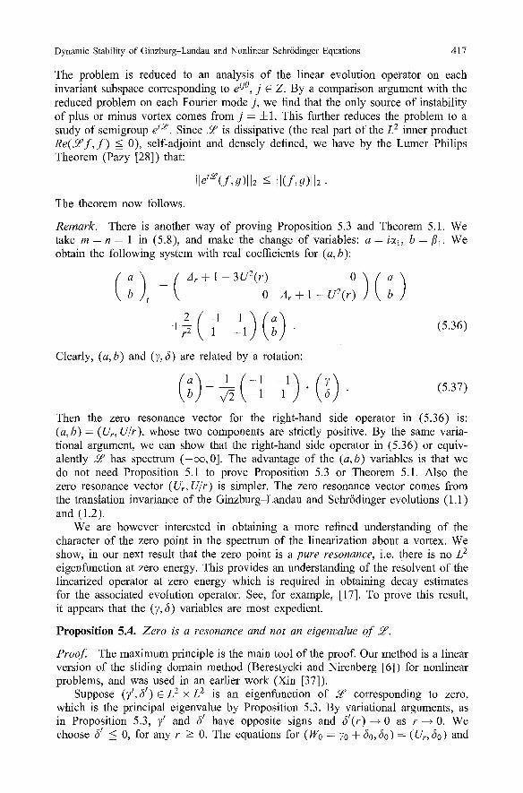
The problem is reduced to an analysis of the linear evolution operator on each invariant subspace corresponding to e i j~ j E Z. By a comparison argument with the reduced problem on each Fourier mode j, we find that the only source of instability of plus or minus vortex comes from j = 4-1. This further reduces the problem to a study of semigroup e t~e. Since ~ is dissipative (the real part of the L 2 inner product R e ( S f , f ) _-< 0), self-adjoint and densely defined, we have by the Lumer-Philips Theorem (Pazy [28]) that:

Plet~(f,g)ll2 < II ( f ,g ) l [2 .

The theorem now follows.

Remark. There is another way of proving Proposition 5.3 and Theorem 5.1. We take m = n -- l in (5.8), and make the change of variables: a = iel, b = ill. We obtain the following system with real coefficients for (a, b):

b t 0 Ar § 1 - U2(r) b

+ ~ ( 1 1 1 1 ) ( ; ) "

Clearly, (a,b) and (7, 3) are related by a rotation:

( ; ) = ~22 ( --11 1 1 ) " ( ~ ) "

(5.36)

(5.37)

Then the zero resonance vector for the right-hand side operator in (5.36) is: (a,b) = (U,., U/r), whose two components are strictly positive. By the same variational argument, we can show that the right-hand side operator in (5.36) or equiv- alently 5r has spectrum (-00,0]. The advantage of the (a,b) variables is that we do not need Proposition 5.1 to prove Proposition 5.3 or Theorem 5.1. Also the zero resonance vector (Ur, U/r) is simpler. The zero resonance vector comes from the translation invariance of the Ginzburg-Landau and Schr6dinger evolutions (1.1) and (1.2).

We are however interested in obtaining a more refined understanding of the character of the zero point in the spectrum of the linearization about a vortex. We show, in our next result that the zero point is a pure resonance, i.e. there is no L 2 eigenfunction at zero energy. This provides an understanding of the resolvent of the linearized operator at zero energy which is required in obtaining decay estimates for the associated evolution operator. See, for example, [17]. To prove this result, it appears that the (7, 3) variables are most expedient.

Proposition 5.4. Zero is a resonance and not an eigenvalue of 5~.

Proof. The maximum principle is the main tool of the proof. Our method is a linear version of the sliding domain method (Berestycki and Nirenberg [6]) for nonlinear problems, and was used in an earlier work (Xin [37]).

Suppose (7/, 3 ' )E L2• L 2 is an eigenfunction of 5~ corresponding to zero, which is the principal eigenvalue by Proposition 5.3. By variational arguments, as in Proposition 5.3, 7' and 3' have opposite signs and 6'(r)--+ 0 as r---+ 0. We choose ~/ < 0, for any r > 0. The equations for (W0 = 70 + ~0,60)= (Ur, 00) and

418

(W' = 7' + 6I, 6 ' ) are

ZIrW § (1 -- 3 U 2 ) W - 5 6 r2 = 0 ,

A ~ 6 + ( 1 - U 2 - 4 r - 2 ) 6 - U 2 W = 0 .


(5.38)

(5.39)

This implies, for 2 E ]R, that the functions

~gx -- ,~V/o - W',

satisfy:

64 -= 260 - 6 ~ ,

ArW2 § (1 - 3U2)W2 = ~262, (5.40)

Ar6~ + (1 - U 2 - 4r-2)6,~ = U2W)o . (5.41)

We first set 2 > 0. It follows from (5.40) that Wx ~ 0(r-26~.) due to 1 - 3U 2 ~ - 2 as r---+ ec. By (5.41) we have then: Ar6r ~ 0(r-26~) , which implies by direct integration that 6~,~ ~ 0(r-16~) , and 6X, r~ ~ O(r-262). Going back to (5.40), we see that W~.,~ ~ O(r-lWr and W,t,~ ~ O(r-2Wr or A~W~o is a higher order decay term than Wr So by (5.40), Wx ~ - 2 r - 2 6 r +h.o.t. Substituting this into (5.41) along with 1 - U 2 ~ r -2 + h.o.t., we obtain:

Ar62 + ( - - r -2 + h.o.t.)6~. = 0. (5.42)

Since 6' E L2(lR2), for any given )~ > 0, there is r0 -- ro(2) > 1 such that c~(r0) < 0. We can choose ro(2) large enough so that the above asymptotics become valid. By (5.42) and the fact that 6;.(r) -+ 0 as r ~ oc, we deduce from the maximum principle that 64 has neither a nonnegative maximum nor a nonpositive minimum for any r > r0. Therefore, 64 is negative for r > r0, and monotonically increases to zero as r ~ ec. In other words, 6' decays faster than 0(6o). In particular, there exists R0 such that:

6 ; ~ = 2 3 0 - ~ I < 0, i f r > R 0 , 2 > 1. (5,43)

By making Ro larger if necessary, we have U > 2/3 for r > Ro. We infer from (5.40) that

ArW2 + (1 - 3U2)W,~ ~ 0 , (5.44)

i f 2 > 1, r > Ro. For r E [0,R0], there exists A1 = AI(R0) => 1 such that i f 2 > A1, Wx(r) > 0 and 6,~(r) < 0, for any r E [0,R0]. Thus if 2 > A1, (5.44) and the maximum principle imply that W,t(r) > 0, any r => 0. Also fix < 0, V r C [0, oc). Similarly, there is A2 >= 1, such that i f )~ < -A2 , then Wx(r) < 0, 64 > 0, for any r ->_ 0. Define

= inf{2 E IRIlW~ -> 0 and fix < 0, V r E [0, oc )} .

Then # C ( -A2 , A1 ), Wu >= 0, 3~ =< 0, Vr E [0, oc]. Now suppose that # = 0, then 6u = -61 < 0. However, as initially observed, 6' < 0, and so 6' =- 0. By (5.38) and Proposition 5.1, we infer that W' ~ 0, or 7' ~ 0, contradicting the assumption that (7', ~ ') is an eigenfunction. We deduce that # > 0.

With 2 = # in (5.40) and (5.41), 6~ < 0, W~ > 0, strong maximum principle implies that either W~ > 0, ~ < 0, or Wa = c5~ - 0 for all r C [0, oo). The latter

implies #c50 - ~ and therefore 6o E L2(IR2), a contradiction. Now suppose that there is a sequence {2,}, 2~ C (0,#) , 2~ ~ #, as n --+ oo, such

that inf Wj..(r) < O, r > 0

for each 2~. Since W;o,,(r) --4 0 as r ~ oo, there is a sequence {in} such that

W,~.(rn) = inf W2o(r) < O. r>O

I f {r~} is unbounded, there is a subsequence, still denoted {rn}, with r~ ~ oc. I f n is large enough, r , > R0, then evaluating

4 6 r , ArW~,,(r.) + (1 - 3uZ)wz.(rn) = ~ ;~.( .)

at r = rn >> 1 yields

(A~W)~. + (1 - 3U2)Wx.)(rn) >= (1 - 3U2(rn))Wx.(rn) > O,

while 4

~(;~.~0(r~) - 6'(~n)) < 0 ,

because 2n --, # > 0, and 6' decays faster than 6o at infinity as we have showed above by (5.42). We have a contradiction.

Therefore, {r .} is a bounded sequence, and there exists a subsequence, which we also denote {r.}, along which we have r . -+ r * E [0, oc). It follows that

W~n(r.)--+ rYe(r*) __< 0 ,

as n -+ oc, contradicting Wu(r) > 0, any r > 0. This means that there is a number #1 E (0 ,# ) such that

inf Wr > O, VZ E (#1, #) , r>0

By minimali ty of #, we have

supf;o(r) > 0, V 2 E ( # I , # ) . r__>0

/ l ! Therefore, there exists a sequence {)o~}, 2. E ( /q ,# ) , 2. --+ #, as n - + oc, and a sequence of {r~} such that

(5.~.(r~.) = sup6z , ( r ) > 0 . r>0

I I f {rs is unbounded, then r n -+ oo, up to a subsequence still denoted the same. By Eq. (5.41) with 2 = 2n:

Arg)2. + (1 - U 2 - 4r-2)6~. = U2Wj,. > 0. (5.45)

! I f r n > > l , t h e n

1 - U Z ( r ~ ) = ( 1 - U ( r , ' , ) ) ( 1 + U(r;))

_ _

= (rl) e +h .o . t .

1 ) 2(rnt) 2 + h.o.t.

which shows that 1 2 t - - U ( r n ) - 4(rn/) -2 < 0 .

Evaluating (5.45) at r = rn >> 1 implies that the left-hand side is

< (1 - U 2 ( r ~ ) - 4(/n) 2)cSz,(r'n) < 0 ,

a contradiction. Finally, {r~} is bounded, and rn---' r * * E [0, e c ) along a subsequence still denoted the same. We have 5if(r**) => 0, contradicting our early conclusion that 5ff < 0. Thus all roads from the assumption of zero being an L 2 eigenvalue lead to a contradiction. We conclude that zero is not an eigenvalue but rather a pure resonance. The proof is complete.

Finally, we comment on how to adapt our method to treat stability of one vortices on the disc of radius R, denoted by BR. We will consider the plus one vortex to be specific. Let u = UR(r)e i~ be the plus one vortex solution on BR, and consider perturbation of the form v(t,r, O)e iO such that v(t,R, 0) = 0. Going through the same derivation as before, we see that (5.1-5.2) hold for the real and imaginary parts of v, with Un replaced by UR. We then decompose solutions into Fourier modes as in (5.5 5.6). For the radial part, or m -- 0, we follow the estimates in Proposition 3.1, however, they can be carried out directly on any solution v of the linear equation vt = 5f2v since we can use the Poincar6 inequality instead of the Nash inequality thanks to the zero Dirichlet boundary condition of perturbation v at r = R. The result is that v decays to zero exponentially fast in the L 2 norm with a rate depending on R. Thus we only need to verify that the linearized operator S ~ , which is just 2,~ in (5.14) with U replaced by /dR corresponding to the m = 1 mode, has strictly negative spectrum. Using this strict negativity of ~ , we can prove:

Theorem 5.2. Let Ue(r)e in~ be a Inl = 1 vortex on BR the disc o f radius R. Le t u = (UR(r) + v(t ,r,O))e i~ where v is the perturbation satisfying v ( t , R , O ) = 0 and v(O,r,O) E L2(BR). Then there exists constants 7 = 7 ( R ) > 0, and C = c(llv(O,r,O)ll2) > o, such that i f IIv(O,r,O)ll2 is small enough:

[[u(t,r,O) UR(r)ein~ <= Ce -Tt ,

holds f o r all t > O. In other words, the one vortices are nonlinearly asymptotically stable with exponential rate.

Proof. We show that the operator ~97~ has strictly negative spectrum. Since we are on a finite domain, ~ has only discrete eigenvalues in the spectrum except for - o c . Suppose that 21 > 0 is the leading eigenvalue corresponding to eigenvector (vb v2). By the variational principle, we can arrange so that vl => 0, v2 < 0. Forming the L 2 inner product of (70, c50) with

~-(PR(Vl, V2) T = ~vl(Vl, v2) T ,

integrating by parts, and using the zero boundary condition on (vl, v2), we get:

f (Vl,rY0 q- V2,r(~0) : "~q ((q/0, ~50), (Vl,/22))2 �9 (5.46) r=R

On the other hand, vl,r < 0, v2,r -> 0, at r = R, hence it follows that 2~ =< 0. So it is only possible that 2l = 0. Then the equation for Vl is

+ 1 - Z U 2 ( r ) > l - U (r) 2 = 0 ,

or (Ar -- 2 U 2 ( r ) ) v l = - V l q- g 2 ( r ) v 2 <= O,

which implies via the strong maximum principle that either vl = 0 or vl > 0 if r < R. Similarly, v2 satisfies the differential inequality:

(Ar -2U2(r ) ~ ) -- 122 = --/)2 -- U2( r )v l ~ 0 ,

and so either v2 = 0 or v2 < 0 for r < R. Since (vl,v2) is an eigenvector, one of its components is nonzero. Let us assume that Vl > 0 (or v2 < 0), r < R. Then by the Hopf lemma, Vl,r < 0 (or v2,,. > 0), at r = R. It follows that the left-hand side of (5.46) is strictly negative. We deduce a contradiction, and so 21 < 0. Since the spectrum is strictly negative, the linear evolution of the perturbation has to decay exponentially in time, and so is the nonlinear one as long as the initial perturbation is smali enough. The proof is complete.

6. Spectral Stability of the Schrtidinger One-Vortex

In this section, we show that the linearized operator for the Schr6dinger one-vortex, i a M - JM, has spectrum equal to the imaginary axis. Therefore the Schr6dinger one-vortex is spectrally stable. The perturbation v(t,x) = (~, fi)r to the Schr6dinger one-vortex solution satisfies:

g t = JM , (6.47)

ignoring the nonlinear terms of v. By Weyl ' s theorem, the continuous spectrum of JM is the entire imaginary axis, so we only need to show that there is no eigenvalue on the right half plane. Hamiltonian symmetry then ensures that there are no eigenvalues in the left half plane either.

Theorem 6.1. The operator irrM has L 2 spectrum equal to iN.

Proof The proof follows from a general result appearing in [29]. We present the argument in the current context. Suppose JM =_ iaM has an eigenvalue 2, Re{2} > 0, corresponding to the eigenfunction ~b. Then

JMO = )@, (6.48)

and so eJMtl/I = e2tl/l. (6.49)

Using skew symmetry of J and symmetry of M, we have for any u(t,x) satisfying ut = JMu:

z ( M u , u) = +

= ( MJMu, u ) + (Mu, JMu )

= (MJMu, u) 4- (MJ*Mu, u) = O, (6.50)

for any u C ~ ( M ) . It follows rather that

0 = d(MeXq~, e2tl/i )

which implies that

= de('~+X)t(MO, 0 ) ,

(MO, gt) = O.

Since - M is a nonnegative self-adjoint operator,

( - M O , ~) = (v fLMO, v/L-MO) = O,

(6.51)

(6.52)

implying

,/z 0 = 0,

and so M 0 = 0. In view of (6.48), we deduce that 0 = 0, a contradiction, and the theorem is proved.

Remark 6.1. The previous theorem does not immediately imply linear dynamical stability of the Schr6dinger one vortex. A key ingredient in controlling the time evolution of the linearized SchrSdinger flow is an expansion of the resolvent of M near the zero energy point. Proposition 5.4 is a component of this analysis, which we hope to pursue in future work. Note also that the operator JM is not skew symmetric, so there is no immediate L 2 uniform bound.

7. Appendix: Proof of Lemma 3.1

Let us consider the C ~ function:

f ( x ) = a + tan -1 x , i f x ~ [ 0 , 1 ]

- - 0 , i f x > 1, (7.1)

where a > 0 is a positive constant to be determined. We compute for x E [0, 1):

zc t an- I ~x 2 < 0

f ' ( x ) = (a + (tan -1 ~)2)2(1 + (~x) 2) = ' (7.2)

where equality holds at x = 0, and

4~ . ( t an -1 ~x 2 ~ T ) "g _ 7c.g 1 f"(x) = (a + (tan -1 ~)2)3(1 + (~)2)2 (a + (tan -1 ~)2)2 " (1 + (~x)2) 2

~x 7~2x tan-1 T . 5 - (7.3)

d ( a + ( t a n I ~)2)2 (1 + (~x )Z) 2 "

Let I = a + (tan 1 ~x 2 T ) ' II = 1 + (~)Z, then

g 2-- g2 (a-r- (tan-1 ~ ) 2 )

+ ~ - x tan- 1 2 - , a + tan- 1

.~2 [ z c x ( t a n - ' 2 ) 3 + 3 ( t a n - i 2 ) 2 + r c a x ( t a n - 1 2 ) _ a l = I 3/ /-2 2 "

TC 2 =_ I-3II -2. ~ G ( x ) . (7.4)

gXo l We see that G(x) ~+ +oo as x -+ 1, and for x0 = 7 ~ ' x0 > �89 tan -1 ~ - = tan -1 7r = g, SO

2 (6)3 (g )2 ( ~ 3 g 1 ) a a(xo)= +3 g +

~f5 + 3 + 1 a < 0 , (7.5)

( 2 (~z]3 ~ --1 a*. if a > v ~ gr + 3 ( ~ ) 2 ) ( 1 - ~-~) = Thus ~x*

that G(x) > 0 i f x E (x*, 1) and G(x*) = 0. Let us consider:

for x C (x*, 1). Since

x (tan-~ 2 ) 3

and

f"(x) -- rC21-2. H -2" G(x), f ( x ) 2

= x * ( a ) , x* ~ ( 1 , 1 ) , such

=< ~---x 2 6 1 ( t a n - 1 2 ) 2 + 6 ( t a n - ~ 2 ) 4 '

x ( tan-I ~x ) 2 - 2 6-~ 2 6 ( rex) 2 < _ _ x 2 + tan -1 = 2 / '

for any constant 6 > 0, we get

G(x) < re6 (tan -~ rcx'] 4 ( 2 j + 3 + ~ - + 2 , ' + 2

(7.6)

a

and so

f " ( x ) ~2 = 2 f ( x )

~aa ~ ) ( t a n - l ~ 2 ( @ 7~cS(tan-1 ~)4 + (3 + ~- + T ) + -- 1)a a 2 q_ 2a(tan-1 ~)2 + (tan-1 ~)4

~2 ( ( rc6a ~ ) ~ 1 ) < - - �9 :r6 + 3 + + (2a) -1 + -- a -1 = 2 - 2 -

TO2 ( 3 7"C~ 7"C~--1 g~ -1 ) = T ~ a + ~ + T + T U a + - 5 - - 1 a-1 " (7.7)

It follows that ge > 0, B6 = cS(e), a = a(cS), such that

0 < f " ( x ) / f ( x ) <= ~, Vx E ( x * , l ) . (7.8)

Obviously,

We have now a function:

l im f " ( x ) _ l im f ' ( x ) x---+x* f ( x ) x-~l f ( x )

- 0 .

f ( x ) E C 2 ( [ x *, 1]) , f ' ( x ) <= O, f " ( x ) / f ( x ) < e ;

f " ( x ) > O, f ( x ) > 0, Vx E [x*, 1]; f " ( x * ) = O. (7.9)

Let us define the function:

f (x) , 9(x) =-- 2 f ( x * ) - f(2x* - x ) ,

It is easy to check that

g(x) E C2([2x * - 1, 1]), g"(x*) = 0;

9'(x) < 0, Vx E (2x* - 1,1) ;

x e Ix* ,1] , (7.10)

x E [2x* - 1,x*] .

g(x) >__ o,

S".(.x) Vx c (x*, 1), f(x) , (7.11)

9"(x)/g(x) = -f"(2x*-x) Vx E (2x* - l ,x*) 2f(x* )--f(2x* --x)'

Notice that in (7.11), f ' (2x* - x ) > 0. Moreover, f ' ( x ) < 0 for x C [x*, 1] and 2x* - x > x* on x E (2x* - 1 , x * ) implies

f(2x* - x) < f ( x * ) , (7.12)

f ( 2 x * - x ) - 2f(x*) < - f ( x * ) < 0, (7.13)

on xE(2x* - 1,x*). It follows from (7.13) that 9"(x)/9(x) <= O, for any x ~ (2x* - 1,x*); while (7.12) gives

2 f ( x * ) - f (2x* x) >= f ( 2 x * - x ) > 0,

or f'(2x* x) < H(2x* - x )

2 f ( x V ) - - - - f ~ 2 ~ - x ) = f(2x* ---x-)- ' (7.14)

Dynamic Stability of Ginzbttrg-Landau and Nonlinear Schr6dinger Equations

for x E [2x* - 1,x*]. It follows that

g(x) C C2([2x * - 1, 1]) ,

g(x) > O, V x E [2x* - l, 1) ,

g ( i ) ( 1 ) = 0 , i = 0 , 1 , 2 ;

g(i)(2x* - l ) = O, i = 1 ,2 ,

g(Zx* - 1) = 2 f (x* ) > 0 ,

Ig'(x)/g(x)l - 1 , we extend

g(x) = 2f(x*) , Vx E [ -1 ,2x* - 1]; g(x) = O,

To summarize, we have

Vx E [2x* - 1,1] ,

Vx E [1, + o c ) .

g(x) E C 2 ( [ - 1 , + o 0 ) ) , g(x) = 2 f (x* ) on [ -1 ,2x* - 1) ;

g"(x) < ~, g'(x) < O, g(x) = =

[g'(x)/g(x)I 1.

Vx c [ -1 ,+cx) ) ;

We define

t l ( X ) = ( 2 f ( x * ) ) - I g ( x - l ) , Vx => 0 ,

where c~ > 0 is a constant to be chosen. It follows from (7.18) that

2 1 ~(x)~C~0R+), 0<~__<1,

r / (x )= 1, V x E [ 0 , 2 m c * ] ,

t / = 0 , Vx => 2c~.

Let r0 = 2coo*, rl = 2c~. I f c~ C (0, �89 then r0 < ri < 1. Moreover,

FIt(X) __ _ l g ' ( x -- 1)

~(x) g(X _ 1)

425

(7.15)

(7.16)

(7.17)

(7.18)

(7.19)

By our construction,

)/4 x ( ~ - 1 ( ~ - 1 )

So

On the other hand,

su f ' (x)l --<x up

=0 a + (tan ~ - ~ ) 2

7~ < m = 2 , / a '

t/t(x) < 2~z0~ t/(x) = ~ - ' gx > 0 . (7.20)

t/"(x) + �88 < t / " ( x ) 1 g" ( x _ 1) < • Vx > 0 . (7.21) t/(X) = t/(X) 0~2 ~ ( x _ 1) =- ~2'

Combining (7.20) and (7.21), we conclude that Vz > 0, ~t/(r) E cg(IRI+) such that: t/(r) - 1, if r E (0,r0), where r0 ~ (0, 1); t/(r) -~ 0, if r _>_ r~, where rl E (r0, 1); and 0 < t/(r) < 1, t/ '(r) =< 0, Vr > 0. Moreover, we have

At/ _ AFtl < L . IVt/[__ _ It/Y[ < - - ~ (7 .22) t/ /I - - ~ 2 ' t/ t/ - 20{v/~,

for all r > 0. For r ~ (0, rl ), that is on the support of t/, we have

2 4]Vt/[ 2 Ayt/ 2 ~2 e 2-2u2 7 + - 7 - + t/ --<2-7+--+7~2a

Similarly,

< 2 - r 2 + + 2 - e - . ~2 a ~'2 0{2 (7.23)

l _ U 2 1 10]Vt/]2 Art/ ( ~ 5Tc2) 1 - T g + t/---7~+ t/ < 1 - - ~ - - 2 a J 0{~"

We take e = 1, then choose a = a(e) as in (7.8) and a > 40~22; finally we make 1 small enough in (7.23). It follows that there exists 0{ = C~o C (0, g) such that

2 4tVt/I 2 A~t/ 1 2 - 2U 2 - 7y § t/~7-- + t/ --< 2 - 40{2-- =< - 1 , (7.24)

1 - e 2 1 10tVt/I 2 Art/ - ~ - + t / ~ + t/ < O, (7.25)

for all r E (0,rl = 2~0) which includes the support of t/. This completes the proof of the lemma.


Acknowledgements. Both authors wish to thank the Institut Mittag-Leffter for its hospitality and A. Kupiainen for organizing the workshop on Nonlinear PDE, Statistical Mechanics and Turbulence there in the Fall of 1994. M.I.W. also wishes to thank the Program in Applied and Computational Mathematics of Princeton University for its hospitality during the preparation of this paper. M.I.W. was supported in part by NSF grant DMS-9500997. J.X. was partially supported by NSF grant DMS-9302830, and the Swedish Natural Science Research Council (NFR) grant F-GF 10448-301 at the Institut Mittag-Leflter. He wishes to thank P. Deifl, L. Friedlander, A. Jensen, D. Levermore, and Y. Pomeau for helpful conversations.

References

1. Aronson, D.G.: Bounds for fundamental solutions of a parabolic equation. Bull. Am. Math. Soc. 73, 890-896 (1967)

2. Aronson, D.G., Serrin, J.: Local behavior of solutions of quasilinear parabolic equations. Arch. Rational Mech. Anal. 25, 81-122 (1967)

3. Bauman, P., Chen, C., Phillips, D., Sternberg, P.: Vortex Annihilation in Nonlinear Heat Flow for Ginzburg-Landan Systems. European J. Appl. Math, to appear, 1995

4. Bethuel, T., Brezis, H., Helein, F.: Ginzburg Landau Vortices. Boston: Birkhauser, 1994 5. Cycon, H.L., Froese, R.G., Kirsch, W., Simon, B.: Schr6dinger Operators. Berlin-Heidelber-

New York: SlSringer-Verlag Texts and Monographs in Physics, 1987 6. Berestycki, H., Nirenberg, L.: On the Method of Moving Planes and the Sliding Method. Bol.

da Soc. Brasileria da Matematica 22, 1-37 (1991) 7. Creswick, R., Morrison, H.: Phys. Lett. A 76, 267 (1980) 8. Davies, E.B.: Heat Kernels and Spectral Theory. Cambridge: Cambridge Univ. Press, 1989 9. Demoulini, S., Stuart, D.: Gradient Flow of the Superconducting Ginzburg Landau Functional

on the Plane. Preprint, 1995 10. Donnelly, R.J.: Quantized Vortices in Helium II. Cambridge: Cambridge Univ. Press, 1991 11. E, W.: Dynamics of vortices in Ginzburg-Landau theories with applications to superconduc-

tivity. Physica D 77, 383-404 (1994) 12. Ercolani, N., Montgomery, R.: On the fluid approximation to a nonlinear Schr6dinger equation.

Phys. Lett. A 180, 402-408 (1993) t3. Fabes, E.B., Stroock, W.B.: A new proof of Moser's parabolic Harnack inequality using the

old ideas of Nash. Arch. Rational Mech. Anal. 96, 327-338 (1986) 14. Fife, P., Peletier, L.A.: On the location of defects in stationary solutions of the Ginzburg-

Landau equations on IR 2. Quart. Appl. Math, to appear 15. Frisch, T., Pomeau, Y., Rica, S.: Transition to Dissipation in a Model of Superflow. Phys.

Rev. Lett. 69, No. 11, 1644-1647 (1992) 16. Jaffe, A., Taubes, C.: Vortices and Monopoles. Boston: Birkh/iuser, 1980 17, Jensen, A., Kato, T.: Spectral properties of Schr6dinger operators and time decay of wave

functions. Duke Math. J. 46, 583-611 (1979) 18. Levermore, C.D., Xin, J.: Multidimensional Stability of Traveling Waves in a Bistable

Reaction-Diffusion Equation, Part II. Comm. PDE 17( 11 & 12), 1901 - 1924 (1992) 19. Lieb, E.H., Loss, M.: Symmetry of the Ginzburg-Landan minimizer in a disc. Math. Res.

Lett, 1, No. 8, 701-715 (1994) 20. Lin, F.-H.: Some Dynamical Properties of Ginzburg-Landan Vortices. Comm. Pure Appl.

Math, to appear 21. Lin, F.-H.: A Remark on the Previous Paper "Some Dynamical Properties of Ginzburg-Landau

Vortices". Preprint 1995 22. Mironescu, P.: On the Stability of Radial Solutions of the Ginzburg-Landau Equation.

J. Fnnc. Anal. 130, 334-344 (1995) 23. Nash, J.: Continuity of solutions of parabolic and elliptic equations. Am. J. Math. 80, 931 954

(1958) 24. Neu, J.: Vortices in the Complex Scalar Fields. Physica D 43, 385-406 (1990) 25. Newell, A.C.: Envelope equations. In: Nonlinear Wave Motion, Providence. RI: AMS, 1974,

pp. 157-163 26. Norris, J.R.: Long time behavior of heat flow: Global estimates and exact asymptotics. 1995,

preprint


27. Osada, H.: Diffusion processes with generators of generalized divergence form. J. Math. Kyoto Univ. (27-4), 597-619 (1987)

28. Pazy, A.: Semigroups of Linear Operators and Applications to PDE. Berlin-Heidelberg- New York: Springer Applied Math Sci. 44, 1983

29. Pego, R i . , Weinstein, M.I.: Eigenvalues, and solitary wave instabilities. Phil. Trans. R. Soc. Lond. A 340, 47-92 (1992)

30. Pismen, L., Rubinstein, J.: Dynamics of defects. In Nematics: Mathematical and Physical Aspects. J.M. Coron et. al. eds., Amsderdam: Kluwer Pubs, 1990

31. Rubinstein, J., Steinberg, P.: On the slow motion of vortices in the Ginzburg-Landau heat flow. SIAM J Math Anal, to appear

32. Simon, B.: Functional Integration and Quantum Physics. New York: Academic Press, 1979 33. Softer, A., Weinstein, M.: Multichannel Scattering for Nonintegrable Equations, II, The Case

of Anisotropic Potentials and Data. J. Diff. Eqs. 98, No. 2, 376-390 (1992) 34. Weinstein, W.: On the Vortex Solutions of Some Nonlinear Scalar Field Equations. Rocky

Mountain J. Math, 21, No. 2, Spring, 821-826 (1991) 35. Weissler, F.: Existence and Non-existence of Global Solutions for a Semilinear Heat Equation.

Isl J. Math. 38, No. 2, 1-2, 29-40 (1981) 36. Xin, J.: Multidimensional Stability of Traveling Waves in a Bistable Reaction-Diffusion Equa-

tion. Part L Comm. PDE 17(11 & 12), 1889-1899 (1992) 37. Xin, J.: Existence of Planar Flame Fronts in Convective-Diffusive Periodic Media. Arch. Rat.

Mech. Anal. 121, 205-233 (1992) 38. Xin, J.: Existence of a Class of Symmetric Rotating Spiral Waves on Finite Disc Domains

in Excitable Media. Indiana Univ. Math. J. 42, No. 4, Winter 1305-1337 (1993)

Communicated by A. Kupiainen

Dynamic stability of vortex solutions of Ginzburg-Landau ...

Documents

Transcript of Dynamic stability of vortex solutions of Ginzburg-Landau ...