Dynamic Simulation of an Improved Passive Haptic Display · Dynamic Simulation of an Improved...

Dynamic Simulation of an Improved PassiveHaptic Display

A ThesisPresented to

The Academic Faculty

by

Davin Karl Swanson

In Partial Fulfillmentof the Requirements for the Degree of

Master of Science in Mechanical Engineering

Georgia Institute of TechnologyMay 1999

Dynamic Simulation of an Improved PassiveHaptic Display

Approved:

Dr. Wayne Book, Chairman

Dr. Aldo Ferri

Dr. William Singhose

Date Approved

Acknowledgements

I would like to first thank Dr. Wayne Book for his guidance and patience through

the challenging process of bilingual advisement. Thanks to all of my colleagues that I

have bounced ideas off of in the past two years– L. J. Tognetti, Saghir Munir, Klaus

Obergfell, and Cody Watson in particular.

This work was completed with partial support from the National Science Foun-

dation, Grant IIS-9700528.

Special thanks to Eric Romagna for keeping an eye on me during my stint at EN-

SAM, and for providing some very entertaining times after hours. Tu seras toujours

un vrai copain.

iii

Contents

Acknowledgements iii

List of Tables viii

List of Figures ix

Summary xii

1 Introduction 1

1.1 The Haptic Display . . . . . . . . . . . . . . . . . . . . . . . . . . . . 1

1.2 Passive Haptic Displays . . . . . . . . . . . . . . . . . . . . . . . . . 2

1.3 Organization of This Work . . . . . . . . . . . . . . . . . . . . . . . . 3

2 Background 4

2.1 Development of PTER . . . . . . . . . . . . . . . . . . . . . . . . . . 4

2.1.1 PTER - Physical Description . . . . . . . . . . . . . . . . . . 4

2.1.2 PTER - Kinematic and Dynamic Equations . . . . . . . . . . 6

2.1.3 Clutch Dynamics . . . . . . . . . . . . . . . . . . . . . . . . . 9

2.2 Control Methods . . . . . . . . . . . . . . . . . . . . . . . . . . . . . 9

2.3 Dynamic Simulation . . . . . . . . . . . . . . . . . . . . . . . . . . . 10

3 SimPTER - Design and Development 12

3.1 Motivation for an Enhanced Simulation . . . . . . . . . . . . . . . . . 12

iv

3.2 SIMULINK Implementation . . . . . . . . . . . . . . . . . . . . . . . 13

3.2.1 Input Tip Force . . . . . . . . . . . . . . . . . . . . . . . . . . 15

3.2.2 Controller . . . . . . . . . . . . . . . . . . . . . . . . . . . . . 15

3.2.3 Clutch Model . . . . . . . . . . . . . . . . . . . . . . . . . . . 15

3.2.3.1 Clutch Dynamics . . . . . . . . . . . . . . . . . . . . 16

3.2.3.2 Friction Model Selection . . . . . . . . . . . . . . . . 16

3.2.3.3 Friction Model Adaptation . . . . . . . . . . . . . . . 19

3.2.3.4 Clutch Model Implementation . . . . . . . . . . . . . 20

3.2.4 Dynamic Simulation . . . . . . . . . . . . . . . . . . . . . . . 26

3.3 Clutch Model Validation . . . . . . . . . . . . . . . . . . . . . . . . . 27

3.4 Required Changes to SimPTER . . . . . . . . . . . . . . . . . . . . . 29

4 PTER - Actuator Identification and Modeling 30

4.1 Motivation for System Identification . . . . . . . . . . . . . . . . . . . 30

4.2 Previous Testing . . . . . . . . . . . . . . . . . . . . . . . . . . . . . 30

4.3 Initial In-Place Testing . . . . . . . . . . . . . . . . . . . . . . . . . . 31

4.4 Development of a Motorized Clutch Testbed . . . . . . . . . . . . . . 35

4.5 Testbed Setup and Calibration . . . . . . . . . . . . . . . . . . . . . . 37

4.5.1 Servomotor/Servocontroller/Tachometer . . . . . . . . . . . . 38

4.5.2 Torque Sensor . . . . . . . . . . . . . . . . . . . . . . . . . . . 38

4.6 Clutch Testbed Experiments . . . . . . . . . . . . . . . . . . . . . . . 39

4.6.1 Clutch Dynamics . . . . . . . . . . . . . . . . . . . . . . . . . 40

4.6.2 Friction Properties . . . . . . . . . . . . . . . . . . . . . . . . 48

4.6.2.1 Dynamic Friction . . . . . . . . . . . . . . . . . . . . 48

4.6.2.2 Breakaway Torque . . . . . . . . . . . . . . . . . . . 53

v

4.7 Comparison - Torque Bar Tests and Motorized Testbed Tests . . . . . 57

5 Controller Evaluation 60

5.1 SimPTER Modifications . . . . . . . . . . . . . . . . . . . . . . . . . 60

5.2 Simulation Framework . . . . . . . . . . . . . . . . . . . . . . . . . . 61

5.2.1 Definition of Simulation Runs . . . . . . . . . . . . . . . . . . 61

5.2.2 Measures of System Performance . . . . . . . . . . . . . . . . 62

5.3 Baseline Controller . . . . . . . . . . . . . . . . . . . . . . . . . . . . 63

5.3.1 Controller Definition . . . . . . . . . . . . . . . . . . . . . . . 63

5.3.2 Simulated Results . . . . . . . . . . . . . . . . . . . . . . . . . 64

5.4 Proportional Torque Control . . . . . . . . . . . . . . . . . . . . . . . 66



5.4.3 Physical Implementation . . . . . . . . . . . . . . . . . . . . . 73

5.5 Velocity Controller . . . . . . . . . . . . . . . . . . . . . . . . . . . . 76



6 Conclusion and Future Work 83

6.1 Conclusion . . . . . . . . . . . . . . . . . . . . . . . . . . . . . . . . . 83

6.2 Findings and Contributions . . . . . . . . . . . . . . . . . . . . . . . 83

6.2.1 Dynamic Simulation . . . . . . . . . . . . . . . . . . . . . . . 83

6.2.2 Passive Interface Controllers . . . . . . . . . . . . . . . . . . . 84

6.2.2.1 Proportional Torque Feedback Control . . . . . . . . 84

6.2.2.2 Velocity Controller . . . . . . . . . . . . . . . . . . . 84

6.3 Future Work . . . . . . . . . . . . . . . . . . . . . . . . . . . . . . . . 85

vi

6.3.1 Simulation . . . . . . . . . . . . . . . . . . . . . . . . . . . . . 85

6.3.2 PTER— Hardware and Software . . . . . . . . . . . . . . . . 86

A Friction Model Calculation of Clutch Torques 88

A.1 Case 1 . . . . . . . . . . . . . . . . . . . . . . . . . . . . . . . . . . . 88

A.2 Case 2.1 . . . . . . . . . . . . . . . . . . . . . . . . . . . . . . . . . . 89

A.3 Case 2.2 . . . . . . . . . . . . . . . . . . . . . . . . . . . . . . . . . . 89

A.4 Case 3.1 . . . . . . . . . . . . . . . . . . . . . . . . . . . . . . . . . . 90

A.5 Case 3.2 . . . . . . . . . . . . . . . . . . . . . . . . . . . . . . . . . . 90

A.6 Case 4 . . . . . . . . . . . . . . . . . . . . . . . . . . . . . . . . . . . 90

A.7 Case 5 . . . . . . . . . . . . . . . . . . . . . . . . . . . . . . . . . . . 91

A.8 Case 6 . . . . . . . . . . . . . . . . . . . . . . . . . . . . . . . . . . . 92

B Friction Model Validation - Reduced-Order Tests 93

B.1 Clutch 1 . . . . . . . . . . . . . . . . . . . . . . . . . . . . . . . . . . 94

B.2 Clutch 2 . . . . . . . . . . . . . . . . . . . . . . . . . . . . . . . . . . 95

B.3 Clutch 3 . . . . . . . . . . . . . . . . . . . . . . . . . . . . . . . . . . 96

B.4 Clutch 4 . . . . . . . . . . . . . . . . . . . . . . . . . . . . . . . . . . 97

vii

List of Tables

1 The 12 Possible Modes of PTER (N/A = not applied) . . . . . . . . 21

2 Case 7 Subcases . . . . . . . . . . . . . . . . . . . . . . . . . . . . . . 24

3 Individual Quadratic Fits and Error Parameters . . . . . . . . . . . . 51

4 Scaled Quadratic Fit and Error Parameters . . . . . . . . . . . . . . . 52

5 Simulation Results of Baseline and Torque Feedback Controllers . . . 71

6 Simulation Results of Several Controllers . . . . . . . . . . . . . . . . 81

7 The 12 Possible Modes of PTER (N/A = not applied) . . . . . . . . 89

viii

List of Figures

1 PTER with clutch numbers and link letters . . . . . . . . . . . . . . 5

2 PTER - dimensions and coordinate systems . . . . . . . . . . . . . . 7

3 SimPTER2 - SIMULINK Model . . . . . . . . . . . . . . . . . . . . . 14

4 Stick-Slip Friction Model . . . . . . . . . . . . . . . . . . . . . . . . . 17

5 Simple One-Mass Friction System . . . . . . . . . . . . . . . . . . . . 17

6 Karnopp Friction Model - Block Diagram . . . . . . . . . . . . . . . . 18

7 SimPTER Dynamic Simulation Block . . . . . . . . . . . . . . . . . . 27

8 Reduced Order Test - Clutch 1 . . . . . . . . . . . . . . . . . . . . . 28

9 Reduced Order Test - Clutch 1 with Clutch 2 Locked . . . . . . . . . 28

10 Torque Bar Test - Experimental Setup . . . . . . . . . . . . . . . . . 32

11 Torque Bar Test - Dynamic Torque Data and Curve Fit . . . . . . . . 34

12 Torque Bar Test - Breakaway Torque Data and Curve Fit . . . . . . . 34

13 Clutch System ID Testbed - Mechanical Layout . . . . . . . . . . . . 36

14 Torque Sensor Calibration - Calibration Data and Linear Fit . . . . . 39

15 Power Supply Step Response - 3 volt Command Input . . . . . . . . . 41

16 Power Supply Step Response - 8 volt Command Input . . . . . . . . . 41

17 Clutch System Step Response - 3 volt Command Input . . . . . . . . 43

18 Clutch System Step Response - 8 volt Command Input . . . . . . . . 43

19 Simplified Clutch Mechanical Diagram . . . . . . . . . . . . . . . . . 44

20 Clutch System Step Response - 2-to-8 volt Command Input . . . . . 45

21 Input/Output Response of Data Acquisition System . . . . . . . . . . 46

ix

22 Clutch Step Response Repeatability - 0 to 6 volt Step Input . . . . . 47

23 Clutch Step Response Repeatability - 2 to 6 volt Step Input . . . . . 47

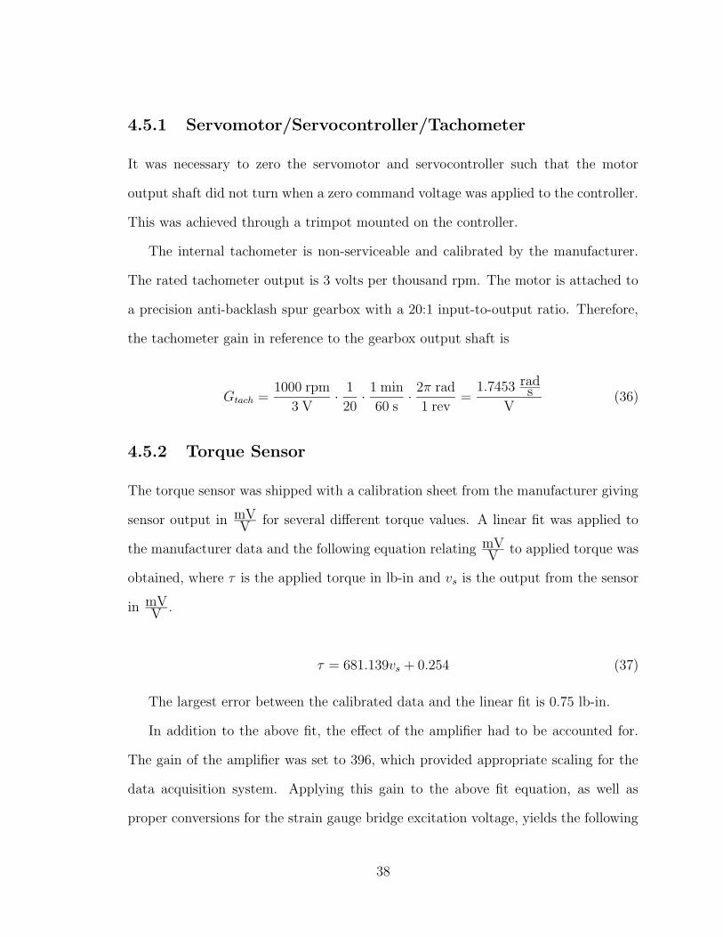
24 Typical Dynamic Clutch Torque Test . . . . . . . . . . . . . . . . . . 49

25 Measured Dynamic Clutch Torque . . . . . . . . . . . . . . . . . . . . 50

26 Measured Dynamic Clutch Torque with Individual Quadratic Fits . . 50

27 Measured Dynamic Clutch Torque with Single Scaled Quadratic Fit . 52

28 Final Dynamic Clutch Torque Model . . . . . . . . . . . . . . . . . . 53

29 Typical Breakaway Torque Test Data . . . . . . . . . . . . . . . . . . 54

30 Typical Breakaway Torque Test Data - Detail . . . . . . . . . . . . . 55

31 Breakaway Torques . . . . . . . . . . . . . . . . . . . . . . . . . . . . 56

32 Measured Breakaway Torques with Quadratic Fit . . . . . . . . . . . 58

33 Dynamic and Breakaway Torque Model Comparison . . . . . . . . . . 58

34 Model Comparison of the Two Clutch Tests . . . . . . . . . . . . . . 59

35 Tracking Error Definition . . . . . . . . . . . . . . . . . . . . . . . . . 62

36 Division of PTER’s Controller . . . . . . . . . . . . . . . . . . . . . . 64

37 SimPTER Output - Tip Position Plot - Baseline Test . . . . . . . . . 65

38 SimPTER Output - Clutch Velocities - Baseline Test . . . . . . . . . 65

39 SimPTER Output - Linear Tip Jerk and Clutch Velocities - Baseline

Test . . . . . . . . . . . . . . . . . . . . . . . . . . . . . . . . . . . . 67

40 SimPTER Output - Linear Tip Jerk and Acceleration - Baseline Test 67

41 Clutch Controller with Proportional Torque Feedback . . . . . . . . . 68

42 Clutch Controller with Proportional Torque Feedback - SimPTER Im-

plementation . . . . . . . . . . . . . . . . . . . . . . . . . . . . . . . 68

43 Proportional Torque Feedback Controller - Position Tracking Perfor-

mance . . . . . . . . . . . . . . . . . . . . . . . . . . . . . . . . . . . 70

x

44 Proportional Torque Feedback Controller - Smoothness Measure . . . 70

45 Endpoint Position - Baseline and Proportional Torque Feedback Con-

troller . . . . . . . . . . . . . . . . . . . . . . . . . . . . . . . . . . . 71

46 Clutch 2 Torque Following - Baseline Controller . . . . . . . . . . . . 72

47 Clutch 2 Torque Following - P Feedback Controller (Gain=0.16) . . . 72

48 Implemented Torque Controller - With and Without P Feedback . . . 74

49 Implemented Proportional Feedback Controller (gain=0.20) - Unstable

Behavior . . . . . . . . . . . . . . . . . . . . . . . . . . . . . . . . . . 75

50 Simulation of Testbed Torque Feedback Controller . . . . . . . . . . . 76

51 Desired Velocity Determination - Implemented Gomes Velocity Con-

troller . . . . . . . . . . . . . . . . . . . . . . . . . . . . . . . . . . . 77

52 Desired Velocity Determination - Proposed Velocity Controller . . . . 77

53 Instantaneous Generated Clutch Force Vectors . . . . . . . . . . . . . 79

54 Impedance and Velocity Controller Comparison - Endpoint Position . 81

55 Impedance and Velocity Controllers - Linear Tip Acceleration Magnitude 82









xi

Summary

This work studies the performance and control of a passive haptic display. The device

is passive in the sense that all its actuators are dissipative— they may only remove

energy from the system. All energy entering the system must be supplied by a human

operator. The purpose of the device is to exert forces on this operator. A dynamic

simulation of the device is enhanced through the addition of an actuator model in-

corporating dynamic response and friction behavior. Experimental data on actuator

performance is gathered and used to improve the accuracy of the new actuator model.

The simulation is then used to evaluate the performance of two new control concept-

s. One of these concepts is implemented on a testbed, and experimental results are

presented.

xii

Chapter 1

Introduction

1.1 The Haptic Display

The word haptic is one unfamiliar to most. It comes from the Greek haptesthai,

meaning “to touch,” defined as relating to or based on the sense of touch. A haptic

display is a device that interacts with a user through his or her sense of touch. Just

as a computer monitor is a visual display and a set of headphones is an aural display,

a haptic device is a touch display. There are many uses for such displays in the fields

of teleoperation, artificial environments (virtual reality), and ergonomics.

One of the first applications of haptic displays was in teleoperation. Tactile feed-

back can improve the performance of a local operator manipulating a remote system.

Such a system relies on the user projecting his dexterity into the remote environ-

ment. Although humans rely highly on visual cues to perform tasks, we also depend

on tactile cues for object identification and manipulation. [10] In situations where

visual sensing is impaired it can actually be replaced by tactile sensation. [8] Also, a

more accurate representation of the remote environment will instill a greater sense of

presence in the user, which may improve his or her performance. [20]

Virtual reality is another application of haptic displays. Force feedback can deliver

a third sense along with sight and sound to the virtual experience. There are a

wealth of applications in this field, including prototype visualization for CAD, virtual

1

evaluation and testing of factory layout and process flow, haptic input devices, and

of course entertainment. In fact it is entertainment that has started to deliver the

haptic display into the mainstream, evidenced by the latest force-feedback joysticks

now available for home computers.

In addition to their force reflection capabilities, haptic displays can also be used for

path guidance. In this application, the device tries to guide the user along a specific

path and/or constrain movement within a certain region. One such application would

be to aid the physically disabled, for example to facilitate walking in a paraplegic by

controlling limb movement. [9]

1.2 Passive Haptic Displays

Most existing haptic displays are active, comprised of actuators that can do positive

or negative work on the interfaced system. However, some current research involves

the study of passive haptics. [7] [14] [15] [18] A passive haptic display has no actuators

that can add energy to the system. That is, all energy added to such a device must

come from the user. Such a device has a primary advantage of safety over a similar

active device. Uncommanded movement is less probable in passive devices and is in

general easier to prevent. This makes passive haptics ideal for applications where

safety has high priority, such as assisted surgery and situations where high contact

forces are possible.

Passive haptic displays are a challenge to control, since arbitrary control actions

are not possible. A control action which adds energy to the system is not achievable.

An effective controller must determine whether or not desired control actions are

unachievable, and if so, define an achievable set of command inputs which act as a

2

compromise between system performance and realizability.

1.3 Organization of This Work

This work explores the enhancement of a simulation of a passive haptic display and its

subsequent use in the evaluation of control concepts that may increase system perfor-

mance. This chapter has provided some introductory information on haptic displays.

Chapter 2 reviews previous work done in the design and manufacture of a two degree-

of-freedom passive haptic testbed, the Passive Trajectory Enhancing Robot (PTER).

Chapter 3 explains the enhancement of a dynamic simulation of PTER through mod-

eling of stick-slip friction and actuator dynamics. Chapter 4 deals with the design

and manufacture of an actuator testbed used to perform system identification tests

on one of PTER’s four actuators, with the intent of building an actuator model for

use in the dynamic simulation. Chapter 5 addresses the implementation and simu-

lated performance of two new control concepts. Experimental results for one of these

control concepts are also presented. Finally, Chapter 6 contains closing comments

about the contribution of this work and some ideas for further research.

3

Chapter 2

Background

2.1 Development of PTER

2.1.1 PTER - Physical Description

An experimental passive haptic testbed has been built and used by previous students

for the purpose of studying the behavior of such a device and to evaluate control

techniques. [6] [11] This device has been named PTER— the Passive Trajectory

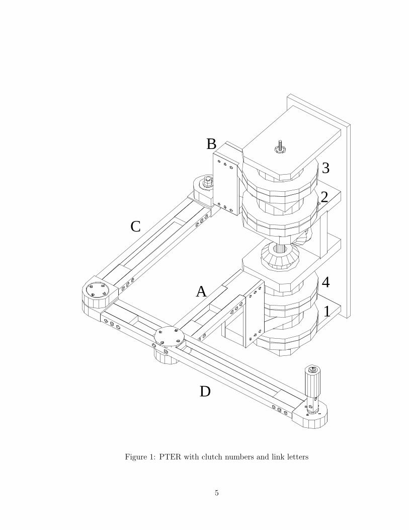
Enhancing Robot. Figure 1 is a diagram of PTER. It is a planar robotic arm in a

five-bar parallel linkage arrangement.

PTER’s purpose is to exert forces on the hand of a user, who grips the handle at

the endpoint of link D. It does this by providing torques to links A and B through

its network of four actuators. The actuators are controllable friction clutches. The

clutches are passive devices, only serving to remove energy from the system, hence

the passivity of the entire device. Clutch 1 and clutch 2 connect links A and B,

respectively, to ground. Clutch 3 couples the velocities of links A and B together.

Clutch 4 inversely couples links A and B together through the gears located in the

middle of the device. Since PTER has more clutches than degrees of freedom, the

robot is overactuated. This configuration was selected in order to provide greater

freedom in providing arbitrary torques to each of the main links A and B.

4

A

B

C

D

1

2

3

4

Figure 1: PTER with clutch numbers and link letters

5

In addition to its actuators, PTER contains several sensors. The handle mount

holds two strain gauges, used to measure the magnitude and direction of the user

applied force. Links A and B are each connected to potentiometers, which are used

to determine their positions. Since PTER has two degrees of freedom, the angles of

links A and B are sufficient to fully describe the state of the system.

2.1.2 PTER - Kinematic and Dynamic Equations

Kinematic and dynamic analysis of PTER have been sufficiently addressed by Charles

[4], Davis [6], and Gomes [11]. The pertinent equations will be summarized here and

the reader is referred to their work for the full derivations. These equations were used

in the development of the dynamic simulation of PTER later in this work. Figure

2 is a schematic diagram of PTER, showing the applicable coordinate systems and

parameter terminology.

Forward kinematics, transforming angular link position to global cartesian tip

position:

xtip = lA cos(θ1) − lD sin(θ2) (1)

ytip = lA sin(θ1) + lD cos(θ2) (2)

Inverse kinematics, transforming global cartesian tip position to angular link po-

sition:

q1 = arccos

(

x2 + y2 − l2A − l2D2lAlD

)

(3)

q2 = arcsin

(

[lA + lD cos(q1)]y − [lD sin(q1)]x

x2 + y2

)

(4)

θ1 = q2 (5)

θ2 = q1 + q2 +π

2(6)

6

θ1

θ2

lb

ld

rd

ar

rb

rc

x

y

D

Endpoint

t t(x , y )

l =lc a

A

B

C

Figure 2: PTER - dimensions and coordinate systems

7

Positions of coupling clutches 3 and 4:

θ3 = θ1 − θ2 (7)

θ4 = θ1 + θ2 (8)

It is a straightforward task to differentiate equations 8 with respect to time in order

to calculate the angular velocities and accelerations of the coupling clutches.

Velocity Jacobians relating link angular velocity and endpoint linear velocity:

x

y

=

−lA sin(θ1) −lD cos(θ2)

lA cos(θ1) −lD sin(θ2)

θ1

θ2

(9)

x

y

=1

2

−lA sin(θ1) + lD cos(θ2) −lA sin(θ1) − lD cos(θ2)

lA cos(θ1) + lD sin(θ2) lA cos(θ1) − lD sin(θ2)

θ3

θ4

(10)

Force Jacobian relating endpoint forces to clutch torques:

τ1

τ2

τ3

τ4

=1

2

−2lA sin(θ1) 2lA cos(θ1)

−2lD cos(θ2) −2lD sin(θ2)

−lA sin(θ1) + lD cos(θ2) lA cos(θ1) + lD sin(θ2)

−lA sin(θ1) − lD cos(θ2) lA cos(θ1) − lD sin(θ2)

fx

fy

(11)

The Jacobian matrices in Equations 10 may be inverted to obtain link velocities

from endpoint velocities. Since the Jacobian in Equation 11 is non-invertible, clutch

torques cannot be computed uniquely from a given endpoint force. This is due directly

to the fact that the system is overactuated.

The rigid-body equations of motion for the system, where rw is the distance from

the end of link w to its center of mass, mx is the mass of link x, Iy is the mass moment

of inertia of link y, and τz is the net torque on link z, are:

α =1

2

(

mArA2 + IA + IC + mCrC

2 + mDlA2)

(12)

8

β =1

2

(

mBrB2 + IB + ID + mC lB

2 + mD(rD − lB)2)

(13)

γ = mCrC lB − mDlA (rD − lB) (14)

2α γ sin(θ2 − θ1)

γ sin(θ2 − θ1) 2β

θ1

θ2

+

γθ22 cos(θ2 − θ1)

−γθ21 cos(θ2 − θ1)

=

τa

τb

(15)

2.1.3 Clutch Dynamics

The dynamics of PTER’s clutches have been briefly examined by Gomes [11]. His

experimental setup was less than ideal, and a satisfactory model was not obtained.

It was made clear, however, that the clutches act similar to a first-order system with

time delay, and that the lag and time constant of the system, though uncertain, are

sufficiently large to affect the control of the robot.

2.2 Control Methods

Since its inception, several controllers have been implemented on PTER. PTER’s

control needs can be separated into three parts. One controller must identify a set

of desired link torques given the instantaneous state of the system and its desired

behavior. The second controller must transform the desired link torques into a set

of achievable clutch torques, taking into account the system state and the clutches’

passivity constraint. Finally, the third controller must provide command signals to the

physical hardware in order to produce the torques desired by the second controller.

Most of the previous work in controlling PTER has concentrated on the first two

concepts. The latter task of generating control signals has been solved open-loop

through the use of a lookup table.

The initial controller as suggested by Charles [4] and implemented by Davis [6] is

9

an impedance controller, which computes desired tip forces through the simulation

of spring and damper elements between the endpoint of the robot and the desired

path. An algorithm named the “torque translator” was developed by Davis in order

to select a set of achievable clutch torques which match the desired link torques as

closely as possible. The signs of the clutch velocities are used to determine whether

or not a desired output torque is achievable.

Gomes looked into several different controllers with the aim of both improving

path following performance and minimizing tip acceleration [11]. He implemented a

simplified version of the torque translator, which considered desired tip forces rather

than desired clutch torques. High levels of tip acceleration due to rapid application

and release of clutches was evident. In light of this, Gomes implemented a blending

algorithm, which gradually applied and released clutches. This algorithm did not

significantly improve the tip acceleration profile. A controller using the tip velocity

rather than the position error was also investigated with promising results, though

the implementation was very basic.

2.3 Dynamic Simulation

A dynamic simulation of PTER was written in MATLAB by Charles [4]. In the

simulation the controller attempts to constrain the endpoint of the device to a circular

path. A force along the circle and a periodic normal disturbance force are applied to

the endpoint. The simulation computes net torque on links A and B by combining

required clutch torques with the user input force translated into link torques through

the Jacobian. The equations of motion are inverted and used to compute the link

accelerations from the net torques. Once the link accelerations are calculated, they

10

are integrated to obtain link velocity and position.

The Davis simulation was very rudimentary, having virtually no clutch modeling.

When the controller requested an arbitrary torque from a clutch, the simulation

assumed that the clutch immediately delivered exactly that torque. The only clutch

modeling lied in two checks:

• The requested torque must not exceed the maximum capacity of the clutch.

• The direction of the requested torque must not violate the passivity constraint

(i.e., must not add energy to the system.)

This simulation did a good job at basic validation of controller concepts, but

performed poorly at predicting the true behavior of the device, which is influenced

by factors not modeled in the equations of motion, such as friction effects and clutch

dynamics.

11

Chapter 3

SimPTER - Design and Development

3.1 Motivation for an Enhanced Simulation

Numerical simulation is a powerful tool for enhancing the design process of a multitude

of engineering systems. It allows one to evaluate different system configurations and

control concepts without having to physically construct the system. Often this yields

a cheaper, quicker, more straightforward, and safer development process.

It appears that PTER’s performance is limited by inherent nonlinearities in its

hardware— specifically stiction and stick-slip effects at the clutches’ friction interfaces

and in the finite gap between the clutch plates when the clutch is not applied. The

latter results in time lag and high initial-contact forces. Both of these nonlinearities

create a “jerky” feel to the user. In order to facilitate the study of control systems

and possible alternative actuators, it was decided to enhance the dynamic simulation

by implementing a more accurate model of PTER.

This chapter provides an overview of the extensive changes made to the original

simulation, called SimPTER. The bulk of this work was done at ENSAM Paris,

France, with the help of Eric Romagna under the tutelage of Professor Andre Barraco.

[17]

12

3.2 SIMULINK Implementation

In the end, the new SimPTER was an almost complete rewrite of the original. There is

very little in common between the two simulations. The only parts that carried over to

the new simulation were the control code and several functions describing the dynamic

properties of PTER. These functions do things such as Jacobian transformations and

inverse dynamics computation. From this point on, the name SimPTER will apply

to the new simulation.

The previous simulation was essentially a group of MATLAB M-files which were

run from the command line. Since the simulation would eventually be used to evaluate

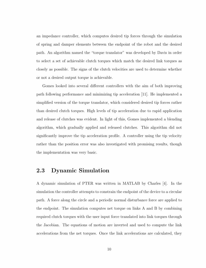
different system configurations, it was decided to implement SimPTER in SIMULINK

in order to take advantage of its GUI and improved usability. Figure 3 is a diagram

of the SimPTER SIMULINK model. The model is composed of four main blocks:

• Input Tip Force — This block models the input force.

• Controller — This block contains the controller.

• Clutch Model — This block comprises the entire clutch model, including both

dynamic response and nonlinear friction properties.

• Dynamic Simulation — This block contains all dynamic information about

PTER and computes its full state based on the net torque applied to each

link.

The remainder of this section more thoroughly explains the purpose and function

of these blocks.

13

taue

TorqueVector

Current Tau 4Current Tau 3Current Tau 2Current Tau 1

Last Tau 4Last Tau 3Last Tau 2Last Tau 1

TorqueMemory

0

TimeDisplay

STOP

Stop Simulation

timeSimulation

Time

PulseGenerator

Net Torqueon Arm 2

Net Torqueon Arm 1

model_caseModel Cases

theta1

theta2

time

Applied Torques

x force

y force

Input Tip Force

Mux

Input Force(2)/Position(2)/Velocity(2)/

Time

Mux

GeneratedBrake Torques

model_errorError in Brake Model

Net Torque 1

Net Torque 2

Position 1

Position 2

Vel 1

Vel 2

Pre Vel 1

Pre Vel 2

Dynamic Simulation

tau_d

DesiredTorques

Input VectorClutch 1 Actual TorqueClutch 2 Actual TorqueClutch 3 Actual TorqueClutch 4 Actual Torque

Voltages (4)

Desired Torques

Controller

command_voltagesCommanded

Voltages

tau_in1tau_in2Control Voltagestheta1theta2Pre Vel 1Pre Vel 2tau4_prevtau3_prevtau2_prevtau1_prev

Generated Torques/ status

Clutch Model

Clock

Demux

BrakeTorques(4)/

Model Errors

app_torqueApplied Torques

Demux

AppliedTorques

Fig

ure

3:Sim

PT

ER

2-SIM

ULIN

KM

odel

14

3.2.1 Input Tip Force

This block provides the simulation with the tip forces and resultant link torques gen-

erated by the virtual user on PTER’s handgrip. Currently, the force is modeled as

having a constant component parallel to the desired path and a tangent component

comprised of a summation of sinewaves. This input was chosen to provide a distur-

bance force to the tip of the robot, without singling out a single frequency which

could lead to instabilities or lockup conditions within the controller.

3.2.2 Controller

This block is comprised of all three components mentioned in the previous chapter.

That is, one component computes desired link torques, the second transforms the

desired link torques into achievable clutch torques, and the third provides command

signals to the physical hardware (which is, in this case, the clutch model.) The

controller initially implemented in the simulation is the impedance controller and

torque translator mentioned in the previous chapter, combined with a simple piecewise

linear torque-voltage model to provide open-loop torque control. This look-up table

method to compute command voltages was used because it is the same method used

in the physical setup.

3.2.3 Clutch Model

This block contains the model of PTER’s clutches. The two parameters of the clutches

that were to be modeled were the dynamics and the friction behavior.

15

3.2.3.1 Clutch Dynamics

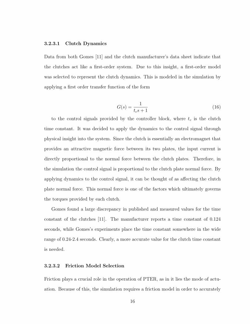
Data from both Gomes [11] and the clutch manufacturer’s data sheet indicate that

the clutches act like a first-order system. Due to this insight, a first-order model

was selected to represent the clutch dynamics. This is modeled in the simulation by

applying a first order transfer function of the form

G(s) =1

tcs + 1(16)

to the control signals provided by the controller block, where tc is the clutch

time constant. It was decided to apply the dynamics to the control signal through

physical insight into the system. Since the clutch is essentially an electromagnet that

provides an attractive magnetic force between its two plates, the input current is

directly proportional to the normal force between the clutch plates. Therefore, in

the simulation the control signal is proportional to the clutch plate normal force. By

applying dynamics to the control signal, it can be thought of as affecting the clutch

plate normal force. This normal force is one of the factors which ultimately governs

the torques provided by each clutch.

Gomes found a large discrepancy in published and measured values for the time

constant of the clutches [11]. The manufacturer reports a time constant of 0.124

seconds, while Gomes’s experiments place the time constant somewhere in the wide

range of 0.24-2.4 seconds. Clearly, a more accurate value for the clutch time constant

is needed.

3.2.3.2 Friction Model Selection

Friction plays a crucial role in the operation of PTER, as in it lies the mode of actu-

ation. Because of this, the simulation requires a friction model in order to accurately

16

−FB

FB

V

Ff

Figure 4: Stick-Slip Friction Model

M

-

-

�

/////////////////

V

Fin

Ff

Figure 5: Simple One-Mass Friction System

represent the behavior of the system. A literature search was performed to identify

possible candidate numerical friction models. Several models were evaluated, includ-

ing the Dahl [5], reset-integrator, and bristle models [12]. In the end, the Karnopp

friction model [13] was selected due to its clean separation of static and dynamic be-

havior, ability to model important nonlinearities such as high breakaway forces, and

acceptable computation requirements. The reset-integrator model was also seriously

considered, but was found more difficult to implement within the existing simulation

framework than the Karnopp model.

Stick-slip friction is a discontinuous phenomenon (see Figure 4.) It consists, how-

ever, of two separate modes, each of which is piecewise continuous for a specific system

17

∫∫

vDvD−

vD−

vD

hF−

hF

m

1 ∫

stickF

slipF

F

fF

rV x

vD−

vD

-

+

+

+

Figure 6: Karnopp Friction Model - Block Diagram

variable. The applicable mode at any point in time depends on whether or not there

is relative velocity between the two friction surfaces. The Karnopp model utilizes

different sets of governing equations for each of these modes. In effect, the order of

the dynamic system is reduced when the relative velocity is equal to zero. Within

this reduced-order framework, the position constraint of zero relative velocity is in-

corporated into the system of differential equations. This provides a practical means

of dealing with the friction force discontinuity at zero relative velocity. For a simple

single-mass system such as that in Figure 5, the Karnopp model yields the system

shown in Figure 6 and the following equations for frictional force Ff :

Ff =

g(V ) : |V | ≥ δV

Fin : |V | < δV, Fin ≤ FB

FB : |V | < δV, Fin > FB

(17)

18

When the magnitude of the relative velocity V between the two surfaces is greater

than or equal to a very small value δV , the system is said to be in the slip mode.

Even though the system is physically slipping when V is not equal to zero, the nonzero

region around V = 0 is defined in order to account for close-to-zero errors. In the slip

mode the friction force is dependent only on the relative velocity, and is determined

by an arbitrary function g(V ).

When the magnitude of the relative velocity V between the two surfaces is less

than δV , the system is said to be in the stick mode. In the stick mode the system

is static, and the friction force Ff exactly cancels the driving force Fin, unless Fin

exceeds the breakaway force FB. In the latter case the Ff is equal to FB and the

body will experience nonzero acceleration. After a short interval the magnitude of V

will exceed δV and the model will transition from the stick mode to the slip mode.

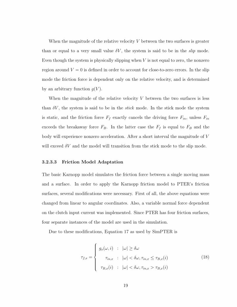
3.2.3.3 Friction Model Adaptation

The basic Karnopp model simulates the friction force between a single moving mass

and a surface. In order to apply the Karnopp friction model to PTER’s friction

surfaces, several modifications were necessary. First of all, the above equations were

changed from linear to angular coordinates. Also, a variable normal force dependent

on the clutch input current was implemented. Since PTER has four friction surfaces,

four separate instances of the model are used in the simulation.

Due to these modifications, Equation 17 as used by SimPTER is

τf,x =

gx(ω, i) : |ω| ≥ δω

τin,x : |ω| < δω, τin,x ≤ τB,x(i)

τB,x(i) : |ω| < δω, τin,x > τB,x(i)

(18)

19

where x = 1 . . . 4 represent the four clutches, and i is the input current to each

clutch. Notice that all forces from the initial model are replaced with torques, and

linear velocity has been replaced with angular velocity.

3.2.3.4 Clutch Model Implementation

After a numerical friction model was selected and tailored to the specific case of

simulating PTER, it was necessary to implement it. The goal of the clutch model is

to calculate generated clutch torques given input signals and the state of the system.

The Karnopp model will yield this information, as the frictional force represented in

the model is actually the generated clutch torque. Since the Karnopp model contains

two distinct modes (stick and slip), there will be two different methods for calculating

an arbitrary generated clutch torque, dependent on the clutch’s dynamic mode. The

code determines the dynamic mode of each clutch based on its relative plate velocity

ω. If ω is within the range [−δω, δω] then it is considered to be in the stick mode,

otherwise it is in the slip mode. If a clutch has zero input current, its reaction torque is

assumed to be zero, regardless of its dynamic mode. This was done to greatly simplify

the model code, and is a valid assumption since the zero-current torque generated by

PTER’s clutches is very nearly zero.

In the slip mode, torque calculation is straightforward. According to the modified

Karnopp model equation 18, the reaction torque is dependent only on the input

current furnished to the clutch and the relative clutch plate velocity. A dynamic

friction model for the clutches is used to compute the reaction torque. For solely

friction model validation purposes, a linear model from zero to maximum rated clutch

torque was used.

Torque calculation for the stick mode is more involved. In this case, the modified

20

Case # Clutch 1 Mode Clutch 2 Mode Clutch 3 Mode Clutch 4 Mode1 slip/NA slip/NA slip/NA slip/NA2.1 stick slip/NA slip/NA slip/NA2.2 slip/NA stick slip/NA slip/NA3.1 slip/NA slip/NA stick slip/NA3.2 slip/NA slip/NA slip/NA stick4.1 stick NA stick NA4.2 stick NA NA stick4.3 NA stick stick NA4.4 NA stick NA stick5 stick stick NA NA6 NA NA stick stick7 stick stick stick stick

Table 1: The 12 Possible Modes of PTER (N/A = not applied)

Karnopp model equation 18, shows that the reaction torque is dependent on the input

current furnished to the clutch and the net external torque applied to the clutch. It is

therefore clear that the net external torque applied to the clutch must be computed.

In order to do this, the equations of motion of the system are solved under special

circumstances depending on the specific system state. It is assumed that if a clutch

is in the stick mode, it will remain immobile until the net external torque applied to

it exceeds its static breakaway level. Given this assumption, the equations of motion

can be simplified and solved for the clutch torques required to keep the static clutches

in the stick mode. This concept is made more clear by example below.

The net torque on each link is the summation of clutch reaction torques and input

forces transformed into torques:

τA = τ1 + τ3 + τ4 + τA,ext (19)

τB = τ2 − τ3 + τ4 + τB,ext (20)

Therefore, the equations of motion of the system (Equation 15) can be written as

21

follows:

M11 M12

M21 M22

θA

θB

+

V1

V2

=

τ1 + τ3 + τ4 + τA,ext

τ2 − τ3 + τ4 + τB,ext

(21)

where the Mxy values represent PTER’s inertial matrix, θx is the angular accel-

eration for link x, and the Vx values account for velocity-dependent coupling effects.

There are twelve possible dynamic modes that PTER can be in (24 possible from the

Karnopp model with four surfaces, minus four unachievable states due to the fact

that the system is overactuated, such as clutch 1 slipping and clutches 2, 3, and 4

sticking.) These possible modes are listed in Table 1. We will consider Case 2.1 to

furnish an example.

In Case 2.1, clutch 1 is in the stick mode and all others are in the slip mode. The

calculation of the generated clutch torques for clutches 2, 3, and 4 is straightforward

as discussed above. The torque required of clutch 1 to keep itself static is solved by

setting its relative angular acceleration to zero and solving the equations of motion

for torque. Otherwise, if

θA = 0 (22)

then the equations of motion yield

τ1 =(

M12

M22

)

τ2 −(

M12

M22

+ 1)

τ3 +(

M12

M22

− 1)

τ4

+(

M12

M22

)

τinB − τinA + V1

(23)

If the computed τ1 is below the breakaway torque for clutch 1, then the code

returns τ1 for the generated torque and the clutch remains stuck. However, if it

is above the breakaway torque, then the code returns the breakaway torque as the

22

generated torque and the clutch will eventually start to slip. See Appendix A for the

full set of calculations required for each of the modes listed in Table 1.

The primary limitation of this method is that it cannot be used for Case 7. Case

7 represents all situations where all velocities are zero and three or four clutches are

applied. In these cases there are three or four unknown static torques to be found,

but only two equations of motion. This yields a statically indeterminate system. In

order to deal with Case 7, an alternate method of computing clutch torques had to

be found.

The method devised to deal with Case 7 was named the lumped actuator approach.

In effect, the order of the system is reduced by considering not the four clutches

independently, but as a lumped set acting on the two main links A and B. At the lowest

level, all that the simulation requires from the clutch model is the net torque acting

on each of the two links A and B due to the system of clutches. It is advantageous to

compute the contribution of each clutch for informational and analysis purposes, and

even necessary when clutches are slipping. However, in Case 7 the entire system is

static, since more than one clutch is stuck, thus reducing PTER to a zero degree-of-

freedom device. The goal of the simulation at this point is to determine whether or

not the system will remain at zero degrees-of-freedom and if not, what part(s) of the

robot will start moving. To this end, the lumped actuator approach considers all the

applied clutches as a single actuator which will supply appropriate torques to links A

and B, up to a certain breakaway level, in order to keep the system fully static. At

this point the question remains: how to determine whether or not the lumped set of

clutches is capable of keeping the system static, and if not, in what fashion will the

robot start to move?

Case 7 is divided into five subcases, as shown in Table 2. The implementation of

23

Case # Clutch 1 State Clutch 2 State Clutch 3 State Clutch 4 State7.1 applied applied applied free7.2 applied applied free applied7.3 applied free applied applied7.4 free applied applied applied7.5 applied applied applied applied

Table 2: Case 7 Subcases

the lumped actuator approach for subcase 7.1 will be explained, with understanding

that the other cases are treated in a similar fashion.

For Case 7.1, clutch 4 is free and need not be considered. Several special cases

of the equations of motion are defined with the intent of putting the equations of

motion into a solvable form. Three cases are defined, each with one of the applied

clutch torques set to its breakaway level. The torques required of the remaining

two clutches to keep the system fully static can then be computed. The following

equations are the results of the solved equations of motion for each of these special

cases for Case 7.1.

τ13 = −τinA − τ1,breakaway (24)

τ12 = −τinB + τ13 (25)

τ23 = τ2,breakaway + τinB (26)

τ21 = −τ23 − τinA (27)

τ31 = −τinA − τ3,breakaway (28)

τ32 = −τinB + τ3,breakaway (29)

where τxy is defined as the torque required of clutch y to keep the system static if

clutch x is at its breakaway level.

It is assumed that if the system of actuators is able to keep the system fully static,

24

that is, there exists any feasible combination of clutch torques to this end, then the

system will remain fully static. Therefore if any of the three cases listed above yields

both resultant torques below their breakaway levels, then the system will remain

completely static. It is important to realize that when this approach is used, the

clutch torques returned by the model have no physical meaning whatsoever. They do

not represent the actual torques produced by the clutches. What they do represent

is a means by which the two correct net link torques can be computed. With the

lumped actuator approach, the net link torques will be correct, while the component

clutch torques which comprise the net torques will not.

In the event that one of the above special cases is not valid, it is assumed that the

system will transition to a dynamic state. Now the question is how many clutches

will slip, and which ones? If none of the six torques computed above are below their

respective breakaway torques, it is assumed that every clutch will start to slip. In

this case, the model outputs the breakaway torque of each clutch as their generated

torques. If at least one of the six computed torques is below its breakaway level,

then the previous timestep’s torques for each clutch are used to determine which two

clutches will slip. The two clutches with previous torque values closest to breakaway

are the ones that will slip. When the two clutches to slip have been identified, the

breakaway torques for those clutches are output by the model, and the torque for the

third clutch will be computed through the now-solvable equations of motion, similar

to the solutions of Cases 2 and 3.

Of course, it is obvious to ask whether or not using the previous timestep’s clutch

values is a valid method, since it has been established that these values have no

physical significance in and of themselves. However, if the system is fully static

and external forces are rising to the point of dynamic transition, it is apparent that

25

eventually only one of the special cases will produce a satisfactory condition, i.e. both

computed torques are below breakaway levels. In this case, even though the values of

the computed clutch torques are not valid, the general magnitudes are; one clutch will

be at or near breakaway and the system will slip when a second reaches breakaway. It

can be assumed that the two clutches closest to their breakaway values will ultimately

slip. In the case that the timesteps are very large, and there are two or more valid

cases carried over from the previous timestep, it is impossible to guess which clutches

will slip, and one guess is as good as any.

As stated above, the implementation of the lumped actuator approach for the

other subcases of Case 7 are similar. The exception is subcase 7.5, in which six

special cases are needed instead of three, since two clutch torques must be defined

in order to render the equations of motion solvable. After the definition of these six

special cases, the logic of the solution is the same.

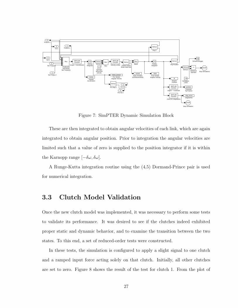
3.2.4 Dynamic Simulation

Figure 7 is a diagram of the dynamic simulation portion of SimPTER. This block

computes PTER’s full dynamic state— the angular position, velocity, and acceleration

of links A and B. The inputs to the block are the net torques on each link, calculated

from the input forces and the generated clutch torques, the latter being supplied by

the clutch model.

The block first uses the equations of motion (see Equation 15) to compute the

angular accelerations of each link as follows:

θA

θB

=

M11 M12

M21 M22

−1

τA

τB

−

V1

V2

(30)

26

6

Pre Vel 2

5

Pre Vel 1

4

Vel 2

3

Vel 1

2

Position 2

1

Position 1

MATLABFunction

torque−−>acceleration

sing_errors

singularities

MATLABFunction

check for singularities

MATLABFunction

angles−−>cartesian

MATLABFunction

Velocity Limiter

1/s

VelocityIntegrator

STOP

Stop Simulation1

STOP

Stop Simulation

locked

State of brakes(locked/unlocked)

−26

Simulationx limit

Schwarzenegger

<=

RelationalOperator

thdot_unmod

Pre−limitedAngular Velocity

Demux

Pre Ang V

thdot

Post−limitedAngular Velocity

Mux

Position(2)/Velocity(2)/

Net Torque(2)

1/s

PositionIntegrator

Mux

Mux6Mux

Mux

Demux

Limited Vel(2)/Brake state bytedv

Karnoppdifferential

velocity

Demux

Demux1

Demux

Demux

position

CartesianTip Position

th

AngularPosition

th2dot

AngularAcceleration

Demux

Ang V

Demux

Ang Position

2

Net Torque 2

1

Net Torque 1

Figure 7: SimPTER Dynamic Simulation Block

These are then integrated to obtain angular velocities of each link, which are again

integrated to obtain angular position. Prior to integration the angular velocities are

limited such that a value of zero is supplied to the position integrator if it is within

the Karnopp range [−δω, δω].

A Runge-Kutta integration routine using the (4,5) Dormand-Prince pair is used

for numerical integration.

3.3 Clutch Model Validation

Once the new clutch model was implemented, it was necessary to perform some tests

to validate its performance. It was desired to see if the clutches indeed exhibited

proper static and dynamic behavior, and to examine the transition between the two

states. To this end, a set of reduced-order tests were constructed.

In these tests, the simulation is configured to apply a slight signal to one clutch

and a ramped input force acting solely on that clutch. Initially, all other clutches

are set to zero. Figure 8 shows the result of the test for clutch 1. From the plot of

27

Constant DOFActual Path

-40 -30 -20 -10 0

0

5

10

15

20

25

30

X (in)

Y (in

)

SimPTER Endpoint Position

0 1 2 30

20

40

60

80Brake 1 Generated Torque (in-lbs)

Time (s)0 1 2 3

-1

-0.5

0

0.5


Time (s)

0 1 2 3-1

-0.5

0

0.5


Time (s)0 1 2 3

-1

-0.5

0

0.5


Time (s)

Figure 8: Reduced Order Test - Clutch 1

-40 -30 -20 -10 0

0

5

10

15

20

25

30

X (in)

Y (in

)


0 1 2 30

20

40

60


Time (s)0 1 2 3

0

5

10


Time (s)

0 1 2 3-1

-0.5

0

0.5


Time (s)0 1 2 3

-1

-0.5

0

0.5


Time (s)

Figure 9: Reduced Order Test - Clutch 1 with Clutch 2 Locked

generated torque for clutch 1, it can be seen that the generated torque is ramping

up to compensate for the ramped input force, and clutch 1 remains stuck. When the

input torque to clutch 1 exceeds its breakaway torque (65 in-lbs in this case), then the

clutch slips and transitions to the slip mode. Since the dynamic friction model used

for these tests is independent of clutch plate velocity, the model outputs a constant

generated torque while the clutch is slipping. In the endpoint plot, the dotted line

represents the path that PTER’s tip would take if only clutch 1 was moving. It does

not exactly follow the path in this case due to the velocity coupling terms Vx in the

equations of motion causing link B to move as well.

28

Another test was performed on clutch 1 with the same parameters, except now

clutch 2 is supplied with a maximum input signal. This should eliminate the move-

ment of link B after clutch 1 starts to slip as evidenced in the above test. The results

are in Figure 9, and it can be seen that the endpoint now follows exactly the sin-

gle degree-of-freedom line. In this case, clutch 2 generates torque to counteract the

influence of the Vx terms, and keeps link B static.

The same tests were performed on the other clutches, all with similar results. See

Appendix B for the results of these tests.

3.4 Required Changes to SimPTER

At this point, it has been shown that a dynamic simulation of PTER with a valid ac-

tuator model has been developed. In order to use SimPTER to make judgments about

proposed changes to the physical system, accurate models for the clutch dynamics

and static and dynamic friction forces must be added.

29

Chapter 4

PTER - Actuator Identification and

Modeling

4.1 Motivation for System Identification

After the framework dynamic clutch model had been fully implemented in the dy-

namic simulation of PTER, it was necessary to add models for relevant physical

phenomena in order to make the simulation as accurate as possible. Prior to this

point, very rudimentary models relating generated dynamic clutch torque and break-

away torque to input voltage were available. Data on the first order time constant of

the clutches was inconclusive. Due to these factors, it was decided that more accu-

rate information was required, and to perform system identification tests on PTER’s

clutches.

4.2 Previous Testing

Gomes performed several tests on the clutches in an attempt to characterize the

friction and dynamic properties. [11] These tests were performed with the clutches in-

place in order to avoid disassembly of PTER and the construction of testing hardware.

Two types of tests were performed by Gomes— a breakaway torque test for each

clutch and dynamic response tests of a single clutch. The breakaway torque tests

30

consisted of setting one of the clutches at a constant input voltage and applying force

to the tip of PTER until the locked clutch slipped. The input force at the onset of

slip was transformed into a set of link torques, and the breakaway torque for the given

clutch was computed.

The dynamic response tests consisted of a user moving the tip of PTER with no

clutches applied and applying a step input voltage to the clutch. The user attempted

to keep the applicable link moving at a constant velocity. Again, generated clutch

torque was computed by transforming applied tip force into applied link torques. The

time response of the clutch torque was then used to obtain a first-order time constant

for the system. A time delay was also noted in the clutch response. Frequency

response analysis was also performed by feeding a biased swept sinewave voltage to a

specific clutch and again attempting to move the particular link at a constant velocity.

Gomes obtained widely differing values for the time constant in the range of 0.25

to 2.5 seconds from the step response and frequency response tests. It is difficult to

determine a valid time constant from this data for use in the simulation.

For the first implementation of SimPTER, the existing model for breakaway torque

was used. Several time constants were utilized within the range identified by Gomes.

Models for generated dynamic torque were created by extracting the torque-to-voltage

model from the PTER control code and inverting it to obtain a voltage-to-torque

model.

4.3 Initial In-Place Testing

At this point, better data was needed to characterize the behavior of the clutches.

It was decided to perform some additional in-place tests on a clutch for the primary

31

AmplifierStrain Gauge

LabVIEWComputer

Power Supply

PositionPotentiometer

F

ω

Clutch

Torque Bar

Strain Gauges

D/A

A/D

A/D

Figure 10: Torque Bar Test - Experimental Setup

purpose of characterizing its dynamic friction properties. When the tests were being

planned, PTER had been partially disassembled by another student for other pur-

poses. This partial state of disassembly allowed more flexibility in deciding how the

tests would be performed.

It was decided to utilize a long aluminum bar approximately 36” x 3” x 0.25” to

apply torque to a clutch. Three holes were drilled in the bar, and it was attached to

the clutch by bolting it to PTER’s preexisting hardware. Strain gauges were mounted

on the 3” face of the bar. By measuring the strain in the bar, the applied torque

was computed. This method has the advantage over Gomes’s in-place experiments

in that the generated clutch torque is directly measured rather than computed from

the tip input forces.

The tests consisted of applying a constant input voltage to the clutch and manually

applying force to the bar until the clutch started to slip. After slip occurred, the user

attempted to keep the clutch moving at a constant velocity through approximately

90 degrees of travel. In addition to measuring dynamic torque, this method had the

added benefit of measuring breakaway torque. See Figure 10 for a diagram of the

32

experimental setup used for these tests.

This test provided data showing that the relationship between clutch torque (both

dynamic and breakaway) and the clutch input voltage is a quadratic one (see Figures

11 and 12). The fit that was ultimately selected is in fact a modified quadratic. It

has a linear section that passes through the origin and the point of zero slope on the

fitted quadratic. This was done for two reasons. First of all, the quadratic function

decreases as voltage increases in the low voltage range, left of the point of zero slope,

which does not accurately match the model. Second of all, a zero value of torque

when zero input voltage is applied is desirable, both because it matches the actual

behavior of the system and it simplifies the numerical friction model.

Gomes assumed a linear piecewise fit for his data, even though it appears to

follow a more quadratic behavior. Some physical insight into the structure of the

clutches provides an explanation for the quadratic fit. Each clutch is in essence

an electromagnet, with friction material between a coil section and a ferric section.

Electrically, the system is an RL circuit. The energy consumed by the coil may be

written as the time integral of the power:

E =∫

P dt =∫

V i dt (31)

which can be further reduced to:

∫

Lidi

dtdt =

∫

Li di =1

2Li2 (32)

By using the concept of virtual work, the normal force N produced by the system

can be computed as follows:

33

0 5 10 15 200

50

100

150

200

250

300

350

400

450Clutch Dynamic Reaction Torque: Actual Values and Modified Quadratic Model

Clutch Input Voltage (volts)

Rea

ctio

n T

orqu

e (in

−lb

s)

Model Measured Values

Figure 11: Torque Bar Test - Dynamic Torque Data and Curve Fit

0 5 10 15 200

100

200

300

400

500

600

Clutch Input Voltage (volts)

Bre

akaw

ay T

orqu

e Le

vel (

in−

lbs)

Clutch Breakaway Transition Torque Level: Actual Values and Modified Quadratic Model

Model Measured Values

Figure 12: Torque Bar Test - Breakaway Torque Data and Curve Fit

34

δW = δE = Nδx (33)

N =δE

δx≈

dE

dx=

1

2

dL

dxi2 (34)

where x represents the air gap between the coil and ferric sections, and the assump-

tion is made that the current in the coil i is invariant with x. According to coulomb

friction theory, the frictional force generated by the clutch is directly proportional to

the normal force between the coil and ferric mass:

F = µN (35)

From the above equations, it is seen that the generated friction between the clutch

plates is directly proportional to the square of the input current. Such a relationship

with the input current will show a similar quadratic relationship with the input voltage

as long as the system is at steady state. During transient behavior, there are dynamic

factors based on the clutch’s electrical properties that affect the relationship between

clutch torque and input voltage.

4.4 Development of a Motorized Clutch Testbed

The in-place tests that were performed lent insight into the structure of the clutch

torque behavior, but the results were still not sufficient to build a reliable clutch

model. The input force was provided by a human, who cannot apply a constant

input torque. This seriously affects the validity of measured transient parameters of

the system. Inaccuracies in the model of the torque bar may influence the accuracy

of the collected torque data. Due to noise in the electrical system, torques at clutch

35

Clutch -Coil(Stationary)

Clutch - Ferric Portion(Rotating)

RotaryEncoder

ω

Torque Sensor

Driveshaft

Bearings

Motor

Supports

Base

Figure 13: Clutch System ID Testbed - Mechanical Layout

voltages below 12 volts, which is half-scale, could not be measured. Also, as seen in

the previous subsection, it would be better to build a model based on input current

rather than input voltage. Such a model would more accurately represent the system,

especially in the presence of transients. This is key in the current application, as

PTER’s clutches are rarely commanded a steady-state behavior.

It was decided that the simplicity of implementation of the in-place tests did not

outweigh the need for more accurate data, especially for the time constants and time

lags of the clutches. In this light, a separate testbed was developed in order to allow

36

more flexibility in applying torques to the clutches and more accuracy in measuring

clutch position and velocity as well as generated torques.

A servomotor, controllable in both velocity and torque, was selected to apply

torque to a clutch. The servomotor has an integrated analog tachometer used by

the servo controller which may also be interfaced to the data acquisition system. A

calibrated commercial reaction torque sensor was selected to measure the generated

clutch torque.

Figure 13 is a mechanical diagram of the testbed setup. The same computer and

data acquisition card that was utilized for the former test was used. LabVIEW was

again used to develop acquisition software. The torque sensor is an aluminum cylinder

with a full-bridge strain gauge circuit. When torque is applied, the cylinder is put

into torsion and the strain gauge bridge puts out a voltage directly proportional to the

applied torque. An Analog Devices strain gauge amplifier module was used to process

the signal, which was then fed to the acquisition computer. The output of the motor’s

tachometer was interfaced directly to an ADC channel of the acquisition board. For

control, two DAC channels were used to apply command voltages to the clutch power

supply and the servomotor controller. The servomotor controller is capable of both

torque and speed control. Both types of control were used for the tests in question.

4.5 Testbed Setup and Calibration

It was necessary to calibrate the electronics on the testbed before commencing tests.

This section describes the process followed for those components requiring calibration

as well as the equations used to convert signals into physical measurements.

37

4.5.1 Servomotor/Servocontroller/Tachometer

It was necessary to zero the servomotor and servocontroller such that the motor

output shaft did not turn when a zero command voltage was applied to the controller.

This was achieved through a trimpot mounted on the controller.

The internal tachometer is non-serviceable and calibrated by the manufacturer.

The rated tachometer output is 3 volts per thousand rpm. The motor is attached to

a precision anti-backlash spur gearbox with a 20:1 input-to-output ratio. Therefore,

the tachometer gain in reference to the gearbox output shaft is

Gtach =1000 rpm

3 V·

1

20·1 min

60 s·2π rad

1 rev=

1.7453 rads

V(36)

4.5.2 Torque Sensor

The torque sensor was shipped with a calibration sheet from the manufacturer giving

sensor output in mVV for several different torque values. A linear fit was applied to

the manufacturer data and the following equation relating mVV to applied torque was

obtained, where τ is the applied torque in lb-in and vs is the output from the sensor

in mVV .

τ = 681.139vs + 0.254 (37)

The largest error between the calibrated data and the linear fit is 0.75 lb-in.

In addition to the above fit, the effect of the amplifier had to be accounted for.

The gain of the amplifier was set to 396, which provided appropriate scaling for the

data acquisition system. Applying this gain to the above fit equation, as well as

proper conversions for the strain gauge bridge excitation voltage, yields the following

38

−8 −6 −4 −2 0 2 4 6 8−1500

−1000

−500

0

500

1000

1500Torque Sensor Calibration − Actual Data and Linear Fit

Amplifier Output Voltage (V)

Mea

sure

d T

orqu

e

Linear Fit Manufacturer’s Calibration Data

Figure 14: Torque Sensor Calibration - Calibration Data and Linear Fit

equation for measured torque versus voltage input to the data acquisition computer:

τ = 171.988v + 0.254 (38)

Figure 14 is a graph of both the linear fit and the actual factory calibration data.

Instead of building an external circuit to zero the torque sensor output, data was

taken with zero torque input and the value of the torque sensor output for zero input

was subtracted from all subsequent data.

4.6 Clutch Testbed Experiments

The purpose of the clutch tests was twofold. First of all, the dynamic response of

the clutches was to be investigated. Secondly, a model of the friction behavior of the

clutches in both static and dynamic modes was to be built. This section explains

these two groups of tests and presents their results.

39

In all tests, the mechanical parameters being measured by analog transducers

have been filtered to eliminate excess electrical noise in the signal. It was determined

that the vast majority of electrical noise was caused by the servomotor controller. A

4th order digital Butterworth filter with a cutoff frequency of 150 Hz was used to

postprocess the sampled data from the torque sensor and the tachometer.

4.6.1 Clutch Dynamics

Several datasets were taken with a constant commanded motor speed and a step

input current commanded to the clutch. An important factor that directly affects

the results is that the power supply which drives the clutch cannot in fact provide a

sharp step input. This is due to the time it takes to build up current in the clutch

coil. Figure 15 shows the current commanded and actual current and voltage applied

to the clutch for a step input of 3 volts to the clutch (which has an input command

range of 0-10 volts). Figure 16 shows a similar plot for a step input of 8 volts. It is

clear from these figures that the actual current supplied by the power supply exhibits

a significant transient response. Also notice that the rise time of the current in the 8

V case is more than twice that of the 3 volt case. This is due to voltage saturation

of the power supply, which can also be observed by the flattened voltage response in

Figure 16. In fact, step inputs of higher than 8 volts could not be applied, as the

voltage would peak too high and set off the safety crowbar in the power supply.

With this insight into the power supply dynamics in mind, it is understood that

any transient response measured for the clutches will in fact be a combined response

of the clutch and power supply as a single system. This is not a severe limitation,

however. The clutch requires a power supply to operate, so they will always be used

together as a unit. Due to this fact, applying a combined dynamic model of both

40

1.95 2 2.05 2.1 2.15 2.2 2.25 2.3

0

0.5

1

1.5

2

2.5

3

3.5

Time (s)

Uni

ts (

see

lege

nd)

Step Current Response − 3 V Step Clutch Command

Actual current (A) Actual voltage (V/10)Commanded current (A)

Figure 15: Power Supply Step Response - 3 volt Command Input

1.95 2 2.05 2.1 2.15 2.2 2.25 2.3

0

0.5

1

1.5

2

2.5

3

3.5

Step Current Response − 8 V Step Clutch Command

Time (s)

Uni

ts (

see

lege

nd)

Actual current (A) Actual voltage (V/10)Commanded current (A)

Figure 16: Power Supply Step Response - 8 volt Command Input

41

clutch and power supply in the simulation is satisfactory. However, parameters may

need to be changed in the future if a different power supply is used. An ideal situation

would be to use a power supply capable of high transient voltage, which can quickly

provide an input current to the clutch which more nearly resembles a step function.

To obtain values for time constant and time lag for the clutch and power supply,

time domain plots of normalized measured clutch torque versus normalized command

input were examined. Normalized values are used to scale responses to a similar

level, and will not affect the evaluation of transient parameters. Figure 17 is a plot

of the response for the 3 volt step case and Figure 18 is a plot of the response for

the 8 volt step case. As expected from the above comments on the transient response

of the power supply, the generated torque has a slower response for the 8 volt step

than for the 3 volt step. A time constant, defined as the time required between

when the system starts to respond to the command input to when the output reaches

(1− 1e) = 0.632 of the steady-state value, was measured for each of the two step levels

in order to fashion a linear approximation of the response. Time constants of 0.022

seconds and 0.065 seconds were measured for the two figures, respectively. These

values are below the manufacturer’s time constant of 0.124 seconds. This is likely

due to the fact that the manufacturer’s value is for a step voltage command, and the

experimental values are for step current commands. Figures 17 and 18 clearly show

that the experimental input voltages overshoot the steady-state value significantly,

resulting in a shorter rise time.

In Figures 17 and 18, a time lag is clearly present. Time lags of .020 seconds and

.022 seconds were observed for the two tests. This may indicate an independence of

time lag on the level of the step input. Further physical insight into the structure

of the clutches can explain this time lag. Figure 19 is a simplified diagram of the

42

2 2.05 2.1 2.15 2.2 2.25 2.3

0

0.2

0.4

0.6

0.8

1

1.2

1.4

1.6

Step Response of Clutch (Normalized) − 3 volt Command Input − Motor Speed = 0.394 rad/sec

Time (s)

Nor

mal

ized

Uni

ts

Torque Sensor Output Clutch Power Supply Input

Figure 17: Clutch System Step Response - 3 volt Command Input

2 2.05 2.1 2.15 2.2 2.25 2.3

0

0.2

0.4

0.6

0.8

1

1.2

1.4

1.6

Step Response of Clutch (Normalized) − 8 volt Command Input − Motor Speed = 0.394 rad/sec

Time (s)

Nor

mal

ized

Uni

ts

Torque Sensor Output Clutch Power Supply Input

Figure 18: Clutch System Step Response - 8 volt Command Input

43

Driveshaft and coupling

Clutch steel discSpring element

Guide pins

Clutch coil

Gap

Figure 19: Simplified Clutch Mechanical Diagram

mechanical structure of a clutch. The steel clutch plate is supported by the driveshaft

and coupling through a spring element. This provides freedom of movement in the

vertical direction. The guide pins keep the steel plate aligned with the clutch coil,

and serve to rigidly transmit torque from the friction surface to the driveshaft. When

no current is applied to the clutch coil, there is a small gap between the two friction

surfaces. This is to allow for zero friction at zero excitation. However, when current is

applied from a zero state, the plate must move downwards, close the gap, and make

contact with the surface of the coil in order to start generating torque. The time

delay observed in the above Figures represents the time required by the clutch plate

to come in contact with the coil surface.

If the above argument is valid, then the time delay observed above should disap-

pear when a step input is applied to the clutch starting at a nonzero excitation level.

In this case, the gap is already closed, so no time delay should be present. Figure

20 is of a step response test starting at 2 volts rather than zero, and going up to 8

volts. In this test, a smaller time delay of 0.012 seconds is present, half that of the

previous from-zero tests. It should be noted that this delay was also present in the

power supply current and voltage responses shown in Figures 15 and 16. This delay

could be due to the fact that the input and output channels of the data acquisition

system are not perfectly synchronized due to the fact that LabVIEW is not in fact

44

2 2.05 2.1 2.15 2.2 2.25 2.3

0

0.2

0.4

0.6

0.8

1

1.2

1.4

1.6

Step Response of Clutch (Normalized) − 2 −> 8 volt Command Input

Time (s)

Nor

mal

ized

Uni

ts

Clutch Power Supply InputTorque Sensor Output

Figure 20: Clutch System Step Response - 2-to-8 volt Command Input

a true real-time agent; the input and output functions are hardware driven on the

acquisition card, but the software which triggers them does so sequentially. To test

this theory, the same software was run with an output terminal wired directly to an

input terminal. A 2 volt step input was fed to the output. Figure 21 is a diagram of

the output and input of this setup. From the figure, a time lag of 4 ms is observed.

This is approximately one-third the residual time delay of the offset step response.

This behavior could then account for some of the remaining time delay, but not all.

A time constant of 0.053 seconds was measured for the offset-step test. A time

constant of 0.050 seconds was measured for a 6 volt step-from-zero test, which has the

same net increase in clutch excitation as the 2-to-8 volt test. This seems to indicate

that the response time is dependent on relative changes in input and not on absolute

values.

45

0.996 0.997 0.998 0.999 1 1.001 1.002 1.003 1.004 1.005 1.006

0

0.5

1

1.5

2

Time (s)

Vol

tage

(V

)

Input/Output Lag of LabVIEW Acquisition System

Input Signal Output Signal

Figure 21: Input/Output Response of Data Acquisition System

To determine whether or not these results were repeatable, square waves were

fed into the clutches and the torque behavior at several rising edges were observed.

Figures 22 and 23 show four torque responses for steps from zero to six volts and from

two to six volts, respectively. It is seen that rise times and time delays are consistent

between tests. Also, the offset 2-to-6 volt tests show smaller time delays than the

0-to-6 volt tests of approximately 0.01 s, which is the difference identified above. This

supports the repeatability of the tests and the validity of the closed-gap theory. Even

though the time delay is not completely eliminated when the starting input to the

clutch is nonzero, it is significantly decreased.

The datasets taken to examine transient response of the clutch and power supply

support the earlier hypothesis of a first-order system model with a time lag. Unfor-

tunately, nonlinearities exist in the power supply in the form of voltage saturation,

46

2.99 3 3.01 3.02 3.03 3.04 3.05 3.06 3.07 3.08 3.090

1

2

Tor

que

Sig

(V

)

Step Response Repeatability − 0−6 V Step, 2 V Motor Command

6.99 7 7.01 7.02 7.03 7.04 7.05 7.06 7.07 7.08 7.090

1

2

Tor

que

Sig

(V

)

10.99 11 11.01 11.02 11.03 11.04 11.05 11.06 11.07 11.08 11.090

1

2

Tor

que

Sig

(V

)

14.99 15 15.01 15.02 15.03 15.04 15.05 15.06 15.07 15.08 15.090

1

2

Time (s)

Tor

que

Sig

(V

)

Figure 22: Clutch Step Response Repeatability - 0 to 6 volt Step Input

2.99 3 3.01 3.02 3.03 3.04 3.05 3.06 3.07 3.08 3.090

1

2

Step Response Repeatability − 2−6 V Step, 2 V Motor Command

Tor

que

Sig

(V

)

6.99 7 7.01 7.02 7.03 7.04 7.05 7.06 7.07 7.08 7.090

1

2

Tor

que

Sig

(V

)

10.99 11 11.01 11.02 11.03 11.04 11.05 11.06 11.07 11.08 11.090

1

2

Tor

que

Sig

(V

)

14.99 15 15.01 15.02 15.03 15.04 15.05 15.06 15.07 15.08 15.090

1

2

Time (s)

Tor

que

Sig

(V

)

Figure 23: Clutch Step Response Repeatability - 2 to 6 volt Step Input

47

which causes the time constant to increase with higher magnitudes of clutch inputs. A

higher capacity power supply that does not exhibit such nonlinearities could provide

a more nearly linear behavior for the clutch-power supply system.

4.6.2 Friction Properties

This section summarizes the results of the dynamic and breakaway friction tests

performed with the testbed.

4.6.2.1 Dynamic Friction

Several tests were performed with a constant speed command to the motor and a

quickly ramped input to the clutch. When the clutch reached the desired final value,

the clutch excitation was held for several seconds in order to obtain a good profile of

the torque produced by dynamic friction. Tests were performed for 41 different values

of clutch excitation, from zero to 10 volts, at 0.25 volt increments. Data for each of

these 41 values was taken for 6 different velocities. This was done in an attempt

to characterize dynamic torque in terms of relative surface velocity as well as clutch

excitation.

Figure 24 is a plot of a typical dynamic torque test. In this test, a 1.5 volt

speed command is input to the motor, and an ultimate clutch excitation of 9 volts

is commanded. In this test, the motor starts turning 1 second after the start of the

test, and the ramped clutch input starts 2 second after the starting time. A relatively

constant dynamic torque is observed in the range of 2.4 to 6 seconds.

To build a dynamic torque model, the data from each of the 246 tests was ex-

amined, and the measured torque values during the time of constant nonzero clutch

48

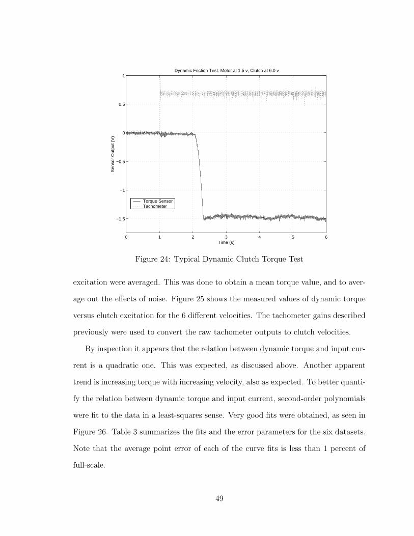
0 1 2 3 4 5 6

−1.5

−1

−0.5

0

0.5

1Dynamic Friction Test: Motor at 1.5 v, Clutch at 6.0 v

Time (s)

Sen

sor

Out

put (

V)

Torque SensorTachometer

Figure 24: Typical Dynamic Clutch Torque Test

excitation were averaged. This was done to obtain a mean torque value, and to aver-

age out the effects of noise. Figure 25 shows the measured values of dynamic torque

versus clutch excitation for the 6 different velocities. The tachometer gains described

previously were used to convert the raw tachometer outputs to clutch velocities.

By inspection it appears that the relation between dynamic torque and input cur-

rent is a quadratic one. This was expected, as discussed above. Another apparent

trend is increasing torque with increasing velocity, also as expected. To better quanti-

fy the relation between dynamic torque and input current, second-order polynomials

were fit to the data in a least-squares sense. Very good fits were obtained, as seen in

Figure 26. Table 3 summarizes the fits and the error parameters for the six datasets.

Note that the average point error of each of the curve fits is less than 1 percent of

full-scale.

49

0 1 2 3 4 5 6 7 8 9 100

100

200

300

400

500

600

700

800Dynamic Clutch Torque

Clutch Excitation Command (V)

Tor

que

(lb−

in)

0.194 rad/s0.394 rad/s0.792 rad/s1.193 rad/s1.591 rad/s1.990 rad/s

Figure 25: Measured Dynamic Clutch Torque

0 1 2 3 4 5 6 7 8 9 100

100

200

300

400

500

600

700

800Dynamic Torque Data with Individual Quadratic Fits


Tor

que

(lb−

in)

0.194 rad/sec0.394 rad/sec0.792 rad/sec1.193 rad/sec1.591 rad/sec1.990 rad/sec

Figure 26: Measured Dynamic Clutch Torque with Individual Quadratic Fits

50

These curve fits provide a good model which represents the experimental data, but

are not very useful in their present state for use in the simulation. The fits represent

models continuous in clutch excitation, but for only six discrete clutch velocities. A

model for dynamic torque which is continuous in both clutch excitation and clutch

velocity is desired. To this end, it was decided to select one of the above fits and

multiply it by a scaling factor which is dependent on clutch velocity.

The base quadratic that was selected was that of the 0.394rads case. This is the

only example out of the six fits that exhibits two important physical characteristics

required by a good dynamic torque model. First, it has a positive y-intercept, and

second, it has positive slope at all positive clutch excitation commands. The former

condition is dictated by the clutches’ passivity constraints, and the latter by physical

insight— the clutches should at no time create a lower amount of torque corresponding

to an increased current input.

Different scaling factors were tried for each of the other velocities, and least-squares

error was again used to select the best term. A linear equation was then fit to these

scaling factors in order to obtain a continuous model of scaling factor versus clutch

velocity. Finally, the model of clutch dynamic torque continuous in both excitation

(v) and velocity (ω) is as follows:

Motor Speed Average Error

( rads

) Fit Equation∑

e2 per point (lb-in)

0.194 6.060v2− 0.193v + 1.496 1018 4.98

0.394 6.439v2 + 0.137v + 0.371 1219 5.45

0.792 6.834v2 + 2.167v − 1.102 889.9 4.66

1.193 7.158v2 + 3.143v − 2.405 984.8 4.90

1.591 6.954v2 + 5.445v − 3.899 1005 4.95

1.990 7.462v2 + 4.312v − 2.711 871.8 4.61

Table 3: Individual Quadratic Fits and Error Parameters

51

0 1 2 3 4 5 6 7 8 9 100

100

200

300

400

500

600

700

800

900Dynamic Torque Data with Scaled Quadratic Fit


Tor

que

(lb−

in)

0.194 rad/sec0.394 rad/sec0.792 rad/sec1.193 rad/sec1.591 rad/sec1.990 rad/sec

Figure 27: Measured Dynamic Clutch Torque with Single Scaled Quadratic Fit

τdyn = (0.154ω + 0.9409)(6.439v2 + 0.137v + 0.371) (39)

Figure 27 is a plot of the scaled polynomial fit and the experimental data. Figure

28 is a surface plot of of the final model. Error parameters are summarized in Table

4. Even though the average error values of the scaled fit are higher than those of the

individual fits, they are still low— within 2 percent of full-scale.

Motor Speed Average Error

( rads

)∑

e2 per point (lb-in)

0.194 4907 10.93

0.394 1230 5.48

0.792 4924 10.96

1.193 6047 12.14

1.591 3153 8.77

1.990 2792 8.25

Table 4: Scaled Quadratic Fit and Error Parameters

52

0 2 4 6 8 10

00.5

11.5

22.5

0

100

200

300

400

500

600

700

800

900

Clutch Excitation Voltage (V)

Final Clutch Dynamic Torque Model

Clutch Velocity (rad/s)

Tor

que

(in−

lbs)

Figure 28: Final Dynamic Clutch Torque Model

4.6.2.2 Breakaway Torque

The second friction phenomena that was to be modeled was the breakaway torque,

which corresponds to the maximum static friction that the clutch can produce. Sev-

eral tests were done to model this phenomena. In these tests, the servomotor was set

on torque control. A constant input current was applied to the clutch, and a ramped

torque was commanded to the motor. Figure 29 is a plot of a typical breakaway test

run. This test represents an excitation command of 7 volts to the clutch. The torque

sensor measures a ramped torque input, as was commanded to the motor, up until the

clutch starts to slip. This occurs at approximately 2.9 seconds, where the tachometer

output starts to increase from zero. There is a drop in friction at this point, charac-

teristic of the fact that static friction is typically higher than dynamic friction. The

torque level quickly increases after the momentary post-transition decrease due to

the increasing velocity of the motor. As seen in the above section, dynamic torque

increases with higher velocity. Since the servomotor is set to torque control, it ramps

up the speed of the clutch plate in order to achieve the higher required torques after

53

0 0.5 1 1.5 2 2.5 3 3.5 4−4

−2

0

2

4

6

8Breakaway Torque Test Data − 7 volt Clutch Input

Time (s)

Sen

sor

Out

put (

V)


Figure 29: Typical Breakaway Torque Test Data

slip occurs.

Figure 30 is a detail of Figure 29. This shows more closely the behavior of the

system at the breakaway point. An oscillation at the breakaway point of about 90

Hz is present in the torque signal. This vibration is likely caused by the compliance

of the torque sensor. The torque sensor and clutch coil can be thought of as a mass

on a massless torsional spring. The mass of the coil is approximately 45 times that

of the torque sensor, so the massless assumption should be valid.

The torque sensor can be approximately modeled as a 2 inch long aluminum

cylinder of 1 132

inch diameter. Its torsional stiffness kτ is then

kτ =GIp

L=

(26E109 Nm)π(0.0273 m)4

32(0.0508 m)= 27910 N · m (40)

where G is the shear modulus of aluminum, Ip is the polar moment of inertia of

54

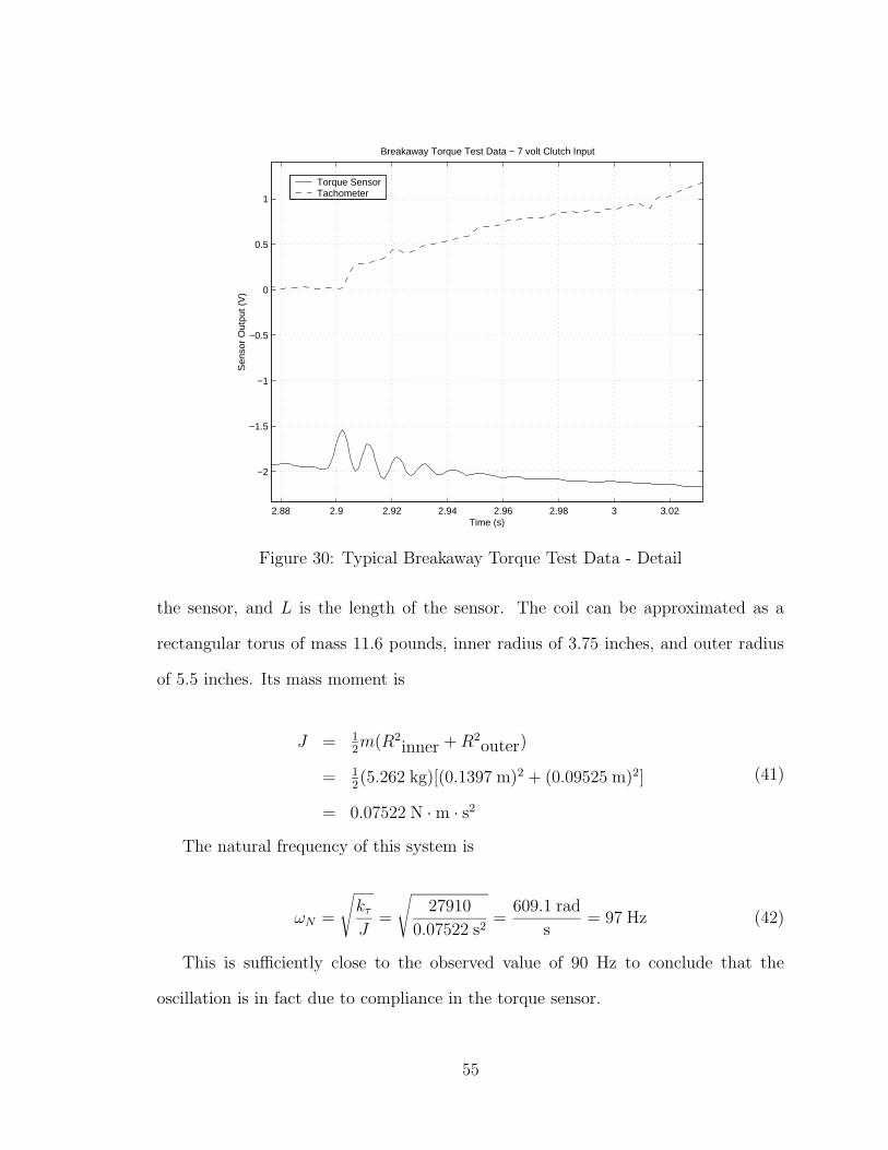
2.88 2.9 2.92 2.94 2.96 2.98 3 3.02

−2

−1.5

−1

−0.5

0

0.5

1

Breakaway Torque Test Data − 7 volt Clutch Input

Time (s)

Sen

sor

Out

put (

V)


Figure 30: Typical Breakaway Torque Test Data - Detail

the sensor, and L is the length of the sensor. The coil can be approximated as a

rectangular torus of mass 11.6 pounds, inner radius of 3.75 inches, and outer radius

of 5.5 inches. Its mass moment is

J = 12m(R2

inner + R2outer)

= 12(5.262 kg)[(0.1397 m)2 + (0.09525 m)2]

= 0.07522 N · m · s2

(41)

The natural frequency of this system is

ωN =

√

kτ

J=

√

27910

0.07522 s2=

609.1 rad

s= 97 Hz (42)

This is sufficiently close to the observed value of 90 Hz to conclude that the

oscillation is in fact due to compliance in the torque sensor.

55

0 1 2 3 4 5 6 7 8 9 100

100

200

300

400

500

600

700

800Measured Breakaway Torque Levels

Clutch Command Input (V)

Tor

que

(in−

lbs)

Figure 31: Breakaway Torques

Data was taken at 41 different clutch excitation commands, from zero to 10 volts at

0.25 volt steps. The datasets were examined, and the highest torque value measured

prior to clutch slip was chosen to be the breakaway torque level. Figure 31 shows

the breakaway torque levels for all datasets. Torques were not determined for clutch

commands below 2.25 volts, as the noise in the data did not allow determination of

the breakaway level. Immediately, one may notice that the data is not as clean as the

data for the dynamic tests. This could be due to several factors, among which are the

torque profile provided by the motor to the clutch during the test and compliance in

the testbed. The data, however, is still usable. Theoretically the breakaway torque

level should be proportional to the clutch plate normal force, and hence to the square

of the input current, as discussed above. Fitting a least-squares quadratic

56

τbrk = 6.648v2 + 6.176v + 5.253 (43)

to the breakaway torque does a satisfactory job of representing the trend of the

data (see Figure 32). When compared to the dynamic friction model at low speed

(see Figure 33), it is seen that the breakaway torque curve remains above dynamic

torque at all times, and even resembles the shape of the dynamic torque curve. This

makes sense— both torques are dependent on the clutch plate normal force, which

is constant at steady-state for a given clutch excitation voltage. The only difference

between the two curves lies in the different friction phenomena involved— static and

dynamic.

4.7 Comparison - Torque Bar Tests and Motorized

Testbed Tests

There now exist two separate sets of experimental data and associated models for the

clutches. The first was derived from the torque bar tests and the second from the

motorized testbed tests, both of which were explained previously in this chapter.

Figure 34 compares the static and dynamic torque models built from each set of

tests. The motorized testbed tests clearly recorded a higher torque level than the

torque bar tests. This could be due to the fact that the clutch response is partially

dependent on mounting. The preloading of the spring element that supports the

floating clutch plate will affect the normal force and as a result the available torque.

This could also be due to the instrumentation involved. The testbed tests used a

calibrated commercial torque sensor, and the torque bar tests used a torque sensor

prototyped in the lab. This would lead one to believe that the testbed tests provide

57

0 1 2 3 4 5 6 7 8 9 100

100

200

300

400

500

600

700

800Measured Breakaway Torque Levels and Quadratic Fit


Tor

que

(in−

lbs)

Measured ValuesQuadratic Fit

Figure 32: Measured Breakaway Torques with Quadratic Fit

0 1 2 3 4 5 6 7 8 9 100

100

200

300

400

500

600

700

800Model Comparison − Breakaway and Dynamic Torque


Tor

que

(in−

lbs)

Breakaway Torque Model Dynamic Torque Model − 0.194 rad/s

Figure 33: Dynamic and Breakaway Torque Model Comparison

58

0 1 2 3 4 5 6 7 8 9 100

100

200

300

400

500

600

700

800

Clutch Excitation Voltage (V)

Tor

que

(in−

lbs)

Model Comparison − Testbed Tests and Torque−bar Tests

Testbed model − Breakaway Torque Testbed model − Dynamic Torque (0.194 rad/s)Torque−Bar model − Breakaway Torque Torque−Bar model − Dynamic Torque

Figure 34: Model Comparison of the Two Clutch Tests

a more accurate measure of the generated clutch torques. That they are higher than

previously thought is not surprising— the stock clutches are capable of producing

well over 1000 lb-in of torque.

The models built from the testbed data should also be more accurate since points

were taken at 41 different values of clutch excitation voltage, as opposed to 6 in the

torque bar tests. Also, the torque bar tests did not consider velocity at all in the

modeling of dynamic torque.

59

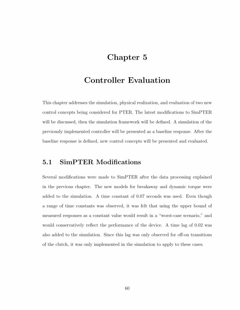
Chapter 5

Controller Evaluation

This chapter addresses the simulation, physical realization, and evaluation of two new

control concepts being considered for PTER. The latest modifications to SimPTER

will be discussed, then the simulation framework will be defined. A simulation of the

previously implemented controller will be presented as a baseline response. After the

baseline response is defined, new control concepts will be presented and evaluated.

5.1 SimPTER Modifications

Several modifications were made to SimPTER after the data processing explained

in the previous chapter. The new models for breakaway and dynamic torque were

added to the simulation. A time constant of 0.07 seconds was used. Even though

a range of time constants was observed, it was felt that using the upper bound of

measured responses as a constant value would result in a “worst-case scenario,” and

would conservatively reflect the performance of the device. A time lag of 0.02 was

also added to the simulation. Since this lag was only observed for off-on transitions

of the clutch, it was only implemented in the simulation to apply to these cases.

60

5.2 Simulation Framework

5.2.1 Definition of Simulation Runs

It is necessary to define a standard simulation run in order to compare different

control concepts. The test used exclusively in this chapter is a line-following test.

The controller attempts to constrain the tip of the device to a straight line in its

workspace. The tip of the robot is initially located on the line. The simulated user

applies force to the tip. One component of this force is constant parallel to the

desired path. There is also a disturbance component normal to the desired path,

which consists of a sum of several sinusoids of different frequencies. Several factors

went into choosing this disturbance signal. A white or Gaussian noise input would

not be appropriate due to the fact that this is a physical system, and such an input

consists of sufficiently high frequencies that it would not have much of an effect on

the output of the device, and would in any case be a bad representation of the forces

that an actual user would input to the tip of the robot. A sinewave input would allow

for enough lateral force in a single direction to cause significant movement in the

tip. It is also repeatable between simulation run, allowing for direct comparison of

system response. A single sinewave at a single frequency, however, is still not a good

representation of actual input. It has been observed that a sinewave of the proper

frequency may interact with the system’s dynamics and cause conditions where the

controller does not allow the tip to move at all. In this light, it was desired that a

richer input signal consisting of several frequencies would be appropriate.

Simulation runs are terminated based on a distance constraint in the workspace.

The desired path lies along the y-axis of the workspace, and the tip moves from right

to left. A constant-x line is defined as the limit of travel. Once the tip of the robot

61

ActualTip Path

Desired Tip Path

(x1,y1,t1)

(x2,y2,t2)(x3,y3,t3)

(x4,y4,t4)e1

e2

e3

e4

x

y

Figure 35: Tracking Error Definition

moves left of this stopping point, the simulation is halted.

5.2.2 Measures of System Performance

After a standard test was defined, it was necessary to define the measures by which we

would compare the different control schemes. The primary goal of PTER’s controller

in this work is position tracking. A secondary goal is the hard-to-quantify concept of

“feel”. Feel in this case is associated with the smoothness of operation of the device.

Position tracking performance is measured by a weighted average position error.

See Figure 35. At each sampling instant (xk, yk, tk in the Figure), the position error

(ek) is defined as the distance between the current tip position and the closest point on

the desired path. This distance is weighted by half the actual path distance between

the previous and next sampling instants. For example, the weighted position error p

at point 2 in the figure would be:

p2 =

√

(x3 − x2)2 + (y3 − y2)2 +√

(x2 − x1)2 + (y2 − y1)2

2

e2 (44)

These errors are summed over all data points and divided by the total actual

path length. This results in an error term that may be compared between different

simulation runs that have necessarily different actual path profiles. This position

62

error is used to quantify position tracking performance.

With regard to feel, or smoothness, two performance measures are used. The time

derivative of the linear acceleration of the tip of the robot is one measure. This value

is commonly referred to as the “jerk”, and is a measure of the time rate of change

of force applied to the tip of the robot. Unfortunately, in reality jerk is difficult to

measure, so linear acceleration is also used as a performance measure which may be

compared with measured data. Weighted averages of jerk and acceleration is taken

similar to the process used in calculating position error as described above, but instead

of weighting the terms with path length, they are weighted with time. So, if jk is the

linear jerk of the tip and ak is the linear acceleration of the tip, both at time k, the

weighted terms j and a at point 2 would be:

a2 =(

t3 − t1

2

)

a2 (45)

j2 =(

t3 − t1

2

)

j2 (46)

The errors are summed over all data points and divided by the total simulation

time to obtain time-weighted average jerk and acceleration.

5.3 Baseline Controller

5.3.1 Controller Definition

The baseline controller consists of the impedance controller and torque translator

described in the previous section. This controller has already been implemented and

demonstrated on the physical hardware. It is in fact the only controller to have been

implemented in simulation up to this point. These factors make it a good candidate

63

Selector Torque

Controller Clutchτ des

Command Voltages

PTERState

PTER Controller

Figure 36: Division of PTER’s Controller

for the baseline controller.

At this point, it is helpful to recall that an arbitrary PTER controller may be

divided into two conceptual halves. See Figure 36. The torque selector determines an

achievable (i.e., not violating the passivity constraint) desired set of clutch torques

based on the current system state and the desired path. This set of desired torques

is passed on to a clutch controller, which determines excitation voltages to be sent to

the clutches.

The impedance controller and torque translator in use by the baseline controller

represents only the torque selector portion of the overall controller. It merely deter-

mines a set of desired clutch torques. The clutch controller is simply a look-up table

based on a previous model of the clutch torque response. It is important to note that

this look-up table does not match the models computed in the previous chapter and

used by the clutch model in the simulation.

5.3.2 Simulated Results

A baseline run was performed. The desired path was the line y = 24 in the workspace.

The origin of the workspace is defined as the main axis of PTER— the axis running

through the center of all four clutches. The tip of the robot is initially located at

(3, 24), on the desired path. The constant tangent component of the input force is 7

lb and the magnitude of the sinusoidal normal component is 5 lb.

64

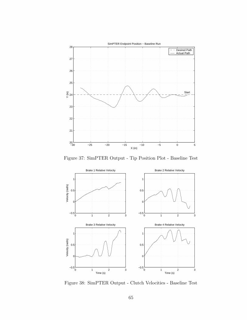
−30 −25 −20 −15 −10 −5 0 520

21

22

23

24

25

26

27

28

X (in)

Y (

in)

SimPTER Endpoint Position − Baseline Run

Start

Desired PathActual Path

Figure 37: SimPTER Output - Tip Position Plot - Baseline Test

0 1 2 3−0.5

0

0.5

1

Brake 1 Relative Velocity

Vel

ocity

(ra

d/s)

0 1 2 3−0.5

0

0.5

1


0 1 2 3−0.5

0

0.5

1


Vel

ocity

(ra

d/s)

Time (s)0 1 2 3

−0.5

0

0.5

1


Time (s)

Figure 38: SimPTER Output - Clutch Velocities - Baseline Test

65

Figure 37 is a plot of the simulated tip position for the baseline test. Notice

that the scale of the plot is not equal in both axes. The y-axis has been magnified

to better illustrate the off-path behavior of the tip. Figure 38 is a diagram of the

relative clutch plate velocities of all four clutches for the baseline run. In these plots,

one can easily see the action of the friction model— when a clutch velocity reaches

zero, it sticks for a finite period of time. The velocity remains zero until the applied

torque is high enough to cause it to slip. The result is a flat portion of the velocity

graph along the x-axis. This occurs twice for clutch 2 and four times for clutch 4 in

Figure 38. Notice in Figure 39 that the instantaneous magnitude of the jerk at the

tip of the robot peaks whenever one of the clutches makes a stick-slip transition. This

is similar to what happens on the physical testbed, a very jerky feeling when stiction

effects occur, and shows that the newly implemented friction model does a good job

of representing the effect of friction on device feel.

Figure 40 is a comparison of linear tip jerk and linear tip acceleration magnitudes.

It is seen from this plot that areas of high jerk can be identified by locating high

gradients on a plot of acceleration versus time. Therefore, experimental acceleration

data can be helpful in identifying instants of high jerk in the absence of actual jerk

data.

5.4 Proportional Torque Control


The first new control concept was that of proportional torque feedback control. This

controller makes use of the same controller as used in the baseline case, but adds

proportional feedback to the clutch controller portion. Figure 41 is a block diagram

66

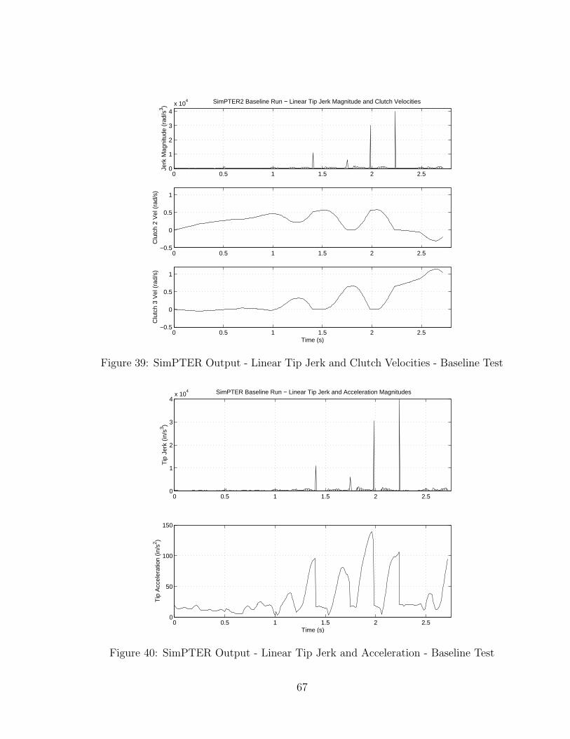
0 0.5 1 1.5 2 2.50

1

2

3

4x 10

4

Jerk

Mag

nitu

de (

rad/

s3 )

SimPTER2 Baseline Run − Linear Tip Jerk Magnitude and Clutch Velocities

0 0.5 1 1.5 2 2.5−0.5

0

0.5

1

Clu

tch

2 V

el (

rad/

s)

0 0.5 1 1.5 2 2.5−0.5

0

0.5

1

Time (s)

Clu

tch

3 V

el (

rad/

s)

Figure 39: SimPTER Output - Linear Tip Jerk and Clutch Velocities - Baseline Test

0 0.5 1 1.5 2 2.50

1

2

3

4x 10

4

Tip

Jer

k (in

/s3 )

SimPTER Baseline Run − Linear Tip Jerk and Acceleration Magnitudes

0 0.5 1 1.5 2 2.50

50

100

150

Time (s)

Tip

Acc

eler

atio

n (in

/s2 )

Figure 40: SimPTER Output - Linear Tip Jerk and Acceleration - Baseline Test

67

Selector Torque

PTERState τ des v τ act

K

ClutchesLook-Up Table

v

-

+

+

+

Figure 41: Clutch Controller with Proportional Torque Feedback

2

DesiredTorques

1

Voltages (4)

−K−

Torque_Gain_4

−K−

Torque_Gain_3

−K−

Torque_Gain_2

−K−

Torque_Gain_1

Saturation

Mux

Mux1

Mux

Mux

MATLABFunction

ImpedanceController

Error 4

Error 3

Error 2

Error 1

Control 4

Control 3

Control 1

Control 2Demux

Commands andDesired Torques

|u|

Abs3

|u|

Abs2

|u|

Abs1

|u|

Abs

Trigger

5

Clutch 4Actual Torque

4


3


2


1

InputVector

Figure 42: Clutch Controller with Proportional Torque Feedback - SimPTER Imple-mentation

of the modified clutch controller. Notice that the same look-up table is used, but

a proportional error term is added to its output. This serves to compensate for

modeling errors within the look-up table. Figure 42 shows the implementation of this

controller within SimPTER.

In PTER’s current configuration, this controller is not realizable, since there is

no way to obtain the required torque feedback from each clutch. Another project is

currently underway to design a modification that would add an integrated, colocated

torque sensor to each clutch. If PTER’s clutches were modified in this manner, it

would be possible to implement a torque feedback controller.

68


To determine the effect of the proportional gain of this controller on system perfor-

mance, a sequence of simulations were run at different gain values. The set of four

gains (one for each clutch) were equal in each run. The two system performance

parameters, position error and linear jerk magnitude, were examined for each run.

Figures 43 and 44 are plots of average position error and average linear jerk over

several different values of controller gain. Notice that the proportional action de-

creases both error measures, resulting in an increased level of performance, up to a

certain point, and then affects them in a seemingly random fashion. This is due to

the fact that over gains of approximately 0.2, significant levels of actuator saturation

are present.

A controller gain of 0.16 was selected for the remainder of the simulation analy-

sis. This gain was picked because it represented a good measure of improvement in

both position error and smoothness. Although the position error appears to follow

a downward trend with values of gain higher than 0.16, the average jerk increases

considerably. This behavior is not surprising. Higher gains will in general lead to

higher control action. This can eventually lead to oscillation and high rates of change

of commanded clutch torques, increasing the average value of linear jerk. A gain of

0.16 was considered a good tradeoff between the two performance measures.

Figure 45 is a plot of the simulated endpoint position of both the baseline controller

and the proportional torque feedback controller with a gain of 0.16. The improvement

in position tracking performance is apparent from this graph. The effect of the new

controller on several system variables is summarized in Table 5. It can be seen from

the table that the linear jerk and acceleration parameters have also decreased.

It is apparent that, according to the simulation, proportional torque feedback can

69

0 0.1 0.2 0.3 0.4 0.5 0.60

0.05

0.1

0.15

0.2

0.25

0.3

0.35

0.4Average Position Error vs Proportional Control Gain

Gain

Err

or (

in)

Figure 43: Proportional Torque Feedback Controller - Position Tracking Performance

0 0.1 0.2 0.3 0.4 0.5 0.6300

350

400

450

500

550

600Average Linear Jerk vs Proportional Control Gain

Gain

Jerk

(in

/s3 )

Figure 44: Proportional Torque Feedback Controller - Smoothness Measure

70

−30 −25 −20 −15 −10 −5 0 520

21

22

23

24

25

26

27

28

X (in)

Y (

in) Start

Baseline and Proportional Torque Control Comparison − SimPTER Endpoint Position

Desired Path Baseline with P Torque Control (gain=0.16)

Figure 45: Endpoint Position - Baseline and Proportional Torque Feedback Controller

improve the performance of PTER. However, two questions arise. First of all, why

does it improve performance? Secondly, why would it decrease levels of jerk, as well

as decreasing the average position error?

The answer to the first question is well illustrated by Figures 46 and 47. These

figures show the desired torques computed by the controller for clutch 2 and the

actual torques generated by the clutch model. The actual generated torque does not

exactly match the desired in either case due to the modeled system dynamics and

the fact that the models used in the controller look-up table and in the clutch model

Average Pos Max Pos Average Lin Max Lin Total Path Average Lin Max Lin

Controller Error (in) Error (in) Jerk ( in

s3) Jerk ( in

s3) Length (in) Accel ( in

s2) Accel ( in

s2)

Baseline 0.360 1.078 456 40118 32.205 31.53 139.8P Feedback(gain=0.16) 0.132 0.299 317 3501 31.154 17.58 79.69

Table 5: Simulation Results of Baseline and Torque Feedback Controllers

71

0 0.5 1 1.5 2 2.50

100

200

300

400

500

600

Time (s)

Tor

que

(lb−

in)

Actual and Desired Clutch 2 Torques − Baseline Controller

Actual Torque Desired Torque

Figure 46: Clutch 2 Torque Following - Baseline Controller

0 0.5 1 1.5 2 2.50

100

200

300

400

500

600

Time (s)

Tor

que

(lb−

in)

Actual and Desired Clutch 2 Torques − P Torque Feedback Controller

Actual Torque Desired Torque

Figure 47: Clutch 2 Torque Following - P Feedback Controller (Gain=0.16)

72

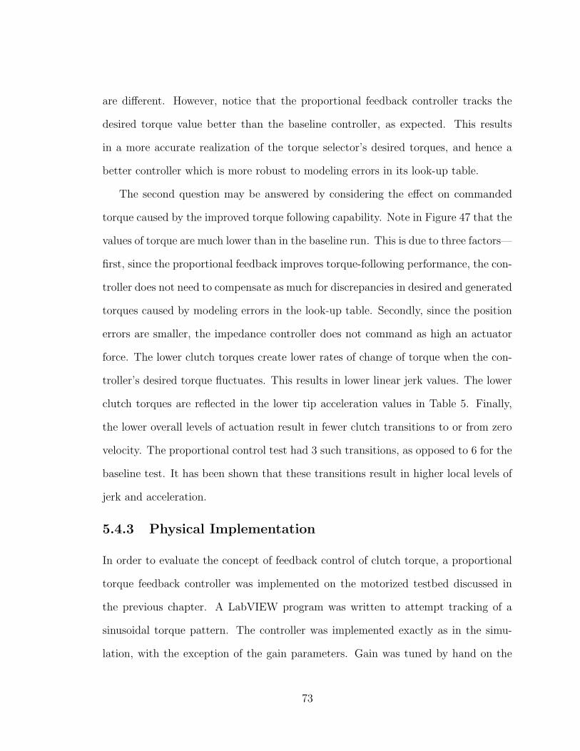
are different. However, notice that the proportional feedback controller tracks the

desired torque value better than the baseline controller, as expected. This results

in a more accurate realization of the torque selector’s desired torques, and hence a

better controller which is more robust to modeling errors in its look-up table.

The second question may be answered by considering the effect on commanded

torque caused by the improved torque following capability. Note in Figure 47 that the

values of torque are much lower than in the baseline run. This is due to three factors—

first, since the proportional feedback improves torque-following performance, the con-

troller does not need to compensate as much for discrepancies in desired and generated

torques caused by modeling errors in the look-up table. Secondly, since the position

errors are smaller, the impedance controller does not command as high an actuator

force. The lower clutch torques create lower rates of change of torque when the con-

troller’s desired torque fluctuates. This results in lower linear jerk values. The lower

clutch torques are reflected in the lower tip acceleration values in Table 5. Finally,

the lower overall levels of actuation result in fewer clutch transitions to or from zero

velocity. The proportional control test had 3 such transitions, as opposed to 6 for the

baseline test. It has been shown that these transitions result in higher local levels of

jerk and acceleration.

5.4.3 Physical Implementation

In order to evaluate the concept of feedback control of clutch torque, a proportional

torque feedback controller was implemented on the motorized testbed discussed in

the previous chapter. A LabVIEW program was written to attempt tracking of a

sinusoidal torque pattern. The controller was implemented exactly as in the simu-

lation, with the exception of the gain parameters. Gain was tuned by hand on the

73

0 1 2 3 4 5 6 7 80

50

100

150

200

250Testbed Comparison of LUT and LUT+P Feedback Control

Time (s)

Tor

que

(lb−

in)

Response with P control Response without P controlDesired Response

Figure 48: Implemented Torque Controller - With and Without P Feedback

testbed until a satisfactory response was achieved.

Figure 48 is a comparison of the tracking performances of the look-up table con-

troller and the same controller with proportional feedback. In this case, the propor-

tional feedback gain is 0.08. Although it does not give perfect tracking performance,

it can be seen that the proportional feedback does decrease the tracking error.

Some initial oscillation can be observed in the feedback controller due to the nonze-

ro desired initial condition and resulting high initial error present when the controller

starts. Higher gains were attempted in order to further decrease the tracking error,

but the system quickly experienced high oscillations. Figure 49 is a plot of the track-

ing performance of the feedback controller at a gain of 0.20. The unstable oscillation

is apparent.

It is proposed that the high level oscillations are due to the fact that the controller

74

0 1 2 3 4 5 6 7 80

50

100

150

200

250

300

350

Time (s)

Tor

que

(lb−

in)

Proportional Feedback Controller − Gain = 0.20

Figure 49: Implemented Proportional Feedback Controller (gain=0.20) - UnstableBehavior

is discrete and is running at a relatively low frequency, and are not due to stick-slip

or stiction effects within the clutch. To determine whether or not this is the case,

SimPTER was slightly modified to apply a constant input torque to a single clutch

and have the controller attempt to regulate the clutch torque to a constant level. This

is similar to the configuration of the testbed. 250 lb-in was input into clutch 1, and

the proportional feedback controller was configured to regulate the generated torque

at 150 lb-in. Four simulations were run. In the first three, the controller ran at 30

Hz (the same as the testbed controller) for gains of 0 (no P control action), 0.08, and

0.25. The controller ran at 150 Hz with a gain of 0.25 in the fourth simulation. Figure

50 shows generated clutch torque for each of the four tests. The zero gain condition

is included as a reference with no feedback control action. A gain of 0.08 shows a

regulated torque with an error of approximately 20 lb-in. The 0.20 gain condition

75

0 0.1 0.2 0.3 0.4 0.50

50

100

150

200

250

Tor

que

(lb−

in)

Controller: 30 Hz, Gain=0

0 0.1 0.2 0.3 0.4 0.50

50

100

150

200

250Controller: 30 Hz, Gain=0.08

0 0.1 0.2 0.3 0.4 0.50

50

100

150

200


Time (s)0 0.1 0.2 0.3 0.4 0.5

0

50

100

150

200


Time (s)

Figure 50: Simulation of Testbed Torque Feedback Controller

experiences oscillations similar to those seen on the testbed above. Keeping the gain

at 0.20 and increasing the controller speed fivefold to 150 Hz stabilizes the controller

and eliminates the oscillation. In this case the steady-state error is less than 10 in-lbs.

These simulations lend weight to the argument that the oscillations in the testbed

feedback controller are caused by a gain that is too high for the discretized controller.

Increasing the update rate of the testbed controller should allow higher gains and

reduced tracking error without oscillation.

5.5 Velocity Controller


The velocity based controller was first suggested by Gomes. [11] This controller

functions in the capacity of a torque selector— it provides a desired set of clutch

76

DesiredVelocity

DesiredVelocity

��

��

Desired Path

Possible Tip Positions

Tip VelocityTip Velocity

Figure 51: Desired Velocity Determination - Implemented Gomes Velocity Controller

DesiredVelocity

��

��

��

Desired Path

Tip Velocity

Possible Tip Positions

Figure 52: Desired Velocity Determination - Proposed Velocity Controller

torques based on the system state. It was implemented by Gomes on PTER in a basic

form and showed promise as a improved alternative to the impedance controller.

While the impedance controller attempts to control the tip based on position error

through the modeling of spring and damper elements between the tip of the robot

and the desired path, the velocity controller attempts to guide the linear tip velocity

towards a certain direction. Gomes defined a simple desired velocity vector— it has a

desired path-tangent component in the same direction as the current tip velocity, and

a desired path-normal component of the same magnitude towards the desired path.

This yields vectors at 45 degree angles to a straight line desired path, as shown in

Figure 51.

For the current implementation of the velocity controller, the determination of

77

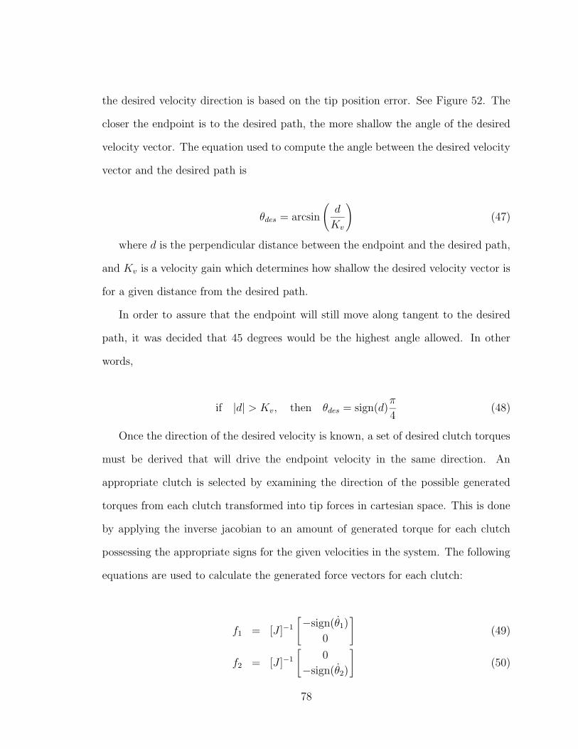
the desired velocity direction is based on the tip position error. See Figure 52. The

closer the endpoint is to the desired path, the more shallow the angle of the desired

velocity vector. The equation used to compute the angle between the desired velocity

vector and the desired path is

θdes = arcsin

(

d

Kv

)

(47)

where d is the perpendicular distance between the endpoint and the desired path,

and Kv is a velocity gain which determines how shallow the desired velocity vector is

for a given distance from the desired path.

In order to assure that the endpoint will still move along tangent to the desired

path, it was decided that 45 degrees would be the highest angle allowed. In other

words,

if |d| > Kv, then θdes = sign(d)π

4(48)

Once the direction of the desired velocity is known, a set of desired clutch torques

must be derived that will drive the endpoint velocity in the same direction. An

appropriate clutch is selected by examining the direction of the possible generated

torques from each clutch transformed into tip forces in cartesian space. This is done

by applying the inverse jacobian to an amount of generated torque for each clutch

possessing the appropriate signs for the given velocities in the system. The following

equations are used to calculate the generated force vectors for each clutch:

f1 = [J ]−1

[

−sign(θ1)

0

]

(49)

f2 = [J ]−1

[

0

−sign(θ2)

]

(50)

78

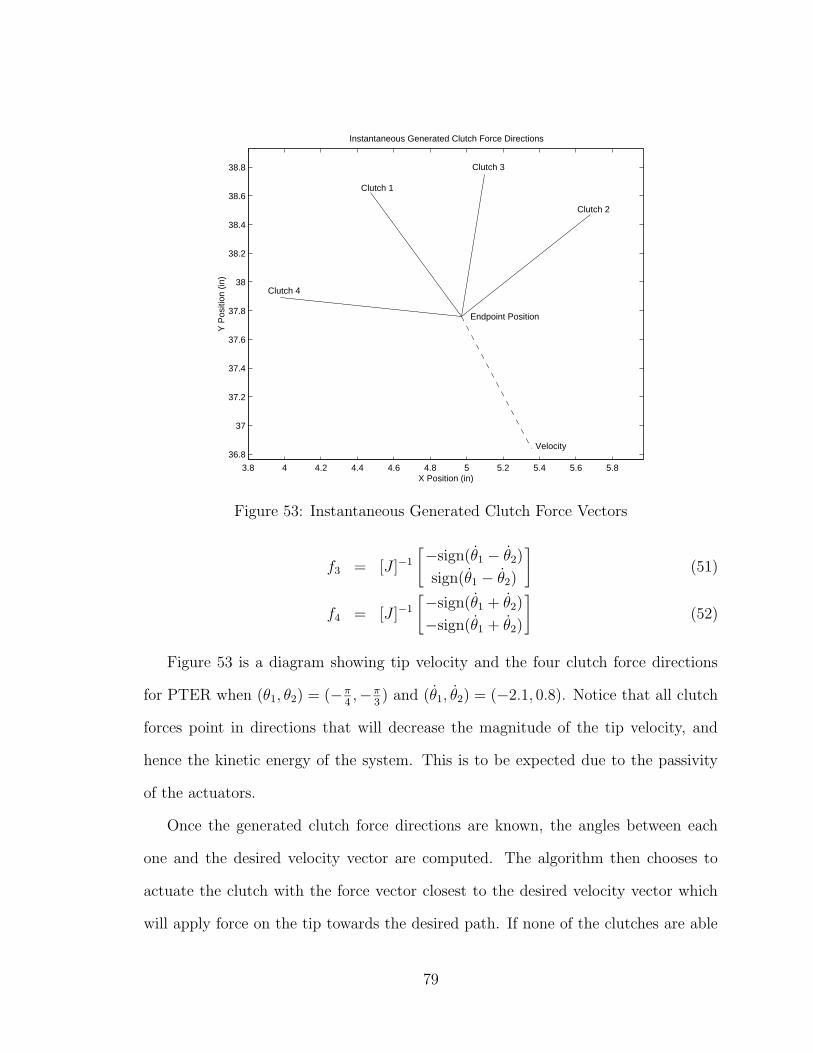
3.8 4 4.2 4.4 4.6 4.8 5 5.2 5.4 5.6 5.8

36.8

37

37.2

37.4

37.6

37.8

38

38.2

38.4

38.6

38.8

Velocity

Endpoint Position

Clutch 1

Clutch 2

Clutch 3

Clutch 4

X Position (in)

Y P

ositi

on (

in)

Instantaneous Generated Clutch Force Directions

Figure 53: Instantaneous Generated Clutch Force Vectors

f3 = [J ]−1

[

−sign(θ1 − θ2)

sign(θ1 − θ2)

]

(51)

f4 = [J ]−1

[

−sign(θ1 + θ2)

−sign(θ1 + θ2)

]

(52)

Figure 53 is a diagram showing tip velocity and the four clutch force directions

for PTER when (θ1, θ2) = (−π4,−π

3) and (θ1, θ2) = (−2.1, 0.8). Notice that all clutch

forces point in directions that will decrease the magnitude of the tip velocity, and

hence the kinetic energy of the system. This is to be expected due to the passivity

of the actuators.

Once the generated clutch force directions are known, the angles between each

one and the desired velocity vector are computed. The algorithm then chooses to

actuate the clutch with the force vector closest to the desired velocity vector which

will apply force on the tip towards the desired path. If none of the clutches are able

79

to push the tip back towards the desired path, the controller will act in one of two

ways. If the user applied tip force points away from the desired path, it will apply

full voltage to two clutches in order to completely lock the system. Otherwise, it will

release all clutches to allow the user applied force to push the tip back towards the

desired path.

If the controller identifies a satisfactory clutch and decides to actuate it, the ac-

tuation magnitude is determined based on the relative angle between the current tip

velocity vector and the desired velocity vector. This angle is multiplied by the actu-

ated clutch’s force component normal to the desired path and by a gain to calculate

a desired torque magnitude as follows:

|τ | = KτfN |θvdes − θv| (53)


The velocity controller was implemented in combination with the proportional torque

feedback controller described in the previous section. The improved torque following

abilities of the feedback controller have already been shown, and since the effectiveness

of the velocity controller is dependent on the magnitudes of the actuation torques it

was thought that better performance could be achieved by combining the two. The

two controllers are independent. The velocity controller makes up the torque selector

part of the PTER controller, and the proportional feedback controller affects the

clutch controller portion.

The simulation was run with a Kv value of 1. Figure 54 is an endpoint comparison

plot of the original impedance controller and the new velocity controller, both with

proportional torque feedback. Feedback gains of 0.16 were used for both runs. It is

80

−30 −25 −20 −15 −10 −5 0 520

21

22

23

24

25

26

27

28

X (in)

Y (

in)

Endpoint Path − Baseline Controller and Velocity Controller (both with P feedback)

Desired Path Baseline (Impedance) ControllerVelocity Controller

Figure 54: Impedance and Velocity Controller Comparison - Endpoint Position

apparent from the Figure that the velocity controller does a better job of following

the desired path. Table 6 lists some error parameters for all three controllers.

The linear jerk values illustrate that although the velocity controller exhibits in-

creased path following performance, it is less smooth than the impedance controller

with torque feedback. On the other hand, the linear acceleration parameters of the

velocity controller are lower than those of the other two. Figure 55 is a comparison of

Avg Pos Max Pos Avg Lin Max Lin Total Path Avg Lin Max Lin

Controller Error (in) Error (in) Jerk ( in

s3) Jerk ( in

s3Length (in) Accel ( in

s2) Accel ( in

s2)

Baseline(ImpedanceController) 0.360 1.078 456 40118 32.205 31.53 139.8Impedance w/P Feedback(gain=0.16) 0.132 0.299 317 3501 31.154 17.58 79.69Velocity w/P Feedback(gain=0.16) 0.067 0.161 439 49774 31.034 15.77 42.18

Table 6: Simulation Results of Several Controllers

81

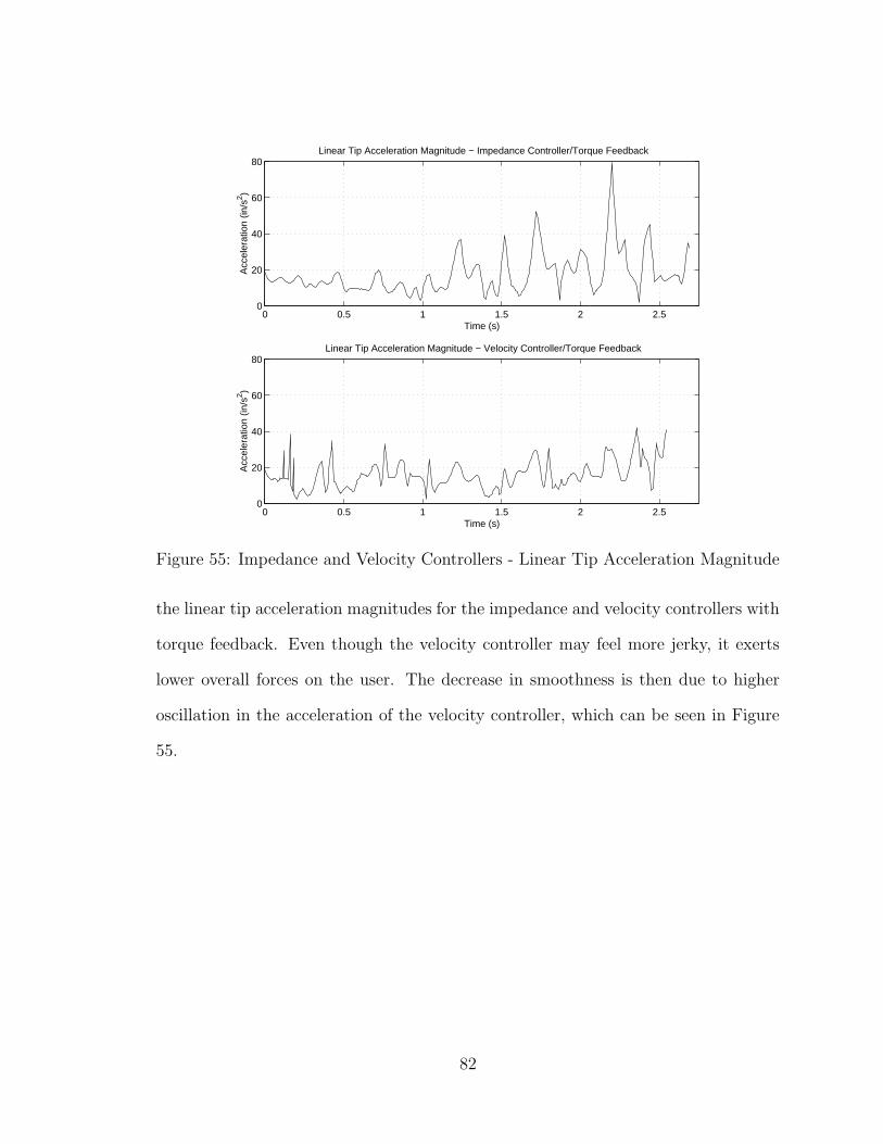
0 0.5 1 1.5 2 2.50

20

40

60

80Linear Tip Acceleration Magnitude − Velocity Controller/Torque Feedback

Time (s)

Acc

eler

atio

n (in

/s2 )

0 0.5 1 1.5 2 2.50

20

40

60

80

Time (s)

Acc

eler

atio

n (in

/s2 )

Linear Tip Acceleration Magnitude − Impedance Controller/Torque Feedback

Figure 55: Impedance and Velocity Controllers - Linear Tip Acceleration Magnitude

the linear tip acceleration magnitudes for the impedance and velocity controllers with

torque feedback. Even though the velocity controller may feel more jerky, it exerts

lower overall forces on the user. The decrease in smoothness is then due to higher

oscillation in the acceleration of the velocity controller, which can be seen in Figure

55.

82

Chapter 6

Conclusion and Future Work

6.1 Conclusion

6.2 Findings and Contributions

This work has led to two primary contributions. The first contribution is an enhanced

dynamic simulation of a controlled friction device that is modular in nature. The

second is insight into possible control concepts that could improve the performance

of PTER.

6.2.1 Dynamic Simulation

The dynamic simulation, SimPTER, has been enhanced and conceptually represents

the behavior of PTER more accurately. It may now serve as a more accurate testbed

to examine the effects of system modifications. One proposed change to PTER is to

utilize a different type of friction clutch as an actuator. By modifying the actuator

model the simulation can be used to examine the effects of such a modification on

system performance.

SimPTER’s stick-slip friction actuator modeling makes it applicable to the dy-

namic simulation of an arbitrary device where friction within an actuator serves as

the source of control forces. Its modular nature allows it to be modified and imple-

mented with respect to other systems. All that is required to do so are changes of

83

the equations of motion and the actuator model. In fact, this simulation has already

been modified to aid in the design and evaluation of a computer mouse with passive

force-feedback capability. [15]

6.2.2 Passive Interface Controllers

6.2.2.1 Proportional Torque Feedback Control

The simulated results for this controller showed a significant improvement in both

position tracking ability and smoothness. The experimental implementation on a

single clutch showed that it is possible to reduce torque following error by using

proportional feedback, but only to a certain extent. High gains caused oscillation in

the system. Simulations indicate that this limitation may be eased by using a faster

sampling rate.

Due to this oscillation at high gain, if the controller is implemented on PTER it

may not be feasible to set the gains as high as the optimal value found through simu-

lation. However, simulations showed that lower-than-optimal gains do yield increased

performance. Ultimately, if proportional torque feedback control were implemented

on PTER, performance gains are likely, though not to the full extent indicated by

the simulation.

Of course, in order for this controller to be realized, a clutch with integrated torque

measurement must be used. PTER’s current clutches do not have this capability.

6.2.2.2 Velocity Controller

Simulations using this controller along with proportional torque feedback showed

increased position tracking performance over the existing impedance controller and

lower overall levels of tip acceleration. The levels of jerk increased, however, resulting

in lower smoothness. One possible modification to the controller is to modify the

84

behavior when a clutch transitions to or from zero command input. It was shown

that higher jerk levels occur at these transitions. If the controller gradually applied

or released a clutch instead of commanding a step when turning a clutch on or off, a

more gradual change in applied torque would result, and there should be an associated

decrease in jerk. This would likely deteriorate the position tracking performance to

some extent.

6.3 Future Work

This work leaves open several related opportunities for future work, related to both

the simulation and PTER itself.

6.3.1 Simulation

The above-mentioned changes to the velocity controller could be implemented in the

simulation to determine whether or not better jerk values may be achieved, and the

associated change in position tracking performance.

Several changes to the structure of the simulation may make it a more useful tool.

First of all, currently the simulated controller is provided with the exact states of

the system. If measurement disturbances were modeled and the controller was fed a

noisy signal of the system state, the controller would more nearly mirror reality. The

performance of the controller given different levels of noise could be evaluated.

Also, the simulation could be modified to make it even more modular. Presently,

several system parameters are “hard-wired” into the simulation, such as the number of

generalized coordinates and the number of actuators. If the simulation was modified

such that every system parameter could be easily changed, it would be a more useful

and user-friendly stand-alone tool for the evaluation of controlled-friction devices.

85

6.3.2 PTER— Hardware and Software

Several modifications to the physical testbed may improve performance based on the

findings of this work. A new clutch with torque feedback could be used. This would

allow the proposed torque feedback controller to be implemented on the testbed. The

proposed velocity controller may also be implemented. Implementing either of these

controllers and gathering experimental data on their performance would allow a more

quantitative examination of the accuracy of the simulation. To do this, however, the

definition of a standard force input which could be both implemented on PTER and

modeled in the simulation is needed.

It has been shown in simulation that the static/dynamic state transitions caused

by stick-slip friction decrease the smoothness of device operation. A different com-

bination of clutch materials could be examined to minimize this effect. Delrin on

steel has been proposed as a possible candidate. According to the literature, this

combination exhibits more even friction behavior during stick-slip transitions. It is

hypothesized that such behavior would decrease the difference between dynamic and

breakaway levels of friction, and would improve the smoothness of the device.

Some non-clutch related hardware changes may also improve the performance of

the device. As shown in Chapter 4, the power supply dynamics have an influence on

the response time of the clutches. A more powerful power supply capable of delivering

higher instantaneous voltages may improve the clutch response. Such a supply would

be more able to more precisely deliver a step input current. Also, the present power

supplies have two modes of operation— a fast mode and a slow mode. Currently

the power supplies are in the slow mode. Switching them to the fast mode may

improve the transient response of the clutches. The fast mode sacrifices steady-state

performance for a quicker response time. Since PTER typically does not maintain

86

any clutches at steady-state values (other than zero), such a sacrifice may increase

overall performance.

In addition to the power supply, PTER’s sensors could be reevaluated. Currently

the only existing sensors that measure the state of the system are a potentiometer

on each of the two main links. Velocity and acceleration information are obtained

by differentiation of the position signal, which introduces noise. The potentiometers

could be replaced by rotary encoders to obtain a cleaner and more precise measure

of link position. If a very clean velocity signal is desired, for the velocity controller

for example, tachometers could be utilized on the main links.

87

Appendix A

Friction Model Calculation of Clutch

Torques

This Appendix contains the equations used to compute the static required clutch

torques for Cases 1-6 as listed in Table 7. They are all derived by solving the equations

of motion of the system under constraints on link angular acceleration. Static torques

for Case 7 cannot be solved with this method since it yields an indeterminate system.

Cases 2, 3, and 4 were broken into subcases in order to group similar conditions

together. Case 2 represents situations where a single direct clutch (coupling a link

to ground) is in the stick mode and all others are in the slip mode. In Case 3, a

single coupled clutch (coupling links A and B together) is sticking and all others

are slipping. Case 4 deals with conditions where a single direct clutch and a single

coupled clutch are stuck.

A.1 Case 1

Static calculations are not needed for this case, as none of the clutches are in the stick

mode.

88

Case # Clutch 1 Mode Clutch 2 Mode Clutch 3 Mode Clutch 4 Mode1 slip/NA slip/NA slip/NA slip/NA2.1 stick slip/NA slip/NA slip/NA2.2 slip/NA stick slip/NA slip/NA3.1 slip/NA slip/NA stick slip/NA3.2 slip/NA slip/NA slip/NA stick4.1 stick NA stick NA4.2 stick NA NA stick4.3 NA stick stick NA4.4 NA stick NA stick5 stick stick NA NA6 NA NA stick stick7 stick stick stick stick

Table 7: The 12 Possible Modes of PTER (N/A = not applied)

A.2 Case 2.1

Clutch one is in the stick mode, all others are in the slip mode. The condition for

clutch one to remain stuck is

θ1 = 0 (54)

Solving the resulting equations of motion yields

τ1required =(

M12

M22

)

τ2 −(

M12

M22

+ 1)

τ3 +(

M12

M22

− 1)

τ4 (55)

+(

M12

M22

)

τinB − τinA + V1 (56)

A.3 Case 2.2

Clutch two is in the stick mode, all others are in the slip mode. The condition for

clutch two to remain stuck is

θ2 = 0 (57)


τ2required =(

M21

M11

)

τ1 −(

M21

M11

+ 1)

τ3 +(

M21

M11

− 1)

τ4 (58)

89

+(

M21

M11

)

τinA − τinB + V2 (59)

A.4 Case 3.1

Clutch three is in the stick mode, all others are in the slip mode. The condition for

clutch three to remain stuck is

θ1 = θ2 (60)

solving the resulting equations of motion yields

τ3required =(

1

M11 + M12 + M21 + M22

)

· (61)

(M21 + M22) (−τ1 − τinA + V1) +

(M11 + M12) (τ2 + τinB − V2) + (M11 + M12 − M21 − M22) τ4

A.5 Case 3.2

Clutch three is in the stick mode, all others are in the slip mode. The condition for

clutch three to remain stuck is

θ1 = −θ2 (62)

solving the resulting equations of motion yields

τ4required =(

1

−M11 + M12 + M21 − M22

)

· (63)

(M22 − M21) (τ1 + τinA − V1) +

(M11 − M12) (τ2 + τinB − V2) + (−M11 + M12 − M21 + M22) τ3

A.6 Case 4

This case covers the condition when one direct clutch (1 or 2) and one coupling clutch

(3 or 4) are in the stick mode and all others are not applied. Since two clutches are

90

locked in this case, the following two conditions apply for all four subcases:

θ1 = 0 (64)

θ2 = 0 (65)

Following are the solved equations of motion when the listed clutches are in the stick

mode:

clutches1, 3

τ1required = τinB

τ3required = −τinA − τinB

(66)

clutches1, 4

τ4required = −τinB

τ1required = −τinA + τinB

(67)

clutches2, 3

τ3required = −τinA

τ2required = −τinA − τinB

(68)

clutches2, 4

τ4required = −τinA

τ2required = τinA − τinB

(69)

A.7 Case 5

In this case, clutches 1 and 2 are sticking and the clutches 3 and 4 are not applied.

The conditions for clutches 1 and 2 to remain stuck are

θ1 = 0 (70)

θ2 = 0 (71)


τ1required = −τinA (72)

τ2required = −τinB (73)

91

A.8 Case 6

In this case, clutches 1 and 2 are not applied and clutches 3 and 4 are sticking. The

conditions for clutches 3 and 4 to remain stuck are

θ1 = 0 (74)

θ2 = 0 (75)


τ4required =−τinA − τinB

2(76)

τ3required =−τinA + τinB

2(77)

92

Appendix B

Friction Model Validation -

Reduced-Order Tests

This Appendix contains the results of the reduced-order validation tests of the clutch

friction model.

93

B.1 Clutch 1

Constant DOFActual Path

-40 -30 -20 -10 0

0

5

10

15

20

25

30

X (in)

Y (in

)


0 1 2 30

20

40

60


Time (s)0 1 2 3

-1

-0.5

0

0.5


Time (s)

0 1 2 3-1

-0.5

0

0.5


Time (s)0 1 2 3

-1

-0.5

0

0.5


Time (s)


-40 -30 -20 -10 0

0

5

10

15

20

25

30

X (in)

Y (in

)


0 1 2 30

20

40

60


Time (s)0 1 2 3

0

5

10


Time (s)

0 1 2 3-1

-0.5

0

0.5


Time (s)0 1 2 3

-1

-0.5

0

0.5


Time (s)


94

B.2 Clutch 2

-30 -25 -20 -15 -10 -5 0

20

25

30

35

40

45

X (in)

Y (in

)


0 1 2 3-1

-0.5

0

0.5


Time (s)0 1 2 3

0

20

40

60


Time (s)

0 1 2 3-1

-0.5

0

0.5


Time (s)0 1 2 3

-1

-0.5

0

0.5


Time (s)


-30 -25 -20 -15 -10 -5 0

20

25

30

35

40

45

X (in)

Y (in

)


0 1 2 30

10

20


Time (s)0 1 2 3

0

20

40

60


Time (s)

0 1 2 3-1

-0.5

0

0.5


Time (s)0 1 2 3

-1

-0.5

0

0.5


Time (s)


95

B.3 Clutch 3

-35 -30 -25 -20

20

25

30

35

X (in)

Y (in

)


0 1 2-1

-0.5

0

0.5


Time (s)0 1 2

-1

-0.5

0

0.5


Time (s)

0 1 20

20

40

60


Time (s)0 1 2

-1

-0.5

0

0.5


Time (s)


-35 -30 -25 -20

20

22

24

26

28

30

32

34

X (in)

Y (in

)


0 1 2-1

-0.5

0

0.5


Time (s)0 1 2

-1

-0.5

0

0.5


Time (s)

0 1 20

20

40

60


Time (s)0 1 2

0

10

20


Time (s)


96

B.4 Clutch 4

-25 -20 -15 -10 -5 0 5 10 15

15

20

25

30

35

40

45

X (in)

Y (in

)


0 1 2-1

-0.5

0

0.5


Time (s)0 1 2

-1

-0.5

0

0.5


Time (s)

0 1 2-1

-0.5

0

0.5


Time (s)0 1 2

0

20

40

60


Time (s)


-25 -20 -15 -10 -5 0 5 10 15

10

15

20

25

30

35

40

45

X (in)

Y (in

)


0 1 2-1

-0.5

0

0.5


Time (s)0 1 2

-1

-0.5

0

0.5


Time (s)

0 1 20

10

20

30


Time (s)0 1 2

0

20

40

60


Time (s)


97

Bibliography

[1] B. Armstrong-Helouvry, P. DuPont, and C. Canudas de Wit. A survey of mod-

els, analysis tools, and compensation methods for the control of machines with

friction. Automatica, 30(7):1083–1138, 1994.

[2] H. Asada and J.-J. E. Slotine. Robot Analysis and Control. John Wiley and

Sons, New York, 1986.

[3] L. Cangemi, M. Cocu, and M. Raous. Adhesion and friction model for the

fiber/matrix interface of a composite. ASME Journal of Engineering Systems

Design and Analysis, 76:157–163, 1996.

[4] R. A. Charles. The development of the passive trajectory enhancing robot.

Master’s thesis, Georgia Institute of Technology, March 1994.

[5] P. R. Dahl. A solid friction model. Technical report, Aerospace Corporation, El

Segundo, CA, 1968.

[6] H. T. Davis. An investigation of passive actuation for trajectory control. Master’s

thesis, Georgia Institute of Technology, June 1996.

[7] H. T. Davis and W. J. Book. Torque control of a redundantly actuated passive

manipulator. In Proceedings of the American Control Conference, pages 959–963,

Albuquerque, NM, June 1997.

[8] M. Driels and P. Beierl. A finite memory model for haptic teleoperation. IEEE

Transactions on Systems, Man, and Cybernetics, 24(4):690–698, April 1994.

98

[9] W. K. Durfee, M. Goldfarb, A. W. Wiegner, and N. Walsh. Preliminary evalua-

tion of a controlled-brake orthosis for regulating fes-aided gait. IEEE Engineering

in Medicine and Biology, 1993.

[10] E. Bruce Goldstein. Sensation and Perception. Brooks/Cole, fifth edition, 1999.

[11] M. W. Gomes. An examination of control algorithms for a dissipative passive

haptic interface. Master’s thesis, Georgia Institute of Technology, March 1997.

[12] D. A. Haessig Jr. and B. Friedland. On the modeling and simulation of friction.

ASME Journal of Dynamic Systems, Measurement, and Control, 113:534–362,

1991.

[13] D. Karnopp. Computer simulation of stick-slip friction in mechanical dynam-

ic systems. ASME Journal of Dynamic Systems, Measurement, and Control,

107:100–103, 1985.

[14] M. A. Peshkin, J. E. Colgate, and C. Moore. Passive robots and haptic displays

based on nonholonomic elements. In Proceedings of the IEEE International Con-

ference on Robotics and Automation, pages 551–556, April 1996.

[15] E. Romagna. Design of a passive haptic mouse. Master’s thesis, Georgia Institute

of Technology, March 1999.

[16] N. Sepheri, F. Sassani, P. D. Lawrence, and A. Ghasempoor. Simulation and ex-

perimental studies of gear backlash and stick-slip friction in hydraulic excavator

swing motion. ASME Journal of Dynamic Systems, Measurement, and Control,

118:463–467, 1996.

99

[17] D. K. Swanson and E. Romagna. Development of a dynamic and control sim-

ulation of PTER, a passively actuated robot. Projet fin d’etudes (pfe), Ecole

Nationale Superieure d’Arts et Metiers, Paris, France, July 1998.

[18] J. Troccaz, S. Lavallee, and E. Hellion. A passive arm with dynamic constraints:

A solution to safety problems in medical robotics? In IEEE International Con-

ference on Systems, Man, and Cybernetics, volume 3, pages 116–171, 1993.

[19] W. R. Uttal. Teleoperators. Scientific American, pages 124–129, Dec 1989.

[20] B. G. Witmer and M. J. Singer. Measuring presence in virtual environments: A

presence questionnaire. Presence: teleoperators and virtual environments, pages

225–240, June 1998.

[21] J.-Y. Yen, C.-J. Huang, and S.-S. Lu. Stability of pfd controller with stick-slip

friction device. ASME Journal of Dynamic Systems, Measurement, and Control,

119:486–490, 1997.

100

Dynamic Simulation of an Improved Passive Haptic Display · Dynamic Simulation of an Improved...

Documents

Transcript of Dynamic Simulation of an Improved Passive Haptic Display · Dynamic Simulation of an Improved...