Dynamic Ridehailing with Electric Vehicles

Nicholas D. Kullman1, Martin Cousineau2, Justin C. Goodson3, and Jorge E. Mendoza2

1Universite de Tours, LIFAT EA 6300, CNRS, ROOT ERL CNRS 7002, Tours, France2HEC Montreal and CIRRELT, Montreal, Canada

3Richard A. Chaifetz School of Business, Saint Louis University, Saint Louis, MO

Abstract

We consider the problem of an operator controlling a fleet of electric vehicles for use in a ridehailingservice. The operator, seeking to maximize profit, must assign vehicles to requests as they arise aswell as recharge and reposition vehicles in anticipation of future requests. To solve this problem,we employ deep reinforcement learning, developing policies whose decision making uses Q-valueapproximations learned by deep neural networks. We compare these policies against a reoptimization-based policy and against dual bounds on the value of an optimal policy, including the value of anoptimal policy with perfect information which we establish using a Benders-based decomposition.We assess performance on instances derived from real data for the island of Manhattan in New YorkCity. We find that, across instances of varying size, our best policy trained with deep reinforcementlearning outperforms the reoptimization approach. We also provide evidence that this policy maybe effectively scaled and deployed on larger instances without retraining.

1 Introduction

Governmental regulations as well as a growing population of environmentally conscious consumers haveled to increased pressure for firms to act sustainably. This pressure is particularly high in the logisticsdomain, which accounts for about one third of emissions in the United States (Office of Transportationand Air Quality 2019). Ridehailing services offer a means to more sustainable transportation, promisingto reduce the need for vehicle ownership, offering higher vehicle utilization (Lyft 2018), allowing transitauthorities to streamline services (Bahrami et al. 2017), and stimulating the adoption of new vehicletechnologies (Jones and Leibowicz 2019). In recent years, ridehailing services have seen rapid andwidespread adoption, with the number of daily ridehailing trips more than quadrupling in New YorkCity from November 2015 to November 2019 (New York City Taxi & Limousine Commission 2018).

Simultaneously, electric vehicles (EVs) are beginning to replace internal-combustion engine (ICE)vehicles, commanding increasingly more market share (Edison Electric Institute 2019). Coupling thepressures to act sustainably with EVs’ promise of lower operating costs, ridehail companies are likelyto be among the largest and earliest adopters of EV technology. Indeed most major ridehail companieshave made public commitments to significant EV adoption (Slowik et al. 2019). However, EVs posetechnological challenges to which their ICE counterparts are immune, such as long recharging times andlimited recharging infrastructure (Pelletier et al. 2016).

In this work, we consider these challenges as posed to an operator of a ridehail company whose fleetconsists of EVs. We further assume that the EVs in the fleet are centrally controlled and coordinated.

1

While fleet control is somewhat centralized today, it is likely to become increasingly centralized as ridehailcompanies adopt autonomous vehicles (AVs). As with EVs, ridehail companies are likely to be amongthe earliest and largest adopters of AVs, as they stand to offer many benefits including reduced operatingcosts and greater efficiency and predictability (Fagnant and Kockelman 2015). For brevity, we refer tothis problem as the Electric Ridehail Problem with Centralized control, or E-RPC.

Our contributions in this work are as follows: 1) We offer the first application of deep reinforcementlearning (RL) to the E-RPC, developing policies that respond in real time to serve customer requests andanticipate uncertain future demand under the additional constraints of fleet electrification. The policiesare model-free, meaning they learn to anticipate this demand without any prior knowledge of its shape.We compare these deep RL-based policies to a reoptimization-based policy from the ridehailing literature.2) We evaluate these policies on instances constructed with real data reflecting ridehailing operationsfrom New York City in 2018. 3) We establish a dual bound for the dynamic policies using a perfectinformation relaxation that we solve using a Benders-like decomposition. We compare this complex dualbound against a simpler dual bound and provide an analysis of when the additional complexity of theperfect information bound is valuable. 4) We show that our best deep RL-based solution significantlyoutperforms the benchmark reoptimization policy. 5) We further demonstrate that the best-performingdeep RL-based policy can be scaled to larger problem instances without additional training. This isencouraging for operators of ridehail companies, as it suggests robustness to changes in the scale ofoperations: in the event of atypical demand or a change in the number of vehicles (e.g., due to fleetmaintenance), the policy should still provide reliable service.

We begin by reviewing related literature in §2, then provide a formal problem and model definitionin §3. We describe our solution methods in §4, the bounds established to gauge the effectiveness of thesemethods in §5, and demonstrate their application in computational experiments in §6. We offer briefconcluding remarks in §7.

2 Related Literature

Ridehail problems (RPs), those addressing the operation of a ridehailing company, fall under the broadercategory of dynamic vehicle routing problems (VRPs). Within dynamic VRPs, they may be classifiedas a special case of the dynamic VRP with pickups and deliveries or, more precisely, a special case ofthe dynamic dial-a-ride problem. Recent technological advances in mobile communications have drivennew opportunities in ridehailing and other mobility-on-demand (MoD) services, reinvigorating researchin this area. As a result, there now exists a substantial body of literature specifically pertaining to MoDapplications within the dial-a-ride domain. This literature is the focus of our review. For a broadersurvey of the dynamic dial-a-ride literature, we refer the reader to Ho et al. (2018), and, similarly, forthe dynamic VRP literature, to Psaraftis et al. (2016).

Often studies of RPs focus their investigation on the assignment problem, wherein the operator mustchoose how to assign fleet vehicles to new requests. For example, Lee et al. (2004) propose the use ofreal-time traffic data to assign the vehicle which can reach the request fastest. A study by Bischoff andMaciejewski (2016) uses a variant of this assignment heuristic that accounts for whether demand exceedssupply (or vice versa), as well as vehicles’ locations within the service region. Seow et al. (2009) proposea decentralized heuristic that gathers multiple requests and allows vehicles to negotiate with one anotherto determine which vehicles serve the new requests. They show that it outperforms heuristics like thosein Lee et al. (2004) and Bischoff and Maciejewski (2016). Hyland and Mahmassani (2018) introduce a

2

suite of optimization-based assignment strategies and show that they outperform heuristics that do notemploy optimization. Following suit, Bertsimas et al. (2019) describe ways to reduce the complexity ofoptimization-based approaches for problems with large fleets and many customers. They demonstratetheir proposed methods on realistically-sized problem instances that reflect ridehailing operations in NewYork City.

The aforementioned studies largely ignore the task of repositioning idle vehicles in anticipation offuture demand. This is in contrast to studies such as Miao et al. (2016), Zhang and Pavone (2016), andBraverman et al. (2019) who address their RP from the opposing perspective of the fleet repositioningproblem. Miao et al. (2016) do so using learned demand data with a receding horizon control approach.Braverman et al. (2019) use fluid-based optimization methods for the repositioning of idle vehicles tomaximize the expected value of requests served. They establish the optimal static policy and prove thatit serves as a dual bound for all (static or dynamic) policies under certain conditions. Other studiesconsider strategies for both the assignment and repositioning tasks. Fagnant and Kockelman (2014)propose rule-based heuristic strategies while most others (such as Alonso-Mora et al. 2017, Dandl et al.2019, and Horl et al. 2019) employ various optimization-based methods. Because it is scalable and well-suited for adaptation to our problem model, we implement the approach from Alonso-Mora et al. (2017)here as a benchmark against which to compare our proposed solution methods.

A recent competing method to address ridehail problems is reinforcement learning (RL), predomi-nantly deep reinforcement learning. As it is better-positioned to address problems with larger fleet sizes,many studies employing RL take a multi-agent RL (MARL) approach (Oda and Tachibana 2018, Odaand Joe-Wong 2018, Holler et al. 2019, Li et al. 2019, Singh et al. 2019). In work sharing many similaritiesto ours, Holler et al. (2019) use deep MARL with an attention mechanism to address both the assignmentand repositioning tasks. They compare performance under two different MARL approaches: one in whicha system-level agent coordinates vehicle actions to maximize total reward; and one in which vehicle-levelagents act individually, each maximizing its own reward. Oda and Joe-Wong (2018) use a deep MARLapproach to tackle fleet repositioning, but rely on a myopic heuristic to perform assignment. Oda andTachibana (2018) do so as well, but employ special network architectures with soft-Q learning which theyargue better accommodates the inherent complexities in road networks and traffic conditions. Li et al.(2019) employ a multi-agent RL framework, comparing two approaches that vary in what individualvehicles know regarding the remainder of the fleet; however, in contrast to most MARL applicationsto RPs, they address only the assignment problem, assuming that the vehicles are de-centralized andtherefore not repositioned by the operator. Similarly assuming de-centralized vehicles and addressingonly the assignment problem, Xu et al. (2018) combine deep RL with the optimization-based methodsused in, e.g., Alonso-Mora et al. (2017), Zhang et al. (2017), and Hyland and Mahmassani (2018). Intheir work, Xu et al. use deep RL to learn the objective coefficients in a math program that is used inan optimization framework to assign vehicles to requests.

Missing from all aforementioned studies is fleet electrification — none take into account the technicalchallenges associated with electric vehicles, such as long recharging times or limited recharging infras-tructure. The number of studies that consider these constraints is limited but growing. Most (e.g., Junget al. 2012; Chen et al. 2016; Kang et al. 2017; Iacobucci et al. 2019; La Rocca and Cordeau 2019)use the heuristic and optimization methods previously mentioned. We focus here on three works closelyrelated to ours that employ learning-based approaches. First, Al-Kanj et al. (2018) use approximatedynamic programming to learn a hierarchical interpretation of a value function that is used to determinewhether or not to recharge vehicles at their current location, in addition to repositioning decisions toneighboring grid cells and the assignment of vehicles to nearby requests. The study examines the possi-

3

bility for riders or the operator to reject a trip assignment at various costs; it also studies the problem offleet sizing. Second, Pettit et al. (2019) use deep RL to learn a policy determining when an EV shouldrecharge its battery and when it should serve a new request. The study includes time-dependent energycosts. However, it only considers a single vehicle, and it ignores the task of repositioning the vehicle inanticipation of future requests. Finally, Shi et al. (2019) apply deep reinforcement learning to the RPwith a community-owned fleet, in which they seek to minimize customer waiting times and electricityand operating costs. Similar to many of the RL studies cited previously, the study employs a multi-agentRL framework that produces actions for each vehicle individually which are then used in a centralizeddecision-making mechanism to produce a joint action for the fleet. The joint actions assign vehicles torequests and specify when vehicles should recharge; however the study also ignores repositioning actions.

Thus, ours marks the first application of deep reinforcement learning to the E-RPC in consideration ofEV constraints alongside both fleet repositioning and assignment tasks. We also argue that we consider amore realistic problem environment than in most RL-based approaches to ridehail problems. Indeed, thevast majority of studies (e.g., Al-Kanj et al. 2018; Oda and Tachibana 2018; Holler et al. 2019; Shi et al.2019; Singh et al. 2019) rely on a coarse grid-like discretization to describe the underlying service region.This serves as the basis for their repositioning actions, which are often restricted to only the adjacentgrid cells. This is in contrast to the current work, in which we allow repositioning to non-adjacent sitesthat correspond to real charging station locations. Time discretization can also be overly coarse. Manystudies choose one minute between decision epochs, as in, for example, Oda and Joe-Wong (2018); butsome choose far longer between decision epochs, such as six minutes in Shi et al. (2019) and 15 minutesin Al-Kanj et al. (2018). Given that current ridehailing applications provide fast, sub-minute responses,such an arrangement would likely lead to customer dissatisfaction. We are free of such a discretizationhere, allowing agents to respond to customer requests immediately.

3 Problem Definition and Model

We consider a central operator controlling a homogeneous fleet of electric vehicles V = {1, 2, . . . , V } thatserve trip requests arising randomly across a given geographical region and over an operating horizonT . Across the region are uncapacitated charging stations (CSs, or simply stations) C = {1, 2, . . . , C} atwhich vehicles may recharge or idle when not in service. The operator assigns vehicles to requests asthey arise. Additionally, the operator manages recharging and repositioning operations in anticipationof future requests. The objective is to maximize expected profit across the operating horizon.

Several assumptions and conditions connect the problem to real-world operations. When a newrequest arises, the operator responds immediately, either rejecting the request or assigning it to a vehicle.A vehicle is eligible to serve a new request if it can pickup within w∗ time units, the amount of timecustomers are willing to wait. Each vehicle maintains at most one pending trip request. Thus, a vehicleeither serves a newly assigned request immediately or does so after completing the service of a request towhich it is already assigned (“work-in-process”). Assignments of requests to vehicles cannot be canceled,rescheduled, or reassigned. Each vehicle has a maximum battery capacity Q and known charging rate,energy consumption rate, and speed. The operator ensures assignments and repositioning movementsare energy feasible.

We formulate the problem as a Markov decision process (MDP) whose components are defined asfollows.

4

States.

A decision epoch k ∈ {0, 1, . . . ,K} begins with a new trip request or when a vehicle finishes its work-in-process, whichever occurs first. The system state is captured by the tuple

s = (st, sr, sV). (1)

The current time st = (t, d) is the time of day in seconds t and the day of week d. If the epochwas triggered by a new request, then sr = ((ox, oy), (dx, dy)) consists of the Cartesian coordinates forthe request’s origin and destination, otherwise sr = ∅. The vector sV = (sv)v∈V describes the stateof each vehicle in the fleet. For a vehicle v, sv = (x, y, q, j(1)

m , j(1)o , j

(1)d , j

(2)m , j

(2)o , j

(2)d , j

(3)m , j

(3)o , j

(3)d ),

consisting of the Cartesian coordinates of the vehicle’s current position x, y; its charge q ∈ [0, Q]; anda description of its current activity (or job) j(1), as well as potential subsequent jobs j(2) and j(3),which may or may not exist, as determined by the operator. The description of a job j(i) consists ofits type j(i)

m ∈ {idle, charge, reposition, preprocess, serve, ∅} (equivalently, {0, 1, 2, 3, 4, ∅}; “preprocess”refers to when a vehicle is en route to pickup a customer), as well as the coordinates of the job’s originj

(i)o = (j(i)

o,x, j(i)o,y) and destination j

(i)d = (j(i)

d,x, j(i)d,y). We limit the number of tracked jobs in the state to

three, because this is the maximum number of scheduled jobs a vehicle can have given the constraintthat a vehicle may have at most one pending trip request: if a vehicle is currently serving a request andhas a pending request, then it will have jobs of type j(1)

m = 4, j(2)m = 3, and j(3)

m = 4. Note that we do notallow vehicles currently preprocessing for one request to be assigned a second (this would indeed requiretracking a fourth job). With a sufficiently strict customer service requirement (i.e., the time betweenreceipt of a customer’s request and a vehicle’s arrival to the customer), the number of opportunities tomeet that requirement after undergoing the necessary (preprocessing, serving, preprocessing) sequenceis small enough as to warrant the situation’s exclusion. If a vehicle has n < 3 scheduled jobs, then weset j(i)

m = j(i)o = j

(i)d = ∅ for n < i ≤ 3. We note that a null job j

(i)m = ∅ is distinct from an idle job

j(i)m = 0. A null job is the absence of an assignment, whereas an idle job reflects an assignment to reside

at a particular location.An episode begins with the system initialized in state s0 in epoch 0 at time 0 on some day d with no

new request (sr = ∅) and all vehicles idling with some charge at a station (v ∈ C, q ∈ [0, Q], j(1)m = idle,

j(2)m = j

(3)m = ∅ for all v ∈ V). The episode terminates at some epoch K in state sK when the time

horizon T has been reached.

Actions.

When the process occupies state s, the set of actions A(s) defines feasible assignments of vehicles to a newrequest as well as potential repositioning and recharging movements. An action a = (ar, a1, . . . , av, . . . , aV )is a vector comprised of components ar ∈ V ∪{∅} denoting which vehicle serves new request sr as well asa repositioning/recharging assignment av for each vehicle v indicating the station to which it should berepositioned and begin recharging av ∈ C ∪ {∅}. ar = ∅ denotes rejection of the new request (if it exists)and av = ∅ denotes the “no operation” (NOOP) action for vehicle v, meaning it proceeds to carry outits currently assigned jobs. We refer to the vehicle-specific repositioning/recharging/NOOP actions avas RNR actions. Jobs of type idle (0), charge (1), reposition (2), and ∅ are preemptable, meaning theycan be interrupted by a new assignment from the operator, whereas jobs of type preprocess (3) and serve(4) are non-preemptable.

The following conditions characterize A(s). If there is no new request (sr = ∅), then ar = ∅. Ifthere is a new request, then a vehicle is eligible for assignment if it can be dispatched immediately

5

Table 1: Eligible actions for an EV v.Action Eligibility conditionsServe request Request exists, no pending service (j(2)

m < 3), energy feasible, time feasibleReposition to av No active or pending service (j(1)

m < 3), energy feasibleNOOP Always, unless just finished serving and no pending service (j(1)

m = ∅)

(j(1)m ∈ {0, 1, 2, ∅}) or if it is currently servicing a customer (j(1)

m = 4) and can then be dispatched(j(2)m /∈ {3, 4}). Further, a vehicle-request assignment must be energy feasible and must arrive to the

customer within w∗ time units, the maximum amount of time a customer is willing to wait. Let fq(sv, sr)be the charge with which vehicle v will reach a station after serving request sr. fq(sv, sr) is equal to thecurrent charge of vehicle v, minus the charge required for the vehicle to travel to the origin of the newrequest (minus the charge needed to first drop off its current customer, if j(1)

m = 4), to the destinationof the new request, and then to the nearest c ∈ C from the destination. Let ft(sv, sr) be the durationof time required for vehicle v to arrive at the customer. ft(sv, sr) is equal to the time for vehicle vto travel to the origin of the new request from its current location (plus the time to first drop off itscurrent customer, if j(1)

m = 4). An assignment of vehicle v to request sr is feasible if fq(sv, sr) ≥ 0 andft(sv, sr) ≤ w∗. Repositioning and recharging movements must also be energy feasible and may notpreempt existing service assignments. If a vehicle is currently serving or preparing to serve a request(j(1)m ∈ {3, 4}), or if the vehicle has been selected to serve the new request (ar = v), then we only allow

the NOOP action av = ∅. Otherwise, we allow repositioning to any station c ∈ C that can be reachedgiven the vehicle’s current charge level. Lastly, if a vehicle completes a trip request, triggering a newepoch, and that vehicle has not been assigned a subsequent trip request (j(1)

m = ∅), then it must receivea repositioning action (av 6= ∅). This condition forces vehicles to idle only at stations. While this mayseem restrictive, we note (i) that the instances in our computational experiments (§6) contain a highdensity of stations, (ii) that cities would likely prefer that idling ridehail vehicles do so only at dedicatedlocations, and (iii) that non-CS idling locations can easily be included in our model as CSs at whichenergy is replenished at a sufficiently small rate. We summarize the eligible actions for an EV in Table 1.

Reward Function.

When the process occupies state s and action a is selected, we earn the reward C(s,a). This reward isequal to the revenue generated by serving a new request (if ar 6= ∅), minus any traveling costs incurredduring the subsequent epoch. Specifically, the revenue earned by serving new request sr consists of a basefare CB and a fare proportional to the distance of the request CD · d(sr), where CD is the per-distancerevenue and d(sr) is the distance from the request’s origin to its destination. The traveling costs incurredare CT · δ(s,a), where CT is a per-distance travel cost incurred by the operator and δ(s,a) is the totaldistance traveled by the fleet in the subsequent epoch, including all repositioning and service-relatedtravel. We note that this value is stochastic, since the time of the next epoch is unknown and equalto either the time of the arrival of the next request, or the next time at which a vehicle completeswork-in-process, whichever comes first.

This yields the following reward function:

C(s,a) =

−CT · δ(s,a) ar = ∅

CB + CDd(sr)− CT · δ(s,a) otherwise,(2)

6

Transition Function.

The transition from one state to the next is a function of the selected action and the event triggering thenext epoch. The subsequent state s′ is constructed by updating the current state s to reflect changes tovehicles’ job descriptions based on selected action a. Then, at time s′t, we observe either a new requests′r or a vehicle completing its work-in-process. At that time, we update the vehicle states s′V to reflectnew positions and charges. We also update vehicles’ job descriptions: if a vehicle has completed n jobsbetween time st and s′t, we left-shift vehicles’ job descriptions by n (j(i) ← j(i+n) for 1 ≤ i ≤ 3− n) andbackfill the vacated entries with null jobs (j(i)

m = j(i)o = j

(i)d = ∅ for 3− n < i ≤ 3). See Appendix A for

a more detailed description.

Objective Function.

Define a policy π to be a sequence of decision rules (Xπ0 , X

π1 , . . . , X

πK), where Xπ

k is a function mappingstate s in epoch k to an action a in A(s). We seek to provide the fleet operator with a policy π? thatmaximizes the expected total rewards earned during the time horizon, conditional on the initial state:

τ(π?) = maxπ∈Π

E

[K∑k=0

C(sk, Xπk (sk))

∣∣∣∣∣s0

], (3)

where Π is the set of all policies. As is common in reinforcement learning, we will often refer to the useror implementer of a policy as an agent.

4 Solution Methods

We consider four policies for solving the E-RPC (to which we will often refer synonymously as “agents”).These include two policies developed using deep reinforcement learning, which we describe in §4.1, andtwo benchmark policies, which we describe in §4.2.

4.1 Deep Reinforcement Learning Policies

Our two primary policies of interest leverage deep reinforcement learning (RL). The first of these usesdeep RL to determine which vehicle to assign to new trip requests and relies on optimization-based logicfor RNR decisions. We refer to this agent as deep ART (for “Assigns Requests To vehicles”) or just Dart.Our second agent we dub deep RAFTR (“Request Assignments and FleeT Repositioning”) or Drafter.Drafter uses deep RL both to assign vehicles to requests and to reposition vehicles in the fleet.

Before describing these policies in §4.1.3 and §4.1.4, we provide an overview of the basic method ofdeep reinforcement learning in §4.1.1 and a discussion of extensions to this basic method in §4.1.2.

4.1.1 Overview.

As defined in Sutton and Barto (2018), reinforcement learning refers to the process through which anagent, sequentially interacting with some environment, learns what to do so as to maximize a numericalreward signal from the environment; that is, learns a policy satisfying equation (3). In practice, theagent often achieves this by learning the value of choosing an action a from some state s, known as thestate-action pair’s Q-value (Q(s, a)), equal to the immediate reward plus the expected sum of futurerewards earned by taking action a from state s. We can express this relationship recursively following

7

from the Bellman equation:

Q(s, a) = C(s, a) + γE[

maxa′∈A(s′)

Q(s′, a′)∣∣∣∣s, a] , (4)

where s′ is the subsequent state reached by taking action a from state s and γ ∈ [0, 1) is a discountfactor applied to the value of future rewards. With knowledge of Q-values for all state-action pairs itmay encounter, the agent’s policy is then to choose the action with the largest Q-value. However, asthe number of unique state-action pairs is too large to learn and store a value for each, a functionalapproximation of these Q-values is learned. When deep artificial neural networks are used for thisapproximation, the method is called deep reinforcement learning or, more specifically, deep Q-learning(we use the terms interchangeably here). The neural network used in this process is referred to as thedeep Q-network (DQN).

Beginning with arbitrary Q-value approximations, the agent’s DQN improves through its interactionswith the environment, remembering observed rewards and state transitions, and drawing on these mem-ories to update the set of weights that define the DQN, conventionally denoted by θ. Specifically, witheach step (completion of an epoch) in the environment, the agent stores a memory which is a tuple ofthe form (s, a, r, s′), consisting of a state s, the action a taken from s, the reward earned r = C(s, a), andthe subsequent state reached s′. Once a sufficient number of memories (defined by the hyperparameterMstart) have been accumulated, the agent begins undergoing experience replay every Mfreq steps (Lin1992). In experience replay, the agent draws a random sample (of size Mbatch) from its accumulatedmemories and uses them to update its DQN via stochastic gradient descent (SGD) on its weights θ usinga loss function based on the difference

r + γ maxa′∈A(s′)

Q(s′, a′)−Q(s, a) (5)

(or simply r−Q(s, a) if s′ is terminal), where the Q-values in equation (5) are estimated using the agent’sDQN. The specific loss function and SGD optimizer used to update the weights may vary — we providethe specific implementations chosen for this work in §B.

We utilize the learned Q-values via an ε-greedy policy, wherein the agent chooses actions randomlywith some probability ε and chooses the action with the highest predicted Q-value with probability 1− ε.The value of ε is decayed from some initially large value εi at the beginning of training to some smallfinal value εf over the course of some number εN of training steps. This encourages exploration whenQ-values are unknown and exploitation as its predictions improve.

4.1.2 Implemented extensions to deep RL.

We adopt several well established extensions that improve the standard deep RL process just described.First, we utilize a more sophisticated sampling method during experience replay known as prioritizedexperience replay (PER) (Schaul et al. 2016). In PER, memories are more likely to be sampled if they aredeemed more important, i.e., if the loss associated with a memory is not yet known (because the memoryhas not yet been sampled during replay) or if the loss is large (if the agent was more “surprised” by thememory). Second, we use the double DQN (DDQN) architecture (Hasselt et al. 2016), which employsa “target” DQN for action evaluation and a “primary” DQN for action selection. The target DQN isa clone of the primary DQN that gets updated less often (every Mupdate steps), which helps break thetendency for DQNs to overestimate Q-values. Third, we employ dueling DDQN (D3QN) architecture(Wang et al. 2016), in which the DQN produces an estimate both of the value of the state and of the

8

relative advantage of each action. By producing these values independently (which together combine toyield Q-values), dueling architecture allows the agent to forgo the learning of action-specific values instates in which its decision-making is largely irrelevant. Finally, we use n-step learning (Sutton 1988),which helps to reduce error in learned Q-values. With n-step learning, the rewards r and subsequentstates s′ stored in an agent’s memories are modified: rather than using the state encountered one stepinto the future from s (s′), the subsequent state stored in the memory is that encountered n-steps intothe future (s(n)). Similarly, the reward r is replaced by the (properly discounted) sum of the next nrewards, i.e., those accumulated between s and s(n).

The process of choosing which deep RL extensions to implement and values for associated hyper-parameters is not unlike traditional heuristic approaches in transportation optimization. While simpleheuristics may suffice in simpler problems (see, e.g., Clarke and Wright 1964), more complex problemsoften demand more complex (meta)heuristics specifically tuned for a particular application (see, e.g.,Gendreau et al. 2002). Analogously, off-the-shelf deep RL may be successful in simpler problems (e.g.,Karpathy 2016), but success in more complex problems requires enhancements (e.g., Hessel et al. 2018)and is dependent on hyperparameter values (Henderson et al. 2018). The suite of deep RL extensionsadopted here and our selection of hyperparameter values (described in §B) are guided by standard values,where available, and ultimately chosen empirically over the course of the work.

4.1.3 Dart.

Our first proposed agent, Dart uses a combination of deep Q-learning and optimization-based logic tochoose an action a = (ar, (av)v∈V) from state s = (st, sr, sV).

Assigning vehicles to requests. The action ar pairing a vehicle with the new request employs adeep Q-network. We denote by ADart = V ∪ {∅} the action space for Dart’s DQN. The DQN takes asinput the concatenation of a subset of features from the state s which we represent by xDart = xt⊕xr⊕xV(“⊕” is the concatenation operator). These components are defined as follows:

xt System time : the concatenation of the relative time elapsed t/T and a one-hot vector indicatingthe day of the week d (e.g., for zero-indexed d with d = 0 corresponding to Monday, d = 6corresponding to Sunday, and d currently equal to Thursday (d = 3), the vector (0, 0, 0, 1, 0, 0, 0)).

xr Request information : the concatenation of a binary indicator for whether there is a new request1sr 6=∅; a one-hot vector indicating the location of the request’s origin; a one-hot vector indicatingthe request’s destination; and for each vehicle v, the distance v would have to travel to reach therequest’s origin (scaled by the maximum such distance so values are in [0, 1] (ineligible vehicles aregiven value 1)).

xV Vehicle information : the concatenation of xv for all vehicles v ∈ V (xV = x1 ⊕ · · · ⊕ xV ), wherethe vehicle-specific xv is itself the concatenation of the time at which its last non-preemptable jobends (scaled by 1/T ), the charge with which it will finish its last non-preemptable job (scaled by1/Q), and a one-hot vector indicating its current location.

One-hot vectors in xDart that indicate location rely on a discretization of the fleet’s operating region,as is common in other dynamic ridehail problems in the literature (e.g., Al-Kanj et al. 2018; Holler et al.2019). We denote the set of discrete locations (taxi zones (TZs)) constituting the region by L.

xDart is passed to the agent’s DQN to produce Q-value predictions. It then uses an ε-greedy policyas described in §4.1.1 to choose an ar ∈ ADart (infeasible vehicles are ignored). A schematic of Dart’sDQN is shown at left in Figure 1.

9

DQN

��

��

�1

-values(vehicle1)�

serve ∅ �1 �2

�

innerDQN

�3

requestembedder

�2

�3

vehicleembedder

vehicleembedder

vehicleembedder

�1

�2

�3

ℎ

�2

�1

�3

⊕

⊕

⊕

attention

��

�1

⊕

��

��

�1 DQN

-values�

�

�

�2

�3

∅ �1 �2 �3

Dart Drafter

�Dart

⊕

Figure 1: Schematics of the Dart and Drafter agents in the case of three vehicles and three TZs (V =3, L = 3). Elements are concatenated at intersections marked with ⊕. The Drafter schematic shows thecase where Q-values are being predicted for vehicle 1 (in yellow). Note: in practice, a single forward passwith xDrafter can be used to generate Q-values for all vehicles. We depict the process for a single vehiclehere for the sake of clarity.

RNR Actions. For RNR actions, whenever a request has been missed (sr 6= ∅ ∧ ar = ∅), Dartrepositions a stationary vehicle to the CS nearest the origin of the missed request, choosing the vehiclethat is closest to this CS. Let c∗r be the CS nearest the origin of the request; V ⊆ V be the subset of thevehicles that are either idling or charging at a CS (j(1)

m ∈ {0, 1}); ft(sv, sr) be the time for vehicle v toreach the origin of the request; and c∗v be the CS nearest vehicle v. Then Dart’s setting of RNR actionscan be stated as

av =

c∗r sr 6= ∅ ∧ ar = ∅ ∧ v = arg min

v∈V ft(sv, sr)

∅ j(1)m 6= ∅

c∗v otherwise.

(6)

In equation (6), the first case specifies the repositioning of the nearest eligible vehicle to the CS nearestthe origin of a missed request. The second case specifies the NOOP action for all vehicles for which itis feasible (i.e., those with a valid current job), and the third case specifies that the remaining vehicles(which do not have a valid current job) are assigned to reposition to the nearest CS.

4.1.4 Drafter.

From a state s, the Drafter agent uses a DQN to choose a vehicle to serve new requests ar and to provideRNR instructions av for each vehicle v ∈ V. Whereas the number of unique actions under the control ofDart’s DQN is V + 1, for Drafter it is (V + 1)× (C+ 1)V . For non-trivial fleet sizes V , this is intractablylarge. In response, we employ a multi-agent reinforcement learning (MARL) framework which avoidsthis intractability by making separate, de-centralized Q-value predictions for each vehicle. This reducesthe number of actions under the control of Drafter’s DQN to C+ 2, corresponding to the vehicle-specificactions of relocating to each station c ∈ C, serving the request, and doing nothing. We further reducethe number of actions by using the discretization into TZs L described in §4.1.3, yielding the action

10

space ADrafter = {serve, ∅} ∪ L for Drafter’s DQN. These actions correspond respectively to serving therequest, doing nothing, and relocating to each TZ λ ∈ L. For vehicle v, we define its DQN input byxvDrafter = (xt, xr, xv, xV), where components are as defined for Dart in §4.1.3 and the redundant xv isincluded just to indicate the vehicle for which we are generating Q-values. With vehicle input xvDrafter,the DQN makes Q-value predictions Q(xvDrafter, a) for a ∈ ADrafter. These predictions are collected forall vehicles and used to make a centralized decision. A schematic of Drafter’s DQN is shown at right inFigure 1.

DQN and attention mechanism. Let us consider the prediction of Q-values for a vehicle v?. In theexample in Figure 1, v? = v1. We now also incorporate into the DQN an attention mechanism (Mnihet al. 2014) to improve the agent’s ability to distinguish the most relevant vehicles in the current state.We expand on the attention mechanism used in Holler et al. (2019) by incorporating information aboutthe current request, which is likely to influence vehicles’ relevancy. Details of our attention mechanismcan be found in the appendix, §B. The attention is used to provide an alternative representation (anembedding) of each vehicle gv ∈ Rl and the request h ∈ Rm, as well as a description of the fleet CF ∈ Rn

known as the fleet context (here l = n = 128, m = 64; see §B). These components are used to form thevector Cv? = CF ⊕ gv? ⊕ h⊕ xt which is fed to an inner DQN. This inner DQN, which has a structuresimilar to Dart’s DQN, outputs Q-values Q(xv?

Drafter, a) for a ∈ ADrafter. The process is repeated foreach v ∈ V, with each vehicle using the same attention mechanism and inner DQN (i.e., all weights areshared).

Drafter is made scalable both through its use of an MARL approach as described above, and alsoby the attention mechanism. While the MARL approach ensures that the output of the DQN doesnot depend on the size of the fleet, the attention mechanism ensures the same for the input. Morespecifically, the attention mechanism makes it possible to predict Q-values (via the inner DQN) using arepresentation of the fleet CF whose size is not determined by the number of vehicles in the fleet. Thisstructure allows Drafter to be applied to instances of a different size than those on which it was trained.For example, given a Drafter agent trained to operate a fleet of size V , if a new vehicle is purchasedand added to the fleet, or if a vehicle malfunctions and must be temporarily removed, Drafter is capableof continuing to provide service for this modified fleet of size V ′ 6= V . We assess the scalability of theDrafter agent in our computational experiments, described in §6.

Centralized decision-making. GivenQ-value predictions for all vehicles, Drafter’s centralized decision-making proceeds as follows. Let VDrafter be the set of vehicles for whom the service action has the largestQ-value. To serve the request, we choose the vehicle in VDrafter with the largest such Q-value; thisvehicle then receives NOOP for its RNR action. The remaining vehicles perform the RNR action withthe largest Q-value, with NOOP prioritized in the event of a tie (ties between repositioning actions arebroken arbitrarily). Some consideration must be given to repositioning assignments av, as the DQN pro-duces outputs in L (TZs), while actions av take values in C (stations). Given a repositioning instructionto some TZ λ? ∈ L for vehicle v, we set av to the station in λ? that is nearest to the vehicle.

Given an action a = (ar, (av)v∈V), define avDrafter to be the action in Drafter’s action space ADrafter

assigned to vehicle v:

avDrafter =

serve ar = v

L(av) otherwise,(7)

where L(av) represents the TZ that contains station av.

11

Experience Replay. As described in §4.1.2, Drafter saves state-transition memories (s,a, r, s(n)) ateach step which are later used to train its DQN via prioritized experience replay. Let xv(n)

Drafter be theDQN input for vehicle v from state s(n). Because Drafter makes V predictions at each step, our sampleof Mbatch memories leads to an effective sample size of V ∗Mbatch, where each memory (s,a, r, s(n)) =(xvDrafter, a

vDrafter, r, x

v(n)Drafter)v∈V . Note that the reward r is shared equally among all vehicles during

training, with each vehicle receiving the full amount. This was chosen to encourage cooperation amongthe fleet. Thus, for Drafter, the difference that forms the basis of its loss function (c.f. equation (5)) is

r + γ maxa′∈ADrafter

Q(xv(n)Drafter, a

′)−Q(xvDrafter, avDrafter). (8)

4.2 Benchmark Policies

We implement two policies as benchmarks against which to assess the performance of our Dart andDrafter agents. First, in §4.2.1 we describe the Random policy that chooses actions randomly, effectivelyserving as a lower bound. Then in §4.2.2 we describe the Reopt policy, a competitive benchmark fromthe ridehailing literature that leverages reoptimization to assign vehicles to requests and to repositionthe vehicles in the fleet (Alonso-Mora et al. 2017).

4.2.1 Random.

The Random policy chooses a vehicle to serve new requests (ar) uniformly from the eligible vehicles inV ∪{∅} and chooses repositioning assignments av uniformly from the eligible locations in C ∪{∅} for eachv ∈ V.

4.2.2 Reopt.

Our Reopt agent employs the reoptimization approach introduced in Alonso-Mora et al. (2017), solvingtwo mixed integer programs (MIPs) in every epoch to inform its decisions. This agent is inherentlydifferent from the other three proposed in this section. Whereas decision epochs for Dart, Drafter, andRandom are triggered by the arrival and completion of requests, the Reopt agent is afforded a decisionepoch at regular intervals (governed by the parameter Treopt; e.g., every 30 seconds). This differencerequires modifications to the problem model defined in §3.

Required model modifications. The RNR actions from which the Reopt agent may choose areidentical to those for the other agents. However, the service action ar now takes a different form. Becausethe Reopt agent pools requests for Treopt time in between decision epochs, there may now be more thanone request to which the agent must respond. Thus, ar is now a set of tuples (v, r), corresponding tomatchings between a vehicle v ∈ V ∪∅ with a request r ∈ sR, where sR is the set of requests that arrivedin the last Treopt time. A rejected request is denoted by the matching (∅, r). Each request r ∈ sR hasorigin and destination attributes as described in §3, however, we now also include the time at which itwas received tr.

Assigning vehicles to requests. To determine how to assign vehicles to requests, Reopt solves aMIP minimizing the total customer waiting time. Let ωv,r be the waiting time of customer r if vehicle vis assigned to serve it. If the current time is st, the vehicle’s state is sv, the request’s arrival time is tr,and (as in §3) the time for the vehicle to arrive to the origin of the request from its current position isft(sv, r); then we have ωv,r = (st − tr) + ft(sv, r). We define two sets of binary variables: mv,r, which

12

take value 1 if request r is served by vehicle v; and ψr, which take value 1 if request r is served by anyvehicle (is not rejected). These variables are otherwise 0. Let M be the set of (v, r) matchings that areeither energy- or time-infeasible, as defined in §3. The MIP to determine the assignment of vehicles tonew requests is then

minimize∑r∈sR

∑v∈V

ωv,rmv,r −∑r∈sR

Bψr (9)

subject to∑r∈sR

mv,r ≤ 1, ∀v ∈ V (10)∑v∈V

mv,r = ψr, ∀r ∈ sR (11)

mv,r = 0, ∀(v, r) ∈M (12)

ψr,mv,r ∈ {0, 1} (13)

The second term in the objective, equation (9), contains the large positive constant B ensuring that themodel does not unnecessarily ignore requests. Constraints (10) ensure that each vehicle is assigned to atmost one request. Constraints (11) serve both to ensure that at most one vehicle is assigned to serve eachrequest and to fix the ψr variables, denoting whether requests will be served. Constraints (12) disallowinfeasible matchings, and constraints (13) provide variable definitions.

Following the solution to this MIP, we build the set of vehicle-request matchings ar as follows. Anyrequest r for which ψr = 0 is unserved and receives the matching (∅, r). For the remaining requests (withψr = 1), we have matchings (v, r) corresponding to the non-zero mv,r variables.

RNR actions. Per the approach in Alonso-Mora et al. (2017), after assigning vehicles to requests,Reopt then solves another MIP to reposition the vehicles in the fleet. This MIP minimizes the timeto reposition idling vehicles so as to be close to the origin of any missed requests. Alonso-Mora et al.motivate this approach with the assumptions that missed requests may request again, that more requestsare likely to occur in the same area where not all requests can be satisfied, and that idling vehicles arein areas with insufficient demand. We note that our Dart agent uses a modified version of this approachfor its RNR actions as well.

Let V ⊆ V be the subset of the fleet that is either idling or charging at a station (j(1)m ∈ {0, 1}) and was

not just assigned to serve a new request in the assignment MIP (equations (9)-(13)), and let sR ⊆ sR bethe subset of the new requests which were rejected (received a matching (∅, r)). For each request r ∈ sR,define c∗r to be the station nearest its origin. Define analogous coefficients ωv,r to be the travel time forvehicle v ∈ V to reach c∗r , and let M be the analogous set of energy-infeasible repositioning assignments.We define binary variables mv,r which take value 1 if vehicle v is repositioned to station c∗r and are 0

13

otherwise. Then the MIP to determine fleet repositioning is as follows:

minimize∑r∈sR

∑v∈V

ωv,rmv,r (14)

subject to∑r∈sR

∑v∈V

mv,r = min(∣∣∣V∣∣∣ , |sR|) (15)

∑r∈sR

mv,r ≤ 1, ∀v ∈ V (16)

∑v∈V

mv,r ≤ 1, ∀r ∈ sR (17)

mv,r = 0, ∀(v, r) ∈ M (18)

mv,r ∈ {0, 1} (19)

Constraint (15) ensures that we provide the maximum number of repositioning assignments: either weprovide an assignment for all eligible vehicles, or we provide an assignment for all missed requests.Constraint set (16) ensures that each eligible vehicle is given at most one repositioning assignment, andconstraint set (17) ensures that each missed request is assigned to be the repositioning destination for atmost one vehicle. Constraints (18) disallow infeasible matchings, and constraints (19) provide variabledefinitions.

Given a solution to this MIP, Reopt makes vehicle assignments av = c∗r for any non-zero variableassignments mv,r. Any vehicle without such an assignment simply receives the NOOP action av = ∅unless not allowed, in which case the vehicle is instructed to reposition to its nearest station. Formally,

av =

c∗r mv,r = 1

∅ j(1)m 6= ∅

c∗v otherwise,

(20)

where c∗v is the closest station to vehicle v.We offer Reopt agent as a benchmark for a good, scalable dynamic policy. In general, reoptimization

approaches offer several potential advantages, foremost among them the ability to consolidate multiplecustomer requests into a single decision-making epoch. This effectively increases the amount of informa-tion with which the fleet operator can make decisions. As such, a good policy that pools requests shouldbe at least as good as a policy that serves requests immediately.

5 Dual Bounds

Assessing policy quality is hampered by the lack of a strong bound on the value of an optimal policy, adual bound. Without an absolute performance benchmark it is difficult to know if a policy’s performanceis “good enough” for practice or if additional research is required. Here, we offer two dual bounds. Firstis a bound on the value of a policy that serves all requests (§5.1), and the second is the value of anoptimal policy with perfect information, i.e., the performance achieved via a clairvoyant decision maker(§5.2).

5.1 Serve-All Bound.

We first consider the Serve-all (SA) dual bound, which is a bound on the value of a policy that servesall requests. To establish this bound, we assume that the policy is able to serve all requests without

14

incurring any setup travel costs. That is, we can simply sum the value of all observed requests, minusthe travel costs incurred to serve them: CB + (CD −CT ) · d(sr), where, as in §3, CB is the base revenueearned when serving a request, CD is the per-distance revenue earned when serving a request, CT is theper-distance travel costs incurred, and d(sr) is the distance traveled serving the request sr. We knowthat, given a fleet of sufficient size (and assuming CD ≥ CT and CB ≥ 0), an optimal policy would chooseto serve all requests, because policies seek to maximize the sum of rewards, which here are non-negativeand incurred only by serving requests. The gap between the SA dual bound and the best policy is areflection of vehicles’ extraneous traveling and the adequacy of fleet size relative to demand and canserve as justification for a ridehailing company to invest (or not) in additional vehicles.

5.2 Perfect Information Bound.

In practice, setup and some additional travel costs are unavoidable, and it is likely that not all requestscan be feasibly served. As a result, the SA bound is expected to be loose. In an attempt to establish atighter dual bound, we consider the value of an optimal policy under a perfect information (PI) relaxation.Under the PI relaxation, the agent is clairvoyant, aware of all uncertainty a priori. In the E-RPC, tohave access to PI is to know in advance all details regarding requests: their origins, destinations, andwhen they will arise. Denote such a set of known requests by R ∈ P, where P is the set of all requestsets.

In the absence of uncertainty, we can rewrite the objective function as

maxπ∈Π

E

[K∑k=0

C(sk, Xπk (sk))

∣∣∣∣∣s0

]= E

[maxπ∈Π

K∑k=0

C(sk, Xπk (sk))

∣∣∣∣∣s0

]. (21)

Notice that the perfect information problem (right-hand side of equation (21)) can be solved with the aidof simulation. We may rely on the law of large numbers — drawing random realizations of uncertainty(request sets R ∈ P), solving the inner maximization for each, and computing a sample average —to achieve an unbiased and consistent estimate of the true objective value. This value is the perfectinformation bound. It remains to solve the inner maximization.

In the absence of uncertainty that results from having access to PI, the inner maximization can besolved deterministically: with all information known upfront, no information is revealed to an agentduring the execution of a policy. As a result, there is no advantage in making decisions dynamically(step by step) rather than statically (making all decisions at time 0). This permits the use of an exactsolution via math programming, which we pursue using a Benders-based branch-and-cut algorithm inwhich at each integer node of the branch-and-bound tree of the master problem, the solution is sent tothe subproblem for the generation of Benders cuts. Here, the master problem is responsible for assigningvehicles to requests in a time-feasible manner, and the subproblem is responsible for ensuring the energyfeasibility of these assignments. Additionally, the master problem produces an estimate of the total costsincurred through a particular assignment, and the subproblem refines this cost estimate. The use ofthe Benders-based decomposition enables the solution of larger PI problems than would otherwise befeasible. We discuss the master problem in more detail in §5.2.1, the subproblem and the generation ofcuts in §5.2.2, and comment on the bound’s tractability in §5.2.3.

5.2.1 Master problem.

The master problem, responsible for time-feasible assignments of customer requests to vehicles andproviding an estimate of the total profit earned, is the MIP defined by equations (22)-(28). In it, requests

15

are represented as nodes in a directed graph G. Request nodes i and j are connected by a directed arc(i, j) when a vehicle can feasibly serve request j after request i (ignoring energy requirements). Thegraph G also contains a dummy node for each vehicle, representing the location from which it initiallydeparts. These dummy nodes are connected to request nodes for which the initial assignment of vehiclesto requests is time-feasible. The problem involves choosing arcs in G, starting from vehicles’ dummynodes, that form (non-overlapping) paths for the vehicles which indicate the sequence of requests thatvehicles will serve. If a request i is a member of some vehicle’s path, it contributes ci to the objectivefunction, the revenue that its service generates. Our objective also includes the travel costs incurredalong the paths that the vehicles travel in serving their assigned requests.

In the master problem, R is the set of all requests (known a priori given PI), V is the set of vehicles,ci is the revenue earned by serving request i, hi is a binary variable taking value 1 if request i is assignedto any vehicle, yvi is a binary variable taking value 1 if job i is the first request assigned to vehicle v, xijis a binary variable taking value 1 if a vehicle is assigned serve request j immediately after request i, ziis a continuous non-negative variable equal to the time at which a vehicle arrives to pick up request i, triis the time at which request i begins requesting service, w∗ is the maximum amount of time a customermay wait between when they submit their request and when a vehicle arrives, tpi (dpi ) is the travel time(distance) between the origin and destination of request i, and tsij (dsij) is the travel time (distance)between the destination of request i and the origin of request j. For vehicles, tpv is equal to the earliesttime at which they can depart from their initial locations, and tsvi (dsvi) is equal to the travel (distance)time between their initial locations and the origin of request i. We formally define the master problemas

maximize∑i∈R

cihi − CT

∑v∈V

∑i∈R

dsviyvi +∑i∈R

∑j∈R\{i}

dsijxij +∑i∈R

dpi hi

− θm (22)

subject to∑v∈V

yvi +∑

j∈R\{i}

xji ≥ hi, ∀i ∈ R (23)

∑j∈R\{i}

xij ≤ hi, ∀i ∈ R (24)

∑j∈R

yvj ≤ 1, ∀v ∈ V (25)

zi ≥ tri + (tpv + tsvi − tri )yvi, ∀i ∈ R,∀v ∈ V (26)

zi − zj ≥ tri − trj − w∗ + (tpj + tsji − tri + trj + w∗)xji, ∀i, j ∈ R (i 6= j) (27)

hi, xij , yvi ∈ {0, 1}; tri ≤ zi ≤ tri + w∗; θm ≥ 0 (28)

The objective (22) maximizes profit: its first term captures the revenue earned, while the remainingterms account for costs. In the objective, the first two terms in parentheses capture the distance thevehicles travel in setting up for (traveling between) requests, and the third term in parentheses capturesthe distance traveled by the vehicles while serving the requests. In its last term, the objective also includesthe continuous variable θm. This variable is controlled by optimality cuts generated in the subproblem,effectively serving to correct the master problem’s underestimation of travel costs. While the masterproblem’s objective accounts for the minimum incurred travel costs (those incurred by traveling requestsequences directly), there will likely be additional costs incurred as vehicles travel to and from stations.These station visits are required both for vehicles to restore their charge and to idle between requests,since they are not allowed to do so at request locations. Thus, intuitively, θm represents the costs incurredduring these required station detours.

16

While θm is ultimately controlled by the subproblem, we can facilitate the solution of the PI problemby improving the master problem’s estimation of these costs. To do so, we consider the minimum requireddetours between pairs of requests. For requests i and j, let k be the station requiring the minimum detourbetween i’s destination and j’s origin, and let tdij (ddij) be the time (distance) required to travel fromthe destination of request i to station k to the origin of request j. Then we define the minimum detourdistances between requests

`ij =

ddij tri + w∗ + tpi + tdij ≤ trj0 otherwise,

(29)

and then apply the following condition on θm:

θm ≥∑i∈R

∑j∈R\{i}

CT `ijxij . (30)

In equation (29) we specify that if there is sufficient time for a vehicle to perform a detour betweenrequests i and j then it must do so, and in equation (30) we account for these additional travel costs byraising the lower bound on θm.

For the remainder of the master problem, equation (23) manages the binary assignment variable hi,requiring that it be included in some vehicle’s path to take value 1. Similarly, equation (24) manages thevariables for the outgoing arcs from request i, forcing them to take value 0 if the request has not beenassigned to a vehicle. Equation (25) ensures that each vehicle has at most one request assigned to be itsfirst. Equation (26) sets a lower bound for the time at which vehicles can arrive to their initial requests,and equation (27) sets a lower bound for the time at which vehicles’ can arrive to subsequent requests.Finally, equation (28) defines variables scopes’ and bounds the earliest and latest possible start times forrequests zi.

As mentioned, we only connect request nodes i and j via directed arc (i, j) if it is time-feasible to serverequest j after request i; that is, if tri + tpi + tsij ≤ trj + w. While energy-feasibility is ultimately ensuredby the subproblem, we can again facilitate in the master problem by eliminating additional arcs in Gusing known energy consumptions to perform stronger feasibility checks. Let ρ be the maximum rate atwhich vehicles acquire energy when recharging, qpi be the energy required to travel from the origin to thedestination of request i, qsij be the energy required to travel from the destination of request i to the originof request j, qdi be the energy required to travel from the destination of request i to the nearest chargingstation, and qoi be the energy required to travel to the origin of request i from its nearest charging station.Then for arc (i, j) to exist, we require that trj +w− (tri + tpi + tsij) ≥ 1

ρ max{0, (qpj + qdj − (Q− qoi − qpi ))},

which states that the maximum down time between i and j (left-hand side) be sufficient to accommodateany recharging that must occur between these requests (right-hand side). We provide similar feasibilitychecks for the arcs (v, i) connecting vehicle dummy nodes to requests. Specifically, the simpler time-feasible check requires that vehicle v can arrive to request i in time: tpv + tsvi ≤ tri +w∗. In considerationof energy requirements, we ensure tri + w∗ − (tpv + tsvi) ≥ 1

ρ max{0, qsvi + qpi + qdi − qpv}, which states thatthe time for the vehicle to perform any required charging (right-hand side) cannot be greater than theavailable time before it must arrive to request i. Finally, we force the underlying graph to be acyclic,meaning we prohibit pairs of requests i, j such that (tri + tpi + tsij < trj + w∗) ∧ (trj + tpj + tsji < tri + w∗).

5.2.2 Subproblem.

A solution to the master problem is a sequence of request assignments rv = (r1v, r

2v, . . .) for each vehicle

v ∈ V. r1v is taken to be the element in the singleton {j| yvj = 1} ∪ ∅; subsequent entries riv are similarly

17

elements in singletons {j|xri−1v j = 1} ∪ ∅ (rv terminates with the first null element). Given sequences

for each vehicle, the subproblem must ensure they are energy feasible. To do so, we use a modifiedversion of frvcpy (Kullman et al. 2020), which implements the labeling algorithm developed by Frogeret al. (2019) to solve the Fixed Route Vehicle Charging Problem (FRVCP) (Montoya et al. 2017). TheFRVCP entails providing charging instructions (where to charge and to what amount) for an electricvehicle traversing a fixed sequence of customers. The algorithm takes as input a sequence like rv and, ifsuccessful, terminates with the minimum duration path through the sequence that includes instructionsspecifying at which charging stations to recharge and to what amount. When unsuccessful, the labelingalgorithm returns the first unreachable node in the sequence. In the original implementation customersdid not have time constraints as they do here, where vehicles are required to arrive to requests in thewindow [tri , tri + w∗]. We further discuss the algorithm and our modifications to it to accommodate thisdifference in the appendix, §C.

Unsuccessful termination of the algorithm for a sequence rv indicates that the sequence cannot betraversed energy-feasibly. To remove it from the search space, we add the following feasibility cut to themaster problem:

yv,r1v

+j?−1∑i=1

xri−1v ,ri

v< j?, (31)

where j? ≤ |rv| is the index of the first unreachable request node in rv to which the algorithm wasunable to feasibly extend a label. This cut (31) enforces that not all variables defining the subsequence(r1v, . . . , r

j?

v ) be selected.When the algorithm terminates successfully, we add optimality cuts that correct the master problem’s

estimation of the costs incurred in serving the sequence rv. Specifically, let C(rv) represent the masterproblem’s estimation of the costs incurred by traveling sequence rv,

C(rv) = CT

dsv,r1v

+|rv|−1∑i=1

dsri

v,ri+1v

+|rv|∑i=1

dpi

, (32)

and let C∗(rv) represent the actual total cost of traveling sequence rv, as determined by the solutionof the labeling algorithm. Then we add optimality cuts to the master problem that account for thedifference:

θm ≥ (C∗(rv)− C(rv))

yv,r1v

+|rv|−1∑i=1

xri−1v ,ri

v

(|rv| − 1)

. (33)

These cuts work by ensuring that if the master problem selects sequence rv, then it must account for itstrue travel costs by setting θm ≥ C∗(rv) − C(rv). Otherwise, the right-hand side of equation (33) is atmost 0, which is redundant given the non-negativity constraint on θm, equation (28).

5.2.3 Tractability of the PI Bound.

The PI bound is often computationally intractable to obtain. This is because the estimation of theexpected value with perfect information entails repeated solutions to the inner maximization of equa-tion (21), a challenging problem despite the absence of uncertainty. Even if the Benders-based methodof §5.2.1 and 5.2.2 does not return an optimal solution for a given realization of uncertainty, we may stillget a valid bound by using the best (upper) bound produced by the solver (Gurobi v8.1.1). The solver’sbound serves as a bound on the value of an optimal policy with PI, and therefore also as a bound on an

18

0000 0400 0800 1200 1600 20000K

10K

20K

30K

Figure 2: Mean number of requests by hour in Manhattan on a business day in 2018. The dashed verticalline indicates episodes’ 03:00 start time.

optimal policy. This mixed bound, effectively combining both the solver’s relaxation and an informationrelaxation, is weaker than a bound based on the information relaxation alone. However, we show incomputational experiments that it still provides value.

6 Computational Experiments

To test the solution methods proposed in §4, we perform computational experiments modeled afterbusiness-day ridehailing operations on the island of Manhattan in New York City. We describe theexperimental setup in §6.1, present our results in §6.2, and offer a brief discussion of the results in §6.3.

6.1 Experimental Setup

We generate problem instances (equivalently, episodes over which the agents act) using data publiclyavailable for the island of Manhattan in New York City. New York City Taxi & Limousine Commission(2018) provide a dataset consisting of all ridehail, Yellow Taxi, and Green Taxi trips taken in 2018.We filter the data to only those trips that originate and terminate in Manhattan and those that occuron business days (d ∈ {0, 1, 2, 3, 4} = {Mon, Tues, Weds, Thurs, Fri}, excluding public holidays). Theaverage daily profile for these data is shown in Figure 2. Based on this profile, we set the episode lengthT to 24 hours, with episodes beginning and ending at 3:00 am, as this time corresponds to a naturallull in demand from the previous day and gives agents time to perform proactive recharging before themorning demand begins. Data for each trip includes the request’s pickup time as well as the location of itsorigin and destination. Requests’ origins and destinations are given by their corresponding taxi zones, anofficial division of New York City provided by the city government (NYC OpenData 2019) that roughlydivides the city into neighborhoods. We use this as the basis for our geographical discretization L asdescribed in §4, resulting in |L| = 61 TZs for Manhattan (see Figure 3). Coordinates ((ox, oy), (dx, dy))for requests’ exact origins and destinations are drawn randomly from inside their corresponding TZs.

We fix the set of stations C to all CSs currently available or under construction in Manhattan at thetime of writing, as listed by National Renewable Energy Laboratory (2019), yielding a set of |C| = 302CSs (blue marks in left map of Figure 3). We assume that all CSs dispense energy at a constant rate of72kW, equal to that of a Tesla urban supercharger (Tesla 2017). Vehicles’ batteries have similar traitsto that of a mid-range Tesla Model 3, with a capacity of 62 kWh and an energy consumption of 0.15kWh/km. Further, we assume vehicles travel at a speed of approximately 13 km/hr (8 mi/hr), incur

19

5%

4%

3%

2%

1%

Requestdestinationdistribution

(2:00-3:00am)

Figure 3: (Left) The island of Manhattan divided into taxi zones with charging station locations shown inblue. (Right) Distribution of requests’ desintations by taxi zone during episodes’ last hour (02:00-03:00).

travel costs of $0.53/km (Bosch et al. 2018), and, when serving a request, receive a fixed reward ofCB = $10.75 and distance-dependent reward of CD = $4.02/km, under the assumption of Euclideandistances. We set the maximum time that customers are willing to wait for a vehicle to be w∗ = 5minutes. These instance parameters are summarized in Table 2.

Vehicles’ initial locations are determined by drawing a TZ randomly according to the distribution ofdrop-off locations during the final hour of the previous day’s operation (2:00-3:00am). See right mapin Figure 3. We then choose a charging station uniformly from within the TZ (TZs without CSs areexcluded). Vehicles’ initial charges are drawn uniformly from [0, Q]. To randomly generate a set of Rrequests for an instance, we first sample a business day from 2018 then draw R requests that occurredon that day.

We consider a primary set of problem instances with R = 1400 requests and V = 14 vehicles (we willoften refer to these instances by their R/V ratio, 1400/14). The number of requests was chosen suchthat the mean number of requests per hour during the busiest time of day (between 6:00-7:00pm, seeFigure 2) is approximately 100. The number of vehicles in this set was then derived from a scaling ofthe ratio R?/V ?, where R? = 449, 121 is the total number of trip requests (taxi and ridehail) served onan average business day in Manhattan in 2018, and V ? = 4, 400 is an approximation of the number ofsimultaneously active Yellow Taxis in Manhattan at any given time in 2018 (see data aggregations in,e.g., Schneider 2019). Experiments on our 1400/14 instances include results for all agents as well as theSA and PI bounds. The agents are evaluated over a set of 200 episodes, while the bounds — given thehigh computational demand for the PI bound — are established using an average over 30 episodes. Priorto evaluation, the Dart and Drafter agents are first trained on a separate set of 750 episodes. We notethat the PI bound cannot be solved to optimality for these instances, so the values reported correspondto the mixed version of the bound as described in §5.2.3.

In addition to the 1400/14 instances, we also consider instances two, five, and ten times larger(2800/28, 7000/70, and 14000/140) to assess Drafter’s ability to scale and generalize. That is, we

20

Table 2: Instance parameters.Parameter ValueEpisode length T 24 hrsEpisode start time 3:00 amNumber of Taxi Zones |L| 61Number of charging stations |C| 302CS charging rate 72 kWVehicle battery capacty 62 kWhVehicle energy consumption 0.15 kWh/kmVehicle speed 13 km/hrTravel costs CT $0.53/kmBase fare CB $10.75Per-distance fare CD $4.02/kmMax customer waiting time w∗ 5 minutes

evaluate the Drafter agent directly on 200 instances of each size without any additional training onthese instances — it simply uses its DQN as trained on the 1400/14 instances. We compare the Drafteragent to the Random and Reopt agents. Dart is absent from this analysis as its scalability is inherentlyhandicapped, with its DQN’s output (ADart) dependent on the number of vehicles in the instance. Thisis in contrast to Drafter, for which the size of its DQN output (ADrafter) is indifferent to the size of thefleet. Details on the hyperparameters used in the training of the Dart and Drafter agents for all instancesize classes are provided in §B. We use a reoptimization period of Treopt = 30 seconds for the Reoptagent.

6.2 Results

We begin with a comparison of our proposed dual bounds in §6.2.1. We then describe agents’ performanceon the instance sets, first discussing the results on our primary 1400/14 instances in §6.2.2, followed byscalability tests in §6.2.3.

6.2.1 Comparison of Dual Bounds.

The first proposed dual bound, SA, is simple to compute but may be loose when not all requests can befeasibly served. In contrast, the PI bound promises to be tighter, but it is significantly more challenging tocompute. Here, we aim to quantify the improvement in the bound afforded by the additional computationfor the PI bound.

Intuitively, with a larger fleet size V , more requests can be served. At some V , a policy with PI shouldbe able to serve all requests, so the PI and SA bounds should converge. Conversely, with decreasing fleetsize, even with PI, it should become impossible to serve all requests, so the bounds will diverge. We testthis intuition in an experiment comparing the value of these two bounds as a function of fleet size. Theresults are summarized in Figure 4. We begin with instances of size 1400/14, for which (as shown in§6.2.2) the gap between the PI and SA bounds is large. We then increment the fleet size by 2 (V+ = 2),and resolve 15 episodes of the 1400/V instances. We find that the results confirm intuition – the gapbetween the bounds decreases exponentially with increasing fleet size, reaching near equivalence (2%

21

14 16 18 20 22 24 26 28 30 32 34 36 38 40

Fleet size

0%5%

10%

15%

20%

25%

30%

35%

40%

45%

50%

Gap from PI to SA Bound

Figure 4: The mean percent difference of the SA bound relative to the PI bound over 15 episodes ofan instance with 1400 requests for varying fleet sizes. Note: computed as SA−PI

PI , where SA and PI

are (upper bounds on) the profit earned by a policy that serves all requests and an optimal policy withperfect information, respectively.

gap between the bounds) at a fleet size of 38. Because the SA bound does not include the travel costsincurred outside of serving requests, the gap between the SA and PI bounds will generally be greaterthan zero. We note that the PI values here reflect the mixed PI bound discussed in §5.2.3, implying thatthe gaps may actually be larger than these results suggest.

6.2.2 Primary 1400/14 Instance Set.

The Dart and Drafter training curves, showing their increasing objective performance over the 750training episodes, are provided in Figure 5. Dashed horizontal lines in the figure indicate the meanobjective performance of Reopt and Random, and thin vertical lines indicate the points at which theDart and Drafter agents surpass the mean performance of the Reopt agent. We see that learning happensquickly for both agents, with Dart surpassing Reopt after 96 training episodes and Drafter doing so afteronly 41 episodes. Both agents’ objective performance is stable after 250 episodes. In Figure 6 we compareagents’ performance on the 30 evaluation episodes for which the PI and SA dual bounds are available.We find that the Drafter agent is the best performing with a mean daily profit of $10,898, althoughthere remains a large gap between this policy and the PI dual bound, and an even larger gap betweenthe PI and SA dual bounds (as expected from the experiments in §6.2.1). We note that the reported PIbound is a mixed bound (see §5.2.3), as we are not able to solve any of the 30 episodes to optimality.After Drafter, Dart is the second-best performing agent, earning a mean daily profit of $9,627. Dart’sperformance is not significantly different from Reopt, which has a mean profit of $9,067. On this set of30 instances, Drafter outperforms Reopt by 20.2%.

6.2.3 Scalability Tests.

After training on the 1400/14 instances, we then apply Drafter directly to instances two, five and tentimes larger. With the primary instances of size 1400/14 being the basis with an Instance Scale of 1, werefer to these larger instances as having Instance Scales of 2, 5, and 10, which respectively correspond

22

0 250 500 750

Training Episode

$1,000

$2,000

$3,000

$4,000

$5,000

$6,000

$7,000

$8,000

$9,000

$10,000

$11,000Objective (USD)

Drafter

Dart

Reopt

Random

41 96

Figure 5: Training curves for the Dart and Drafter agents, showing two-week performance averages (theaverage objective over an episode and the previous 13 episodes). Dashed horizontal lines depict meanobjective values for the Random and Reopt agents. Vertical lines indicate where Dart and Drafter surpassReopt’s mean objective achievement.

$0 $5,000 $10,000 $15,000 $20,000 $25,000 $30,000

Objective (USD)

Random

Reopt

Dart

Drafter

PI

SA

$10,898-41.8%

$18,7360.0%

$28,18450.4%

$6,815-63.6%

$9,067-51.6%

$9,627-48.6%

Figure 6: Agents’ objective performance over 30 evaluation episodes of size 1400/14 for which dualbounds are available. Parenthesized values indicate the gap to the PI bound. Black marks indicate 95%confidence intervals.

23

Instance Scale1 2 5 10

$0

$40,000

$80,000

$120,000

$160,000

$10,937$6,794 $9,250

$16,353$23,754$27,187

$46,341

$74,313$80,345

$169,391$166,540

$99,232

RandomReoptDrafter

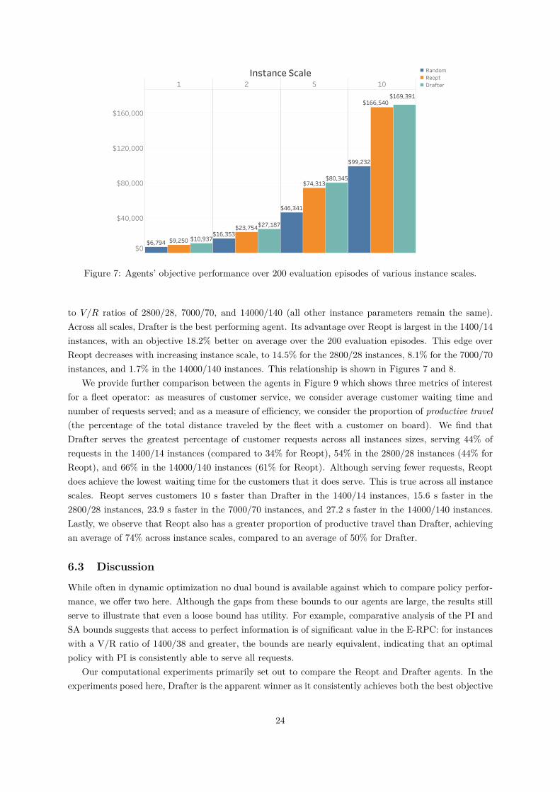
Figure 7: Agents’ objective performance over 200 evaluation episodes of various instance scales.

to V/R ratios of 2800/28, 7000/70, and 14000/140 (all other instance parameters remain the same).Across all scales, Drafter is the best performing agent. Its advantage over Reopt is largest in the 1400/14instances, with an objective 18.2% better on average over the 200 evaluation episodes. This edge overReopt decreases with increasing instance scale, to 14.5% for the 2800/28 instances, 8.1% for the 7000/70instances, and 1.7% in the 14000/140 instances. This relationship is shown in Figures 7 and 8.

We provide further comparison between the agents in Figure 9 which shows three metrics of interestfor a fleet operator: as measures of customer service, we consider average customer waiting time andnumber of requests served; and as a measure of efficiency, we consider the proportion of productive travel(the percentage of the total distance traveled by the fleet with a customer on board). We find thatDrafter serves the greatest percentage of customer requests across all instances sizes, serving 44% ofrequests in the 1400/14 instances (compared to 34% for Reopt), 54% in the 2800/28 instances (44% forReopt), and 66% in the 14000/140 instances (61% for Reopt). Although serving fewer requests, Reoptdoes achieve the lowest waiting time for the customers that it does serve. This is true across all instancescales. Reopt serves customers 10 s faster than Drafter in the 1400/14 instances, 15.6 s faster in the2800/28 instances, 23.9 s faster in the 7000/70 instances, and 27.2 s faster in the 14000/140 instances.Lastly, we observe that Reopt also has a greater proportion of productive travel than Drafter, achievingan average of 74% across instance scales, compared to an average of 50% for Drafter.

6.3 Discussion

While often in dynamic optimization no dual bound is available against which to compare policy perfor-mance, we offer two here. Although the gaps from these bounds to our agents are large, the results stillserve to illustrate that even a loose bound has utility. For example, comparative analysis of the PI andSA bounds suggests that access to perfect information is of significant value in the E-RPC: for instanceswith a V/R ratio of 1400/38 and greater, the bounds are nearly equivalent, indicating that an optimalpolicy with PI is consistently able to serve all requests.

Our computational experiments primarily set out to compare the Reopt and Drafter agents. In theexperiments posed here, Drafter is the apparent winner as it consistently achieves both the best objective

24

Instance Scale1 2 5 10

0%

10%

20%

Improvement from Reopt

18.2%

14.5%

8.1%

1.7%

Figure 8: The improvement in objective offered by Drafter over Reopt over 200 evaluation episodes ofinstances of varying scales.

Instance Scale1 2 5 10

0%

25%

50%

75%

100%

Requests Served

Instance Scale1 2 5 10

0

60

120

180

240

300

Cust Wait Time (s)

Instance Scale1 2 5 10

0%

25%

50%

75%

100%

Productive Travel

Random Reopt Dart Drafter

Figure 9: Over 200 evaluation episodes of various instance scales, agents’ performance as measured by(Left) the percent of requests that were served, (Center) the average customer waiting time, and (Right)the proportion of travel that is productive. Note that because it does not scale directly, Dart appearsonly for Instance Scale 1.

25

values and the greatest percent of customer requests served. These are arguably the most importantcriteria to an operator of a ridehail fleet. That Drafter consistently serves more requests, when takenalongside its higher waiting times (207 s on average, compared to 187 s for Reopt), suggests that Drafter isable to position the fleet so as to better cover the demand. Notably, Drafter requires no prior knowledge orassumptions about the shape of this demand to learn to do so — in the language of reinforcement learning,it is model-free. Rather than relying on, e.g., historical data or domain knowledge regarding parametersdescribing the demand’s spatial and temporal distributions, Drafter garners sufficient working knowledgeof the demand during its training to determine which actions best allow it to serve future requests andultimately achieve greater objective values. Being model-free also implies that Drafter is flexible tovarious relationships between actions and rewards, because this relationship is learned by the agent.That is, while we trained and evaluated Drafter on the reward function defined by equation (2), we couldhave equally used, e.g., a deterministic reward function or one which incorporated additional revenue orcost metrics. Although displaying inferior performance than Drafter and lacking its scalability, Dart isalso model-free and therefore enjoys these same benefits. Drafter’s scalability should be encouraging foroperators of ridehail companies, as it suggests robustness to changes in problem instances. That is, inthe event that demand is slow on a particular day or one or more vehicles are unavailable (e.g., due torepairs), Drafter should still provide reliable service.

We note the encroaching objective performance of Reopt with increasing Instance Scales relative toDrafter, with Drafter’s advantage shrinking from 18.2% in the 1400/14 instances to 1.7% in the 14000/140instances. This result is not surprising. First, Drafter is acting in an environment that is increasinglydifferent from the one in which it was trained. Additionally, with more requests pooled in a singledecision-making epoch, Reopt is armed with increasing information with which to make decisions. Thisability to wait-and-see is an innate advantage possessed by reoptimization-style agents. Future researchshould investigate these two points in more detail. For example, for the former, while we lacked thecomputational resources to do so here, it would be interesting to compare the performance of a scaledDrafter agent (like the one used here) against a Drafter agent that was trained directly on instances ofthe larger size. This would answer the question as to how much of Drafter’s relative decline was due tothe difference in its evaluation and training environments, rather than Reopt simply performing betterat scale. In the event that, under this comparison, the gap between Drafter and Reopt continues to besmaller for larger instances, then it would suggest that Reopt-style agents may simply have an advantageat larger instance scales, due to their ability to more completely observe demand before making decisions.Regardless, it would be a worthy endeavor to create an MDP problem model that would accommodatea deep-RL agent that could similarly pool requests for some amount of time before making a decision.

Lastly, we comment on the proportion of productive travel. This metric is primarily of interest tocities, as they aim to reduce congestion on roadways. Our results suggest that fleet operation costsalone may not be ample motivation for ridehail operators to minimize nonproductive travel: in thepresence of realistic revenues and prices, Drafter found that it was still in its financial interest to pursuenonproductive vehicle movements (in order to serve future requests). To combat such behavior, citiesmay wish to implement congestion pricing (see, e.g., the review in Gu et al. 2018). Future research mayinvestigate how learned agent behavior varies under different pricing schemes, as one would expect thatnonproductive travel would decrease with increased congestion pricing.

26

7 Concluding Remarks

We considered the E-RPC, the problem faced by an operator of a ridehail service with a fleet composed ofcentrally-controlled electric vehicles. To solve the E-RPC, we developed two policies, Dart and Drafter,derived with deep reinforcement learning. To serve as a comparison, we consider a reoptimization policyfrom the ridehailing literature, as well as a randomly-acting policy that serves as a lower bound. Wedevelop two dual bounds on the value of an optimal policy, including the value of an optimal policywith perfect information. To establish this bound, we decompose a relaxed version of the E-RPC intotime- and energy-feasibility subproblems, and solve them via a Benders-like decomposition. We offeran analysis of when this more complex dual bound offers value beyond that of a simpler proposed dualbound.

We perform computational experiments on instances derived from real world data for ridehail op-erations in New York City in 2018. Across instances of varying scales, we consistently find the deepRL-based Drafter agent to be the best performing. On instance scales for which it was specificallytrained, it achieved an objective 18.2% better than the reoptimization policy. We further show thatDrafter is scalable, finding that, on instances two, five, and ten times larger than any on which it wastrained, it outperforms other policies by 14.5%, 8.1%, and 1.7%, respectively. These results ultimatelysuggest there are opportunities for deep reinforcement learning in solving problems like the E-RPC. Bymore efficiently utilizing finite resources, these methods have the potential to promote greater sustain-ability in the domain of transportation and logistics.

Acknowledgements

Nicholas Kullman is grateful for support from the Societe des Professeurs Francais et Francophonesd’Amerique. Justin Goodson wishes to express appreciation for the support from the Center for SupplyChain Excellence at the Richard A. Chaifetz School of Business. Martin Cousineau and Jorge Mendozawould like to thank HEC Montreal and the Institute for Data Valorization (IVADO) for funding thatcontributed to this project; Jorge Mendoza is additionally grateful for funding from HEC Montreal’sProfessorship on Clean Transportation Analytics. This research was also partly funded by the FrenchAgence Nationale de la Recherche through project e-VRO (ANR-15-CE22-0005-01).

27

A Updating Vehicles’ Job Descriptions

Upon choosing action a from state s, we immediately update vehicles’ job descriptions. We describe thisprocess here. For the following discussion, let the current location of vehicle v be (vx, vy).

NOOP.

Vehicles receiving the NOOP instruction (av = ∅) see no change to their existing job descriptions.

Repositioning/Recharging.

Let the location to which the vehicle is instructed to reposition be av = c with location (cx, cy). We setthe first job’s type to repositioning (j(1)

m = 2), its origin to the vehicle’s current location (j(1)o = (vx, vy)),

and its destination to c (j(1)d = (cx, cy)). We then set the second job type to charging (j(2)

m = 0) whichbegins and ends at c (j(2)

o = j(2)d = (cx, cy)). After recharging, the vehicle then idles at the station:

j(3)m = 0 and j

(3)o = j

(3)d = (cx, cy).

Serving Request.

Let the new request have origin (ox, oy) and destination (dx, dy).

No work-in-process. If the vehicle is not already serving a request (j(1)m 6= 4), then its first job is

updated to type preprocess (j(1)m = 3) with origin j

(1)o = (vx, vy) and destination j

(1)d = (ox, oy). Its

second job is then serving the customer, so we set the type to serve (j(2)m = 4), the origin j(2)

o = (ox, oy),and the destination j(2)

d = (dx, dy). The vehicle’s third job is then empty, so we set j(3)m = j

(3)o = j

(3)d = ∅.

Work-in-process. If the vehicle is currently serving an existing customer (j(1)m = 4), then the first job

is unchanged. The second job is preprocess (j(2)m = 3), as the vehicle moves from the drop-off location

of its current customer (j(2)o = j

(1)d ) to the pick-up location of the new customer (j(2)

d = (ox, oy)). Thevehicle’s third job is then to serve the customer request, so we set the type to serve (j(3)

m = 4), the originj

(3)o = (ox, oy), and the destination j

(2)d = (dx, dy).

B Agent Details: Hyperparameters & Attention Mechanism

We provide here additional details about the training and implementation of the Dart and Drafteragents. Hyperparameters, chosen based on empirical results, are given in Table 3. The rest of thissection describes the attention mechanism used in Drafter’s DQN.

The attention mechanism used by the Drafter agent is depicted in Figure 1. We begin by creating anembedding gv of each vehicle’s representation xv using a single dense layer called the “vehicle embedder.”An embedding of some input is simply an alternative representation of that input. For example, fora vehicle representation xv ∈ [0, 1]2 × {0, 1}|L| (see §4.1.3) the embedder maps it to gv ∈ R128 viaf(Waxv + b), where Wa is a 128 × (2 + |L|) matrix of trainable weights, b is a 128-length vector oftrainable weights, and f is the activation function (here a rectified linear unit, ReLU ). Similar to vehicleembeddings gv, we create an embedding h ∈ R64 of the request xr using another single dense layer (the“request embedder”). We then concatenate each vehicle’s embedding gv with the request embedding h

28

Table 3: Agents’ hyperparameters.

Parameter Dart DrafterOptimizer (learning rate) Adam (0.001) Adam (0.001)Loss function Huber HuberDiscount factor γ 0.999 0.999Memory capacity 1,000,000 1,000,000Steps prior to learning Mstart 2,000 2,000Training frequency Mfreq 100 100Batch size Mbatch 32 32Initial epsilon εi 1 1Final epsilon εf 0.01 0.1Epsilon decay steps εN 75,000 75,000PER type None (uniform) proportionalPER α - 0.6PER β0 - 0.4PER beta decay steps - 600,000Target network update frequency Mupdate 5,000 5,000n-step learning 3 3DQN activation functions ReLU ReLU*Number of hidden layers (pre-dueling, advantage stack, value stack) (1,2,2) (2,2,2)**

* With the exception of the layers in the attention mechanism as described in §B.

** For the inner DQN (see Figure 1).

29

to produce joint embeddings jv = gv ⊕ h. The jvs and gvs are then used to perform attention over thevehicles, creating a fleet context vector CF ∈ R128 via

CF =∑v∈V

αvgv, (34)

where αv = σ(w · tanh(W · jv)) is a scalar weighting vehicle v, σ is the sigmoid activation function, w isa trainable vector of weights, and W is a trainable matrix of weights (the summation in equation (34)is performed element-wise). This attention mechanism is similar to the one used to produce the fleetcontext in Holler et al. (2019), with the notable difference that here we also incorporate the request.As the request sr is likely to influence which vehicles are relevant in a given state, its inclusion in theattention mechanism should yield a more descriptive fleet context CF . The fleet context vector is thenused in the production of Q-values for each vehicle as described in §4.1.4.

C Froger et al. (2019) FRVCP Labeling Algorithm

We provide here additional details on the labeling algorithm from Froger et al. (2019) and our modifi-cations to accommodate time constraints on the customers. We will refer to the sequence of requests tobe served by vehicle v, as determined by the master problem (§5.2), by rv = (r1

v, r2v, . . .).

C.1 Algorithm Overview

To find the optimal recharging instructions given a request sequence rv, the FRVCP is reformulatedas a resource-constrained shortest path problem. The algorithm then works by setting labels at nodeson a graph G′v (see example in Figure 10) that reflects the vehicle’s assigned request sequence rv andpossible charging station visits. Labels are defined by state-of-charge (SoC) functions. SoC functions arepiecewise-linear functions comprised of supporting points z = (zt, zq) that describe a state of departurefrom a node in G′v in terms of time zt and battery level zq. See Figure 11 for an example.

During the algorithm’s execution, labels are extended along nodes in G′v. When extending labels, SoCfunctions are shifted by the travel time and energy between nodes, and supporting points resulting ininfeasible (negative) charges are pruned. When extending a label to a charging station node, we createnew supporting points that correspond to the breakpoints in the charging curve at that station – energylevels at which the charging rate changes. (Note that here, we assume linear charging until the vehiclereaches full battery, at which point it begins idling. This breakpoint corresponds to z2 in the left graphof Figure 11.) We continue to extend labels along nodes in G′v until either the destination node r|rv|

v isreached or there are no feasible label extensions. If the destination node is reached, the algorithm returnsthe earliest arrival time to that node based on the label’s SoC function and the sequence is deemed to beenergy feasible; if the destination node cannot be reached, the sequence is deemed energy-infeasible andthe algorithm returns the first request node to which it could not extend a label. Bounds on energy andtime are established in pre-processing and are used alongside dominance rules during the algorithm’sexecution in order to improve its efficiency. For complete details on the algorithm, we refer the readerto Froger et al. (2019).

C.2 Algorithm Modifications

We modify the algorithm to accommodate time constraints for the requests in rv, which are not consideredin the original implementation. We assume that the vehicle is eligible to depart its initial location, denoted

30

Sequencenodes Chargingstations

0��1�

B

A

�2�

B

A

�3�

B

A′

�

Figure 10: A depiction of the graph G′v for a vehicle assigned to serve three customer requests. In theexample, we assume there are two stations, A and B, at which the vehicle can recharge.

0v, at time tpv with charge qpv . Moving between locations a and b requires energy qsa,b and time tsa,b (ifb is a request, the values reflect the time and energy to reach its destination via its origin). For thisdiscussion, additional information about the algorithm beyond the overview in §C.1 may be necessary,for which we refer the reader to the description of Algorithm 3 in §5.3 and Appendix E of Froger et al.(2019).

The first modification serves to include the option of idling at charging stations. We add a point inthe charging function at (∞, Q) as shown in Figure 11. This allows the vehicle to idle at a CS after ithas fully charged its battery. Second, when extending a label to a request, we prune supporting pointsat the request node based on the request’s time constraints. Specifically, all supporting points that aretoo early are shifted later in time. This may result in multiple supporting points with the same timebut different energy levels, in which case we keep only the supporting point with maximum energy.Supporting points whose times are too late are eliminated, and a new supporting point is establishedwhere the SoC function intersects the end of the customer’s time window. These processes are shownin Figure 11. Finally, when extending a label from one request node directly to another, if a supportingpoint has been shifted later in time by some amount ∆t (like z′′1 in Figure 11), then the point incursa charge penalty ∆q. This reflects the constraint that vehicles may not idle at request nodes, so weassume that the vehicle has continued driving (e.g., “circling the block”) during the time ∆t and hasthus drained its battery by the amount ∆q. Note that such penalties are not incurred when extendingto or from charging station nodes in G′v as these nodes have no time constraints.

31

= ( + (� − ),�)�2 ��1

1

��

�

1

= (∞, )�3 ��

2

= ( , − )�1 ��,�0�

��� ��

,�0�SoCatdeparture

Timeatdeparture

�′

2�′

3

�′

1

( , − )��

�,�1�

��

�,�1� �″

2

�

�″

1

Figure 11: SoC functions for labels extended from 0v to B to r1v. (Left) The SoC function at B

after arriving directly from 0v with supporting points corresponding to immediate departure withoutrecharging (z1), recharging completely (z2), and subsequent indefinite idling (z3). (Center) These pointsare then shifted by (tsB,r1

v,−qsB,r1

v) as we extend a label to r1

v, resulting in points z′1, z′2, z′3. (Right)Supporting points must lie within customer r1

v’s time window w∗. Point z′1 is eliminated since it isdominated after this shift (indicated by the “x”), having less charge than the new point z′′1 . Point z′3 iseliminated and the new point z′′2 is created where the SoC function intersects the end of the time window.Note that there is no charge penalty incurred here, as the label is being extended from a charging station.

32

ReferencesLina Al-Kanj, Juliana Nascimento, and Warren B Powell. Approximate dynamic programming for planning a

ride-sharing system using autonomous fleets of electric vehicles. arXiv preprint arXiv:1810.08124, 2018.

Javier Alonso-Mora, Samitha Samaranayake, Alex Wallar, Emilio Frazzoli, and Daniela Rus. On-demand high-capacity ride-sharing via dynamic trip-vehicle assignment. Proceedings of the National Academy of Sciences,114(3):462–467, 2017.

Omid Bahrami, Jim Gawron, Jack Kramer, and Bob Kraynak. Flexbus: Improving public transitwith ride-hailing technology, December 2017. http://sustainability.umich.edu/media/files/dow/

Dow-Masters-Report-FlexBus.pdf, Accessed December 2019.

Dimitris Bertsimas, Patrick Jaillet, and Sebastien Martin. Online vehicle routing: The edge of optimization inlarge-scale applications. Operations Research, 67(1):143–162, 2019.

Joschka Bischoff and Michal Maciejewski. Simulation of city-wide replacement of private cars with autonomoustaxis in berlin. Procedia Computer Science, 83:237–244, 2016.

Patrick M Bosch, Felix Becker, Henrik Becker, and Kay W Axhausen. Cost-based analysis of autonomous mobilityservices. Transport Policy, 64:76–91, 2018.

Anton Braverman, Jim G Dai, Xin Liu, and Lei Ying. Empty-car routing in ridesharing systems. OperationsResearch, 67(5):1437–1452, 2019.

T Donna Chen, Kara M Kockelman, and Josiah P Hanna. Operations of a shared, autonomous, electric vehiclefleet: Implications of vehicle & charging infrastructure decisions. Transportation Research Part A: Policyand Practice, 94:243–254, 2016.

Geoff Clarke and John W Wright. Scheduling of vehicles from a central depot to a number of delivery points.Operations research, 12(4):568–581, 1964.

Florian Dandl, Michael Hyland, Klaus Bogenberger, and Hani S Mahmassani. Evaluating the impact of spatio-temporal demand forecast aggregation on the operational performance of shared autonomous mobilityfleets. Transportation, 46(6):1975–1996, 2019.

Edison Electric Institute. Electric vehicle sales: Facts and figures, October 2019. https://www.eei.org/

issuesandpolicy/electrictransportation/Documents/FINAL_EV_Sales_Update_Oct2019.pdf, AccessedJanuary 2020.

Daniel J Fagnant and Kara Kockelman. Preparing a nation for autonomous vehicles: opportunities, barriers andpolicy recommendations. Transportation Research Part A: Policy and Practice, 77:167–181, 2015.

Daniel J Fagnant and Kara M Kockelman. The travel and environmental implications of shared autonomousvehicles, using agent-based model scenarios. Transportation Research Part C: Emerging Technologies, 40:1–13, 2014.

Aurelien Froger, Jorge E Mendoza, Ola Jabali, and Gilbert Laporte. Improved formulations and algorithmiccomponents for the electric vehicle routing problem with nonlinear charging functions. Computers &Operations Research, 104:256–294, 2019.

Michel Gendreau, Gilbert Laporte, and Jean-Yves Potvin. Metaheuristics for the capacitated VRP. In PaoloToth and Daniele Vigo, editors, The vehicle routing problem, chapter 6, pages 129–154. SIAM, 2002.

Ziyuan Gu, Zhiyuan Liu, Qixiu Cheng, and Meead Saberi. Congestion pricing practices and public acceptance:A review of evidence. Case Studies on Transport Policy, 6(1):94–101, 2018.

H.V. Hasselt, A. Guez, and D. Silver. Deep reinforcement learning with double q-learning. In Proceedings of the30th AAAI Conference on Artificial Intelligence, pages 2094–2100. AAAI Press, 2016.

Peter Henderson, Riashat Islam, Philip Bachman, Joelle Pineau, Doina Precup, and David Meger. Deep rein-forcement learning that matters. In 32nd AAAI Conference on Artificial Intelligence, pages 3207–3214.AAAI Press, 2018.

33

Matteo Hessel, Joseph Modayil, Hado Van Hasselt, Tom Schaul, Georg Ostrovski, Will Dabney, Dan Horgan,Bilal Piot, Mohammad Azar, and David Silver. Rainbow: Combining improvements in deep reinforcementlearning. In 32nd AAAI Conference on Artificial Intelligence, pages 3215–3222. AAAI Press, 2018.

Sin C Ho, WY Szeto, Yong-Hong Kuo, Janny MY Leung, Matthew Petering, and Terence WH Tou. A surveyof dial-a-ride problems: Literature review and recent developments. Transportation Research Part B:Methodological, 111:395–421, 2018.

John Holler, Risto Vuorio, Zhiwei Qin, Xiaocheng Tang, Yan Jiao, Tiancheng Jin, Satinder Singh, Chenxi Wang,and Jieping Ye. Deep reinforcement learning for multi-driver vehicle dispatching and repositioning problem.arXiv preprint arXiv:1911.11260, 2019.

Sebastian Horl, Claudio Ruch, Felix Becker, Emilio Frazzoli, and Kay W Axhausen. Fleet operational policiesfor automated mobility: A simulation assessment for zurich. Transportation Research Part C: EmergingTechnologies, 102:20–31, 2019.

Michael Hyland and Hani S Mahmassani. Dynamic autonomous vehicle fleet operations: Optimization-basedstrategies to assign avs to immediate traveler demand requests. Transportation Research Part C: EmergingTechnologies, 92:278–297, 2018.

Riccardo Iacobucci, Benjamin McLellan, and Tetsuo Tezuka. Optimization of shared autonomous electric ve-hicles operations with charge scheduling and vehicle-to-grid. Transportation Research Part C: EmergingTechnologies, 100:34–52, 2019.

Erick C Jones and Benjamin D Leibowicz. Contributions of shared autonomous vehicles to climate changemitigation. Transportation Research Part D: Transport and Environment, 72:279–298, 2019.

Jaeyoung Jung, R Jayakrishnan, and Keechoo Choi. Shared-taxi operations with electric vehicles. Institute ofTransportation Studies Working Paper Series, Irvine, Calif, 2012.

Namwoo Kang, Fred M Feinberg, and Panos Y Papalambros. Autonomous electric vehicle sharing system design.Journal of Mechanical Design, 139(1):011402, 2017.

Andrej Karpathy. Deep reinforcement learning: Pong from pixels, May 2016. http://karpathy.github.io/

2016/05/31/rl/, Accessed January 2020.

Nicholas Kullman, Aurelien Froger, Jorge E. Mendoza, and Justin C. Goodson. frvcpy: An open-source solverfor the fixed route vehicle charging problem. INFORMS Journal on Computing, 2020. In press.

Charly Robinson La Rocca and Jean-Francois Cordeau. Heuristics for electric taxi fleet management at teo taxi.INFOR: Information Systems and Operational Research, 0(0):1–25, 2019.

Der-Horng Lee, Hao Wang, Ruey Long Cheu, and Siew Hoon Teo. Taxi dispatch system based on currentdemands and real-time traffic conditions. Transportation Research Record, 1882(1):193–200, 2004.

Minne Li, Zhiwei Qin, Yan Jiao, Yaodong Yang, Jun Wang, Chenxi Wang, Guobin Wu, and Jieping Ye. Efficientridesharing order dispatching with mean field multi-agent reinforcement learning. In The World Wide WebConference, pages 983–994. ACM, 2019.

Long-Ji Lin. Self-improving reactive agents based on reinforcement learning, planning and teaching. Machinelearning, 8(3-4):293–321, 1992.

Lyft. Why 130,000 lyft passengers were ready to ditch their personal cars in less than 24 hours, December 2018.https://blog.lyft.com/posts/ditchyourcardata, Accessed December 2019.

Fei Miao, Shuo Han, Shan Lin, John A Stankovic, Desheng Zhang, Sirajum Munir, Hua Huang, Tian He, andGeorge J Pappas. Taxi dispatch with real-time sensing data in metropolitan areas: A receding horizoncontrol approach. IEEE Transactions on Automation Science and Engineering, 13(2):463–478, 2016.

Volodymyr Mnih, Nicolas Heess, Alex Graves, and Koray Kavukcuoglu. Recurrent models of visual attention.In Proceedings of the 27th International Conference on Neural Information Processing Systems-Volume 2,pages 2204–2212. MIT Press, 2014.

34

Alejandro Montoya, Christelle Gueret, Jorge E Mendoza, and Juan G Villegas. The electric vehicle routingproblem with nonlinear charging function. Transportation Research Part B: Methodological, 103:87–110,2017.

National Renewable Energy Laboratory. Alternative fuels data center, 2019. Data retrieved 09/2019from https://www.nyserda.ny.gov/All-Programs/Programs/Drive-Clean-Rebate/Charging-Options/

Electric-Vehicle-Station-Locator.

New York City Taxi & Limousine Commission. TLC trip record data, 2018. Data retrieved 09/2019 fromhttps://www1.nyc.gov/site/tlc/about/tlc-trip-record-data.page.

NYC OpenData. NYC taxi zones, 2019. Data retrieved 09/2019 from https://data.cityofnewyork.us/

Transportation/NYC-Taxi-Zones/d3c5-ddgc.

Takuma Oda and Carlee Joe-Wong. Movi: A model-free approach to dynamic fleet management. In IEEEINFOCOM 2018-IEEE Conference on Computer Communications, pages 2708–2716. IEEE, 2018.

Takuma Oda and Yulia Tachibana. Distributed fleet control with maximum entropy deep reinforcement learning.In NeurIPS 2018 Machine Learning for Intelligent Transportation Systems Workshop, 2018.

Office of Transportation and Air Quality. U.S. Transportation Sector Greenhouse Gas Emissions 1990-2017, June2019. URL https://nepis.epa.gov/Exe/ZyPDF.cgi?Dockey=P100WUHR.pdf. EPA-420-F-19-047.

Samuel Pelletier, Ola Jabali, and Gilbert Laporte. 50th anniversary invited article – goods distribution withelectric vehicles: Review and research perspectives. Transportation Science, 50(1):3–22, 2016.

Jacob F Pettit, Ruben Glatt, Jonathan R Donadee, and Brenden K Petersen. Increasing performance of electricvehicles in ride-hailing services using deep reinforcement learning. arXiv preprint arXiv:1912.03408, 2019.

Harilaos N Psaraftis, Min Wen, and Christos A Kontovas. Dynamic vehicle routing problems: Three decades andcounting. Networks, 67(1):3–31, 2016.

T. Schaul, J. Quan, I. Antonoglou, and D. Silver. Prioritized experience replay. In 4th International Conferenceon Learning Representations, 2016.

Todd W. Schneider. Taxi and ridehailing usage in new york city, 2019. https://toddwschneider.com/

dashboards/nyc-taxi-ridehailing-uber-lyft-data/, Accessed September 2019.

Kiam Tian Seow, Nam Hai Dang, and Der-Horng Lee. A collaborative multiagent taxi-dispatch system. IEEETransactions on Automation Science and Engineering, 7(3):607–616, 2009.

Jie Shi, Yuanqi Gao, Wei Wang, Nanpeng Yu, and Petros A Ioannou. Operating electric vehicle fleet for ride-hailing services with reinforcement learning. IEEE Transactions on Intelligent Transportation Systems,2019.

Ashutosh Singh, Abubakr Alabbasi, and Vaneet Aggarwal. A distributed model-free algorithm for multi-hop ride-sharing using deep reinforcement learning. In NeurIPS 2019 Machine Learning for Autonomous DrivingWorkshop, 2019.

Peter Slowik, Lina Fedirko, and Nic Lutsey. Assessing ride-hailing company commitments to electrifi-cation, February 2019. https://theicct.org/sites/default/files/publications/EV_Ridehailing_

Commitment_20190220.pdf, Accessed January 2020.

Richard S Sutton. Learning to predict by the methods of temporal differences. Machine learning, 3(1):9–44,1988.

R.S. Sutton and A.G. Barto. Reinforcement Learning: An Introduction. Adaptive Computation and MachineLearning series. MIT Press, 2018. ISBN 9780262352703.

Tesla. Supercharging cities, 2017. https://www.tesla.com/blog/supercharging-cities, Accessed December2019.

Z. Wang, T. Schaul, M. Hessel, H.V. Hasselt, M. Lanctot, and N.D. Freitas. Dueling network architectures fordeep reinforcement learning. In Maria Florina Balcan and Kilian Q. Weinberger, editors, Proceedings of

35

The 33rd International Conference on Machine Learning, volume 48, pages 1995–2003, New York, NewYork, USA, 20–22 Jun 2016. PMLR.

Zhe Xu, Zhixin Li, Qingwen Guan, Dingshui Zhang, Qiang Li, Junxiao Nan, Chunyang Liu, Wei Bian, and JiepingYe. Large-scale order dispatch in on-demand ride-hailing platforms: A learning and planning approach. InProceedings of the 24th ACM SIGKDD International Conference on Knowledge Discovery & Data Mining,pages 905–913. ACM, 2018.

Lingyu Zhang, Tao Hu, Yue Min, Guobin Wu, Junying Zhang, Pengcheng Feng, Pinghua Gong, and Jieping Ye. Ataxi order dispatch model based on combinatorial optimization. In Proceedings of the 23rd ACM SIGKDDInternational Conference on Knowledge Discovery and Data Mining, pages 2151–2159. ACM, 2017.

Rick Zhang and Marco Pavone. Control of robotic mobility-on-demand systems: A queueing-theoretical perspec-tive. The International Journal of Robotics Research, 35(1-3):186–203, 2016.

36