Dynamic Programming, Tree-width and Computation onGraphical Models

byBrian Oliveira Lucena

M.S., Brown University 1998A.B., Harvard University 1996

ThesisSubmitted in partial fulÞllment of the requirements for

the Degree of Doctor of Philosophyin the Division of Applied Mathematics at Brown University

May 2002

c! Copyrightby

Brian Oliveira Lucena2002

Abstract of �Dynamic Programming, Tree-width and Computation on Graphical Models,�by Brian Oliveira Lucena, Ph.D., Brown University, May 2002

Computing on graphical models is a Þeld of diverse interest today, due to the generalapplicability of these models. This thesis begins by giving background on the generalizedDynamic Programming (DP) method of performing inference computations (Chapter 1).We then (in Chapter 2) demonstrate explicity equivalences between different methods ofcomputation and the importance of a parameter called tree-width. We go on to prove anovel method of bounding the tree-width of a graph by using maximum cardinality search.This gives a lower bound on the computational complexity of a graph with respect to stan-dard methods. This bound can be quite weak or quite good. We provide experimentalresults demostrating both cases. Chapter 3 is concerned with Coarse-to-Fine DynamicProgramming (CFDP), a method which can be faster than the standard methods, butrequires special conditions. We prove theorems giving the complexity of CFDP for prob-lems that meet certain criteria. These theoretical results are borne out with applicationsto speciÞc problems.

This dissertation by Brian Oliveira Lucena is accepted in its present form bythe Division of Applied Mathematics as satisfying the

dissertation requirement for the degree ofDoctor of Philosophy

DateStuart Geman, Director

Recommended to the Graduate Council

DateDavid Mumford, Reader

DateBasilis Gidas, Reader

Approved by the Graduate Council

DatePeder J. Estrup

Dean of the Graduate School and Research

iii

The Vita of Brian Oliveira Lucena

Brian Oliveira Lucena was born on January 17, 1975 in Suffern, NY. He attended SpringValley High School in Spring Valley, NY, and graduated as valedictorian in June 1992.He then entered Harvard University, graduating in 1996 magna cum laude in AppliedMathematics / Probability and Statistics. After spending another year in Cambridge,MA doing research and teaching, he entered the Applied Mathematics program at BrownUniversity in September, 1997. He received the Masters degree in Applied Mathematicsin May, 1998 and defended this Ph.D. thesis on April 26, 2002.

iv

Acknowledgments

It is an impossible endeavor to thank every person who played a role in my Ph.D.thesis and the long process leading up to its defense, but nonetheless an attempt must bemade.

My advisor, Stuart Geman gave me a fantastic combination of guidance and indepen-dence from start to Þnish. His enthusiasm kept me excited throughout the process and hetruly served as a role model for me as a scientist, teacher and person.

Various other professors, notably Basilis Gidas, David Mumford and Elie Bienenstockwere available for conversations and discussion on a variety of topics, both mathemati-cal and non-mathematical. Laura Leddy, Jean Radican, Roselyn Winterbottom, TrudeeTrudell, and the rest of the administrative staff were unfailingly helpful in numerous ca-pacities.

My three roommates at 18 University Avenue each warrant particular mention. Aso-han Amarasingham has been a constant presence for me in the 5 years I�ve spent inProvidence, at various times as classmate, roommate, officemate, and above all, as afriend. The seemingly inÞnite number of conversations on countless subjects we�ve hadin various locations in the Western Hemisphere have been some of the greatest times I�vehad. Kamran Diba brought the four of us together at 18 University and exposed us to avariety of music, wine, and life theories while making our house a community instead ofjust a residence. The intensity of his irresolute convictions and his questioning of everyfacet of life forced me to open my mind to new ideas. Carlos Vicente with his irrepressibleenergy supplied endless amounts of amusement and entertainment. His kind critiques ofmy fashion sense made me a better dresser (for a while) and his lust for life never failedto cheer me up.

A couple of fellow students are owed special debts for their direct contributions to thisthesis. Matthew Harrison made the original conjecture of the main theorem in Chapter 2,which sent me down a path of discovery which has not quite ended. He also served as mypersonal reference for questions on MATLAB and Latex. Luis Ortiz provided invaluablereferences, thoroughly proofread the tree-width results, and helped me see things from�the computer science point of view�. Eyal Amir, a postdoc at UC-Berkeley, supplied mewith the CYC, HPKB, and CPCS graphs.

I should also thank the countless good friends I�ve made here, including Phil Weickert,Govind Menon, Joel Middleton, Mickey Inzlicht, Naomi Ball, Rusty Tchernis, Julie Esdale,Stephanie Munson, Andrew Huebner, Danny Trelogan, Sameer Parekh, Nick Costanzinoand so many others I can�t possibly list them all. You have all made living these 5 yearsin Providence not only tolerable, but indeed, the happiest in my life to date.

Most importantly, I thank my family. My brother John and sister Anyssa included mein their travels and events, and provided their own �Þnancial aid� to do things I otherwisecouldn�t afford to do on a graduate student stipend. My parents always encouraged meto go my own way and Þnd my own path. The debt I owe to you can never be repaid.

v

Contents

Acknowledgments v

1 Introduction and Tutorial 11.1 Introduction . . . . . . . . . . . . . . . . . . . . . . . . . . . . . . . . . . . . 21.2 Generalized Dynamic Programming Tutorial . . . . . . . . . . . . . . . . . . 5

1.2.1 Computing the Most Likely ConÞguration . . . . . . . . . . . . . . . 61.2.2 Computing all Marginal Distributions . . . . . . . . . . . . . . . . . 10

2 Tree-width and Computational Complexity 152.1 Introduction . . . . . . . . . . . . . . . . . . . . . . . . . . . . . . . . . . . . 162.2 Generalized DP, Junction trees, and complexity . . . . . . . . . . . . . . . . 16

2.2.1 Equivalence Results . . . . . . . . . . . . . . . . . . . . . . . . . . . 182.2.2 Tree width . . . . . . . . . . . . . . . . . . . . . . . . . . . . . . . . 21

2.3 Computing and bounding tree-width . . . . . . . . . . . . . . . . . . . . . . 252.3.1 Maximum Cardinality Search . . . . . . . . . . . . . . . . . . . . . . 252.3.2 Main Result . . . . . . . . . . . . . . . . . . . . . . . . . . . . . . . . 26

2.4 The MCS lower bound . . . . . . . . . . . . . . . . . . . . . . . . . . . . . . 312.4.1 Properties of the MCS Lower Bound . . . . . . . . . . . . . . . . . . 32

2.5 Improving the Bound . . . . . . . . . . . . . . . . . . . . . . . . . . . . . . . 322.5.1 Edge Contraction . . . . . . . . . . . . . . . . . . . . . . . . . . . . . 332.5.2 Empirical results . . . . . . . . . . . . . . . . . . . . . . . . . . . . . 352.5.3 Low Density Parity Check code graphs . . . . . . . . . . . . . . . . . 36

2.6 Conclusions . . . . . . . . . . . . . . . . . . . . . . . . . . . . . . . . . . . . 39

3 Complexity Results and Applications for Coarse-to-Fine Dynamic Pro-gramming 403.1 Introduction . . . . . . . . . . . . . . . . . . . . . . . . . . . . . . . . . . . . 413.2 Explanation of the method . . . . . . . . . . . . . . . . . . . . . . . . . . . 413.3 Continuous Framework . . . . . . . . . . . . . . . . . . . . . . . . . . . . . . 46

3.3.1 DeÞnitions and Notation . . . . . . . . . . . . . . . . . . . . . . . . . 473.3.2 Main results (chain graph) . . . . . . . . . . . . . . . . . . . . . . . 51

3.4 Example � the isoperimetric problem . . . . . . . . . . . . . . . . . . . . . . 533.4.1 Empirical results . . . . . . . . . . . . . . . . . . . . . . . . . . . . . 56

3.5 General Graph Structures . . . . . . . . . . . . . . . . . . . . . . . . . . . . 583.6 Multi-dimensional example . . . . . . . . . . . . . . . . . . . . . . . . . . . 60

3.6.1 Results . . . . . . . . . . . . . . . . . . . . . . . . . . . . . . . . . . 63

vi

List of Figures

1.1 A graph G. . . . . . . . . . . . . . . . . . . . . . . . . . . . . . . . . . . . . 6

2.1 Tπ(G) for π = (a, b, c, d, f, e, g, h). The solid edges were in EG and thedotted edges are in Fπ(G). . . . . . . . . . . . . . . . . . . . . . . . . . . . 19

2.2 Lines demonstrate edges that must exist in H . . . . . . . . . . . . . . . . . 282.3 Lines demonstrate edges that must exist in H . . . . . . . . . . . . . . . . . 292.4 A graph . . . . . . . . . . . . . . . . . . . . . . . . . . . . . . . . . . . . . . 312.5 An example of edge contraction. . . . . . . . . . . . . . . . . . . . . . . . . 332.6 Edge contraction of the corners of a lattice . . . . . . . . . . . . . . . . . . 332.7 Examples of square and triangular lattices for n=4 . . . . . . . . . . . . . . 362.8 An MRF for a LDPC code with n=10, m=5, k=3 . . . . . . . . . . . . . . . 37

3.1 A MRF with respect to a chain graph and the associated trellis. . . . . . . 423.2 Four trellises in various stages of the CFDP process. Dotted edges represent

edges with a value of 0. . . . . . . . . . . . . . . . . . . . . . . . . . . . . . 453.3 The �legality� tree of height 4. . . . . . . . . . . . . . . . . . . . . . . . . . 503.4 The area enclosed by one segment. . . . . . . . . . . . . . . . . . . . . . . . 543.5 The initial trellis for the isoperimetric problem with n = 8 and R = 8. . . . 563.6 Our computational results for the isoperimetric problem. . . . . . . . . . . . 573.7 A spring network. Black dots are Þxed points and white dots are moveable

points. . . . . . . . . . . . . . . . . . . . . . . . . . . . . . . . . . . . . . . . 603.8 The MRF dependendy graph for the spring problem. . . . . . . . . . . . . . 613.9 The computational results for the spring problem. . . . . . . . . . . . . . . 63

vii

Chapter 1

Introduction and Tutorial

1

2

1.1 Introduction

The ultimate goal of mathematical modeling is to understand and predict the behavior ofsystems. In deterministic systems we can more or less predict exactly what will happen.In probabilistic systems, however, there is an inherent uncertainty. Thus our goal isto understand the uncertainty; that is, to learn about the distribution of the variableof interest. This distribution will change and become �less� random as we have moreinformation about the variable. Graphical models such as Markov random Þelds, Bayesnets, and a host of other variations are attempts to model complex systems of randomvariables and their interactions, with the goal of understanding and making predictions.

The Þeld of graphical models is one of tremendous research and application today.Dependency graphs arise in Þelds as diverse as computer vision, speech recognition, expertsystems, coding theory and genetics. The reason for this broad range of applications is thatthese models are very general in their formulation. Using these techniques, we can modelany system in which random variables interact and analyze the effects of the variableson one another. Naturally, there are limitations in practice. It may be difficult to createmodels which accurately reßect reality or on which we can feasibly compute answers.However, between the inÞnite theoretical possibilities and the trivial problems lie a richworld of tractable and potentially tractable problems.

In practice, there are two main aspects to these models: learning and computation.The learning problem asks: Given some system of random variables in which we areinterested, how do we Þnd a mathematical formulation for this system? The formulationwe seek is typically a joint probability distribution on all the variables, given in a compactform or factorization. In some cases the distribution may be obvious. Sometimes it iscreated by a theoretical analysis of the system. Often, it must be learned from data.

Computational aspects involve using the model to get useful answers to questionsabout the system in which we are interested. The typical questions are to Þnd the mostlikely conÞguration of the variables or the marginal distributions of the variables. Wewould also like to see the effects of evidence on the remaining variables. That is, if weknow the values of some variables, we want to compute the effect on the distribution ofthe remaining variables. There are many standard algorithms for computation which goby different names but are basically equivalent. These include junction-tree propagation,bucket elimination, factor graphs, and generalized dynamic programming.

The limitation of all these methods is that they have a computational complexity whichis exponential in a parameter of the graph called tree-width. The base of this exponentis the size of the state space. Therefore, on graphs with low tree-width and moderatestate space size, these methods are efficient and these problems are effectively solved.The real challenge in computational aspects of graphical models today is how to computeon graphs where the tree-width and/or state space size is sufficiently large to make thestandard methods infeasible.

Many important and interesting problems fall into this latter category. Expert systemsfor medical diagnosis such as the those based on the QMR-DT database are infeasibleby standard methods because they have high tree width. Computer vision and imageprocessing models are often based on Markov random Þelds deÞned on a lattice. Since ann × n lattice has tree-width n these problems are typically intractable by our standardmethods. Speech recognition algorithms can be posed as an inference problem on a HiddenMarkov Model (HMM). An HMM is a type of graphical model which has low tree-width.However, the HMMs powerful enough to be effective in speech recognition often have a

3

state space which is infeasibly large.These types of problems can be attacked in several ways. We can approximate our

complex models by simpler ones which are amenable to standard methods. We can settlefor calculating bounds, instead of exact answers. Finally, we can look for alternate methodsof organizing our computation to reduce the complexity. Which approach or combinationof approaches proves to be most useful will depend largely on the speciÞcs of the problemat hand. Currently, the state of the art is a collection of methods which are useful incertain situations. These include variational methods, mean-Þeld approximations, andapproximations using mixtures of trees. The more �tools� we have at our disposal, themore likely we are to be able to solve a given problem to our satisfaction. Some of thesetools may be applicable quite generally, others only in speciÞc problems.

This thesis is composed of three major sections. The Þrst section gives background onthe method of generalized dynamic programming. As stated earlier, there are many equiv-alent methods which go under different names, but can all be viewed as a generalizationof the Dynamic Programming principle as originally formulated by Bellman [5]. Thesemethods fall under such headings as �junction-tree propagation� [17], �Bayesian Beliefpropagation� [19], �factor graphs� [10], �bucket elimination� [9] and �peeling� [7]. Whilethe structure of these methods are usually well-suited to their particular applications, theyare all based on the same principle.

We begin with a tutorial of the generalized Dynamic Programming method and showhow to perform all of the basic inference computations: marginal distributions, most likelyconÞguration, and expectations, via this method. Generalized Dynamic Programming hasthe advantage of a simpler, more intuitive framework, and dispenses with the need toactually triangulate the graph.

Chapter 2 concerns notions of computational complexity of these methods. The variousalgorithms for computing on Markov random Þelds have the same complexity, and thiscomputational equivalence corresponds to an equivalence of several different properties ongraphs. These results are known, but are not found together in the literature in such aconcise form. We will introduce the notion of tree-width which can be seen as representingthe inherent complexity of a graph with respect to our standard computational methods.Finding the tree-width of a graph is not an easy task in general, however. As a result, givena graph it is not always simple to determine the complexity of our inference computations.Much work has been done on computing upper bounds to tree-width, while relatively littlehas been done on lower bounds. We show that a procedure called maximum cardinalitysearch can be used to calculate a lower bound for the tree-width of a graph. This boundis easy to compute, although it is not necessarily a tight lower bound. We go on to usethis result to develop more sophisticated methods for computing lower bounds on the treewidth of a graph and analyze the instances where the method will and will not yield agood bound. We also apply our methods to various classes of graphs used in practice andinterpret the results.

Chapter 3 explores a method called Coarse-to-Fine Dynamic Programming (CFDP) [22].This is an algorithm which can be applied to Þnding the most likely conÞguration of aMarkov random Þeld. It requires a certain hierarchical structure in the states of the vari-ables, and the ability to efficiently Þnd an upper bound to a range of state combinations.Even if we are able to apply CFDP, we are not guaranteed it will be any faster than ourstandard methods. We analyze the performance of CFDP under certain kinds of problemswhich are discretizations of continuous problems, and thereby give sufficient conditionsunder which CFDP will be faster than standard DP. In some cases we are able to deter-

4

mine exactly the asymptotic performance of CFDP. Beyond showing the performance ofCFDP for certain classes of problems, these proofs yield general insight into the types ofsituations where we can expect CFDP to be effective. We then apply CFDP to problemswhich meet our criteria, and demostrate this computational savings empirically.

5

1.2 Generalized Dynamic Programming Tutorial

This section is a brief tutorial on how to compute marginal probabilities, the most likelyconÞguration, and expectations on Markov random Þelds using what we call here thegeneralized Dynamic Programming method. Basically, this is a review of the methodgiven in [12], although the procedure to simultaneously Þnd all marignal distributions isnot covered there. It is also quite similar to the �bucket elimination� algorithms givenin [9] and similar in spirit to �non-serial� dynamic programming [6].

Suppose we have a joint probability distribution P (x1, x2, . . . , xn) on n variables anda graph G = (V,E) which represents the structure of this probability distribution insome way. In graphical models, the vertices represent random variables, and we willuse interchangeably �Xi�, �the vertex which represents Xi�, and �vertex i�. So V ={X1,X2, . . . ,Xn} or simply {1, 2, . . . , n}. The word �vertex� and �node� will also beused interchangeably. We denote by Γ(Xi) the set of nodes which are adjacent to Xi inthe graph G. The degree of a node is denoted deg(Xi) = |Γ(Xi)|. A clique is a subsetof nodes of a graph such that every pair of nodes in the subset is connected by an edge.A maximal clique is a clique which is not a subset of any other clique in the graph. Wedenote by C the set of all maximal cliques in our graph G. We will assume that all ofour Xi take values in the same outcome space S. In practice this is rarely true, but itsimpliÞes the notation and mathematics considerably, while not fundamentally changingthe nature of the problem.

The edges of graphical models represent some relationships between the random vari-ables. For example, we could require our probability distribution P to have the followingproperty with respect to our graph G:

P (Xi|V \ {Xi}) = P (Xi|Γ(Xi)) (1.2.1.1)

This is the Markov random Þeld (MRF) property. More precisely, we say that P isMRF with respect to a graph G if Equation 1.2.1.1 holds. This equation says that Xiis �conditionally independent� of the rest of the nodes (variables) in the graph given thevariables that neighbor Xi in the graph. In other words, variables which are not adjacentto Xi in G affect Xi only to the extent that they may affect the neighbors of Xi. So ifall the neighbors are known, the other variables are irrelevant to the distribution of Xi.Another way of stating this property is to say that any two non-adjacent variables Xi, Xjare conditionally independent of each other given any set T of variables such that T is anXi −Xj separator.Definition 1.2.1. A set of vertices T (Xi,Xj /∈ T ) is said to be an Xi-Xj separator ifany path from Xi to Xj contains some vertex in T .

Another important property some probability distribution may have with respect to agraph is the Gibbs property. This says that:

P (X1,X2, . . . ,Xn) =!C∈C

fC(XC) (1.2.1.2)

This means that the probability distribution can be written as a product of terms,where each term depends only on the variables involved in that clique.

6

��

��

����

����

����

����

����

����

����

����������������

����

����

����������������

����

����

��������������������������������

����������������

��������������������������������

����������������

1

2

3

5

6 74

Figure 1.1: A graph G.

By the Hammersley-Clifford theorem [13], we have that if P > 0 then P is MRF withrespect to G if and only if P is Gibbs with respect to G. For a general function f , we willsay that f �respects� the graph G if f can be expressed as a product (or sum) of termswhich correspond to the maximal cliques in the graph G.

1.2.1 Computing the Most Likely Configuration

If P > 0 then, given a Markov random Þeld, we can invoke the Hammersley-CliffordTheorem and write P as a product of terms, one for each clique in the graph, where theterms for each clique involves only the variables in that clique. Suppose now we want toÞnd the most likely conÞguration (MLC) of the variables. That is we want to Þnd:

arg maxx1,x2,... ,xn

P (X1,X2, . . . ,Xn) = arg maxx1,x2,... ,xn

!C∈C

fC(XC) (1.2.1.3)

We could do this in a brute force manner by evaluating the probability of each of the|S|n possible state combinations, and choosing the best one. However, the conditionalindependence structure of the graph enables us to organize our computations in a mannersuch that we need not examine every single state combination, yet can still ensure that wehave the best possible state combination. This is the essence of dynamic programming.

Suppose we are given the graph G in Figure 1.1. We have n = 7 random variables andthe the conditional independence structure given by G. SpeciÞcally we can represent ourprobability distribution P as a product of clique terms in the following way:

P (X1 = x1,X2 = x2, . . . , X7 = x7) = f124(x1, x2, x4)f134(x1, x3, x4)f345(x3, x4, x5)

f26(x2, x6)f56(x5, x6)f67(x6, x7)

Note that this representation is not unique. For example, we could multiply one cliqueterms by some constant C and divide another by the same C and we would have a differentdecomposition.

7

To use generalized dynamic programming to Þnd the most likely conÞguration, wemust choose an ordering π of the vertices of the graph. Technically, an ordering is deÞnedas a bijection:

π : V → {1, 2, . . . , n} (1.2.1.4)

however, we will often just state π = (v1, v2, . . . , vn) to mean �Label the vertices suchthat vi = π−1(i)�. We can then refer to vi as �the i-th element of the ordering π�.The orderings used in dynamic programming are sometimes referred to as site visitationschedules.

Some orderings require more computations then others. The complexity depends onthe size of the maximum border encountered as we progress through the graph. We nowgive a precise deÞnition of border and maximum border.

Definition 1.2.2. Let π be an ordering of the vertices of G and let vi = π−1(i). WedeÞne the border of ordering π at stage i with respect to the graph G as:

βπ,i(G) = {vj : i+1 ≤ j ≤ n; there is a path from vi to vj in G

involving only vj , vi, and v1, v2, . . . , vi−1}

Definition 1.2.3. Let the border size of an ordering π at stage i with respect to the graphG be given by Bπ,i(G) = |βπ,i(G)|.Definition 1.2.4. Let the maximum border size of an ordering π with respect to a graphG be given by MBπ(G) = maxiBπ,i(G).

The deÞnition for the border is a bit unwieldy, but necessarily so. One way to under-stand the deÞnition is to consider that the ordering π represents an order of �processing�our vertices. In some sense, we want to deÞne a subset of vertices that come after vi in theordering π (i.e. �unprocessed� vertices) which separate the �processed� vertices (i.e. thevertices that come before vi in the ordering π) from the rest of the unprocessed vertices.However, in reality we don�t need a subset to separate all of the processed vertices fromthe unprocessed vertices. We just need to separate the subset of processed vertices whichare in the same connected component as vi from the unprocessed vertices. The abovedeÞnition must be somewhat complicated to reßect this distinction. Often, our ordering issuch that {v1, v2, . . . , vj} is a connected component for all j. In this case the distinctionis unnecessary. However, in some situations we will want to choose orderings where thisis not the case.

To illustrate this more clearly we deÞne:

Dπ,i(G) = {vj : 1 ≤ j ≤ i; there is a path from vi to vj in G

involving only v1, v2, . . . , vi}

So, Dπ,i(G) is precisely the connected component containing vi in the subgraph of Ggenerated by the subset {v1, v2, . . . , vi}. The border βπ,i(G) is chosen to separate the set

8

Dπ,i(G) from V − (βπ,i(G) ∪ Dπ,i(G)). In this way, it is not difficult to verify that analternate deÞnition for the border is given by:

βπ,i(G) = {vj : i+ 1 ≤ j ≤ n; (vj , w) ∈ E for some w ∈ Dπ,i(G)}Given an ordering π of the vertices, we will �process� the vertices in that order. We

will see that the time it takes to process each vertex is O(|S|Bπ,i(G)+1). Therefore, we canÞnd the most likely conÞguration in time O(n|S|MBπ(G)+1). So we are always looking toÞnd orderings with a small maximum border size. Issues related to this will be discussedfurther in the next chapter.

Given an ordering of the vertices, how do we Þnd the MLC? The idea is that weprogress through the ordering, and at each point in the ordering we compute the best (i.e.most likely) choice for our current vertex for every possible conÞguration of the border. Itis sufficient to consider only the border, because our conditional independence guaranteesthat the best choice is conditionally independent of the rest of the graph given the border.At the end we can progressively backtrack and choose the best possible conÞguration.

A more formal description of the algorithm is given here:

Initialize current clique terms list to include all clique terms.for i = 1 to n doLet vi = π

−1(i) (i.e. the i-th vertex in the ordering π).for every possible conÞguration of βπ,i(G) doLet gi(vi, βπ,i(G)) =

"(current clique terms involving vi).

Compute and store Mi(βπ,i(G)) = maxvi∈S gi(vi,βπ,i(G)).Compute and store Ai(βπ,i(G)) = argmaxvi∈S gi(vi, βπ,i(G)).

end forRemove cliques involving vi from the current clique list.Add Mi(βπ,i(G) to the current clique terms list (involves �new� clique βπ,i(G)).

end forLet x∗π−1(n) = An(∅).for i = n− 1 to 1 doLet x∗π−1(i) = Ai(x

∗j : j ∈ βπ,i(G)).

end for

At the end of this process x∗1, x∗2, . . . , x∗n is the most likely conÞguration.We will now demonstrate using this algorithm to Þnd the MLC using the ordering

(7, 1, 6, 5, 2, 4, 3). Initally, our list of current clique terms is:

f124(x1, x2, x4), f134(x1, x3, x4), f345(x3, x4, x5), f26(x2, x6), f56(x5, x6), f67(x6, x7)

So Þrst we let v1 = 7. Our border is {6} and g1(x6, x7) is the product of all cliquesinvolving x7. So in this case, g(x6, x7) = f67(x6, x7). So for every value of x6, we Þnd themaximum g(x6, x7) at every value of x7, and Þnd the value of x7 which is best for thatx6. We then store two things.

M1(x6) = maxx7

g(x6, x7)

A1(x6) = argmaxx7

g(x6, x7)

We remove f67(x6, x7) from the current clique list and addM1(x6) to that list. Our currentclique list is now:

f124(x1, x2, x4), f134(x1, x3, x4), f345(x3, x4, x5), f26(x2, x6), f56(x5, x6),M1(x6)

9

We now move to i = 2. So v2 = 1, our border is {2, 3, 4}, and g2(x1, x2, x3, x4) =f124(x1, x3, x4)f134(x1, x3, x4). So for every possible value of x2,x3and x4 (that is, for all|S|3 x2, x3, x4 state combinations) we need to Þnd the maximum (and argmax) of g2 overthe range of values of x1. So we compute and store:

M2(x2, x3, x4) = maxx1

g(x1, x2, x3, x4)

= maxx1

f124(x1, x2, x4)f134(x1, x3, x4)

A2(x2, x3, x4) = argmaxx1

f124(x1, x2, x4)f134(x1, x3, x4)

This time, we remove both f124 and f134 from the current clique list and addM2(x2, x3, x4).Next, at i = 3 we have v3 = 6. Our border is {2, 5} and:

g3(x2, x5, x6) = f26(x2, x6)f56(x5, x6)M1(x6)

So for every possible value of x2 and x5 (that is, for all |S|2 x2, x5 combinations) we needto Þnd the maximum (and argmax) of g over the range of values of x6. Therefore wecompute and store:

M3(x2, x5) = maxx6

g(x2, x5, x6)

= maxx6

f26(x2, x6)f56(x5, x6)M1(x6)

A3(x2, x5) = argmaxx6

f26(x2, x6)f56(x5, x6)M1(x6)

At our next step, i = 4, v4 = 5, βπ,4(G) = {2, 3, 4}, and:

g4(x2, x3, x4, x5) = f345(x3, x4, x5)M3(x2, x5)

So,

M4(x2, x3, x4) = maxx5

f345(x3, x4, x5)M3(x2, x5)

A4(x2, x3, x4) = argmaxx5

f345(x3, x4, x5)M3(x2, x5)

Next, v5 = 2,βπ,5(G) = {3, 4}, and g4(x2, x3, x4) =M2(x2, x3, x4)M4(x2, x3, x4).

M5(x3, x4) = maxx2

g4(x2, x3, x4)

= maxx2

M2(x2, x3, x4)M4(x2, x3, x4)

A5(x3, x4) = argmaxx2

M2(x2, x3, x4)M4(x2, x3, x4)

Finishing the process we compute:

M6(x3) = maxx4

M5(x3, x4)

A6(x3) = argmaxx4

M5(x3, x4)

M7 = maxx3

M6(x3)

A7 = argmaxx3

M6(x3)

10

At this point, M7 is the maximum value of our probability function P . All that remains isto Þnd the variable conÞguration associated with it. We do this by backtracking throughthe Ai functions. We let x

∗3 = A7. So x

∗3 is the value of x3 at which the maximum value

occurs. Then x∗4 = A6(x∗3). Continuing we get:

x∗2 = A5(x∗3, x

∗4)

x∗5 = A4(x∗2, x

∗3, x

∗4)

x∗6 = A3(x∗2, x

∗5)

x∗1 = A2(x∗2, x

∗3, x

∗4)

x∗7 = A2(x∗6)

Analyzing the complexity of our algorithm, we see that in the forward part of thealgorithm, each step requires us to consider every value of the current variable for everyconÞguration of the border. So the most expensive step will take |S|MBπ(G)+1 operations.There are n steps, so our complexity must be O(n|S|MBπ(G)+1) operations.

Remark 1.2.5. Suppose instead of a probability function P which is a product of cliqueterms we had an arbitrary function Q which is a sum of clique terms:

Q(x1, . . . , xn) =#C∈C

fC(xC) (1.2.1.5)

Note that the same procedure for maximizing Q (or indeed minimizing Q) would workwith the obvious modiÞcations.

1.2.2 Computing all Marginal Distributions

Another basic computation we can perform is to simultaneously Þnd all the marginaldistributions at once. Again we choose an ordering π of the vertices, and then use a�forward-backward� type procedure. We compute conditionals in the forward process,and marginals on the way back. Once again, our complexity will be O(n|S|MBπ(G)+1).

In pseudocode, here is the algorithm:

initialize current clique terms list to include all clique termsfor i = i to n doLet vi = π

−1(i) (the ith vertex in the ordering π).Let gi(vi, βπ,i(G)) =

"(current clique terms involving vi).

Compute and store hi(βπ,i(G)) =$vigi(vi,βπ,i(G)).

Compute and store P (vi|βπ,i(G)) = gi(vi,βπ,i(G))hi(βπ,i(G) .

Remove cliques terms involving vi from the current clique list.Add hi(βπ,i(G)) as a clique term (involves �new� clique βπ,i(G)).

end forfor i = n to 1 doLet vi be the ith vertex in the ordering.Compute and store P (βπ,i(G))) , if not already stored, from previous info.Compute and store P (vi,βπ,i(G)) = P (vi|βπ,i(G))P (βπ,i(G)).Compute and store P (vi) =

$βπ,i(G) P (vi|βπ,i(G))P (βπ,i(G)).

11

end for

Again, let us illustrate this procedure in detail using the ordering (7, 1, 6, 5, 2, 4, 3).In the Þrst step, we want to compute P (X7|X6). By our MRF property and basic

probability we have:

P (X7|X6) = P (X7|X1,X2, . . . ,X6)

=P (X1,X2,X3,X4,X5, X6, X7)$X7P (X1, X2,X3,X4,X5,X6, X7)

=f124f134f345f26f56f67$X7f124f134f345f26f56f67

=f124f134f345f26f56f67(x6, x7)

f124f134f345f26f56$X7f67(x6, x7)

=f67(x6, x7)$X7f67(x6, x7)

This demostrates why, in computing the conditional probabilities, we need only con-sider the cliques which involve our current vertex. The others can pull through the sum-mation in the denominator and cancel out with the identical terms in the numerator. Thisalso demonstrates why our overall computational complexity is again O(n|S|MBπ(G)+1).Whenever we compute and store the conditional probability of a variable given its bor-ders, we must evaluate an expression for every possible value of the border and the currentvariable. The summations are never more complex than this.

So following our algorithm precisely, our list of current clique terms is:

f124(x1, x2, x4), f134(x1, x3, x4), f345(x3, x4, x5), f26(x2, x6), f56(x5, x6), f67(x6, x7)

At i = 1, v1 = 7, and βπ,i(G) = {6}. So g1(x6, x7) = f67(x6, x7) and then h1(x6) =$x7f67(x6, x7). We then compute and store:

P (X7|X6) =g1(x6, x7)

h1(x6)

for every combination of X6 and X7.Then we remove f67 from the list of current clique terms and add h1(x6) to that list.

Now our list of current clique terms is:

f124(x1, x2, x4), f134(x1, x3, x4), f345(x3, x4, x5), f26(x2, x6), f56(x5, x6), h1(x6)

We now increment to i = 2. Now v2 = 1, and βπ,i(G) = {2, 3, 4} so g2(x1, x2, x3, x4) =f124(x1, x2, x4)f134(x1, x3, x4). We compute and store:

h2(x2, x3, x4) =#x1

g2(x1, x2, x3, x4)

P (X1|X2,X3, X4) =g2(x1, x2, x3, x4)$x1g2(x1, x2, x3, x4)

Then we remove f124, f134 from our current clique term list and add h2(x2, x3, x4) to thatlist.

12

Continuing in this fashion we compute:

g3(x2, x5, x6) = f26(x2, x6)f56(x5, x6)h1(x6)

h3(x2, x5) =#x6

g3(x2, x5, x6)

P (X6|X2,X5) =g3(x2, x5, x6)

h3(x2, x5)

g4(x2, x3, x4, x5) = f345(x3, x4, x5)h3(x2, x5)

h4(x2, x3, x4) =#x5

g4(x2, x3, x4, x5)

P (X5|X2,X3,X4) =g4(x2, x3, x4, x5)

h4(x2, x3, x4)

g5(x2, x3, x4) = h4(x2, x3, x4)h2(x2, x3, x4)

h5(x3, x4) =#x2

g5(x2, x3, x4)

P (X2|X3,X4) =g5(x2, x3, x4)

h5(x3, x4)

g6(x3, x4) = h5(x3, x4)

h6(x3) =#x4

g6(x3, x4)

P (X4|X3) =g6(x3, x4)

h6(x3)

g7(x3) = h6(x3)

h7 =#x3

g7(x3)

P (X3) =g7(x3)

h7

At this point we have Þnished the �forward� part of our algorithm and, in fact, wealready have computed the marginal distribution onX3. Note that if we are only interestedin Þnding a single marginal, we can just choose an ordering which ends with that variable,and thereby obtain that marginal without needing the �backward� part of the algorithm.Note further that since P is a probability function, then hn (here h7) will equal 1, since hnis just the sum of the probabilities of all possible state combiniations. However, sometimeswe have the situation where we only know that:

P ∝!C∈C

fC(xC)

or in other words

P =1

Z

!C∈C

fC(xC)

13

for some unknown Z. In this case, our procedure still works, and hn = Z.Working backwards now, we compute:

P (X3,X4) = P (X4|X3)P (X3)

P (X4) =#x3

P (X3,X4)

P (X2,X3,X4) = P (X2|X3, X4)P (X3,X4)

P (X2) =#X3

#X4

P (X2,X3, X4)

P (X2, X3,X4,X5) = P (X5|X2, X3, X4)P (X2,X3,X4)

P (X5) =#X2

#X3

#X4

P (X2,X3,X4,X5)

Up to this point, the step of computing P (βπ,i(G)) has been trivial. That is, it was alwaysa computation we had already done in a previous step of the algorithm. In this next step,however, we are required to compute it explicitly.

P (X2,X5) =#X3

#X4

P (X2,X3, X4, X5)

P (X2,X5,X6) = P (X6|X2, X5)P (X2,X5)

P (X6) =#X2

#X5

P (X2,X5, X6)

P (X1, X2,X3,X4) = P (X1|X2, X3, X4)P (X2,X3,X4)

P (X1) =#X2

#X3

#X4

P (X1,X2,X3,X4)

P (X6,X7) = P (X6|X7)P (X7)

P (X7) =#X6

P (X6,X7)

In this way we are able to compute the marginal distributions of all of our variables.Notice that, our computation at each step in the forward process requires O(|S|Bπ,i(G)+1)operations since we compute P (Xπ−1(i)|βπ,i(G)) for every value of Xπ−1(i) and βπ,i(G).Going backward, we Þrst compute P (βπ,i(G)) by summing over a previously computedjoint probability. Since these joint probabilities never involve more than MBπ(G) + 1variables, this step takes no more than O(|S|MBπ(G)+1) operations. We then compute thejoint probability P (Xπ−1(i), βπ,i(G)) for every value of Xπ−1(i) and βπ,i(G). So our overall

computational complexity is O(n|S|MBπ(G)+1).Note that although we refer speciÞcally to computing marginal distributions, we can

use the forward part of this process to efficiently (or at least more efficiently) compute thesum of an arbitrary product of functions:#

x1,... ,xn

!C∈C

fC(xC)

14

as long as the variables involved in each fC form a clique in the graph G.SpeciÞcally, suppose in or previous example, we now want to compute:

E(q(X2, X4, X6)) =#

x1,... ,xn

q(x2, x4, x6)!C∈C

fC(xC)

Since {2, 4, 6} does not form a clique in G we cannot simply regard q as another cliqueterm and carry out our computations with respect to the graph G. Instead, we make anew graph H by adding the edge (4, 6) to G. Now {2, 4, 6} is a clique in H. Therefore if welet C$ be the set of all maximal cliques in H, we can write f246(x2, x4, x6) = q(x2, x4, x6).Now:

E(q(X2, X4,X6)) =#

x1,... ,xn

!C∈C"

fC(xC)

Therefore, by choosing an ordering of the vertices of H, and performing the forward partof the algorithm, we can compute this expectation in time O(n|S|MBπ(H)+1).

Chapter 2

Tree-width and ComputationalComplexity

15

16

2.1 Introduction

In the last chapter, we described the generalized DP method for Þnding the most likelyconÞguration or marginal probabilities of a Markov random Þeld. We saw that givena probability distribution P , a graph G such that P is MRF with respect to G, andan ordering π of the vertices of G, we can perform an inference computation in timeO(n|S|MBπ(G)+1). We saw how different orderings could yield different computationaltimes. This fact leads to some important questions. Given a graph, how intrinsicallydifficult is it to perform an inference computation? Given an ordering on a graph, isthere another ordering with a lower maximum border? This chapter explores issues thatarise from asking these questions. We show explicitly how the tree-width of a graph G, asdeÞned implicity in [3], is the parameter which essentially determines the intrinsic com-plexity of basic computations on that graph. We explore equivalent notions of tree-widthand demonstrate explicitly their equivalence. This exploration brings to light interestinganalogies between the different methods of performing inference.

We go on to ask questions about determining the tree-width of a graph. It is anNP-complete problem in general to compute tree-width [3], so there has been muchwork on efficiently computing bounds. Much attention has been paid to upper bounds(e.g. [4], [26], [1]) for a variety of reasons, while work on lower bounds has been rela-tively sparse [21]. We prove a theorem relating a procedure called maximum cardinalitysearch [29] to lower bounds on the tree-width of a graph. We then use this theorem topresent a novel method for calculating a lower bound for the tree-width of a graph. Wediscuss its strengths and weaknesses, improve its performance through heuristics and aniterative method, and then analyze its performance on various classes of graphs.

2.2 Generalized DP, Junction trees, and complexity

Suppose we want to analyze the intrinsic difficulty of a graph G with respect to thegeneralized DP method. We know that given an ordering π, our computations will taketime O(n|S|MBπ(G)+1). So to measure how intrinsically complex a graph G is with respectto these basic computations using generalized DP, we should look at the minimum ofMBπ(G) over all possible orderings π. We call this quantity the minimax border size ofG.

Definition 2.2.1. Let the minimax border size of a graph G be given by

MMB(G) = minorderings π

MBπ(G) (2.2.2.1)

So MMB(G) is a measure of the inherent complexity of G with respect to the gen-eralized DP method. For example, if G is an n × n lattice, then MMB(G) = n. Theminimum is achieved with a simple ordering of the nodes from left to right in each row,processing the rows top to bottom. The graph in Figure 1.1 in Chapter 1 has minimaxborder size 3.

We have mentioned that there are other methods to perform these computations, whichare basically equivalent. The major family of these approaches is what we will call thejunction tree approach. Using this method, you must Þrst choose a triangulation of G. Tobe precise, one chooses a graph H = (VH , EH) with VH = VG and EG ⊆ EH such that His triangulated.

17

Definition 2.2.2. A graph G is triangulated if every cycle v1, v2, . . . , vk, v1 with k ≥ 4has a chord. A triangulation of a graph G is a graph H such that VH = VG, EG ⊆ EHand H is triangulated. Given a graph G, we deÞne

T (G) = {H : H is a triangulation of G} (2.2.2.2)

After choosing such a triangulation H, you form a structure called a junction tree,which is basically a tree representation of cliques in the graph. Then there are variousalgorithms to perform inference on the junction tree. I refer the interested reader to [17],[19], or [14] for details. The important issue is that the complexity of the junction treecomputations depends on the size of the largest clique in the triangulated graph H.

Definition 2.2.3. For a graph H let MC(H) = the size of the largest clique in H.

Computing the most likely conÞguration or marginal distributions on a junction treeformed from the triangulation H will have a worst case time complexity O(n|S|MC(H))where n is the number of vertices. So to measure how intrinsically difficult a graph is withrespect to this method we must consider the minimum over all possible triangulations Hof G of MC(H). We call this the minimax clique size of G.

Definition 2.2.4. Let the minimax clique size of a graph G, denoted MMC(G) be givenby

MMC(G) = minH∈T (G)

MC(H) (2.2.2.3)

In other words, if we could Þnd the best triangulation possible, we would be ableto do junction tree computations in something which is exponential in MMC(G). So ifMMC(G) is large, we can not compute efficiently on a graph using junction tree methods.

18

2.2.1 Equivalence Results

Here we show explicitly that the junction tree method and generalized DP are equivalentin their computational complexity. Beyond that, we demonstrate a natural correspon-dence between triangulations of a graph G = (VG, EG) and specifying orderings π of thevertices of G. Then we show that computations using generalized dynamic programmingwith respect to a certain ordering are equivalent in complexity to junction tree propa-gation with the corresponding triangulation. SpeciÞcally, we will deÞne a procedure tocreate a triangulated graph H given a graph G and π. We show that, in some sense, the�best� triangulations are ones that are derived from orderings and so we need not considertriangulations which do not come from orderings. Then we show a relation between themaximum border size of a graph G with respect to an ordering and the maximum cliquesize of the triangulation of G which corresponds to that ordering. It is then straightfor-ward to demostrate that MMB(G) = MMC(G) − 1. Finally we show the relationshipbetween these quantities and the tree-width of a graph. These results are not new, theyare implied by the work in [2], [25], [3], [9]. However, in some cases they are not provedexplicitly, the terminology varies, and they are scattered in the literature. This section isan attempt to summarize these results and make them all explicit under one framework.

Most of the notation on graphs was introduced in Chapter 1 but we must add a bithere. Given a Graph G = (V,E) and a vertex v ∈ V we denote the neighborhood ofthe vertex v by Γ(v) = {w ∈ V : (v,w) ∈ E}. The degree of vertex v is denoted bydeg(v) = |Γ(v)|. The family of vertex v is deÞned as Γ(v) = Γ(v) ∪ {v}.

We will now give a procedure to construct a triangulation of a graph G given anordering π of its vertices. This is known as the elimination graph of G with respect to π[29]. It is created by computing the Þll-in Fπ(G) and adding the edges in the Þll-in to thegraph G. The Þll-in is usually deÞned so as to exclude the edges that are already in thegraph G, but it simpliÞes the notation considerably if we let the Þll-in include those edgesas well. So we will use a modiÞed version of the Þll-in for our purposes, but we includethe original deÞnition of the Þll-in here for completeness.

Definition 2.2.5. Let the Þll-in of a graph G with respect to the ordering π be deÞnedas:

Fπ(G) = {(vj , vk) /∈ EG : j < k and there is a path from vj to vk in G

using only vk, vj, and vertices that come before vj in the ordering π}

Rather than working with the Þll-in directly, we will work with the modiÞed Þll-ingiven by

Mπ(G) = {(vj , vk) : j < k and there is a path from vj to vk in G

using only vk, vj , and vertices that come before vj in the ordering π}

Note that the only difference between the two is that the modiÞed Þll-in does notexclude edges which are already in EG. Furthermore, EG ⊂Mπ(G) since the edge (vj , vk)itself forms a path between vj and vk. So Mπ(G) = Fπ(G) ∪ EG.

The Þll-in is related to the border of the graph in the following way. If we let

M iπ(G) = {(vj , vk) : i ≤ j < k, vj, vk ∈ βπ,i(G)} (2.2.2.4)

19

a

b

c

d

e

hf

g

Figure 2.1: Tπ(G) for π = (a, b, c, d, f, e, g, h). The solid edges were in EG and the dottededges are in Fπ(G).

then

Mπ(G) =n%i=1

M iπ(G) (2.2.2.5)

This is easily seen once it is noted that an equivalent deÞnition for M iπ(G) is:

M iπ(G) = {(vj, vk) : i ≤ j < k and there is a path from vj to vk

using only vertices vk, vj , and v1, v2, . . . , vi}Definition 2.2.6. For any graph G and any ordering π of the vertices of G, let the π-triangulation of G, denoted Tπ(G) be given by Tπ(G) = (VG,Mπ(G)). Equivalently wecan let Tπ(G) = (VG, EG ∪ Fπ(G)).

So another way of thinking of the process of creating the π-triangulation of G is thefollowing. At stage 1, we Þnd the border βπ,1(G) and let F

1π (G) be all the edges between

vertices of βπ,1(G) that are not already present in EG. Let G1 = (VG, EG ∪ F 1π (G)). In

general, at stage i we Þnd βπ,i(G) and let Fiπ(G) be the edges between vertices of βπ,i(G)

that are not present in EGi−1 . Then we let Gi = (VG, EGi−1 ∪ F iπ(G)). Following thisprocess to the end, we get that Tπ(G) = Gn.

We illustrate this procedure with an example. In Figure 2.1, we see the triangulation ofa graph G with respect to ordering π = (a, b, c, d, f, e, g, h) (Note: not (a, b, c, d, e, f, g, h)).In the Þrst stage we have βπ,1(G) = {b, c, d}. The edges (b, d) and (d, c) are already inEG, but (b, c) is not. So F

1π (G) = {(b, c)} (M1

π = {(b, c), (c, d), (b, d)} ). In the nextstep, βπ,2(G) = {c, d, e}. This time, only (c, d) ∈ EG1, so F

2π (G) = {(c, e), (d, e)}.

Next, βπ,3(G) = {d, e, f}. Only the edge (d, e) ∈ EG2 since it was in F2π (G), so we

have F 3π (G) = {(d, f), (e, f)}. Continuing, F 4

π (G) = ∅, since βπ,3(G) = {e, f} and(e, f) ∈ F 3

π (G). Continuing the procedure to the end, we get the result in Figure 2.1.

Definition 2.2.7. [28] An ordering π of a graph G is said to be a perfect eliminationordering (also called zero Þll-in) if Mπ(G) = EG or equivalently Fπ(G) = ∅.Lemma 2.2.8. [27] [29] A graph G is triangulated iff it has a perfect elimination order-ing.

Lemma 2.2.9. [29] The ordering π is a perfect elimination ordering for Tπ(G).

An immediate consequence of these two lemma is that Tπ(G) is triangulated.

20

Lemma 2.2.10. Suppose G = (VG, EG) and H = (VG, EH) are two graphs deÞned on thesame vertex set and π is some ordering of that vertex set. If EG ⊂ EH then Tπ(G) ⊂Tπ(H).

Proof. All we need to show is that Mπ(G) ⊆Mπ(H). Clearly if there is a path from vj tovk in G using only v1, . . . , vj, and vk, then such a path exists in H, since EG ⊂ EH . SoMπ(G) ⊂Mπ(H) and therefore Tπ(G) ⊂ Tπ(H).Lemma 2.2.11. Suppose we are given a graph G and any triangulation H of G. Thenthere exists some ordering π such that Tπ(G) ⊆ H.Proof. Let Π(H) be the set of perfect elimination orderings π with respect to the graphH. By Lemma 2.2.8 this set is nonempty. Choose any π ∈ Π(H). We know G ⊂ H,therefore by Lemma 2.2.10 Tπ(G) ⊂ Tπ(H) = H.

This shows us that the triangulations which do not come from orderings are inferiorto those that do come from orderings. More precisely, if H is a triangulation of G thatcould not be produced by an ordering, then we can remove edges from H to make a graphH $ which is also a triangulation of G and such that H $ = Tπ(G) for some π. So thetriangulations that come from orderings are �optimal� in that sense. SpeciÞcally, it allowsus to state the following:

Lemma 2.2.12.

minH∈T (G)

MC(H) = minorderings π

MC(Tπ(G)) (2.2.2.6)

Proof. Clearly we have that the LHS ≤ RHS since the LHS minimizes over a bigger set.Suppose the minimum of the LHS is achieved by some H which is not Tπ(G) for any π.Let α be a perfect elimination order for H. Then Tα(G) ⊆ H and therefore the RHS ≤LHS.

Theorem 2.2.13. Let G = (VG, EG) be a graph and π be an ordering of its vertices. Letm be the size of the largest clique in Tπ(G). Then MBπ(G) = m− 1.Proof. Let vi = π

−1(i) and let C ⊂ VG be the largest clique in Tπ(G). So |C| = m. Let vjbe the Þrst element of C in the ordering π. In other words, vj <π vi for all vi ∈ C, vi ,= vj.Since for any vk ∈ C − {vj}, we have (vj, vk) ∈ Tπ(G) we know that either (vj, vk) ∈ EGor (vj , vk) ∈ Fπ(G). In either case there is clearly a path from vj to vk which involves onlyvj, vk and v1, . . . , vj−1. So C − {vj} ⊆ βπ,j(G). So MBπ(G) ≥ m− 1.

Now suppose by contradiction that MBπ(G) ≥ m. This means that there is some jfor which |βπ,j(G)| ≥ m. Let D = {vj} ∪ βπ,j(G). We show that D is a clique of sizem + 1 in Tπ(G), contradicting our assumption. Take any two vertices w1, w2 ∈ D withw1 <π w2. If (w1, w2) ∈ EG then clearly it is in Tπ(G). Otherwise, we know there is apath from vj to w1 which involves only those two vertices and v1, . . . , vj−1. The same istrue for vj and w2. Concatenating the two paths gives us a path from w1 to w2 involvingonly vertices which come before them in the ordering. Therefore (w1, w2) ∈ Fπ(G). Soany two vertices in D are adjacent in Tπ(G). This gives our contradiction and shows thatMBπ(G) = m− 1.Corollary 2.2.14. MMB(G) =MMC(G)− 1.

21

Proof. For any ordering π we know that MBπ(G) =MC(Tπ(G))− 1. So clearly:

MMB(G) = minπMC(Tπ(G))− 1 (2.2.2.7)

and by Lemma 2.2.12 the corollary is proved.

2.2.2 Tree width

At this point, we would like to introduce the deÞnition of a k-tree and the associateddeÞnition of the tree-width of a graph. As we will demostrate shortly, there are manyequivalent deÞnitions for the tree-width of a graph yet proofs of equivalence are not alwaysgiven explicity. The original deÞnition of k-tree was given by Rose [27] in 1970. Thetree-width of a graph G was implicitly deÞned in [3] when Arnborg et al. refer to�the smallest number k such that a given graph is a partial k-tree�, without naming thisquantity with the label �tree-width�. In this article they show that Þnding this k is an NP-complete problem. However, these deÞnitions are not typically discussed in the literatureon graphical models, nor is the concept of a k-tree. Instead, most attention is paid to thedeÞnition of tree-width in [25] which deÞnes tree-width relative to tree decompositions andthen asserts (without proof) its equivalence to what we deÞne as MMC(G) − 1. Theythen refer to the simultaneous work in [3] as showing that determining the tree-width ofa graph is an NP-complete problem, implying that their deÞnition in [25] is equivalent tothe implicit deÞnition in [3]. Again no epxlicit proof is given. In [2] Arnborg deÞnes thedimension of a graph and dimension of a graph with respect to π. These are easily seento be equivalent to what are referred to here as MMB(G) and MBπ(G) respectively. Inthat article, it is proved that G has dimension at most k if and only if G is a partial k-tree,which effectively proves the equivalence of MMB(G) and the tree-width of G (denotedTW (G), to be deÞned later in this section). So while it has been known for some timethat the tree-width of a graph G in its various incarnations are all equivalent, there isapparently no single source with a clean statement of these equivalences. It is, therefore,perhaps worthwhile to spell them out here. Later, these results will be used in establishingour lower bound on computational complexity.

Definition 2.2.15. [27] A k-tree can be deÞned recursively in the following way. First,the complete graph on k vertices is a k-tree. Secondly, given a k-tree on n vertices (forn ≥ k), we can form a k-tree on n+1 vertices by connecting our new vertex to k existingvertices which form a complete subgraph in our n-vertex subgraph.

The following alternative deÞnition of a k-tree is due to [28].

Theorem 2.2.16. The following are necessary and sufficient conditions for a graph G tobe a k-tree.

1. G is connected

2. G contains a k-clique but no k + 2 clique

3. Every minimal x-y separator of G is a k-clique.

22

Recall that an x-y separator refers to a set of vertices S (x, y /∈ S) such that any pathfrom vertex x to vertex y must pass through a vertex in S. It is deÞned only when x andy are non-adjacent. By minimal we mean a separator with the smallest possible numberof nodes.

Definition 2.2.17. Let G be a k-tree on n vertices and let α be an ordering of the verticesof G. Let vi = α

−1(i). We deÞne µα,i(G) = Γ(vi) ∩ {v1, v2, . . . , vi−1}. We say that α is aconstruction order of G if {v1, v2, . . . , vk} is a clique and µα,i(G) is a clique of size k forall k+1 ≤ i ≤ n.

It can be easily veriÞed from the deÞnitions that G is a k-tree if and only if there existssome ordering α such that α is a construction order of G. Take a construction order fora k-tree, and let π be the reverse of that ordering. Then π gives a perfect eliminationordering for the k-tree. Therefore k-trees are triangulated by Lemma 2.2.8 (also stateddirectly in [27]). Note also that MBπ(G) = k, which means, as we will soon see, that πis an ordering which achieves the minimax border.

Definition 2.2.18. A partial k-tree is a graph which is a subgraph of some k-tree.

Lemma 2.2.19. [28] Let H be a k-tree and let C = {w1, w2, . . . , wk} be a k-cliquein H. Then there exists a construction order α on H such that if vi = α−1(i) then{v1, . . . , vk} = {w1, . . . , wk}. In other words, any clique can be the starting clique for therecursive process of building a k-tree given in the deÞnition.

This lemma implies, among other things, that an ordering of minimax border canend in any node we choose. Recall from Chapter 1 that to compute a single marginaldistribution, we suggested using only the �forward� part of the algortihm to compute allthe marginals with an ordering that ends on the node of interest. This lemma says thatwe do not pay the price of a higher maximum border when we restrict our orderings toend on a speciÞc node.

Definition 2.2.20. The tree width of a graph G, denoted TW (G) is deÞned as the small-est number k for which G is a partial k-tree.

Robertson and Seymour deÞne tree-width through the deÞnition of a tree-decomposition.

Definition 2.2.21. [25] A tree decomposition of G is a family (Xi : i ∈ I) of subsets ofVG, together with a tree T with VT = I with the following properties:

1.&i∈I Xi = VG

2. Every edge of G has both its endpoints in some Xi(i ∈ I)3. For i, j, k ∈ I if j lies on the path of T from i to k then Xi ∩Xk ⊆ Xj

Definition 2.2.22. [25] The width of the tree-decomposition is maxi∈I |Xi|− 1.Definition 2.2.23. [25] The tree-width of G is the minimum k ≥ 0 such that G has atree-decomposition of width ≤ k.

By using the Þrst deÞnition of tree-width, we avoid having to consider tree-decompositionsat all. Instead we can work directly with k-trees which, in the opinion of this author, aresimpler and more intuitive. When we refer to TW (G) in this paper, we are workingdirectly with the k-tree deÞnition although the two are equivalent.

23

Lemma 2.2.24. Let G be a k-tree and let A ⊂ VG such that |A| ≤ k and A forms acomplete subgraph in G. Then there exists a set D, such that |D| = k, D forms a completesubgraph of G and A ⊂ D.Proof. G is a k-tree, therefore there exists a construction order α. Let vi = α−1(i) andconsider the element vi of A which comes last in this construction order. In other wordsvj ∈ A for j ,= i implies vj <α vi. If i ≤ k then we let D = {v1, v2, . . . , vk} since clearlyD is a clique of size k and A ⊂ D. Otherwise consider C = µα,i(G) ∪ {vi}. Clearly Cis a clique, since µα,i(G) is a clique and vi is adjacent to every member of µα,i(G). Wealso know that A ⊂ C since any neighbor vj of vi such that vj <α vi is by deÞnition inµα,i. But |C| is k + 1 and by the assumption of our lemma |A| ≤ k. Therefore, C − A isnonempty. Consequently, we can choose any element w ∈ C − A and let D = C − {w}.Then D is still a clique, |D| = k, and A ⊂ D.Theorem 2.2.25. For any graph G, MMB(G) = TW (G).

Proof. If G is simply a clique on n nodes then TW (G) = n− 1 and MMB(G) = n− 1 bychoosing any ordering. So let TW (G) = k and let |VG| = n > k.

First we will show that MMB(G) ≤ TW (G). Since G is a partial k-tree, we can addedges to G to form a k-tree H. By Theorem 2.2.16 the graph H has no k + 2 clique soMC(H) ≤ k + 1. Furthermore, H is a triangulation of G so MMC(G) ≤ k + 1. ByCorollary 2.2.14 we have that MMB(G) ≤ k = TW (G).

Now we must showMMB(G) ≥ TW (G). We will proceed by induction on the numberof vertices of G. For our base case n = 2, our inequality holds trivially. Now assume itis true for graphs on n − 1 vertices, we will show it is true for graphs on n vertices. LetG be a graph on n vertices with MMB(G) = k. There exists an ordering π such thatMBπ(G) = k. Let vi = π−1(i) and let A = ΓG(v1). Clearly |A| ≤ k, since Bπ,1(G) =deg(v1). Consider the graph H formed by connecting pairwise all the vertices in A andthen removing v1 from the graph. DeÞne an ordering π1 of the vertices of H by

π1 = (v2, v3, . . . , vn) (2.2.2.8)

Claim 2.2.26. βπ1,i(H) ⊆ βπ,i+1(G)

Proof. Let vj ∈ βπ1,i(H). So j ≥ i+ 2 and there is a path from vi+1 to vj in H involvingonly v2, v3, . . . , vi+1 and vj . (We have to shift our indices since π1 starts at v2.) If allthe edges of this path are in G then we have vj ∈ βπ,i+i(G). Otherwise the path involvessome edge (vk, vl) for 2 ≤ k, j ≤ i + 1, which is in H but not in G. That implies thatvk, vl are both adjacent to v1 in G. So replacing the edge (vk, vl) with the edges (vk, v1)and (v1, vl) gives a path between vi+1 and vj in G involving only v1, . . . vi+1 and vj . Thisimplies vj ∈ βπ,i+1(G).

By this claim we know MBπ1(H) ≤ MBπ(G) = k. By our inductive assumption, His a partial k-tree.

So let H $ be a k-tree such that H ⊂ H $. Consider again the set A. It is completelyconnected in H $. By Lemma 2.2.24 there must be a set of vertices B of size k such thatB is a complete subgraph of H $ and A ⊂ B. Form the graph G$ from H $ by adding backthe vertex v1 and adding edges from v1 to every element of B. By DeÞnition 2.2.15, G

$

is a k-tree. Let e be any edge in G. If e = (v1, vk) then vk ∈ A therefore vk ∈ B andso (v1, vk) ∈ G$. Otherwise e = (vi, vj) with i, j ,= 1. Then e ∈ H therefore e ∈ H $

24

therefore e ∈ G$. We can now conclude that G ⊂ G$. Since G$ is a k-tree, TW (G) ≤ k =MMB(G).

This result has several consequences. First of all, it shows clearly that partial k-trees are, in some sense, the class of graphs on which we can compute efficiently. If ourcomputational power is such that we can handle, say |S|6 operations but not |S|7, thenwe are restricting ourselves to the class of 5-trees (with a reasonable number of vertices).We also see clearly a relationship between construction orders on a k-tree and orderingsof minimax border. Given an arbitrary graph G, one way to Þnd an ordering of minimaxborder would be to embed G in a k-tree H with k = TW (G) and then take the reverseof a construction order on H. Of course, Þnding both TW (G) and such and a k-tree Hsuch that G ⊂ H are difficult problems. However, we can now see an equivalence betweenÞnding k-trees which contain G, Þnding orderings on G with small max border, and Þndingtriangulations of G with a small largest clique.

25

2.3 Computing and bounding tree-width

Since the tree-width of a graph is intricately related to the computational complexity of avariety of methods, we would like to be able to compute it directly. However, computingthe tree-width of an arbitrary graph is a NP-complete problem [3]. So the best we canhope for is to bound this number.

Much attention has been paid to Þnding upper bounds for the tree-width of a graph.This is for reasons of simplicity and practicality. Since tree-width can be expressed asa minimum in at least two different ways, Þnding an upper bound is not too difficult.Choose any ordering π of the vertices of G, compute the maximum border MBπ(G) andthat is an upper bound for TW (G). Likewise, choosing any triangulation H of G andÞnding MC(H)− 1 also yields an upper bound for tree-width.

A second reason for the attention paid to upper bounds is that an upper bound fora particular problem can demonstrate that it is feasible to solve. If the upper bound forcomputation is not outlandish, we know that problem is tractable. By contrast, a lowerbound can only tell you that a problem is hopeless, at least by conventional methods. Soit is a somewhat more pessimistic contribution to be able to conÞrm that a problem isintractable.

For these reasons, relatively little work has been gone on Þnding lower bounds forTW (G). Trivially, the minimum degree of the graph is a lower bound. A more sophisti-cated bound, found in [21] is the minimum over all pairs of non-adjacent vertices of themaximum degree of the two vertices in the pair. Both of these can be easily renderedworthless on a graph with two non-adjacent vertices of low degree. One less than the sizeof the largest clique in G is also a lower bound. However, this too can be quite weak andit is not terribly efficient to Þnd cliques in a graph anyway. We show that a procedurecalled maximum cardinality search can efficiently Þnd a lower bound to TW (G). Thisbound always does at least as well as Þnding the largest clique in G and typically beatsthe bound in [21].

2.3.1 Maximum Cardinality Search

We now introduce the procedure called maximum cardinality search (MCS). MCS is bestknown as a method to test whether a graph is triangulated [29]. The following is asuccinct description of the procedure:

Give number 1 to an arbitrary node. Number the nodes consecutively, choosing as thenext to number an unnumbered node with a maximum number of previously numberedneighbors. Break ties arbitrarily. [17]

To explain more thoroughly, we start forming a numbering by Þrst assigning the number1 to an arbitrary vertex. Then given that we have numbered i vertices already, we givethe number i+1 to the unnumbered vertex with the most neighbors in the set of alreadynumbered vertices, breaking ties arbitrarily. Now deÞne an ordering π which maps eachvertex to its number. We say that π is an ordering generated by maximum cardinalitysearch, or more concisely, an MCS ordering. We will now give a more formal deÞnition.

Definition 2.3.1. Let G = (V,E) and let T ⊂ V . For v ∈ V , let dT (v) = |{w ∈ T :(v, w) ∈ E}|.

26

Definition 2.3.2. Let G = (V,E) be a graph and let π be an ordering of the vertices.Let vi = π−1(i) and let Ti = {v1, v2, . . . , vi}. If for all i = 2, 3, . . . , n we have thatdTi−1(vi) ≥ dTi−1(vj) for all j = i+1, i+2, . . . , n then we say π is an MCS ordering on G.

MCS can be used to test whether a graph is triangulated in the following manner. LetG be a graph and let π1 be an MCS ordering on G. Now let π2 be the reverse of π1.That is, let π2(v) = n + 1 − π1(v). Then G is triangulated if and only if π2 is a perfectelimination ordering on G. [29]

There is some inconsistency in the literature as to whether we should number thevertices in ascending or descending order in the MCS procedure. Some references use theconvention that you start by arbitrarily assigning n to a vertex, then n − 1, etc. This ismotivated by the fact that one heuristic to Þnd an ordering of minimum border is to usewhat we call π2 in the previous paragraph. This is suggested in, for example [24], amongother sources. However, we will use the convention of numbering the nodes in ascendingorder, as described at the beginning of this section.

2.3.2 Main Result

The main result in this section is that MCS also gives a lower bound on the tree-width ofa graph in the following manner.

Theorem 2.3.3. Let G = (VG, EG) be a graph on n vertices. Let π = (v1, v2, . . . , vn) bean MCS ordering on G. Then TW (G) ≥ deg(vn).

This is our main theorem and the proof will follow shortly. First we show the followingcorollary is an immediate consequence of Theorem 2.3.3.

Corollary 2.3.4. Let G be a graph and let π = (v1, v2, . . . , vn) be an MCS ordering onG. Let Ti = {v1, v2, . . . , vi}. Then TW (G) ≥ maxi dTi−1(vi).

Proof. Let k = maxi dTi−1(vi) and j = argmaxi dTi−1(vi). Let H be the subgraph of Ggenerated by the set of vertices Tj . The ordering v1, v2, . . . , vj is an MCS ordering for H,and in the graph H, the vertex vi has degree k. So by Theorem 2.3.3, TW (H) ≥ k whichimplies TW (G) ≥ k.

Before proceeding to the proof of Theorem 2.3.3 we prove a necessary lemma.

Lemma 2.3.5. Let G = (V,E) be a graph with |V | = n. Suppose we have a partition ofthe set V into three disjoint sets X ∪ Y ∪ S = V such that for any x ∈ X and y ∈ Y , S isan x, y-separator. Let π be an ordering of the vertices generated by maximum cardinalitysearch and let wi = π

−1(i). Let Ti = {w1, w2, . . . , wi} for i = 1, 2, . . . , n. Then:

|Ti ∩ S| ≥ min{ maxv∈X−Ti

dTi(v), maxv∈Y−Ti

dTi(v)} (2.3.2.1)

Proof. We will prove the lemma by induction on i. Consider Þrst the base case i = 1.In order for the right hand side of our inequality to be 1, w1 must be adjacent to both avertex in X and a vertex in Y . Clearly, such a vertex must be in S which means the lefthand side is also 1. Otherwise the right hand side is 0 and the inequality holds trivially.

We will now assume the inequality holds for i and prove that it must be true for i+1.So assume that Equation 2.3.2.1 holds for i and recall that Ti+1 = Ti ∪ {wi+1}. We will

27

examine how the two sides of the inequality change as we go form i to i + 1 under twocases.

Case 1: wi+1 ∈ S. Then the LHS increases by 1, and the RHS increases by at most 1.That is, maxv∈X−Ti dTi+1(v) ≤ maxv∈X−Ti(dTi(v) + 1). So the inequality still holds.

Case 2: wi+1 /∈ S. So wi+1 cannot border both a vertex in X and a vertex in Y .WLOG assume wi+1 ∈ X . This means that dTi(wi+1) ≥ dTi(v) for all v ∈ V − Ti. So wehave:

maxv∈X−Ti

dTi(v) ≥ maxv∈Y−Ti

dTi(v) (2.3.2.2)

Since wi+1 ∈ X (or more precisely, wi+1 ∈ X − Ti), we know that:

maxv∈Y−Ti

dTi(v) = maxv∈Y−Ti+1

dTi+1(v) (2.3.2.3)

Since the RHS of 2.3.2.1 is the min of two items, the smaller of which does not increaseas we go from i to i+ 1, we can conclude that the RHS does not increase as we go from ito i+ 1.

We are now ready to prove our main result.

Proof of Theorem 2.3.3. Let k = deg(vn). This will be a proof by contradiction. Weassume TW (G) ≤ k − 1 and go on to show that this is inconsistent with an ordering πthat ends in vn. SpeciÞcally, we will work for a long time to isolate a particular vertexv∗ and a set of vertices D which separates v∗ from the previously numbered vertex inour maximum cardinality search. We use Lemma 2.3.5 to indicate that certain verticesin D must have already been numbered. We then derive a contradiction by showing thatwhen another vertex, which we call z, is numbered according to the ordering π, it in facthas fewer numbered neighbors than vn, contradicting our assumption that π is an MCSordering.

Let w1, w2, . . . , wk be the k neighbors of vn labeled such that l < m ⇒ wl <π wm. IfTW (G) ≤ k− 1, then there exists a (k− 1)-tree H = (VG, EH) such that EG ⊆ EH . Let ibe the lowest index such that {wi+1, wi+2, . . . , wk, vn} form a clique in H. A (k − 1)-treecannot contain a (k + 1)-clique, so we know that i ≥ 1 and {wk, vn} form a clique of size2 so i ≤ k − 1. Therefore i exists and 1 ≤ i ≤ k − 1. By the deÞnition of i we know thatwi is not adjacent to all of {wi+1, wi+2, . . . , wk} (it is adjacent to vn of course). So let jbe the smallest index in i+ 1, . . . , k such that (wi, wj) /∈ EH .

We will now deÞne the following sets:

1. C1 = {wi+1, wi+2, . . . , wj−1}2. C2 = {wl : j ≤ l ≤ k, (wi, wl) /∈ EH}3. C3 = {wl : j ≤ l ≤ k, (wi, wl) ∈ EH}

Note the following straightforward properties of these sets:

1. C1 ∩ C2 = C1 ∩ C3 = C2 ∩ C3 = ∅

28

v

w

w

S

S

i

j

1

2

2

C

n

C1

C3

− {w j }

Figure 2.2: Lines demonstrate edges that must exist in H

2. |C1 ∪C2 ∪ C3| = k − i3. v ∈ C1 ∪ C2 ∪ C3 ⇒ v >π wi

4. v ∈ C1 ∪ C3 ⇒ (wi, v) ∈ EH5. v ∈ C2 ⇒ (wi, v) /∈ EH6. wj ∈ C2

7. C1 ∪ C2 ∪ C3 ∪ {vn} form a clique in H.

Since (wi, wj) /∈ EH , by the separation property, we know that there exists a set ofvertices S which form a (k− 1)-clique in H, such that any path from wi to wj in H mustpass through a vertex in S. Choose such a set S. It is easy to see that {vn}∪C1 ∪C3 ⊆ Ssince all of those vertices are adjacent to both wi and wj in H. Let S1 = C1 ∪ C3 ∪ {vn},S2 = S − S1 and let c2 = |C2|. So |S1| = k − i + 1 − c2. See Figure 2.2 for a schematicdrawing of these various sets.

Now let α be a construction order on H which starts with the clique S as its basis. ByLemma 2.2.19, such an ordering exists. Let v∗ be the last element of C2 with respect tothe ordering α. In other words, for all v ∈ C2, v ,= v∗ we have that v <α v∗. Since vj ∈ C2

and vj is not in the basis for the construction order α, we know that v∗ is not in the basis

of α. So let D = the (k− 1) clique that v∗ is adjoined to when H is constructed using theconstruction order α.

Claim 2.3.6. D is a wi, v∗-separator.

Proof. We know S is a wi, v∗-separator. This is true because S is a wi-wj separator and

wj and v∗ are either the same vertex or are adjacent to one another in H. So consider

any path from wi to v∗. It uses some vertex in S. If that vertex is also in D then clearly

the path goes through D. Otherwise, since S is our basis in the construction order α, anypath from a vertex in S −D to v∗ must go through D. So any path from wi to v

∗ mustgo through D.

29

wi

C1

2

C3

D

C2 −{v*}

v*

vnD1

Figure 2.3: Lines demonstrate edges that must exist in H

Now let D1 = S1 ∪ (C2 − {v∗}). Clearly D1 ⊂ D since v ∈ D1 ⇒ (v, v∗) ∈ EH andv <α v

∗. Note that |D1| = k − i. Let D2 = D −D1, we have |D2| = i− 1. See Figure 2.3for another schematic drawing.

Let T1 be the set of vertices numbered before wi. Since {w1, . . . , wi−1} ⊂ T1 and areall neighbors of vn, we know dT1(vn) = i − 1. Since wi is numbered next, it must haveat least as many �numbered neighbors� as vn. Therefore dT1(wi) ≥ i − 1. If the set Dwere removed from H, the resulting graph would be disconnected. Let Z be the connectedcomponent containing v∗ in this disconnected graph. Let Z1 = Z − T1, so Z1 is the set ofvertices in Z numbered after wi. We know v

∗, wj ∈ Z1 since they are both in C2 and aretherefore numbered after wi (recall that it is possible that v

∗ = wj). Clearly for any vertexv ∈ Z1, dT1(v) ≤ dT1(wi). Let m = maxv∈Z1 dT1(v). By Lemma 2.3.5, (with D separatingZ from V − {Z ∪D}) we know at least m vertices of D must already be numbered. LetD2 = D−D1. Since |D| = k−1,|D1| = k− i, and D1 ⊆ D, we know that |D2| = i−1. LetN = T1 ∩D, this is the set of vertices in D which are numbered before wi. So |N | ≥ m.Furthermore, N ⊆ D2 since v ∈ D1 ⇒ wi <π v. In other words, T1 ∩D1 = ∅. So we canconclude that m ≤ |N | ≤ |D2| = i− 1.

Let T2 = T1 ∪ {wi}. This corresponds to the set of numbered vertices immediatelyafter wi is numbered. For all v ∈ Z1 we know that (v,wi) /∈ EH which of course impliesthat (v, wi) /∈ EG. So

maxv∈Z1

dT2(v) = maxv∈Z1

dT1(v) = m ≤ i− 1 (2.3.2.4)

Meanwhile,

dT2(vn) = i (2.3.2.5)

Now let z be the Þrst vertex in Z1 − T2 to be numbered. So for all v ∈ Z1, v ,= z wehave z <π v. Let T3 be the set of vertices numbered before z, i.e. T3 = {v ∈ V : v <π z}.By the assumption of the theorem, vn comes last in the ordering, so we know vn /∈ T3.Since z ∈ Z1, by ( 2.3.2.4) we know

dT2(z) ≤ m (2.3.2.6)

30

We have nearly obtained our contradiction. Since z is numbered (and not vn) at thepoint when T3 is the set of numbered vertices we know:

dT3(z) ≥ dT3(vn) = dT2(vn) + dT3−T2(vn) = i+ dT3−T2(vn) (2.3.2.7)

So we must have

dT3(z) ≥ i+ dT3−T2(vn) (2.3.2.8)

Clearly dT3(z) = dT2(z) + dT3−T2(z) and we know that dT2(z) ≤ m. So substitutingthis into our previous inequality we get:

dT2(z) + dT3−T2(z) ≥ i+ dT3−T2(vn)

dT3−T2(z) ≥ i− dT2(z) + dT3−T2(vn)

and Þnally

dT3−T2(z) ≥ i−m+ dT3−T2(vn) (2.3.2.9)

We will obtain a contradiction of Equation 2.3.2.9 by showing that:

dT3−T2(z) ≤ i− 1−m+ dT3−T2(vn) (2.3.2.10)

Since we chose z to be the Þrst element of Z1 to be numbered after wi, it is clear that(T3 − T2) ∩ Z1 = ∅. Also we know that any vertex which borders z is either in Z or D.Therefore,

dT3−T2(z) = d(T3−T2)∩D(z) = d(T3−T2)∩D1(z) + d(T3−T2)∩D2

(z) (2.3.2.11)

We know that |D2| = i− 1 and |T2 ∩D2| = m. So we can assert that

d(T3−T2)∩D2(z) ≤ i− 1−m (2.3.2.12)

Furthermore, since (vn, v) ∈ EG for all v ∈ D1 we know

d(T3−T2)∩D1(z) ≤ d(T3−T2)∩D1

(vn) (2.3.2.13)

So we have that dT3−T2(z) ≤ i− 1−m+ dT3−T2(vn), which contradicts ( 2.3.2.9) andproves the theorem.

31

fi

j

kl

m

ba c d

g

h

n

p

e

q

Figure 2.4: A graph

2.4 The MCS lower bound

By our result, any MCS ordering gives us a series of bounds. Choosing the best of thesebounds yields the following deÞnition:

Definition 2.4.1. Let the MCS lower bound for a graph G and an MCS ordering π onG be given by:

MCSLBπ(G) = maxidTi−1(vi)

In this way we get a bound for each MCS ordering. Recall that there are many arbitrarychoices made in the course of the MCS procedure, and therefore there are many possibleMCS orderings. It is generally not feasible to examine all possible MCS orderings, but itis not unreasonable to Þnd a few and see the bounds that arise.

Consider the graph shown in Figure 2.4. There are 16 nodes, many edges, and it iscertainly not apparent what the tree width of the graph is. We look for an ordering witha low maximum border and come up with

π1 = (d, c, g, f, q, n, p, l, a, k, j, b, e, i, h,m)

This ordering has a maximum border of 4 meaning our basic computations will take timeO(16|S|5) using the generalized DP method. Equivalently, if we use this ordering togenerate a triangulated graph H (by computing the Þll-in), then H will have a 5-clique,giving the same computational complexity. Either way, it is a huge improvement overbrute force.

Still we may wonder if we can do better. Maybe there is an ordering with a maximumborder of 3 or less, enabling us to reduce our computations further. The bound given in[21] tells us that the tree-width of our graph is greater than or equal to 2, since vertices dand q are non-adjacent vertices, each of degree 2, giving us a lower bound of 2 for TW (G).Looking for large cliques in the graph, we Þnd many 3-cliques, but no 4-cliques, again

32

telling us that we must incur a border of size 2. But we still don�t know if it is possibleto Þnd an ordering with a maximum border of exactly 2 or 3, rather than 4.

It is here that the lower bound provided by maximum cardinality search proves useful.Using our result, we know that when you run maximum cardinality search on a graph,the �maximum number of previously numbered neighbors� of an unnumbered vertex is alower bound for the tree-width of a graph. If at some point in a maximum cardinalitysearch on a graph G, we number a vertex with m previously numbered neighbors, thismeans that the tree-width of the graph is greater than or equal to m.

We illustrate this bound on our example graph. We arbitrarily number node a Þrst.Now we must next number an unnumbered vertex with a maximum number of neighborsin the set {a}. In other words, we must choose a neighbor of a so our choices are b, l, k.Arbitrarily we choose b. Next we must choose an (unnumbered) vertex with as manyneighbors as possible in the set {a, b}. Since no vertex borders them both, we can chooseany neighbor of either a or b; arbitrarily, we choose c. Suppose, continuing in this fashion,we choose d and then f , so the current set of of numbered vertices is {a, b, c, d, f}. Nownodes g and e each have two neighbors in this set, while no other (unnumbered) vertexhas more than one. So g or e must be numbered next. Furthermore, the existence of anunnumbered vertex with 2 numbered neighbors tells us that the tree-width of our graphmust be greater than or equal to 2. As we proceed through the maximum cardinalitysearch, this bound may improve. Indeed, suppose we choose e followed g, i, j, and h. Thesechoices all conform to the maximum cardinality search. Now node k has 3 neighbors inthe set {a, b, c, d, f, e, g, i, j, h}, so we can assert that the tree width of our graph is greaterthan or equal to three. If we continue by choosing k, l,m, and n, we see that now vertexp has 4 neighbors in the set {a, b, c, d, f, e, g, i, j, h, k, l,m, n} which proves that the tree-width of this graph must be at least 4. This means that any ordering of the vertices mustincur a border of size at least 4, or equivalently any triangulation must have a clique ofsize 5. Since we already have an ordering with maximum border 4, we now know it isuseless to try to Þnd a better ordering or triangulation. We have managed to calculatethat the tree width of our graph is exactly 4.

2.4.1 Properties of the MCS Lower Bound

Of course, our bound is not tight in every case and in fact has some severe limitations.Most glaringly, any MCS lower bound is bounded above by the vertex of highest degree.So in the case of an n×n lattice, we can�t possibly get a lower bound better than 4 (in fact,we always get 2) when the true tree-width is n. So the bound can be arbitrarily weak. Onthe bright side, the bound always does at least as well as Þnding the largest clique in G.This is apparent when you consider that the last of the m nodes in an m-clique will haveat least m− 1 numbered neighbors when it gets numbered. Moreover, as our example hasshown, there are non-trivial cases where this bound is tight and informative.

2.5 Improving the Bound

This bound can also be improved in a couple of different ways. The Þrst is by usingheuristics in our arbitrary choices. Since different orderings can yield different bounds, wewould like to iterate MCS in a fashion that gives us the highest possible lower bounds.This means using a heuristic in our arbitrary choices. Perhaps the Þrst heuristic thatcomes to mind is: given a number of possible vertices to choose from, choose the one with

33

���

���

���

���

����

����

����

���

���

��������

���

���

���

���

����

����

��������

������

������

��������

������

������

������

������

��������

��������

����

����

Figure 2.5: An example of edge contraction.

������������

��������

����

���

���

������

������

������

������

���

���

���

���

������

������

������

������

���

���

������������

��������

����

������

������

���

���

���

���

������

������

������

������

���

���

���

���

������

������

����

����

����

����

Figure 2.6: Edge contraction of the corners of a lattice

the lowest degree. This gives the higher degree vertices a chance to �accumulate� moreneighbors before they are chosen, possibly resulting in a higher bound.

2.5.1 Edge Contraction

Another way to improve the bound is by the use of edge contraction. Contracting an edgee = (v,w) on G means to make a new graph G$ where v and w are identiÞed as the samevertex (see Figure 2.5). In other words, we combine v and w into one vertex, whose set ofneighbors is the union of the neighbors of v and the neighbors of w. To put it precisely,consider this deÞnition where the vertex w is combined into v. We let:

VG" = VG − {w}

(a, b) ∈ EG" if (a, b) ∈ EG for a, b ,= v, w(v, b) ∈ EG" if either (v, b) ∈ EG or (w, b) ∈ EG

There are two properties of edge contraction which make it particularly useful inconjuction with the MCS lower bound. First of all, if G$ is an edge contraction of G, thenTW (G$) ≤ TW (G). The second is that G$ may have vertices of higher degree than G,since the combined vertex accumulates more neighbors.

A clear example of how this may help is illustrated by a simple lattice. It turns outthat any MCS ordering on a lattice will have a corner vertex as the last vertex, and have

34

an MCSLB of exactly 2. So the MCSLB will be just 2 for any MCS ordering on this graph.However, if we consider the graph formed by contracting one edge coming off each of the 4corner vertices, we see that the resulting graph has minimum degree 3 which implies thatthe MCSLB for any ordering will now be at least 3. This is illustrated in Figure 2.6.

So one can imagine strategies where an MCS ordering is chosen on a graph, the corre-sponding lower bound is computed and then an edge is contracted to form a new graph.We can iterate this procedure repeatedly until we have reduced to graph to a single nodeand keep track of the best bound achieved. One question is: Which edge do we contract?Intuition from the lattice example suggests that the edge we contract should involve thelast node in the MCS ordering. So we can arbitrarily choose a neighbor of that node, oruse one of several heuristics. Since we know that the MCS lower bound does at least aswell as the minimum degree of the graph, this may suggest choosing the neigbor of lowestdegree. Note that in general, creating a single node of high degree does not improve theMCS lower bound, as that node will typically be chosen early. It is more important tohave many nodes of relatively high degree.

35

2.5.2 Empirical results

In this section we put forth an algorithm which combines the MCS lower bound withselective edge contraction to provide an improved procedure to lower bound the tree-width of a graph. We also show results of this procedure applied to various classes ofgraphs. These include lattices, graphs arising from low density parity check codes, andgraphs used in other practical examples such as medical networks.

First we present the exact implementation of the algorithm:

1. Randomly choose a starting node v.

2. Perform MCS on your graph G starting with the vertex v. In breaking ties, choosea vertex of lowest degree. In case of a tie for the vertex of lowest degree, randomlychoose among the vertices of lowest degree.

3. Let w1 be the last vertex chosen by MCS. Choose w2 randomly among the neighborsof w1 of minimum degree.

4. Contract the edge (w1, w2).

5. Iterate steps 2 through 4 until the graph is reduced to a single vertex.

6. Report the highest bound achieved at any point along this process.

It is not difficult to do a rudimentary analysis of the complexity of this algorithm.First node that we start with a graph on n nodes and gradually contract it down to asingle node. For each graph in this process, we run one iteration of MCS. To do a singleMCS iteration on a graph with m nodes, we maintain a list the unnumbered verticeswith the best �score� (i.e. with the most numbered neighbors, breaking ties by smallestdegree) and then randomly choose from this list. So the single MCS iteration takes O(m2)operations on a graph with m nodes. Choosing the edge to contract takes an additionalO(m) operations, which can be ignored. Since we iterate MCS n times, each of whichcosts no more than O(n2) operations, our overall complexity for this algorithm is O(n3).In practice, running this algorithm in uncompiled MATLAB on a graph of 500 nodes takesabout 5 minutes.

Lattices

Since the inspiration for the edge-contraction came from analyzing MCS on lattices, thisis the Þrst class of graphs we consider. The advantage to considering this group of graphsis that we know the answer exactly: an n × n lattice has tree-width exactly n. However,it also represents a situation where we can expect poor performance from this algorithm.When we begin, we have many vertices, all of degree ≤ 4. Furthermore, we know thateven after edge contraction we will not create any large cliques in our graph. Since MCSalways does at least as well as Þnding the largest clique in the graph, if edge contractionyields a large clique, then MCS would do at least that well. However, since the lattice isa planar graph, we know it contains no K5 minor (where K5 is the complete graph on 5vertices). In other words, edge contraction could not possibly yield a clique of size largerthan 4. We consider both square lattices and triangular lattices. Examples of both aregiven in Figure 2.7. Both have actual tree-width of n for an n × n lattice, although wewould expect our bounds to be better on the triangular lattice since it has more edges.

36

��������

��������

����

����

��������

��������

����

����

������

������

������

������

���

���

���

���

������

������

������

������

���

���

���

���

����������������

����������������

����������������

���������������� �

���

������������

��������

����

������������

��������

���

���

���

���

������

������

������

������

���

���

���

���

������

������

������

������

����������������

����������������

����������������

����������������

Figure 2.7: Examples of square and triangular lattices for n=4

The following is a table of our results. Recall that there are random choices involvedin our algorithm, therefore the lower bounds given here are the best lower bound achievedin 5 trials.

Lattice width Sq. lattice LB Tri. Lattice LB

10 5 515 5 520 5 525 5 6

Here we see the results on both square and triangular lattices for various widths n.This clearly demonstrates the weakness of the MCS lower bound. Even with our edgecontraction procedure, the bounds barely increase even as we increase the width of thelattice a great deal. However, as stated previously, these graphs represent the worstcase of this procedure. On a positive note, these results show that our lower boundingtechnique is doing something more than just detecting large clique minors. None of theedge contractions has any clique bigger than 4, yet we get bounds of 5 and 6 for thesegraphs.

2.5.3 Low Density Parity Check code graphs

Recently in the coding theory community, much attention has been paid to Low DensityParity Check (LDPC) code graphs. It has been known since their introduction in 1963[11] that these codes can theoretically approach the Shannon limit. However, until therecent development of so-called �loopy� belief propagation techniques for decoding, therewas no hope of any efficient practical scheme for decoding.

Exact maximum likelihood coding can be viewed as an inference problem on a Markovrandom Þeld. For a LDPC code, the associated Markov Random Þeld can be described inthe following way. Let n be the block length of the code, and m be the number of paritychecks. So the rate of the code is R = 1 − m

n . Let k be the number of bits involved ineach parity check. Equivalently, this is the number of �1�s in each row of the parity-checkmatrix. Let 1, 2, . . . , n be the n bits in the codeword that is sent over the channel and letC1, . . . , Cm be the subset of bits involved in each of the m parity checks. Then G = (V,E)is the associated Markov random Þeld for this problem where:

37

���

���

���

���

������

������

������

��������������

�������� ��

����

������

������

��������������

�������� �

��

���

���

�����������

�������� �

��

���

���

�����������

�������� ��

����

������

������

��������������

�������� ��

����

������

������

��������������

�������� �

��

���

���

�����������

�������� ��

����

������

������

������

������

������

������

������

Xi

Yi

i = 1 2 3 4 5 6 7 8 9 10

Figure 2.8: An MRF for a LDPC code with n=10, m=5, k=3

V = {Xi : i = 1, . . . , n} ∪ {Yi : i = 1, . . . , n}(Xi, Yi) ∈ E for i = 1, . . . , n

(Xi, Xj) ∈ E if there exists q such that i, j ∈ Cq

The Xi represent the bits sent and the Yi the bits received. So the Yi are a corruptedversion of the Xi, which is why Xi is adjacent to Yi. We assume a �memoryless� channel,so the Yi are conditionally independent of each other given the Xi. Additionally, the bitsinvolved in any parity check must form a clique, which leads to the last condition. Anexample for n = 10,m = 5, k = 3 is shown in Figure 2.8. In this Þgure the parity checks(cliques) Cq are {1, 3, 5}, {1, 2, 6}, {2, 4, 9}, {3, 8, 10}, {6, 7, 9}.

Exact decoding of these codes involves computing either the most likely conÞguration(to minimize the word-error rate) or the maximum of the marginal distributions on eachindividual bit (to minimize the bit-error rate). In either case, we know that the complexityof these problems is O(n|S|TW (G)+1). Since the nodes represent bits, |S| = 2.

We used our procedure to lower bound graphs of this type for various values of n,m, k.We considered graphs formed by a random choice of the parity checks. In other words, Cjwas a random subset of size k from 1, . . . , n. The results are in the following table.

n m k TW Lower bound

100 50 6 18200 100 6 23300 150 6 27500 250 6 351000 500 6 48250 125 8 38500 250 8 531000 500 8 71

So from these results we can see, for example, that to perform exact coding on ourrandomly chosen LDPC graph with n = 500, m = 250, k = 8 would require at least253 ≈ 9 × 1015 operations, and possibly much more since these are only lower bounds fortree-width. Furthermore, we would expect the tree-width of these graphs to grow linearly

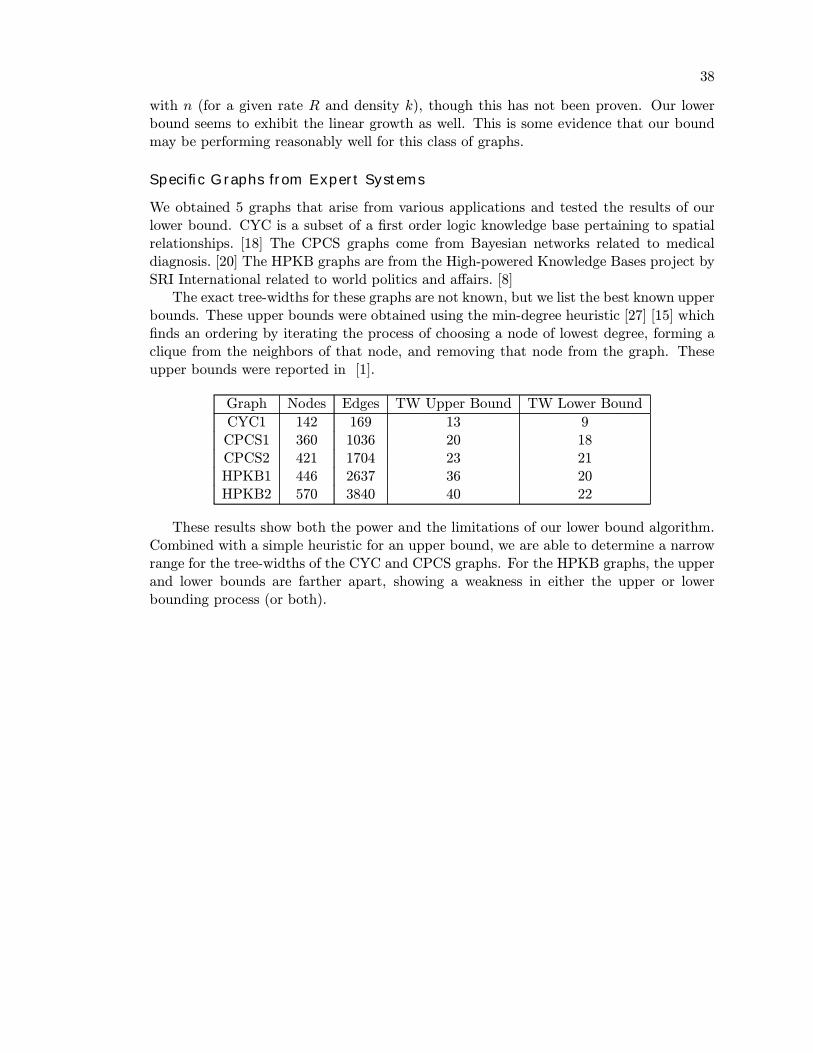
38

with n (for a given rate R and density k), though this has not been proven. Our lowerbound seems to exhibit the linear growth as well. This is some evidence that our boundmay be performing reasonably well for this class of graphs.

Specific Graphs from Expert Systems

We obtained 5 graphs that arise from various applications and tested the results of ourlower bound. CYC is a subset of a Þrst order logic knowledge base pertaining to spatialrelationships. [18] The CPCS graphs come from Bayesian networks related to medicaldiagnosis. [20] The HPKB graphs are from the High-powered Knowledge Bases project bySRI International related to world politics and affairs. [8]

The exact tree-widths for these graphs are not known, but we list the best known upperbounds. These upper bounds were obtained using the min-degree heuristic [27] [15] whichÞnds an ordering by iterating the process of choosing a node of lowest degree, forming aclique from the neighbors of that node, and removing that node from the graph. Theseupper bounds were reported in [1].

Graph Nodes Edges TW Upper Bound TW Lower Bound

CYC1 142 169 13 9CPCS1 360 1036 20 18CPCS2 421 1704 23 21HPKB1 446 2637 36 20HPKB2 570 3840 40 22

These results show both the power and the limitations of our lower bound algorithm.Combined with a simple heuristic for an upper bound, we are able to determine a narrowrange for the tree-widths of the CYC and CPCS graphs. For the HPKB graphs, the upperand lower bounds are farther apart, showing a weakness in either the upper or lowerbounding process (or both).

39

2.6 Conclusions

We have demonstrated equivalent notions of the tree-width of a graph and related theseequivalences to the computational equivalence of various methods of inference on graphicalmodels. We then proved a theroem that the maximum cardinality search procedure canbe used to get a lower bound on the tree-width of a graph. We gave simple examples toshow that this bound can be quite good or quite weak. We then suggested an algorithmwhich combines maximum cardinality search with edge contraction and wise heuristics toimprove the lower bound. This algorithm was implemented and run on lattices, LDPCgraphs, and several speciÞc graphs from expert systems. The bounds on the lattices werequite weak, but on graphs used in practice, the bound seemed to perform well. In acouple of cases, the lower bound was within 2 of known upper bounds to the tree-width ofthe graph. This suggests that practioners of inference on graphical models may Þnd thisbound to be a useful tool.

Chapter 3

Complexity Results andApplications for Coarse-to-FineDynamic Programming

40

41

3.1 Introduction

The previous chapter dealt with issues of complexity that arise from Markov RandomÞelds. We saw the limitations of computing on graphs using standard Dynamic Program-ming techniques and other equivalent methods. These methods are feasible as long asthe tree-width of the underlying graph and the state space at each node is not too large.Precisely, the computational time required is O(n|S|k+1), where n is the number of nodes,S is the state space at each node, and k is the tree-width of the underlying graph. Inpractical applications, the linear dependence on n is rarely a problem, but a large k ren-ders many problems infeasible, as we saw in the previous chapter. Even if k = 1 a hugestate space can cause |S|2 to be computationally intractable. This is the case with manyof the speech recognition systems based on Hidden Markov Models.

Coarse-To-Fine Dynamic Programming (CFDP) is a variation on DP that can be usedin various kinds of optimization problems [22]. SpeciÞcally, it is applicable to Þnding themost likely conÞguration on a Markov random Þeld, and has also been used to numericallysolve some calculus of variations problems. In the MRF setting, the idea is that when thestate space is large, rather than examine each state individually, we group the states intolarge groups called superstates. We then deÞne a new MRF using efficiently computableupper bounds for the values of the clique functions across the various state combinationsin our superstates. By using standard DP, we Þnd the most likely superstate conÞgurationon this new MRF, and since the state space is small, it will run efficiently. We then usethe result of this DP step to make a more �reÞned� graph. That is, we break some ofthe superstates into smaller groups and iterate DP again. The surprising fact is thatthis can be done in a way so that we Þnd the exact most likely conÞguration. The catchis that the speed of CFDP depends on the structure of the grouping and the nature ofthe problem. In the best case, CFDP yields a large computational savings over standardDP; in the worst case, it will actually be slower. Furthermore, to implement CFDP, wemust be able to efficiently compute a maximum of the clique functions over a subset ofstates. CFDP has been effectively used in problems from image processing [23], calculusof variations [22], and algebraic coding theory [16].

3.2 Explanation of the method

Before giving a rigorous deÞnition of CFDP, we will demonstrate its use on a simpleexample. In Figure 3.1 we are given a Markov random Þeld with respect to a simple chaingraph. Below it, we have a trellis where each column of nodes represents the different statepossibilites for the random variables in the Markov random Þeld. As usual, we assume,for the sake of simplicity, that all 5 variables X1, X2, . . . , X5 take values in the same setS. We have a probability function P deÞned on X = (X1,X2,X3, X4, X5). We want toÞnd the most likely conÞguration of this Markov random Þeld, that is to Þnd:

x$ = argmaxx∈S5

P (x) (3.2.3.1)

One canonical problem that is solved by dynamic programming is to Þnd the �maxi-mum path� across a trellis. Suppose we are given a trellis such as the one in Figure 3.1and each of the edges is given a certain value. Using DP, we can efficiently Þnd the pathfrom the leftmost column to the rightmost column which maximizes the sum of the edge

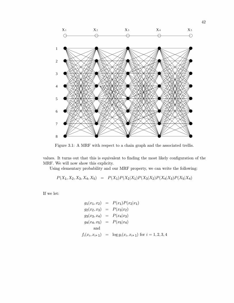
42

���

���

���

���

����

����

���

���

����

���

���

���

���

���

���

���

���

����

����

���

���

����

���

���

���

���

���

���

���

���

����

����

���

���

����

���

���

���

���

���

���

���

���

����

����

���

���

����

���

���

���

���

X 1 X 2 X 3 X 4 X 5

������

������

������

������

��������

��������

������

������

��������

������

������

������

������

1

2

3

4

5

6

7

8

Figure 3.1: A MRF with respect to a chain graph and the associated trellis.

values. It turns out that this is equivalent to Þnding the most likely conÞguration of theMRF. We will now show this explicity.

Using elementary probability and our MRF property, we can write the following:

P (X1,X2,X3,X4,X5) = P (X1)P (X2|X1)P (X3|X2)P (X4|X3)P (X5|X4)

If we let:

g1(x1, x2) = P (x1)P (x2|x1)

g2(x2, x3) = P (x3|x2)

g3(x3, x4) = P (x4|x3)

g4(x4, x5) = P (x5|x4)

and

fi(xi, xi+1) = log gi(xi, xi+1) for i = 1, 2, 3, 4

43

we can write:

x$ = argmaxx∈S5

P (x)

= argmaxx∈S5

logP (x)

= argmaxx∈S5

log

4!i=1

gi(xi, xi+1)

= argmaxx∈S5

4#i=1

log gi(xi, xi+1)

= argmaxx∈S5

4#i=1

fi(xi, xi+1)

So if we label the edge from node j in column i to node k in column i + 1 with thevalue fi(j, k) then the maximum path corresponds to the most likely conÞguration underthe distribution P .

Solving this problem is a straightforward application of standard DP. For each nodein the second column, we consider every node in the Þrst column. At every node in thesecond column, we store the node in the Þrst column which gives the best path to thesecond column, and the value of the path to that point. We then move to the third column,and for each node there, consider which node in the second column leads to the best path.Given the second column, the best choice for the third column is independent of the Þrstcolumn so we need not look back further. We continue this process until we completethe last column. At this point we examine every node in the last column to see whichending point gives the highest value. We then backtrack from that node using our storedinformation to Þnd the path which led to this highest value. The number of operationsthis requires is (n− 1)S2.

Suppose, however, that for any pair of groups of nodes in neighboring columns, wecould quickly get the value of the edge of highest value between any two nodes in the twogroups. In other words, in our problem we can Þnd:

maxj∈S1⊂S;k∈S2⊂S

fi(j, k) (3.2.3.2)

without having to actually examine every single one of the |S1| × |S2| possibilities. Wecould then use the following procedure to Þnd the maximum path across the trellis. First,we split the nodes in each column into two groups called �superstates�. We then putedges between these superstates and label them with the maximum value of all of theedges connecting any of the nodes contained in the superstates. We then iterate standardDP on this superstate graph, to Þnd the best path across this �optimistic� graph. Thevalue of a path in this superstate trellis is just an upper bound on the value of any singlenode path through nodes contained in those superstates. So the best path through thesuperstate trellis is just the region of the original trellis with the best upper bound, usingthe overestimates deÞned by the current superstate trellis. We then �reÞne� along thisbest path. That is, the superstates that were on this �best� path are divided into twosmaller superstates. Now a new graph is formed where each column has 3 superstatesinstead of 2. We repeat this process of Þnding paths and reÞning until we Þnd a path

44

which is composed entirely of single nodes (once a superstate is divided into single nodesit is divided no further). At that point we have found the best path through the entireoriginal graph, since the value of our single node path is higher than upper bounds for allother possible paths. This process is illustrated in Figure 3.2.

Although we are guaranteed to Þnd the best path through the graph eventually, wehave no guarantee in general that we will save time in this process. For example, if theentire graph must be divided into individual nodes before the algorithm terminates, wehave spent a great deal of time just to perform standard DP on the original graph asour Þnal step. However, if large chunks of the trellis remain unreÞned, we will save time.This is because we avoid examining every possibility in those sections of the trellis. Inthe best case, we never choose a path of superstates that does not contain the true bestpath. In that case, we would iterate standard DP (logS) times and the most expensive ofthese iterations would take (n− 1)(logS)2 operations. So our computational time will beO(n(logS)3) which is considerably less than nS2. In the worst case, we iterate DP O(S)times, the most expensive of which costs nS2, giving a time complexity which is O(nS3),which is clearly worse than nS2.

45

���

���

���

���

���

���

���

���

������

������

������

������

������

������

������

������

������

������

������

������

������

������

������

������

���

���

���

���

���

���

���

���

���

���

���

���

���

���

���

���

���

���

���

���

���

���

���

���

100

100

60 60

����

����

����

����

����

����

����

����

����

����

����

����

����

����

����

����

��������

��������

��������

��������

��������

��������

��������

��������

������������

����������

100

100

60 60

60 60

100

100

(c) (d)

100 100

60 60

(b)(a)

Figure 3.2: Four trellises in various stages of the CFDP process. Dotted edges representedges with a value of 0.

46

3.3 Continuous Framework

We would like to know when CFDP will save time over standard DP. From a theoreticalperspective, we would like to have sufficient conditions, which if met, would ensure aspeciÞc time complexity for CFDP which is signiÞcantly less than the time complexity ofstandard DP for the same problem. Such a theoretical result would yield insight on thetypes of problems for which CFDP would be a practical method.

The key to the efficiency of CFDP is that the coarse graph must reveal somethingabout the true best path across the trellis. CFDP will save time if there are large areasof the trellis which remain at a coarse resolution. So rather than explore each and everyone of these �bad� possibilities, CFDP is able to dismiss them all very quickly. However,CFDP can easily be fooled into searching and resolving an area of the trellis which has,in fact, no good path. Consider using CFDP on the trellis in Figure 3.2(a). On the Þrstiteration it chooses the path across the top half of the trellis, since the optimistic estimateis higher there, as illustrated in part (b) of the Þgure. The value of the top path in thecoarse graph is 200. After it reÞnes along that top path we have the trellis shown inpart(c). We Þnd that the two 100 value edges do not actually connect, and the price toswitch one of them turns out to be quite large. After part (c) we choose the bottommostpath across the trellis, and reÞne those superstates so that in part (d) we are back to ouroriginal trellis conÞguration, having completely reÞned all our superstates.

This example is trivial in the sense that we only have 4 nodes in each column andcould not expect CFDP to yield much of a savings to begin with. However, it highlights asituation where CFDP may run into trouble. We might expect CFDP to perform betterif the nodes that were grouped together were similar in some sense. To be more precise,suppose there were some notion of �distance� between nodes and that edges betweennearby nodes were close in value. Examining again the situation in Figure 3.2 we see thata problem arises because two edges from the same nodes to �nearby� nodes (that is, nodesthat are grouped together as long as possible) have drastically different values, namely 100and 0. Thus we have no guarantee that the result at the coarse resolution has anythingto do with the true best path. However, if we knew, for example, that the edge valuescould not differ very much between �nearby edges� (i.e. edges connecting �nearby� nodes)we could be sure that there is a true path somewhat close in value to the �optimistic�estimate.

This is all very intuitive and informal. To make this into a mathematically preciseframework, we consider a continuous analog to our generally discrete framework. Tobegin we choose a maximum resolution R = 2p for some positive integer p. As R getsbigger, we are more closely approximating the true continuous problem. We choose R as adyadic number since we are using a binary splitting rule (i.e. we divide our superstates inhalf). In this setting, our discrete columns of nodes are represented by the interval [0, 1],individual nodes, correspond to intervals of some minimum length l = 1

R and superstatesare represented by intervals of a longer length. The edge values between nodes and/orsuperstates correspond to the maximum of a function f over the intervals. In this way,we have a natural notion of distance between nodes. Furthermore, by putting conditionson our function f we can ensure that if two pairs of nodes are �near� to each other thenthe edges connecting those pairs of nodes will also be close in value. This setting enablesus to make precise statements about the run time of CFDP under certain conditions ofthe function f . Continuing the correspondence, paths of superstates will correspond to�rectangles� in [0, 1]n, while paths of single states will be rectangles of minimum length.

47

This will be made precise shortly.In this paper, we will concern ourselves with how the CFDP run time grows with R.

The results are of an asymptotic nature (for R �big enough�). For this reason, we willtake n to be a constant of the problem and ignore the dependence of the run time on n.This is reasonable since the issue of large state space or tree width is typically the moreimportant computational issue than the number of nodes in the graph.

3.3.1 Definitions and Notation

We state precisely many deÞnitions that will be required to perform this mathematicalanalysis. It is useful to keep in mind the correspondences stated in the previous paragraph.For the time being we will restrict ourselves to only simple chain graphs. Later in the paperwe will extend these results to general graph structures. This section is very technical,yet this is necessary to create a mathematical framework under which precise statementscan be proven.

Most of the mathematics in this paper will take place on the space [0, 1]n. In generalwe will use lowercase letters with a bar over them, such as x to refer to points in [0, 1]n.So x = (x1, x2, . . . xn). An uppercase letter with a bar over it, such as I will refer toa �rectangle� in [0, 1]n. For example, I = (I1, I2, . . . , In) where Ij = [aj, bj], a closedinterval in [0, 1]. The n dimensions of our space may be referred to as coordinates, andwill usually be indexed by the letter j.

Proceeding with the continuous formalism, we specify a function f

f : [0, 1]n −→ IR (3.3.3.1)

We assume this function respects our chain graph structure. That is, we assume

f(x) = f1(x1, x2) + f2(x2, x3) + . . .+ fn−1(xn−1, xn) (3.3.3.2)

where the fj are functions from [0, 1]× [0, 1] −→ IR.With some abuse of notation, we can extend the functions f, fj to accept rectangles

in the following way. First let

fj(Ij , Ij+1) = supxj∈Ij ;xj+1∈Ij+1

fj(xj , xj+1) (3.3.3.3)

Then

f(I) = f1(I1, I2) + f2(I2, I3) + . . .+ fn−1(In−1, In) (3.3.3.4)

Recall that rectangles will represent paths through our trellis. It will be important toquantify the size of a rectangle. We denote the length of an interval Ij by m(Ij). For ourpurposes, it is most convenient to classify the size of a rectangle by the size of its largestdimension.

Definition 3.3.1. We deÞne the size of a rectangle I by

|I| = maxjm(Ij) (3.3.3.5)

If |I | = l(= 1R) then I is a rectangle which represents a choice of a single state for each

variable.

48

Definition 3.3.2. Let the set of minimum length rectanglesM =M(R) be the set of allsuch rectangles. More precisely,

I ∈M(R)⇐⇒ Ij =

'cj − 1R

,cjR

((3.3.3.6)

where cj is an integer in 1, 2, . . . R for all j = 1, 2, . . . , n.

For simplicity we assume a unique point maximum x∗ of f and that (for R big enough)there exists a unique I∗(R) ∈M(R) which maximizes f(I) over all I ∈M(R). 1

Then the solution to our continuous problem can be restated as Þnding

I∗(R) = arg maxI∈M(R)

f(I) (3.3.3.7)

where I∗ is the unique solution to the problem.Let us review how our continuous formulation leads to a discrete graph trellis. We

specify set of functions f, fj as in Equation 3.3.3.2. We then specify the maximum resolu-tion R = 2p for some positive integer p, which implies that our minimum length intervalswill be of size l = 1

R . We then represent each minimum length interval as a node, and letthe edge between minimum length intervals in adjacent columns j and j + 1 be given bythe maximum of the function fj over every possible pair of points in those two intervals.In this way, we have a trellis, and can use standard DP or CFDP to Þnd our answer. Forevery value of R we have a different trellis, with more nodes as R increases. The questionis, how does our run time increase with R. We know that using standard DP, our run timewill grow like R2. How will the CFDP run time grow as we increase R? That questionwill be answered in this paper, under certain conditions for the functions fj .

So far, we have deÞned precisely the continuous analogs to states, superstates, columnsof nodes, and edge values. We still need to have a representation for the pattern of ourtrellis. That is, which superstates exist in which columns at a given iteration of CFDP.To do this, we introduce the notions of interval partitions, interval decompositions andresolution patterns.

Definition 3.3.3. An interval partition P is an ordered set of numbers in the interval[0, 1]; P = {a1, a2, . . . , ak} with 0 < ai < ai+1 and ak = 1. DeÞne the correspondinginterval decomposition P $ to be the set of k intervals {[0, a1], [a1, a2], . . . , [ak−1, 1]}.

The difference between the interval partition and interval decomposition is somewhatsemantic. The Þrst is a set of points while the second is a set of intervals.

Definition 3.3.4. A resolution pattern P is a set of n interval partitions; one for eachcoordinate. P = (P1, P2, . . . , Pn)

We will also deÞne inclusion operations between resolution pattern.

Definition 3.3.5. We will say P∗ ⊂ P if P ∗j ⊂ P ∗j for j = 1, 2, . . . , n. Another way ofsaying this is that P is more reÞned than P∗.

1This assumption avoids the problems that we face when the true point maximum is a dyadic point(e.g. x∗j = 3

4for all j). When that happens, we often have a singular situation where the rectangles I1,a

(defined by I1,aj = [ 3

4 − 12a , 3

4 ] for all j) and I2,a defined by I2,aj = [ 3

4 , 34 + 1

2a ] for all j) are such that

f(I1,a) = f(I2,a) for all a and there is not a unique I∗ for any R. We make this assumption to avoiddealing with such details.

49

For our purposes, it is most convenient to judge the size of a resolution pattern bythe size of its largest interval partition. In this way we can use the size of the resolutionpattern to bound the complexity of a DP iteration on that pattern.

Definition 3.3.6. The size of a resolution pattern P , denoted |P| will be given by

|P| = maxj|Pj| (3.3.3.8)

Definition 3.3.7. The basic resolution pattern Pb is the pattern given by Pj = {12 , 1} for

all j.

Definition 3.3.8. For any resolution pattern P deÞne the corresponding set of availablerectangles A(P) in the following way:

I ∈ A⇐⇒ Ij ∈ P $j for j = 1, 2, . . . , n

So A represents all the possible paths through the graph at the current state of reso-lution.

We can now state the CFDP procedure in a mathematically precise manner. Given thefj , f , a starting resolution pattern P1, and R; CFDP uses the following two-step iterativeprocess to Þnd I∗. First CFDP Þnds

I i = arg maxI∈A(Pi)

f(I) (3.3.3.9)

through standard dynamic programming. Here we are not necessarily guaranteed a uniqueanswer, so we just break ties arbitrarily. If Ii ∈ M(R) then the algorithm stops andoutputs I∗ = Ii. Otherwise the resolution pattern Pi+1 is formed by adding the midpointof Iij to P

ij for all j such that m(I

ij) > l. This procedure then repeats until an answer is

found.

Lemma 3.3.9. If Ii = argmaxI∈A(Pi) f(I) and Ii ∈M(R) then:

Ii = I∗ = arg maxI∈M(R)

f(I) (3.3.3.10)

Proof. Take any I ∈M(R). There exists a I $ ∈ A(P i) such that I ⊆ I $. Therefore f(I $) ≥f(I). Furthermore, f(Ii) ≥ f(I $) since Ii is the argmaxI∈A(Pi) f(I). Therefore f(Ii) ≥f(I) for all I ∈M(R). Therefore, it must be the case that I = I∗ = argmaxI∈M(R) f(I).

We can speak of running CFDP to completion, that is until CFDP Þnds I∗, or wecan just run CFDP for a Þxed number of iterations and analyze Ii and P i. We can alsospecify no minimum length and have CFDP output an inÞnite sequence of rectangles Ii.

Note that the resolution patterns created by CFDP have a certain structure. Let P bethe resolution pattern resulting from some number of iterations of CFDP on some problemwith the initial resolution pattern Pb (the basic resolution pattern deÞned above). Forexample, consider a particular Pj. If

38 ∈ Pj then 1

2 ,14 ∈ Pj as well. This is a result of

the coarse-to-Þne progression of our intervals. If 38 is in Pj, that means that the interval

50

_12

_ _

__ _ _

_ _ _ _ _ _ ___ __ __________

����

����

����

����

����

����

����

����

����

����

����

����

����

����

����

14

34

1

1

8

16

8 8 8753

16 16 16 16 16 16 163 5 7 9 151311

Figure 3.3: The �legality� tree of height 4.

[ 14 ,12 ] must have been chosen by CFDP, which implies that those points must have been

in the interval partition already. In general, for any xj ∈ Pj , xj ,= 0, 1 we can writexj =

2mcoR for some odd integer co. If P is a resolution pattern created by CFDP from the

basic resolution pattern, then Pj will have the following property: if xj =2mcoR ∈ Pj then

2m(co−1)R , 2m(co+1)

R ∈ Pj. We will now make this deÞnition explicit.Definition 3.3.10. A resolution pattern P is said to be legal if for all j = 1, 2, . . . , n wehave that if 2mco

R ∈ Pj for some odd integer co then 2m(co−1)R , 2m(co+1)

R ∈ Pj.Another way to understand legality is to consider the tree in Figure 3.3, where each

node is identiÞed with a number. The legality requirement is equivalent to saying that ifsome number is in Pj than all its ancestors on the �legality� tree must be as well.

Definition 3.3.11. Let I $ = argmaxI∈A(P) f(I). A resolution pattern P is said to be

sufficient for a particular problem at a particular resolution R, if I $ ∈M(R).

Note that by Lemma 3.3.9 we can conclude that if P is sufficient, then:

I $ = arg maxI∈A(P)

f(I) = arg maxI∈M(R)

= I∗ (3.3.3.11)

We can already begin to prove a few basic lemmas about these objects we have deÞned.

Lemma 3.3.12. Fix a maximum resolution R. Given two resolution patterns, P1 andP2, if P1 is more reÞned than P2 (i.e. P 2

j ⊆ P 1j for all j), and P2 is sufficient, then we

have that P1 is sufficient.

Proof. Since P2 is sufficient, we know that I∗ ∈ A(P2). Since, by deÞnition I∗ ∈M(R)we know that I∗ ∈ A(P1). So all we need to show is that given any other I ∈ A(P1),I ,= I∗, we have that f(I∗) > f(I). Suppose, by contradiction, we had an I ∈ A(P1),I ,= I∗ such that f(I) ≥ f(I∗). There must exist some I2 ∈ A(P2) such that I ⊆ I2.Therefore f(I2) ≥ f(I) ≥ f(I∗) which contradicts the sufficiency of P2.

Lemma 3.3.13. Let I1, I2, . . . be a sequence of rectangles chosen by CFDP. Then for alli, f(Ii) ≥ f(Ii+1) and f(Ii) ≥ f(I∗) ≥ f(x∗).

51

Proof. Consider Ii+1 = (Ii+11 , Ii+1

2 , . . . , I i+1n ). There exists some I = (I1, I2, . . . , In) in

A(P i) such that Ii+1j ⊆ Ij for all j. Therefore f(I) ≥ f(Ii+1), since each maximum is

taken over at least as big a set in I as it is in Ii+1. But we know that f(I i) ≥ f(I) sinceI i is the arg max over the set A(P i). Therefore f(Ii) ≥ f(Ii+1). Since I∗ is the result ofthe last iteration, it follows that f(I i) ≥ f(I∗).

We know that there exists I ∈ M such that x∗ ∈ I. By deÞnition of f on intervalsf(I) ≥ f(x∗). It then follows that f(I∗) ≥ f(I) by deÞnition of arg max.

Suppose that we specify no minimum length and run CFDP to get an inÞnite sequenceof rectangles Ii. It is shown in [22] that if the fj are continuous, then I

i converges to x∗

in the sense that if xi is any sequence of points satisfying xi ∈ Ii then xi → x∗.

3.3.2 Main results (chain graph)

Our goal is to give a limit on the CFDP run time for a particular problem; that is, aparticular set of fj . Here are the two main results we prove for the 1-dimensional �chaingraph� setting. They show that, in our continuous framework, we realize a tremendouscomputational savings when the fj are linear, and a considerable savings when the fj�look quadratic� around the maximum of f . Furthermore, these results are tight. Thatis, there exists problems which meet our assumptions which require the same order ofcomputation that we give as an upper bound.

Theorem 3.3.14. Suppose the fj are continuous and piecewise linear, f has a uniquepoint maximum x∗, and there exists some R1 such that R > R1 implies I

∗ is unique. Thencoarse-to-Þne dynamic programming will Þnd the rectangle I∗(R) in time O((logR)3).

Theorem 3.3.15. Suppose the fj are C2 and that f has a unique maximum x∗. Assume

further that the Taylor expansion of f at x∗ has a negative-deÞnite matrix coefficient inthe quadratic term. Finally, assume there exists some R1 such that R > R1 implies I

∗ isunique. Then coarse-to-Þne dynamic programming will Þnd the rectangle I∗(R) in timeO(R

32 ).

The proofs to these theorems (in a more general form) are in the Appendix. For nowwe will just make a few remarks:

1. These bounds are both tight with respect to R. That is, there are fj that arepiecewise linear that require at least K(logR)3 operations and fj that meet the

conditions of Theorem 3.3.15 which require at least KR32 operations. The tightness

in the piecewise linear case is apparent since even if CFDP is perfect (i.e. onlychooses the superstates which contain the true solution), it will take (logR)3 (pluslower order terms) operations. The tightness for the C2 case can be easily con-Þrmed analytically in simple cases, take, for example, when n = 3, f1(x1, x2) =x1+x

22+4x2, f2(x2, x3) = −(5

2)x22−2x2+x3. So x

∗1, x

∗3 = 1 and the only interesting

aspect of the problem is the behavior of x2. In this case, elementary calculus canshow that any sufficient resolution pattern P must have |P2| > K

√R. This becomes

clearer after reading the proof.

52

2. In practical examples, we are often unable to compute:

fj(Ij, Ij+1) = supxj∈Ij ;xj+1∈Ij+1

fj(xj, xj+1) (3.3.3.12)

exactly. Instead we settle for Þnding heuristics hj:

hj(Ij, Ij+1) ≥ supxj∈Ij ;xj+1∈Ij+1

fj(xj, xj+1) (3.3.3.13)

and deÞne

h(I) = h1(I1, I2) + h2(I2, I3) + . . .+ hn−1(In−1, In) (3.3.3.14)

As long as h(I)− f(I) ≤ K|I| for some constant K and h(I) = f(I) for I ∈M(R),then the results of our theorems still hold when using CFDP on the hj to Þnd themaximum for f .

3. Our setup for CFDP has been geared towards Þnding maxima. An analogous pro-cedure can be used to Þnd minima instead.

4. We see that in the linear case we get quite a large savings over standard DP � fromO(R2) to O((logR)3).For the general C2 case, we get considerable savings, O(R

32 )

versus R2. This is potentially a huge savings. Suppose we have a problem wherewe want R ≈ 106 ≈ 220. For standard dynamic programming we would need 1012

operations, that is, a trillion operations. If the problem is piecewise linear, usingCFDP we perform the same computation in about 8,000 operations (using log2). Ifthe problem is just C2, we still cut the computation to 109 operations, from a trilliondown to a billion.

53

3.4 Example — the isoperimetric problem

To illustrate this computational savings in a 1-D setting, we consider a simple calculus ofvariations problem: the so-called �isoperimetric� problem. The problem is; given a curveof a Þxed length, starting at the origin and ending somewhere on the positive x-axis, toenclose the largest area possible between the curve and the x-axis. The answer is simple� a semicircle.

We formulate this as a continuous trellis problem in the following way. We Þx thelength of our curve, and divide it up into n equal pieces and we let yj represent the heightof the curve above the x-axis after j segments. We form a trellis with n + 1 columns ofnodes, numbering them from 0 to n. Column 0 and column n each have only one point,corresponding to the fact that we must start and end on the x-axis. We can think of thesecolumns as being represented by the interval [0, 0]. Columns 1 and n − 1 are representedby the interval [0, 1]. Since clearly it is inefficient to go below the x-axis, we consider onlycurves that stay above the axis. Since our segments are of unit length, the highest we couldpossibly be right after the Þrst segment (or right before the last segment) is 1. Followingthis logic, columns 2 and n − 2 are respresented by the interval [0, 2] and in general, forj = 0, 1, 2, . . . 2n2 3, we represent columns j and n − j by the interval [0, j]. This differsslightly from the setup in our theorem, where every column of nodes was represented byan equally sized interval, but it is easy to see the the result of Theorem 3.3.14 is still inforce.

Note that our progression in the direction of the x-axis (i.e. away from the y-axis) isconstrained by our choices of the yj, since our segments are of unit length. In other words,consider this problem for n = 6 and consider the path given by y0 = 0, y1 = 1, y2 = 2, y3 =3, y4 = 2, y5 = 1, y6 = 0. This path through our trellis corresponds to a curve which goesstraight up from the origin to the point (0, 3) and then straight back down to the origin,enclosing no area. This is because our segments are of length 1 and therefore if we increaseour height (i.e. y-coordinate) by 1 then we do not increase our x-coordinate at all. The

path given by y0 = 0, y1 =√

22 , y2 =

√2, y3 =

3√

22 , y4 =

√2, y5 =

√2

2 , y6 = 0 corresponds

to a curve consisting of two linear segments, the Þrst from the origin to ( 3√

22 , 3

√2

2 ), and

the second from ( 3√

22 , 3

√2

2 ) to (3√2, 0). This curve encloses an area of size 9

2 .We need to deÞne our functions f and fj to reßect this area function. The value of

an edge between columns j and j + 1 should correspond to the area enclosed under thatsegment (see Figure 3.4). Using simple geometry, our function fj is given by:

fj(yj , yj+1) =

)((yj + yj+1)/2)

*(1− (yj − yj+1)2) if |yj − yj+1| ≤ 1,

−∞ otherwise.(3.4.3.1)

Here the root term represents the width of the trapezoidal region we are considering andÞrst term represents the �average� height. We let f(yj , yj+1) = −∞ when |yj − yj+1| > 1since it is impossible to change the height by more than 1 between the start and end of asegment.

So if we let:

f(y) = f(y0, y1, . . . , yn) =

n−1#j=0

fj(yj, yj+1) (3.4.3.2)

54

yi

yi

yi+1

yi+1

−yi+1 yi1 − ( )2

���������������������������������������

���������������������������������������

−| |

Figure 3.4: The area enclosed by one segment.

then we are looking for y∗ such that

f(y∗) = supy∈D

f(y) (3.4.3.3)

where the domain D is deÞned by yj, yn−j ∈ [0, j] for j = 0, 1, 2, . . . , 2n2 3. Since thedomain is compact we know the sup is achieved and y is continuous.

Now that we have deÞned precisely the mathematical problem and shown how it trans-lates into Þnding the maximum path on a �continuous� trellis, the coarse-to-Þne approachshould be fairly straightforward. We deÞne a resolution R = 2b for some integer b and letour minimum length l be given by l = 1

R . So given R we have a discrete trellis, where thenodes represent intervals of length l and the edge value between two intervals is given by:

fj(Ij , Ij+1) = supyj∈Ij ;yj+1∈Ij+1

fj(yj , yj+1) (3.4.3.4)

Recall that a key practical requirement for implementation of CFDP is that we canefficiently compute the maximum of a function over all the individual state combinationsin a superstate. For our problem, this amounts to being able to efficiently computefj(Ij, Ij+1). Fortunately, there is an efficient way to compute this.

It is important Þrst to notice we need only consider yj, yj+1 pairs where at least one ofthe two is the highest value in its interval. We make this precise in the following lemma.

Lemma 3.4.1. Let Ij = [aj , bj ], Ij+1 = [aj+1, bj+1] and (yj, yj+1) ∈ Ij × Ij+1. Thereexists (y$j , y$j+1) ∈ Ij × Ij+1 such that f(y

$j, y

$j+1) ≥ f(yj , yj+1) and either y

$j = bj or

y$j+1 = bj+1.

Proof. Choose yj < bj and yj+1 < bj+1. If |yj − yj+1| > 1 then f(yj , yj+1) = −∞ andthe lemma is trivial, so assume |yj − yj+1| ≤ 1. Let $ = min{bj − yj , bj+1 − yj+1} and let

55

y$j = yj + $ and y$j+1 = yj+1 + $. We know that:

f(y$j , y$j+1) =

+y$j + y

$j+1

2

,-1− (y$j − y$j+1)

2

=

+yj + yj+1 + 2$

2

,-1− (yj − yj+1)2

=

+yj + yj+1

2

,-1− (yj − yj+1)2 + $

-1− (yj − yj+1)2

> f(yj, yj+1)

So we can use the following process to compute fj(Ij, Ij+1). Letting Ij = [aj, bj], Ij+1 =[aj+1, bj+1], we compute:

supyj+1∈Ij+1

fj(bj, yj+1)

and

supyj∈Ij

fj(yj , bj+1)

and then choose the larger of those two values.Using simple calculus, we can compute that f(bj , yj+1), viewed as a function of yj+1

only, achieves its maximum at yj+1 =bj2 +

bj2

-1 + 2

b2j(if bj = 0, yj+1 =

√2

2 ). Furthermore,

this is the only critical point of that function in the range yj+1 = [bj − 1, bj +1]. Since fjis symmetric in its two arguments, this analysis also applies to the case where yj+1 = bj+1

and fj is a viewed as a function of yj only.So to compute supyj+1∈Ij+1

fj(bj, yj+1), we just let

y∗j+1 =

bj2 +

bj2

-1 + 2

b2j

ifbj2 +

bj2

-1 + 2

b2j∈ Ij+1,

bj+1 ifbj2 +

bj2

-1 + 2

b2j> bj+1.

aj+1 ifbj2 +

bj2

-1 + 2

b2j< aj+1.

(3.4.3.5)

Then:

supyj+1∈Ij+1

fj(bj, yj+1) = fj(bj, y∗j+1) (3.4.3.6)

Analogously we let:

y∗j =

bj+1

2 +bj+1

2

-1 + 2

b2j+1

ifbj+1

2 +bj+1

2

-1 + 2

b2j+1

∈ Ij,bj if

bj+1

2 +bj+1

2

-1 + 2

b2j+1

> bj.

aj ifbj+1

2 +bj+1

2

-1 + 2

b2j+1

< aj.

(3.4.3.7)

56

........

........

........

........

........

........

........

........

........

........

........

........

........

........

........

........

........

........

........

........

Figure 3.5: The initial trellis for the isoperimetric problem with n = 8 and R = 8.

so that:

supyj∈Ij

fj(bj, yj+1) = fj(y∗j , bj+1) (3.4.3.8)

Then by Lemma 3.4.1 we know that:

fj(Ij , Ij+1) = supyj∈Ij ;yj+1∈Ij+1

fj(yj , yj+1) = max{fj(bj , y∗j+1), fj(y∗j , bj+1)} (3.4.3.9)

In this way, we can efficiently compute fj(Ij , Ij+1) and thereby implement CFDP.We have now demonstrated that we have all the tools necessary to use CFDP to solve

this problem. We select a value R = 2b for some integer b to be our resolution. Forsimplicity, we choose our starting resolution pattern Ps to be deÞned by:

Psj ,Psn−j = {1, 2, . . . , j} for j = 0, 1, 2, . . .2n2

3In other words, we start with a resolution pattern where each interval is divided into piecesof length 1. This is shown in Figure 3.5.

3.4.1 Empirical results

We implemented a CFDP solution to this discretized version of the isoperimetric prob-lem using MATLAB. In this way we are able to observe directly how the number ofoperations increases with R. This allows us to conÞrm experimentally the predictions ofTheorem 3.3.15. The function f for this problem meets the conditions of the theoremexcept for the discontinuity when the fj sharply drop to −∞. However, in the proof ofTheorem 3.3.15, we see that the continuity of the f, fj is only necessary within a neigh-borhood of the maximum. Therefore, we expect to see the behaviour predicted by thetheorem.

In Figure 3.6 we see the number of operations taken by CFDP, divided by R32 , plotted

against R. If the number of operations grows like R32 , then we would expect to see the

normalized operations behave like a constant with respect to R. This appears to be exactlythe case.

57

0 500 1000 1500 2000 25001400

1500

1600

1700

1800

1900

2000

2100

2200

2300

R

(# o

f ope

ratio

ns)/

(R( 3/

2))

Figure 3.6: Our computational results for the isoperimetric problem.

58

3.5 General Graph Structures

So far, everything we have discussed has been equivalent to Dynamic Programming ona graph whose underlying structure is a simple chain. However, as we saw in the Þrstchapter, DP can be used for Markov random Þelds with an arbitrary graph structure.Instead of getting a complexity of O(R2) as in the chain graph, we get O(Rk+1) where kis the tree-width of the graph, where R is the size of the state space.

The Coarse-to-Fine Dynamic Programming method, and the continuous frameworkdescribed earlier also generalizes to the more general graph setting. To make our nota-tion work for the general setting, we must redeÞne our function f to encompass morecomplicated functions. We need to introduce cliques as subsets of {1, 2, . . . n}. Anotherdifference is that the analogy to Þnding the maximum path across a trellis is no longerstraightforward enough to be useful. Rather we must recall the generalized DP methoddiscussed in Chapter 1 and make our analogies directly to that.

Suppose we have a probability distribution P which respects (i.e. is a Markov RandomÞeld with respect to) a graph G with tree-width k. Since G has tree-width k, there existssome k-tree H such that G ⊆ H. Since P is clearly respects the graph H, without loss ofgenerality, we can just let G be a k-tree. Furthermore, we can renumber the vertices sothat the ordering π = (1, 2, 3, . . . n) has maximum border equal to k. Let C be the set ofmaximal cliques in G and let s = |C|. So we can write C in the form C = {C1, C2, . . . Cs}.Since G is a k-tree, our maximal cliques are each of size k+1. We represent a clique as asubset of {1, 2, . . . , n}. For example, we could let C1 = {1, 3, 4, 5, 7}. Given a point x welet xCi represent just the values of xj for j ∈ Ci. So writing f1(xC1) would be shorthandfor f1(x1, x3, x4, x5, x7). Likewise, given a rectangle I, we let a clique interval ICi representthe intervals Ij for j ∈ Ci.

Using this notation, we can write:

P (x1, . . . , xn) =

s!j=1

gj(xCj )

and if we let:

fj(xCj ) = log gj(xCj )

we can rewrite P in the form

logP (x1, . . . , xn) = log

s!j=1

gj(xCj )

=

s#j=1

log gj(xCj )

=

s#j=1

fj(xCj)

so that maximizing P is equivalent to maximizing the sum of the fj .So whereas in the chain graph setting we had:

f(x) = f1(x1, x2) + f2(x2, x3) + . . .+ fn−1(xn−1, xn) (3.5.3.1)

59

we have now generalized to

f(x) = f1(xC1) + f2(xC2) + . . .+ fs(xCs). (3.5.3.2)

Note that if our graph is a chain graph then the second formulation reduces to the Þrst.Continuing the generalization we have:

fj(ICj) = supxCj∈ICj

f(xCj ) (3.5.3.3)

f(I) =s#j=1

fj( ¯ICj ) (3.5.3.4)

(3.5.3.5)

From the previous chapters, we know that since f respects a graph of tree-width k,we can perform a single DP iteration on a resolution pattern P in time O(|P|k+1). Thisenables us to generalize our previous theorems to arbitrary graphs.

Theorem 3.5.1. Suppose the fj are continuous and piecewise linear, f has a unique max-imum x∗, and there exists some R1 such that R > R1 implies I

∗ is unique. Suppose furtherthat f respects a graph with tree-width k. Then coarse-to-Þne dynamic programming willÞnd the rectangle I∗(R) in time O((logR)k+2).

Theorem 3.5.2. Suppose the fj are C2 and that f has a unique maximum x∗. Assume

further that the Taylor expansion of f at x∗ has a negative-deÞnite matrix coefficient inthe quadratic term and that f respects a graph of tree-width k. Finally, assume there existssome R1 such that R > R1 implies I

∗ is unique. Then coarse-to-Þne dynamic programmingwill Þnd the rectangle I∗(R) in time O(R

k+22 ).

The proofs to these theorems are in the Appendix. Remarks 1-3 from the chain graphversions of the theorems apply to the general version as well. Note that the computationalsavings over standard DP grow considerably with the tree-width of the graph. In the k = 1case, we demonstrated savings at large R ≈ 106. If the tree-width is larger, the savingsbecome considerable even at smaller R values. Suppose R = 103 ≈ 210 and k = 4.Standard dynamic programming would require 1015 computations, out of reach by moststandards and certainly unreasonable for any kind of real-time applications. If the problemis piecewise linear, CFDP would require only 106 operations. If it is C2 CFDP would take109 operations. Both of these are tractable by today�s standards.

60

���

���

����

���

���

����

1 32

a b

c d

α

β

φγ

δ λ

η

ξ

π

µ

Figure 3.7: A spring network. Black dots are Þxed points and white dots are moveablepoints.

3.6 Multi-dimensional example

To illustrate an application of CFDP on a more complicated graph, we consider a �springnetwork� problem. This is shown in Figure 3.7. The setup is as follows. There are fourÞxed points in the plane, labeled a, b, c, d, and represented by black dots in the diagram;and three moveable points, labeled 1, 2, 3, and represented by white dots in the diagram.A total of 10 springs connect the various points. These springs are labeled by the Greekletters α,β, γ, δ,φ,π, η, ξ,λ, µ. Each spring has a resting length ls and a spring constantk. The problem is to calculate where the moveable points will come to rest in this system.One way to do this is to consider the equation for the total energy of all the springs, andÞnd the locations of the moveable points which minimize this energy. As we will soon see,this can be Þt into a generalized Dynamic Programming, and a CFDP framework.

While heretofore we have considered only maximization problems, our theorems andmethods apply analogously to minimization. The energy stored in a spring is 1

2k(ls−lact)2,where k is the spring constant, ls is the length of the spring at rest, and lact is the actuallength of the spring. Therefore, if we let, xi, yi be the x and y-coordinates of point i(for i = 1, 2, 3, a, b, c, d), and redeÞne our constants k to include the 1

2 term, then we canexpress the total energy of our system as:

f(x1, y1, x2, y2, x3, y3) = kα(lα −*(x1 − xa)2 + (y1 − ya)2)2

+kβ(lβ −*(x1 − x2)2 + (y1 − y2)2)

2 + kγ(lγ −*(x1 − xc)2 + (y1 − yc)2)2

+kδ(lδ −*(xa − x2)2 + (ya − y2)2)

2 + kφ(lφ −*(xc − x2)2 + (yc − y2)2)

2

+kπ(lπ −*(x2 − xb)2 + (y2 − yb)2)2 + kξ(lξ −

*(x2 − x3)2 + (y2 − y3)2)

2

+kη(lη −*(x2 − xd)2 + (y2 − yd)2)2 + kλ(lλ −

*(xb − x3)2 + (yb − y3)2)

2

+kµ(lµ −*(xd − x3)2 + (yd − y3)2)

2

61

��������

��������

����

����

����

����

x1 x2 x3

y1 y2 y3

Figure 3.8: The MRF dependendy graph for the spring problem.

or more simply:

f(x1, y1, x2, y2, x3, y3) = gα(x1, y1) + gβ(x1, y1, x2, y2) + gγ(x1, y1)

+gδ(x2, y2) + gφ(x2, y2) + gπ(x2, y2) + gξ(x2, y2, x3, y3)

+geta(x2, y2) + gλ(x3, y3) + gµ(x3, y3)

So if we let:

f1(x1, y1, x2, y2) = gα(x1, y1) + gβ(x1, y1, x2, y2) + gγ(x1, y1) + gδ(x2, y2) + gφ(x2, y2)

and

f2(x2, y2, x3, y3) = gπ(x2, y2) + gξ(x2, y2, x3, y3) + gη(x2, y2) + gλ(x3, y3) + gµ(x3, y3)

Then we can write:

f(x1, y1, x2, y2) = f1(x1, y1, x2, y2) + f2(x2, y2, x3, y3) (3.6.3.1)

In other words, f respects the graph G in Figure 3.8.To make this a generalized DP problem, we need to discretize the state space. We do

this, as usual, by choosing a maximum resolution R. However, in this problem there is anadditional issue to contend with. In theory, the xi and yi could be anywhere on the realline. In practice however, it is not difficult to Þnd a range in which the minimum must lie.For the purposes of our application, we consider only the interval [0, 1] for each variable.We choose the constants of our problem in a way so that this is realistic.

Once again, in order implement CFDP for this problem, we need to be able to efficientlycompute:

f1(Ix1, Iy1, Ix2, Iy2) = infx1∈Ix1 ;y1∈Iy1 ;x2∈Ix2 ;y2∈Iy2

f1(x1, y1, x2, y2)

and

f2(Ix2, Iy2, Ix3, Iy3) = infx2∈Ix2 ;y2∈Iy2 ;x3∈Ix3 ;y3∈Iy3

f3(x2, y2, x3, y3)

62

In this case, however, Þnding that inf is difficult, so we will settle instead on using aheuristic:

h1(Ix1, Iy1, Ix2, Iy2) = infx1∈Ix1 ;y1∈Iy1

gα(x1, y1) + infx1∈Ix1 ;y1∈Iy1 ;x2∈Ix2 ;y2∈Iy2

gβ(x1, y1, x2, y2) + infx1∈Ix1 ;y1∈Iy1

gγ(x1, y1) + infx2∈Ix2 ;y2∈Iy2

gδ(x2, y2)

+ infx2∈Ix2 ;y2∈Iy2

gφ(x2, y2)

≤ infx1∈Ix1 ;y1∈Iy1 ;x2∈Ix2 ;y2∈Iy2

f1(x1, y1, x2, y2)

with h2 deÞned accordingly and h = h1 + h2.We discussed earlier that our results still apply to heuristics as long as they are within

a linear factor (relative to |I|) of the true underlying function f , and are equal to f onminimum length intervals. Since f has a continuous Þrst derivative and we are working ona compact space, the Þrst condition is satisÞed. Unfortunately, we are unable to computef directly even on minimum length intervals. If we could compute f directly on minimumlength intervals, we could just deÞne h to be equal to f on minimum length intervals andtruly claim to be minimizing f . However, in this case, we are truly minimizing h and notf . However, since the difference between the two functions is linear in I, as R gets bigthis should make little difference.

To compute our heuristic h, we need to efficiently Þnd:

infx1∈Ix1 ;y1∈Iy1 ;x2∈Ix2 ;y2∈Iy2

K(l −*(x1 − x2)2 + (y1 − y2)2)

2 (3.6.3.2)

In the terms which involve only one moveable point, we just keep the Þxed point constantand take the inÞmum over the two coordinates of the moveable point.

The procedure for Þnding this inÞmum is not difficult. First we compute:

wmin = infx1∈Ix1 ;x2∈Ix2

(x1 − x2)2

and

wmax = supx1∈Ix1 ;x2∈Ix2

(x1 − x2)2

This amounts to just Þnding the inf and sup of d(x1, x2) for x1 ∈ Ix1; x2 ∈ Ix2 .Likewise we let:

zmin = infy1∈Iy1 ;y2∈Iy2

(y1 − y2)2

and

zmax = supy1∈Iy1 ;y2∈Iy2

(y1 − y2)2

If we let Iq = [√wmin + zmin,

√wmax + zmax], then

infx1∈Ix1 ;y1∈Iy1 ;x2∈Ix2 ;y2∈Iy2

K(l −*(x1 − x2)2 + (y1 − y2)2)

2 = infq∈Iq

K(l − q)2

= Kd(l, Iq)2

In this way we can quickly Þnd the required minimum and thereby implement a CFDPsolution for this problem.

63

0 100 200 300 400 500 60016

18

20

22

24

26

28

30

32

R

(# o

f ope

ratio

ns)/

(R(5

/2) )

Figure 3.9: The computational results for the spring problem.

3.6.1 Results

We implemented a CFDP solution to the spring network using MATLAB. We conÞrmedthe correctness of our answers by calculating the net force on each point in our solutionand conÞrming that it was 0 (within a reasonable error tolerance given by our intervalsize). We then analyzed how the number of operations grew with R. According to ourtheorem, we would expect asymptotically that the number of operations would grow likeR

52 . So if we scale the number of operations by dividing by R

52 we would expect that

number to behave like a constant for large enough R. In Figure 3.9 we plot the scalednumber of operations on the y-axis against R on the x-axis. While we do not see the clearconstant pattern we saw in the isoperimetric example, this is not totally unexpected. Sincethis problem requires more operations as a function of R, we were unable to increase R tothe extent we did in the previous problem. In this case, however, the improvement overstandard DP is remarkable. At R = 512, standard DP would take 2× (5122) ≈ 1.37×1011

operations. CFDP took about 1.8× 108 operations, roughly 766 times faster.

64

APPENDIX

In this Appendix we prove the main results of Chapter 3. These proofs are fairly technicalin nature, but this is necessary for mathematical precision. We will give some necessarybackground lemmas and propositions, before restating and proving our theorems. Ournotation follows from the general framework presented in Section 3.5.

Background Definitions, Lemmas, Propositions

We will use d(., .) to represent the distance function in several ways depending on thetypes of arguments. Generally, the deÞnitions are what one would expect, but we willmake them explicit here for clarity. If xj , yj ∈ IR, then:

d(xj, yj) = |xj − yj| (A-1)

We deÞne the distance between a real number xj and an interval of reals Ij by

d(xj , Ij) = infyj∈Ij

d(xj, yj) (A-2)

The distance between two points x, y ∈ IRn (or [0, 1]n) will be the simple Euclideandistance:

d(x, y) =

n#j=1

(xj − yj)2 1

2

(A-3)

Finally, the distance between a point x ∈ IRn (or [0, 1]n) and a rectangle I ⊆ IRn (or[0, 1]n) is given by:

d(x, I) = infy∈Id(x, y) (A-4)

Let the CFDP overestimate for I be given by

OE(I) = f(I)− supx∈I

f(x) (A-5)

Thus it is easy to see that if

f(x∗) > f(x) +OE(I) (A-6)

for all x ∈ I then f(x∗) > f(I).Lemma .0.1. A resolution pattern P is sufficient (for a resolution R) if for every rec-tangle I ∈ A(P) at least one of the following is true:1. I ∈M(R)

2. f(x∗) > f(I)

Proof. Let I $ = argmaxI∈A(P) f(I). For any I /∈ M(R), f(I) < f(x∗) ≤ f(I∗). SoI $ ∈M(R) and P is sufficient.

65

Proposition .0.2. Fix a set of fCj which respects a graph of tree-width k and supposethat for some sequence of resolutions R→∞ we have a legal, sufficient resolution patternP(R) = {P1(R), P2(R), . . . , Pn(R)}. If

|P(R)| = O(g(R)) (A-7)

then CFDP will run to completion in time O((g(R))k+2).

Proof. The proof of the proposition rests on the following lemma:

Lemma .0.3. Suppose we have a sufficient resolution pattern P = {P1, P2, . . . , Pn} andanother resolution pattern P1 = {P 1

1 , P12 , . . . , P

1n} which is not sufficient. Let P2 be

the resolution pattern yielded by CFDP after one iteration on the resolution pattern P1.Then there exists some number y ∈ [0, 1] and some coordinate j such that y ∈ P 2

j and

y ∈ Pj − P 1j .

Proof. Let I be the rectangle chosen on the Þrst iteration of CFDP on the resolutionpattern P1. Since P1 is not sufficient, there exists at least one j such that m(Ij) > l.Let J = {j : m(Ij) > l} and let yj =the midpoint of Ij for j ∈ J . Clearly, for j ∈ J ,yj ∈ P 2

j and yj /∈ P 1j . So we need to show that for at least one j ∈ J , yj ∈ Pj. Suppose,

by contradiction, that for all j ∈ J we have yj /∈ Pj . We will construct a rectangleI0j ∈ A(P ) in the following way. For j ∈ J , let I0

j be the interval in P$j , the interval

partition corresponding to Pj, which contains yj, so that yj ∈ I0j . Since our resolution

patterns are legal, it is not possible that I0j ⊂ Ij, so we know that Ij ⊆ I0

j .

For j /∈ J , m(Ij) = l, so let I0j be the interval in P

$j which contains Ij . By our

construction, I0 ∈ A(P ). We know that there exists a rectangle I∗ ∈ A(P ) such thatI∗ ∈ M(R) and f(I∗) > f(I) for I ∈ A(P ), I ,= I∗. We know I0 /∈ M(P ) so thereforeI∗ ,= I0. Therefore f(I∗) > f(I0). Since I ⊆ I0 we know that f(I0) ≥ f(I). Thus wehave that f(I) < f(I∗) which contradicts Lemma 3.3.13 .

Starting from the basic resolution pattern and applying the lemma repeatedly we seethat after nO(g(R)) DP iterations, if we have not already solved the problem, we will havea resolution pattern P∗ which is at least as reÞned as P . In other words, for all j, Pj ⊆ P ∗j .Since any reÞnement of a sufficient resolution pattern is itself sufficient (Lemma 3.3.12), theproblem will be solved on the next iteration. So we have used nO(g(R)) DP iterations, themost expensive of which takes time O(g(R)k+1). Thus we get a complexity of O(g(R)k+2).

Theorem for Piecewise Linear functions

Theorem .0.4. Suppose the fj are continuous and piecewise linear, f has a unique maxi-mum x∗, and there exists some R1 such that R > R1 implies I

∗ is unique. Suppose furtherthat f respects a graph with tree-width k. Then coarse-to-Þne dynamic programming willÞnd the rectangle I∗(R) in time O((logR)k+2).

Proof. All the proofs of our main results will follow this basic outline. First, we carefullydeÞne a neighborhood of x∗, called G. This region will have the property that CFDP never

66

chooses more that a constant number of rectangles outside of G, independent of R. Inother words, to determine the number of iterations required by CFDP asymptotically, weneed only consider how f behaves in the region G. We use this set G to deÞne a proceduresuch that given any �big enough� resolution R, we can deÞne a sufficient resolution patternP . We then use Proposition .0.2 to relate the size of the resolution pattern (as a functionof R) to the complexity of the problem with respect to CFDP.

We begin in the piecewise linear setting. Since f is piecewise linear, and [0, 1]n iscompact, we can Þnd a constant K1 > 0 such that:

K1 > sup{8888 ∂fi∂xj

(x)

8888 , 8888 ∂f∂xj (x)8888} (A-8)

where the max is taken over all i ∈ 1, 2, . . . s, all j ∈ 1, 2, . . . , n and all x ∈ [0, 1]n wherethe partial derivatives exist.

Lemma .0.5. Recall that we deÞned OE(I) = f(I)−supx∈I f(x). Under the assumptionsof our theorem we have:

OE(I) ≤ s(k + 1)K1|I| (A-9)

Proof. Let x$ = argmaxx∈I f(x). Using this deÞnition and expanding f we get:

OE(I) =

s#j=1

fj(ICj))− fj(x$

=

s#j=1

9fj(ICj)− fj(x$Cj )

:=

s#j=1

9fj(Ij1 , Ij2 , . . . , Ijk+1

)− fj(x$j1 , x$j2 , . . . , x$jk+1):

=

s#j=1

;sup

xj1∈Ij1 ;... ;xjk+1∈Ijk+1

fj(xj1 , xj2 , . . . , xjk+1)− fj(x$j1 , x$j2 , . . . , x$jk+1)

<

<s#j=1

=K1|I|(k + 1)

>= s(k + 1)K1|I|

Let Df (x, θ) be the directional derivative of the function f at x in the direction θ , forθ ∈ Sn−1 (the unit sphere). Let q(θ) = Df (x

∗, θ). Since x∗ is a unique maximum and fis piecewise linear we know that q(θ) is bounded away from 0. Therefore, we can Þnd aconstant K2 > 0 such that:

K2 < minθ∈Sn−1

|Df (x∗, θ)|. (A-10)

We are now ready to begin constructing our set G. Our strategy is to let G = G(∆)be given by:

x ∈ G⇐⇒ xj ∈ [x∗j −∆, x∗j +∆] for all j = 1, 2, . . . , n (A-11)

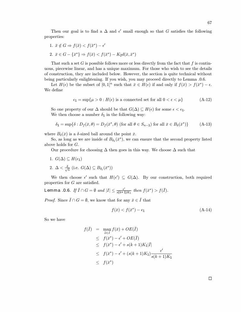
67

Then our goal is to Þnd a ∆ and $$ small enough so that G satisÞes the followingproperties:

1. x /∈ G⇒ f(x) < f(x∗)− $$

2. x ∈ G− {x∗}⇒ f(x) < f(x∗)−K2d(x, x∗)

That such a set G is possible follows more or less directly from the fact that f is contin-uous, piecewise linear, and has a unique maximum. For those who wish to see the detailsof construction, they are included below. However, the section is quite technical withoutbeing particularly enlightening. If you wish, you may proceed directly to Lemma .0.6.

Let H($) be the subset of [0, 1]n such that x ∈ H($) if and only if f(x) > f(x∗) − $.We deÞne

$1 = sup{µ > 0 : H($) is a connected set for all 0 < $ < µ} (A-12)

So one property of our ∆ should be that G(∆) ⊆ H($) for some $ < $1.We then choose a number δ1 in the following way:

δ1 = sup{δ : Df (x, θ) = Df (x∗, θ) (for all θ ∈ Sn−1) for all x ∈ Bδ(x∗)} (A-13)

where Bδ(x) is a δ-sized ball around the point x.So, as long as we are inside of Bδ1(x

∗), we can ensure that the second property listedabove holds for G.

Our procedure for choosing ∆ then goes in this way. We choose ∆ such that

1. G(∆) ⊆ H($1)2. ∆ < δ√

n(i.e. G(∆) ⊆ Bδ1(x

∗))

We then choose $$ such that H($$) ⊆ G(∆). By our construction, both requiredproperties for G are satisÞed.

Lemma .0.6. If I ∩G = ∅ and |I| ≤ +"s(k+1)K1

then f(x∗) > f(I).

Proof. Since I ∩G = ∅, we know that for any x ∈ I that

f(x) < f(x∗)− $1 (A-14)

So we have

f(I) = maxx∈I

f(x) +OE(I)

≤ f(x∗)− $$ +OE(I)≤ f(x∗)− $$ + s(k + 1)K1|I|≤ f(x∗)− $$ + (s(k + 1)K1)

$$

s(k + 1)K1

≤ f(x∗)

68

Lemma .0.7. If I ∩G ,= ∅ and |I| ≤ min{ K2s(k+1)K1

d(x∗, I), +"s(k+1)K1

} then f(x∗) > f(I).

Proof. Since I ∩G ,= ∅, we know that

x ∈ I ⇒ f(x) < f(x∗)−min{K2d(x∗, I), $$}

Letting K3 = s(k + 1)K1 we have:

f(I) = maxx∈I

f(x) +OE(I)

≤ f(x∗)−min{K2d(x∗, I), $$}+OE(I)

≤ f(x∗)−min{K2d(x∗, I), $$} + s(k + 1)K1|I |

≤ f(x∗)−min{K2d(x∗, I), $$}+K3min{K2

K3d(x∗, I),

$$

K3}

≤ f(x∗)

Using this set G, we will now construct a resolution pattern (as a function of R) whichsatisÞes the properties of Lemma .0.1. Then, by counting the size of the resolution patternas a function of R, we can use Proposition .0.2 to calculate the complexity of this class ofproblems with respect to CFDP.

Recall that a resolution pattern P consists of n interval partitions Pj. We will give aprocess to create an interval partition for arbitary j which will yield our resolution patternP . SpeciÞcally, we will create a sequence of interval partitions P 0

j , P1j , P

2j , . . . , P

mj . We

then create one more set, called Qj to ensure the legality of our eventual partition and

then let Pj =9&m

i=1 Pij

:∪Qj . It is useful to keep in mind that we are creating a partition

such that every rectangle I ∈ A(P) will either have f(I) < f(x∗) or |I| = l.With this in mind, our Þrst goal is to ensure that any rectangle I ∈ A(P) such that

I ∩ G = ∅ has the property that |I| ≤ +"s(k+1)K1

. In fact, we would like all I ∈ A(P) tohave this property. This is accomplished quite simply. Choose the smallest integer a suchthat 1

2a <+"

s(k+1)K1. Now we let:

P 0j = {

1

2a,2

2a,3

2a,4

2a, . . . ,

2a

2a} (A-15)

This step alone ensures that when we create our resolution pattern P , that everyI ∈ A(P) has |I| < +"

s(k+1)K1. Therefore, every I such that I ∩ G = ∅ will have the

property that f(I) < f(x∗).Now our goal is to make our resolution pattern reÞned enough so that every I such

that I ∩ G ,= ∅ either has |I | = l (i.e. so I ∈ M(R)) or has the property that |I| <K2

s(k+1)K1d(x∗, I). If the latter property holds, since we are already assured that I | <

+"s(k+1)K1

, we can use Lemma .0.7 to conclude that f(I) < f(x∗).To simplify our notation we will let C1 =

K2s(k+1)K1

. So our goal is to ensure that

|I| ≤ max{C1d(x∗, I), l}. To do this, we construct our interval partitions in such a way so

that if an interval Ij ∈ P $j (the corresponding interval decomposition) and |Ij| = 2yl, then

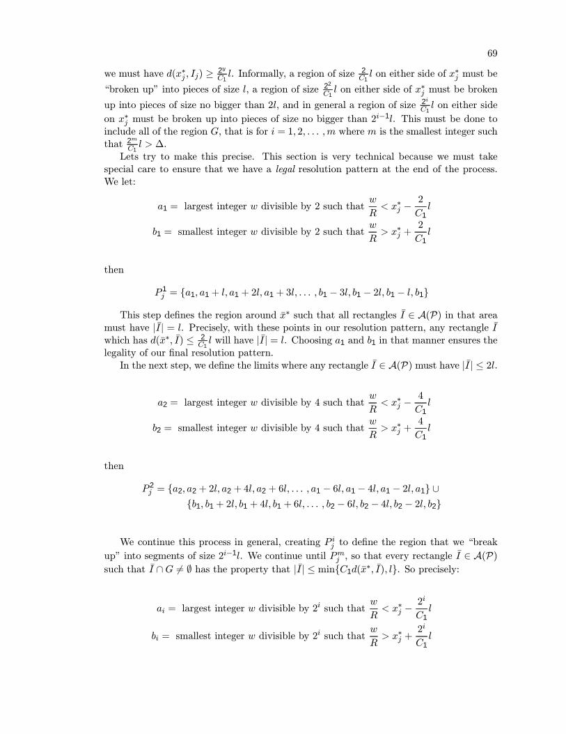
69

we must have d(x∗j , Ij) ≥ 2y

C1l. Informally, a region of size 2

C1l on either side of x∗j must be

�broken up� into pieces of size l, a region of size 22

C1l on either side of x∗j must be broken

up into pieces of size no bigger than 2l, and in general a region of size 2i

C1l on either side

on x∗j must be broken up into pieces of size no bigger than 2i−1l. This must be done to

include all of the region G, that is for i = 1, 2, . . . ,m where m is the smallest integer suchthat 2m

C1l > ∆.

Lets try to make this precise. This section is very technical because we must takespecial care to ensure that we have a legal resolution pattern at the end of the process.We let:

a1 = largest integer w divisible by 2 such thatw

R< x∗j −

2

C1l

b1 = smallest integer w divisible by 2 such thatw

R> x∗j +

2

C1l

then

P 1j = {a1, a1 + l, a1 + 2l, a1 + 3l, . . . , b1 − 3l, b1 − 2l, b1 − l, b1}

This step deÞnes the region around x∗ such that all rectangles I ∈ A(P) in that areamust have |I| = l. Precisely, with these points in our resolution pattern, any rectangle Iwhich has d(x∗, I) ≤ 2

C1l will have |I| = l. Choosing a1 and b1 in that manner ensures the

legality of our Þnal resolution pattern.In the next step, we deÞne the limits where any rectangle I ∈ A(P) must have |I| ≤ 2l.

a2 = largest integer w divisible by 4 such thatw

R< x∗j −

4

C1l

b2 = smallest integer w divisible by 4 such thatw

R> x∗j +

4

C1l

then

P 2j = {a2, a2 + 2l, a2 + 4l, a2 + 6l, . . . , a1 − 6l, a1 − 4l, a1 − 2l, a1} ∪

{b1, b1 + 2l, b1 + 4l, b1 + 6l, . . . , b2 − 6l, b2 − 4l, b2 − 2l, b2}

We continue this process in general, creating P ij to deÞne the region that we �break

up� into segments of size 2i−1l. We continue until Pmj , so that every rectangle I ∈ A(P)such that I ∩G ,= ∅ has the property that |I| ≤ min{C1d(x

∗, I), l}. So precisely:

ai = largest integer w divisible by 2i such thatw

R< x∗j −

2i

C1l

bi = smallest integer w divisible by 2i such thatw

R> x∗j +

2i

C1l

70

then

P ij = {ai, ai + 2i−1l, ai + 2(2i−1)l, ai + 3(2

i−1)l, . . . , ai−1 − 2(2i−1)l, ai−1 − 2i−1l, ai−1} ∪{bi−1, bi−1 + 2

i−1l, bi−1 + 2(2i−1)l, bi−1 + 3(2

i−1)l, . . . , bi − 2(2i−1)l, bi − 2i−1l, bi}

we do this for all i = 1, 2, . . . ,m where again m = 5log2CR∆6. Note that m =O(logR).

By our construction, we have taken care to make sure that our pattern is legal withinG. The only region where our pattern might not be legal is around am and bm. To ensurethe overall legality, we must ensure that all the �ancestors� of these points are in ourinterval partition Pj . So we let:

Qj = { the ancestors of am, bm in the legality tree } (A-16)

Since the depth of the tree is log2(R), clearly |Qj | ≤ 2 log2(R).Finally we let

Pj =

;m%i=0

P ij

<∪Qj (A-17)

and let

P = (P1, P2, . . . , Pn) (A-18)

It is straightforward from our construction that P fulÞlls the criteria of Lemma .0.1and is therefore sufficient. Now we need only verify how |P| grows with R.Lemma .0.8. Under our construction, |P| = O(logR).Proof. We know that |P| ≤$m

i=0 |P ij |. Furthermore, |P 0j | is a constant independent of R,

call it C0. It is also not difficult to see that:

|P 1j | ≤

4C1l

l+ 4 =

4

C1+ 4

which is also independent of R. Moreover, for i = 2, 3, . . . ,m.

|P ij | =2i

C1l

2i−1l+ 4

=2

C1+ 4

So we get:

|P| ≤ C0 +4

C1+ 4 + (m− 1)( 2

C1+ 4) + 2 log2(R)

≤ C2 +mC3 + 2 log2(R) for some constants C2, C3 independent of R

≤ O(logR) since m = O(logR)

71

So we have a sequence of sufficient resolution patterns P(R) such that |P(R)| =O(logR). By Proposition .0.2 we can conclude that our CFDP run time is O((logR)k+2).

Theorem for C2 functions

Theorem .0.9. Suppose the fj are C2 and that f has a unique maximum x∗. Assume

further that the Taylor expansion of f at x∗ has a negative-deÞnite matrix coefficient inthe quadratic term and that f respects a graph of tree-width k. Finally, assume there existssome R1 such that R > R1 implies I

∗ is unique. Then coarse-to-Þne dynamic programmingwill Þnd the rectangle I∗(R) in time O(R

k+22 ).

Proof. The proof for this theorem is nearly identical to the previous proof. Once again,the overestimate factor can be bounded since f is continuous on a compact set. Again,we deÞne a set G which is a neighborhood of x∗ and use it to create a sufficient resolutionpattern P for any big enough resolution R. However, in this case, the relation betweenthe distance of point x ∈ G from x∗ and the difference f(x∗) − f(x) will be quadratic,rather than linear. Thus when we use the properties of G to form |P|, we will Þnd that|P| = O(√R). As a result, our Þnal CFDP complexity will be O((√R)k+2) rather thanO((logR)k+2).

Since f is C2, and [0, 1]n is compact, we can Þnd a constant K1 > 0 such that:

K1 > max{| ∂fi∂xj

(x)|, | ∂f∂xj

(x)|} (A-19)

where the max is taken over all i ∈ 1, 2, . . . s, all j ∈ 1, 2, . . . , n and all x ∈ [0, 1]n wherethe partial derivatives exist.

Lemma .0.10. Recall that we deÞned OE(I) = f(I) − supx∈I f(x). Under the assump-tions of our theorem we have:

OE(I) ≤ s(k + 1)K1|I| (A-20)

Proof. The proof is identical to that of Lemma .0.5 in the previous proof.

We will now create the set G for this problem. SpeciÞcally, we will Þnd a ∆ > 0, $$ > 0and K2 > 0 such that if we deÞne G by:

x ∈ G⇐⇒ xj ∈ [x∗j −∆, x∗j +∆] (A-21)

then we have the following properties

1. x /∈ G⇒ f(x) < f(x∗)− $$

2. x ∈ G⇒ f(x) < f(x∗)−K2d(x, x∗)2

By expanding f in a Taylor Series, and using the fact that x∗ is a maximum, we get:

f(x∗)− f(x∗ + h) = −q(h)−R2(h) (A-22)

72

where q(h) is a negative-deÞnite quadratic and R2(h) = o(|h|2). That is,

lim|h|→0

R2(h)

|h|2 = 0 (A-23)

Note that we can rewrite q(h) as

q(h) = |h|2q+h

|h|,

(A-24)

Now let:

M = min|h|=1

{−q+h

|h|,}

and let K2 =M2 . Since R2(h) = o(|h|2), we can Þnd an h0 such that:

|h| < h0 ⇒ |R2(h)| < K2|h|2

So for |h| < h0 we have:

f(x∗)− f(x) = −q(h)−R2(h)

≥ M |h|2 −K2|h|2≥ K2|h|2

So if G ⊆ Bh0(x∗) then we are assured that the second of our two required properties

is fulÞlled. Now we need only ensure the Þrst property. We can do this by choosing $$ > 0such that:

{x : f(x) ≥ f(x∗)− $$} ⊆ Bh0(x∗)

Since f is continuous and x∗ is a unique maximum we are guaranteed to Þnd such an $$.Now we just choose ∆ < h0

n . By our construction, our set G satisÞes both of the requiredproperties.

Lemma .0.11. If I ∩G = ∅ and |I| ≤ +"skK1

then f(x∗) > f(I).

Proof. The proof is identical to Lemma 3.6.1 in the linear case.

Lemma .0.12. If I∩G ,= ∅ and |I| ≤ min{ K2s(k+1)K1

d(x∗, I)2, +"s(k+1)K1

} then f(x∗) > f(I).

Proof. Since I ∩G ,= ∅, we know that:x ∈ I ⇒ f(x) < f(x∗)−min{K2d(x

∗, I)2, $$}

Letting K3 = s(k + 1)K1, we have:

f(I) = maxx∈I

f(x) +OE(I)

≤ f(x∗)−min{K2d(x∗, I)2, $$}+OE(I)

≤ f(x∗)−min{K2d(x∗, I)2, $$} + s(k + 1)K1|I |

≤ f(x∗)−min{K2d(x∗, I)2, $$}+K3min{K2

K3d(x∗, I)2,

$$

K3}

≤ f(x∗)

73

In a similar way to the previous proof, we construct our resolution pattern P . LetC1 =

K2s(k+1)K1

.

P 0j = {

1

2a,2

2a,3

2a,4

2a, . . . ,

2a

2a} (A-25)

a1 = largest integer w divisible by 2 such thatw

R< x∗j −

?2

C1

√l

b1 = smallest integer w divisible by 2 such thatw

R> x∗j +

?2

C1

√l

then

P 1j = {a1, a1 + l, a1 + 2l, a1 + 3l, . . . , b1 − 3l, b1 − 2l, b1 − l, b1}

a2 = largest integer w divisible by 4 such thatw

R< x∗j −

?4

C1

√l

b2 = smallest integer w divisible by 4 such thatw

R> x∗j +

?4

C1

√l

then

P 2j = {a2, a2 + 2l, a2 + 4l, a2 + 6l, . . . , a1 − 6l, a1 − 4l, a1 − 2l, a1} ∪

{b1, b1 + 2l, b1 + 4l, b1 + 6l, . . . , b2 − 6l, b2 − 4l, b2 − 2l, b2}

ai = largest integer w divisible by 2i such thatw

R< x∗j −

@2i

C1

√l

bi = smallest integer w divisible by 2i such thatw

R> x∗j +

@2i

C1

√l

then

P ij = {ai, ai + 2i−1l, ai + 2(2i−1)l, ai + 3(2

i−1)l, . . . , ai−1 − 2(2i−1)l, ai−1 − 2i−1l, ai−1} ∪{bi−1, bi−1 + 2

i−1l, bi−1 + 2(2i−1)l, bi−1 + 3(2

i−1)l, . . . , bi − 2(2i−1)l, bi − 2i−1l, bi}

we do this for all i = 1, 2, . . . ,m where again m = 5log2CR∆26. Note that m =

O(logR).

74

Finally, we let:

Qj = { the ancestors of am, bm in the legality tree } (A-26)

Since the depth of the tree is log2(R), clearly |Qj | ≤ 2 log2(R).Again we deÞne:

Pj =

;m%i=0

P ij

<∪Qj (A-27)

and let

P = (P1, P2, . . . , Pn) (A-28)

From our construction, we have forced any rectangle I to either have minimum lengthl or to have the property that f(I) < f(x∗). So by Lemma .0.1, we can conclude that Pis sufficient.

Lemma .0.13. Under our construction, |P| = O(√R).Proof. We know that |P| ≤$m

i=0 |P ij |. Furthermore, |P 0j | is a constant independent of R,

call it C0. It is also not difficult to see that:

|P 1j | ≤

2-

2C1

√l

l+ 4 = C2

√R+ 4

which is also independent of R. Moreover, for i = 2, 3, . . . ,m.

|P ij | =2C1(√2i −

√2i−1)

√l

2i−1l+ 4

=2C1(√2− 1)(

√2i−1)

√R

2i−1+ 4

=C3

√R√

2i−1+ 4

Recall that m = 5log2CR∆26 so we can say m ≤ log2 2CR∆

2

So we get:

|P| ≤ C0 +C2

√R+ 4 +

m#i=2

(C3

√R√

2i−1+ 4) + 2 log2(R)

≤ C0 +C2

√R+ 4m+ C3(

√R)

+1√2+

1√4+

1√8+ . . .+

1√2m

,+ 2 log2(R)

≤ C0 +C2

√R+ 4m+ C3(

√R)(1 +

√2) + 2 log2(R)

≤ C0 +C2

√R+ 4(log(2CR∆2) + C3(1 +

√2)√R+ 2 log2(R)

= O(√R)

75

So we have constructed a sequence of legal, sufficient resolution patterns P(R) for R→∞,with the property that |P(R)| = O(√R). By Proposition .0.2 the CFDP complexity forthese problems is O(R

k+22 ).

Bibliography

[1] E. Amir. Efficient approximation for triangulation of minimum tree-width. In Proceed-ings of the Seventeenth Conference on Uncertainty in ArtiÞcial Intelligence. MorganKaufmann, 2001.

[2] S. Arnborg. Efficient algorithms for combinatorial problems on graphs with boundeddecomposability � a survey. BIT, 25:2�23, 1985.

[3] S. Arnborg, D. G. Corneil, and A. Proskurowski. Complexity of Þnding embeddingsin a k-tree. SIAM Journal on Algebraic and Discrete Methods, 8(2):277�284, 1987.

[4] A. Becker and D. Geiger. A sufficiently fast algorithm for Þnding close to optimaljunction trees. In Proceedings of the Twelfth Conference on Uncertainty in ArtiÞcialIntelligence, pages 81�89. Morgan Kaufmann, 1996.

[5] R. Bellman. Dynamic Programming. Princeton University Press, Princeton, N.J.,1957.

[6] U. Bertele and F. Brioschi. Nonserial Dynamic Programming. Academic Press, 1972.

[7] C. Cannings, T. E.A., and H. Skolnick. Probability functions on complex pedigrees.Advances in Applied Probability, 10:26�61, 1978.

[8] P. A. Cohen P., Chaudhri V. and S. R. Does prior knowledge facilitate the develop-ment of knowledge-based systems. In AAAI Proceedings �99, pages 221�226, 1999.

[9] R. Dechter. Bucket elimination: A unifying framework for probabilistic inference. InM. Jordan, editor, Learning in Graphical Models. MIT Press, 1999.

[10] B. Frey. Graphical Models for Machine Learning and Digital Communication. MITPress, 1998.

[11] R. Gallager. Low-Density Parity-Check Codes. PhD thesis, Massachusetts Instituteof Technology, 1963.

[12] S. Geman and K. Kochanek. Dynamic programming and the representation of soft-decodable codes. IEEE Transactions on Information Theory, 47(2):549�568, 2001.

[13] J. Hammersley and P. Clifford. Markov Þelds on Þnite graphs and lattices. Technicalreport, University of California, Berkeley, 1968.

[14] F. V. Jensen and F. Jensen. Optimal junction trees. In R. Mantaras and D. Poole,editors, Proceedings of the Tenth Conference on Uncertainty in ArtiÞcial Intelligence,pages 360�366. Morgan Kaufmann, 1994.

76

77

[15] U. Kjaerulff. Aspects of Efficiency Improvement in Bayesian Networks. PhD thesis,Aalborg University, Department of Mathematics and Computer Science, 1993.

[16] K. Kochanek. Dynamic Programming Algorithms for Maximum Likelihood Decoding.PhD thesis, Division of Applied Mathematics, Brown University, 1998.

[17] S. Lauritzen and D. Speigelhalter. Local computations with probabilities on graphicalstructures and their application to expert systems. Journal of the Royal StatisticalSociety, Series B (Methodological), 50(2):157�224, 1988.

[18] D. B. Lenat. Cyc: A large-scale investment in knowledge infrastructure. Comm.ACM, 38(11):33�38, 1995.

[19] J. Pearl. Probabilistic Reasoning in Intelligent Systems. Morgan Kaufmann, 1988.

[20] M. B. Pradhan M., Provan G. and H. M. Knowledge engineering for large beliefnetworks. In Proceedings of the Tenth Conference on Uncertainty in ArtiÞcial Intel-ligence, pages 484�490, 1994.

[21] S. Ramachandramurthi. The structure and number of obstructions to treewidth.SIAM Journal of Discrete Mathematics, 10(1):146�157, 1997.

[22] C. Raphael. Coarse-to-Þne dynamic programming. IEEE Transactions on PatternAnalysis and Machine Intelligence, 23(12):1379�1390, 2001.

[23] C. Raphael and S. Geman. A grammatical approach to mine detection. In Detec-tion and Remediation Technologies for Mines and Minelike Targets II, Proceedings ofSPIE, pages 316�332, 1997.

[24] B. Ripley. Pattern Recognition and Neural Networks. Cambridge University Press,1996.

[25] N. Robertson and P. D. Seymour. Graph minors ii: algorithmic aspects of treewidth.Journal of Algorithms, 7:309�322, 1986.

[26] N. Robertson and P. D. Seymour. Graph minors xiii: the disjoint paths problem.Journal of Comb. Theory, Series B, 63:65�110, 1995.

[27] D. J. Rose. Triangulated graphs and the elimination process. Journal of MathematicalAnalysis and Applications, 32:597�609, 1970.

[28] D. J. Rose. On simple characterizations of k-trees. Discrete Mathematics, 7:317�322,1974.

[29] R. E. Tarjan and M. Yannakakis. Simple linear-time algorithms to test chordalityof graphs, test acyclicity of hypergraphs, and selectively reduce acyclic hypergraphs.SIAM Journal of Computing, 13(3):566�579, 1984.