Dynamic Probit models for panel data: A comparison … 3 Methods Monte Carlo Study Simulation...

Motivation

3 Methods

Monte CarloStudy

Simulationresults

Conclusions

Dynamic Probit models for panel data: Acomparison of three methods of estimation

Alfonso Miranda

Keele University and IZA([email protected])

2007 UK Stata Users Group meeting

September 10.

Centre for Economic Research · Research Institute for Public Policy and Management

Motivation

3 Methods

Monte CarloStudy

Simulationresults

Conclusions

Motivation

I In a number of contexts researchers have to model adummy variable yit that is function of yi ,t−1

(unemployment, migration, health).

I A dynamic probit/logit model is needed.

I In the dynamic setup yi0 is likely to be correlated withunobserved heterogeneity ui affecting yit .

I If yi0 is taken as exogenous inconsistent estimators areobtained. This is know as the initial conditions problem.


Motivation

3 Methods

Monte CarloStudy

Simulationresults

Conclusions

Motivation

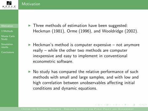
I Three methods of estimation have been suggested:Heckman (1981), Orme (1996), and Wooldridge (2002).

I Heckman’s method is computer expensive – not anymorereally – while the other two methods are computerinexpensive and easy to implement in conventionaleconometric software.

I No study has compared the relative performance of suchmethods with small and large samples, and with low andhigh correlation between unobservables affecting initialconditions and dynamic equations.


Motivation

3 Methods

Monte CarloStudy

Simulationresults

Conclusions

Heckman (1981) method

Heckman suggests to approximate the reduced form of the marginalprobability of yi0 given ui with a Probit model and to allow freecorrelation ρ between yi0 and yit .

y∗it = zitβ + γyi,t−1 + ui + εit (1)

y∗i0 = xitθ + δui + ηit (2)

with yit = 1 if y∗it > 0 and zero otherwise. ui , ηit and εit are all iid

N(0, 1). Neither εit nor ηit are serially correlated.

I equations (1) and (2) are estimated as a system.

I Need to integrate out ui against the density φ(ui ).

I May use ML + Gauss-Hermite quadrature or MaximumSimulated Likelihood.

I ρ = δ√(2(δ2+1))


Motivation

3 Methods

Monte CarloStudy

Simulationresults

Conclusions

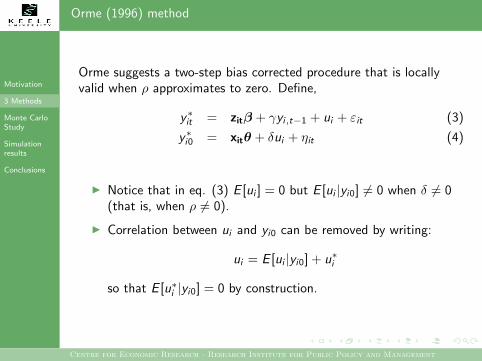
Orme (1996) method

Orme suggests a two-step bias corrected procedure that is locallyvalid when ρ approximates to zero. Define,

y∗it = zitβ + γyi,t−1 + ui + εit (3)

y∗i0 = xitθ + δui + ηit (4)

I Notice that in eq. (3) E [ui ] = 0 but E [ui |yi0] 6= 0 when δ 6= 0(that is, when ρ 6= 0).

I Correlation between ui and yi0 can be removed by writing:

ui = E [ui |yi0] + u∗i

so that E [u∗i |yi0] = 0 by construction.


Motivation

3 Methods

Monte CarloStudy

Simulationresults

Conclusions

Orme (1996) method

I Can use, in a first step, a simple probit model for yi0 toestimate,

E [u|yi0] = E [ui |δui + ηit ≥ −xitθ] =φ (xitθ)

Φ (xitθ)

I And in a second step estimate the dynamic equation using astandard RE probit that includes E [u∗i |yi0] as a regressor,

y∗it = xitβ + γyi,t−1 + σE [ui |yi0] + u∗i + εit (5)

I Orme shows that this two-step procedure is locally valid if ρapproximates to zero and argues that the method can performwell even if ρ is ‘high’.


Motivation

3 Methods

Monte CarloStudy

Simulationresults

Conclusions

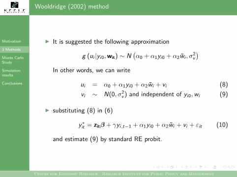
Wooldridge (2002) method

y∗it = xitβ + γyi,t−1 + ui + εit (6)

y∗i0 = zitθ + δui + ηit (7)

I Heckman does the following:

f (yi0, · · · , yiT ) =

Zf (yi1, · · · , yiT |yi0,wit, ui ) h (yi0|wit, ui ) g(ui |wit)dui

with wit = (xit, zit) and use ML.

I Wooldridge suggests to model the distribution of {yi1, · · · , yiT}given yi0 and to use conditional ML.

I To do so one needs to specify the distribution for ui given yi0

and other exog. variables:

f (yi1, · · · , yiT |yi0) =

Zf (yi1, · · · , yiT |yi0,wit, ui ) g (ui |yi0,wit) dui


Motivation

3 Methods

Monte CarloStudy

Simulationresults

Conclusions

Wooldridge (2002) method

I It is suggested the following approximation

g (ui |yi0,wit) ∼ N(α0 + α1yi0 + α2w̄i , σ

2v

)In other words, we can write

ui = α0 + α1yi0 + α2w̄i + vi (8)

vi ∼ N(0, σ2v ) and independent of yi0,wi (9)

I substituting (8) in (6)

y∗it = zitβ + γyi,t−1 + α1yi0 + α2w̄i + vi + εit (10)

and estimate (9) by standard RE probit.


Motivation

3 Methods

Monte CarloStudy

Simulationresults

Conclusions

Monte Carlo Study

The following model is specified:

y∗it = 0.5 + 0.5zit − 0.5yi,t−1 + ui + εit (11)

y∗i0 = 1xi0 − 1zi0 + δui + ηit (12)

I Random draws from independent standard normal distributionsare taken to generate zit and xi0. These variables remain fixedduring all simulations.

I At each replication step random draws from independentstandard normal distributions are taken to generate ui , εit andηit .

I At each iteration the model is estimated using Heckman (MSLwith 400 halton draws), Wooldridge, and Orme methods.Estimates for the dynamic equation are kept.


Motivation

3 Methods

Monte CarloStudy

Simulationresults

Conclusions

Monte Carlo Study

I 1000 replications are taken.

I Various experiments are done comparing the performance of allthese three methods using small, medium, and large samplesand low and high ρ.

I At the end simulation statistics are calculated:

I Average estimator (AE)I Percentage bias (PB)I Average standard error (ASE)I Standard error (SDE)I Mean square error (MSE)I Nominal coverage of 95% confidence intervals (Ncov).


Motivation

3 Methods

Monte CarloStudy

Simulationresults

Conclusions

T=3, n=100, N=300, rho=0

Number of panels = 100Obs per panel = 3Total Number of obs = 300Delta = 0.00------------------------------------------------

| AE | PB | ASE | SDE | MSE | Ncov------------------------------------------------Heckman Method

z .506 1.21 .14 .136 .019 .958LDV -.506 -1.14 .261 .25 .063 .958

_cons .51 1.93 .221 .22 .048 .948Wooldridge Method

z .5 .015 .168 .171 .029 .956LDV -.452 9.59 .36 .369 .138 .93

_cons .494 1.13 .332 .352 .124 .926Orme Method

z .502 .461 .148 .151 .023 .952LDV -.48 4.08 .352 .355 .127 .931

_cons .488 -2.36 .326 .333 .111 .93------------------------------------------------


Motivation

3 Methods

Monte CarloStudy

Simulationresults

Conclusions

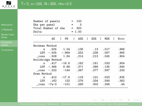
T=3, n=100, N=300, rho=0.5

Number of panels = 100Obs per panel = 3Total Number of obs = 300Delta = 1.00--------------------------------------------------------

AE | PB | ASE | SDE | MSE | Ncov--------------------------------------------------------Heckman Method

z .505 1.04 .136 .13 .017 .966LDV -.505 -.969 .252 .238 .057 .965


z .417 -16.6 .162 .161 .033 .904LDV -.466 6.88 .371 .366 .135 .945

_cons -.222 -144 .267 .277 .597 .232Orme Method

z .412 -17.6 .118 .121 .023 .835LDV .162 132 .276 .334 .549 .362

_cons -7e-3 -101 .266 .302 .348 .44----------------------------------------------------------


Motivation

3 Methods

Monte CarloStudy

Simulationresults

Conclusions

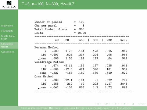
T=3, n=100, N=300, rho=0.7

Number of panels = 100Obs per panel = 3Total Number of obs = 300Delta = 10.00-------------------------------------------------------

AE | PB | ASE | SDE | MSE | Ncov-------------------------------------------------------Heckman Method

z .509 1.78 .131 .123 .015 .962LDV -.497 .525 .237 .224 .05 .968


z .474 -5.16 .159 .157 .025 .943LDV -.564 -12.8 .421 .396 .161 .932

_cons -.327 -165 .182 .189 .719 .022Orme Method

z .389 -22.1 .101 .1 .022 .799LDV .558 212 .19 .223 1.17 3e-3

_cons -.042 -108 .853 1.2 1.72 .849---------------------------------------------------------


Motivation

3 Methods

Monte CarloStudy

Simulationresults

Conclusions

T=3, n=300, N=900, rho=0

Number of panels = 300Obs per panel = 3Total Number of obs = 900Delta = 0.00-------------------------------------------------------

| AE | PB | ASE | SDE | MSE | Ncov-------------------------------------------------------Heckman Method

z .505 .941 .077 .078 6e-03 .948LDV -.492 1.54 .147 .142 .02 .962

_cons .497 -.587 .126 .12 .014 .961Wooldridge Method

z .488 -2.49 .09 .088 8e-3 .947LDV -.399 20.3 .197 .205 .052 .904

_cons .46 -7.9 .185 .193 .039 .928Orme Method

z .491 -1.83 .081 .082 7e-3 .931LDV -.436 12.8 .195 .198 .043 .922

_cons .452 -9.67 .179 .18 .035 .928-------------------------------------------------------


Motivation

3 Methods

Monte CarloStudy

Simulationresults

Conclusions

T=3, n=300, N=900, rho=0.5



z .504 .88 .075 .076 6e-3 .948LDV -.493 1.34 .142 .135 .018 .964


z .421 -15.9 .088 .089 .014 .823LDV -.442 11.6 .21 .231 .057 .938

_cons -.225 -145 .153 .153 .549 7e-3Orme Method

z .401 -19.9 .068 .07 .015 .62LDV .209 142 .167 .207 .545 .112

_cons -.048 -110 .155 .177 .332 .174---------------------------------------------------------


Motivation

3 Methods

Monte CarloStudy

Simulationresults

Conclusions

T=3, n=300, N=900, rho=0.7

Number of panels = 300Obs per panel = 3Total Number of obs = 900Delta = 10.00----------------------------------------------------------

AE | PB | ASE | SDE | MSE | Ncov----------------------------------------------------------Heckman Method

z .506 1.22 .071 .07 5e-3 .957LDV -.49 2 .133 .127 .016 .955


z .472 -5.58 .088 .086 8e-3 .928LDV -.517 -3.46 .267 .245 .06 .924

_cons -.33 -166 .103 .1 .699 0Orme Method

z .399 -20.1 .058 .06 .014 .567LDV .575 215 .109 .126 1.17 0

_cons -.27 -154 .555 .796 1.23 .58----------------------------------------------------------


Motivation

3 Methods

Monte CarloStudy

Simulationresults

Conclusions

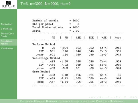
T=3, n=3000, N=9000, rho=0



z .5 -.024 .023 .022 5e-4 .962LDV -.501 -.176 .046 .046 2e-3 .951

_cons .501 .134 .039 .039 1e-3 .948Wooldridge Method

z .493 -1.38 .028 .026 7e-4 .959LDV -.464 7.23 .069 .063 5e-3 .939

_cons .483 -3.3 .061 .06 4e-3 .944Orme Method

z .493 -1.48 .025 .024 6e-4 .95LDV -.469 6.12 .065 .059 4e-3 .944

_cons .477 -4.64 .06 .055 3e-3 .946---------------------------------------------------------


Motivation

3 Methods

Monte CarloStudy

Simulationresults

Conclusions

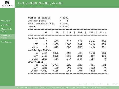
T=3, n=3000, N=9000, rho=0.5

Number of panels = 3000Obs per panel = 3Total Number of obs = 9000Delta = 1.00---------------------------------------------------------

AE | PB | ASE | SDE | MSE | Ncov---------------------------------------------------------Heckman Method

z .5 .059 .023 .021 4e-4 .968LDV -.5 -.063 .045 .044 2e-3 .955

_cons .5 .049 .038 .038 1e-3 .951Wooldridge Method

z .419 -16.3 .026 .03 7e-3 .163LDV -.415 16.9 .062 .101 .017 .486

_cons -.218 -144 .047 .047 .517 0Orme Method

z .397 -20.7 .022 .025 .011 .02LDV .245 149 .06 .085 .562 0

_cons -.081 -116 .054 .07 .342 0---------------------------------------------------------


Motivation

3 Methods

Monte CarloStudy

Simulationresults

Conclusions

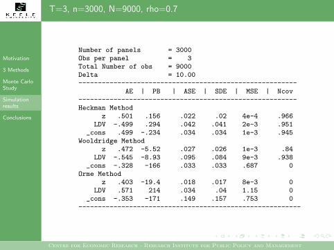
T=3, n=3000, N=9000, rho=0.7



z .501 .156 .022 .02 4e-4 .966LDV -.499 .294 .042 .041 2e-3 .951

_cons .499 -.234 .034 .034 1e-3 .945Wooldridge Method

z .472 -5.52 .027 .026 1e-3 .84LDV -.545 -8.93 .095 .084 9e-3 .938

_cons -.328 -166 .033 .033 .687 0Orme Method

z .403 -19.4 .018 .017 8e-3 0LDV .571 214 .034 .04 1.15 0

_cons -.353 -171 .149 .157 .753 0---------------------------------------------------------


Motivation

3 Methods

Monte CarloStudy

Simulationresults

Conclusions

Conclusions

I Heckman’s method delivers estimators that are hardlysubject to bias and that are estimated with high precision.

I The methods suggested by Wooldridge and Orme (W&O)deliver estimators that can be subject to substantial biasand low precision.

I W&O: The bias does not seem to decrease as sample size(number of panels n) increases.

I W&O: The bias increases when ρ gets higher.

I Nominal coverage of confidence intervals is satisfactory inHeckman’s method but can be extremely bad in the caseof W&O when ρ is high.


Motivation

3 Methods

Monte CarloStudy

Simulationresults

Conclusions

Conclusions

I Evidence suggest that Heckman’s method offerssubstantial advantages.

I Today Heckman’s method is not really computer expensiveanymore (can use MSL and BHHH algorithm to speed theprocess).


Dynamic Probit models for panel data: A comparison … 3 Methods Monte Carlo Study Simulation...

Documents

Transcript of Dynamic Probit models for panel data: A comparison … 3 Methods Monte Carlo Study Simulation...