Dynamic pricing under demand uncertainty in the presence ...
106
Dynamic pricing under demand uncertainty in the presence of strategic consumers by Yinhan Meng A thesis presented to the University of Waterloo in fulfillment of the thesis requirement for the degree of Master of Applied Science in Management Sciences Waterloo, Ontario, Canada, 2011 c Yinhan Meng 2011
Transcript of Dynamic pricing under demand uncertainty in the presence ...

Dynamic pricing under demanduncertainty in the presence of
strategic consumers
by
Yinhan Meng
A thesispresented to the University of Waterloo
in fulfillment of thethesis requirement for the degree of
Master of Applied Sciencein
Management Sciences
Waterloo, Ontario, Canada, 2011
c© Yinhan Meng 2011

I hereby declare that I am the sole author of this thesis. This is a true copy of the thesis,
including any required final revisions, as accepted by my examiners.
I understand that my thesis may be made electronically available to the public.
ii

Abstract
We study the effect of strategic consumer behavior on pricing, inventory decisions, and
inventory release policies of a monopoly retailer selling a single product over two periods
facing uncertain demand. We consider the following three-stage two-period dynamic pricing
game. In the first stage the retailer sets his inventory level and inventory release policy;
in the second stage the retailer faces uncertain demand that consists of both myopic and
strategic consumers. The former type of consumers purchase the good if their valuations
exceed the posted price, while the latter type of consumers consider future realizations
of prices, and hence their future surplus, before deciding when to purchase the good; in
the third stage, the retailer releases its remaining inventory according to the release policy
chosen in the first stage.
Game theory is employed to model strategic decisions in this setting. Each of the
strategies available to the players in this setting (the consumers and the retailer) are
solved backward to yield the subgame perfect Nash equilibrium, which allows us to derive
the equilibrium pricing policies.
This work provides three primary contributions to the fields of dynamic pricing and
revenue management. First, if, in the third stage, inventory is released to clear the market,
then the presence of strategic consumers may be beneficial for the retailer. Second, we find
the optimal inventory release strategy when retailers have capacity limitation. Lastly, we
numerically demonstrate the retailer’s optimal decisions of both inventory level and the
inventory release strategy. We find that market clearance mechanism and intermediate
supply strategy may emerge as the retailers optimal choice.
iii

Acknowledgements
It has been my good fortune to have the advice and guidance of many talented people,
whose knowledge and skills have enhanced this thesis in many ways. I would like to thank
my supervisor, Dr. Benny Mantin, for his insightful guidance in advising me with this
thesis. Without his support and encouragement, my contribution to this thesis would not
have been possible. Secondly, I would like to thank Dr. Stanko Dimitrov and Dr. Qi-Ming
He for their careful reviewing and constructive criticism of this thesis.
iv

Dedication
I would like to thank my loving family and my friends. This work would not have been
possible without their continuous support, both financially and emotionally. They have
been tremendously caring and understanding throughout all these years. It was a long
haul, but it is finally done.
v

Table of Contents
List of Figures ix
1 Introduction 1
1.1 Background . . . . . . . . . . . . . . . . . . . . . . . . . . . . . . . . . . . 1
1.2 Problem of Interest . . . . . . . . . . . . . . . . . . . . . . . . . . . . . . . 3
1.3 Overview of Results and Organization of the Thesis . . . . . . . . . . . . . 5
2 Literature Review 8
3 Model Setup 14
4 Preliminary Analysis 20
4.1 Consumer’s Purchasing Behavior . . . . . . . . . . . . . . . . . . . . . . . 20
4.2 Pricing Policies . . . . . . . . . . . . . . . . . . . . . . . . . . . . . . . . . 25
vi

5 Clearance Sales Strategy 28
5.1 Case a: Inventory Depleted Completely over Two-period Sales . . . . . . . 29
5.1.1 Equilibrium Pricing Policies and Model Analysis . . . . . . . . . . . 30
5.1.2 Basic Skim Both and Skim Myopic . . . . . . . . . . . . . . . . . . 34
5.2 Case b: Inventory Depleted Completely in period 1 under High Demand . 48
5.2.1 The Switching Sequence When δ ≤ δa . . . . . . . . . . . . . . . . . 52
5.2.2 The Switching Sequence When δ > δa . . . . . . . . . . . . . . . . . 57
5.3 Case c: Possible Leftover Inventory after Clearance Sales . . . . . . . . . . 61
5.4 Summary of Clearance Sale Strategy . . . . . . . . . . . . . . . . . . . . . 67
6 Optimal Release Strategy 72
6.1 Dynamic Pricing Strategy . . . . . . . . . . . . . . . . . . . . . . . . . . . 72
6.2 Intermediate Supply Strategy . . . . . . . . . . . . . . . . . . . . . . . . . 76
6.2.1 Optimal capacity is employed for Skim Both under Intermediate Sup-
ply Strategy . . . . . . . . . . . . . . . . . . . . . . . . . . . . . . . 79
6.2.2 Skim Myopic under Intermediate Supply Strategy . . . . . . . . . . 80
6.3 Integrating Clearance Sales, Intermediate Supply and Dynamic Pricing strate-
gies . . . . . . . . . . . . . . . . . . . . . . . . . . . . . . . . . . . . . . . . 83
7 Summary and Managerial Insights 89
vii

Appendices 92
Bibliography 94
viii

List of Figures
3.1 Timeline of the three-stage two-period dynamic pricing game. . . . . . . . 16
4.1 An Example of the relationship among threshold functions and selling price
in period 2 under high demand. . . . . . . . . . . . . . . . . . . . . . . . . 24
4.2 An Example of a Purchasing Strategy of Strategic Consumer Under the
Clearance Sale Senario. . . . . . . . . . . . . . . . . . . . . . . . . . . . . . 27
5.1 The value of δ1. When δ > δ1, the basic CS is employed by the retailer;
when δ < δ1, the retailer employs AH. . . . . . . . . . . . . . . . . . . . . . 32
5.2 The case separation based on α and δ when supply equals demand, where
SB=Skim Both; SM=Skim Myopic and AH=sell All under High demand in
period1. . . . . . . . . . . . . . . . . . . . . . . . . . . . . . . . . . . . . . 34
5.3 Examples of prices and threshold valuations under Clearance Sales strategy,
and basic Skim Both and Skim Myopic cases are employed. . . . . . . . . . 41
5.4 Two examples of profits and corresponding inventory level under Basic Skim
Both and Skim Myopic cases. . . . . . . . . . . . . . . . . . . . . . . . . . 43
ix

5.5 Optimal pricing policy and inventory level under Clearance Sale assuming
AH is employed; δ = 0.35, c = 0.2. . . . . . . . . . . . . . . . . . . . . . . . 55
5.6 Optimal pricing policy and inventory level under Clearance Sale assuming
AH is employed; δ = 0.7, c = 0.2. . . . . . . . . . . . . . . . . . . . . . . . 59
5.7 Optimal pricing policy and inventory level under Clearance Sale assuming
SD is employed; δ = 0.6, c = 0.2. . . . . . . . . . . . . . . . . . . . . . . . 65
5.8 An example of combination of Clearance Sale strategy in the case of δ =
0.35, c = 0.2. . . . . . . . . . . . . . . . . . . . . . . . . . . . . . . . . . . . 68
5.9 An example of combination of Clearance Sale strategy in the case of δ =
0.7, c = 0.2. . . . . . . . . . . . . . . . . . . . . . . . . . . . . . . . . . . . 69
6.1 Two examples of profits and correponding prices and threshold valuations
under Optimal Release strategy. . . . . . . . . . . . . . . . . . . . . . . . . 77
6.2 Retailer’s profit after adoption of an Intermediate Supply strategy; c =
0.1, α = 0.3. . . . . . . . . . . . . . . . . . . . . . . . . . . . . . . . . . . 83
6.3 Profit functions of three inventory release strategies with undecided inven-
tory decision (K) in the case of c = 0.2, α = 0.5 and δ = 0.7. . . . . . . . . 85
6.4 Profit functions of two inventory release strategies with undecided inventory
decision (K) in the case of c = 0.3, α = 0.5 and δ = 0.7. . . . . . . . . . . . 86
6.5 Nine examples are given using different valuations, inventory costs and pa-
tience levels to display the profit functions by using the three inventory
release strategies. . . . . . . . . . . . . . . . . . . . . . . . . . . . . . . . . 88
x

Chapter 1
Introduction
1.1 Background
In recent years, there has been an increasing interest in research on dynamic pricing and
revenue management. Numerous papers have studied revenue management, or markdown
pricing; e.g., Lazear (1986), Gallego and Van Ryzin (1994), Feng and Gallego (1995). The
structure of a markdown mechanism influences buyer behavior, and in turn, the seller’s
profits. Lazear (1986) employs a two step markdown mechanism. The latter two study
demand in a Poisson process with known intensity where they show that prices are not
necessarily decreasing.
The mainstream literature on dynamic pricing has focused, thus far, on managing
clearance prices: finding the optimal timing and magnitude of the discount price along the
selling horizon (see, e.g., Lazear 1986, Feng and Gallego 2000, Aviv and Pazgal 2008, Zhang
1

and Cooper 2008). As research has been maturing in the field of dynamic pricing (DP)
and revenue management (RM) employing passive demand, researchers have shifted their
focus on to modeling strategic consumer behavior. The general result is that the presence
of these consumers is detrimental to firms (Besanko and Winston 1990, Aviv and Pazgal
2008). Besanko and Winston (1990) demonstrate that the retailer’s profit decreases as a
result of mistakenly treating forward-looking consumers as myopic. It has been suggested
that strategic consumer behavior suppresses the benefits of segmentation under medium
to high values of heterogeneity and modest rates of decline in valuations. Also the seller
cannot effectively avoid the adverse impact of strategic behavior even under low levels of
initial inventory (Aviv and Pazgal 2008).
Recently, some researchers have tried to show how to mitigate strategic consumers’
behavior (Liu and van Ryzin 2008, Cachon and Swinney 2009, Levin et al. 2009, Aviv,
Levin and Nediak 2010). Liu and van Ryzin (2008) demonstrate that rationing can be a
profitable strategy to influence the strategic consumers’ behavior. Cachon and Swinney
(2007) study the additional value of quick response to mitigate the negative consequences
of strategic purchase behavior of customers. Levin et al. (2009) demonstrate that the
initial capacity can be used together with the appropriate pricing policy to effectively
reduce the impact of strategic consumer behavior, when the initial capacity is a decision
variable. Aviv, Levin and Nediak (2010) study whether price matching of either internal or
external type can lead to a decrease in strategic waiting by the consumers. Our approach
is to consider a clearance sales mechanism, similar to the market clearance mechanism
employed in Lee and Whang (2002), Cachon and Kok (2007), but with pricing decisions
instead of studying the news vendor model. Lee and Whang (2002) investigate the impacts
2

of a secondary market where retailers can buy and sell excess inventories. Cachon and Kok
(2007) use the clearance sales mechanism to determine the salvage value in the newsvendor
setting.
1.2 Problem of Interest
We study the effect of strategic consumer behavior on pricing, inventory decisions and
inventory release policies of a monopoly retailer selling a single product over two periods
under uncertain demand. Under this premise, the retailer offers opportunity to consumers
that price in period 2 could be lower than the posted price in period 1; while, at the same
time, consumers face the risk that the price may increase in period 2. We are interested in
the benefits that such a mechanism can offer the firm, which can be a better segmentation
of consumers to price discriminatively and/or a significant mitigation of the uncertain
demand to capture more profit. Moreover, we seek to find whether the clearance sales
strategy is always the optimal choice in the context of other inventory release strategies.
Our primary goal in this paper is to address the optimal inventory release strategy when
capacity is know and, ultimately, when the retailer can set the optimal inventory at the
beginning of the selling horizon under uncertain demand.
In our two period selling horizon setting, we assume that a monopoly retailer satisfies
first period demand1 but considers the following two inventory release policies for the second
1This is not a binding constraint under most circumstances, and we find it to be binding in a limitedinterval where the entire inventory is depleted in period 1. Therefore, the results are consistent with theassumption. Liu and van Ryzin (2008) adopted a similar assumption that demand in the first period issatisfied.
3

period: Clearance Sale strategy (CS): all leftover inventory is released to the market and
the market determines the price; Dynamic Pricing strategy (DP): the leftover inventory is
released to maximize the second period profit by ignoring the inventory constraints. We
study the Clearance Sales and Dynamic Pricing strategies separately. The latter policy
gives rise to another instance, which we refer to as Intermediate Supply (IS), which occurs
if the inventory level is at some intermediate level. Specifically, under Intermediate Supply
strategy, if demand is low, the leftover inventory is released to maximize the profit and if
demand is high, the entire leftover inventory is released.
In the model, a fraction of consumers are strategic and time their purchases to maximize
their own expected surplus. Consumers may respond strategically to a retailer’s pricing
decisions, while a myopic consumer acts impulsively and purchases the good if his imme-
diate surplus is positive. Therefore, there is a need to incorporate consumer responses
in the decision-making process. Similar to Cachon and Swinney (2009), we assume that
while myopic consumers visit the store in the first period only, strategic consumers may
return in the second period, and that these strategic consumers possess a discounting factor
associated with their patience level (Levin et al. 2009) or with their reduced discounted
surplus obtained due to the delayed purchase. The number of consumers that arrive in the
first period could be either high or low. Though this information is common knowledge,
the strategic consumers, when they arrive at the store in the first period, do not know the
realization of demand until the end of the first period.
Our work addresses the following research questions: (i) Given an inventory level,
which inventory release policy should the retailer choose under uncertain demand? (ii)
If the retailer can set both the inventory level and the inventory release policy, which
4

inventory release policy should the retailer choose under uncertain demand? (iii) Is the
retailer always better off with lower strategic consumers’ patience levels? (iv) Is the retailer
always better off if fewer strategic consumers exist in the market?
1.3 Overview of Results and Organization of the The-
sis
By employing Clearance Sale strategy, the price that the retailer charges in the second
period may be higher, or lower, than the price posted in the first period. Specifically, if
the demand in the first period is high, more of the inventory is depleted and with lower
remaining inventory, the second period price could be higher than the first period price.
Strategic consumers, when they decide on their purchase timing, should account for the
possibility of the second period price being higher, as this price could very well exceed
their valuations (and they may end up not purchasing at all).
Each of the policies is solved backward to yield the subgame perfect Nash equilibrium,
which allows us to derive the equilibrium pricing policies. We find that for certain param-
eters’ range, the retailer may price to skim high-valuation consumers of both consumer
types (myopic and strategic) in the first period; otherwise, the retailer will price to skim
only high-valuation myopic consumers in the first period, while deferring all strategic con-
sumers to the second period. Quite trivially, in the Dynamic Pricing strategy, we also find
that the prices charged in period 2 are less than the selling price in period 1 under a certain
parameter range.
5

The results of this study indicate that, given the inventory level, a retailer’s profit
function is strictly concave in the inventory quantity stocked under feasible region for both
Clearance Sales (CS) strategy and Intermediate Supply (IS) strategy, which guarantees an
optimal stocking decision under both Clearance Sales and Intermediate Supply strategies.
Thus, the retailer’s profit function is piecewised concave in Clearance Sales and Interme-
diate Supply strategies, and linear in Dynamic Pricing strategy. When the retailer can set
both the inventory level and inventory release policy, it appears that the retailer sets a
rather low inventory level. By employing a low inventory level, the retailer can charge high
prices in the first period, and still retain strategic consumer demand in the second period.
Consistent with some previous studies, we also find that more myopic consumers ex-
isting in the market is beneficial for the retailer, but only when the number is above a
certain threshold. We find that optimal stocking and corresponding profit may decrease
as the proportion of myopic consumers increases under both Clearance Sales and Dynamic
Pricing strategies. Indeed, with fewer strategic consumers, the retailer’s potential profit
from the second period diminishes (recall that only strategic consumers may delay their
purchase to the second period). The retailer cares less about the strategic consumers and
seeks to defer them all to the second period, while focusing attention on first period de-
mand stemming from myopic consumers. Yet, the retailer stocks a lower inventory level
and sets a higher first period price (partially to divert strategic consumers to the second
period). Ultimately, this results in less profit for the retailer. Also, we further prove that,
most of the time, the retailer is better off with less patient strategic consumers under a
simplifying condition (high demand and low demand occur with equal probabilities, and
the magnitude of low demand is half of that of high demand).
6

In the Dynamic Pricing strategy, the analysis reveals that the choice of inventory level
determines the corresponding inventory release in the second period. If the inventory level
is high, leftover inventory is released optimally in the second period; if the inventory level
is intermediate, then Intermediate Supply strategy follows, and eventually, if inventory is
low, Clearance Sales emerges. The choice of stocking level depends on the optimal profit
in each of these outcomes. This strong relationship between the inventory release strategy
and inventory level is demonstrated, which solves our first research question.
Lastly, we compare the profit functions under the different inventory release strategies
in order to characterize the conditions under which each policy is preferred by the retailer
when he can also determine the stocking level. Since it is very difficult to compare an-
alytically the profit functions under the three inventory release strategies, we resort to
numerical examples. Our numerical analysis suggests that the retailer is always better off
with Intermediate Supply strategy than with Dynamic Pricing strategy, and the retailer
is mostly better off employing an Intermediate Supply strategy if he can make decisions
about both inventory level and an inventory release strategy. A few examples also show
that the possibilities of a Clearance Sales strategy dominate sometimes when inventory
costs and/or consumers’ patience levels are high.
The remainder of the paper is organized as follows. Section 2 lays out the theoretical
dimensions of the research and looks at the related literature. The modeling framework and
assumptions are set up in Section 3 and the preliminary analysis is conducted in Section 4.
Section 5 studies the Clearance Sale strategy. Section 6 analyzes Dynamic Pricing and
Intermediate Supply strategies and integrates the different policies to reveal the Optimal
Release strategy. Section 7 summarizes.
7

Chapter 2
Literature Review
A considerable amount of work has been conducted in the area of profit management and
dynamic pricing (e.g., reviews by Bitran and Caldentey 2003, Elmaghraby and Keskinocak
2003, Talluri and van Ryzin 2004, Chan et al. 2004, and Shen and Su 2007). For example,
in their book, Talluri and van Ryzin (2004) provide an extensive review of revenue man-
agement with seat inventory and capacity-planning problems. However, this review focuses
almost exclusively on myopic consumers, and strategic consumers are considered only if
the firm is not capacity constrained. They state that “some industries use price-based RM
(retailing), whereas others use quantity-based RM (airlines).
Even in the same industry, firms may use a mixture of price- and quantity-based RM.
For instance, many of the RM practices of the new low-cost airlines more closely resemble
dynamic pricing than the quantity-based RM of the traditional carriers” (p. 176); Shen
and Su (2007) review previous models of customer behavior in the revenue management
8

and auction literature; Elmaghraby and Keskinocak (2003) focus on dynamic pricing in
the presence of inventory considerations, where they pointed out that the increased avail-
ability of demand data, the ease of changing prices as a result of new technologies and the
availability of decision-support tools for analyzing demand data are the three factors which
contributed to this phenomenon. In our work, a mixture of price- and quantity-based Profit
Management is studied uner demand uncertainty.
At the passive demand research has been maturing in the field of dynamic pricing
(DP) and revenue management (RM), researchers shift their focus to modeling strategic
consumer behavior. And two types of behaviors are analyzed together, which are myopic
and strategic behaviors. The general result is that the presence of this type of consumers
is detrimental to firms (Besanko and Winston 1990, Aviv and Pazgal 2008). Modeling
strategic consumers’ behavior can be traced back to Coase (1972). Gallego and van Ryzin
(1994) characterized the optimal pricing policy in the presence of strategic consumers.
Elmaghraby et al. (2002) analyze the optimal design of a markdown pricing mechanism
in the presence of strategic consumers. Zhou, Fan and Cho (2009) focus on the optimal
purchasing strategy of a single strategic consumer, and they numerically find that strategic
behavior may benefit the retailer. Aviv and Pazgal (2008) study the optimal pricing of a
finite quantity of a fashion-like seasonal good in the presence of forward-looking (strate-
gic) customers. They consider two classes of pricing strategies in their paper: contingent
and announced fixed-discount. We demonstrated that the behavior may actually benefit
retailers.
Some contributes have tried to show how to mitigate such behavior (Liu and van Ryzin
2008, Levin et al. 2009, Aviv, Levin and Nediak 2010). Our approach is to consider the
9

clearance sales mechanism, similar to the market clearance mechanisms demonstrated in
Lee and Whang (2002) and Cachon and Kok (2007). In their works, the clearance mecha-
nism was used to determine the salvage value in the newsvendor model, but the researchers
make no price decisions. Lee and Whang (2002) consider two interdependent effects which
are a quantity effect (sales by the manufacturer) and an allocation effect. Cachon and Kok
(2007) highlight the importance of understanding how a model can interact with its own
inputs.
Continuous updating of prices over time is not a practical pricing policy in the view of
Gallego and van Ryzin (1994) and Bitran and Mondschein (1997). While periodic pricing
policies are employed by Lazear (1986) and Elmaghraby et al. (2002) where prices are
updated at fixed time intervals, Gallego and van Ryzin (1994) set the price to the “optimal”
fixed price to maximize the retailer’s profit. In addition, clearance pricing has been studied
extensively in the operations literature. Here we do not attempt to provide a complete
review. Bitran and Caldentey (2003) and Elmaghraby and Keskinocak (2003) provide
surveys in this field. Zhang and Copper (2008) study the effect of strategic consumer
behavior on pricing and rationing decisions of a firm selling a single product over two
periods. We model a retailer charge a single price in each period, with two price options
in period 2 depending on the demand level.
Numerous studies have attempted to explain the markdown mechanism (e.g., Lazear
1986, Smith and Achabal 1998, Gupta et al. 2006, Zhang and Cooper 2008). Even though
they all refer to the inventory release policy as a clearance sale, their approach is not
a market clearance mechanism as employed in this work. Lazear (1986) and Smith and
Achabal (1998) try to move merchandizes at a price significantly lower than its original
10

price in their studies. In the studies of Gupta et al. (2006) and Zhang and Cooper’ s study
(2008), the seller may limit the availability of the product in the clearance period. In our
model, the retailer may only charge a lower price in latter period of the selling period if
the demand level is low.
This paper shows more about that prices may in fact increase, due, e.g., to limited
supply, and the choice of inventory release policy of retailers. Elmaghraby and Keskinocak
(2003) have also considered whether prices are allowed to increase over time depending
on the underlying modeling assumptions: “current research suggests that prices either
decrease over time (Lazear 1986) or prices move both up and down (Bitran and Mondschein
1997, Feng and Gallego 1995, Gallego and van Ryzin 1994).” Possible explanations for the
rise in price are the stochastic arrival of consumers or the poisson arrivals of consumers
under continuous time and the fact that high valuation consumers arrive later during the
selling season. Although some research has been carried out on this topic, no single study
exists which adequately covers the possibility that limited supply might be one of the
reasons for price rises over time.
Several attempts have been made to study the pricing decisions using different consumer
arrival processes. A deterministic model is studied by Elmaghraby et al. (2002) where
all consumers arrive at the market at the beginning of the selling season with known
valuations. Lazear (1986) uses a simplified model of the stochastic demand. Gallego and
van Ryzin (1994) formulate the problem using intensity control (Bremaud 1980) and
study the optimal dynamic pricing strategy using different demand functions, including
exponential arrival of families, general linear function and compound poisson function.
Feng and Gallego (1995) and Aviv and Pazgal (2008) model the demand as a homogenous
11

(time-invariant) poisson process. Su (2007) model the demand function as the continuous
deterministic arrival of consumers.
Demand is one of the most important elements that influences pricing decisions, a fact
that also explains reactions to price changes and other factors. The variety of products in
the market has significantly risen, while the product life cycles have become shorter in the
last decades. It is even complicated for the retailer to make inventory decisions in advance
if demand is uncertain. Most studies in the field of dynamic pricing have focussed only on
considering initial inventory decisions as exogenously determined. The following literature
consider initial inventory decision as an object decision the retailer must make. Cachon
and Swinney (2009) study the pricing and stocking decisions by a monopolist facing myopic
consumers, bargain-hunters, and strategic consumers. Liu and van Ryzin (2008) focus on
capacity rationing to induce early purchases. Smith and Achabal (1998) and Mantrala
and Rao (2001) study initial inventory decisions as well as markdown pricing decisions
before the selling season in the absence of strategic consumers. We consider the optimal
inventory release strategy with and without setting the initial inventory decision as an
object decision.
There may be many reasons for consumers to delay their purchase decisions. Most
of the research to date has tended to focus on the possibility of lower prices rather than
the uncertain demand. Fay and Xie (2008) define a unique type of product or service
offering, termed probabilistic goods, and they analyze the probabilistic selling strategy
under capacity constraints and demand uncertainty. They model a seller offering two-
component products with unknown consumers’ preference. Xie and Shugan (2001) consider
a two-period model where N consumers arrive in each period. They modify the demand
12

uncertainty based on the uncertain valuation of consumer based on consumption states.
Similarly, Swinney (2010) addresses the practice of matching supply and demand in the
presence of strategic consumers when product value is uncertain. Consumers do not know
their private valuation for the product before the selling season in his study. This kind
of uncertainty is resolved by time alone, and each consumer exogenously learns his value
of the product at a random time during the selling season. In our work, consumers may
delay their purchase due to the possible lower price resulting from low demand level.
Even though a considerable amount of literature has been published in the area of
revenue management and dynamic pricing, most studies in this field have focussed only
on a single inventory release strategy, without considering other strategies. Therefore, our
research mainly differs from past research in several aspects. First, a mixture of price-
and quantity-based Profit Management is studied under demand uncertainty. Second, the
combination decision of the inventory level and inventory release strategy is demonstrated.
13
Chapter 3
Model Setup
We consider a three-stage game: in the first stage, inventory decisions are made by a
monopoly retailer, whereas in the second and third stages, the retailer faces consumers.
Specifically, in the first stage, the retailer stocks K units of an item, which will be available
for sale during the two-period sale, at a inventory cost c per unit. At this stage, the retailer
also chooses the inventory release policy, which will be discussed later on. We assume that
the inventory can not be replenished during the selling horizon and that the retailer has
pricing flexibility. We assume that Ni consumers arrive simultaneously at the beginning of
the sale season, in the spirit of early papers by Stokey (1979) and Besanko and Winston
(1990), and each buys at most one unit of the product.
In the first stage a monopolistic retailer chooses the inventory release policy based
on the parameters’ range and/or sets its inventory level; in the second stage the retailer
faces uncertain demand that consists of both myopic and strategic consumers. The former
14

type of consumers purchase the good if their valuations exceed the posted price, while
the latter type of consumers consider future realization of prices, and hence their future
surplus, before deciding when to purchase the good. Namely, strategic consumers time
their purchases to maximize expected surplus, in that they may decide to postpone their
purchases if they believe that a later purchase may bring a higher expected surplus than
what they can gain from an early purchase in period 1; in the third stage, after demand
uncertainty is resolved in the first period, the retailer releases its remaining inventory
according to the release policy stated in stage one. Figure 3.1 shows the timeline of this
dynamic pricing game.
Each consumer has an individual maximum willingness to pay for the product Through-
out the paper, we use the term valuation, denoted by v, to refer to each consumer’s max-
imum willingness to pay. At the beginning of the selling season, consumers are certain
about their valuations of the product, v, which are independently drawn from a uniform
distribution between 0 and 1. The valuations of consumers are fixed, and all consumers are
risk neutral. Strategic consumers are rational and solve the problem faced that retailer,
hence they can develop expectations about the future price which will be consistent with
realized outcome.
The consumers do not only have different valuations, but they are also heterogeneous
along the dimension of behavior type (i.e., strategic or myopic). In our model, a fraction
α of the consumers are myopic, and the remaining consumers, 1 − α, exhibit strategic
behavior. We assume that a consumer’s myopic or strategic behavior is independent of
his valuation in period 1. Myopic consumers behave impulsively, and make purchases as
long as their valuations are higher than the selling price posted in period 1, R1. Myopic
15

Figure 3.1: Timeline of the three-stage two-period dynamic pricing game.
consumer behavior allows the retailer to ignore any detrimental effects of future price cuts
on current consumer purchases. Similar to Cachon and Swinney (2009), we assume that
only strategic consumers may return in period 2, and the difference is that we ignore
the third type proposed in their paper, bargain hunter, who only pursue the discounting
product offered in period 2. A discounting factor referred to as patience level, δ, is applied
to consumers’ surplus if they choose to wait and purchase in the second period. Namely,
while their surplus in period 1 is, v − R1, their discounted surplus obtained in period 2 is
δ(v−R2). Similar to Cachon and Swinney (2009), we assume that only strategic consumers
may return in the second period, except that only two behavior types of consumers exist
16

in the market without the bargain hunter type in their paper. Additionally, consumer
composition is stationary over time.
In the first period, all consumers arrive, and N refers the number of consumers. In
the second period, a clear or an optimal release in the market mechanism takes place.
When demand arrives, it could be NH (that is, high demand) with probability p or NL
with probability 1− p, which are denoted as Ni, i ∈ {H,L}. Since not all consumers have
the capability to purchase, the actual sales for the product depend upon the price of the
product. In this setting, without loss of generality, we normalize NH to 1 and clearly the
capacity K is less or equal to one. Assuming that the actual demand can be satisfied based
on the initial inventory decision and let Dit (≤ K) denote the realized demand under state
i, i ∈ {H,L}, in period t, t ∈ {1, 2}. Demand for the product in period 1 depends upon the
price of the product. As illustrated by Elmaghraby and Keskinocak (2003), it is important
for the retailer to capture the information from consumers’ side to charge the appropriate
price, like current customer values of the product and the future demand. We assume that
there is no opportunity for inventory replenishment during the selling horizon.
Ni =
NH w.p. p
NL w.p. 1− p(3.1)
During the first part of the selling season, the price R1 is posted by the retailer, and
during the second phase of the season, one of the two distinct prices will be offered de-
pending on the realized demand in the first period. Specifically, RH2 is offered when NH
consumers arrive at the beginning of the sale season with probability p, and RL2 is offered
17

when NL consumers arrive at the beginning of the sale season with probability (1 − p).
At the end of the selling season, leftover units have zero value. The retailer’s objective is
to set the prices to maximize the expected profit collected during the sale horizon. The
retailer can manipulate the demand by setting selling prices and the retailer ensures that
the inventory level can satisfy the demand, both of which imply that the consumers do
not need to worry about the risk of stock out as all demand can be met. When visiting
the store, consumers must choose either to buy the product at the current price R1 or to
wait for the later price Ri2, i ∈ {H,L}. The prices should not exceed one since consumers’
valuation is between 0 and 1.
The optimal inventory release strategy is referred as Optimal Release strategy (OR).
According to the unsold product amount at the end of the selling season, we study the
scenarios listed below:
(1) Clearance Sale strategy (CS): After the first-period demand is realized, all leftover
inventory is released to the market and the market determines the price.
(2) Dynamic Pricing strategy (DP): After the first-period demand is realized, the left-
over inventory is released to maximize profit ignoring the capacity constraints.
The latter policy gives rise to another instance, to which we refer as Intermediate
Supply strategy (IS). In this strategy, the leftover inventory is released to maximize the
profit under low demand and all left over inventory is depleted under high demand, after
the first-period demand is realized.
We focus the analysis on the first two scenarios. Our model is characterized by a set
of parameters {K, p, α, δ, c, NL, NH}, assumed to be known to the retailer and all con-
18

sumers. We assume that the retailer has great credibility and that all consumers believe
the retailer’s announcement. Additionally, each consumer has private information about
his own valuation, v. The consumers know the initial inventory quantity, K, but they have
to predict the period 2 selling price before they make their purchase decisions. In those
regards, the game between the retailer and the consumers follows the Stackelberg model,
with the retailer being the leader and the consumers being the followers.
19

Chapter 4
Preliminary Analysis
4.1 Consumer’s Purchasing Behavior
In this section, we study the consumers’ purchasing decisions. Myopic consumers behave
impulsively, and purchase the product if their valuations are higher than the selling price
in period 1, R1. We focus the analysis on strategic consumers below.
A strategic consumer’s optimal purchase decision is based on a threshold valuation,
V . Specifically, a strategic consumer will purchase an available unit immediately during
period 1 if his valuation exceeds V . Otherwise, the consumer will revisit the store in
period 2 and purchase an available unit if his base valuation is higher than R2 (RH2 or
RL2). Based on the prices in the second period, RL2 and RH2, we can segment the strategic
consumers into three groups: those who can buy the product in period 2 if R2 = RH2,
those who can buy the product in period 2 if R2 = RL2, and those who can not buy in
20

period 2 at either price. Based on the above groupings, two critical valuations emerge as
relevant for our analysis: VH and VL. The former is relevant to consumers with v > RH2
, those consumers who may purchase the product in the second period regardless of the
demand state; the latter threshold valuation, VL,is relevant for consumers whose valuations
are less than RH2 and, hence, they do not purchase the product in the second period if
demand is in the high demand state. When a consumer’s valuation is less than RL2, he can
not make any purchases when either prices is offered, and the threshold valuation is 1 for
this type of consumers since they wait during all the selling season and make no purchase.
Specifically, we have
V =
VH v ∈ [RH2, 1]
VL v ∈ [RL2, RH2)
1 v ∈ [0, RL2)
(4.1)
Consumers observe the selling price R1 and supply quantity in period 1. Specifically,
consumers make immediate purchase only when the surplus from immediate purchase
(SIP ) exceeds the expected surplus from waiting (ESW ), which is equal to (1− p)δ(v −
RL2) + pδ(v − RH2), for consumers whose valuations are in [RH2, 1]. The surplus of an
immediate purchase is v − R1. Consumers make an immediate purchase when both (a)
SIP ≥ max{0, ESW}. By solving SIP = ESW , we get the critical value VH . That is,
strategic consumers with v ≥ VH purchase the product in period 1.
Strategic consumers whose valuations are in [RL2, RH2], do not buy in period 2 if the
demand is the high state. Hence, for these consumers, ESWL = (1− p)δ(v−RL2), and VL
21

is solved from SIP = ESWL. We assume that RL2 < R1 for now (and we will later prove
that this assumption holds true in Lemma 7); hence, when v < RL2, strategic consumers
do not purchase in the first period.
The threshold functions are given by
VH ≡R1 − δpRH2 − δ(1− p)RL2
1− δ;VL ≡
R1 − δRL2(1− p)1− δ(1− p)
. (4.2)
To determine the sales of the product in each period, we need to know the relationship
between RH2, VH and VL.
By solving VH = RH2 for δ, we have δ = δ1
δ1 ≡RH2 −R1
(RH2 −RL2)(1− p), (4.3)
and by solving VL = RH2 for δ, we have δ = δ2 ≡ RH2−R1
(RH2−RL2)(1−p) . Based on the
assumption of RH2 > R1, RH2 > RL2 and 0 6 p 6 1, we know that δ1 is positive. The
functions of RH2, VH , and VL join at the same intersection, δ1.
Lemma 1 If δ < δ1, then VH < VL < RH2; otherwise, VH ≥ VL ≥ RH2.
Proof. Consider the difference
VH − VL
= R1−δpRH2−δ(1−p)RL2
1−δ − R1−δRL2(1−p)1−δ(1−p)
22
= − δp[(RH2−RL2)(p−1)δ+(RH2−R1)](1−δ)(1−δ+δp)
= δp(RH2−RL2)(1−p)(1−δ)(1−δ+δp) [δ − RH2−R1
(RH2−RL2)(1−p) ]
= (RH2−RL2)(1−p)1−δ(1−p) [δ − δ1] > 0
Similarly, VL −RH2
= R1−δRL2(1−p)1−δ(1−p) −RH2
= (RH2−RL2)(1−p)δ+(R1−RH2)1−δ(1−p)
= (RH2−RL2)(1−p)1−δ(1−p) [δ − RH2−R1
(RH2−RL2)(1−p) ]
= (RH2−RL2)(1−p)1−δ(1−p) [δ − δ1] > 0
By routine calculations, if δ > δ1, then VH − VL > 0 and VL − RH2 > 0, implying
VH > VL > RH2. Similarly, VH < VL < RH2 if δ < δ1.
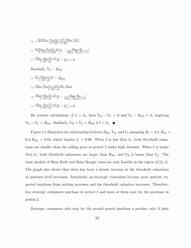
Figure 4.1 illustrates the relationship betweenRH2, VH , and VL assumingR1 = 0.5, RL2 =
0.2, RH2 = 0.65, which implies δ1 = 0.66. When δ is less then δ1, both threshold valua-
tions are smaller than the selling price in period 2 under high demand. When δ is larger
then δ1, both threshold valuations are larger than RH2, and VH is larger than VL. The
basic models of Skim Both and Skim Myopic cases are only feasible in the region of [δ1, 1].
The graph also shows that there has been a steady increase in the threshold valuations
as patience level increases. Intuitively, as strategic consumers become more patient, ex-
pected surpluses from waiting increases and the threshold valuation increases. Therefore,
less strategic consumers purchase in period 1 and more of them wait for the purchase in
period 2.
Strategic consumers who wait for the second period purchase a product only if their
23

Figure 4.1: An example of the relationship between the threshold valuation functions andselling price in period 2 under high demand for case R1 = 0.5, RL2 = 0.2, RH2 = 0.65 andδ1 = 0.66.
valuations are higher than the selling price in period 2 (≥ RL2). In accordance with
Lemma 1, when δ < δ1, VH < VL < RH2, (1 − VL) is the fraction of strategic consumers
who purchase the product in period 1. The remaining strategic consumers may buy only
when the firm charges RL2 in period 2. Under this condition, the critical valuation VH and
the price RH2 do not have any influence on strategic consumer’ purchase timing decision.
So the firm should not charge a price in period 2 that is higher than in period 1 under low
demand. So the threshold valuation VL is employed when δ < δ1.
24

We note, however, that when δ > δ1, VL > RH2, the critical value could not be cal-
culated by equation SIP = ESWL anymore due to consumers’ ability to purchase the
product at RH2. So (1 − VH) is the percentage of strategic consumers who purchase the
product in period 1, and the remain strategic consumers wait for period 2 if their base
valuations belong to [RH2, VH ]. Therefore, when Clearance Sales strategy is employed,
V =
VH δ ≥ δ1
VL δ < δ1
When Dynamic Pricing and Intermediate Supply strategies are employed,
V = VH .
4.2 Pricing Policies
In this setting, without loss of generality, we normalize p and NL to 12
and assume c is
less than 12. Retailers may practise one of two specific prices policies, depending on the
parameter interval: prices may be set to skim both types (myopic and strategic) of high
valuation consumers in period 1; or set to skim only high valuation myopic consumers
in period 1, deferring all strategic consumers to period 2. Following Mantin and Granot
(2010), we refer to these pricing policies as Skim Both (SB) pricing and Skim Myopic (SM)
pricing, respectively. Specifically, we have
Skim Both (SB): price to skim high-valuation consumers of both types in the first
period, implying V < 1.
25

Skim Myopic (SM): price to skim only high-valuation myopic consumers in the first
period. That is, none of the strategic consumers purchases in the first period; they all wait
for the second period; i.e. V = 1.
The retailer must switch from case Skim Both to case SM if V equals 1, but he may
choose to switch at an earlier stage to impose waiting on strategic consumers. We need to
derive the switching point based on the other parameters. Hence, we derive δ3, which is
obtained by solving V = 1 for δ. That is
δ3 ≡2(1−R1)
2−RH2 −RL2
(4.4)
Therefore, when δ exceeds δ3, the retailer must switch to the Skim Myopic case. The
consistency for the profit functions of Skim Both and SM will be shown later in this section.
Pictorially, the strategic consumers’ type space (valuation) is divided into four regions,
as shown in Figure 4.2, which also provides an insight for the behavior of strategic con-
sumers under Clearance Sales strategy. Strategic consumers with valuations below RL2
never purchase as their willingness to purchase is too low. For those consumers with val-
uations between RL2 and R1, the only profitable option is to wait and purchase when the
retailer sells the product for the price of RL2. Consumers with valuations above R1 act
strategically according to the threshold function V , such that a strategic consumer waits
strategically only if his or her valuation satisfies R1 < v ≤ V . Those with valuation v > V
are the buy-now strategic consumers who tend to avoid the waiting cost. Notice that part
(a) in figure 4.2 is only feasible for Skim Both up to the point where V reaches 1.
26

Figure 4.2: An example of a purchasing strategy of the strategic consumers under theClearance Sale strategy for the case δ = 0.73, c = 0.1. Note that the Skim Both case isonly feasible when V < 1 in panel (a).
27

Chapter 5
Clearance Sales Strategy
In this scenario, all leftover inventory is released into the market in the second period.
The retailer sets the price, R1, in the first period whereas the selling price in the second
period, Ri2, i ∈ {H,L}, is determined by the market. Having capacity of K units implies
that at most K units of the product will be sold during the selling season. Specifically, Di1
units are sold in the first period, and the remaining units, at most K− Di1 products are
sold in the second period. That is Di2 ≤ K −Di1. Based on the relationship between Di2
and K −Di1 and when the entire inventory is sold out, we further separate the analysis of
Clearance Sales strategy into three scenarios.
(a) If Di2 = K −Di1 ∀i and i ∈ {H,L}: inventory is depleted completely by the end
of the selling season.
(b)1 If DL2 = K −DL1 and DH1 = K: inventory is depleted completely at the end of
1Case (b) is a special case of case (a), we analyze case (b) separately to capture its specialities.
28

period 1 under high demand.
(c) If Di2 < K−Di1 ∀i and i ∈ {H,L}: some leftover inventory remains (when demand
is low) by the end of the selling season.
5.1 Case a: Inventory Depleted Completely over Two-
period Sales
Based on the information in Figure 4.2 above, we can derive the demand function of this
product under both low and high demands. Let Dφi1 denote the realized demand under
state i, i ∈ {H,L} in period t, t ∈ {1, 2}, and φ = SB, SM ; note that if φ = SM , then
V = 1. In this setting, the realized demand in period 1 at price R1 is the number of
myopic consumers with valuations above R1 plus the number of strategic consumers with
valuations above V in the Skim Both case, and only the number of myopic consumers with
valuations above R1 in the Skim Myopic case. Specifically,
Dφi1 ≡ αNi(1−R1) + (1− α)Ni(1− V ) = αNi(VH −R1) +Ni(1− V )
The realized demand in period 2 at price Ri2 is the number of strategic consumers
with valuations below V but above Ri2 in Skim Both case, and the number of strategic
consumers with valuations below 1 but above Ri2 in Skim Myopic case.
Dφi2 ≡ (1− α)Ni(V −Ri2)
Let ΠSB and ΠSM denote the retailer’s profits under Skim Both and Skim Myopic
pricing, respectively. The profit function under low demand is given by ΠL = R1DL1 +
29

RL2DL2 − cK, and under high demand is given by ΠH = R1DH1 + RH2DH2 − cK. Thus,
the retailer’s total expected profit is Π = pΠH + (1− p)ΠL.
5.1.1 Equilibrium Pricing Policies and Model Analysis
The model is solved backward to yield the subgame perfect Nash equilibrium, which al-
lows us to derive the equilibrium pricing policies. For both pricing strategies, we identify
the subgame-perfect Nash equilibrium, and show that given the retailer’s strategy, the
equilibrium in the consumer subgame is unique.
Let Rφit denote the selling price under state i, i ∈ {H,L} in period t, t ∈ {1, 2}, and
φ = SB, SM . Recalling our assumption that the retailer employs Clearance Sales strategy,
the selling prices in period 2, Ri2, are determined by the demand (the strategic consumers
who wait for the second period), and the left-over inventory (i.e. K − Di1, i ∈ {H,L}).
Thus,
(RφH2, R
φL2) = (−K−αR1+1
1−α , −2K−αR1+11−α ), φ ∈ {SB, SM}
The first period price is obtained by solving the first-order condition, which is to max-
imize the profit. For the first-order conditions, an optimal solution is
RSB1 = 2
3αKδ − 2
3Kα + 1− 3
4Kδ − 2
3K, if Skim Both is employed and
RSM1 = 1− 4
3K, if SM is employed.
Recall that the precondition of the Clearance Sale scenario is that the consumers’
threshold valuation, V , should be higher than the selling price in period 2 under high
demand; δ should be larger than δ1 to satisfy this condition (Lemma 1). Substituting the
30
price expressions in the expression of δ1 yields
δ1 =4(1− 2α)
3− 8α. (5.1)
Similarly, we get
δ3 =8(1− α)
9− 8α. (5.2)
Notice that δ1 = δ3 when α = 34.
When α ∈ [0, 0.5], δ1 equals 0 since the valuation of δ1 over the regular interval of
δ, thus the basic Skim Both and Skim Myopic models are always feasible in this interval
of α. When α ∈ (0.5, 0.75], δ1 is between 0 and 1, and the basic Skim Both and Skim
Myopic models are only feasible when δ is larger than δ1. We assume that the retailer does
not deplete all inventory in period 1 in the basic Skim Both and Skim Myopic models.
Therefore, we solve the value of α, where the retailer sell out everything in period 1. Quite
surprisingly, we find out that the retailer depletes all inventory if the proportion of myopic
consumer is equals to or over 34, and α = 3
4is also where δ1 = δ3. As a result of this fact,
retailer switch from Skim Myopic to sell everything in period 1 when α = 34. Therefore, δ1
equals 1 when α ∈ (0.75, 1].
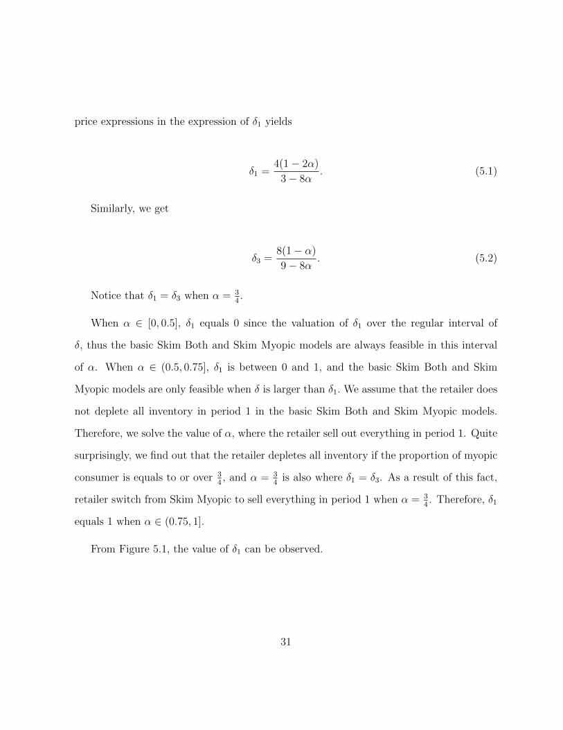
From Figure 5.1, the value of δ1 can be observed.
31

Figure 5.1: The value of δ1. When δ > δ1, the basic CS is employed by the retailer; whenδ < δ1, the retailer employs AH.
δ1 ∈
0 if α ∈ [0, 0.5]
(0, 1) if α ∈ (0.5, 0.75]
1 if α ∈ (0.75, 1]
(5.3)
Since we are more interested in the cases where V > RH2 > R1, we focus the analysis
on the feasible interval of α and δ. δ1 equals zero in the region of α ∈ [0, 0.5], which
implies that the threshold valuation is always larger than the selling price in period 2 in
32

this interval. So we always have V > RH2 > R1 when α ∈ (0, 0.5]. Basic skim both
and skim myopic cases can be applied in this interval. When α ∈ (0.5, 1), the threshold
valuation is only larger than the selling price in period 2 if δ > δ1. This may happen under
high demand and if the entire inventory is sold during the first period. A subsection named
sell all under high demand is given under this section.
In the case where all products are sold in period 1 under high demand, the selling
prices in period 2 are irrelevant anymore since no product is available in period 2. This
case is named AH, which means the retailer sells all units under high demand in period 1.
Intuitively, we know that all the sales occur in period-1 with a relatively high price if
the proportion of myopic consumers is relatively high in the market. If the proportion of
myopic consumers is over half, the retailer will not have any inventory left in period 2 under
high demand under most of the conditions, Specifically, the retailer depletes all inventory
if the proportion of myopic consumers equals or exceeds 75%.
Based on Lemma 1 and Figure 5.1, the retailer employ the basic Skim Both and Skim
Myopic models when consumers’ patience lever is less than δ1, and the retailer switches
from basic Skim Both and Skim Myopic to case AH when δ ≥ δ1 since all inventory is
depleted in period 1 of the selling season. Moreover, the retailer employs basic Skim
Myopic instead of basic Skim Both if consumers’ patience level equals or exceeds δ3. The
separation of the cases is given in Figure 5.2.
33

Figure 5.2: The case separation based on α and δ when supply equals demand, whereSB=Skim Both; SM=Skim Myopic and AH=sell All under High demand in period1. Notethat the downsloping line is δ3; the stepwise increasing curve is δ1.
5.1.2 Basic Skim Both and Skim Myopic
In the basic Skim Both and Skim Myopic cases, the retailer has some left-over inventory in
period 2 after the sales in period 1. And both RL2 and RH2 exist and are strictly positive
(0 < RL2, RH2 < 1). Later in Section 4.2, binding constraints are imposed. Naturally,
a retailer prefers Skim Both over Skim Myopic whenever ΠSB ≥ ΠSM . The retailer is
indifferent between Skim Both and Skim Myopic at δ3, where δ3 is the value of δ solved
by (V = 1), and δ = δ3, when we solve ΠSB = ΠSM in δ, finding that further proves the
34

consistency of this model. A retailer employs Skim Both when δ is less than δ3; otherwise,
the retailer is forced to switch to Skim Myopic pricing due to the strategic consumers’
behavior.
There are a few conditions that need to be satisfied in this model. First of all, we need
to satisfy the assumption of R1 < RH2, so δ4 is solved by R1 = RH2 for δ. Hence, RH2 is
larger than R1 When δ > δ4.
δ4 ≡4(1− 2α)
9− 8α=
8(1− α)− 4
9− 8α< δ3 (5.4)
Note that δ4 < δ3. Also we need to satisfy the positivity of RL2. Since RL2 is decreasing
in α, we employ α1 solved from RL2 = 0 for α. This condition will be released after the
inventory level is decided.
α1 =
12−8K−9Kδ−
√832K2−576K−624K2δ+144+168Kδ+81K2δ2
16K(1−δ) if δ1 < δ < δ3
3(1+2c)4(1+c)
if δ ≥ δ3
(5.5)
Substitute the prices in the profit functions. The corresponding profit functions are:
ΠSB = KA1
192(1−δ)(1−α), and ΠSM = K(−6α+8Kα−9K+6−6c+6cα)
6(1−α).
where A1 = K(8α−9)2δ2 +(−192+192α+16Kα−128Kα2 +192c−192cα+144K)δ+
92− 224K − 192α + 128Kα− 192c+ 64Kα2 + 192cα
Proposition 2 Consider the Clearance Sales strategy in Case (a) where δ > δ1, assuming
p = 12
and NL = 12, if α < min{α1,
34}, if δ1 < δ < δ3, then Skim Both is employed;
35

otherwise, if δ > δ3, then Skim Myopic is employed. If α ≥ 34, then the retailers always
employ Skim Myopic policy.
Proof. Recall that δ > δ1 ensures VH > VL > RH2, and recall that δ1 = 4(1−2α)3−8α
. The
retailer switches from Skim Both to Skim Myopic at δ = δ3 = 8(1−α)9−8α
.
There is not a certain relationship between δ1 and δ3. Note that δ1 = δ3 when α = 34.
If α < 34, then δ1 < δ3, both Skim Both and Skim Myopic cases exist in the market. If
α ≥ 34, then δ1 ≥ δ3, and only the Skim Myopic case is feasible.
We also need to guarantee the positivity of RL2 by limiting α < min{α, 34}. Figure 5.2
shows that if δ < δ1, the retailer deplete all inventory in period 1 and AH is employed.
Further details about case AH will be given in Section 4.2.
The profit function is quadratic in inventory level (K), and we need to find out if it is
convex or concave in K. If the profit function is convex in K, the corner solution(s) within
the feasible region will be employed, and if the profit function is concave in K, the optimal
solution within the feasible region will be chosen.
Proposition 3 Consider the Clearance Sales strategy in Case (a) where δ > δ1, assuming
p = 12
and NL = 12, the retailer’s profit function is strictly concave in the inventory quantity
stocked, thus guaranteeing an optimal stocking decision.
Proof. Under Skim Both pricing, ∂2ΠSB
∂K2 = (8α−9)2δ2+(144+16α−128α2)δ−224+128α+64α2
96(1−α)(1−δ) . The
denominator is clearly positive. The numerator can be written as f1 = aδ2+bδ+c, where f1
is convex in δ. ∂2f1∂δ2
= 2(8α−9)2 > 0 and the discriminant of f1 is ∆f1 = 1152(8α−9)2 ≥ 0.
36

Hence, f1 has two real number roots which are −4(2+3√
2+2α)9−8α
and −4(2−3√
2−2α)9−8α
, where the
former is negative and the latter is positive. Let δ5 denote the positive root. That is
δ5 ≡ −4(2−3√
2−2α)9−8α
. Since δ5 − δ3 = 4(−4+3√
2)9−8α
> 0, δ5 is larger than δ3.
Since the retailer employs Skim Both in the region of [δ1, δ3], ∂2ΠSB
∂K2 is negative in the
region of δ ∈ [0, δ3], which means that ΠSB is strictly concave in the inventory quantity
stocked.
Under Skim Myopic pricing,∂2ΠSM
∂K2 = − 9−8α3(1−α)
< 0. Hence, ΠSM is strictly concave in
the inventory quantity stocked.
The corresponding optimal stocking decision is
K =
96(1−c)(1−δ)(1−α)
−(8α−9)2δ2−(144+16α−128α2)δ+224−128α−64α2 if δ1 < δ < δ3
3(1−c)(1−α)9−8α
if δ ≥ δ3
Substituting the K in the profit function:
ΠSB = 48(1−c)2(1−δ)(1−α)−(8α−9)2δ2−(144+16α−128α2)δ+224−128α−64α2 ,
ΠSM = 3(1−α)(1−c)22(9−8α)
,
and the corresponding strategic consumer critical valuation is
V =
64c(δ−1)2α2−8(δ−1)(9δ+9cδ+16)α+72δ−160+81δ2+72cδ−64c−224+144δ+16αδ+128α−128α2δ+64α2δ2−144αδ2+81δ2+64α2 if δ1 < δ < δ
1 if δ ≥ δ3
The proposition above implies that there is always an optimal inventory level decision,
and the retailer will obtain more profit if he employs a relatively low stocking decision
to satisfy part of the demand or a relatively high stocking decision to satisfy all demand.
With a high δ, the consumers are very patient and wait for the product discounts. Let’s
37

take luxury goods as a example. If the retailer is selling luxury goods, a relatively low
stocking decision would be employed to stimulate the demand at a high selling price in
both periods. If the product is non-seasonal or non-perishable, the retailer sets a relatively
high stocking decision to sell as many units as possible at a lower rate.
Myopic consumers purchase the product if their valuations are higher than the first
period price. Intuitively, as the percentage of myopic consumers in the market increases,
more strategic consumers purchase in the second period instead of the first period due to
retailer’s pricing strategy. Recall that only the strategic consumers with valuations between
V and one purchase goods in the first period. As this critical valuation, V , increases, more
strategic consumers wait and purchase in the second period. We seek to characterize the
change in the critical valuation as more myopic consumers exist in the market.
∂V∂α
= 8(1−δ)(1−c)f2(f3)2
, where f2 = −64(9δ+ 16)(δ− 1)2α2 +α16(δ− 1)(81δ2 + 72δ− 160)−
729δ3 +2016δ−1024 and f3 is some function of α and δ, which we suppress since it is clear
that the denominator is positive. As (1 − c) and (1 − δ) are positive, so the relationship
between critical valuation and α is purely dependent on B1. B1 can be written as f2 = aα2+
bα+ c. Since the discriminant of function f2 is ∆f2 = 73728(32−9δ2)(δ−1)2 ≥ 0, function
f2 has two real number roots: −81δ2−72δ+160±12√
64−18δ2
8(9δ+16)(1−δ) . ∂2f2∂α2 = −(128(9δ+16))(δ−1)2 < 0,
so function B1 is concave in α.
Since one root is larger than 1 and the other root is less than one, we denote the smaller
root as α2: α2 ≡ −81δ2−72δ+160−12√
64−18δ2
8(9δ+16)(1−δ) , whereα2 is between 0 and 1 when δ ∈ [0, 0.578],
and α2 is less than 0 if δ ∈ [0.578, δ3]. Note that if δ ≥ δ3, Skim Myopic is employed and
V = 1.
38
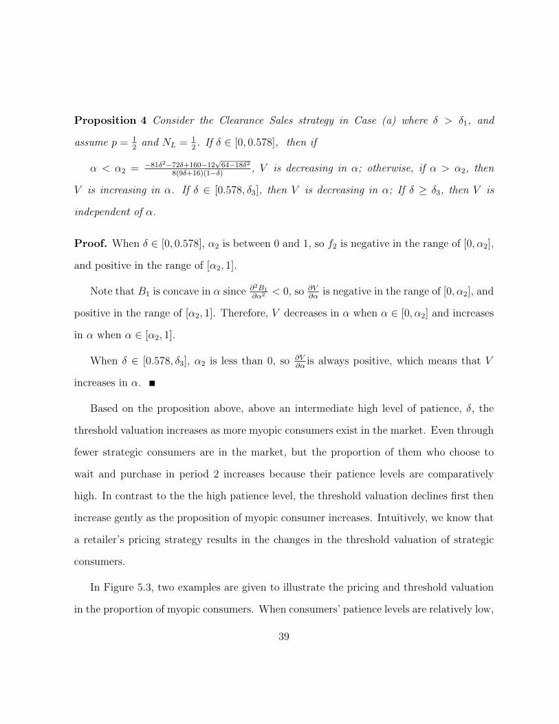
Proposition 4 Consider the Clearance Sales strategy in Case (a) where δ > δ1, and
assume p = 12
and NL = 12. If δ ∈ [0, 0.578], then if
α < α2 = −81δ2−72δ+160−12√
64−18δ2
8(9δ+16)(1−δ) , V is decreasing in α; otherwise, if α > α2, then
V is increasing in α. If δ ∈ [0.578, δ3], then V is decreasing in α; If δ ≥ δ3, then V is
independent of α.
Proof. When δ ∈ [0, 0.578], α2 is between 0 and 1, so f2 is negative in the range of [0, α2],
and positive in the range of [α2, 1].
Note that B1 is concave in α since ∂2B1
∂α2 < 0, so ∂V∂α
is negative in the range of [0, α2], and
positive in the range of [α2, 1]. Therefore, V decreases in α when α ∈ [0, α2] and increases
in α when α ∈ [α2, 1].
When δ ∈ [0.578, δ3], α2 is less than 0, so ∂V∂α
is always positive, which means that V
increases in α.
Based on the proposition above, above an intermediate high level of patience, δ, the
threshold valuation increases as more myopic consumers exist in the market. Even through
fewer strategic consumers are in the market, but the proportion of them who choose to
wait and purchase in period 2 increases because their patience levels are comparatively
high. In contrast to the the high patience level, the threshold valuation declines first then
increase gently as the proposition of myopic consumer increases. Intuitively, we know that
a retailer’s pricing strategy results in the changes in the threshold valuation of strategic
consumers.
In Figure 5.3, two examples are given to illustrate the pricing and threshold valuation
in the proportion of myopic consumers. When consumers’ patience levels are relatively low,
39

the threshold valuation decreases gently in α when α is small; then the threshold valuation
increases when α is sufficiently high in α. As shown in Figure 5.3, the selling price in
period 2 under high demand increases in α, and the selling price in period 1 decreases first
then increases in α, which explains the trend of threshold valuation above an intermediate
high level of patience level.
The retailer tries to manipulate strategic consumers’ behavior by changing selling prices.
Based on the threshold valuation, more strategic consumers purchase in period 1 as R1
decreases, and more of them decide to wait for period 2 as R1 increases, as shown in panel
(a) of Figure 5.3. As shown in panel (b), the graph shows that there is a steep rise in the
selling price in period 2 under high demand with a slight change in R1, and the selling
price in period 2 under low demand is relatively higher than what we have in panel (a).
Therefore, the threshold valuation increases steadily as more myopic consumers exist in
the market under a high patience level.
The left panel of Figure 5.3, feasible exists only when α is sufficiently small, since V
needs to be larger than RH2. However, this condition only holds if δ is larger than δ1 and
the valuation of δ1 is given in Figure 5.1, and δ1 = 4(1−2α)3−8α
. The infeasible region further
verifies the correctness of Lemma 1. Since RH2 is larger than V in the infeasible region in
the left part of Figure 5.3, the basic Clearance Sales strategy models do not work in this
region. As illustrated in Figure 5.2, the retailer sells everything in period 1 under high
demand, a scenario that fits this region. More details are given later in a section 4.13.
Quite surprisingly, numerical analysis suggests that optimal stocking and correspond-
ing profit decrease as the proportion of myopic consumers increases, which implies that
40

Figure 5.3: Examples of prices and threshold valuations under Clearance Sales strategy,and basic Skim Both and Skim Myopic cases are employed. Note that the feasible regionin panel (a) is for basic SB and the left region is feasible for AH.
strategic consumer behavior may actually benefit the retailer. This finding counters com-
mon intuition that strategic customers who consider all available purchase choices hurt
retailer’s profit. Su (2007) identified finding as the result of scarcity and the heterogeneity
of consumers. The threat of stock-outs discourages some strategic consumers from waiting,
which may also increase their willingness to pay. In our model, the valuations of consumers
are fixed, and all consumers are risk neutral. We can, however, consider the scarcity in a
different way. As more myopic consumers exist in the market, fewer products are left for
period 2, which further increases the selling price in period 2 so that fewer strategic con-
sumers have the ability to purchase. The retailer then cares less about strategic consumers
41

and defers more of them to period 2 by increasing R1 and decreasing RL2 as α increases.
With fewer strategic consumers, the retailer’s potential profit from both period 1 and pe-
riod 2 diminishes (recall that only strategic consumers may delay their purchase to the
second period). Another possible explanation for this behavior is that the retailer will
not lose the strategic consumers immediately if he charges a very high price in period 1,
and extra profit may be obtained from strategically waiting consumers if a lower price is
charged in the second period.
As the selling price in period 1 increases in α, fewer myopic consumers are capable of
purchasing in period 1 since their valuations may be lower than the selling price. However,
considering the sales lost from strategic consumers, the retailer stocks less as more myopic
consumers exist in the market. Therefore, these variations may result in a corresponding
decrease of profit in α. Cachon and Swinney (2009) also find that a firm stocks less with
strategic customers than without them in the uncertain demand case. More interestingly,
they study the additional value of quick response to mitigate the negative consequences
of strategic purchase behavior of customers.This finding has important implications for
developing the dynamic pricing theory since strategic consumers’ behavior may actually
benefit the retailer. The described trends of inventory level and profit functions are shown
in Figure 5.4 using the same parameter values as in Figure 5.3.
Proposition 5 Consider the Clearance Sales strategy in Case (a) where δ1 < δ < δ3,
assuming p = 12
and NL = 12, as myopic consumers are more numerous in the market, (i)
the capacity function K is strictly decreasing in α, which implies that as myopic consumers
are more numerous in the market, the retailer chooses a lower capacity; (ii) the retailer
42

Figure 5.4: Two examples of profits and corresponding inventory level under Basic SkimBoth and Skim Myopic cases. Note that the profit decreases to 0 when α increases to 1.Later we will see that this is not the case in equilibrium.
gets less profit in basic Skim Both and Skim Myopic cases.
Proof. In Skim Both, ∂K∂α
= −96(1−c)(1−δ)f3(f4)2
, where f4 is some function of α and δ, and
f3 = 64(δ − 1)2α2 − 128(δ − 1)2α− 160δ + 63δ2 + 96.
To show ∂K∂α
< 0, we need to proof f3 > 0. Since ∂2C1
∂α2 = 128(δ − 1)2 ≥ 0, f3 is convex
in α.
The discriminate of function f3 is ∆f3 = 256(δ2+32δ−32)(δ−1)2. Because (δ2+32δ−32)
is negative in the region of δ ∈ [0, δ3]. Recall that δ3 = 8(1−α)9−8α
which is the switching point
from Skim Both to Skim Myopic. So ∆f3 < 0.
43

Since the discriminant of function f3 is less than zero, function f3 does not have any
real roots. So function f3 is positive in the region of δ ∈ [0, δ3]. Hence, The capacity
function K is strictly decreasing in α.
Similarly, we can prove that the profit function is strictly decreasing in α.
∂ΠSB
∂α= 48(1−c)2(1−δ)f6
(f5)2, where f5 is some function of α and δ, and f6 = −64(δ − 1)2α2 −
128(δ − 1)2α− 96− 63δ2 + 160δ. Since ∂2C4
∂α2 = −128(δ − 1)2 6 0, f6 is concave.
Since the discriminant of function f6 is ∆f6 = 256(δ2 + 32δ − 32)(δ − 1)2 < 0, function
f6 does not have any real roots. So f6 is negative.
Since∂ΠSB
∂α< 0, the profit function ΠSB is strictly decreasing in α.
In Skim Myopic,∂K∂α
= − 3(1−c)(8α−9)2
< 0, and ∂ΠSM
∂α= − 3(1−c)2
2(9−8α)2< 0
Many previous studies have addressed the fact that a retailer may profit less if con-
sumers are more patient. This finding is very straightforward as we consider patience level
as a waiting cost. A high patience level implies a low waiting cost, which means the surplus
of purchasing in period 2 is still very high for strategic consumers in our model. As the
patience level increases, the threshold valuation decreases, and more strategic consumers
would like to wait and pursue a better deal in period 2. If the retailer charges RH2 under
high demand, some of the waiting strategic consumers would not purchase, which resulting
in lost sales. If the retailer charges RL2 under low demand, the potential profit for period 2
also diminishes since the waiting strategic consumers pay less to obtain the product. Thus,
a retailer gets less profit if consumer patience level increases.
Proposition 6 Consider the Clearance Sales strategy in Case (a) where δ1 < δ < δ3,
44

assuming p = 12
and NL = 12, as strategic consumers are more patient, that is, as δ
increases, the retailer’s profit decreases.
Proof. In Skim Both, ∂ΠSB
∂δ= 48(1−c)2(1−α)f8
(f7)2, where f7 is some function of α and δ, and
f8 = −(8αδ − 9δ + 8− 8α)(8αδ − 9δ − 8α + 10).
∂2f8∂δ2
= −2(9 − 8α)2 6 0, f8 is concave in δ. Since the discriminant of function f8 is
larger than 0, function f8 has two real roots: 2(5−4α)9−8α
and 8(1−α)9−8α
.
Since 2(5−4α)9−8α
> 0 and 8(1−α)9−8α
∈ [0, 1], function A is negative in the region of δ ∈ [0, 8(1−α)9−8α
]
and positive in the region of δ ∈ [8(1−α)9−8α
, 1]. Recall that δ3 = 8(1−α)9−8α
which is the switching
point from Skim Both to Skim Myopic. So Skim Both case is only applicable in the region
of δ ∈ [0, 8(1−α)9−8α
]. Therefore, ∂ΠSB
∂α< 0 in Skim Both case.
Now we plug the value of K to obtain the optimal prices.
R1 = −160+152δ−64c+128α−120αδ−8αδ2−8cδ+9δ2+136cαδ−136αδ2c−128α2δc+64α2δ2c+64cα2+72cδ2
−224+144δ+16αδ+128α−128α2δ+64α2δ2−144αδ2+81δ2+64α2
RH2 = −128α2δc+64α2δ2c+64cα2+8αδ+64α−72αδ2+8cαδ−72αδ2c+64cα+48δ+81δ2−128+96cδ−96c−224+144δ+16αδ+128α−128α2δ+64α2δ2−144αδ2+81δ2+64α2
RL2 = −128α2δc+64α2δ2c+64cα2+8αδ+64α−72αδ2+8cαδ−72αδ2c+64cα−48δ+81δ2−32+192cδ−192c−224+144δ+16αδ+128α−128α2δ+64α2δ2−144αδ2+81δ2+64α2
Usually, the selling price in period 2 is lower than the selling price in period 1 as the
retailer adopts the markdown mechanism (Lazear 1986, Smith and Achabal 1998, Gupta
et al. 2006, Zhang and Cooper 2008). Under the condition of uncertain demand, the
price that the retailer charges in the second period may be higher, or lower, than the price
posted in the first period. Specifically, if the demand in the first period is high, more of
the inventory is depleted, and with less inventory, the second period price can be higher
than the first period price. If the demand in the first period is low, all leftover inventory is
45

released in period 2. The retailer has to charge a lower price in period 2 than in period 1
to sell as much stock. The findings of the current study are consistent with those of Bitran
and Mondschein (1997), Feng and Gallego (1995), Gallego and van Ryzin (1994), who
found that prices may go either up or down over time. Possible explanations for the rise
in price are the stochastic arrival of consumers or the poisson arrivals of consumers under
continuous time and the fact that high valuation consumers arrive later during the selling
season.
Proposition 7 Consider the Clearance Sales strategy in Case (a) where δ > δ1, assuming
p = 12
and NL = 12, the selling price in period 1 is always higher than the selling price in
period 2 under low demand.
Proof. Under Skim Both case, R1 −RL2 = (1−δ)(1−c)f10f9
, where f10 = 8(δ − 1)α− 9δ + 16,
and f10 is a liner function which decreases in α. Recall that when α < min{α1 ,34},
retailers employ Skim Both if the discounting factor of consumers is between δ1 and δ3.
Since α ∈ [0, 34), function f10 is between [10 − 3δ, 16 − 9δ], function f10 is positive. f9 =
(−64α2+144α−81)δ2+(−144−16α+128α2)δ+224−128α−64α2. Since∂2f9∂δ2
= −2(8α−9)2,
f9 is concave in δ. The roots of f9 are 4(−2−2α±3√
2)9−8α
. Since one root is less than 0 and the
other root is larger than 34, function f9 is positive when α ∈ [0, 3
4). Thus, R1 > RL2 for
Skim Both cases.
Under Skim Myopic case, R1 −RL2 = 2(1−c)9−8α
> 0
The equilibrium prices for both cases are illustrated in Figure 4.2. As seen in Figure
4.2, for fixed values of δ, as α increases, the retailer increases the first period price as
46

well as the second period under high demand and decreases the second period under low
demand for both Skim Both and Skim Myopic pricing. Compared to the price curves
under Skim Both, the retailer try to increase the first period price and decrease the second
period price steeply in Skim Myopic. The retailer tries to encourage strategic consumers
to make purchases in the second period. This behavior coincides with the proposition
above. With fewer strategic consumers, the retailer’s potential profit from the second
period diminishes. Retailer cares less about strategic consumers and seeks to defer them
all to the second period, while focusing attention on first period demand stemming from
myopic consumers. Yet, the retailer stocks a lower inventory level and sets a higher first
period price (partially to divert strategic consumers to the second period). Ultimately, this
behavior results in less profit for the retailer.
In this section, so far, we have found that the second period selling price in low demand
scenario, RL2, decreases in α. Thus, as more myopic consumers exist in the market, RL2,
keeps decreasing until it reach 0. Under low demand, the retailer employs a very low selling
price in period 2 to sell all the left-over inventory. As the proportion of myopic consumers
increases in the market, more myopic consumers purchase products in period 1, and more
strategic consumers wait to purchase in period 2 as a result of the low selling price RL2.
The analysis conducted so far is not applicable any more if the selling price in period 2 is
less than 0. Cases in which the selling price in period 2 equals 0 as discussed in the next
section (4.2).
The single most striking observation to emerge from the comparison is that profit
function decreases as the number of myopic consumers increases. As mentioned, this
finding corroborates the ideas of Su (2007), who identified this as the result of scarcity
47

and heterogeneity of consumers. As more myopic consumers exist in the market, fewer
products are left for period 2, which further increases the selling price in period 2 so that
fewer strategic consumers have the ability to purchase. The retailer at this point cares
less about strategic consumers and defers more of them to period 2 by increasing R1 and
decreasing RL2 as α increases. Thus, with fewer strategic consumers, the retailer’s potential
profit from both periods 1 and 2 diminishes (recall that only strategic consumers may delay
their purchase to the second period). Another possible explanation for this finding is that
strategic waiting consumers may result in extra sales if a lower price is charged in the
second period.
5.2 Case b: Inventory Depleted Completely in pe-
riod 1 under High Demand
Recall that if either α ≤ 0.5 or δ > δ1 and α > 0.5, then VH > VL > RH2. We analyzed
this condition in the Clearance Sales strategy case. Next, we investigate what happens if
δ is less than δ1. When δ < δ1 and α > 0.5, VH < VL < RH2. The selling price under
high demand in period 2, RH2, is irrelevant at this point since the entire inventory is sold
in period 1. Therefore, the demand under high demand in period 1, DH1, is equal to the
inventory level, K, and the selling season ends right after period 1. This strategy is good
for the retailer to shorten the shelf time and save the inventory cost, which may result in
higher profit compared to the based case illustrated in Section 4.1.
Based on the analysis in section 4.12, the combining valuations of α and δ results in this
48
situation. It happens when the proportion of myopic consumers is between 50% and 75%
and the consumers’ patience level is relatively low or the proportion of myopic consumers
exceeds 75%. Since the patience level is very low for strategic consumers, and few strategic
consumers can benefit from the waiting and purchasing in period 2, the retailer can charge
a relatively low price for the product in period 1 to induce early purchases in period 1.
Since there is no second period if demand is high, VH is not relevant, and strategic
consumers consider only VL, V = VL = R1−δRL2(1−p)1−δ(1−p) . Even though the sales under high
demand is set to be equal to inventory level (K), we do not know if the retailer sells every-
thing under low demand. Hence, we still need to explore whether inventory is completely
depleted during the selling season or not.
As before, we get the corresponding demand functions under Skim Both. To distinguish
this special case from the basic ones, we call it SB-AH.
Under Low demand:
DSB-AHL1 = αNL(1−R1) + (1−α)NL(1−V ) = αNL(V −R1) +NL(1−V ) and DSB-AH
L2 =
(1− α)NL(V −RL2).
Under high demand:
DSB-AHH1 = K and DSB−AH
H2 = 0.
The profit function under low demand is given by ΠSB−AHL = R1DL1 + RL2DL2 − cK,
and under high demand is ΠSB-AHH = R1DH1−cK. Thus, the retailer’s total expected profit
is ΠSB-AH = p · ΠH + (1− p) · ΠL.
Recalling that we assume that the retailer employs Clearance Sales strategy, the selling
49

price in period 2, RL2, is determined by the demand and the leftover inventory (i.e.,
K = DL1 +DL2). Specifically, RL2 = −2K−αR1+11−α
Since the inventory is sold completely in period 1 if demand is high, the selling price in
period 2, R1, is also determined by the demand and the leftover inventory (i.e., K = DH1).
Thus, R1 = −K − 12Kδ + 1.
The model is solved backward to yield the subgame perfect Nash equilibrium, which
allows us to derive the equilibrium pricing policies. We identify subgame-perfect Nash
equilibrium and show that, given the retailer’s strategy, the equilibrium in the consumer
subgame is unique.
The profit function is by:
ΠSB-AH = K(−10K−3Kδ+8+8Kα+4αKδ−8α−8c+8cα)8(1−α)
.
Based on the profit function above, the profit function is concave in K, there is always
an optimal inventory level exist.
Proposition 8 Consider the Clearance Sales strategy in Case SB-AH where δ ≤ δ1, as-
suming p = 12
and NL = 12, where SB-AH is employed, the retailer’s profit function is
strictly concave in the inventory quantity stocked.
Proof. In SB-AH case,∂2ΠSB-AH
∂K2 = − (8+4δ)α−10−3δ4(1−α)
. The denominator is positive since
α ∈ (0.5, 1). And the numerator is strictly increasing in α; when α = 0.5, the numerator
= −6 − δ < 0, and when α = 1, the numerator= −2 + δ < 0. Thus, the numerator is
negative, ∂2ΠSB-AH
∂K2 < 0. So ∂2ΠSB-AH
∂K2 is negative and the profit function is strictly concave
in K.
50

The corresponding optimal stocking decision is K = KSB-AH ≡ 4(1−c))(1−α)10+3δ−8α−4αδ
.
Substituting theK in the profit function: ΠSB-AH = 2(c−1)2(1−α)10+3δ−8α−4αδ
, and the corresponding
prices and threshold valuation are
(R1, RL2) = (−4c+4cα−6+4α−2cδ+2cαδ−δ+2αδ−10−3δ+8α+4αδ
, −2−3δ+4α+2αδ−8c+4cα+2cαδ−10−3δ+8α+4αδ
);
V = −3δ+2αδ+2cαδ−4c+4cα−6+4α−10−3δ+8α+4αδ
.
Proposition 9 Consider the Clearance Sales strategy where δ ≤ δ1, assuming p = 12
and
NL = 12, as myopic consumers are more numerous in the market, (i) the capacity function
K is strictly decreasing in α, which implies that as myopic consumers are more numerous
in the market, the retailer chooses a lower capacity; (ii) the retailer gets less profit in case
SB-AH.
Proof. Follows immediately from ∂ΠSB-AH
∂α= − 2(1−c)2(2−δ)
(−10−3δ+8α+4αδ)2< 0
and ∂KSB-AH
∂α= − 4(1−c)(2−δ)
(−10−3δ+8α+4αδ)2< 0
However, the retailer cannot always take the optimal stocking decision for K since the
retailer may switch to Skim Myopic, or RL2 may reach zero as α increases; and either of
them may happen first. The next step is to analyze the switching points under this case
where all products are sold in period 1 under high demand.
When RL2 = 0, KSB-AH-RL ≡ 2(1−α)−4+2α+αδ
. In this case, the inventory decision is equal to
the true demand so that the retailer does not have any leftovers, and it is denoted as SB-
AH-RL for skim both case and SM-AH-RL for skim myopic case. The inventory decision
should be equal to the smaller of KSB-AH and KSB-AH-RL for feasibility. Let α3 denote the
51

value of α which solves KSB-AH = KSB-AH-RL, and α3 ≡ 2+3δ+8c2(2+δ+2c+cδ)
> 0.5. KSB-AH is less
than KSB-AH-RL when α < α3, so α3 is the value of α for the switching point of RL2 = 0.
Let α4 denote the value of α which solves V = 1, and α4 = 22+δ
> 0.5. We need to
compare α3 and α4 to learn the switching sequence.
α3−α4 = 3δ−2+4c2(2+δ)(1+c)
can be either positive or negative, so there is no fixed relationship
between α3 and α4. When α3 < α4, the retailer switches from SB-AH to SB-AH-RL then
SM-AH-RL as α increases. When α3 > α4, V reaches 1 before RL2 becomes 0, and the
retailer switches from SB-AH to Skim myopic when he sells everything under high demand
in period 1, which is denoted as SM-AH; then he switches from SM-AH back to SM-AH-RL.
Let δa denote the value of δ which solves α3 = α4, and δa ≡ 23− 4
3c. The switching
sequence is listed below as α increases.δ ≤ δa SB-AH→ SB-AH-RL→ SM-AH-RL
δ > δa SB-AH→ SM-AH→ SM-AH-RL
There is a significant difference between the two conditions, which is demonstrated in
more in detail in the next two subsections.
5.2.1 The Switching Sequence When δ ≤ δa
Case SB-AH-RL
When δ ≤ δa, K = KSB-AH-RL if α > α3. So all demand functions are the same as in
SB-AH. The only difference between SB-AH and SB-AH-RL is the inventory decision.
Substituting K in the profit function, ΠSB-AH-RL = (1−α)(6−3δ−16c+8cα+4cαδ)2(−4+2α+αδ)2
.
52
The corresponding prices functions and threshold valuation function are (R1, RL2) =
( 2−δ4−2α−αδ , 0) and V = 2
4−2α−αδ .
Solving V = 1 in α, we have α = 22+δ
= α4, so when α > α4, the retailer switches from
SB-AH-RL to SM-AH-RL.
Proposition 10 Consider the Clearance Sales strategy where δ ≤ min{δ1, δa} and α3 ≤
α ≤ α4, assuming p = 12
and NL = 12, as more myopic consumers exist in the market,
(i) the capacity function K is strictly decreasing in α, which implies that as more myopic
consumers exist in the market, the retailer chooses a lower capacity; (ii) the retailer gets
less profit in SB-AH-RL case.
Proof. ∂KSB-AH-RL
∂α= − 2(2−δ)
(−4+2α+αδ)2< 0
∂ΠSB-AH-RL
∂α= − (2−δ)f11
2(4−2α−αδ)3 , where f11 = (3δ + 4cδ + 6 + 8c)α− 6δ − 16c.
The denominator is positive since 4 > 2α− αδ.
f11 is increasing in α, and solve f11 in α, αi ≡ 2(3δ+8c)3δ+4cδ+6+8c
. Recall that SB-AH-RL can
be implemented only if α > α3. Since α3 − α5 = 3(2−δ)2(2+δ)(3+4c)(1+c)
> 0, α3 > α5. Therefore,
f11 is positive when α > α3, so∂ΠSBRL
∂α< 0.
Case SM-AH-RL
Since the retailer switches from SB-AH-RL to SM-AH-RL, the inventory decision is still
RL2 = 0, and only myopic consumers decide to purchase in period 1, so the threshold val-
uation (V ) is 1. The profits function remains the same and the updated demand functions
are listed below.
53

Under low demand:
DSM-AH-RLL1 = αNL(1−R1) and DSM-AH-RL
L2 = (1− α)NL(1−RL2).
Under high demand:
DSM-AH-RLH1 = K2 and DSM-AH-RL
H2 = 0.
As before, the selling price in period 2, RL2, is determined by the demand and the
leftover inventory (i.e., K = DL1 +DL2).
RL2 = −2K−αR1+11−α
Since the entire inventory is sold completely in period 1 if demand is high, the selling
price in period 2, R1, is also determined by the demand and the leftover inventory (i.e.,
K = DH1). Thus, R1 = α−Kα.
The profit function is given by:
ΠSM-AH-RL = (−3K+2Kα+4α−4α2−4cα+4cα2)K4(1−α)α
.
Recall that all products are sold during the selling season and RL2 = 0. So KSM-AH-RL ≡
1− α, which is solved from RL2 = 0.
Substituting K in the profit function, ΠSM-AH-RL = (1−α)(−3+6α−4cα)4α
. And the corre-
sponding prices are (R1, RL2) = (−1+2αα
, 0).
Proposition 11 Consider the Clearance Sales strategy where δ ≤ min{δ1, δa} and α >
α4, assuming p = 12
and NL = 12, as more myopic consumers exist in the market, (i)
the capacity function K is strictly decreasing in α, which implies that as more myopic
consumers exist in the market, the retailer chooses a lower capacity; (ii) the retailer gets
less profit in SM-AH-RL case.
54

Proof. ∂KSM-AH-RL
∂α= −1 < 0
∂ΠSM-AH-RL
∂α= f12
4α2 , where f12 = −6α2 + 3 + 4cα2, and f12 is concave in α.
Solve f12 in α, and we get α = ± 3√18−12c
. So f12 is positive when α ∈ [0, 3√18−12c
], and
negative when α ∈ ( 3√18−12c
, 1].
Recall that SM-AH-RL can be implemented only if α > α4 and δ > δa. Recall that
α4 = 22+δ
and δa = 23− 4
3c, so α > 3
4−2c
Since 4 − 2c <√
18− 12c, so 34−2c
> 3√18−12c
. Thus, A is always negative when α ∈
( 34−2c
, 1]. Therefore,∂ΠSBRL
∂α< 0.
Figure 5.5: Optimal pricing policy and inventory level under Clearance Sale assuming AHis employed; δ = 0.35, c = 0.2. Note that the profit decreases to 0 as α increases to 1,which is unlikely to be optimal.
When c equals to 0.1, δa = 23− 4
3c |c=0.1= 0.4. If the patience level is evaluated as 0.35
55

which is lower than δa, the selling price in period 2 under low demand decreases to zero
before the threshold valuation reaches one. Therefore, the retailer employs SB-AH when α
is between 0 and α3; SB-AH-RL is adopted when α falls into the interval of [α3, α4]; SM-
AH-RL is employed when α is larger than α4. The results obtained from the preliminary
analysis of case AH are shown in Figure 5.5. As can be seen from the Figure 5.5 below,
only the selling prices under low demand is given for period 2 since all products are sold
in period 1 under high demand.
There are clear trends of decreasing inventory level and profit function as the propor-
tion of myopic consumer increases in Figure 5.5. The observed correlation between α and
inventory level, K, might be explained in this way. Since all products are sold in period 1
under high demand, strategic consumers only have two options left: purchase in period 1 or
purchase in period 2 only when demand is low. More strategic consumers will consequently
consider purchasing in period 1. However, the consumer’s patience level is at an intermedi-
ate low level. Intuitively, the threshold valuation is lower than the one in basic Skim Both
and Skim Myopic cases. As more myopic consumers exist in the market, more products
will be sold in period-1, leading to even fewer units left for period 2. Since the demand in
period 1 is increasing, the selling price in period 1 is relatively high and increasing in α,
which limits the demand in period 1. The total demand therefore decreases as α increases.
Even though the selling price in period 1 is higher as α increases, the extra incomes on
products sold in period 1 is not going to compensate for sales lost because of the quantity
of multi-units of strategic consumers. It is possible to hypothesis that these conditions
cause the declining profit function trend when myopic consumers are more numerous in
the market.
56

5.2.2 The Switching Sequence When δ > δa
SM-AH
When δ > δa, we switch from SB-AH directly to SM-AH while the selling price in period 2
under low demand, RL2, is strictly positive. The switching point between SB-AH and
SM-AH is solved from ΠSB-AH = ΠSM-AH, which is happen to be the same one as the one
solved rom V SB-AH = 1. So the switching point in α is α4.
The demand functions are the same as in case SB-AH, but substituting V as 1. The
profit function under low demand is given by ΠSM-AHL = R1DL1 + RL2DL2 − cK, and
under high demand is ΠSM-AHH = R1DH1 − cK. Thus, the retailer’s total expected profit is
ΠSM-AH = pΠH + (1− p)ΠL.
As the process done in case SB-AH, we get RL2 = −2K−αR1+11−α and R1 = α−K
α. The profit
function is ΠSM-AH = (−3K+2Kα+4α−4α2−4cα+4cα2)K4(1−α)α
. Based on the profit function above, the
profit function is concave in K, so there is always an optimal inventory level exist.
Proposition 12 Consider the Clearance Sales strategy where δa < δ < δ1 and α > 0.5,
, assuming p = 12
and NL = 12, the retailer’s profit function is strictly concave in the
inventory quantity stocked, which guarantees an optimal stocking decision in SM-AH case.
Proof. ∂2ΠSM-AH
∂K2 = − 3−2α2(1−α)α
< 0.
So∂2ΠSM-AH
∂K2 is negative and the profit function is strictly concave in K.
The corresponding optimal stocking decision is KSM-AH ≡ 2(1−c)(1−α)α3−2α
.
57

Substituting K in the profit function, ΠSM-AH = α(1−α)(c−1)2
3−2c, and the corresponding
prices and threshold valuation are (R1, RL2) = (1+2c−2cα3−2α
, −4α+2cα+33−2α
) and V = 1.
Proposition 13 Consider the Clearance Sales strategy where δa < δ < δ1 and α > 0.5,
assuming p = 12
and NL = 12, as more myopic consumers exist in the market, (i) the capac-
ity function K is strictly decreasing in α, which implies that as more myopic consumers
exist in the market, the retailer chooses a lower capacity; (ii) the retailer gets less profit in
the SM-AH case.
Proof. ∂KSM-AH
∂α= 2(1−c)(2α2−6α+3)
(−3+2α)2< 0.
∂ΠSM-AH
∂α= f13(1−c)2
(3−2α)2, where f13 = (2α2 − 6α+ 3), and f13 is convex in α. Solve f13 in α,
and we get α ≡ (2.366, 0.6340). Recall that the precondition of SM-AH is α > α4 = 22+δ
and α4 >23. So f13 is negative when α ∈ [α4, 1]. So ∂ΠSM-AH
∂α< 0.
When δ > δa, the switching point between SM-AH and SM-AH-RL is derived from the
of selling price function in period 2 under low demand in case SM-AH. By solving RL2 = 0
in α, we have α5 ≡ 32(2−c) .
When c is equal to 0.1, δa is 0.4. If the patience level is evaluated as 0.7 which is
larger than δa, the threshold valuation reaches 1 before the selling price in period2 under
low demand decreases to 0. The retailer employs SB-AH when α is between 0 and α4;
SM-AH is adopted when α falls into the interval of [α4, α5]; SM-AH-RL is employed when
α is larger than α5. The results obtained from the preliminary analysis of case AH are
shown in Figure 5.6. Similar to Figure 5.5, only selling price under low demand is given
for period 2 in Figure 5.6 since all products are sold in period 1 under high demand.
58

Figure 5.6: Optimal pricing policy and inventory level under Clearance Sale assuming AHis employed; δ = 0.7, c = 0.2.
There are also clear trends of decreasing inventory level and profit function as the
proportion of myopic consumer increases in Figure 5.6. The observed correlation between
α and inventory level, K, follow the same arguments as in the previous segment of switches
since they are both under case AH.
Next, we state the relationship between the patience level and retailer’s profit function.
Intuitively, we know that the profit should decrease if strategic consumers are more patient
since they have a higher chance to wait and purchase in period 2, but still satisfy with
their purchases.
Proposition 14 Consider the Clearance Sales strategy in Case (b) where δa < δ < δ1 and
α > 0.5, assuming p = 12
and NL = 12, as strategic consumers are more patient in case
59

AH, (i) the retailer either gets less profit under Skim Both cases; (ii) the retailer’s profit
is irrelevant in in δ under Skim Myopic cases.
Proof. In SB-AH,∂ΠSB−AH
∂δ= −2(c−1)2(3−4α)(1−α)
(−10−3δ+8α+4αδ)2< 0.
In SB-AH-RL, ∂ΠSB−AH−RL
∂δ= (1−α)f14
2(4−2α−αδ)3 , and the denominator is positive since 4 >
2α− αδ.
f14 = −12 + (8c+ 4cδ)α2 + (18− 3δ − 16c)α, solve f14 in α, the roots are
−18+3δ+16c±√
324−108δ−192c+9δ2+288cδ+256c2
8(2+δ)c. One root is negative and the other is between
0 and 1. Let’s demote the positive root.
That is α6 = −18+3δ+16c+√
324−108δ−192c+9δ2+288cδ+256c2
8(2+δ)c. Recall that the precondition of
SBRL is α > α3. Since α3 − α6 > 0, α3 > α6. Therefore, f14 is negative when α > α3. So
∂ΠSB−AH−RL
∂δ< 0.
In SM-AH-RL, ∂ΠSM−AH−RL
∂δ= 0. In SM-AH, ∂ΠSM−AH
∂δ= 0.
profit function is therefore irrelevant in δ in SM-AH-RL and SM-AH cases.
The analysis has so far focused on the cases where supply was completely depleted. We
have noticed that this issue as the selling price in period 1, R1, is equal to the consumer’s
maximum willingness to pay, no consumers purchase in the first period when all consumers
are myopic. Also, the retailer charges a price as 0 in period 2. Therefore, the retailer ends
up in getting zero profit when all consumers in the market are myopic. The model where
supply exceeds demand fills in the gap to resolve the problem.
60

5.3 Case c: Possible Leftover Inventory after Clear-
ance Sales
If Di2 < K − Di1, supply exceeds demand and some inventory remains after the selling
season. This case is named after supply exceeds demand, denoted as SD. The demand
functions for both Skim Both and Skim Myopic cases are the same as in the basic Skim
Both and Skim Myopic models in section 4.12.
Since supply exceeds demand when demand is low, the selling price in period 2 under
low demand is zero if the retailer releases all the inventory.
Recalling that under Clearance Sales strategy, the selling price in period 2 under high
demand, Rh2, is determined by the demand and the leftover inventory (i.e., K = Dh1+Dh2).
We have (RSB-SDH2 , RSB-SD
L2 ) = (−K−αR1+11−α , 0) and (RSB-SM
H2 , RSB-SML2 ) = (−K−αR1+1
1−α , 0).
The selling price in period 1 is obtained from the first-order condition, which is to
maximize the profit. For the first-order conditions, an optimal solution is
RSB-SD1 = −αδ−2α+7αKδ−4αK−3δ+10−3Kδ−4K
2(−3αδ−2α+α2δ+6)and RSB-SM
1 = 5−α−4K2(3−α)
.
The profit functions are ΠSB-SD = A2
32(1−δ)(3αδ+2α−α2δ−6)and
ΠSM-SD = −α2+α+16cKα+24K−24K2−48cK16(3−α)
, where A2 = −4+12αKδ−112K+4α+16αK+
12δ−12αδ+ 132Kδ−64cKα−192cKδ+ 80K2 + 192cK−72K2δ−32cKαδ−32cKα2δ2 +
32cKα2δ+96cKαδ2−30αKδ2−72αK2δ+57αK2δ2−9δ2 +9αδ2−18Kδ2−9K2δ2 +16K2α
Based on the profit function above, the profit function is concave in K, so there is
always an optimal inventory level exist.
61

Proposition 15 Consider the Clearance Sales strategy, assuming p = 12
and NL = 12,
the retailer’s profit function is strictly concave in the inventory quantity stocked, which
guarantees an optimal stocking decision under case SD.
Proof. Under Skim Both pricing, ∂2ΠSB−SD
∂K2 = −57αδ2−72αδ+16α−9δ2−72δ+8016(3−α)(1−δ)(2−αδ) , where the de-
nominator is positive.
The numerator can be written as f15 = aδ2 + bδ+ c. Since ∂2f15∂δ2
is 114α− 18 > 0 when
α > 0.2, function f15 is convex. The discriminant of f15 is ∆f15 = 384(7− 4α)(3− α) > 0,
f15 has two real number roots, which are 4(9+9α+√
126−114α+24α2)3(−3+19α)
and 4(9+9α−√
126−114α+24α2)3(−3+19α)
.
The two roots are both larger than 1 when α > 0.2. So function f15 is positive. Therefore,
function ∂2ΠSB−SD
∂K2 is negative, which means that ΠSB is strictly concave in the inventory
quantity stocked.
Under Skim Myopic pricing,∂2ΠSM−SD
∂K2 = − 33(1−α)
< 0
The corresponding optimal stocking decision is
K =
(16α2δ2−16α2δ−48αδ2+16αδ+32α+96δ−96)c+15αδ2−6αδ−8α+9δ2−66δ+56
57αδ2−72αδ+16α−9δ2−72δ+80if δ < δ3
13cα− c+ 1
2otherwise.
Substituting K in the profit function, we have
ΠSB-SD = (24αδ2−8αδ+8α2δ+48−48δ−8α2δ2−16α)c2+(−56−9δ2+6αδ+66δ−15αδ2+8α)c−27δ+9δ2+1857αδ2−72αδ+16α−9δ2−72δ+80
and ΠSM-SD = −16c2α + 1
16α + 1
8− 1
2c+ 1
2c2,
and the corresponding strategic consumer critical valuation is
V =
36cαδ2−9δ2−72cαδ−36δ−24cδ+48+32cα+32c
57αδ2−72αδ+16α−9δ2−72δ+80if α < αx
1 otherwise.
62

αx is solve from ΠSB-SD = ΠSM-SD in α.
And α7 ≡ 4(6cδ−9δ−8c+8)36cδ2−57δ2−72cδ+72δ+32c−16
The model should satisfy the condition, which is that supply exceeds demand. We
therefore need to test whether the inventory level, K, is larger or equal to the actual sales
under low demand. By solving DSB−SDL1 +DSB−SD
L2 = K in α, we get α8 ≡ A3
16c(11δ2−15δ+4).
A3 = 120cδ2 +3δ2−24cδ+12δ−96c−16+(256−112128c2δ+33792c2−1024c−384δ−
8784cδ4 + 21504cδ − 48512cδ2 + 36816cδ3 + 9δ4 + 14400c2δ4 − 73344c2δ3 + 137280c2δ2 +
48δ2 + 72δ3)12
So case SB-SD is only feasible when the proportion of myopic consumers is larger than
α8. Similarly, we solve DSML1 +DSM
L2 = K in α, and get α9 ≡ 12c3+8c
. Hence, the case SM-SD
is only feasible when the proportion of myopic consumer is larger than α9.
Proposition 16 Consider the Clearance Sales strategy where α > α8 in Skim Both and
α > α9 in Skim Myopic, assuming p = 12
and NL = 12, as more myopic consumers exist
in the market, (i) the capacity function K is strictly increasing in α, which implies that as
more myopic consumers exist in the market, the retailer chooses a lower capacity; (ii) the
retailer gets more profit in SD case.
Proof. ∂KSB−SD
∂α= 1
16− 1
6c2 > 0 since c ∈ [0, 0.5].
∂ΠSB−SD
∂α= (1−δ)f16
(57αδ2−72αδ+16α−9δ2−72δ+80)2where f16 = (456c2δ3 − 576c2δ2 + 128c2δ)α2 +
(−144c2δ3−1152c2δ2 +1280c2δ)α+513δ3 +2688c2δ−648cδ3 +216c2δ3−3648cδ+2736cδ2−
864c2δ2 − 288− 2048c2 − 1674δ2 + 1440δ + 1536c
63

Since ∂2f16∂α2 = 16c2δ(57δ2 − 72δ + 16), ∂2K
∂α2 > 0 when δ ∈ [0, 1219− 8
57
√6] and ∂2A
∂α2 < 0
when δ ∈ (1219− 8
57
√6, 12
19+ 8
57
√6].
Function f16 is convex when δ ∈ [0, 1219− 8
57
√6] and function f16 is concave when
δ ∈ (1219− 8
57
√6, 12
19+ 8
57
√6]. The two roots of function f16 solved in α are both negative
when δ ∈ [0, 1219− 8
57
√6]. When δ ∈ (12
19− 8
57
√6, 12
19+ 8
57
√6], one root is positive and the
other is negative. Thus, function f16 is always positive. And ∂ΠSB−SD
∂α> 0.
∂KSM−SD
∂α= 1
16− 1
6c2 > 0 since c ∈ [0, 0.5].
∂ΠSM−SD
∂α= c
3> 0.
Figure 5.7 shows how prices, inventory levels and corresponding profits change as the
proportion of myopic consumers increases under the Clearance Sale strategy where supply
exceeds demand. In this figure, we can also notice that the threshold valuation is higher
than the selling price in period 2 under high demand (RH2). Note that RH2 > R1 > RL2
under SD. The graph shows that prices steady increases as the proportion of myopic
consumer increases in the Skim Both cases, whereas the prices are irrelevant with α in
the Skim Myopic case. The cause of this difference is the adoption of a different pricing
policies. Recall that the retailer sells all inventory during the selling season if the demand
level is high and sells the leftover in the price of 0 in period 2 under low demand level since
supply exceeds demand in the second period.
The intuition for the increasing prices in α is straightforward. When more myopic
consumers exist in the market, more consumer will purchase in period 1 which improve
the competition between consumers for available inventory units. In Skim Myopic cases,
all strategic consumers wait to purchase in period 2 and they either pay a higher price
64

compared to period 1 or get the product for free. This situation happens when the pro-
portion of myopic consumers is relatively high in the market, so when α is high enough,
the retailer manipulates prices to defer all strategic consumers to period 2 and charges a
constant price in this interval of α to capture the profit from strategic consumers.
Interestingly, some strategic consumers purchase in period 1 under Skim Both case even
though they know that they have the chance to get the product in period 2 for free if the
demand level is low. Those strategic consumers do so to avoid the risk of purchasing the
product in a much higher price in period 2 under high demand, which is a logical and
reasonable strategy.
Figure 5.7: Optimal pricing policy and inventory level under Clearance Sale assuming SDis employed; δ = 0.6, c = 0.2.
Compared with the analysis in basic Skim Both and Skim Myopic as well as AH, the
65

analysis conducted in this section can let the retailer obtain more profit if the proportion
of myopic consumers is high in the market. The proposition above proves that the profit
function is strictly increasing in α. In Skim Both, the inventory stocked by the retailer
barely changes as α increases, however, the prices is steady increasing as the myopic con-
sumers are more numerous in the market. Therefore, the retailer obtains more profit as α
increases in Skim Both case. By analyzing the Skim Myopic only, we know that the retailer
will isolate myopic consumers from strategic consumers so that he can price differently for
the two groups. Therefore, the retailer can capture the profit from both groups by pricing
discrimination.
Proposition 17 Consider the Clearance Sales strategy in Case (c) where α > αy in Skim
Both and α > αZ in Skim Myopic, assuming p = 12
and NL = 12, as strategic consumers
are more patient when supply exceeds demand, (i) the retailer gets less profit under Skim
Both case; (ii) the retailer’s profit is irrelevant in δ under Skim Myopic case.
Proof. In Skim Both,∂ΠSB−SD
∂δ= − (1−α)f17
(f18)2,where f18 is a function of α and δ , and
f17 = (20cαδ − 16cα− 36 + 16c+ 33δ − 24cδ)(6cαδ − 8cα− 24 + 24c+ 27δ − 18cδ).
Since∂2f17∂α2 = 2(20cδ − 16c)(6cδ − 8c) > 0, f17 is convex. Since the discriminant of
function f17 is larger than 0, function f17 has two same real roots which are
(36−16c−33δ+24cδ4(5δ−4)c
, 3(8−8c−9δ+6cδ)2(3δ−4)c
). Both roots are less than zero, so function f17 is positive.
Therefore, ∂ΠSB−SD
∂δ< 0 in Skim Both case.
In Skim Myopic,∂ΠSB−SD
∂δ= 0, so profit function is irrelevant in δ under Skim Myopic
case.
66

How the profit changes as consumer’s patience level increases is demonstrated in the
proposition above. The retailer will lose profit if the patience level of strategic consumers
increases under Skim Both cases.
5.4 Summary of Clearance Sale Strategy
Three parts of the Clearance Sale strategy have been analyzed separately in the previous
sections. It would be hard to interpret the models and pricing policy separately. Thus,
we need to combine the different elements of the Clearance Sale strategy to draw a full
picture of it. However, with different combination of parameter valuations for α, δ, and
c, caution must be applied, as different models may be feasible in the same range and the
optimal one with higher profit should be chosen by the retailer. Since it is hard to analyze
the model based on parameter ranges, numerical examples are give below.
The first example is given in δ = 0.35 and c = 0.2 in Figure 5.8. As discussed above, we
know that basic Skim Both and Skim Myopic, SB-AH→SB-AH-RL→SM-AH-RL under
AH and SD models are feasible in this region of parameters. By comparing the profit
functions of those models, the dominated ones are employed based on different intervals
of α. As shown in Figure 5.8 when δ = 0.35 and c = 0.2, the basic Skim Both model is
adopted when less than 0.56 of consumers are myopic. When the proportion of myopic
consumers is between 0.56 and 0.64, the retailer employs the model of SB-AH to sell
everything in period 1 under high demand since over half consumers in the market are
myopic and strategic consumer’s patience level is relatively low. When the proportion of
myopic consumers is sufficiently high (above 0.64 in this instance), the Skim Both model
67

Figure 5.8: An example of combination of Clearance Sale strategy in the case of δ =0.35, c = 0.2.
under SD strategy will be adopted. The retailer stocks much more inventory compared to
the basic Skim Both and SB-AH and charges a lower price in both periods to capture less
profit from individual consumers, but sells much more stock.
Now, let us increase the strategic consumers’ patience level to δ = 0.7. This case is
illustrated in Figure 5.9. Following analysis steps similar to those in the last example, we
find that the best choice for the retailer when α is small is still basic Skim Both. However,
the retailer should switch from basic Skim Both into Skim Myopic directly if α is larger
than 0.7.
Numerically, the two combinations of choices for the retailer mostly dominate all pa-
rameter intervals. One may notice that the trends of inventory levels under sufficiently
68

Figure 5.9: An example of combination of Clearance Sale strategy in the case of δ =0.7, c = 0.2.
high α are different in Figures 5.8 and 5.9. At intermediate low level of δ (δ = 0.35), K
decreases in α when supply exceeds demand. Moreover, the retailer uses SB-SD under this
parameter level. As more myopic consumers exist in the market, fewer and fewer strategic
consumers will wait for period 2 since delta is not high, and retailer keeps less inventory
to save the inventory cost. And retailer can also charge a higher price within a limited
inventory level to capture higher profit. However, when δ equals to 0.7, K is increasing in
α because the retailer employs Skim Myopic. All strategic consumers wait for period 2.
Even though sales number (realized demand) in period 2 is decreasing in α. But the sales
number in the first period is significantly increasing in α. Also the prices are irrelevant
69

with alpha in Skim Myopic. That is why retailer has an increasing K in α when patience
level is high.
Consider the cases of basic SB/SM and AH under the Clearance Sales strategy, the
retailer’s profit function is strictly concave in the inventory quantity stocked. which guar-
antee an optimal inventory decision. Also the capacity function K is strictly decreasing in
α, which implies that as myopic consumers are more numerous in the market, the retailer
chooses a lower capacity. Also, as the proportion of myopic consumers increases in the
market, the retailer gets less profit. As we stated before, this finding counters common
intuition that strategic customers who consider all available purchase choices hurt retailer’s
profit. Su (2007) identified finding as the result of scarcity and the heterogeneity of con-
sumers. In our model, with fewer strategic consumers, the retailer’s potential profit from
both period 1 and period 2 diminishes.
Another possible explanation for this behavior is that the retailer will not lose the
strategic consumers immediately if he charges a very high price in period 1, and extra
profit may be obtained from strategically waiting consumers if a lower price is charged in
the second period. Considering the sales lost from strategic consumers, the retailer stocks
less as more myopic consumers exist in the market. Therefore, these variations may result
in a corresponding decrease of profit in α. Cachon and Swinney (2009) also find that
a firm stocks less with strategic customers than without them in the uncertain demand
case. This finding has important implications for developing the dynamic pricing theory
since strategic consumers’ behavior may actually benefit the retailer. We note that in the
cases of basic SB/SM and AH, the retailer ends getting zero profit when all consumers are
myopic. This seems unlikely the optimal case, which also leads us to the case SD.
70

In Skim Both case, the inventory stocked by the retailer barely changes as α increases,
however, the prices is steady increasing as the myopic consumers are more numerous in
the market. Therefore, the retailer obtains more profit as α increases in Skim Both case.
By analyzing the Skim Myopic only, we know that the retailer will isolate myopic con-
sumers from the strategic consumers so that he can price differently for those two groups.
Therefore, the retailer can capture the profit from both part by pricing discrimination.
Case SB-SD is only feasible when the proportion of myopic consumer is larger than
α8. Similarly, the case SM-SD is only feasible when the proportion of myopic consumer is
larger than α9. Therefore, the retailer only consider the basic SB/SM and AH when α is
relatively small. Moreover, if basic SB/SM or AH models is employed, the retailer obtains
zero profit when all consumers are myopic. The retailer has to adopt SD to profit. Then
we know a switch must occur for a certain value of α, hence up to this value of α, retailer’s
profit decreases in α, thereafter his profit increases in α.
As strategic consumers are more patient in cases of basic Skim Both and Skim Myopic,
the retailer’s profit strictly decreases. However, as strategic consumers are more patient in
cases of AH and SD, the retailer gets less profit under Skim Both cases and the retailer’s
profit is irrelevant in in δ under Skim Myopic cases. The retailer isolates myopic consumers
from the strategic consumers in Skim Myopic so that he can price differently for those two
groups. The retailer ignores strategic consumers’ patience level when he makes the pricing
decisions. Hence, the profit function is irrelevant with δ.
71

Chapter 6
Optimal Release Strategy
In the previous section, the Clearance Sales strategy was studied in isolation. In this
section, we assume that Clearance Sales strategy is one available inventory release strategy
among other options. To find out the optimal release strategy, we study the Dynamic
Pricing strategy and Intermediate Supply strategy in this section. Of the three strategies,
the prevailing optimal release strategy is the one that maximizes the retailer’s profit.
6.1 Dynamic Pricing Strategy
In this setting, the retailer ignores capacity constraints during the second period of the
selling horizon and determines an original inventory ,K, that can satisfies the demand
under both NH and NL. However, after the first period demand is realized, the left-over
inventory is released optimally to maximize the profit. The retailer would like to keep a
proportion of the left-over inventory rather than sell items at a much lower price. In this
72

section, we conduct the analysis for both Skim Both and Skim Myopic cases, but we find,
as we show later, that Skim Myopic is not feasible in this setting.
The realized demand functions are the same as the ones in the setting of Clearance
Sales strategy. We calculate the selling prices in period 2 differently here than we do for
the Clearance Sales strategy. The model is also solved backwards to yield subgame perfect
Nash equilibrium, which allows us to derive equilibrium pricing policies. Since the demand
in period 1 is already realized, the selling prices in period 2 are determined to maximize
the profit in period 2 only. We have RH2 = RL2 = 2R1
4−δ < R1.
Then the selling price in period 1 is obtained from the first-order condition of the profit
function: R1 = (δ−4)2(δ−1)2(αδ3−6αδ2+10αδ−4α−3δ2+14δ−12)
.
And ΠSB-DP = (16cαδ3−96cαδ2+160cαδ−64cα−48cδ2+224cδ−192c)K−3δ3+27δ2−72δ+4816(−αδ3+6αδ2−10αδ+4α+3δ2−14δ+12)
.
Since ∂ΠSB-DP
∂K= −c < 0, the profit strictly decreases in K. In the Dynamic Pricing
strategy setting, the retailer needs to have enough leftover inventory in period 2 to satisfy
the demand under both high demand, DH2, and low demand, DL2, as he releases inventory
to maximize his profit in period 2. Thus, the retailer needs to choose a relatively high
inventory level to satisfy this condition. Therefore, the retailer needs to choose the sales
under high demand to ensure the availability of Dynamic Pricing strategy. The inventory
level is given below:
K = DH1 +DH2 = −5αδ2+6αδ+αδ3−4δ2+18δ−162(αδ3−6αδ2+10αδ−4α−3δ2+14δ−12)
Substitute K in the profit function:
ΠSB-DP = −8cαδ3+40cαδ2−48cαδ+3δ3+32cδ2−27δ2−144cδ+72δ+128c−4816(αδ3−6αδ2+10αδ−4α−3δ2+14δ−12)
, and the corresponding strate-
gic consumer critical valuation is
73

V SB-DP = (4−3δ)(4−δ)2(−αδ3+6αδ2−10αδ+4α+3δ2−14δ+12)
and
RH2 = RL2 = (4−δ))(1−δ)−αδ3+6αδ2−10αδ+4α+3δ2−14δ+12
.
In the Skim Myopic case, we get the optimal prices of 12
for both periods, and the
corresponding cut-off valuation V is equal to 12, which violates the condition for Skim
Myopic to hold V = 1. This situation implies that the case of Skim Myopic is not realizable
under this setting, so we only have case Skim Both in the Dynamic Pricing strategy setting.
Since the second period price is always lower than the first period price, more strategic
consumers are motivated to wait and purchase in period 2. So the retailer would get less
profit than in the Clearance Sales strategy setting. Also, as the patience level increases,
more strategic consumers wait for period 2, to maximize their expected surpluses.
Proposition 18 When Dynamic Pricing strategy is employed, assuming p = 12
and NL =
12, the retailer’s profit is decreasing in strategic consumers’ patience, δ.
Proof. ∂ΠSB-DP
∂δ= − (1−α)f20
16f219, where f19 is some function of α and δ, and where f20 =
8(δ2 − 4δ + 6)(δ − 2)2cα + (−16δ2 + 64)c+ 3(δ − 4)(3δ3 − 16δ2 + 26δ − 16).
Function f20 is strictly increasing in α since 8(δ2 − 4δ + 6)(δ − 2)2c > 0. Therefore, we
estimate f20 at α = 0 to show f20 |α=0> 0, which guarantees f20 is always positive, and
hence ∂ΠSB
∂δ< 0.
f20 |α=0= (−16δ2 + 64)c+ 3(δ − 4)(3δ3 − 16δ2 + 26δ − 16) is strictly increasing in c, so
we further evaluate f20 at c. f20 |c=0= 3(δ − 4)(3δ3 − 16δ2 + 26δ − 16) > 0. Thus, f20 > 0
for α ≥ 0 and c ≥ 0 implying as required.
74

Under Clearance Sales strategy, we found that Π may increase in the proportion of
strategic consumers. Does the same hold true under Dynamic Pricing?
Proposition 19 When Dynamic Pricing strategy is employed, assuming p = 12
and NL =
12, if c < 3
8and δ < −4
3c + 2 − 1
3
√16c2 + 18, then the retailer’s profit is decreasing in α;
otherwise, the retailer’s profit is increasing in α.
Proof. ∂ΠSB-DP
∂α= (1−δ)(2−δ)(δ−4)2f22
16f221, where f21 is some function of α and δ, and f22 =
3δ2 + 8cδ − 12δ − 16c + 6. Since ∂2f22∂δ2
= −6, f22 is concave in δ and function f22 has two
distinct real roots, which are f22 = −43c+2± 1
3
√16c2 + 18. Note −4
3c+2+ 1
3
√16c2 + 18 > 1
and 0 < −43c+ 2− 1
3
√16c2 + 18 < 1.
Set δ5 ≡ −43c + 2 − 1
3
√16c2 + 18, and δ5 is decreasing in c. Note δ5 ≤ 0 if c ≥ 3
8.
Function f22 is negative in the region of [0, δ5], and positive in the region of [δ5, 1] if c < 38.
Therefore, ∂ΠSB-DP
∂αis negative c < 3
8and δ < −4
3c+ 2− 1
3
√16c2 + 18; otherwise, ∂ΠSB-DP
∂αis
positive.
The proposition above states that the profit is decreasing in α when the patience level
is relatively low and the unit cost is not too high. As more myopic consumers exist in the
market, more consumers purchase in period 1 by paying a higher price compared to the
price in period 2. We also need to consider the effect of patience level, δ. If the strategic
consumers have a low patience level, less strategic consumers choose to wait for period 2
and pay a higher price in period 1. As α increases, only a very small portion of strategic
consumers choose to wait. In addition, the retailer decreases R1 to induce early purchase by
strategic consumers. Therefore, profit decreases due the decreasing prices in both periods.
75

If the patience level is high, more strategic consumers wait to purchase in the second
period since the purchasing cost is also lower than in period 1. The retailer expects
outcomes before the selling season, so he sets the selling price in period 1 lower (but still
higher than the selling prices in period 2) to encourage strategic consumers to purchase
in period 1. But the retailer obtains lower profit in this condition compared to when
consumers’ patience level is low overall since myopic consumers also pay a low price in
period 1. Two examples are given in Figure 6.1 to demonstrate the results of the previous
discussion. The differences are shown by employing same value of c, but different values of
δ. In panel (a), the prices, threshold valuation and profit decrease in α when δ is low; while
in panel (b), all of them increases in α when δ is high. Also, we notice that the threshold
valuation under high patience level is much higher than the one under low patience level.
6.2 Intermediate Supply Strategy
After first period demand is realized, the leftover inventory is released to maximize the
profit under low demand, and all leftover inventory is sold under high demand. The
realized demand functions are the same as the ones in the setting of Clearance Sales
strategy. We find the selling prices in period 2 differently under low demand than we do
in the Clearance Sales strategy. The model is also solved backwards to yield the subgame
perfect Nash equilibrium, which allows us to derive the equilibrium pricing policies. Since
the demand in period 1 is already realized, the selling price in period 2 under low demand is
determined to maximize the profit. Then RH2 = 1−αR1−K1−α and RL2 = −δ+αδR1+Kδ+2R1−2αR1
2(1−α)(2−δ) .
The selling price in period 1 is solved backward by taking the first-order condition of the
76

Figure 6.1: Two examples of profits and correponding prices and threshold valuationsunder Optimal Release strategy.
77

profit function, we have R1 = (−9δ2+12αδ2−2δ−30αδ+16α+16)K−3δ2−6αδ+38δ−40+8α3α2δ2−6αδ2−8α2δ+4αδ+36δ+4α2−44+8α
. And ΠIS =
f2332(1−δ)(2−δ)((3δ2+4−8δ)α2+(−6δ2+4δ+8)α+36δ−44)
, where f23 = (1152 − 2496δ − 144δ3 + 384α +
1568δ2−840αδ3 +1648αδ2 +153αδ4−1344αδ−81δ4)K2 +(−96cα2δ4 +4864cδ2−176αδ2 +
3744δ+192cαδ4−18αδ4−1152cδ3 +544cα2δ3 +96αδ3−54δ4−704cαδ3−256α2c−6528cδ+
2816c−3040δ2+512cαδ−1536+96αδ+512cαδ2+888δ3−1088cα2δ2−512cα+896α2cδ)K−
192+9αδ4+192α−400δ2+120δ3−120αδ3−480αδ+480δ−9δ4+400αδ2. The corresponding
threshold valuation is
V = ((15Kδ3−62Kδ2+2δ2+16δ+80Kδ−32K−3δ3−16)α+42δ2−18Kδ2+80−120δ+48Kδ−32K)(3δ−4)4(1−δ)(2−δ)(3α2δ2−6αδ2+36δ+4αδ−8α2δ+4α2−44+8α)
.
Based on the profit function above, the profit is quadratic in K.
Proposition 20 When SB-IS is employed, assuming p = 12
and NL = 12, the retailer’s
profit function is strictly concave in the inventory quantity stocked, which guarantees an
optimal stocking decision for the market clearing strategy.
Proof. Under Skim Both pricing,∂2ΠIS
∂K2 = f2416(1−α)(1−δ)f25 , where f25 = −6αδ2 + 3α2δ2 +
36δ − 8α2δ + 4αδ − 44 + 4α2 + 8α.
The numerator f24 = (153δ4−840δ3 +1648δ2−1344δ+384)α−81δ4−144δ3 +1568δ2−
2496δ+ 1152. Since function f24 is in a linear relationship in α, function f24 is in the range
of [f24|α=0, f24|α=1].
f24|α=0 = −81δ4 − 144δ3 + 1568δ2 − 2496δ + 1152 > 0 and f24|α=1 = 24(2 − δ))(1 −
δ)(3δ2 − 32δ + 32) > 0, since both are positive, f24 is positive as well.
Now consider f25, which concave in δ (since ∂2f25∂δ2
= −6α(2 − α) < 0). Since the
discriminant of function f25 is ∆f25 = 16(α − 3)(α3 − α2 + 7α − 27) ≥ 0, function f25 has
78

two real number roots, which are (2α−2α2+9±√
10α2−4α3−48α+α4+81)3α(2−α)
> 1. Thus, function f25 is
negative. And ∂2ΠIS
∂K2 < 0.
6.2.1 Optimal capacity is employed for Skim Both under Inter-
mediate Supply Strategy
The optimal stocking decision under IS, when Skim Both is employed, is
KSB-IS ≡ f26(384+1648δ2+153δ4−1344δ−840δ3)α+1152−2496δ−144δ3+1568δ2−81δ4
, where
f26 = (−448cδ + 544cδ2 + 128c + 48cδ4 − 272cδ3)α2 + (352cδ3 − 48δ3 − 48δ + 88δ2 +
9δ4− 256cδ2 + 256c− 96cδ4− 256cδ)α− 444δ3− 1872δ+ 27δ4 + 3264cδ+ 576cδ3 + 1520δ2 +
768− 2432cδ2 − 1408c
Substituting K in the profit function and threshold function, we have
ΠSB-IS = f27(153δ4−840δ3−1344δ+384+1648δ2)α+1568δ2−81δ4−2496δ−144δ3+1152
, where
f27 = −(16(δ − 1))(−2 + δ)(3α2δ2 − 6αδ2 + 36δ − 8α2δ + 4αδ + 4α2 − 44 + 8α)c2 +
(96αδ3−18αδ4 + 96αδ−1536−3040δ2 + 888δ3−54δ4 + 3744δ−176αδ2)c+ 576 + 1206δ2−
369δ3 − 1440δ + 27δ4
And V SB-IS = (−4+3δ)(−27δ3+60cαδ3−248cαδ2−24δ2−72cδ2+192cδ+240δ+320cαδ−128cα−128c−192)153αδ4−81δ4−840αδ3−144δ3+1568δ2+1648αδ2−2496δ−1344αδ+384α+1152
.
Prices functions are given by:
R1 = 4(δ−1)(−2+δ)(9δ2+48cαδ2−36cδ2−120cαδ−96δ−8cδ+64cα+64c+96)153αδ4−81δ4−840αδ3−144δ3+1568δ2+1648αδ2−2496δ−1344αδ+384α+1152
RL2 = 2(δ−1)(−27δ3+60cαδ3−248cαδ2−24δ2−72cδ2+192cδ+240δ+320cαδ−128cα−128c−192)153αδ4−81δ4−840αδ3−144δ3+1568δ2+1648αδ2−2496δ−1344αδ+384α+1152
RH2 = 4(δ−1)(−2+δ)(−27δ2+60cαδ2−152cαδ−6δ−144cδ+48+80cα+176c)153αδ4−81δ4−840αδ3−144δ3+1568δ2+1648αδ2−2496δ−1344αδ+384α+1152
79

Under Skim Both, the threshold valuation should be less than 1. However, the threshold
valuation may exceed one if the optimal inventory level is employed under a relatively high
patience level, and the corresponding case is not a Skim Both case anymore since all
strategic consumers wait to make their purchases in period 2.
6.2.2 Skim Myopic under Intermediate Supply Strategy
The realized demand functions and the methods of calculating prices are the same as the
ones in the setting of Skim Both case in the Intermediate Supply scenario. The only
change is to replace the threshold valuation with 1. We have RH2 = 1−αR1−K1−α , RL2 = 1
2.
The selling price in period 1 is solved backward by taking the first-order condition of
the profit function, we have R1 = 5−α−4K2(2−α)
. And ΠSM-IS = 16cKα−3α+24K−48cK+3−24K2
16(3−α);
V SM-IS = −2α+2αδ+6Kδ−8K+10−9δ4(1−δ)(3−α)
.
Based on the profit function above, the profit is quadratic in K.
Proposition 21 When SM-IS is employed, assuming p = 12
and NL = 12, the retailer’s
profit function is strictly concave in the inventory quantity stocked, which guarantees an
optimal stocking decision for the market clearing strategy.
Proof. ∂2ΠSM-IS
∂K2 = − 33−α < 0
The corresponding optimal stocking decision is KSM2-IS ≡ 13cα + 1
2− c.
Since we are solving the model under a Skim Myopic case, the threshold valuation
should be larger than or equal to 1, but the threshold valuation is actually less than one
80

when the optimal inventory decision is employed within a low interval of patience level
(δ). If the optimal inventory level is employed under a relatively how patience level, then
the corresponding case is not a Skim Myopic case anymore since some strategic consumers
purchase in period 1. A different inventory decision is adopted to ensure the validity of
Skim Myopic cases, which is solved from V SM = −2α+2αδ+6Kδ−8K+10−9δ4(1−δ)(3−α)
= 1 in K. The
inventory level is denoted as KSM1. And KSM1-IS ≡ 2α−2αδ−2+3δ2(4−3δ)
.
The switching point between these two cases is solved from KSM1-IS = KSM2-IS in δ,
which is denoted as δc, δc ≡ 3−4c2(1−c) . Later, we further solve ΠSM1-IS = ΠSM2-IS to derive the
switching point for consistency.
The smaller one between KSM1-ISand KSM2-IS is chosen as the inventory decision. When
δ ≤ δc, KSM2-IS > KSM1-IS. So the inventory decision for V = 1 should be chosen when
δ ≤ δc; and the optimal inventory decision should be employed when δ > δc. Therefore,
when δ ≤ δc, K = KSM1-IS = 2α−2αδ−2+3δ2(4−3δ)
.
Substituting K in the profit function, we have
ΠSM1-IS = −(8(−4+3δ))(−2α+2αδ+2−3δ)c−48αδ+24αδ2+24α−45δ2−24+72δ16(4−3δ)2
.
And (R1, RL2, RH2) = ( 8−7δ2(4−3δ)
, 12, 10−9δ
2(4−3δ))
When δ > δc, K = KSM2-IS = 13cα + 1
2− c. Substituting K in the profit function, we
have ΠSM2-IS = −16c2α− 1
2c+ 3
16+ 1
2c2. And (R1, RL2, RH2) = (1
2+ 2
3c, 1
2, c+ 1
2).
Figure 6.2 shows how the retailer’s profit changes as the consumer’s patience level
increases when the retailer employs the Intermediate Supply strategy. When consumers’
patience level is low, the retailer gets less profit than if strategic consumers are more
patient. This result is similar to what we have in the Clearance Sales and Dynamic Pricing
81

strategies. Interestingly, when patience levels are sufficiently high, retailers may actually
benefit from increased consumer patience. This result may be explained by the fact that
the Skim Myopic pricing policy is employed when consumers’ patience level is sufficiently
high. Intuitively, the retailer encourages all strategic consumers to buy in period 2 by
manipulating the selling prices in periods 1 and 2. When strategic consumers’ patience
level is high, these consumers prefer to wait for period 2, which is also the retailer’s purpose.
Since retailer is able to time consumers’ purchase based on their types, the retailer can
price discriminatively to capture higher profit.
This finding has important implications for developing inventory release strategies and
pricing policies in revenue management. The retailer can take advantage of strategic con-
sumers’ behavior when they take into accounts all available information to make their
purchasing decisions. The market is becoming more transparent, especially with the in-
creased popularity of electronic tickets and on-line payment (Xie and Shugan 2001).
Compared to the Clearance Sale strategy and Dynamic Pricing strategy, Intermediate
Supply strategy is far too complicated to analyze. On the other hand, little research has
been found that provides models using Intermediate Supply strategy. It can, therefore, be
assumed that those are the reasons why this strategy is not employed widely.
82

Figure 6.2: Retailer’s profit after adoption of an Intermediate Supply strategy; c = 0.1, α =0.3.
6.3 Integrating Clearance Sales, Intermediate Supply
and Dynamic Pricing strategies
We have analyzed each inventory release strategy separately. Now let’s identify the optimal
inventory release policy when the retailer faces capacity limitation. Since many cases need
to be compared and different cases are feasible under different parameter ranges, so the
results of this research question is analyzed numerically.
One example, the case of c = 0.2, α = 0.5 and δ = 0.7 is given in Figure-6.3. Firstly,
at least one of the inventory release strategies is feasible. Then we find out the one that
maximize the retailer’s profit as well as the switching points. Figure-6.3 is drawn after all
83

the redundancies are cleared, with only the optimal one left. We notice that, for a low ca-
pacity level, a Clearance Sales strategy is employed. When the retailer has an intermediate
level of capacity, he employs the Intermediate Supply strategy, and the Dynamic Pricing
strategy is used if the inventory level is high.
This result is reasonable since it is beneficial for the retailer to sell every inventory
unit when the capacity level is low compared to the demand; the consumer quantity may
cause the retailer to charge higher prices in both periods than when using the Intermediate
Supply strategy. When the capacity level is appropriate for the retailer, he or she can
sell everything under high demand and optimally release the inventory under low demand.
Intermediate Supply strategy is able to let the retailer satisfy the demand under high
demand level and save a lot of inventory cost under low demand. It is obvious that Dynamic
Pricing strategy is chosen when the capacity level is comparatively high. Therefore, the
retailer may price strategically to maximize his profit. However, inventory cost is a great
consideration for the retailer in our model setting. We hypothesize that Dynamic Pricing
is less likely to be employed by the retailer since it may generate the least profit. This
hypothesis is numerically demonstrated in Figure 6.3, and we also notice that retailer will
not benefit from the market at all if his inventory level is sufficiently high.
Most of the numerical examples studied show that a retailer’s decision to adopt Clear-
ance Sales, Intermediate Supply and Dynamic Pricing strategies, should depend on whether
the inventory level is low, medium, or high, respectively. We also find examples where only
Clearance Sales and Intermediate Supply strategies are chosen since Intermediate Supply
and Dynamic Pricing strategies are both feasible when inventory level is high, but the
retailer is better off if the Intermediate Supply strategy is chosen. Figure 6.4 provides an
84

Figure 6.3: Profit functions of three inventory release strategies with undecided inventorydecision (K) in the case of c = 0.2, α = 0.5 and δ = 0.7.
example for the case where c = 0.3, α = 0.5 and δ = 0.7, where only Clearance Sales and
IS may be chosen.
In Figure 6.3, maximum profit is obtained by the retailer if Intermediate Supply strategy
is chosen in the case of c = 0.2, α = 0.5 and δ = 0.7. Thus, the retailer can set, K, then
he employs IS strategy and sets the optimal inventory level, K = 0.35. In contrast to this
case, Figure 6.4 shows a different result where Clearance Sales strategy dominates IS if the
optimal inventory level can be set by the retailer. To further analyze the validity of this
result, we further release one parameter of α to figure out the optimal inventory release
strategy.
To identify the optimal inventory release policy with no capacity limitation, the optimal
inventory levels for each strategy is employed. The corresponding optimal inventory levels
85

Figure 6.4: Profit functions of two inventory release strategies with undecided inventorydecision (K) in the case of c = 0.3, α = 0.5 and δ = 0.7.
are highlighted in each section. One example of three inventory release strategies using
optimal inventory level for the case of c = 0.1 and δ = 0.35 is given in panel (a) of Figure
6.5. The graph shows that Intermediate Supply strategy always dominates when c = 0.1
and δ = 0.35, and the profit function of IS gradually decreases in proportion to myopic
consumers, a finding not interpreted under the IS model. This result further supports our
statements that a strategic consumer’s behavior may benefit the retailer.
Using the same valuation of parameters as in the examples given in IS and Clearance
Sales strategies, we have a graph showing a different result compared to panel (a) in Figure
86

6.5. Panel (e) in Figure 6.5 shows the profit functions of three strategies by employing the
optimal inventory level in the case of c = 0.2 and δ = 0.5. From the graph, we notice
that the retailer can get higher profit by adopting a Clearance Sales strategy when the
proportion of myopic consumers in the market is less than 0.2. On the other hand, the
retailer chooses an Intermediate Supply strategy if α is sufficiently high (above 0.2).
To show the result in a better way, Figure 6.5 shows nine examples using different
valuations, inventory costs and patience levels to display the profit functions possible using
the three inventory release strategies. We notice that in all instances the profit decreases
in α and as inventory cost increases. Most of the time, the Intermediate Supply strategy
is the best choice for the retailer under a low inventory cost condition and/or relatively
low consumers’ patience levels. Clearance Sales strategy emerges as a dominant when
inventory costs and consumers’ patience levels are high.
In general, it seems that the retailer is mostly better off if he chooses Intermediate
Supply strategy as the inventory release strategy with no capacity limitation. Under some
circumstances, retailer may also get higher profit if Clearance Sales strategy is employed
depending the parameters’ ranges.
87
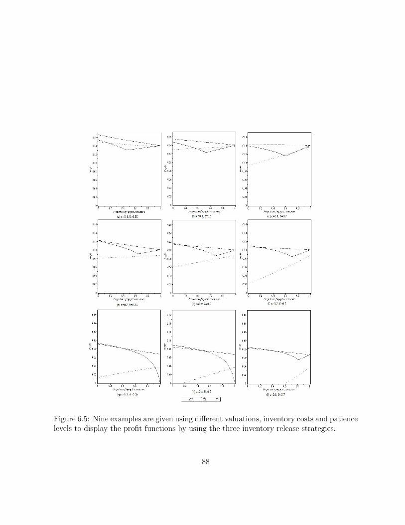
Figure 6.5: Nine examples are given using different valuations, inventory costs and patiencelevels to display the profit functions by using the three inventory release strategies.
88

Chapter 7
Summary and Managerial Insights
Our work sheds some insight into pricing strategies under uncertain demand in the presence
of strategic consumers. In our model, a monopoly retailer sells a single kind of product
over a two-period selling horizon faced with uncertain demand. We analyze three inventory
release strategies and the corresponding pricing policies with limited capacity level. We
perform the analysis by normalizing the high demand level to 1 and the low demand level
to 12, each occurring with equal probability.
With a low inventory level, a Clearance Sale strategy, the case where all leftover in-
ventory is released to the market in the third stage, is employed, and the uncertainty with
respect to the consumer quantity may cause the retailer to charge higher price under high
demand and a lower price under low demand in period 2. The same holds true if Inter-
mediate Supply strategy is adopted for an intermediate inventory level. Dynamic Pricing
strategy shall be used if the inventory level is high.
89

Based on the results from analyzing these three inventory release strategies, we prove
that the existence of strategic consumers may actually benefit the retailer. A retailer
may also obtain extra profit if strategic consumers have high levels of patience employing
Intermediate Supply strategy. This combination of findings provides some support for the
conceptual premise that strategic consumers’ behavior may actually benefit the retailer if
the retailer can clearly understand it.
Consider the Clearance Sales and Intermediate Supply strategies, the retailer’s profit
function is strictly concave in the inventory quantity stocked, which guarantee an optimal
inventory decision. Interestingly, the inventory level decreases as more myopic consumers
exist in the market in Clearance Sales strategy, which implies that as myopic consumers are
more numerous in the market, the retailer chooses a lower capacity. As strategic consumers
are more patient in cases of basic Skim Both and Skim Myopic, the retailer’s profit strictly
decreases. However, as strategic consumers are more patient, the retailer gets less profit
under Skim Both cases and the retailer’s profit is irrelevant with patience level under Skim
Myopic cases when all inventory units are sold in period 1 under high demand level or
some leftovers exist after the selling season. The retailer isolates myopic consumers from
the strategic consumers in Skim Myopic so that he can price differently for those two
groups. The retailer ignores strategic consumers’ patience level when he makes the pricing
decisions.
We find that a retailer is mostly better off employing an Intermediate Supply strategy
if he can make decisions about both inventory level and an inventory release strategy. A
few examples also show that the Clearance Sale strategy emerges as the optimal inventory
release strategy when inventory costs and/or consumers’ patience levels are high. This
90

thesis has given an account of and the reasons for the widespread use of Clearance Sale
strategy as the inventory release strategy. Our study also confirms previous findings and
contributes additional evidence that suggests retailers should employ Intermediate Supply
strategy as the inventory release policy under uncertain demand when inventory costs
and/or consumers’ patience levels are low.
This thesis can stimulate further research. For examples, we have assumed that con-
sumers are risk neutral. However, this assumption can be relaxed and explored the corre-
sponding effects when consumers are, for instance, risk averse. The risk averse consumers
are reluctant to purchase in period 2 with an uncertain payoff rather than purchasing in
period 1 with a more certain, but possibly lower, expected payoff. If strategic consumers
are risk averse, less strategic consumers wait and purchase in the second period. Retailers
may charge a higher price in period 1 to increase their profits. As myopic consumers are
more numerous in the market, the retailer’s profit may increase as well.
Another direction related to the inventory release strategy we have studied. As numer-
ical results indicate, a retailer is better off employing an Intermediate Supply strategy if
he can make decisions about both inventory level and an inventory release strategy when
inventory costs and/or consumers’ patience levels are low. Future research question can
focus the Intermediate Supply strategy’s attributes since it may be adopted widely under
uncertain demand markets. Since Intermediate Supply strategy is derived from Clearance
Sales strategy and Dynamic Pricing strategy, it is reasonable to assume that they share
some attributes. A good example in case is that the retailer’s profit may decrease as the
consumer’s patience level increase.
91

Appendices
Definitions
Inputs:
v: consumer’s valuation, which is assumed to be uniformly distributed between 0 and
1.
δ: patience level of strategic consumers.
α: fraction of myopic consumers in the market; 1 − α is the fraction of strategic con-
sumers in the market.
c: inventory cost per unit.
p: probability of high level of demand.
Ni: number of consumers arriving at the beginning of the selling season under state i,
i ∈ {H,L}, where H stand for High and L stands for Low.
We have Ni =
NH w.p. p
NL w.p. 1− p
92

Dit (≤ K): the realized demand under state i, i ∈ {H,L}, in period t, t ∈ {1, 2}.
Decisions:
K: inventory level.
R1: posted selling price in period 1.
Ri2: selling price in period 2 under state i, i ∈ {H,L}.
Pricing Policies:
(1) Skim Both (SB): price to skim high-valuation consumers of both types in the first
period, implying V < 1.
(2) Skim Myopic (SM): price to skim only high-valuation myopic consumers in the first
period. That is, none of the strategic consumers purchases in the first period; they all wait
for the second period; i.e. V = 1.
Inventory Release Strategies:
(1) Clearance Sale strategy (CS): After the first-period demand is realized, all leftover
inventory is released to the market and the market determines the price.
(2) Dynamic Pricing strategy (DP): After the first-period demand is realized, the left-
over inventory is released to maximize profit ignoring the capacity constraints.
(3) Intermediate Supply strategy (IS): After the first-period demand is realized, the
leftover inventory is released to maximize the profit under low demand and all left over
inventory is depleted under high demand, after the first-period demand is realized.
93
Bibliography
Aviv, Y. and A. Pazgal. (2008). Optimal pricing of seasonal products in the presence
of forwardlooking consumers. Manufacturing and Service Operations Management, 10(3):
339-359.
Besanko, D., W. L. Winston. (1990). Optimal price skimming by a monopolist facing
rational consumers. Management Science, 36(5) 555-567.
Bitran, G. and Caldentey, R. (2003). An overview of pricing models for profit manage-
ment. Manufacturing and Service Operations Management, 5(3):203–229.
Bitran, S. V. Mondschein. (1997). Periodic pricing of seasonal products in retailing.
Management Science, 43 64–79.
Bremaud, P. (1980). Point Processes and Queues, Martingale Dynamic Clearance Sales.
Springer-Verlag, New York.
Cachon, G. P. and R. Swinney. 2009. Purchasing, pricing, and quick response in the
presence of strategic consumers. Management Science, 55(3): 497–511.
Chan, L. M. A., Shen, Z. J. M., Simchi-Levi, D., and Swann, J. L. (2004). Coordination
of pricing and inventory decisions: A survey and classification. In Simchi-Levi, D., Wu,
S. D., and Shen, Z. J. M., editors, Handbook of Quantitative Supply Chain Analysis:
Modeling in the E-Business Era, pages 335–392. Kluwer Academic Publishers.
Elmaghraby, W., A. Gulcu, P. Keskinocak. (2002). Optimal markdown mechanisms
in the presence of rational customers with multiunit demands. Manufacturing and Service
Operations Management, 10(1): 126-148.
Elmaghraby, W. and Keskinocak, P. (2003). Dynamic pricing in the presence of inven-
tory considerations: Research overview, current practices, and future directions. Manage-
ment Science, 49(10):1287–1309.
94

Fei, S., and Xie, J. (2001). Probabilistic Goods: A creative way of selling products and
services. Marketing science. Vol. 27, No. 4, July-August 2008, pp. 674-690
Feng, Y., G. Gallego. (1995). Optimal starting times for end-of-season sales and
optimal stopping times for promotional fares. Management Science, 41 1371–1391.
Feng, Y., and G. Gallego. (2000). Perishable asset revenue management with Marko-
vian time dependent demand intensities. Management Science, 46 (7): 941-956.
Gallego, G., G. J. van Ryzin. (1994). Optimal dynamic pricing of inventories with
stochastic demand over finite horizon. Management Science, 40 999–1020.
Gupta, D., A. V. Hill, T. Bouzdine-Chameeva. 2006. A pricing model for clearing end-
of-season retail inventory. European Journal of Operational Research, 170(2) 518–540.
Lazear, E. P. (1986). Retail pricing and clearance sales. American Economic Review,
76(1): 14-32.
Levin, Y., J. McGill, J., and M. Nediak. (2009). Optimal dynamic pricing of per-
ishable items by a monopolist facing strategic consumers. Production and Operations
Management, 19(1): 40-60.
Liu, Q., van Ryzin, G. (2008). Strategic capacity rationing to induce early purchases.
Management Science, 54:1115–1131.
Mantrala, M. K., S. Rao. 2001. A decision-support system that helps retailers decide
order quantities and markdowns for fashion goods. Interfaces 31(3) S146–S165.
Shen, Z.-J. M. and Su, X. (2007). Customer behavior modeling in profit management
and auctions: A review and new research opportunities. Production and Operations Man-
agement, 16(6):713–728.
Smith, S., D. Achabal. (1998). Clearance pricing and inventory policies for retail
chains. Management Sci. 44 285–300.
Stokey, N. L. 1979. Intertemporal price discrimination. Quarterly Journal of Economi-
Clearance Sales 93(3) 355-371.
95

Su, X. (2007). Intertemporal pricing with strategic customer behavior. Management
Science, 53(5): 726-741.
Swinney, R. (2010). Selling to strategic consumers when product value is uncertain:
The value of matching supply and demand. Forthcoming in Management Science.
Talluri, K. T. and van Ryzin, G. J. (2004). The Theory and Practice of Profit Manage-
ment, volume 68 of International Series in Operations Research and Management Science.
Springer.
Xie, J. and Shugan, S. M. (2001). Electronic tickets, smart cards, and online prepay-
ments: When and how to advance sell. Marketing Science, 20 (3), 219-243.
Zhang, D. and W. L. Cooper. (2008). Managing clearance sales in the presence of
strategic customers. Production and Operations Management, 17(4): 416–431.
On the threshold purchasing behavior of customers facing dynamically priced perishable
products. Working paper, University of Washington, Seattle.
Zhou, Y. P., M. Fan, M. Cho. (2009). Strategic Consumer Response to Dynamic
Pricing of Perishable Products. Chapter 17 of “Consumer-Driven Demand and Opera-
tions Management Models: A Systematic Study of Information-Technology-Enabled Sales
Mechanisms”, Netessine and Tang (Eds.), Springer.
1.3
96