Dynamic Power Management in Embedded Systems

Rajesh Gupta, UC San Diego

http://mesl.ucsd.edu

February 2007

Outline

The case for energy and power efficiencyWhere does power go?What is new?

What is dynamic power management?DPM versus DSS

Managing Power Across Multiple LayersApplication, System Software, Architecture, HW

Summary

No Moore’s Law For Batteries

2-3% growth per year in battery capacity

Source: J. Rabaey, UC Berkeley

Not that we would want it either…Power (Energy) Density Source of Estimates

Batteries (Zinc-Air) 1050 -1560 mWh/cm3 (1.4 V) Published data from manufacturersBatteries(Lithium ion) 300 mWh/cm3 (3 - 4 V) Published data from manufacturers

Solar (Outdoors)15 mW/cm2 - direct sun

0.15mW/cm2 - cloudy day. Published data and testing.

Solar (Indoor).006 mW/cm2 - my desk

0.57 mW/cm2 - 12 in. under a 60W bulb TestingVibrations 0.001 - 0.1 mW/cm3 Simulations and Testing

Acoustic Noise3E-6 mW/cm2 at 75 Db sound level

9.6E-4 mW/cm2 at 100 Db sound level Direct Calculations from Acoustic TheoryPassive Human

Powered 1.8 mW (Shoe inserts >> 1 cm2) Published Study.

Thermal Conversion 0.0018 mW - 10 deg. C gradient Published Study.

Nuclear Reaction80 mW/cm3

1E6 mWh/cm3 Published Data.

Fuel Cells300 - 500 mW/cm3

~4000 mWh/cm3 Published Data.

Must reduce power, energy consumption.

Processor MHz Year SPECint-95 WattsP54VRT (Mobile) 150 1996 4.6 3.8P55VRT (Mobile MMX) 233 1997 7.1 3.9PowerPC 603e 300 1997 7.4 3.5PowerPC 604e 350 1997 14.6 8PowerPC 740 (G3) 300 1998 12.2 3.4PowerPC 750 (G3) 300 1998 14 3.4Mobile Celeron 333 1999 13.1 8.6

Low Power Has Been A Design Focus

Speed power efficiency has indeed gone up10x / 2.5 years for μPs and DSPs in 1990s

between 100 mW/MIP to 1 mW/MIP since 1990IC processes have provided 10x / 8 years since 1965rest from power conscious IC design in recent years

Another 20X is possible.

Source: ISI/USC, DARPA PACC Program

Unfortunately, that is not enough

There is a bottom line to energy efficiency…Computation cost (2004 projected): 60 pJ/op Minimum thermal energy for communications:

20 nJ/bit @ 1.5 GHz for 100 m2 nJ/bit @ 1.5 GHz for 10 m

… but not to the need for energy (or power).

The New Age Computing & Comm.

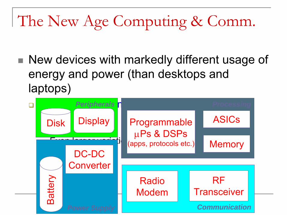
New devices with markedly different usage of energy and power (than desktops and laptops)

Much wider dynamic range of power demand6-10X variation in power from sleep to various active modes; Even larger variation in radio power, TX/RX ratio

Power Supply

Bat

tery

DC-DCConverter

Communication

RadioModem

RFTransceiver

Processing

ProgrammableμPs & DSPs

(apps, protocols etc.) Memory

ASICs

Peripherals

Disk Display

“System Design”

for Low Power

Energy efficiency (has to) cut across all system layerscircuit, logic, software, protocols, algorithms, user interface,power supply... Node versus network

Trade-off between energy consumption & QoSoptimize energy metric while meeting “quality” constraint

When all low power tricks have been done, “duty cycling” remains the only available variable to reduce energy consumption

Must capture the “application intent”.

Shutdown for Energy Saving

Use low duty cycle of many subsystems:

Large difference between “on” & “off” power

Blocked“Off”

Active“On”

Tblock Tactive ideal improvement = 1 + Tblock/Tactive

Example: SA-1100 CPU

RUNIDLE

CPU stopped when not in useMonitoring for interrupts

SLEEPShutdown on-chip activity

RUN

IDLE SLEEP

400 mW

50 mW 0.16 mW

90 μs

10 μs 10 μs 90 μs

160 ms

Example: Fujitsu MHF 2043 AT

Working: 2.2 W (spinning + I/O)

Idle: 0.95 W (spinning)

Sleep: 0.13 W (stop spinning)

spin up 4.4 J, 1.6 s

shutdown 0.36 J, 0.67 s

read/write

I/O done

A Generic Power-managed System

Lots of prior and ongoing activity in defining the interface between power-manageable components (chips, disk driver, display driver, radios, etc.) and the power manager (PM)Components (or service providers) have internal states

Abstracted as power state machinepower and service annotation on states; power and delay annotation on edges

PM Policy: uses insight into how and when to invoke PM

PowerManager

ServiceRequestor

ServiceProvider Queue

observationobservation

command (on, off)

request

E.G.: Dynamic Speed Scaling: V/f Generic system architecture

many examples in hardware and software

Variable Power-Speed

SystemFIFO Input Buffer

Workload Filter

Power-SpeedControl Knob

Controlling Power/Energy Consumption

DPM “shutdown” through choice of right system & device states

Multiple sleep states

DSS“slowdown” through choice of right system & device states

Multiple active states

DPM + DSSChoice between amount of slowdown and shutdownHowever, the problem changes “qualitatively”.

Slowdown Preferred Over Shutdown

Example: 50ms task with 100ms deadline50ms computation, 50ms idle/stopped timeHalf speed: 100ms computation, 0ms idle

¼ energy than the full speed case if voltage scales

Use voltage to control the operating point on the power vs. speed curve

i.e., power and clock frequency are functions of voltage

Because of higher savings in slowdown often shutdown becomes a “secondary” strategy

First slow down and then look for ways to shutdown.

Slowdown loosing its effectiveness..

Radio’s Need Duty-cycling Too

The RF power dominates over the electronic power associated withtransmit or receive processing, except for short distances (5-10 m).Voltage scaling and other low power logic techniques do not affect RF power consumption

packet TransmitProcessing

TransmitAmplifier d

packetReceive

Processing

50 nJ/bit 100 pJ/bit/m

Source: Heinzelman ISLPED’00; Wang ISLPED’01

18

Power Management in Communication Power Management in Communication SubsystemsSubsystems

Computation Subsystem

e.g. Dynamic Voltage/Freq.

Scaling

Communication Subsystem

Modulation

coding

Power-aware Task Scheduling

OS/Middleware/Application

Power-aware Packet Scheduling

Power Savings Mechanisms

A

Dynamic Power Management (DPM) When a device is idle, it can transition to low-power “sleep” states.Current trend is to design devices with multiple sleep states and provide device driver hooks to change these states under OS control.

B

Dynamic Voltage Scaling (DSS, or DVS) A device can be run at different speeds at different power levelsExecution of jobs can be slowed down to save power as long as all jobs are completed by their deadline.

C

Application level “knobs”quality and performance measures, application tolerances

A

B

C

A. Dynamic Power Management

When a device becomes idle, it can transition to lower power usage state.A fixed amount of additional time and energy are required to transition back to active state when a new request for service arrives.What is the best time threshold to transition to the sleep state?

Too soon: pay start-up cost too frequently.Too late: spend too much time in the high-power state

Generally, transition to sleep state when the cost of being in active state is at least the cost of ‘waking up’.

A

Our Work In This Context

We have developed quantitative bounds on the quality of DPM algorithms based on Competitive Analysis [TCAD 01]

provides a basis for DPM strategy comparison

Developed DPM strategies for devices with both multiple active and multiple sleep states [TCAD 02]

Design and analyze algorithms for systems that allow both DPM and DVS [SODA 03, TECS02]

Important conclusionsNot all power states are useful in a given DPM strategyDPM generally useful for improving quality measures.A

Competitive AnalysisDeterministic algorithm (ski rental)

Transition to sleep state when the cost of being in active state is at least the cost of ‘waking up’.

Normalize cost of transitioning from sleep to active state to 1.Power consumption rate of active state is α.

This algorithm is 2-competitive.2 is the best possible competitive ratio for any deterministic algorithm.

Probabilistic algorithmIdle period length generated by known distribution with density function p(t).Choose threshold T to minimize cost:

For any distribution p(t), the expected cost of the above algorithm is within e/(e-1) of the optimal cost. Furthermore, there is a distribution for which no algorithm can be better than e/(e-1) times optimal.

∫∫∞

+[+T

T

TdttpTdttpt )(]1)(minarg

0

αα

A

Multi-state DPM Case

Let there be k+1 statesLet State k be the shut-down state and 0 be the active stateLet αi be the energy dissipation rate at state iLet βi be the total energy dissipated to move back to State 0States are ordered such that αi+1 ≤ αi

αk = 0 and β0 = 0 (without loss of generality).Power down energy cost can be incorporated in the power up cost for analysis (if additive).

Now formulate an optimization problem to determine the state transition thresholds.

A

Energy

Time

State 4

State1 State2 State3

t1 t2 t3

ii TimeEnergy βα += )(For each state i, plot:

Lower Envelope Idea

LEA can be deterministic or probabilistic

PLEA is e/(e-1) competitive.∫

∫∞

−

−−

+−+[+

+=

Tiii

T

iiT

i

dttpTtT

dttptT

)(])(

)(][minarg

1

011

βαα

βα

A

Model Checking

•

Model the system as a two player game between DPM algorithm and a non-

deterministic adversary–

Adversary can generate the worst-case input for the algorithm.

•

Use model checking to automatically verify whether a specific algorithm achieves a given competitive ratio.

[Shukla, Gupta 01]

0s02.4Active/Busy

40ms0.560.9Idle

1.5s1.5750.2Stand-by

5s4.750Sleep

Transition Time to Active

Start-up Energy (Joules)

Power Consumption

State

Trace data with arrival times of disk accesses from Auspex

file server archive.

Experimental Study: IBM Mobile Hard Drive

A

IBM Mobile Hard Drive

0

0.5

1

1.5

2

2.5

0 500 1000 1500 2000 2500

Latency

Com

petit

ive

Rat

io w

rt E

nerg

y U

sage

OptimalLEAPLEALAST:PLAST:NPTREE:PEXP:PEXP:NP

Comparison of Energy Dissipation between the Deterministic and Probability Based Strategies

0

1

2

3

4

5

6

Trace1

Trace3

Trace5

Trace7

Trace9

Trace1

1Trac

e13

Trace1

5

Traces

Joules

Deterministic online

Probability BasedonlineOptimal Offline

A

B. Dynamic Voltage ScalingDevice which can run at any speed s.

Power consumed if running in state s is given by convex function P(s).

Jobs arrive through time. Job j has:Arrival time: aj

Deadline: bj

Work required: Rj

Schedule S = (s, job)s(t) is the speed of the device at time t.job(t) is which job is executed at time t.

B

Dynamic Voltage Scaling (Dynamic Voltage Scaling -

No Sleep: DVS-NS)

Schedule S is feasible for set of jobs J if for every j in J:

Cost of Schedule S is:

∫ =j

j

b

ajRdtjtjobts )),(()( δ

∫=1

0

))(()(cost

t

dttsPSt

B

DVS with Sleep State (DVS-S)

Schedule S = ( s, job, h ):h(t) = sleep or onIf h(t) = sleep, then s(t) = 0.

Power is a function of speed and state:P(s, state) = P(s) if state = on.P(s, state) = 0 if state = sleep.

P(0) = α is power required to keep device active with no tasks running.Let k be the number of times the device transitions from sleep state to the on stateCost of a schedule S is: ∫+=

1

0

))(),(()(cost

t

dtthtsPkSt

B

Critical SpeedIf the cost to transition from sleep state to the on state were 0, the optimal speed for all jobs would be the s that minimizes (Rj/s) P(s)

This is the s that satisfies P(s) = s P’(s).Call this Scrit, the critical speed for α.

If we compress the execution of a task by x, we expend additional energy because we execute the job faster we save α x. Scrit is the point at which it is no longer beneficial to compress the execution of a task.

Our approachDecide on Active/Idle intervals (determined by critical speed)Decide on Sleep/On intervals (determined by the cost of staying on)

B

C. Enable Application “Knobs”

Knowing an application’s intent one can do a lot of power saving tricks at all levels: architecture, compiler, OS, middleware

Conversely, if the awareness for power/energy is seeped into all these levels, one can reduce power significantly

Together they can create a new contract in the computing system!

Since power is important in radios, things with radios move (or they monitor things that move), location awareness is even more phenomenal for power reduction.

C

Outline: Bringing energy awareness in application, OS and Middleware

Application

OS

Middleware

A

B

C

What does is mean to be ‘aware’?

That the application and the services knowabout energy, power

File system, memory management, process schedulingMake each of them energy aware

How does one make software to be “aware”? Use “reflectivity” in software to build adaptive softwareAbility to reason about and act upon itself (OS, MW)

Reflection and Introspection: A HW Guy’s Way of Looking At It

Component:A unit of re-use with an interface and an implementation

Meta-information:Information about the structure and characteristics of an object

Reification:A data structure to capture the meta-information about the structure and the properties of the program

Reflection:An architectural technique to allow a component to provide the meta- information to himself

Introspection:The capability to query and modify the reified structures by a component itself or by the environment

5 portsadder

Building HW Components W/ Meta-data1.

Start with SystemC

descriptions of IP blocks

Multi-level (RTL, TL) descriptions

2.

Capture meta information of these IP into XML

Mostly structural information for now.

3.

Generate library of ‘XMLized’

IP blocks

Schema to match datatype and protocol type information across IP blocks Create DOM model and constraints for the library

4.

Develop methods for IP selection, composition, verification, synthesis

Automated methods for IP instantiation, interface generation

IP Selection through an Introspective Composer ● IP matching and connection○ Insertion of bridges ○ Validation of functionality○ Create an executable specification

Applying Reflection: performance, energyUse Meta data to represent resource demands, dynamic behavior of the program carrying it.

Resources: Memory (R/W, Cache), Processor (IPC)Enables energy-performance tuning by exploring resource demand variations throughout programs’ execution

Example: Profile of application over memory banksVary frequency of processor based on IPC demand

A

Example: Rambus DRAM (RDRAM)High bandwidth (>1.5 GB/sec)Each RDRAM module can be activated/deactivated independentlyRead/write can occur only in the active modeThree low-power operating modes:

Standby, Nap, Power-Down

A

Active

3.75 nJ

Active

3.75 nJ

Napping

0.32nJ

30 cycles

Napping

0.32nJ

30 cycles

Power-Down

0.005 nJ

9000 cycles

Power-Down

0.005 nJ

9000 cycles

0.83 nJ

2 cycles

Standby

0.83 nJ

2 cycles

Standby

CPU +CachesCPU +

Caches

BankBank

0

N-1

BankBank

3N

4N-1

BankBank

N

2N-1

BankBank

2N

3N-1

BankBank

0

N-1

BankBank

0

N-1

BankBank

3N

4N-1

BankBank

3N

4N-1

BankBank

N

2N-1

BankBank

2N

3N-1

BankBank

2N

3N-1

Approach1.

Characterize application offlineDivide an application into phases of execution

A group of program intervals executing similar code

Each phase has similar demand on resourcesSimilar code, similar resource demands (memory, IPC)

2.

Annotate source codePhase signatures

3.

Enable OS (and hardware) to recognize signature

Smart hardware and/or online learning techniques4.

Dynamically tune the power manager As application moves from one phase to another.A

1 Understanding application behaviorDivide an application into phasesof execution

A group of program intervals executing similar code

Each phase has similar demand on resources

Similar code, similar resource demands

Demand for resources varies during the execution of application

As it moves from one phase to another.

Phases identified using BBV or LBV

Keep track of loop branches

A

2 Offline analysis of applicationA data structure with the summary of the information of interest for each phase is attached to the program

Fixed location for the program metadataOS support to access metadata.

Also a signature of each phase is attached to the program.

No. of times the loops of the program are executed in the particular phase

A

Dynamic Program Execution

………

… …

…

… +

+

+

Resource demand meta data

Phasesignatures

Programs meta data

…

…

…

Dynamic Program Execution

………………

…… ……

……

…… +

+

+

Resource demand meta data

Phasesignatures

Programs meta data

……

……

……

3 Runtime AnalysisChallenge:

Detect in which phase the program is running Learning, signature construction, partial matches

Match the signature created offline with a online signature using Manhattan distance.

If distance < threshold a match is found. Threshold tells how similar two intervals of execution are.

The same technique used for splitting the program in phases offline is applied online but using partial signatures for matching with the offline computed signatures.

A

4 Matching signature at runtime

Use performance counters:Can be programmed to generate an interrupt on specified counts

ISR provides matching with the meta data and mode changesEvery S*10,000 loop branches try a matchPhase matching can also be done in hardware

Notify power manager to trigger proper action

A

Adaptation for Memory Behavior

Number of engineering optimizationsFrequency of adaptationGranularity of analysis (phase granularity)Tradeoff against cost of adaptation.

Results – Normalized to NAP

Average among bzip, mpeg, ghostscript

and ADPCM

A

Results - overheadsApprox. 350K instructions for every 10,000 loop branch instructions Number of instructions executed by the match algorithm at every 10,000 loop branches to match a partial signature (500 instructions per phase)

# of phases # instructions overhead

5 2,580 0.7%

10 4,500 1%

20 8,280 2%

30 12,060 3%

Size overhead. 4 bytes per inter arrival estimate per bank / phase. 4 x 16 x 10 = 640 bytes assuming 16 banks and 10 phases. The signatures take1280 bytes for 10 phases. Total of 2KB of meta data

A

“Hardware”

View

Sensors RadioCPU

Energy-aware RTOS, Protocols, & Middleware

PA-APIs for Communication, Computation, & Sensing

Dynamic Voltage &

Freq. Scaling

Scalable Sensor

Processing

Freq., Power, Modulation, & Code Scaling

Coordinated Power Management

Hardware

Sensors RadioCPU

Energy-aware RTOS, Protocols, & Middleware

PA-APIs for Communication, Computation, & Sensing

Dynamic Voltage &

Freq. Scaling

Scalable Sensor

Processing

Freq., Power, Modulation, & Code Scaling

Coordinated Power Management

Hardware

Going Forward: Multiple Radios Are Common

HP h6300: GSM/GPRS, BT, 802.11 Moto

CN620: BT, 802.11, GSM

802.11x, BT, GSM

These radios typically function as isolated air interfaces to isolated networks.

Collaborating Radios Can

Improve PerformanceAggregate connectivity

Improve ReliabilityRadios as backup interfaces

Improve SecurityMultiple/Side-Channel Authentication

Improve Efficiency (Spectral, Energy)Dynamically match radios to traffic, rangeUse radios to page another, duty cycle other radios

►

Collaborating radios have a great potential for system-wide improvement●

Energy, mobility management, capacity enhancement, channel failure recovery, networking, security, ….

●

We focus on energy.

Typical power distribution

CPUSDRAMBluetoothWi-FiOther

CPU:47 mW

WiFi: 786 mW

SDRAM:86 mW

Bluetooth112 mWOther:

251 mW

Power breakdown for a fully connected mobile device in idle mode, with LCD screen and backlight turned off.

Depending on the usage model, the power consumption of emerging mobile devices can be easily dominated by the wireless interfaces!

Common Radio Standards

050

100150200250300350400450

Zigbee BT 802.11

Idle

Pow

er (m

W)

0

50

100

150

200

250

Ener

gy/B

it (n

J/bi

t)

0.25Mbps 1.1Mbps 11Mbps

Higher throughput radios have a lower energy/bit value … have a higher idle power consumption

And they have different ranges.

Consider: BT and WiFi

Objective: Always-on low-power operation with high peak bandwidth and overall energy efficiencyTwo possibilities:1.

Use BT to page WiFi

as needed2.

Build a switching hierarchy for energy efficient operationEffectively expand the power states available at the system levelSwitching policies are key to a good implementation.

WiFi

Active WiFi

Active

WiFi

PSM

WiFi

ActiveBT

Active

WiFi

ActiveBT

Sniff

Bluetooth Wi-Fi

264 mW 990 mW81 mW5.8 mW

C 1

C 3

C 2

C 4

802.11 Data

BT Data

802.11 Interface

Bluetooth Interface

1

3 4

5

2

7

6

802.11b BT

DUAL AP

C1, C2, C3, C4 − Mobile Clients

Range of BT Paging Channel

Scenario : An application on C1

wants to communicate with C3

1.

C1 turns its 802.11 radio ON2.

C1 starts communication, sends data to AP through 802.11

3.

AP matches C3’s destination IP with its BT address

4.

AP sends WAKE-UP page to C3 via it’s BT interface, C3 turns on it’s 802.11 radio on receiving the WAKE-UP page

5.

When C1 finishes sending data it switches OFF its 802.11 radio

6.

If all connections to and from C3 are closed, AP sends SLEEP page

7.

On receiving SLEEP page C3 turns

OFF its 802.11 radio

1. BT as a paging radio

Simple paging (with range compensation)

Implemented iPAQs (3870), familiar linux and CISCO PCM-350, built-in BTMeasured power and latency on FTP and SSH sessions

Average Power Consumption

0

0.5

1

1.5

2

2.5

3

CAM PSP SS1 SS2

Aver

age

Pow

er (W

atts

)

Total Power 802.11b Card only

40% better Vs CAM8% better Vs PSP 48% better Vs CAM

23% better Vs PSP

Normalised Energy -- Scripts

0

0.2

0.4

0.6

0.8

1

1.2

CAM PSP PowerManagement

SS1

PowerManagement

SS2

Various Configurations

Nor

mal

ised

Ene

rgy

Script - FTP1Script - SSH1

830 1394

680

955640

948 582885

Power Savings for 802.11 card only vs PSP : 41% (SS1) to 95% (SS2) Throughput - Same as Awake Mode (CAM) , maximum throughputLatency - Setup latency, amortized across session

2. CoolSpots: Radio Hierarchy

Wi-Fi HotSpot

CoolSpots Network Architecture

Infrastructure Computers

CoolSpot

Access Point

BT WiFi

BT WiFi Mobile Device

IP address on

Backbone Subnet

Low-power Bluetooth link

(always maintained, when possible)

1

Mobile device monitors channel and implements switching policy

2

WiFi link is dynamically activated based on switching determination

3

Access point changes routing table on “switch”

message from mobile device

4

Switching is transparent: applications always use the IP address of the local subnet.

5

Backbone Network

Switching Policies

Three main components contribute to the behavior of a multi-radio system

Position: Where you areNeed to address the difference in range between Bluetooth and WiFi

Benchmarks: What you are doingApplication traffic patterns greatly affect underlying policies

Policies: When to switch interfacesA non-intrusive way to tell which interface to use

Where: Position

Different radio ranges affect the switching decisionHowever, optimal switching point will depend on exact operating conditions, not just rangeExperiments and (effective) policies will measure and take into account a variety of operating conditions

Position 1

Position 3

Bluetooth channel capacity depends on range, so the further away you are, the sooner you need to switch…

Base Station

In some situations, Bluetooth will not be functional and WiFi will be the only alternative

Position 2

What: Benchmarks

Baseline: target underlying strengths of wireless technologies

• Idle: connected, but no data transfer

• Transfer: bulk TCP data transfer

WWW: realistic combination of idle and data transfer conditions• Idle: “think time”• Small transfer: basic web-pages• Bulk transfer: documents or media

Video: range of streaming

bit-rates varying video quality• 128k, 250k, 384k datarates• Streaming data, instant start

What: Benchmarks

Benchmark Time over WiFI

DataTransmitted

Average Bandwidth(Data Size / Time)

Data Pattern

idle 60s 0.0 MB 0 kbps Nonetransfer-1 13s 6.6 MB 4482 kbps Bulk transfertransfer-2 27s 13.3 MB 4519 kbps Bulk transferwww-intel 176s 21.6 MB 1022 kbps Intermittent datawww-gallery 150s 2.9 MB 158 kbps Intermittent datavideo150k 150s 3.1 MB 172 kbps Real time streaming

videovideo250k 150s 7.3 MB 402 kbps Real time streaming

videovideo384k 150s 8.5 MB 464 kbps Real time streaming

video

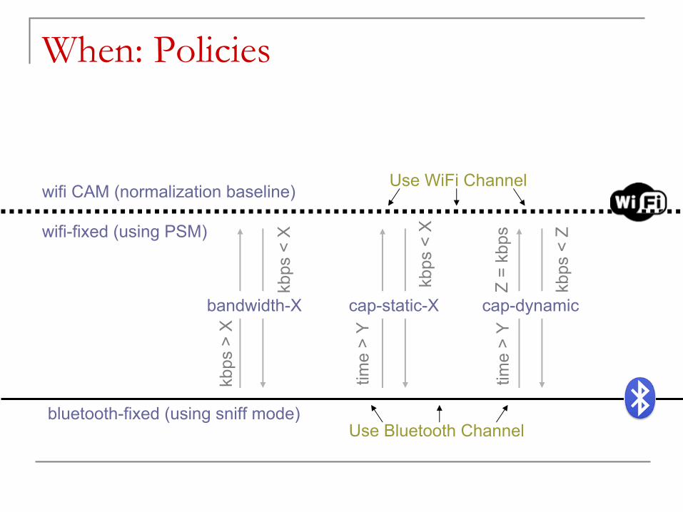
When: Policies

bluetooth-fixed (using sniff mode)

wifi CAM (normalization baseline)

wifi-fixed (using PSM)

bandwidth-X cap-static-X cap-dynamic

kbps

> X

kbps

< X

kbps

< X

time

> Y

time

> Y

kbps

< Z

Z =

kbps

Use WiFi Channel

Use Bluetooth Channel

Experimental Setup

Characterize power for WiFi & BTMultiple Policies Different locations Suite of benchmark applications

Stargate research platform400Mhz processor, 64MB RAM, LinuxAllows detailed power measurement

Tested using “today’s”

wireless:WiFi is NetGear

MA701 CF cardBluetooth is a CSR BlueCore3 module

Use the geometric mean to combine benchmarks into an aggregate result

Moved devices around on a cart to vary channel characteristics

Test Machine

(TM)

Base Station (BS)

RM

Mobile Device (MD)SP

Data Acquisition

(DA)

ETH

BT

WiFi

mW

Distance adjustment

ETH = Wired Ethernet

mW = Power MeasurementsBT = Bluetooth WiFi = WiFi

WirelessRM = Route Management

SP = Switching Policy

Benchmark suite

Switching Example: MPEG4 streaming

Switch : Wi-Fi -> BT

Bluetooth

Wi-Fi- Simple bandwidth policy

-

Switch from WiFi

to BT when application has buffered enough data

Switching is transparent to unmodified applications!

Results (Intermediate Location)

0%

20%

40%

60%

80%

100%

wifi-CAM

wifi-fixed

bandwidth-30

cap-static-30

cap-dynamic

blue-fixed

Switching Policy (Fixed Range, Aggregate Benchmark)

Nor

mal

ized

Ene

rgy

0%

50%

100%

150%

200%

250%

Nor

mal

ized

Tim

e

WiFi EnergyBluetooth EnergyTime

• blue-fixed does well in terms of energy but at the cost of increased latency

• cap-dynamic does well in terms of both energy and increased latency

Impact of Range/Distance

0%

10%

20%

30%

40%

50%

60%

70%

80%

wifi-fixed

bandwdith-0

bandwidth-30

bandwidth-50

cap-static-0

cap-static-30

cap-static-50

cap-dynamicblue-fixed

Switching Policy

Ener

gy

Location 1

Location 2

Location 3Bandw idth Policies

Cap-Static Policies

Missing data indicates failure of at least one application, and therefore an ineffective policy!

L1: 3mL2: 7mL3: 11m NLOS

Results across various benchmarks

0%

20%

40%

60%

80%

100%

120%

140%

Idle transfer-1 transfer-2 www-intel www-gallery

video128k video250k video384k

Benchmark

Ener

gy

wifi-fixed

bandwidth-30

cap-dynamic

blue-fixed

wifi-fixed consumes lowest energy for data transfer, any bluetooth policy for idle

Overall, cap-dynamic does well taking into account energy and latency

Video benchmarks really highlight problems with wifi-fixed and bandwidth-x

Cap-Dynamic Switching Policy

Switch up based on measured channel capacity(ping time > Y): 40ms-800ms, estimates channel conditions

Remember last seen Bluetooth bandwidth (Z=kbps)

Switch down based on remembered bandwidth (kbps < Z): limited mobility

time > Y

kbps < Z

Z = kbps

Switching Policies –

Summary

“Wifi-Fixed” Policy (WiFi in Power Save Mode) Works best for as-fast-as-you-can data transfer Higher power consumption, especially idle power

“Blue-Fixed” PolicyVery low idle power consumptionIncreases total application latency, fails at longer ranges

“Bandwidth” Policy Static coded bandwidth thresholds, fails to adapt at longer rangesSwitches too soon (bandwidth-0) or switches too late (bandwidth-50)

“Capacity-Static” Policy Estimates channel capacity and uses that to switch up Fails at longer ranges due to incorrect switch-down point

“Capacity-Dynamic” Policy Dynamic policy, remembers the last seem switch-up bandwidth Performs well across all benchmarks and location configurations!

Closing Thoughts

Algorithmic approaches to power management have come a long way

Realistic models of the system, and its environmentThe challenge remains how a “good” PM is actually implemented

Going forward, a comprehensive “awareness” of energy is needed from application to distributed hw/sw infrastructureMultiple radios open up many possibilities for system-level performance and reliability increases

CoolSpots shows ~50% reduction in energy consumption over current power management in WiFi across applications, ranges

Many improvements possible that take into accountApplication behavior, Radio link quality, Network queues instead of ping latency, other scenarios (multi-user environments, p2p configurations)Network infrastructure instead of standalone CoolSpots APs