Dynamic Perspectives on Crime∗

Justin McCraryUC Berkeley, NBER

August 24, 2009

This manuscript was prepared for the Handbook of the Economics of Crime.

∗I think David Lee for collaboration on related projects and Pat Kline and Demian Pouzo for unusually helpfulcomments.

I. Introduction

Economists seeking to understand how crime might respond to policy interventions typically turn

to the model of crime due to Becker (1968). In this model, crime is viewed as a point-in-time

bet, and crime occurs when the expected utility of taking the bet is greater than the expected

utility of turning it down. Another workhorse of the economic analysis of crime is the static

time allocation model of Gronau (1977). This model has been adapted used by several authors,

including Grogger (1998), Lemieux, Fortin and Frechette (1994), and Williams and Sickles (2002).

Becker’s and Gronau’s models are static, in the sense that there is no explicit reference to the future

consequences of apprehension.

Static models of criminal labor supply lead to important insights in many contexts, but can be

awkward in contexts where dynamics are important. As one example, crimes with the greatest social

costs are serious property and violent crimes. In every modern society, these crimes are punished

by lengthy prison sentences rather than fines or instantaneous physical punishment. Thus, the

disutility associated with apprehension for the most important crimes is experienced many periods

after the utility gain associated with commitment of the crime. A second example of the importance

of dynamic considerations pertains to intertemporal substitution of criminal activity. Over the last

decade or so, a consensus has emerged in criminology that “hot spots policing”—i.e., a massive

increase in police presence within a geographically small area of a city where criminal activity has

recently been high—is a highly effective strategy for crime reduction. However, to the extent that

criminals are able to relocate activity to other time periods or other places, such strategies may

be more effective at reducing crimes in one location temporarily than in reducing crimes in the

aggregate over the medium- to long-term.

A static perspective is also limiting when it comes to the government’s problem of controlling

crime. Consider a state legislator, who is deciding whether to vote for a sentence enhancement bill,

or whether to vote for a bill to subsidize hiring of police officers on the part of localities. Assuming

modest magnitudes for deterrence elasticities, a vote for the sentence enhancement bill entails small

current costs and large future costs, whereas a vote for the policing bill entails large current costs

and medium future costs.

1

While these dynamic features of crime are interesting, they do not occupy a central place within

the current economics of crime literature. My assessment is that this is an important gap. In this

chapter, I review the literature on dynamics and crime. In light of the small size of this literature,

more attention than is usual in a review article is devoted to potentially fruitful directions for future

research.

Section II provides a brief overview of the existing small literature on dynamics and crime.

Section III emphasizes the practicality of a dynamic approach, reviewing the simple dynamic model

of crime from Lee and McCrary (2009). In Section IV, I turn my attention to the government’s

problem of minimizing the present discounted value of crime by adjusting policing and sentence

lengths appropriately, currently and in the future. As I show, this problem has many interesting

dynamic features. I am not aware of any work on this important topic. Finally, Section V concludes.

II. Literature Review

The first dynamic treatment of crime of which I am aware is Flinn (1986).1 Flinn models the

proportion of time allocated to work and crime in each period. He assumes no borrowing and no

savings and lets the probability of apprehension in period t be increasing in the amount of time

devoted to crime in period t. Upon apprehension, the individual is incarcerated for a deterministic

sentence length that can depend on prior criminal history. Wages in the legitimate market are

either fixed, or increase with experience. Flinn shows that the model is capable of matching the

age profile of crime, but does not seek to estimate or calibrate the model.

Lee and McCrary (2005, 2009) emphasize one of the most basic insights of a dynamic perspective

on deterrence: if offenders have short time horizons, then it is hard to imagine punishment acting as

an important deterrent. Empirically, most offenses occur at a time when the offender is experiencing

diminished capacity. Nationally, at the time of arrest, 65 percent of arrestees have positive urinalysis

tests for one of 5 major drugs: marijuana, cocaine, opiates, methamphetamines, or phencyclidine

(PCP). Fully 21 percent test positive for the use of more than one such drug at the time of arrest.2

1Interestingly, this paper is part of an edited volume that is extremely prominent among criminologists, butsomewhat obscure among economists.

2Estimates from the Arrestee Drug Abuse Monitoring (ADAM) program of the National Institutes of Justice.The ADAM program uses probability sampling at 35 different sites scattered throughout the U.S. Numbers reported

2

Considering the possibility of both drug and alcohol use, it seems likely that a large fraction of

offenders are prone to impulsive behavior. The mental state of the marginal offender at any given

point in time thus may well be importantly different from that of a person contemplating decisions

typically modeled in other areas of economics (how many years of schooling to obtain, lifecycle

labor supply in the legitimate labor market, marriage and fertility, and so on), and indeed may be

different than the mental state of the offender himself at other times (Strotz 1955).3

The time horizon of the offender is relevant because in every developed country around the

world, serious crimes are punished by long prison sentences, measured in years or even decades. If

the marginal offender has a short time horizon, it may be difficult to reduce his criminal propensity

by threatening additional punishment. Importantly, however, even if the marginal offender has

an extremely short time horizon, it may still be possible to reduce his criminal propensity using

enhancements to the probability of apprehension (see Section III for details).

In their empirical work, Lee and McCrary (2009) use data from Florida to measure the rate of

criminal involvement local to 18, when offenders are handled by the adult criminal justice system

instead of the more lenient juvenile system. The estimates suggest only a 2 percent decline in the

probability of offense upon transitioning to 18, when the expected period of detention, conditional

on arrest, increases by roughly 230 percent. Lee and McCrary calibrate a version of the baseline

dynamic model outlined in Section III and use the model to provide bounds for the elasticity of

crime with respect to police and with respect to an expected sentence length. These bounds are

nonparametric in the sense that they do not require a parametric restriction on the distribution of

criminal benefits and instead require that the distribution of criminal benefits has a weakly declining

density. As discussed by Viscusi (1986), for example, this assumption arises naturally from the fact

that crime is largely a transfer from victim to offender, and that criminal opportunities worth more

to an offender are likely to be taken out of circulation, or possibly “hardened” in some way, so as

to reduce the frequency of such opportunities.

Jacob, Lefgren and Moretti (2007) emphasize another important dynamic aspect of criminal

behavior: intertemporal substitution. Using data from the National Incident Based Reporting

in text reflect arrestee-weighted averages of site-specific estimates and reflect author’s calculations.3For an explicit dynamic model of offense behavior under hyperbolic discounting, see Lee and McCrary (2005).

3

System (NIBRS), these authors document that, (1) conditional on weather conditions in period t

and other period t controls, weather conditions in period t − 1 are strongly correlated with crime

in period t− 1, and that (2) using weather in period t− 1 as an excluded instrument, instrumental

variables estimates of the elasticity of the crime rate in one week with respect to the crime rate

in the past week is about -0.22 for violent crime and -0.17 for property crime. The elasticity with

respect to two weeks prior is -0.16 for violent crime and -0.14 for property crime, and the elasticity

seems to decline at longer lags.

The extent to which criminal labor supply may be substitutable, across time but also across

space, is one of the great unsolved problems of crime control. If displacement is important, then

costly attempts at saturation policing, known as “hot spots policing”, may well simply shuffle crime

from place to place or from time period to time period, with little overall impact on the present

discounted value of national crime. This is an important consideration in light of the consensus

within criminology that saturation policing is an effective tactic (Braga 2005). Perhaps prompted

by consultant criminologists, many police departments have adopted these tactics in recent years

(Heinzmann 2004, Raghavan 2005, Eiserer 2005, Higgins 2006, Hoover 2007, Katz 2009, Hunt 2009).

Displacement is not widely discussed in the literature, perhaps in part because it is so hard to

measure. The “catchment area” for the crime displaced from any hot spot is hard to identify a

priori, making it hard to design a research study to quantify the importance of displacement.

The Jacob et al. (2007) findings provide evidence that displacement is an important phenomenon,

at least within the time dimension. In light of the Lee and McCrary (2009) findings, one possible

interpretation is that it is easier to detect displacement in time than in space, because offenders

have a taste for the present and would not want to defer activity much beyond the period during it

was suppressed.4 However, Jacob et al. emphasize that their results are difficult to reconcile with

extreme scenarios in which either (1) potential offenders are unable or unwilling to save or borrow,

or (2) potential offenders have long time horizons and access to perfect capital markets. In the

first case, potential offenders solve a static problem and a period t− 1 income shock cannot affect

period t behavior. In the second case, by the permanent income hypothesis, the only role for a

4On prior grounds, displacement in space seems likely to be much more diffuse than displacement in time,particularly with respect to activities such as drug transactions.

4

period t− 1 income shock to affect period t behavior is through income effects, which the authors

note are generally thought of as small.5 Consequently, the authors prefer a hybrid scenario, in

which offenders have a short time horizon, with no saving or borrowing. Because of the short time

horizon, the scope for income effects is substantial. The authors note that they find much larger

displacement effects for property crimes such as car theft that are associated with large income

gains.

While the Lee and McCrary (2005, 2009) and Jacob et al. (2007) studies highlight that offenders

may have short time horizons, this conclusion is far from settled in the literature. A series of

important dynamic articles in the International Economic Review (IER) in 2004 each assume long

time horizons for potential offenders. These articles emphasize a variety of dynamic mechanisms

that are relevant for the study of crime.

Huang, Laing and Wang (2004) present a nuanced model with endogenous human capital accu-

mulation, heterogeneous firms, and labor market search. A major feature of the article is a clear

discussion of equilibrium. A limitation of the article, however, is the assumption that punishment is

experienced as a one-period utility loss, much as in the Becker (1968) model. This limits the ability

of the model to accomodate non-responsiveness of offenders to prison due to short time horizons.

The article makes no effort at either estimation or calibration.

Imai and Krishna (2004) emphasize the idea that engaging in crime today may have negative

consequences for completion of education and for employment and wages in the future. The ap-

proach is a partial equilibrium dynamic structural model, along the lines of that discussed in Lee

and McCrary (2009), but with a much richer specification of potentially heterogeneous preferences,

both between persons and across time. The paper explicitly estimates the dynamic model using

data from the 1958 Philadelphia Birth Cohort Study.6

The major empirical conclusion of the article is that the prospect of future reductions in labor

market employability and remuneration leads to reduced current period criminal activity (“dynamic

deterrence”). However, this substantive conclusion is intrinsically linked with the substantive con-

clusion of long time horizons: Imai and Krishna (2004) estimate an annual discount factor of 0.99.

5In addition, income effects do not predict the ”fadeout” pattern in the elasticities discussed above and thus arenot a convincing explanation for the findings.

6These data are not often used within economics, but are available from ICPSR.

5

Further, this estimate is based on the assumption that punishment lasts one period. Intuitively, if

the marginal offender has a short time horizon, then this limits the scope for dynamic deterrence,

just as it limits the scope of the effectiveness of prison as a punishment. The article does not address

the intriguing possibility that dynamic deterrence would lead a social planner to increase funding

for police, relative to a setting of no dynamic deterrence.

Another important article in the same issue of the IER is Imrohoroglu, Merlo and Rupert

(2004), which seeks to understand the extent to which the crime drop of the 1990s is consistent

with a dynamic model with heterogeneous agents. The model is calibrated to match the 1980 crime

rate. The inputs to this calibration are the apprehension probability (based on Uniform Crime

Reports (UCR) data), the mean and standard deviation of predicted log real wages (based on

Current Population Survey (CPS) data), and finally the age distribution, education distribution,

and unemployment rate (CPS). In a departure from the analysis of Imai and Krishna (2004) and

Huang et al. (2004), Imrohoroglu et al. (2004) allow punishment to be of varying durations. Perhaps

importantly, the calibration exercise assumes an annual discount factor of 0.989.

A major focus of this article is the capacity of the calibrated model to match the 1996 crime rate

of 4.6 percent. The model performs remarkably well, predicting a 1996 crime rate of 4.7 percent.

The article provides a decomposition of the contribution of the different inputs to this conclusion,

analogous to standard decomposition exercises such as Blinder (1973), Oaxaca (1973), or DiNardo,

Fortin and Lemieux (1996). Probably the most remarkable aspect of this decomposition is that a

ceteris paribus increase in the clearance rate from its 1980 level of 16.8 to its 1996 level of 18.5 percent

is predicted to have decreased the crime rate from 5.6 to 3.2 percent. This implies an elasticity of

crime with respect to police of -4.3, several orders of magnitude larger than those discussed in the

quasi-experimental literature (e.g., Di Tella and Schargrodsky 2004). Another interesting aspect of

the decomposition exercise is that the 20 percent increase in the standard deviation of log income

is predicted to have increased crime by 59 percent, implying an elasticity of 2.9.

Burdett, Lagos and Wright (2003, 2004) present a search equilibrium framework in which crime,

unemployment, and wage inequality are interrelated phenomena.7 Punishment in their model lasts

7Burdett, Lagos and Wright differs from Burdett, Lagos and Wright in that it incorporates on-the-job search andpresents calibration results and counterfactual policy evaluations.

6

multiple periods, but the focus is not on the magnitude of deterrence elasticities. Instead, these

papers emphasize that the introduction of crime to search equilibrium models leads to wage disper-

sion, non-monotonicity between some policy parameters and crime, and multiple equilibria. This

latter conclusion is consistent with the empirical findings of Glaeser, Sacerdote and Scheinkman

(1996), as these authors emphasize. A particularly provocative finding from calibration results is

that social support programs can lead to more crime, rather than less, because of the need to raise

taxes to pay for them. Higher taxes discourage work and encourage crime in the model.

Like most of the dynamic papers in the literature involving numerical results, Burdett, Lagos and

Wright (2004) assume a long time horizon for potential offenders. Both firms and individuals are

assumed to have an annual discount factor arbitrarily close to 1. It is not clear from the discussion

how much the qualitative conclusions of the model are affected by this calibration choice.

The remaining dynamic article in the IER special issue is Lochner (2004), which focuses on

the process of human capital accumulation and its implications for crime. A particular focus is to

combine an analysis of individual schooling decisions with crime decisions. This focus is used to

shed light on the age-crime profile and on the stark differences in criminal involvement between

those with little and much education.

An important qualitative conclusion from Lochner’s (2004) analysis is that the short- and long-

run crime return to government investments may be quite different. Generally, long-run crime

reductions will be much larger than short-run crime reductions. For example, a government sub-

sidy to stay in school or enroll in a job training program may reduce crime in the short-run, by

shifting prices. To the extent that these human capital investments increase future legitimate labor

market wages, a beneficiary of the government subsidy may have reduced criminal involvement,

even after graduating from school or ending training. Consequently, the long-run return to govern-

ment investment can be much larger than the short-run return. These kinds of considerations are

strengthened by the possibility of criminal, as well as legitimate, human capital accumulation.

The most recent contribution to the dynamic literature on crime is Sickles and Williams (2008).

These authors emphasize the role of social capital in the crime decision and argue that the literature

has focused too much on deterrence elasticities and not enough on social programs that might foster

social capital. They propose a model in which individuals devote time to legitimate work, leisure,

7

and crime. Social capital is accumulated as a stock and pays dividends in terms of utility directly as

well as earnings. As with many of the papers in this literature, Sickles and Williams (2008) assume

that punishment is experienced in one period. Moreover, offenders are assumed to have long time

horizons, with annual discount factors set to 0.95.

III. Offenders

In this section, I lay out a simple dynamic model of behavior. I first describe in detail a baseline

model with a representative agent and time homogeneity, discussed in Lee and McCrary (2009).

Then, I sketch a slightly more general model and show how to construct the likelihood function for

either model using longitudinal data on arrests. This kind of data is available from nearly every

state government and some data along these lines are publicly available.

A. Baseline Model

Suppose that the agent faces the same problem throughout daily life: each day, a criminal

opportunity presents itself, and the opportunity may or may not be worth taking advantage of.

Let the criminal benefit in any given period and state be denoted B, viewed as random draw

from a distribution with distribution function F (b) and density function f(b). The agent lives for

an infinite number of periods, which is a reasonable approximation when each period is taken to

be a day. Thinking of crimes arriving through some stochastic process at a rate of one a day is

also a reasonable description of timing, in light of the typical frequency of criminal involvement

documented in the literature (Cohen 1986).

If the agent commits crime, he runs the risk of apprehension, which occurs with probability

p. If apprehended, the agent is immediately detained for S periods, where S is random and can

take on values 1, 2, 3, . . . . Let πs denote the probabibility that S = s. The only quantities that

are allowed to be stochastic are the value of the criminal benefit, the event of apprehension, and

the sentence length conditional on apprehension. Note that S refers both to a “sentence”, as per

an adjudication, as well as to pre-trial detention such as bail or even questioning by police. It is

intended to represent any period of time the agent is unable to engage in another crime, by virtue

8

of having been apprehended for a given crime. Hence a quantity like E[S] refers to the expected

sentence, conditional on arrest, and thus folds in the probability of going to trial, the probability

of conviction conditional on going to trial, and so forth.

While detained, the agent cannot commit crimes and receives flow utility a − c. If the agent

is free and abstains from crime, he receives flow utility a. If the agent is free and commits crime

without being apprehended, he receives flow utility a + B. Apprehension occurs immediately or

never, so if the agent elects to commit crime and is apprehended, he does not receive the criminal

benefit B. To make the problem non-trivial, we assume that a + b > a > a − c for almost every b

in the support of B.

In the baseline model, these three flow utilities are assumed to be constant in time and across

states, as are the probability of apprehension and the distribution of sentence lengths. This simplifies

many of the calculations involved in the model. Although a can be normalized to 0 in the baseline

model, due to time homogeneity and expected utility maximization, we retain it in the expressions

that follow to simplify the connection to the time heterogeneous model described below.

In each period t, the agent chooses a strategy—an action for the current period and a set of

contingent plans for actions in subsequent periods—seeking to maximize his expected present dis-

counted value, or Et [∑∞

τ=t δτ−tut], where Et is the expectation operator conditional on information

available as of period t, δ is the discount factor, and ut is either a− c, a, or a+B, depending on the

agent’s choices, whether the criminal opportunity materializes, whether he has been apprehended

for any crimes committed, and whether he is current detained. In the baseline model time homo-

geneity is assumed. Hence between periods t and τ > t, no additional information is obtained by

the agent, and we simply write E[·] in place of Et[·].

An agent electing to engage in a crime of value B = b receives payoff a + b + δE [V (B)] if he

gets away with it, where V (B) is the value of being free and having received criminal opportunity

B. The value of being free to commit crime is stochastic, because at the time the agent is deciding

whether to engage in crime, the current value of crime, b, is known, but the value of crime for next

period, B, is not yet known. By time homogeneity, the value of the criminal opportunity is constant

in time, so is not subscripted by time.

An agent electing to engage in a crime of value B = b who is apprehended receives, with

9

probability πs, the sentence length s and hence the payoff

(a− c)(1 + δ + δ2 + · · ·+ δs−1

)+ δsE [V (B)]

An agent who abstains from crime receives payoff a+ δE [V (B)]. Thus, the value of being free and

receiving criminal opportunity B = b is

V (b) = max

{a+ δE[V (B)], p

∞∑s=1

πs

[(a− c)1− δs

1− δ+ δsE[V (B)]

]+ (1− p)

[a+ b+ δE[V (B)]

]}(1)

The optimal strategy for the agent is a “reservation policy” whereby there exists a reservation

criminal benefit, b∗, with the property that the agent faced with a criminal opportunity such that

B > b∗ will elect to commit crime, the agent faced with a criminal opportunity such that B < b∗

will elect to abstain, and the agent faced with a criminal opportunity such that B = b∗ will be

indifferent between these options.8 Indifference implies that if B = b∗, the agent gets the same

value from committing crime as from abstaining. Formally, this implies

a+ δE [V (B)] = p∞∑s=1

πs

[(a− c)1− δs

1− δ+ δsE [V (B)]

]+ (1− p)

[a+ b∗ + δE [V (B)]

](2)

Rearranging, we have

b∗ = cp

1− p

[1 +

∞∑s=1

πsδ − δs

1− δ

(1 +

(1− δ)E [V (B)]− ac

)](3)

When δ = 0, the potential offender disregards the future and this reservation benefit reduces to

cp/(1 − p), or the reservation benefit given by the static Becker model. The same simplification

obtains when there is no chance of being detained longer than one period, i.e., when πs = 0 for

s = 2, 3, . . . .

By time homogeneity, E [V (B)] is constant in time and hence can be calculated from the fol-

8This mimics the standard “reservation wage” property of a job search model. See, for example, McCall (1970)or the textbook treatments in Adda and Cooper (2003) and Ljungqvist and Sargent (2004).

10

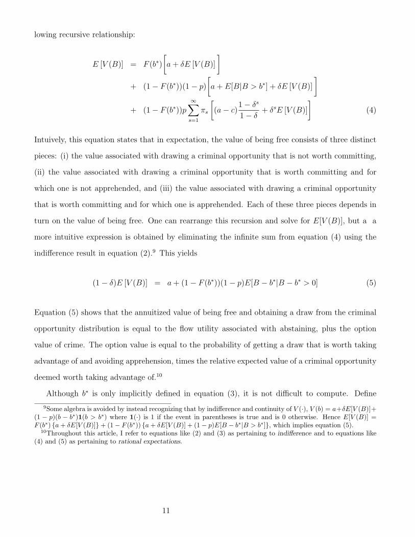
lowing recursive relationship:

E [V (B)] = F (b∗)

[a+ δE [V (B)]

]+ (1− F (b∗))(1− p)

[a+ E[B|B > b∗] + δE [V (B)]

]+ (1− F (b∗))p

∞∑s=1

πs

[(a− c)1− δs

1− δ+ δsE [V (B)]

](4)

Intuively, this equation states that in expectation, the value of being free consists of three distinct

pieces: (i) the value associated with drawing a criminal opportunity that is not worth committing,

(ii) the value associated with drawing a criminal opportunity that is worth committing and for

which one is not apprehended, and (iii) the value associated with drawing a criminal opportunity

that is worth committing and for which one is apprehended. Each of these three pieces depends in

turn on the value of being free. One can rearrange this recursion and solve for E[V (B)], but a a

more intuitive expression is obtained by eliminating the infinite sum from equation (4) using the

indifference result in equation (2).9 This yields

(1− δ)E [V (B)] = a+ (1− F (b∗))(1− p)E[B − b∗|B − b∗ > 0] (5)

Equation (5) shows that the annuitized value of being free and obtaining a draw from the criminal

opportunity distribution is equal to the flow utility associated with abstaining, plus the option

value of crime. The option value is equal to the probability of getting a draw that is worth taking

advantage of and avoiding apprehension, times the relative expected value of a criminal opportunity

deemed worth taking advantage of.10

Although b∗ is only implicitly defined in equation (3), it is not difficult to compute. Define

9Some algebra is avoided by instead recognizing that by indifference and continuity of V (·), V (b) = a+δE[V (B)]+(1 − p)(b − b∗)1(b > b∗) where 1(·) is 1 if the event in parentheses is true and is 0 otherwise. Hence E[V (B)] =F (b∗) {a+ δE[V (B)]}+ (1− F (b∗)) {a+ δE[V (B)] + (1− p)E[B − b∗|B > b∗]}, which implies equation (5).

10Throughout this article, I refer to equations like (2) and (3) as pertaining to indifference and to equations like(4) and (5) as pertaining to rational expectations.

11

ν =∑∞

s=1 πsδ−δs1−δ and the functions11

ψ(b) = (1− F (b))E [B − b|B − b > 0] =

∫ ∞b

(t− b)f(t)dt =

∫ ∞b

(1− F (t))dt (6)

ψ̃(b) = −F (b)E [B − b|B − b < 0] = −∫ b

0

(t− b)f(t)dt =

∫ b

0

F (t)dt (7)

Then, combining equations (3) and (5), we have

b∗ = cp

1− p

[1 + ν

(1 +

(1− p)ψ(b∗)

c

)]= α + βψ(b∗) (8)

=α + βE[B]

1 + β+

β

1 + βψ̃(b∗) ≡ α̃ + β̃ψ̃(b∗) (9)

where α = c p1−p (1 + ν) > 0, β = pν > 0, and where equation (9) follows from the fact that

ψ(b) = E[B] − b + ψ̃(b).12 Equations (8) and (9) can be used to demonstrate that b∗ is unique,

and equation (9) demonstrates the viability of solving for b∗ using a contraction mapping, since

β̃ < 1. That is, one can apply equation (9) repeatedly, starting at any initial guess for b∗, and be

guaranteed a solution in a finite number of steps. In practice, this usually only takes a few steps and

is easy to implement in standard software as part of a routine for evaluating a likelihood function

or a moment function.13

Figure 1 presents a graphical analysis of equations (8) and (9) for a particular parameterization

of the baseline model. In both panels, the x-axis is a possible value of the reservation benefit, or

b, and the solid line is the 45 degree line. In panel A, the dashed curve is α + βψ(b), which is

monotonically decreasing with a positive intercept for any criminal benefit distribution, and hence

guaranteed to cross the 45 degree line once and only once. In panel B, the dashed curve is α̃+β̃ψ̃(b),

which is monotonically increasing with a positive intercept. The uniqueness of the intersection then

follows since the derivative of α̃+ β̃ψ̃(b) is strictly less than one. In both figures, the vertical dotted

11Note that (1) ν is guaranteed to be between 0 and min{E[S] − 1, δ/

(1 − δ)}, is increasing in the severity ofsentences, can be rewritten as

∑∞s=1 δ

sP (S > s), and has derivative ∂ν∂δ =

∑∞s=1 sδ

s−1P (S > s) > 0; (2) ψ(·) is apositive, decreasing, convex function with ψ′(b) = −(1−F (b)), ψ′′(b) = f(b), ψ(0) = E[B], and limb→∞ ψ(b) = 0; and(3) ψ̃(·) is a positive, increasing, convex function with ψ̃′(b) = F (b), ψ̃′′(b) = f(b), ψ̃(0) = 0, and limb→∞ ψ̃(b) =∞.

12The fact that ψ(b) = E[B]− b+ ψ̃(b) can be seen by adding and subtracting∫ b0

(1− F (t))dt from the definitionfor ψ(b).

13A slightly faster approach is to apply Newton’s method to either equation (8) or (9). For a detailed discussionof computational issues in dynamic models from a more general perspective, see Rust (1996).

12

Figure 1. Reservation Benefit as Fixed Point:A. b∗ = α + βψ(b∗) and B. b∗ = α̃ + β̃ψ̃(b∗)

0.5

11.

52

2.5

0 .5 1 1.5 2 2.5

A.

0.5

11.

52

2.5

0 .5 1 1.5 2 2.5

B.

Note: Figures drawn using baseline model with a = 0, c = 1, δ = 0.95, p = 0.2, πs = (1 − γ)γs−1, with γ = e−1/5,and F (b) = 1− exp(−b).

line indicates the value of the reservation benefit, b∗.14

The ex ante probability of crime commission among those not detained is given by G(b∗) ≡

1−F (b∗). Thus, factors that work to increase b∗ work to decrease crime on the part of the undetained

population. We have the following results. Crime is unambiguously reduced by increases in: (1) δ,

the discount factor; (2) p, the probability of apprehension; and (3) c, the per period relative cost

of prison. This is because increasing any of these quantities increases α, which shifts out the

dashed curve α+ βψ(b). Increasing δ and p also increases β, which results in a further shift out in

α + βψ(b). Any shift out in this curve increases b∗ and hence decreases G(b∗), i.e., lowers the ex

ante probability of crime on the part of an undetained person.15 The remaining comparative statics

I consider pertain to distributions: that of sentence lengths, or {πs}∞s=1, and that of the criminal

benefit, or F (·). Regarding sentence lengths, we have the following result: as long as δ > 0, i.e., as

long as the agent cares about the future, any rightward (i.e., first order stochastic dominant) shift

in the distribution of sentence lengths unambiguously reduces crime. The easiest way to recognize

this is to note that any rightward shift in the distribution of sentence lengths increases P (S > s)

14This formulation shows

c p1−p (1 + ν) + pνE[B]

1 + pν< b∗ < c

p

1− p(1 + ν) + pνE[B]

which holds regardless of the criminal benefit distribution. These bounds are tight when pν is small.15These results can also be established rigorously using the implicit function theorem.

13

for at least one s. Since ν can be written as ν =∑∞

s=1 δsP (S > s), such a shift increases ν, which

increases β, shifting out α + βψ(b). Of course, when δ = 0, ν is exactly zero and does not respond

to changes to the distribution of sentences.

Regarding the distribution of criminal benefits, nothing general can be said about the effect of

a shift to the right in the distribution on the crime rate. This counterintuitive result (“Shouldn’t

there always be more crime when crime is worth more?”) is a distinctive feature of a dynamic model

of crime. The reason for the ambiguity of such a comparative static is that even though a shift to

the right increases b∗ unambiguously, by definition the survivor curve 1 − F (b) also shifts out. In

some settings, the shift out in the survivor function can fully offset the shift out in the reservation

benefit, resulting in a net reduction in crime.

To explain this issue, consider two examples of shifts to the right in the criminal benefit distri-

bution. The first example is associated with an increase in crime. For k > 1, the survivor function

1 − F (b) increases for values b > kb∗, but is the same for b ≤ kb∗. This leads to an increase in

the reservation benefit because ψ(·) mechanically increases (see equation (6)). However, since the

survivor function does not shift in the neighborhood of b∗, the survivor function is unaffected at the

new b∗, and the net effect is an increase in crime.

The second example is instead associated with a decrease in crime. The initial criminal benefit

distribution has support on [0, 1] and further has a mass point at 1. Let q denote the probability

that the benefit is exactly 1. Now consider a rightward shift in the distribution such that the mass

point is increased from 1 to B. Such a move necessarily increases b∗, and for large enough B moves

b∗ above 1. In this example, whenever b∗ moves above 1, the probability of crime on the part of the

free is immediately q, which can be arbitrarily small and hence lower than any original probability

of crime.

The intuition behind these two examples is as follows. When the criminal benefit distribution

shifts to the right, two conceptually different effects impinge on behavior: the current wage effect

and the opportunity cost effect. The current wage effect is that the value of crime is higher, which

would lead to more crime if E[V (B)] were held constant. The opportunity cost effect is that all

future draws are likely to be better than they otherwise would be: that is, E[V (B)] is higher.

Hence, committing crime next period puts the agent at risk of being imprisoned and hence unable

14

to avail himself of criminal opportunities two periods hence, three periods hence, and so on. The

opportunity cost effect tends to reduce crime. In the extreme, the opportunity cost effect can

dominate. Intuitively, we can imagine a shift in the distribution of criminal benefits such that there

is an outside chance at riches so fantastic that the agent chooses to spend the vast majority of his

life abstaining from crime, hoping to be free and able to avail himself of a criminal opportunity so

rare that it almost never arrives.

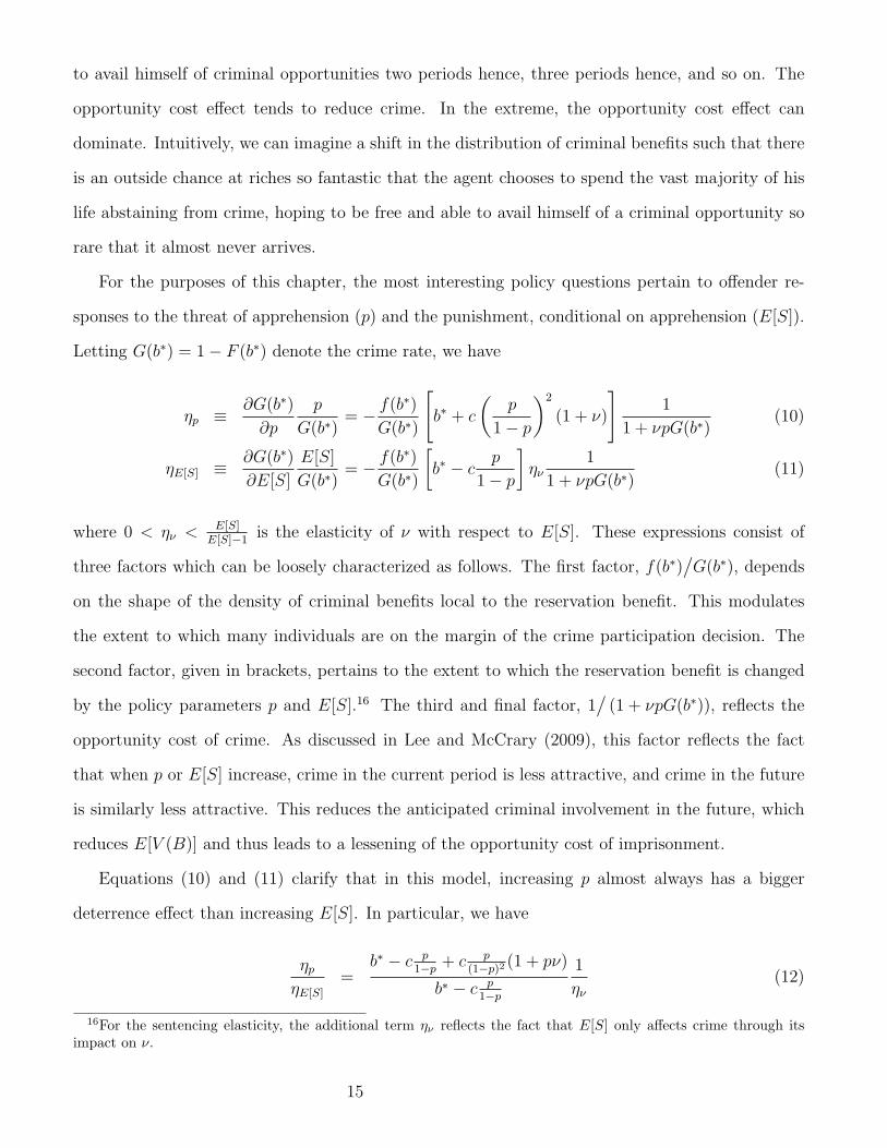
For the purposes of this chapter, the most interesting policy questions pertain to offender re-

sponses to the threat of apprehension (p) and the punishment, conditional on apprehension (E[S]).

Letting G(b∗) = 1− F (b∗) denote the crime rate, we have

ηp ≡∂G(b∗)

∂p

p

G(b∗)= − f(b∗)

G(b∗)

[b∗ + c

(p

1− p

)2

(1 + ν)

]1

1 + νpG(b∗)(10)

ηE[S] ≡∂G(b∗)

∂E[S]

E[S]

G(b∗)= − f(b∗)

G(b∗)

[b∗ − c p

1− p

]ην

1

1 + νpG(b∗)(11)

where 0 < ην <E[S]E[S]−1

is the elasticity of ν with respect to E[S]. These expressions consist of

three factors which can be loosely characterized as follows. The first factor, f(b∗)/G(b∗), depends

on the shape of the density of criminal benefits local to the reservation benefit. This modulates

the extent to which many individuals are on the margin of the crime participation decision. The

second factor, given in brackets, pertains to the extent to which the reservation benefit is changed

by the policy parameters p and E[S].16 The third and final factor, 1/

(1 + νpG(b∗)), reflects the

opportunity cost of crime. As discussed in Lee and McCrary (2009), this factor reflects the fact

that when p or E[S] increase, crime in the current period is less attractive, and crime in the future

is similarly less attractive. This reduces the anticipated criminal involvement in the future, which

reduces E[V (B)] and thus leads to a lessening of the opportunity cost of imprisonment.

Equations (10) and (11) clarify that in this model, increasing p almost always has a bigger

deterrence effect than increasing E[S]. In particular, we have

ηpηE[S]

=b∗ − c p

1−p + c p(1−p)2 (1 + pν)

b∗ − c p1−p

1

ην(12)

16For the sentencing elasticity, the additional term ην reflects the fact that E[S] only affects crime through itsimpact on ν.

15

The first term,b∗−c p

1−p+c p

(1−p)2(1+pν)

b∗−c p1−p

, always exceeds 1, and the second term, 1ην

, exceeds 1 except for

arbitrarily patient individuals facing short expected sentence lengths.

B . Heterogeneity

Assumptions of time homogeneity are restrictive for most crime applications, due to the rapid

changes in criminal involvement as youths move into adulthood (Lochner 2004). Similarly, the

literature has emphasized the cross-sectional heterogeneity in criminal propensity, with a small

number of individuals committing a great number of crimes (Visher 1986, Piehl and DiIulio 1995,

Blumstein 2002).

When the flow utilities vary over time and across persons, the model is similar, but the notation

becomes more complicated, and careful attention must be paid to the nature of conditional inde-

pendence assumptions which are invoked. Let Fi,t|t−j(b) denote the distribution function associated

with the criminal benefit for agent i in period t, Bit, conditional on information on agent i available

as of period t − j, j > 0. For j = 0, we write Fit|t(b) ≡ Fit(b). Let pit|t−j denote the probability

of apprehension in period t, conditional on having committed crime in period t and conditional on

information regarding the agent available at the beginning of period t− j, and write pit|t ≡ pit.17

It is now important to recall the timing convention of the model: (1) at the beginning of period t,

the agent forms beliefs for pit, πits, and expectations of future flow utilities and the values of the

dynamic program, and chooses b∗it, (2) the criminal benefit Bit is revealed to agent i, (3) the agent

chooses whether to engage in crime or not, and (4) if the agent decided to commit crime in stage

3, then apprehension may or may not occur.

If agent i elects in period t to engage in a crime of value Bit = bit and gets away with it,

he receives payoff ait + bit + Eit[Vi,t+1(Bi,t+1)], where Eit[·] is the expectation operator conditional

on information regarding agent i available at period t.18 If the agent is instead apprehended, he

17I abstract from the possibility that the probability of apprehension and the sentence may depend on the value ofcrime. This would be an interesting extension of the model. Viscusi (1986) argues that crimes of greater value areassociated with greater probabilities of apprehension.

18If there are state variables, then Eit[·] is an expectation conditional on those state variables, as of period t.

16

receives, with probability πits, the sentence s and the payoff

Eit[(ait − cit) + δ(ai,t+1 − ci,t+1) + · · ·+ δs−1(ai,t+s−1 − ci,t+s−1) + δsVi,t+s(Bi,t+s)] (13)

If the agent abstains from crime, he receives the payoff ait + δEit[Vi,t+1(Bi,t+1)]. Thus, the value to

agent i of being free in period t and receiving criminal opportunity Bit = b is

Vit(b) = max

{ait + δEit[Vi,t+1(Bi,t+1)] , (14)

pit

∞∑s=1

πitsEit

[s−1∑j=0

δj(ai,t+j − ci,t+j) + δsVi,t+s(Bi,t+s)

]

+(1− pit)(ait + b+ δEit [Vi,t+1(Bi,t+1)]

)}= ait + δEit [Vi,t+1(Bi,t+1)] + (1− pit)(b− b∗it)1(b > b∗it) (15)

where the simplification in equation (15) occurs by the same reasoning described for the baseline

model, and where the reservation benefit is given by

b∗it =pit

1− pit

{ait + δEit [Vi,t+1(Bi,t+1)]−

∞∑s=1

πitsEit

[s−1∑j=0

δj(ai,t+j − ci,t+j) + δsVi,t+s(Bi,t+s)

]}(16)

The indifference equation (16) indicates that b∗it depends on expectations of future utility flows and

values of the dynamic program. From the rational expectations equation (15), we see that

Ei,t−1[Vit(Bit)]− δEi,t−1[Vi,t+1(Bi,t+1)] = Ei,t−1[ait] + Ei,t−1[(1− pit)(Bit − b∗it)1(Bit > b∗it)] (17)

As in the baseline model, the indifference and rational expectations equations (16) and (17)

are the main equations of this model. Precisely how to form the relevant expectations differs

substantially across variations of this model. For these models to be tractable, sufficient structure

has to be placed on flow utilities, system variables, and laws of motion that equations (16) and

(17) can be solved. The literature is sufficiently in its infancy that there has not yet emerged a

“workhorse” model, so assumptions differ.

17

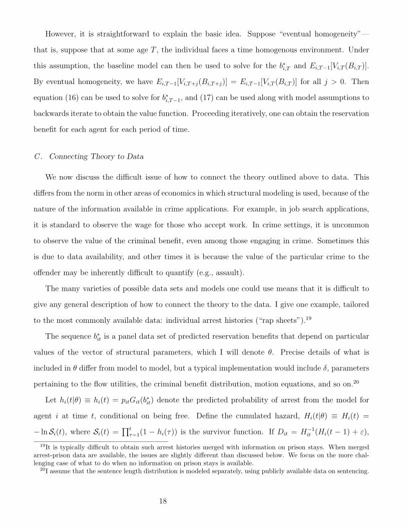
However, it is straightforward to explain the basic idea. Suppose “eventual homogeneity”—

that is, suppose that at some age T , the individual faces a time homogenous environment. Under

this assumption, the baseline model can then be used to solve for the b∗i,T and Ei,T−1[Vi,T (Bi,T )].

By eventual homogeneity, we have Ei,T−1[Vi,T+j(Bi,T+j)] = Ei,T−1[Vi,T (Bi,T )] for all j > 0. Then

equation (16) can be used to solve for b∗i,T−1, and (17) can be used along with model assumptions to

backwards iterate to obtain the value function. Proceeding iteratively, one can obtain the reservation

benefit for each agent for each period of time.

C . Connecting Theory to Data

We now discuss the difficult issue of how to connect the theory outlined above to data. This

differs from the norm in other areas of economics in which structural modeling is used, because of the

nature of the information available in crime applications. For example, in job search applications,

it is standard to observe the wage for those who accept work. In crime settings, it is uncommon

to observe the value of the criminal benefit, even among those engaging in crime. Sometimes this

is due to data availability, and other times it is because the value of the particular crime to the

offender may be inherently difficult to quantify (e.g., assault).

The many varieties of possible data sets and models one could use means that it is difficult to

give any general description of how to connect the theory to the data. I give one example, tailored

to the most commonly available data: individual arrest histories (“rap sheets”).19

The sequence b∗it is a panel data set of predicted reservation benefits that depend on particular

values of the vector of structural parameters, which I will denote θ. Precise details of what is

included in θ differ from model to model, but a typical implementation would include δ, parameters

pertaining to the flow utilities, the criminal benefit distribution, motion equations, and so on.20

Let hi(t|θ) ≡ hi(t) = pitGit(b∗it) denote the predicted probability of arrest from the model for

agent i at time t, conditional on being free. Define the cumulated hazard, Hi(t|θ) ≡ Hi(t) =

− lnSi(t), where Si(t) =∏t

τ=1(1 − hi(τ)) is the survivor function. If Dit = H−1it (Hi(t − 1) + ε),

19It is typically difficult to obtain such arrest histories merged with information on prison stays. When mergedarrest-prison data are available, the issues are slightly different than discussed below. We focus on the more chal-lenging case of what to do when no information on prison stays is available.

20I assume that the sentence length distribution is modeled separately, using publicly available data on sentencing.

18

where H−1it (v) ≡ min{t : Hi(t) ≥ v} and ε is distributed standard exponential, then Dit is a duration

consistent with the hazard sequence hi(t|θ), hi(t + 1|θ), . . . (Devroye 1986, Section VI.2). That is,

Dit is a duration consistent with being at risk of failure starting in period t.21

Let Xi denote age at first arrest, and let Y ∗i denote age at second arrest. I use the notation

Y ∗i because age at second arrest may be censored. Under the model, age at second arrest may be

viewed as having been generated as

Y ∗i = H−1(H(Xi + Si − 1) + εi) (18)

where Xi is age at first arrest, Si is sentence length, and εi is distributed standard exponential and

independent of Xi and Si.

I next use this representation to derive the log-likelihood function for observed age at second

arrest, conditional on age at first arrest. To do so, I first derive the distribution of (latent) age at

second arrest and then apply standard results on likelihood functions under censoring. Fix y > Xi,

both integers. The event Y ∗i ≤ y is the same as the event H(Xi+Si−1)+εi ≤ H(y), and the event

Y ∗i = y is the same as the event H(y− 1) < H(Xi + Si − 1) + εi ≤ H(y). This leads to expressions

for the conditional distribution function and conditional probability function of Y ∗i ,

FY ∗|X(y|Xi) =∞∑s=1

P (Si = s|Xi)E(H(y)−H(Xi + s− 1))

= P (Si ≤ y −Xi|Xi)−y−Xi∑s=1

P (Si = s|Xi)S(y)/S(Xi + s− 1) (19)

fY ∗|X(y|Xi) =∞∑s=1

P (Si = s|Xi){E(H(y)−H(Xi + s− 1))− E(H(y − 1)−H(Xi + s− 1))

}= h(y)

y−Xi∑s=1

P (Si = s|Xi)S(y − 1)/S(Xi + s− 1) (20)

where E(t) = max{0, 1− exp(−t)} is the distribution function for the standard exponential distri-

bution. One may verify that equation (20) is the first difference of equation (19). Both expressions

can be calculated exactly given a known conditional distribution for sentences given age at first

21There is no content to ε being distributed standard exponential. Rather, this is simply the duration data analogueto the well-known result that F (Z) is distributed standard uniform, if Z has distribution function F (·).

19

arrest.

Observed age at second arrest is a censored version of latent age at second arrest, i.e., Yi =

min{Y ∗i , Ci}. This poses little difficulty once we have specified the distribution of the latent variable,

however (Wooldridge 2002, Lawless 2003). Let κi = 1 indicate that the observation is censored and

κi = 0 indicate that it is not. Then the log-likelihood function is

L(θ) ≡ 1

n

n∑i=1

Li(θ) =1

n

n∑i=1

{(1− κi) ln fY ∗|X(Yi|Xi) + κi ln

(1− FY ∗|X(Ci|Xi)

)}(21)

Most software packages allow the user to pass a function of data and parameters to a maxi-

mization routine that determines the parameter values that maximize the function, given the data.

Passing L(θ) to such a maximization routine is thus a straightforward approach that yields maxi-

mum likelihood estimates of θ. The only computational problems with such an approach are that,

depending on the scope of the data set and the model, it can be slow to evaluate the function L(θ).

Note that analytical derivatives of the likelihood function are extremely tedious to compute and

likely not worth the effort, except in special cases. Consequently, the user will likely find it optimal

to use numerical derivatives, which means many, many more function evaluations will be required

before the routine has climbed to the top of the likelihood function.22

While I have discussed estimation by maximum likelihood in this subsection, this is certainly

not the only available method for connecting the theory to the data. A leading technique is to

choose a set of empirical quantities which are implicated by the structural parameters of interest.

As long as there are a sufficient number of moments, one can hope to judiciously vary the structural

parameters to match those moments.

This approach has the advantage that the economist can choose which moments to match.

Obtaining and interpreting the score in dynamic crime models, even for the simplest versions,

is costly; although it can be done, I am aware of no results in the literature along these lines.

This means it is hard to describe intuitively the essential source of the identifying information in

the data. Hence, it can be hard to assess the credibility of structural estimates from maximum

likelihood. Choosing a set of moments that are to be matched by judicious choice of structural

22A further consideration is the impact of computer precision on these function evaluations. For an introductorydiscussion, see Judd (1998). In my experience, these issues are particularly relevant for approximating infinite sums.

20

parameters clarifies the essential identifying information in the data; it is the moments themselves.

For example, Lee and McCrary (2009) use the change in offense rates around the 18th birthday to

generate quasi-experimental moments.23

IV. Government

In this section, I consider the government’s problem instead of the offender’s problem. Government

decides what level of resources should be devoted to fighting crime and how to use those resources

within the criminal justice system. Expenditures on police and other uses are related to the “system

parameters” discussed in Section III. When government hires additional police officers, it does so

with the aim of increasing the probability of apprehension, or p. When arrests per officer is only

negligibly affected by the number of officers, then a 5 percent increase in the number of officers

is associated with a 5 percent increase in p. When government passes laws for sentence enhance-

ments, abolishment of parole, mandatory minimum sentences, and so on, it shifts the distribution

of detention times for an arrestee to the right. Thus, a reasonable approximation to the problem

facing government is minimization of the present discounted value of the crime burden by judicious

choice of pt and P (St ≥ s), subject to an intertemporal budget constraint.

This suggests the following formalization of the government’s problem:

min{pt,P (St≥s)}∞t=0

E0

[∞∑t=0

βtCt

]s.t. At+1 = Rt+1(At + It −Bt) and At ≥ A (22)

Here, pt is the aggregate apprehension probability, P (St ≥ s) is the aggregate survivor function for

a sentence length, β summarizes the government’s taste for the present, Ct is the probability that

a person selected at random at time t from among the entire population (both free and in prison)

is engaged in crime, At is criminal justice “assets”, A is a minimum level of assets below which

government cannot go, It is criminal justice revenues, Bt is per capita criminal justice expenditures,

and Rt+1 is the gross return to assets between periods t and t+ 1. Below, we will make use of the

notation Qt, or the probability that a person selected at random at time t is in prison. Although

23An interesting technical issue that can arise in this context is that because of the nonlinearity of dynamic model,some moments that can be observed may not within the range of the model. This can often be remedied by minoralterations to the model, but it is not always obvious how the model needs to be altered.

21

Ct and Qt are probabilities, it is useful to think of these terms as capturing crime per capita and

prisoners per capita, respectively.

Both crime per capita and criminal justice expenditures per capita are related to prisoners per

capita. Since prisoners per capita is a stock, the flow rate into and out of prison dictates the level.

These considerations lead to the restrictions

Ct = (1−Qt)Gt (23)

Bt = wtpt + rtQt (24)

Qt = (1−Qt−1)Gt−1pt−1 +Qt−1(1−Xt−1) (25)

where Gt is the probability of crime on the part of someone not in prison, wtpt is the per capita

apprehension (“policing”) budget, rtQt is the per capita sentence length (“corrections”) budget,

and Xt is the exit rate of a prisoner selected at random in period t (cf., Raphael and Stoll 2009).24

I will refer to equations (23), (24), and (25) as the crime equation, the budget equation, and the

prison equation, respectively.

The crime equation clarifies that crime is mechanically reduced by imprisonment; this is the

incapacitation effect of prison that is discussed in the literature. The budget equation clarifies that

governments must pay for furnishing a probability of apprehension, regardless of whether the crime

rate is high or low. However, governments do not have to pay for long prison sentences if crime falls

by enough to keep prison populations low.25 Intuitively, the most effective punishment is the one

that never needs to be carried out. This idea, immediately recognized by every parent, is quite old

in the crime literature and dates at least to Bentham (1789).26

At first blush, it seems that if we impose parametric assumptions on the sentence length dis-

tribution so that P (St ≥ s) is a function of a finite number of parameters, then this problem can

be solved analytically with standard recursive methods.27 This is somewhat illusory, however. To

24For the purposes of the theory described here, I consider judicial expenditures part of the corrections budget. Itis useful to think of wt as the price of an arrest and rt as the price of incarcerating a person for a year. For example,if the typical police officer arrests 10 people a year and costs the government $100,000 in wages, benefits, and so on,then wt = $10, 000. A typical estimate of rt is $20,000 (Bureau of Justice Statistics 2004).

25Dan Nagin pointed out to me that this issue was treated formally in Blumstein and Nagin (1978).26A more recent discussion, with many interesting examples, is given by Kleiman (2009).27For an introduction to recursive methods, see Adda and Cooper (2003).

22

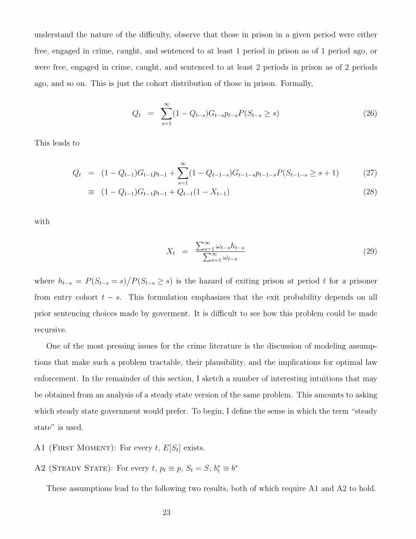
understand the nature of the difficulty, observe that those in prison in a given period were either

free, engaged in crime, caught, and sentenced to at least 1 period in prison as of 1 period ago, or

were free, engaged in crime, caught, and sentenced to at least 2 periods in prison as of 2 periods

ago, and so on. This is just the cohort distribution of those in prison. Formally,

Qt =∞∑s=1

(1−Qt−s)Gt−spt−sP (St−s ≥ s) (26)

This leads to

Qt = (1−Qt−1)Gt−1pt−1 +∞∑s=1

(1−Qt−1−s)Gt−1−spt−1−sP (St−1−s ≥ s+ 1) (27)

≡ (1−Qt−1)Gt−1pt−1 +Qt−1(1−Xt−1) (28)

with

Xt =

∑∞s=1 ωt−sht−s∑∞s=1 ωt−s

(29)

where ht−s = P (St−s = s)/P (St−s ≥ s) is the hazard of exiting prison at period t for a prisoner

from entry cohort t − s. This formulation emphasizes that the exit probability depends on all

prior sentencing choices made by goverment. It is difficult to see how this problem could be made

recursive.

One of the most pressing issues for the crime literature is the discussion of modeling assump-

tions that make such a problem tractable, their plausibility, and the implications for optimal law

enforcement. In the remainder of this section, I sketch a number of interesting intuitions that may

be obtained from an analysis of a steady state version of the same problem. This amounts to asking

which steady state government would prefer. To begin, I define the sense in which the term “steady

state” is used.

A1 (First Moment): For every t, E[St] exists.

A2 (Steady State): For every t, pt ≡ p, St = S, b∗t ≡ b∗

These assumptions lead to the following two results, both of which require A1 and A2 to hold.

23

Result 1: Qt ≡ Q = AE[S]/

(1 + AE[S]), where E[S] is the expected sentence length.

Proof: In steady state, we have Q = (1−Q)A∑∞

s=1 P (S ≥ s) = (1−Q)AE[S], where the result∑∞s=1 P (S ≥ s) = E[S] follows from rearrangement of the terms of the implicit triangular sum.

Rearrangement does not affect the limit since all terms are non-negative. �

Result 2: Ct ≡ C = G/

(1 +GpE[S]), where Ct denotes the number of crimes per person. Thisimplies that Q = CpE[S]: the fraction of people in prison equals the probability of crime, timesthe probability of arrest, times the expected number of periods detained.

Proof: We have C = (1−Q)G. By Result 1, we have 1−Q = 1/(1 +GpE[S]). �

An important use of Results 1 and 2 is a decomposition of crime elasticities with respect to p

and E[S] into deterrence and incapacitation components.

Result 3: In steady state, (i) the elasticity of crime with respect to the probability of apprehensioncan be decomposed into deterrence and incapacitation components; (ii) the elasticity of crime withrespect to the expected sentence length can be likewise decomposed; and (iii) the incapacitationcomponents are equal. Formally,

εp =∂C

∂p

p

C= (1−Q)

∂G

∂p

p

G−Q ⇐⇒ εp = (1−Q)ηp −Q

εE[S] =∂C

∂E[S]

E[S]

C= (1−Q)

∂G

∂E[S]

E[S]

G−Q ⇐⇒ εE[S] = (1−Q)ηE[S] −Q

Proof: Follows from Results 1 and 2, calculus, and algebra. �

Result 3 means that the overall crime elasticities, εE[S] and εp, are both weighted averages

of the deterrence elasticities, ηE[S] and ηp, and an incapacitation elasticity of -1. The weights in

the decomposition are 1 − Q and Q. Moreover, Result 3 indicates that incapacitation effects are

equal for p and E[S]. Thus, incapacitation is never a good argument for allocating the marginal

criminal justice dollar to funding sentence enhancements instead of improvements to the probability

of apprehension—the same incapacitation benefit could be generated by spending more money on

increasing the probability of apprehension, such as by increasing funding for police.28 Intuitively,

prisoners must first be apprehended before they can be incapacitated by prison.

In steady state, government cannot run a deficit and simply spends a constant amount each

period. This simplifies the governments problem to the optimal allocation of criminal justice ex-

penditures between providing a probability of apprehension and expected punishment conditional

28Additional mechanisms for increasing p through government investments include parole officers, informationtechnology, state and federal crime labs, and so on.

24

on apprehension:

minp,E[S]

C s.t. E ≤ E0 (30)

where E = wp + rCpE[S] is steady state expenditures, C is steady state crime, and E0 is the

maximum budget.

A standard conclusion from microeconomic theory is that any interior solution to such a problem

can be characterized as

∂C∂p

pC

∂C∂E[S]

E[S]C

=εpεE[S]

=

∂E∂p

pE

∂E∂E[S]

E[S]E

In words, the crime reducing benefit of spending 1 percent more on expected sentence lengths must

be equal to the crime reducing benefit of spending 1 percent more on the probability of apprehension.

This is the elasticity form of the classic conclusion that the marginal benefit of increased spending

on any given budget item must equal the marginal benefit of increased spending on any other budget

item.

In addition to the interior solutions to this problem, there are also corner solutions. Abstract

from the corner solutions analogous to quasilinear preferences in consumer theory.29 There are also

more interesting corner solutions that are associated with the nonlinearity of the government budget

constraint. These nonlinearities are due to the fact that the crime rate, C, enters the government

budget constraint directly, due to the influence of the crime rate on the prison population (Blumstein

and Nagin 1978).

To develop this idea, observe that the percentage increase in expenditures, given a percentage

increase in p and E[S], is

∂E

p

p

E= 1 + (1− σ)εp (31)

∂E

∂E[S]

E[S]

E= (1− σ)(1 + εE[S]) (32)

29A formal characterization of when it is reasonable to rule out corner solutions of this type would take me farafield. Any formal model of behavior, such as the model outlined in Section II can be adopted to provide such acharacterization.

25

where σ = wpE

is the policing share of the criminal justice budget, and note that both of these

quantities can be negative—that is, for both p and E[S], the investments can be self financing.

This result stands in contrast with the standard linear budget, where both budget elasticities

are exactly equal to 1. Here, the budget elasticities are smaller than 1, because of the possibility

that crime is reduced by the government’s increased punishment. If crime is reduced enough, then

both budget elasticities are negative. Thus, under a maintained assumption of cost minimization

on the part of government, we should not expect to observe crime elasticities of large magnitude. If

they were to exist, arguendo, then government would have recognized that crime could be lowered

and money could be saved, by investing more. On the other hand, when cost minimization is not

a maintained assumption, this kind of reasoning suggests an avenue for substantial government

savings.

Increasing the probability of apprehension will save money if εp <−11−σ , or equivalently if ηp <

−1(1−σ)(1−Q)

+ Q1−Q . Increasing expected sentence lengths will save money if εE[S] < −1, or equivalently

if ηE[S] < −1. That is, if offenders exhibit elastic behavior with respect to sentences, then increasing

sentence lengths lowers crime and lowers government cost.

There is also a further corner solution that arises due to the nonlinear budget. This occurs when

offenders are more responsive to a 1 percent increase in E[S] than they are to a 1 percent increase in

p, or when |εE[S]| > |εp|. However, it is hard to imagine that behavior is more elastic with respect to

sentences than the probability of apprehension, regardless of p and E[S]. More plausibly, behavior

is more elastic with respect to the probability of apprehension, and increasingly so when sentences

become long. For example, plausible calibrations of equations (10) and (11) suggest strong the

probability of apprehension and sentence lengths and thus the implausibility of this type of corner

solution.

Returning to the characterization of an interior solution, we see that at an interior optimum,

the fraction of the criminal justice budget that should be devoted to policing is given by

σ = 1−εE[S]

εp(33)

Armed with estimates of deterrence elasticities, this equation gives a simple formula for optimal

26

allocation of government resources.

Figure 2. Policing Budget Share, or σ: 1971-2005

.4.4

5.5

.55

.6

1970 1980 1990 2000

Source: Bureau of Justice Statistics, Expenditure and Employment Series

Figure 2 shows the time series of federal, state, and local criminal justice expenditures devoted

to non-policing sources (i.e., judicial expenses are here viewed as part of detention rather than

apprehension). The figure shows plainly the increased criminal justice focus on detention rather

than apprehension over the past 40 years, particularly in the period 1970-1995.

Equation (33) shows that, maintaining the hypothesis that the federalist system achieves cost

minimization, policing must have become less effective over this period. To understand the mag-

nitude of the implied effect, suppose that arrests per officer are constant. Then in 1970, equation

(33) shows that the hypothesis of cost minimization implies an elasticity of crime with respect to

police, relative to that with respect to sentence lengths, of about 2.5. If cost minimization were

true, then it must be the case that over the period 1970-2005, the elasticity of policing, relative to

that of sentence lengths, fell from 2.5 to about 1.8, or a decline of about one-third. To the extent

that such a decline seems implausible, it suggests that either money could currently be saved by

reallocating spending away from prisons and towards police, or that money could historically have

been saved by reallocating spending away from police and towards prison.

If potential criminals are completely unresponsive to punishment parameters, so that εK

and

εE[S]

are both zero, then the government’s problem as stated is ill-posed: it then always makes sense

27

to maximize the size of the prison population, and for a fixed budget, this is always most efficiently

done by cutting police and increasing E[S]. The government’s problem would also be ill-posed if, in

the current environment, the elasticity of crime with respect to sentence lengths were elastic, i.e., if

ηE[S]

< −1.30 Under such a scenario, equation (32) shows that increasing sentences is self-funding.

The hypothesis of cost minimization thus implies an inelastic response of crime to expected sentence

lengths.

The steady state calculations above are helpful in understanding the incentives facing govern-

ments, but miss a key dynamic insight. Consider a government facing a crime wave and trying

to get under control using either police or the threat of prisons. As emphasized by equation (24),

increasing police in period t generates deterrence in period t, but also costs in period t. In contrast,

increasing sentence lengths in period t generates deterrence in period t, but costs are not borne

until period t + 1 and do not become large until Qt becomes large, frequently many periods later.

As discussed in Klick and Tabarrok (2005), for example, the three-strikes law passed in California

in 1994 sentenced a large number of offenders to 25 years to life instead of the typical sentence

of 10 years. Passing three-strikes thus postponed paying for crime control for 10 years. This is

presumably nearly always an attractive option for a state government facing a balanced budget

requirement.

V. Conclusion

Many interesting features of crime and crime control are dynamic in nature. In recent years, a

small literature has emerged that addresses some of these issues. Key areas of focus in the existing

literature include (1) the difficulty of controlling, via changes to sentencing, the criminal involvement

of those with short time horizons; (2) the intertemporal substitution of criminal activity; (3) the

accumulation of human capital, both criminal and legitimate, that can lead to important differences

between short- and long-run crime reduction benefits of policy interventions.

An important dynamic feature of crime that deserves more attention is the government’s problem

of how best to allocate criminal justice expenditures over time and between uses. This issue has

30Equivalently, if εE[S] < −1.

28

acquired a renewed relevance this past year with many governments seeking to cut costs in the wake

of the financial crisis. A particularly compelling question is the optimal division of criminal justice

dollars between police and prisons. I have emphasized that the government’s solution to this problem

relates to time preferences for marginal offenders, which powerfully influence the relative elasticities

of crime with respect to the probability of apprehension and with respect to an expected sentence

length. The United States has substantially reduced the fraction of criminal justice dollars devoted

to policing over the last 40 years and devoted the marginal dollar instead to corrections expenses.

If the marginal offender has short time horizons, then this may well not be the most efficient use of

the marginal criminal justice dollar, suggesting the possibility of substantial government savings.

A final issue which I suspect is an important future research direction is inducing criminals to

provide information to government that is useful for crime control. Currently, punishments depend

primarily criminal history and, to a lesser extent, judicial discretion. An interesting question is

whether government can elicit offender beliefs about the likelihood of recidivism. Assuming those

beliefs are accurate, such information could be highly valuable. For example, several states are

currently considering engaging in release of prisoners. A natural question is who should be released.

A natural answer is those with low probabilities of recidivism, but it is hard to know who those

prisoners are. One example of a policy that could be used to elicit beliefs about recidivism proba-

bilities is as follows. Those with 1 year left on their sentence are offered early release, contingent

upon being willing to wear an ankle bracelet. An offender anticipating recidivating might be loathe

to agree to such terms, because facing a higher probability of apprehension could lead to a longer

prison term than 1 year. Economists have not yet begun to carefully think about what kinds of

information revelation policies would be useful for government crime control, but we should be at

the forefront of such efforts.

29

References

Adda, Jerome and Russell W. Cooper, Dynamic Economics: Quantitative Methods and Applica-tions, Cambridge: MIT Press, 2003.

Becker, Gary S., “Crime and Punishment: An Economic Approach,” Journal of Political Economy,March/April 1968, 76 (2), 169–217.

Bentham, Jeremy, An Introduction to the Principles of Morals and Legislation, Oxford: ClarendonPress, 1789.

Blinder, Alan, “Wage Discrimination: Reduced Form and Structural Estimates,” Journal of HumanResources, 1973, 8 (4), 436–455.

Blumstein, Alfred, “Crime Modeling,” Operations Research, January-February 2002, 50 (1), 16–24.

and Daniel Nagin, “On the Optimum Use of Incarceration for Crime Control,” OperationsResearch, May-June 1978, 26 (3), 381–405.

Braga, Anthony, “Hot Spots Policing and Crime Prevention: A Systematic Review of RandomizedControlled Trials,” Journal of Experimental Criminology, September 2005, 1 (3).

Burdett, Kenneth, Ricardo Lagos, and Randall Wright, “Crime, Inequality, and Unemployment,”American Economic Review, December 2003, 93 (5), 1764–1777.

, , and , “An On-the-Job Search Model of Crime, Inequality, and Unemployment,”International Economic Review, August 2004, 45 (3), 681–706.

Bureau of Justice Statistics, “State Prison Expenditures, 2001,” Bureau of Justice Statistics SpecialReport, NCJ-202949, June 2004.

Cohen, Jacqueline, “Appendix B. Research on Criminal Careers: Individual Frequency Rates andOffense Seriousness,” in Alfred Blumstein, Jacqueline Cohen, Jeffrey A. Roth, and Christy A.Visher, eds., Criminal Careers and “Career Criminals”, Vol. 1, Washington, D.C.: NationalAcademy Press, 1986, pp. 292–418.

Devroye, Luc, Non-Uniform Random Variate Generation, New York: Springer-Verlag, 1986.

Di Tella, Rafael and Ernesto Schargrodsky, “Do Police Reduce Crime? Estimates Using theAllocation of Police Forces After a Terrorist Attack,” American Economic Review, March2004, 94 (1), 115–133.

DiNardo, John E., Nicole M. Fortin, and Thomas Lemieux, “Labor Market Institutions and theDistribution of Wages, 1973-1992: A Semiparametric Approach,” Econometrica, September1996, 64 (5), 1001–1044.

Eiserer, Tanya, “Police to Create Task Force to Combat Crime Hot Spots Effort to Start in EarlyJuly with About 60 Officers,” Dallas Morning News, June 11, 2005.

Flinn, Christopher, “Dynamic Models of Criminal Careers,” in Alfred Blumstein, Jacqueline Cohen,Jeffrey A. Roth, and Christy A. Visher, eds., Criminal Careers and “Career Criminals”, Vol. 2,Washington, D.C.: National Academy Press, 1986, pp. 356–379.

30

Glaeser, Edward L., Bruce Sacerdote, and Jose A. Scheinkman, “Crime and Social Interactions,”Quarterly Journal of Economics, May 1996, 111 (2), 507–548.

Grogger, Jeff, “Market Wages and Youth Crime,” Journal of Labor Economics, October 1998, 16(4), 756–791.

Gronau, Reuben, “Leisure, Home Production, and Work: The Theory of the Allocation of TimeRevisited,” Journal of Political Economy, December 1977, 85 (6), 1099–1123.

Heinzmann, David, “Murders Drop, but Chicago Leads U.S. ; Rate Down Sharply in Last 6Months,” Chicago Tribune, January 1, 2004.

Higgins, John, “City Police to Step up Presence: Mayor Adds $200,000 in Overtime to Target HotSpots, Enforce Curfew,” Akron Beacon Journal, August 2, 2006.

Hoover, Mike, “Sweeping Away Crime; Cooling Down Hot Spots for Blight; Sweeping Away theCrime; City Cops Try to Rid Area of Rroubles, but Residents Don’t Think It’s Enough,” York(PA) Daily Record, August 5, 2007.

Huang, Chien-Chieh, Derek Laing, and Ping Wang, “Crime and Poverty: A Search-TheoreticApproach,” International Economic Review, August 2004, 45 (3), 909–938.

Hunt, Amber, “Task Force Aims to Cool Down Crime Hot Spots in Detroit,” Detroit Free Press,August 12, 2009.

Imai, Susumu and Kala Krishna, “Employment, Deterrence, and Crime in a Dynamic Model,”International Economic Review, August 2004, 45 (3), 845–872.

Imrohoroglu, Ayse, Antonio Merlo, and Peter Rupert, “What Accounts for the Decline in Crime?,”International Economic Review, August 2004, 45 (3), 707–729.

Jacob, Brian, Lars Lefgren, and Enrico Moretti, “The Dynamics of Criminal Behavior: Evidencefrom Weather Shocks,” Journal of Human Resources, 2007, 42 (3), 489–527.

Judd, Kenneth L., Numerical Methods in Economics, Cambridge: MIT Press, 1998.

Katz, Matt, “Camden’s New Policing Style is Both Loved, Hated,” Philadelphia Inquirer, August9, 2009.

Kleiman, Mark, When Brute Force Fails: Strategy for Crime Control, Princeton: Princeton Uni-versity Press, 2009.

Klick, Jonathan and Alexander Tabarrok, “Using Terror Alert Levels to Estimate the Effect ofPolice on Crime,” Journal of Law and Economics, April 2005, 48.

Lawless, Jerald F., Statistical Models and Methods for Lifetime Data, Hoboken: John Wiley andSons, 2003.

Lee, David S. and Justin McCrary, “Crime, Punishment, and Myopia,” NBER Working Paper# 11491, July 2005.

and , “The Deterrence Effect of Prison,” July 2009. Unpublished manuscript, UCBerkeley.

31

Lemieux, Thomas, Bernard Fortin, and Pierre Frechette, “The Effect of Taxes on Labor Supply inthe Underground Economy,” American Economic Review, March 1994, 84 (1), 231–254.

Ljungqvist, Lars and Thomas J. Sargent, Recursive Macroeconomic Theory, Cambridge: MITPress, 2004.

Lochner, Lance, “Education, Work, and Crime: A Human Capital Approach,” International Eco-nomic Review, August 2004, 45 (3), 811–843.

McCall, John J., “Economics of Information and Job Search,” Quarterly Journal of Economics,1970, 84 (1), 113–126.

Oaxaca, R., “Male-female wage differentials in urban labor markets,” International EconomicReview, 1973, 14, 693–709.

Piehl, Anne Morrison and John J. DiIulio Jr., “‘Does Prison Pay?’ Revisited: Returning to theCrime Scene,” Brookings Review, Winter 1995, pp. 21–25.

Raghavan, Sudarsan, “Johnson Targets Crime Hot Spots,” Washington Post, March 15, 2005.

Raphael, Steven and Michael A. Stoll, “Why Are So Many Americans in Prison?,” in StevenRaphael and Michael A. Stoll, eds., Do Prisons Make Us Safer?: The Benefits and Costs ofthe Prison Boom, New York: Russell Sage Foundation, 2009, pp. 27–72.

Rust, John, “Numerical Dynamic Programming in Economics,” in Hans M. Amman, David A.Kendrick, and John Rust, eds., The Handbook of Computational Economics, Vol. 1, Amster-dam: Elsevier, 1996, pp. 619–729.

Sickles, Robin C. and Jenny Williams, “Turning from Crime: A Dynamic Perspective,” Journal ofEconometrics, 2008, 145 (1-2), 158–173.

Strotz, R.H., “Myopia and Inconsistency in Dynamic Utility Maximization,” Review of EconomicStudies, 1955, 23 (3), 165–180.

Viscusi, W. Kip, “The Risks and Rewards of Criminal Activity: A Comprehensive Test of CriminalDeterrence,” Journal of Labor Economics, July 1986, 4 (3), 317–340.

Visher, Christy A., “The Rand Inmate Survey: A Reanalysis,” in Alfred Blumstein, JacquelineCohen, Jeffrey A. Roth, and Christy A. Visher, eds., Criminal Careers and “Career Criminals”,Vol. 2, Washington, D.C.: National Academy Press, 1986, pp. 161–211.

Williams, Jenny and Robin C. Sickles, “An Analysis of the Crime as Work Model: Evidence fromthe 1958 Philadelphia Birth Cohort Study,” Journal of Human Resources, Summer 2002, 37(3), 479–509.

Wooldridge, Jeffrey M., Econometric Analysis of Cross Section and Panel Data, Cambridge: MITPress, 2002.

32