Dynamic Panel Data Models -...
27
Motivation Model Algebra Empirical example Concluding remarks Dynamic Panel Data Models Peter Lindner June 23, 2010 Peter Lindner Dynamic Panel Data Models
Transcript of Dynamic Panel Data Models -...

MotivationModel
AlgebraEmpirical example
Concluding remarks
Dynamic Panel Data Models
Peter Lindner
June 23, 2010
Peter Lindner Dynamic Panel Data Models

MotivationModel
AlgebraEmpirical example
Concluding remarks
Contents
1 Motivation
2 ModelBasic set-upProblemSolution
3 Algebra
4 Empirical example
5 Concluding remarksLiterature
Peter Lindner Dynamic Panel Data Models

MotivationModel
AlgebraEmpirical example
Concluding remarks
Motivation
Many economic issues are dynamic by nature and use the paneldata structure to understand adjustment.Examples:
Demand (i.e. present demand depends on past demand)
Dynamic wage equation
Employment models
Investment of firms; etc.
Peter Lindner Dynamic Panel Data Models

MotivationModel
AlgebraEmpirical example
Concluding remarks
Basic set-upProblemSolution
One way error component model
yit = δyi ,t−1 + x ′itβ + uit i = 1, ...,N t = 1, ...,T
whereuit = µi + νit
µi usual individual effects, when necessary iid(0, σ2µ)
νi usual error term iid(0, σ2ν)
independent of each other and among themselves
Peter Lindner Dynamic Panel Data Models

MotivationModel
AlgebraEmpirical example
Concluding remarks
Basic set-upProblemSolution
OLS
yit is correlated with µi
→ yi ,t−1 is also correlated with µi
=⇒ OLS is biased an inconsistent even if νit are not seriallycorrelated
Peter Lindner Dynamic Panel Data Models

MotivationModel
AlgebraEmpirical example
Concluding remarks
Basic set-upProblemSolution
Fixed effects
Within transformation sweeps out µi
(yi ,t−1 − yi ,−1), where yi ,−1 =∑T
t=2
yi,t−1
T−1is correlated with
(νit − νi .)
→ FE estimator is biased, BUT consistent for T → ∞ (notfor N → ∞)
Peter Lindner Dynamic Panel Data Models

MotivationModel
AlgebraEmpirical example
Concluding remarks
Basic set-upProblemSolution
Random effects
Quasi-demeaning transforms the data to (yi ,t−1 − θyi ,−1) andaccordingly for the other terms
(yi ,t−1 − θyi ,−1) is correlated with (uit − θui .) because ui .contains ui ,t−1 which is correlated with yi ,t−1
→ RE GLS estimator is biased
Peter Lindner Dynamic Panel Data Models

MotivationModel
AlgebraEmpirical example
Concluding remarks
Basic set-upProblemSolution
How to deal with this problem
There are several ways in the literature, e.g. correcting for thebias, system GMM estimation techniques, etc.
Idea of one approach: IV-estimation
Take first differences to get rid of the individual effects
Use all the past information of yit for instruments
and the structure of the error term to get consistent estimates
Peter Lindner Dynamic Panel Data Models

MotivationModel
AlgebraEmpirical example
Concluding remarks
Differencing I
Modelyit = δyi ,t−1 + uit
First difference
yit − yi ,t−1 = δ(yi ,t−1 − yi ,t−2) + (νit − νi ,t−1)
First period we have observation on this model is periodt = 3, we have
yi3 − yi ,2 = δ(yi ,2 − yi ,1) + (νi3 − νi ,2)
→ yi1 is not correlated with the error and a valid instrument
Peter Lindner Dynamic Panel Data Models

MotivationModel
AlgebraEmpirical example
Concluding remarks
Differencing II
One period forward we have
yi4 − yi3 = δ(yi3 − yi2) + (νi4 − νi3)
→ yi1 and yi2 are not correlated with the error and a validinstrument
One more instrument for each of the following periods
Define a matrix the contains all instruments of individual i
Wi =
[yi1] 0 · · · 00 [yi1, yi2] 0 · · · 0...
. . . 00 · · · [yi1, . . . , yi ,T−2]
All instruments in the model: W = [W ′
1,W ′
2, . . . ,W ′
N ]′
Peter Lindner Dynamic Panel Data Models

MotivationModel
AlgebraEmpirical example
Concluding remarks
Error term
Variance-covariance matrix of the error
E [∆vi∆v ′i ] = σ2
ν(IN ⊗ G )
where
G =
2 −1 0 · · · 0−1 2 −1 0 · · · 0...
. . .... 0
0 · · · 0 −1 2 −10 · · · 0 0 −1 2
Since the instruments are orthogonal to the error we have themoment condition (used later for GMM)
E [W ′
i ∆vi ] = 0
Peter Lindner Dynamic Panel Data Models

MotivationModel
AlgebraEmpirical example
Concluding remarks
Consistent estimates
Pre-multiplying the model with the matrix of all instrumentsgives
W ′∆y = W ′(∆y−1)δ +W ′∆ν
Performing GLS on this model gives the consistent one stepestimator (Arellano and Bond, 1991)
δ1 =[(∆y−1)′W (W ′(IN ⊗ G )W )−1W ′(∆y−1)]
−1
x [(∆y−1)′W (W ′(IN ⊗ G )W )−1W ′(∆y)]
Peter Lindner Dynamic Panel Data Models

MotivationModel
AlgebraEmpirical example
Concluding remarks
Optimal GMM estimates
It can be shown that the the optimal GMM estimator ( laHansen) for this model is the same formula except replacing
(W ′(IN ⊗ G )W )
by
VN =
N∑
i=1
W ′
i (∆vi )(∆vi )′Wi
where the ∆v are obtain from the residuals form the aboveexplained estimation
Two step Arellano and Bond (1991) estimator is then
δ1 =[(∆y−1)′W (VN)
−1W ′(∆y−1)]−1
x [(∆y−1)′W (VN)
−1W ′(∆y)]
Peter Lindner Dynamic Panel Data Models

MotivationModel
AlgebraEmpirical example
Concluding remarks
The data
Illustration with Arellano-Bonds dataset (can be freely downloadedfrom the web)
firm level employment (Arellano-Bond 1991:Some tests ofspecification for panel data: Monte Carlo evidence and anapplication to employment equations, Review of EconomicStudies)
140 UK firms
annual data 1976-1984
unbalanced
Peter Lindner Dynamic Panel Data Models

MotivationModel
AlgebraEmpirical example
Concluding remarks
Idea behind the estimations
Hiring and firing workers is costly
Employment should adjust with delay to changes in factorssuch as capital stock, wages, and output demand and on thedifference between equilibrium employment level and the lastyears actual level
−→ Dynamic model where lags of the dependent variable are alsoregressors
Peter Lindner Dynamic Panel Data Models

MotivationModel
AlgebraEmpirical example
Concluding remarks
Summary Statistics
Employment is at the firm level and output is at the industrylevel as a proxy for demand
Estimations are done with the logarithm of the variables
Table: Summary Statistics
Statistics Employment Wage Capital Output
Mean 7.89 23.92 2.51 103.80Standard Deviation 15.94 5.65 6.25 9.94Minimum .10 8.02 .02 86.9Maximum 108.56 45.23 47.11 128.37
Source: http://www.stata-press.com/data/r10/abdata.dta
Peter Lindner Dynamic Panel Data Models

MotivationModel
AlgebraEmpirical example
Concluding remarks
First naive approach - OLS
Stata comand:reg n nL1 nL2 w wL1 k kL1 kL2 ys ysL1 ysL2 yr*
Variable Coefficient (Std. Err.)
nL1 1.045∗∗ (0.034)nL2 -0.077∗ (0.033)w -0.524∗∗ (0.049)wL1 0.477∗∗ (0.049)k 0.343∗∗ (0.026)kL1 -0.202∗∗ (0.040)kL2 -0.116∗∗ (0.028)ys 0.433∗∗ (0.123)ysL1 -0.768∗∗ (0.166)ysL2 0.312∗∗ (0.111)year dummies are not reported
Peter Lindner Dynamic Panel Data Models

MotivationModel
AlgebraEmpirical example
Concluding remarks
Problems with OLS
Lagged dependent variable is endogenous to fixed effects inthe error term
Estimates are inconsistent
One can show that there is a positive correlation betweenregressor and error term
Thus it inflates the coefficient for lagged employment byattributing predictive power to it that belongs to the fixedeffect
One should expect the true estimate to be lower
Peter Lindner Dynamic Panel Data Models

MotivationModel
AlgebraEmpirical example
Concluding remarks
Fixed effects: disregarding the dynamic structure
Stata comand:xtreg n nL1 nL2 w wL1 k kL1 kL2 ys ysL1 ysL2 yr*, fe
Variable Coefficient (Std. Err.)
L1 employment 0.733∗∗ (0.039)L2 employment -0.139∗∗ (0.040)Wage -0.560∗∗ (0.057)L1 wage 0.315∗∗ (0.061)Capital 0.388∗∗ (0.031)L1 capital -0.081∗ (0.038)L2 capital -0.028 (0.033)Output 0.469∗∗ (0.123)L1 Output -0.629∗∗ (0.158)L2 Output 0.058 (0.135)year dummies are not reported
Peter Lindner Dynamic Panel Data Models

MotivationModel
AlgebraEmpirical example
Concluding remarks
Problems with Fixed Effects Model
Purging out the individual effects does not eliminate dynamicpanel bias, it essentially makes every observation oftransformed y* endogenous to the error
One cannot use previous lags as instruments
Estimates are now biased downwards
Reasonable estimates should therefore lie between theseFE-and OLS estimates; i.e. between 1.045 and 0.733
Peter Lindner Dynamic Panel Data Models

MotivationModel
AlgebraEmpirical example
Concluding remarks
Arellano-Bond (difference GMM)
Stata comand:xtabond2 n L.n L2.n w L1.w L(0.2).(k,ys) yr*, gmm(L.n) iv(L2.n wL.w L(0.2).(k,ys) yr*) nolevel robust
Variable Coefficient (Std. Err.)
L1 employment 0.686∗∗ (0.145)L2 employment -0.085 (0.056)Wage -0.608∗∗ (0.178)L1 wage 0.393∗ (0.168)Capital 0.357∗∗ (0.059)L1 capital -0.058 (0.073)L2 capital -0.020 (0.033)Output 0.609∗∗ (0.173)L1 Output -0.711∗∗ (0.232)L2 Output 0.106 (0.141)year dummies are not reported
Peter Lindner Dynamic Panel Data Models

MotivationModel
AlgebraEmpirical example
Concluding remarks
Problems with Arellano-Bond I - Application
Estimate of lagged dependent variable is NOT in ”crediblerange” between OLS and fixed effect estimator
Problem?
Blundell and Bond 1998 ”do not expect wages and capital tobe strictly exogenous in our employment application”
Therefore one can instrument them too
Peter Lindner Dynamic Panel Data Models

MotivationModel
AlgebraEmpirical example
Concluding remarks
Arellano-Bond with more instruments
Stata comand:xtabond2 n L.n L2.n w L1.w L(0.2).(k ys) yr*, gmm(L.(n w k))iv(L(0.2).ys yr*) nolevel robust small
Variable Coefficient (Std. Err.)
L1 employment 0.818∗∗ (0.086)L2 employment -0.112∗ (0.050)Wage -0.682∗∗ (0.143)L1 wage 0.656∗∗ (0.202)Capital 0.353∗∗ (0.122)
L2 capital -0.154† (0.086)L2 capital -0.030 (0.032)Output 0.651∗∗ (0.190)L1 Output -0.916∗∗ (0.264)L2 Output 0.279 (0.186)year dummies are not reported
Peter Lindner Dynamic Panel Data Models

MotivationModel
AlgebraEmpirical example
Concluding remarks
Problems with Arellano-Bond II - General
Now the estimate is between the previously showed FE andOLS estimate
Blundell and Bond (1998) show that difference GMM performsbad when y is close to a random walk because untransformedlags are weak instruments for transformed variables.
Instead of transforming the regressors it transforms theinstruments to make them exogenous to the fixed effect
Additional assumption that first differences of instruments areuncorrelated with fixed effects is necessary.
Peter Lindner Dynamic Panel Data Models
MotivationModel
AlgebraEmpirical example
Concluding remarks
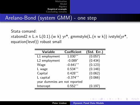
Arelano-Bond (system GMM) - one step
Stata comand:xtabond2 n L.n L(0.1).(w k) yr*, gmmstyle(L.(n w k)) ivstyle(yr*,equation(level)) robust small
Variable Coefficient (Std. Err.)
L1 employment 1.030∗∗ (0.057)L2 employment -0.089∗ (0.434)Wage -0.641∗∗ (0.123)L wage 0.534∗∗ (0.148)Capital 0.428∗∗ (0.062)L capital -0.374∗∗ (0.066)year dummies are not reportedIntercept 0.552∗∗ (0.197)
Peter Lindner Dynamic Panel Data Models

MotivationModel
AlgebraEmpirical example
Concluding remarks
Literature
Conclusions
How can we estimate a dynamic model with panel data
It is relatively complicated in theory but easy with stata
One has to carefully check the results from stata, because italways gives estimates.
Peter Lindner Dynamic Panel Data Models

MotivationModel
AlgebraEmpirical example
Concluding remarks
Literature
Literature
Econometric Analysis of Panel Data
Baltagi, Badi H., John Wiley & Sons, Ltd (2005); 3rd edition;especially Chapter 8
How to Do xtabond2: An Introduction to ”Difference” and”System” GMM in Stata
Roodman David, Center for Global Development, Working Paperno. 103, revised version 2001
Peter Lindner Dynamic Panel Data Models