Dynamic modelling of traction loads and renewable energy ...
217
i Dynamic modelling of traction loads and renewable energy systems on shared power lines for power quality assessment by Hein Naudé Thesis presented in fulfilment of the requirements for the degree Master of Engineering (Research) in the Faculty of Engineering at Stellenbosch University Supervisor: Dr. Johan Beukes Co-Supervisor: Dr. Ulrich Minnaar Department of Electrical & Electronic Engineering April 2019
Transcript of Dynamic modelling of traction loads and renewable energy ...

i
Dynamic modelling of traction loads and renewable energy
systems on shared power lines for power quality
assessment
by
Hein Naudé
Thesis presented in fulfilment of the requirements for the degree
Master of Engineering (Research) in the Faculty of Engineering
at Stellenbosch University
Supervisor: Dr. Johan Beukes
Co-Supervisor: Dr. Ulrich Minnaar
Department of Electrical & Electronic Engineering
April 2019

ii
Declaration
By submitting this thesis electronically I declare that the entirety of the work contained therein
is my own, original work, that I am the sole author thereof (save to the extent explicitly
otherwise stated), that reproduction and publication thereof by Stellenbosch University will not
infringe any third party rights and that I have not previously in its entirety or in part submitted it
for obtaining any qualification.
April 2019
H. Naudé
Copyright © 2019 Stellenbosch University All rights reserved
Stellenbosch University https://scholar.sun.ac.za

iii
Acknowledgements
I would like to thank my study leaders and mentors Dr. Johan Beukes and Dr. Ulrich Minnaar for allowing me to learn from their vast experience as engineers. Thank you for the continual support, advice and guidance during this project.
I would like to acknowledge the EPPEI Specialisation Centre in Renewable Energy and Power System Simulation for their financial support and contribution to this work.
I would like to thank my family in particular my parents, Hennie and Annerine Naudé, for their continual support during my student years and all the sacrifices that they have made for me to be able to do this work. I would not be in this position if not for them.
I would like to thank my close friends who made this road so much easier, including but not
restricted to: Hennie Louw, Armin Wagner, Jacques Wattel and Janke Jacobs.
Stellenbosch University https://scholar.sun.ac.za

iv
Abstract
Eskom has recently started investigating the effect of traction on renewable energy sources
due to the power quality problems associated with traction networks. Poor power quality
generated by means of traction networks have always been of concern. The impact of the
traction load power quality issues has greatly increased due to the increasing number of
renewable power producers (RPPs) being connected to the national grid. Studies has shown
an increase in voltage unbalance and harmonic distribution at various points of concern in the
network which leads to the loss of power production from the RPPs. Recent power quality
assessment reports from Eskom has indicated that power quality problems, particular
harmonic emissions, exist at RPPs. Harmonic sources such as non-linear (traction loads) are
contributors to voltage harmonic distortion on the network in addition to harmonic emissions of
RPPs.
To gain insight into the problem the need exist to model and simulate traction drive systems
and renewable power plants. DIgSILENT PowerFactory, was chosen as the software
simulation package to design and build generic models of renewable system inverters and
traction load rectifiers to conduct dynamic time domain simulations. To validate the accuracy
of the models, the simulation results were compared to measured results. Due to good
correlation, the models can be used for future network planning and power quality assessment.
The aim of this thesis is further to investigate the power quality issues related to traction loads
and to perform a power quality assessment at the POC of a local wind farm. The assessment
of voltage unbalance indicated that traction loads is generally the largest contributor to voltage
unbalance on a traction network and can cause inverter trips at RPPs at certain conditions. It
is observed that various conditions such as the traction load type, operating conditions and
control of the traction load, power demand of the traction loads and three-phase fault level will
impact the voltage unbalance caused by traction loads.
The impact of traction loads on the network voltage distortion is investigated and it is
determined that small current harmonics emissions of traction loads can generate large voltage
distortion at the presence of a parallel resonance. The impact of impedance and background
harmonics is investigated and the results show that the methods often described in standards
for calculating impedances to establish harmonic contribution will not always be valid,
especially when having inverters as harmonic sources.
A two-point measurement approach is followed for investigating the impact of traction load
current emissions on the assessment of RPP current emissions based on international
guidelines. A method is presented to approximate current emissions of the RPP without the
impact of the traction load current emissions on the assessment. The results show that traction
Stellenbosch University https://scholar.sun.ac.za

v
loads do impact the harmonic assessment of RPPs and therefore the current assessment
method will not always be accurate.
Stellenbosch University https://scholar.sun.ac.za

vi
Abstrak
Eskom het onlangs begin ondersoek wat die effek is van elektriese treinlaste op hernubare
energiebronne, weens die kragkwaliteitsprobleme wat verband hou met treinnetwerke. Swak
kragkwaliteit wat deur middel van treinnetwerke gegenereer word, was nog altyd ‘n probleem.
Die impak van die probleem het aansienlik toegeneem met die toename in die aantal
hernubare kragaanlegte wat gekoppel word aan die nasionale netwerk. Studies toon ‘n
toename in spanningswanbalans en harmoniek verspreiding op verskeie punte in die netwerk
wat lei tot die verlies van kragproduksie in hernubare kragaanlegte. ‘n Onlangse kragkwaliteit
assesseringsverslag in Eskom het aangedui dat kragkwaliteitsprobleme, veral harmoniese
emissies, by hernubare energiebronne bestaan. Nie-lineêre bronne soos treinlaste dra by tot
die harmoniese versteuring van spanning op die netwerk, asook harmoniese emissie van
hernubare kragaanlegte.
Om insig te verkry rakende die probleem, bestaan daar ‘n behoefte om treinstelsels en
hernubare kragaanlegte te modelleer. DIgSILENT PowerFactory, is gekies as die sagteware
simulasiepakket om generiese modelle van spanning wisselrigters in hernubare kragaanlegte
en spanning gelykrigters in treine te ontwerp en te bou om dinamiese tyddomein-simulasies te
doen. Die simulasie resultate is vergelyk met gemete resultate om die akkuraatheid van die
modelle te bevestig. Danksy goeie korrelasie tussen die simulasie resultate en gemete
resultate kan die modelle gebruik word vir toekomstige netwerkbeplanning en kragkwaliteit
assessering.
In hierdie studie word die kragkwaliteits probleme rakende elektriese treinlaste verder
ondersoek, asook die assessering van die kragkwaliteit by die punt van konneksie van 'n
plaaslike windplaas. Die assessering van die spanningswanbalans het aangedui dat elektriese
treinlaste hoofsaaklik die grootste bydrae lewer tot spanningswanbalans op treinnetwerke en
kan onder sekere omstandighede wisselrigter onderbrekings by hernubare kragaanlegte
veroorsaak. Daar word opgemerk dat verskillende toestande soos die tipe trein,
bedryfsomstandighede, beheer en drywingsaanvraag van die treinlas asook die driefase-
foutvlak die spanningswanbalans wat deur treinlaste veroorsaak word, sal beïnvloed.
Die impak van elektriese treine op die netwerkspanningvervorming is ondersoek en daar is
vasgestel dat die generasie van klein stroomharmonieke deur elektriese treinlaste groot
spanningsvervorming kan veroorsaak in die teenwoordigheid van parallelle resonansies. Die
impak van impedansie en agtergrond harmonieke is ondersoek en die resultate toon dat die
metodes wat in standaarde beskryf word om die impedansies te bereken vir die vasstelling
van die harmoniese bydrae, nie altyd geldig sal wees veral as wisselrigters as harmoniese
bronne voorkom nie.
Stellenbosch University https://scholar.sun.ac.za

vii
‘n Tweepunt metingsbenadering word gevolg om die impak van stroom harmonieke in
elektriese treinlaste op die assessering van stroom harmonieke in hernubare kragaanlegte te
ondersoek. ‘n Metode word aangebied om die stroom harmonieke van hernubare kragaanlegte
te benader sonder die impak van elektriese treinlaste op die assessering. Die resultate toon
dat die harmoniese stroom van elektriese treinlaste wel die assessering van stroom
harmonieke in hernubare kragaanlegte beïnvloed en dat die huidige asseseringsmetode dus
nie altyd akkuraat sal wees nie.
Stellenbosch University https://scholar.sun.ac.za

viii
Contents
DECLARATION .................................................................................................................................................. II
ACKNOWLEDGEMENTS ................................................................................................................................... III
ABSTRACT ....................................................................................................................................................... IV
ABSTRAK ......................................................................................................................................................... VI
CONTENTS ..................................................................................................................................................... VIII
LIST OF TABLES .............................................................................................................................................. XIII
LIST OF FIGURES ............................................................................................................................................ XIV
LIST OF ACRONYMS AND ABBREVIATIONS .................................................................................................... XXI
CHAPTER 1 INTRODUCTION .............................................................................................................................. 1
1.1. PROJECT BACKGROUND ............................................................................................................................. 1
1.2. OVERVIEW OF THE TRACTION NETWORK IN SOUTH AFRICA .................................................................... 2
1.3. OVERVIEW OF TRACTION SUBSTATIONS IN SOUTH AFRICA ...................................................................... 3
1.4. OBJECTIVE .................................................................................................................................................. 8
1.5. RESEARCH QUESTIONS ............................................................................................................................... 8
1.6. THESIS STRUCTURE .................................................................................................................................... 8
CHAPTER 2 LITERATURE REVIEW .................................................................................................................... 10
2.1. INTRODUCTION ........................................................................................................................................ 10
2.2. OVERVIEW OF TRACTION LOADS IN SOUTH AFRICA ................................................................................ 10
2.2.1. Single-phase active rectifier locomotives ............................................................................................ 11
2.2.2. Single-phase half-controlled rectifier locomotives .............................................................................. 13
2.3. DYNAMIC NATURE OF TRACTION LOADS ................................................................................................. 14
2.3.1. Mathematical model ........................................................................................................................... 15
2.4. INVERTERS IN RENEWABLE ENERGY SYSTEMS ........................................................................................ 20
2.4.1. Overview on inverter topologies ......................................................................................................... 20
2.4.2. Overview on sinusoidal based PWM scheme ...................................................................................... 22
2.4.3. Output filters for grid-connected inverters ......................................................................................... 23
2.4.4. Sampling .............................................................................................................................................. 24
2.4.4.1. Naturally sampled PWM ............................................................................................................. 24
2.4.4.2. Regularly sampled PWM ............................................................................................................. 24
2.4.4.3. Direct modulation ....................................................................................................................... 25
2.4.5. Third harmonic injection ..................................................................................................................... 25
2.4.6. Overview on space vector based PWM scheme .................................................................................. 25
2.4.7. Inverter control techniques ................................................................................................................. 26
2.5. PQ STANDARD IN SOUTH AFRICA ............................................................................................................ 27
Stellenbosch University https://scholar.sun.ac.za

ix
2.5.1. Overview .............................................................................................................................................. 27
2.5.2. PQ standards in renewable energy ...................................................................................................... 27
2.5.2.1. Design and operation requirements of RPPs............................................................................... 27
2.5.2.2. PQ parameters of RPPs ............................................................................................................... 28
2.5.3. PQ measurement standards ................................................................................................................ 28
2.5.3.1. Measurement instrument classes ............................................................................................... 29
2.5.3.2. Data aggregation ........................................................................................................................ 29
2.5.3.3. Flagging due to dips, swells or interruptions .............................................................................. 30
2.6. PQ MANAGEMENT AND ASSESSMENT IN SOUTH AFRICA ....................................................................... 30
2.6.1. Overview .............................................................................................................................................. 30
2.6.2. Assessment requirements ................................................................................................................... 30
2.6.3. Voltage Unbalance ............................................................................................................................... 31
2.6.3.1. Compatibility levels ..................................................................................................................... 31
2.6.3.2. Planning levels ............................................................................................................................ 31
2.6.3.3. Calculation of unbalance emissions ............................................................................................ 31
2.6.3.4. Calculation of unbalance emissions of RPP for compliance assessment ..................................... 32
2.6.4. Harmonics ............................................................................................................................................ 32
2.6.4.1. Voltage harmonic compatibility levels ........................................................................................ 32
2.6.4.2. Voltage harmonic planning levels ............................................................................................... 33
2.6.4.3. Calculation of harmonic emissions of RPP for compliance assessment ...................................... 34
2.6.4.4. Current harmonic emission levels ............................................................................................... 37
2.7. PQ IMPACT OF AC TRACTION ON NETWORK ........................................................................................... 38
2.7.1. Introduction ......................................................................................................................................... 38
2.7.2. Voltage Unbalance ............................................................................................................................... 38
2.7.3. Harmonics ............................................................................................................................................ 39
2.7.4. System resonance ................................................................................................................................ 40
2.7.4.1. Overview ..................................................................................................................................... 40
2.7.4.2. Parallel resonance ....................................................................................................................... 41
2.7.4.3. Series resonance ......................................................................................................................... 43
2.7.5. Voltage fluctuations ............................................................................................................................. 44
2.8. MITIGATION METHODS TO REDUCE POOR PQ IN TRACTION NETWORKS............................................... 46
2.8.1. Phase-shift method ............................................................................................................................. 47
2.8.2. Self-balancing traction transformers ................................................................................................... 47
2.8.3. Passive filter and reactive power compensation ................................................................................. 49
2.8.4. Dynamic compensation methods ........................................................................................................ 49
2.9. CONCLUSION ............................................................................................................................................ 52
CHAPTER 3 SIMULATION MODELS .................................................................................................................. 53
3.1. INTRODUCTION ........................................................................................................................................ 53
3.2. OVERVIEW ON DIGSILENT POWERFACTORY ............................................................................................ 55
Stellenbosch University https://scholar.sun.ac.za

x
3.2.1. DIgSILENT PowerFactory limitations ................................................................................................... 56
3.2.2. RMS and EMT simulations ................................................................................................................... 56
3.3. DIGSILENT POWERFACTORY BUILT-IN MODELS ....................................................................................... 57
3.3.1. PWM converter model ........................................................................................................................ 57
3.3.1.1. Modelling of PWM inverter losses .............................................................................................. 58
3.3.1.2. Load flow control conditions of PWM converter......................................................................... 58
3.3.1.3. RMS and EMT control of PWM converter – controlled voltage source model ............................ 59
3.3.1.4. RMS and EMT control of PWM converter – detailed model ....................................................... 60
3.3.1.5. PWM converter model limitations .............................................................................................. 61
3.3.2. AC and DC cables ................................................................................................................................. 61
3.3.3. Built-in PLL model ................................................................................................................................ 61
3.3.4. Built-in sample and hold element........................................................................................................ 61
3.3.5. Built-in voltage measurement element ............................................................................................... 61
3.3.6. Built-in current measurement element ............................................................................................... 62
3.3.7. Built-in power measurement element ................................................................................................ 62
3.4. CONTROL OF CONVERTER - POWER FLOW THEORY ................................................................................ 62
3.5. TRACTION LOAD (RECTIFIER) MODELLING ............................................................................................... 66
3.5.1. DIgSILENT PowerFactory active rectifier model .................................................................................. 66
3.5.1.1. Overview ..................................................................................................................................... 66
3.5.1.2. Element layout in DIgSILENT PowerFactory ................................................................................ 68
3.5.1.3. Composite model in DIgSILENT PowerFactory ............................................................................ 68
3.5.1.4. DSL model of voltage controller in DIgSILENT PowerFactory ...................................................... 70
3.5.1.5. DSL model of current controller in DIgSILENT PowerFactory ...................................................... 70
3.5.1.6. Working principle of an active rectifier in DIgSILENT PowerFactory ........................................... 71
3.5.2. DIgSILENT PowerFactory half-controlled thyristor rectifier model ..................................................... 74
3.5.2.1. Overview ..................................................................................................................................... 74
3.5.2.2. Element layout in DIgSILENT PowerFactory ................................................................................ 75
3.5.2.3. Composite model in DIgSILENT PowerFactory ............................................................................ 76
3.5.2.4. DSL model of pulse generator in DIgSILENT PowerFactory ......................................................... 77
3.5.2.5. Working principle of a half-controlled thyristor rectifier in DIgSILENT PowerFactory ................ 77
3.6. WIND FARM (INVERTER) MODELLING ..................................................................................................... 78
3.6.1. Inverter hardware – Wind farm A ....................................................................................................... 78
3.6.2. Inverter hardware – Wind farm B ........................................................................................................ 79
3.6.3. DIgSILENT PowerFactory hysteresis inverter model – Wind farm A ................................................... 79
3.6.3.1. Overview ..................................................................................................................................... 79
3.6.3.2. Element layout in DIgSILENT PowerFactory ................................................................................ 83
3.6.3.3. Hysteresis inverter composite model .......................................................................................... 84
3.6.3.4. Voltage controller ....................................................................................................................... 85
3.6.3.5. Current controller ........................................................................................................................ 85
Stellenbosch University https://scholar.sun.ac.za

xi
3.6.3.6. Working principle of a three-phase hysteresis inverter in DIgSILENT PowerFactory .................. 86
3.6.4. DIgSILENT PowerFactory conventional PWM inverter model – Wind farm B ..................................... 88
3.6.4.1. Overview ..................................................................................................................................... 88
3.6.4.2. Element layout in DIgSILENT PowerFactory ................................................................................ 89
3.6.4.3. PWM inverter composite model ................................................................................................. 90
3.6.4.4. Power controller (labelled as PC in Figure 68) ............................................................................ 92
3.6.4.5. Current controller ........................................................................................................................ 95
3.6.5. DIgSILENT PowerFactory interleaved PWM inverter model – Wind farm B (revised) ....................... 100
3.6.5.1. Overview ................................................................................................................................... 100
3.6.5.2. Element layout in DIgSILENT PowerFactory .............................................................................. 101
3.6.5.3. Composite model of a single three-phase PWM inverter ......................................................... 102
3.7. CONCLUSION .......................................................................................................................................... 103
CHAPTER 4 THE IMPACT OF WIND FARMS ON NETWORK HARMONICS ....................................................... 105
4.1. INTRODUCTION ...................................................................................................................................... 105
4.2. MEASURMENT SETUP AT WIND FARMS ................................................................................................ 105
4.3. WIND FARM A – HYSTERESIS INVERTER................................................................................................. 107
4.3.1. Measurement results – Oscilloscope ................................................................................................. 107
4.3.2. Measurement results – Elspec .......................................................................................................... 109
4.3.2.1. One-cycle window harmonics ................................................................................................... 109
4.3.2.2. 3-second window harmonics .................................................................................................... 112
4.3.2.3. 10-minute window harmonics .................................................................................................. 114
4.3.3. Simulation results - Wind farm A ....................................................................................................... 116
4.3.3.1. Parallel resonance ..................................................................................................................... 116
4.3.3.2. Waveform and harmonic analysis ............................................................................................ 117
4.3.4. Comparison of measurement and simulation results - Wind farm A ................................................ 118
4.4. WIND FARM B – PWM INVERTER ........................................................................................................... 119
4.4.1. Measurement results – Oscilloscope ................................................................................................. 119
4.4.2. Measurement results – Elspec........................................................................................................... 120
4.4.3. Simulation results – Wind farm B ...................................................................................................... 124
4.4.4. Comparison of measurement and simulation results ....................................................................... 127
4.5. CONCLUSION .......................................................................................................................................... 128
CHAPTER 5 THE IMPACT OF TRACTION LOADS ON NETWORK VOLTAGE UNBALANCE .................................. 129
5.1. INTRODUCTION ...................................................................................................................................... 129
5.2. MEASUREMENT INSTALLATION AND SETUP .......................................................................................... 129
5.3. VOLTAGE UNBALANCE EMMISIONS BY WIND FARM A ......................................................................... 132
5.4. MEASUREMENT RESULTS ....................................................................................................................... 133
5.4.1. Weekly (long term) PQ assessment ................................................................................................... 133
5.4.1.1. Voltage unbalance .................................................................................................................... 133
Stellenbosch University https://scholar.sun.ac.za

xii
5.4.1.2. Voltage fluctuations .................................................................................................................. 133
5.4.2. Worst case (short term) PQ assessment ........................................................................................... 134
5.4.2.1. Voltage unbalance .................................................................................................................... 134
5.5. SIMULATION SETUP ............................................................................................................................... 137
5.6. SIMULATION RESULTS ............................................................................................................................ 138
5.7. THE EFFECT OF VOLTAGE UNBALANCE ON WIND FARM ....................................................................... 140
5.8. CONCLUSION .......................................................................................................................................... 142
CHAPTER 6 THE IMPACT OF TRACTION LOADS ON NETWORK HARMONICS ................................................. 143
6.1. INTRODUCTION ...................................................................................................................................... 143
6.2. MEASUREMENT SETUP .......................................................................................................................... 143
6.3. VOLTAGE THD ASSESSMENT (WEEKLY (LONG-TERM) ASSESSMENT) .................................................... 143
6.4. VOLTAGE THD ASSESSMENT (SHORT-TERM) ......................................................................................... 144
6.5. INDIVIDUAL VOLTAGE HARMONIC ASSESSMENT (WEEKLY (LONG-TERM) ASSESSMENT) .................... 147
6.6. MEASURED LOCOMOTIVE INDIVIDUAL HARMONIC EMISSIONS ........................................................... 155
6.6.1. Half-controlled thyristor rectifiers ..................................................................................................... 156
6.6.2. Active rectifiers .................................................................................................................................. 162
6.7. SIMULATED INDIVIDUAL HARMONIC EMISSIONS .................................................................................. 165
6.7.1. Half-controlled thyristor rectifier ...................................................................................................... 165
6.7.2. Active rectifier ................................................................................................................................... 166
6.8. THE IMPACT OF IMPEDANCE AND BACKGROUND HARMONICS ON EMISSION LEVELS OF RPP ............ 168
6.9. CONCLUSION .......................................................................................................................................... 178
CHAPTER 7 CONCLUSION ............................................................................................................................. 179
7.1. SYNOPSIS ................................................................................................................................................ 179
7.2. FUTURE WORK ....................................................................................................................................... 181
REFERENCES ................................................................................................................................................. 182
APPENDIX..................................................................................................................................................... 193
Stellenbosch University https://scholar.sun.ac.za

xiii
List of tables
Table 1: RPP categories [37] ................................................................................................28
Table 2: Compatibility levels for voltage harmonics on HV networks [5] ...............................33
Table 3: Planning levels for voltage harmonics on HV networks [38] ....................................33
Table 4: Inverter trip settings .............................................................................................. 140
Table 5: The measured 95th percentile THD voltages of phase A, B and C ........................ 144
Table 6: The 95th percentile measured three-phase voltage harmonic that exceeded the NRS
048-2 limits ......................................................................................................................... 149
Table 7: Individual current harmonic emission levels .......................................................... 174
Table 8: Results from investigation ..................................................................................... 174
Stellenbosch University https://scholar.sun.ac.za

xiv
List of figures
Figure 1: Network geographical diagram ............................................................................... 3
Figure 2: Conventional 25 kV AC traction substation diagram ............................................... 4
Figure 3: Traction substation with one transformer ................................................................ 5
Figure 4: Connection between catenary and traction substation with one transformer ........... 5
Figure 5: 25 kV AC traction substation diagram with two transformers .................................. 6
Figure 6: Traction substation with two transformers ............................................................... 6
Figure 7: Connection between catenary and traction substation with two transformers ......... 7
Figure 8: Neutral section ....................................................................................................... 7
Figure 9: Traction drive system ............................................................................................12
Figure 10: Conventional half-controlled thyristor traction system ..........................................13
Figure 11: Velocity curve of a locomotive .............................................................................15
Figure 12: Traction effort curve of a locomotive ....................................................................16
Figure 13: Power consumption curve of a locomotive ...........................................................16
Figure 14: Forces on a locomotive .......................................................................................17
Figure 15: Simplified velocity curve of a locomotive ..............................................................18
Figure 16: Acceleration and deceleration curve of a locomotive ...........................................19
Figure 17: Locomotive displacement curve ...........................................................................19
Figure 18: Type of inverters: (a) VSI (b) CSI .........................................................................21
Figure 19: Three-phase VSI equivalent circuit ......................................................................22
Figure 20: Pulse width modulation ........................................................................................22
Figure 21: Illustration of SVM ...............................................................................................26
Figure 22: Superposition of harmonic sources ......................................................................35
Figure 23: Harmonic impedance representation ...................................................................37
Figure 24: Parallel resonance between line impedance and customer load impedance........41
Figure 25: Frequency sweep of parallel resonance network .................................................42
Figure 26: Series resonance circuit ......................................................................................43
Figure 27: Frequency sweep of series resonance network ...................................................44
Figure 28: Single-phase voltage dip characteristics ..............................................................45
Figure 29: VRTC for category C RPPs [37] ..........................................................................45
Figure 30: Reactive power support requirements for RPPs [37] ...........................................46
Figure 31: Traction power supply system with V/v traction transformer ................................47
Figure 32: Traction power supply system with Scott traction transformer .............................48
Figure 33: Traction power supply system with conventional SVC .........................................50
Figure 34: Traction power supply system with RPC ..............................................................51
Figure 35: PWM converter model with series reactance, no-load losses and load losses .....57
Figure 36: Block diagram of the built-in current controller in the PWM controller model ........60
Stellenbosch University https://scholar.sun.ac.za

xv
Figure 37: Power flow between two voltage sources ............................................................63
Figure 38: Voltage and current phasor diagram for inverter mode of operation ....................64
Figure 39: Voltage and current phasor diagram for rectifier mode of operation .....................65
Figure 40: Active and reactive power magnitude as a function of δ .....................................66
Figure 41: Active and reactive power magnitude as a function of δ around operating point of
0.1489 radδ = − ...................................................................................................................67
Figure 42: Designed control layout of a single-phase active rectifier.....................................67
Figure 43: Network diagram of the single-phase active rectifier traction system ...................68
Figure 44: Designed composite model of the single-phase active rectifier in PowerFactory .69
Figure 45: Designed active rectifier voltage controller DSL model in DIgSILENT PowerFactory
.............................................................................................................................................70
Figure 46: Designed active rectifier current controller DSL model in DIgSILENT PowerFactory
.............................................................................................................................................71
Figure 47: PWM generator reference and triangle signal ......................................................72
Figure 48: PWM generator reference and phase A switching signal .....................................72
Figure 49: Inverter current waveform ....................................................................................73
Figure 50: Grid voltage waveform .........................................................................................73
Figure 51: Inverter AC power waveform ...............................................................................74
Figure 52: Simplified model of traction drive .........................................................................75
Figure 53: Network diagram of single-phase half-controlled thyristor controlled system in
DIgSILENT PowerFactory ....................................................................................................76
Figure 54: Designed composite model of half-controlled thyristor rectifier in DIgSILENT
PowerFactory .......................................................................................................................76
Figure 55: Designed pulse generator DSL model in DIgSILENT PowerFactory ....................77
Figure 56: AC voltage waveform and thyristor gate signals ..................................................78
Figure 57: Conventional hysteresis current controller ...........................................................80
Figure 58: Conventional hysteresis current control switching diagram ..................................81
Figure 59: Network diagram of hysteresis wind farm system in DIgSILENT PowerFactory ...83
Figure 60: Designed composite model of hysteresis inverter model in DIgSILENT
PowerFactory .......................................................................................................................84
Figure 61: Hysteresis inverter voltage controller in DIgSILENT PowerFactory ......................85
Figure 62: Hysteresis inverter current controller in DIgSILENT PowerFactory ......................86
Figure 63: Measured inverter output phase A current (red) and reference current (black) ....87
Figure 64: Inverter output measured phase A current compared to the hysteresis band.......87
Figure 65: Single-line equivalent circuit of three-phase grid-connected VSI..........................88
Figure 66: Designed control layout of grid-connected VSI ....................................................89
Figure 67: Network diagram of PWM wind farm system in DIgSILENT PowerFactory ..........90
Figure 68: Composite model of PWM inverter model in DIgSILENT PowerFactory ..............91
Stellenbosch University https://scholar.sun.ac.za

xvi
Figure 69: Power control loop block diagram ........................................................................92
Figure 70: Closed loop active and reactive power controller .................................................94
Figure 71: Designed inverter power controller for PWM inverter in DIgSILENT PowerFactory
.............................................................................................................................................95
Figure 72: Inverter control block diagram in the frequency domain with feedforward of grid
voltage and current to cancel their effect on output ..............................................................97
Figure 73: Reduced model of inverter control block diagram in the frequency domain with
feedforward of grid voltage and current to cancel their effect on output ................................97
Figure 74: Root locus plot of the current controller ...............................................................99
Figure 75: Current controller block diagram in DIgSILENT PowerFactory........................... 100
Figure 76: Single-line diagram of interleaved inverter connected to grid ............................. 101
Figure 77: Network diagram of interleaved PWM inverter in DIgSILENT PowerFactory...... 102
Figure 78: Composite model of PWM inverter in DIgSILENT PowerFactory ....................... 103
Figure 79: Single-line diagram of the wind farm installation ................................................ 106
Figure 80: Three-phase delta 3 wire Elspec connection diagram ........................................ 107
Figure 81: Inverter phase voltage (blue) and phase voltage harmonic spectrum (red) (snapshot
1) measured by oscilloscope .............................................................................................. 108
Figure 82: Inverter phase voltage waveform (blue), current waveforms (cyan) and phase
current harmonic spectrum (red) (snapshot 2) measured by oscilloscope .......................... 109
Figure 83: Inverter phase current waveform recorded by Elspec ........................................ 110
Figure 84: Harmonic spectrum of inverter phase current recorded by Elspec for one-cycle
window ............................................................................................................................... 110
Figure 85: Inverter phase voltage waveform recorded by Elspec ........................................ 111
Figure 86: Harmonic spectrum of inverter phase voltage recorded by Elspec for one-cycle
window ............................................................................................................................... 111
Figure 87: Harmonic spectrum of inverter phase voltage recorded by Elspec for one-cycle
window (detailed) ............................................................................................................... 112
Figure 88: Harmonic spectrum of inverter phase current recorded by Elspec for 3-second
window ............................................................................................................................... 113
Figure 89: Harmonic spectrum of inverter phase voltage recorded by Elspec for 3-second
window ............................................................................................................................... 113
Figure 90: Harmonic spectrum of inverter phase voltage recorded by Elspec for 3-second
window (detailed) ............................................................................................................... 114
Figure 91: Harmonic spectrum of inverter phase current recorded by Elspec for 10-minute
window ............................................................................................................................... 114
Figure 92: Harmonic spectrum of inverter phase voltage recorded by Elspec for 10-minute
window ............................................................................................................................... 115
Stellenbosch University https://scholar.sun.ac.za

xvii
Figure 93: Harmonic spectrum of inverter phase voltage recorded by Elspec for 10-minute
window (detailed) ............................................................................................................... 115
Figure 94: Network impedance at 0.69 kV terminal ............................................................ 116
Figure 95: Network impedance at 132 kV terminal ............................................................. 117
Figure 96: Hysteresis inverter phase current waveform in DIgSILENT PowerFactory ......... 117
Figure 97: Grid phase current waveform in DIgSILENT PowerFactory ............................... 118
Figure 98: Harmonic spectrum the grid phase current in DIgSILENT PowerFactory ........... 118
Figure 99: Inverter phase voltage waveform (blue), current waveform (cyan) and phase current
harmonic spectrum (red) (snapshot 1) measured by oscilloscope ...................................... 119
Figure 100: Inverter phase voltage waveform (blue), current waveform (cyan) and phase
current harmonic spectrum (red) (snapshot 2) measured by oscilloscope .......................... 120
Figure 101: Inverter phase voltage recorded by Elspec (detailed) for one cycle ................. 121
Figure 102: Harmonic spectrum of inverter phase voltage as a percentage of the fundamental
voltage recorded by Elspec ................................................................................................ 121
Figure 103: Harmonic spectrum of inverter phase voltage as a percentage of the fundamental
voltage recorded by Elspec (detailed) ................................................................................. 122
Figure 104: Inverter phase current recorded by Elspec (detailed) for 1 cycle ...................... 123
Figure 105: Harmonic spectrum of inverter phase current as a percentage of the fundamental
current recorded by Elspec ................................................................................................. 123
Figure 106: Harmonic spectrum of inverter phase current as a percentage of the fundamental
current recorded by Elspec (detailed) ................................................................................. 124
Figure 107: Phase current of each individual inverter module in DIgSILENT PowerFactory
........................................................................................................................................... 125
Figure 108: Harmonic spectrum of the phase current as percentage of fundamental current of
each individual inverter module in DIgSILENT PowerFactory ............................................. 125
Figure 109: Phase currents of the three individual inverter modules in DIgSILENT Powerfactory
........................................................................................................................................... 126
Figure 110: Phase current of interleaved inverter in DIgSILENT PowerFactory .................. 126
Figure 111: Harmonic spectrum the phase current of the interleaved inverter in DIgSILENT
PowerFactory ..................................................................................................................... 127
Figure 112: Single-line network diagram with the locations of the Elspec installations ........ 130
Figure 113: Single-phase Elspec connection diagram ........................................................ 131
Figure 114: Three-phase delta 3 wire Elspec connection diagram ...................................... 131
Figure 115: Physical voltage clamps connections............................................................... 132
Figure 116: Physical current probes connections ............................................................... 132
Figure 117: Voltage dip events ........................................................................................... 134
Figure 118: 10-minute negative sequence voltage unbalance at Wind farm A .................... 135
Figure 119: RMS phase current at traction substation ........................................................ 135
Stellenbosch University https://scholar.sun.ac.za

xviii
Figure 120: Measured negative sequence unbalance at Wind farm A ................................ 136
Figure 121: RMS phase voltages of phase A (a), phase B (b) and phase C (c) at Wind farm A
........................................................................................................................................... 137
Figure 122: High level network diagram in DIgSILENT PowerFactory ................................ 138
Figure 123: Simulated negative sequence unbalance ........................................................ 139
Figure 124: Simulated RMS phase voltages at the 0.69 kV terminal .................................. 139
Figure 125: Measured RMS phase voltages at Wind farm A .............................................. 140
Figure 126: The upper (blue) and lower (red) voltage limits for a wind turbine inverter ....... 141
Figure 127: The upper (blue) and lower (red) voltage limits for a wind turbine inverter ....... 141
Figure 128: Measured 10-minute voltage THD of phase A (a), phase B (b) and phase C (c) at
Wind farm A ....................................................................................................................... 145
Figure 129: Measured instantaneous voltage THD of phase A (a), phase B (b) and phase C
(c) at Wind farm A .............................................................................................................. 146
Figure 130: The maximum measured voltage harmonic content of phase A (red), phase B
(green) and phase C (blue) ................................................................................................ 147
Figure 131: The 95th percentile measured voltage harmonic content of phase A (red) compared
to the corresponding harmonic limit (black) ........................................................................ 148
Figure 132: The 95th percentile measured voltage harmonic content of phase B (green)
compared to the corresponding harmonic limit (black) ........................................................ 148
Figure 133: The 95th percentile measured voltage harmonic content of phase C (blue)
compared to the corresponding harmonic limit (black) ........................................................ 149
Figure 134: Measured 10-minute aggregated 3rd voltage harmonic at POC........................ 150
Figure 135: Measured 10-minute aggregated 5th voltage harmonic at POC ........................ 151
Figure 136: Measured 10-minute aggregated 7th voltage harmonic at POC ........................ 152
Figure 137: Measured 10-minute aggregated 39th voltage harmonic at POC ...................... 153
Figure 138: Simulated parallel resonance at POC .............................................................. 153
Figure 139: Measured 10-minute aggregated 39th current harmonic at POC ...................... 154
Figure 140: Measured 10-minute aggregated 43rd voltage harmonic at POC ...................... 155
Figure 141: Measured 10-minute aggregated 43rd current harmonic at POC ...................... 155
Figure 142: Measured single-phase current waveform on 132 kV side of traction substation
transformer (snapshot 1) .................................................................................................... 156
Figure 143: Measured current harmonics as a percentage of the fundamental current
magnitude on 132 kV side of traction substation transformer (snapshot 1) ......................... 157
Figure 144: Measured phase voltage waveform on 132 kV side of traction substation
transformer (snapshot 1) .................................................................................................... 157
Figure 145: Measured voltage harmonics as a percentage of the fundamental voltage
magnitude on 132 kV side of traction substation transformer (snapshot 1) ......................... 158
Stellenbosch University https://scholar.sun.ac.za

xix
Figure 146: Measured single-phase current waveform on 132 kV side of traction substation
transformer (snapshot 2) .................................................................................................... 158
Figure 147: Measured phase voltage waveform on 132 kV side of traction substation
transformer (snapshot 2) .................................................................................................... 159
Figure 148: Measured current harmonics as a percentage of the fundamental current
magnitude on 132 kV side of traction substation transformer (snapshot 2) ......................... 159
Figure 149: Measured voltage harmonics as a percentage of the fundamental voltage
magnitude on 132 kV side of traction substation transformer (snapshot 2) ......................... 160
Figure 150: Measured single-phase current waveform on 132 kV side of traction substation
transformer (snapshot 3) .................................................................................................... 160
Figure 151: Measured phase voltage waveform on 132 kV side of traction substation
transformer (snapshot 3) .................................................................................................... 161
Figure 152: Measured current harmonics as a percentage of the fundamental current
magnitude on 132 kV side of traction substation transformer (snapshot 3) ......................... 161
Figure 153: Measured voltage harmonics as a percentage of the fundamental voltage
magnitude on 132 kV side of traction substation transformer (snapshot 3) ......................... 162
Figure 154: Measured single-phase current waveform on 132 kV side of traction substation
transformer (snapshot 4) .................................................................................................... 163
Figure 155: Measured phase voltage waveform on 132 kV side of traction substation
transformer (snapshot 4) .................................................................................................... 163
Figure 156: Measured current harmonics as a percentage of the fundamental current
magnitude on 132 kV side of traction substation transformer (snapshot 4) ......................... 164
Figure 157: Measured voltage harmonics as a percentage of the fundamental voltage
magnitude on 132 kV side of traction substation transformer (snapshot 4) ......................... 164
Figure 158: Simulated single-phase current waveform on 132 kV side of traction substation
transformer ......................................................................................................................... 165
Figure 159: Simulated current harmonics as a percentage of the fundamental current
magnitude on 132 kV side of traction substation transformer ............................................. 166
Figure 160: Simulated parallel resonance in traction system .............................................. 166
Figure 161: Simulated single-phase current waveform on 132 kV side of traction substation
transformer ......................................................................................................................... 167
Figure 162: Simulated current harmonics as a percentage of the fundamental current
magnitude on 132 kV side of traction substation transformer ............................................. 167
Figure 163: Simulink model of inverters connected to a simple LV feeder .......................... 169
Figure 164: Harmonic spectrum of voltage at installation 1 without background harmonics ‘o’
and with third order background harmonic ‘x’ ..................................................................... 170
Figure 165: Harmonic spectrum of voltage at installation 1 with third order background
harmonic and 1 nF filter capacitance ‘o’ and 1 Fµ filter capacitance ‘x’ .............................. 171
Stellenbosch University https://scholar.sun.ac.za

xx
Figure 166: Harmonic spectrum of voltage at installation 1 with 2 kHz background harmonic
and 1 nF filter capacitance ‘o’ and 1 Fµ filter capacitance ‘x’ .............................................. 171
Figure 167: Impedance plots pZ for 1nFfC = and 1 FfC µ= and hZ and 3hZ × ............ 173
Figure 168: Measured 10-minute aggregated 31st current harmonic at traction substation . 176
Figure 169: Measured 10-minute aggregated 31st current harmonic at POC ...................... 176
Figure 170: Measured instantaneous 31st current harmonic at the POC ............................. 177
Figure 171: Detailed traction layout diagram ...................................................................... 193
Figure 172: ABB inverter module drawing .......................................................................... 194
Figure 173: Nameplate of the ABB inverter module ............................................................ 194
Figure 174: Nameplate of traction transformer ................................................................... 195
Stellenbosch University https://scholar.sun.ac.za

xxi
List of acronyms and abbreviations
AC Alternating Current
APQC Active Power Quality Compensator
CSI Current Source Inverter
CT Current Transformer
DC Direct Current
DCUOSA Distribution Connection and Use-of-System Agreement with Generators
DSL Dynamic Simulation Language
EHV Extra High Voltage
EMT Electro-Magnetic Transient
HV High Voltage
HVDC High Voltage Direct Current
IGBT Insulated-Gate Bipolar Transistor
LV Low Voltage
MV Medium Voltage
PI Proportional Integral
PLL Phase-Locked Loop
POC Point of Connection
PQ Power Quality
PV Photovoltaic
PWM Pulse Width Modulated
RMS Root Means Square
RPC Railway Power Static Conditioner
RPP Renewable Power Plant
SAGCRPP South Africa Grid Code for Renewable Power Plants
STATCOM Static Synchronous Compensator
SVC Static VAr Compensator
SVM Space Vector Modulation
VRTC Voltage Ride Through Conditions
Stellenbosch University https://scholar.sun.ac.za

xxii
VSC Voltage Source Converter
VSI Voltage Source Inverter
VT Voltage Transformer
Stellenbosch University https://scholar.sun.ac.za

1
CHAPTER 1
INTRODUCTION
1.1. PROJECT BACKGROUND
The introduction of renewable power plants (RPPs) on traction/railway networks has
introduced power quality (PQ) problems in South Africa. Therefore, it has recently become
importance to investigate the effect of traction loads on renewable energy sources, particularly
solar photovoltaic (PV) and wind. Traction loads are typically locomotives with multiple power
units that are used to move a large load such as freight or passenger vehicles. Poor PQ
generated by means of traction networks has always been of concern. The impact of this
concern has greatly increased due to the increasing number of RPPs being connected to the
national grid, as it presents a new dimension to traction/railway network PQ concerns. Recent
reports from Eskom has shown an increase in voltage unbalance and harmonic distribution at
various points of concern in the network which leads to the loss of power production from the
RPPs [1]. A particular Eskom report claimed for unfavourable network conditions which in turn
prevented maximum power production and exportation to the grid [2]. This may be due to an
unbalanced supply caused by large single-phase loads within a traction network or a
disconnection of inverters caused by harmonics generated in traction loads.
Traction loads are dynamic and depend on a number of parameters that need to be considered
such as the mass, traction effort and speed of the train [3], [4]. Current network simulations
being done in Eskom assumes a constant traction load and consequently require an updated
traction load simulation model to provide a more accurate simulation analysis in time domain.
The existing measurement framework as required by local standards e.g. NRS048-2 [5] does
not make provision for the short-term dynamic PQ changes and needs to be investigated as
short-term dynamic behaviour of traction loads will influence RPPs. It is important to ensure
high quality of power at all times as this problem will only increase due to legislation and supply
constraints to add as much renewable generation capacity as possible.
The aim of the project is to investigate the impact of traction networks on RPPs with the focus
on wind power generation. Therefore, a detailed research study will be done on the PQ
problems introduced by 25 kV alternating current (AC) traction networks. Various PQ problems
such as voltage unbalance, harmonics, parallel resonance effect and low-frequency voltage
fluctuations have drawn more attention in recent years due to their adverse effect on traction
network devices and utility grids thus leading to a detailed study of these issues [6]. To
investigate PQ in a power system it becomes important to understand the different non-linear
loads and sources within a network.
Stellenbosch University https://scholar.sun.ac.za

2
Therefore, the time domain modelling of AC traction load simulation models will be studied
utilizing DIgSILENT PowerFactory software and an embedded application of either Python or
DIgSILENT programming language. Different wind farm inverter topologies will be studied
using measurement data and the simulation of time domain DIgSILENT PowerFactory models.
The network load and generation change dynamically due to the dynamic nature of traction
loads and inverters. Therefore, inverters will trip on instantaneous ratings. An average
frequency analysis approach is not sufficient in describing the PQ issues in a dynamic network.
Consequently, a time domain approach is required to accurately describe PQ issues on a
dynamic network. Two local wind farms will be used as case studies for the investigation. The
South African grid code for renewable power plants (SAGCRPP) to which every RPP must
adhere to obtain compliance as well as the IEC 61000-4-30 which determines how PQ is
measured will be investigated to develop guidelines to minimize the impact of traction loads
on renewable energy generation.
1.2. OVERVIEW OF THE TRACTION NETWORK IN SOUTH AFRICA
The network on which this research study is based is located in the Northern Cape Province
and Eastern Cape Province of South Africa between Cradock and De Aar. Refer to Figure 1
for the network overhead geographical diagram as obtained from DIgSILENT PowerFactory.
The 132 kV line is mainly used as a traction line that contain RPPs in the form of a wind farm
(Wind farm A) and a solar PV plant (Solar PV). The encircled dots show the traction substations
along the 132 kV line. This makes this particular network a useful case study as the PQ impact
of traction can be studied on both wind and solar PV generation. A recent quality of supply
report at Wind farm A has indicated that PQ problems, particular harmonic emissions, exist at
the RPP, therefore making this study relative to the present problem at the RPP. The quality
of supply report also indicated a change in power flow direction when the RPP reached a
certain power generation which could contribute to the PQ problems present. Therefore, it is
clear that a number of issues are at play in this network. Refer to Figure 171 in Appendix for
the detailed traction layout diagram of the above network.
Stellenbosch University https://scholar.sun.ac.za

3
Figure 1: Network geographical diagram
1.3. OVERVIEW OF TRACTION SUBSTATIONS IN SOUTH AFRICA
The typical traction system in South Africa is supplied by a single-phase 25 kV (50 Hz) 15 MVA
single-phase traction transformer that is connected to two phases of the 132 kV network.
Individual traction transformers are connected across various phases to balance the power
drawn on different phases of the three-phase 132 kV supply. The traction transformers are set
up in such a way that adjacent transformers are connected to different phases. The adjacent
substations are placed 25 km to 35 km apart along the 132 kV line. The pantograph of the
locomotive ensures the connection between the locomotive and the 25 kV catenary. The return
current path is through the body of the locomotive and the wheels to the rails, which are
electrically grounded. Figure 2 shows the equivalent diagram of the conventional 25 kV AC
traction substation.
Substation A
Substation B
Wind farm A
20km
Solar PV
Traction substations
132 kV line 400 kV line
Stellenbosch University https://scholar.sun.ac.za

4
Figure 2: Conventional 25 kV AC traction substation diagram
Due to the change in phase pair between neighbouring substations the voltage of the overhead
line is phase shifted by ±120º. Therefore, the overhead catenary has to be installed with neutral
sections using isolators. Neutral sections are usually located halfway between adjacent
traction substations and at traction substations. A neutral section consists of an isolator which
ensures that an overhead line is only supplied from one end as shown in Figure 2. The
locomotive is required to pass through the neutral section with the power off to prevent flashing
arcs and damage to the overhead catenary. Figure 6 to Figure 8 shows the connection of two
typical traction substations to the overhead catenary.
132 kV, 50 Hz
132 kV - 25 kV
Single-phase
transformer
Overhead
catenary
Connected to
phase B - A
Connected to
phase A - C
Rails
Isolator
132 kV - 25 kV
Single-phase
transformer
Stellenbosch University https://scholar.sun.ac.za

5
Figure 3: Traction substation with one transformer
Figure 3 shows a 132/25 kV AC traction substation that consists of one traction transformer.
This is an example of a conventional traction substation. The single-phase output of the
transformer is connected to the overhead catenary through the line conductors in Figure 3.
Figure 4 shows that the line conductors are fed to both sides of the network, with the ground
conductor being connected to the frame of the structure which is connected to the rails.
Figure 4: Connection between catenary and traction substation with one transformer
Figure 5 shows the equivalent diagram of a 25 kV AC traction substation that contains two
traction transformers.
Stellenbosch University https://scholar.sun.ac.za

6
Figure 5: 25 kV AC traction substation diagram with two transformers
Figure 6: Traction substation with two transformers
Figure 6 shows a 25 kV AC traction substation that contains two traction transformers. In
general one transformer is fed to both sides of the overhead catenary with the other being
used as a backup transformer. The customer can also choose to use one transformer to feed
the one side of the overhead catenary and the other transformer to feed the other side of the
overhead catenary. In this example it shows that the switches for transformer 2 is open,
therefore, only transformer 1 is in use and is fed to both sides of the overhead catenary. These
traction transformers are connected to two different phases of the 132 kV network. The single-
phase outputs of the transformers are connected to the overhead catenary through the line
132 kV, 50 Hz
132 kV - 25 kV
Single-phase
transformer
Overhead
catenary
Connected to
phase B - A
Connected to
phase A - C
Rails
132 kV - 25 kV
Single-phase
transformer
Stellenbosch University https://scholar.sun.ac.za

7
conductors in Figure 6. Figure 7 shows that the line conductors are connected to the overhead
catenary and the ground conductors of both transformers connected to the frame of the
structure which is connected to the rails.
Figure 7: Connection between catenary and traction substation with two transformers
Figure 8: Neutral section
Figure 8 shows the overhead isolator that is used for the neutral section as well as the magnet
that is used by the locomotive to cut the power supply to the traction drive.
Stellenbosch University https://scholar.sun.ac.za

8
1.4. OBJECTIVE
The main objective is to gain insight and describe the PQ impact of traction loads on RPPs
which are connected to a traction network. This study further aims to develop time domain
simulation models for various RPPs and different traction load types which can be used for
network planning and future PQ studies.
1.5. RESEARCH QUESTIONS
The thesis can be divided into a main research question and a series of sub-questions. The
main research question is: What impact does typical traction loads have on renewable energy
sources due to PQ phenomenon?
The sub-questions are as follows:
• What PQ problems are introduced into the Eskom network because of traction loads?
• What PQ problems do RPPs contribute to the Eskom network?
• What effect does harmonics and voltage unbalance have on inverters?
• What mitigation methods exist that can be installed to reduce the PQ impact of traction
loads?
• What are the current RPP standards, rules and regulations in South Africa to which
every RPP must abide by to obtain compliance?
• What current international rules and regulations exist that determines how PQ is
measured?
• How can a locomotive be modelled in the time domain?
• Can a significant voltage unbalance caused by traction loads lead to inverter trips?
• Does traction loads impact the harmonic assessment of RPPs?
1.6. THESIS STRUCTURE
The remainder of this thesis is structured according to the following outline:
• Chapter 2 start with an overview of the types and working principles of traction loads in
South Africa. The dynamic behaviour of traction loads are mathematically described to
gain insight into the characteristics of traction loads. The working principle of inverters
in RPPs are illustrated and discussed in this chapter. The standards used for power
quality management and assessment in South Africa are presented. Finally, the PQ
issues related to traction loads and some possible mitigation methods to improve the
PQ issues caused by traction loads are discussed.
• Chapter 3 gives an overview on the functions and limitations of DIgSILENT
PowerFactory. Various built-in DIgSILENT PowerFactory models and elements are
discussed. It further describes the design and implementation of generic rectifier and
Stellenbosch University https://scholar.sun.ac.za

9
inverter models in DIgSILENT Powerfactory for time domain simulations. A method is
presented to first overcome the limitation of DIgSILENT PowerFactory in modelling
single-phase rectifiers by controlling each phase separately. In addition, a method is
investigated to overcome the limitation of DIgSILENT PowerFactory in modelling a half-
controlled thyristor rectifier that requires the direct connection of a DC system to an AC
system.
• In Chapter 4 the DIgSILENT PowerFactory models are first adjusted and updated to
reflect the measured results as closely as possible. Then the reliability of each
DIgSILENT PowerFactory model is investigated by comparing the simulation results to
measurement results. The models in Chapter 4 can be used for future network planning
and power quality studies.
• A voltage unbalance assessment at the point of connection is done in Chapter 5 to
investigate the impact of traction loads on network voltage unbalance. Measured and
simulated results are presented and compared to voltage trip limits of inverters to
investigate the impact of voltage unbalance on RPPs.
• In Chapter 6 the impact of traction loads on the network voltage distortion is
investigated. Furthermore, the impact of impedance and network background
harmonics on harmonic emissions is investigated. Lastly, a two-point measurement
approach is followed for investigating the impact of traction load current emissions on
the assessment of RPP current emissions based on international guidelines. A method
is presented to approximate current emissions of RPPs without the impact of the
traction load current emissions on the assessment.
• Lastly, some conclusions and future work are provided in Chapter 7.
Stellenbosch University https://scholar.sun.ac.za

10
CHAPTER 2
LITERATURE REVIEW
2.1. INTRODUCTION
This chapter first presents background on the typical traction loads in South Africa and the
different rectifier technologies utilised. Then the dynamic nature of traction loads will be
described using mathematical equations to contextualise the need for time domain analysis.
The working principles of inverters in grid-connected energy sources will be explored to gain
a better understanding on the modelling of inverters in RPPs. Thereafter a review on the main
PQ issues related to traction loads are described, followed by a discussion on the relevant
mitigation methods to reduce the PQ impact of traction loads on the network. The chapter
concludes with a review on the present PQ standards and management techniques in South
Africa.
2.2. OVERVIEW OF TRACTION LOADS IN SOUTH AFRICA
Most electrical traction systems contain a range of different locomotive technologies with a
wide variety of control methods. The grid side rectifier type used within the traction drive system
determines the PQ effect of the locomotives on the network and vice versa. A traction system
can consist of the following traction drive technologies [7]:
• A single-phase diode rectifier that feeds DC motors.
• A single-phase fully controlled thyristor rectifier that feeds DC motors.
• A single-phase half controlled rectifier that feeds DC motors.
• A single-phase diode rectifier that feeds a pulse width modulation (PWM) converter
connected to an AC motor.
• A single-phase active rectifier that feeds a four-quadrant PWM converter connected to
an AC motor via a DC link capacitor bank.
A train may also contain a combination of the above locomotive traction drive technologies.
Various locomotive types are in service in South Africa, consequently, care was taken to
determine which locomotives are in service in the traction network that will be studied in this
thesis. Two locomotives in particular which at the time of writing are in service on the traction
network and make use of different traction drive technologies. These are the Transnet Freight
Rail Class 7E and 20E electrical locomotives. The 20E electrical locomotive first entered
serviced in March 2014, and operates on the line from Hotazel in the Northern Cape to Port
Elizabeth in the Eastern Cape via Kimberley, De Aar and Noupoort [8]. It is manufactured and
designed in China by Zhuzhou Electric Locomotive Company. The locomotive has a maximum
Stellenbosch University https://scholar.sun.ac.za

11
speed of 100 km/h, continuous speed of 40 km/h, continuous power rating of 3000 kW, starting
effort of 320 kN, continuous effort of 270 kN and a brakeforce of 250 kN [8], [9].
The 7E electrical locomotive first entered serviced in 1978 and was the first AC locomotive
used in South Africa [10]. The 7E is in service at various locations in South Africa including the
line from Hotazel in the Northern Cape to Port Elizabeth in the Eastern Cape via Kimberley,
De Aar and Noupoort. It is manufactured and designed by the so called 50 c/s group which
include companies and groups of companies such as ACEC (Ateliers de Constructions
Electriques de Charleroi), Siemens Mobility, Alstom and Brown Boveri [10]. The locomotive
has a maximum speed of 100 km/h, continuous power rating of 3000 kW, starting effort of 450
kN, continuous effort of 300 kN and a brakeforce of 210 kN [10].
2.2.1. Single-phase active rectifier locomotives
The more recent locomotive models, such as the 20E locomotive, consist of single-phase
active rectifiers. The electrical drive of a single-phase active rectifier locomotive consist of a
traction transformer, single-phase active rectifier, DC link capacitor, three-phase PWM inverter
and three-phase induction motors as shown in Figure 9. A PWM rectifier allow for bidirectional
power flow which allows for regenerative braking.
The locomotive has dual voltage capability which allows the train to operate in either AC or DC
mode, depending on the overhead catenary supply feeding the pantograph of the locomotive.
The electrical drive system is designed to operate with a nominal voltage of 25 kV 50 Hz in AC
mode and between 2 kV (minimum) and 4 kV (maximum) with a nominal voltage of 3 kV in DC
mode. Furthermore, the locomotive is equipped with rheostatic and regenerative braking
capabilities. The electricity generated by regenerative braking can be fed back into the supply
system. Note that regenerative braking is only permitted when the catenary voltage is within
specified limits.
Stellenbosch University https://scholar.sun.ac.za

12
Figure 9: Traction drive system
The traction drive equipment ratings and specifications for this particular locomotive was not
available at the time of writing and was therefore chosen from the equipment ratings of known
manufacturers such as Siemans, ABB and Toshiba. The on-board traction transformer is used
to step down the 25 kV AC catenary supply to the 1000 V range for the single-phase converter.
The general rated power of a 25 kV traction transformer was found to be in the 2 MVA to 6
MVA range. A single-phase four quadrant converter is supplied from the output of the traction
transformer. Each leg of the converter consists of silicon based insulated gate bipolar
transistors (IGBTs) and power diodes. During normal operating conditions the controller will
operate as a rectifier that converts the traction transformer secondary AC voltage to a
controlled 3 kV DC voltage that will form the DC link of the drive system. To control the
harmonics or voltage ripple contained in the traction drive, a capacitor is placed in the DC link.
During regenerative braking the DC link voltage is inverted to single-phase AC voltage and fed
back into the grid. The DC link voltage is converted to three-phase AC voltage through a three-
phase four quadrant traction converter. The output voltage of the three-phase converter can
be varied in magnitude as well as frequency. During normal operating conditions the three-
phase converter operates as a variable voltage variable frequency controlled PWM inverter.
The switching frequency of the system will be chosen from the analysis of the measured
current waveform’s harmonic spectrum at a traction substation which will be shown in a latter
section of this thesis. The output of the PWM inverter is applied to a squirrel cage three-phase
Stellenbosch University https://scholar.sun.ac.za

13
induction motor. The class 20E locomotive consists of four induction motors each with a
750 kW power rating. During regenerative braking the three-phase induction motors operate
as three-phase asynchronous induction generators converting kinetic energy to electrical
energy, which can be fed back into the grid through the converters. The control of a single-
phase active rectifier locomotive will be discussed in Section 3.4 along with its implementation
in DIgSILENT PowerFactory in Section 3.5.1. The simulated voltage and current waveforms
and respective harmonic spectrums will be discussed and compared to measured voltage and
current waveforms and respective harmonic spectrums in CHAPTER 6.
2.2.2. Single-phase half-controlled rectifier locomotives
The older locomotive models, such as the 7E locomotive, consist of single-phase diode or
thyristor rectifiers. A conventional thyristor traction system is shown in Figure 10.
Figure 10: Conventional half-controlled thyristor traction system
A conventional thyristor traction system consists of an on-board tap-changing transformer,
smoothing filter, single-phase half-controlled rectifier and DC motors. The single-phase half
controlled rectifier is an adaptation of a single-phase fully-controlled rectifier. A single-phase
fully controlled rectifier is a two-quadrant converter that consists of four thyristors with rectifier
and inverter mode of operation and thus unidirectional current operation. Some applications,
however, such as old locomotives do not utilise regenerative braking, therefore, do not require
two-quadrant operation. In such applications the control and gate circuit of four thyristors are
M
Single-phase
Half-controlled
Rectifier
DC Motor
25 kV AC
Pantograph Supply
Overhead Catenary
Single-phase
Transformer Ls
Cd
Stellenbosch University https://scholar.sun.ac.za

14
unnecessary. Two of the thyristors can be replaced by diodes for one-quadrant operation. The
input voltage of a conventional traction thyristor rectifier is 850 V. The DC motor’s nominal
voltage is 750 V. The control and implementation of a single-phase half-controlled rectifier
locomotive in DIgSILENT PowerFactory will be discussed in Section 3.5.2. The simulated
voltage and current waveforms and respective harmonic spectrums will be discussed and
compared to measured voltage and current waveforms and respective harmonic spectrums in
CHAPTER 6.
2.3. DYNAMIC NATURE OF TRACTION LOADS
The electrical characteristics related to traction loads are different to other loads connected to
power systems. Traction loads introduce dynamic effects to the power system. Locomotives
are continuously moving along a catenary line under different operating conditions. These
dynamic effects become more complex due to the fact that the location infrastructure (moving
resistance, slope etc.) change as the locomotive moves from station to station creating the
following problems:
• The dynamic effects produce a time varying power consumption that is determined by
a number of variables such as the locomotive tractive efforts, position, mass etc.
• The harmonic emissions are time varying and depend on the operating conditions of
the locomotive. A traction load can therefore not be represented by a single set of
harmonic current emissions.
• The system topology changes as the locomotive moves past a neutral section.
• Aggregated PQ issues from a number of running locomotives where each locomotive
produce harmonic current emissions into the system that propagate through the
network.
Various papers have already investigated the power demand of locomotives as well as the
harmonics generated by electric locomotives using simulation software such as
MATLAB/Simulink, PSCAD/EMTDC, DIgSILENT PowerFactory, etc. [4], [11]–[15]. These
articles accurately simulate the power consumption of locomotives but fall short in accurate
harmonic evaluation due to the dynamic effects and behaviour of locomotive harmonics. A
harmonic current source model has been proposed in [12], to accurately model the harmonics
produced by locomotives as described in [16]–[18]. The problem with a constant/static current
source model is that it lacks the ability to accurately evaluate the harmonic impact of
locomotives that are dynamic due to constant changes in operating conditions, position and
various other external effects. The continuous movement of locomotives on the network results
in dynamic changes in the network impedance and can lead to possible resonance issues. A
the need exists to provide a method for analysing the PQ impact of traction systems while
considering rail infrastructure, train movement and train operating conditions. This thesis will
Stellenbosch University https://scholar.sun.ac.za

15
present a method to analyse the dynamic network unbalance and harmonic behaviour of a
traction system in DIgSILENT PowerFactory while considering all operating condition of a
locomotive that moves past a RPP. Wind farm A and surrounding utility network has been used
as a case study to evaluate the dynamic PQ impact of traction on RPPs.
2.3.1. Mathematical model
One possible method that was investigated was to use measured field data of the power
consumption and electrical current of the locomotive. This method would provide the most
accurate traction model for power consumption and harmonic studies. The field data was,
however, unavailable at the time of investigation and thus this method was not pursued further.
Another method had to be investigated that would provide an accurate traction model even
without any field data. A more idealised and mathematical model was investigated, by using
general equations of motion. Similar mathematical models using equations of motion have
been presented in various papers [4], [14], [15], [19]–[22]. The train movement from station to
station can be divided into five operating conditions: constant starting acceleration, stable
velocity, constant velocity, coasting and constant stop deceleration. Figure 11 shows the
typical velocity curve throughout the five operating conditions of a locomotive [14].
Figure 11: Velocity curve of a locomotive
The locomotive’s velocity increases with a constant acceleration in the first operating stage.
When reaching a moderate velocity the acceleration starts to decrease while still increasing
the velocity as illustrated in the second stage. In stage three the locomotive’s velocity increases
until reaching the maximum velocity where the velocity is then kept constant and the
acceleration is decreased to zero. When a locomotives passes through a neutral section, the
locomotive’s power is cut off and the velocity decreases due to the movement resistance, as
illustrated in stage four. When the locomotive has passed through the neutral section the power
is immediately recovered and the locomotive continues in the third stage. The locomotive
continues to move with constant velocity until it is required to decelerate with a constant value
until reaching a complete stop, this is the fifth operating condition. It is important to note that
the curve in Figure 11 is drawn under ideal conditions. Practical conditions such as the slope,
Stellenbosch University https://scholar.sun.ac.za

16
moving resistance, wind resistance and position of the train will influence the velocity and in
turn the power consumption and current graphs of the locomotive.
The traction effort and power consumption curves throughout all operating conditions are
shown in Figure 12 and Figure 13 respectively.
Figure 12: Traction effort curve of a locomotive
Figure 13: Power consumption curve of a locomotive
In region I the power will increase constantly up to the maximum power. In region II the motor
will run at maximum power until the maximum velocity is reached. It is highly unlikely that the
traction equipment is capable of running continuously at maximum power for a long period of
time. For this thesis the worst case scenario is assumed, therefore, the maximum power is
maintained until the maximum velocity is reached.
From Newton’s first law the force (F ) needed to move a locomotive with a certain mass (M )
is given by:
dv
F Ma Mdt
= = (2.1)
with a the acceleration and v the velocity of the locomotive.
Stellenbosch University https://scholar.sun.ac.za

17
Figure 14: Forces on a locomotive
Expanding (2.1) to include the traction effort of the locomotive and take external factors such
as the moving resistance and railroad slope into account gives [14], [22]:
( ) ( ) ( )21 s c
dvF r M TE M A Bv Cv Mg
dtα α= + = − + + − + (2.2)
with A , B and C the movement resistance coefficients, TE the traction effort, g the
acceleration of gravity, sα the railroad slope and cα the curvature converted an equivalent
railroad slope value. Even though this mathematical model provide an accurate approach it
requires detailed information regarding the aerodynamic properties of the locomotives which
were unavailable at the time of writing and is thus considered unnecessary for this case study.
The curvature of the slope, cα , can be assumed to be very small since the railroad is mostly
straight and can thus be removed from (2.2). Therefore, (2.2) can be further simplified to
[4], [45], [46]:
( )( ) ( ) ( )sF TE v MR v Mg BE vα= − − − (2.3)
with ( )TE v the traction effort of the locomotive that produces the required force to overcome
inertia and move the locomotive, ( )MR v the movement resistance that work in the opposite
direction of the traction effort and ( )BE v the braking effort of the locomotive that produces the
required force to decelerate the locomotive until reaching a complete stop. Note that the railway
track slope could be obtained from Google maps and thus was not removed from (2.3). The
movement resistance calculation can now be expressed as follows:
( )( )( )2 3 3( ) 2.5 10 10windMR v k v v M g− −= + + ∆ × × × × (2.4)
with k a constant, generally assumed as 0.33 for passenger vehicles, and windv∆ the variation
in the wind velocity. The power demand of the induction motors is obtained from (2.5).
( )( )( ) ( ) ( )motor sP t F t MR v Mg vα= + + × (2.5)
Mg(αs+αc)
MR(v)Mg
TE
αs
αc
Stellenbosch University https://scholar.sun.ac.za

18
Finally, (2.5) can be simplified to (2.6) for the first three operating conditions, considering that
( )BE v is equal to zero. Likewise, (2.5) can be simplified to (2.7) for the braking condition,
considering that ( )TE v is equal to zero.
( ) ( )motorP t TE t v= × (2.6)
( ) ( )motorP t BE t v= × (2.7)
The active power at the input of the traction system can thus be calculated using (2.8) for the
first three operating conditions and (2.9) for the braking condition.
( )
( ) motorinput
gear motor vvvf rectifier transformer
P tP t
η η η η η=
× × × × (2.8)
( ) ( )input motor gear motor vvvf rectifier transformer brakingP t P t η η η η η η= × × × × × × (2.9)
where gearη , motorη , vvvfη , rectifierη , transformerη and brakingη are the operating efficiencies of the gears,
motors, inverter, active rectifier, transformer and regenerative braking efficiency respectively
[20]. This mathematical model can be further defined by adding the auxiliary power demand of
the locomotive but was considered unnecessary for this study due to the auxiliary power
demand being a lot smaller than that of the induction motors.
The movement of a locomotive can be described with a displacement function. To obtain the
displacement function the idealised velocity curve and operating conditions of the locomotive
in Figure 11 is further simplified as shown in Figure 15.
Figure 15: Simplified velocity curve of a locomotive
From Figure 15 the constant acceleration and deceleration curve can be drawn as shown in
Figure 16.
Velo
city [m
/s]
Stellenbosch University https://scholar.sun.ac.za

19
Figure 16: Acceleration and deceleration curve of a locomotive
By substituting the variables in Figure 15 and Figure 16 into the standards equation of motion
( ) 20 0
12
x t x v t at= + + (2.10)
the displacement function x(t) can be defined as
( ) ( )
( ) ( )
2
2
22
12121 12
0
2
v
v d
v
v v max v
v v max v d dd f
a t
x t a t v t t
a
t t
t
t v t t
t t
t t tt ta
= + −
+
∀ ≤ ≤
∀ ≤ ≤
− ≤+ −
∀ ≤
(2.11)
where
max max,v d f s s
v d
v vt t t t and t
a a= = − = − (2.12)
If va is at all times assumed to be positive and da negative. The train position can be
graphically represented against time by plotting (2.11) as shown in Figure 17.
Figure 17: Locomotive displacement curve
x(t
) [m
]
t [s]
xf
tv td tf
Stellenbosch University https://scholar.sun.ac.za

20
2.4. INVERTERS IN RENEWABLE ENERGY SYSTEMS
It is important that the modelling of power electronic converters in grid-connected wind and
solar PV generation systems be studied due to the limited knowledge on customer models. In
this section an overview literature study of power electronic converters is shown.
2.4.1. Overview on inverter topologies
In this thesis the DC-AC converter will be analysed as this type of converter is known as an
inverter which produces a sinusoidal AC output where the magnitude and frequency can be
controlled from a DC voltage input to connect solar PV and wind generation systems to the AC
grid and to supply AC loads.
There are two different inverter topologies that can be used to provide DC-AC conversion:
current source inverters (CSI) which are line/grid-commutated or voltage source inverters (VSI)
which are self-commutated. The commutation is based on the switch type. The former consists
of diodes and thyristors (SCR), while the latter consists of transistors or self-commutated
thyristors which include the IGBT, gate turn-off thyristors and integrated gate-commutated
thyristors. A VSI contains a constant DC voltage source on the input while a CSI contains a
constant DC current source on the input as seen in Figure 18. The latter will not be discussed
in the thesis due to their limited applications in high power AC motor drives. In addition, VSIs
provide better steady-state and transient responses as well as lower generation of input power
harmonics compared to CSIs as shown in [23] and is used in all grid-connected inverters and
is thus implemented in this thesis. Grid-connected inverters operate in parallel with the grid.
Therefore, a VSI controls the current on the AC terminals and act as a current source on the
terminals. Consequently, a VSI must be connected to the grid through a series inductor to
avoid the direct connection of two voltage sources as seen in Figure 18(a). The voltage is thus
predominately governed by the grid.
(a)
VSI
DCVsV
I L
Stellenbosch University https://scholar.sun.ac.za

21
(b)
Figure 18: Type of inverters: (a) VSI (b) CSI
A VSIs can be further divided into square wave inverters and PWM inverters. Square wave
inverters are fed with a controlled DC input voltage so as to control the AC output voltage
magnitude. Therefore, only the frequency of AC output voltage needs to be controlled by the
inverter.
PWM inverters are fed with a constant DC input voltage through a diode rectifier. The PWM
inverter control is responsible for obtaining a controlled AC output voltage with regards to
magnitude and frequency. This is achieved by controlling the on and off inverter switch periods.
Various PWM inverter modulation schemes exist which can be implemented to obtain the
desired sinusoidal AC output voltages such as sinusoidal based PWM and space vector based
PWM.
The equivalent circuit of a three-phase VSI is shown in Figure 19. A large DC link capacitor is
necessary on the input side of the inverter to maintain a steady DC voltage during switching
operation of the inverter. Most practical voltage supplies consist of significant series
impedance which can cause large voltage spikes at the input DC bus resulting in a decrease
in the quality of the output voltage. Furthermore, most inverter applications consist of a high
frequency DC current ripple due to the high frequency switching in the inverter. To bypass this
DC current ripple, a DC link capacitor is used [24].
sIDCI V C
+
−
Stellenbosch University https://scholar.sun.ac.za

22
Figure 19: Three-phase VSI equivalent circuit
2.4.2. Overview on sinusoidal based PWM scheme
The basic principle of the PWM inverter to obtain a sinusoidal AC output voltage waveform at
a desired frequency (50 Hz in South Africa) is to compare a low frequency sinusoidal control
signal ( )f t to a high frequency triangular or sawtooth carrier signal ( )c t , as shown in Figure
20 for a single-phase leg of an inverter.
Figure 20: Pulse width modulation
The phase leg of the inverter is switched to the positive DC value when the reference signal is
greater than the carrier signal and to the negative DC value when the carrier signal is greater
than the reference signal. The modulation frequency also called the switching frequency is
chosen from the frequency of the triangular waveform. This frequency determines the rate in
DCV ACVDCC
DCV
DCV−
( )v t
( ) ( ),c t f t
( )c t( )f t
[ ] t s
[ ] t s
Stellenbosch University https://scholar.sun.ac.za

23
which the inverter switches. The cycle of the switches is determined by the frequency of the
control signal which is equal to the high voltage AC frequency of the network. The amplitude
of the modulation index, mP , is defined as:
ˆ( )ˆ( )m
f tP
c t= (2.13)
where ( )f t is the peak value of the sinusoidal control signal and c(t) the peak value of the
triangular carrier signal. The amplitude of the fundamental frequency output voltage
component varies linearly with mP when mP is in the linear region (0 ≤ mP ≤1). An advantage
of working in the linear region is that the harmonics of the inverter are shifted to sidebands of
the switching frequency. The only drawback of working in the linear region is that the amplitude
of the fundamental frequency output voltage component is limited. The maximum RMS inverter
line to line output voltage ACV that can be obtained with a constant DC voltage DCV , is 3
2 2DCV
within the linear operating region. By increasing mP above 1, into the overmodulation region,
the amplitude of the fundamental frequency output voltage component can be increased but
also with an increase in low-order harmonics which is undesirable. Only low levels of
overmodulation are normally allowed. Furthermore, in overmodulation the amplitude of the
fundamental frequency output voltage component no longer varies linearly with ma [18]. The
frequency modulation, mf, is defined as:
1
sf
fm
f= (2.14)
where sf is the switching frequency and 1f the desired output frequency. The selection of mf
depends largely on two factors, the switching losses and filtering of harmonics. The switching
losses increases proportionally with an increase in switching frequency. In turn, at higher
switching frequencies it is easier to filter out harmonics. Higher switching frequencies are
therefore desirable to achieve a desirable level of PQ. The switching frequency is generally
selected to be either below 6 kHz or above 20 kHz to avoid the audible range [18].
2.4.3. Output filters for grid-connected inverters
Most grid-connected inverters are connected to an output filter to reduce its output harmonics.
The most commonly used filters in grid-connected systems are L, LC or LCL filters which are
constructed from a combination of inductors (L) or capacitors (C).
Stellenbosch University https://scholar.sun.ac.za

24
2.4.4. Sampling
A PWM inverter can be controlled by using a variety of different sampling techniques which
are briefly discussed below.
2.4.4.1. Naturally sampled PWM
The naturally sampled PWM implementation is also known as the analog PWM
implementation. For naturally sampled PWM an analog comparator is required where a
sinusoidal reference signal is compared to a high frequency triangular or sawtooth carrier
signal [25] as explained in Section 2.4.2. A mathematical or analytical approach to the brief
discussion above can be found in [18], [26], [27]. The approach shows that harmonics for PWM
inverters operating in the linear region only exist at sidebands centred around the switching
frequency and integer multiples of the switching frequency. In addition, the approach shows
that using a triangular carrier signal has an advantage over a sawtooth carrier signal. With the
triangular carrier signal, the odd harmonics around odd multiples of the switching frequency as
well as even harmonics around even multiples of the switching frequency are removed. A major
disadvantage of naturally sampled PWM is the difficulty with digital implementation, therefore,
regularly sampled PWM is commonly used in digital modulation.
2.4.4.2. Regularly sampled PWM
In the implementation of regularly sampled PWM a low frequency current reference signal is
sampled and held constant during a carrier period [25]. In regularly sampled PWM a sampled
reference signal, instead of a sinusoidal reference signal, is compared to the high frequency
triangular or sawtooth carrier signal. For a triangular reference signal, regularly sampled PWM
can further be divided into symmetrical or asymmetrical regularly sampled PWM. With
symmetrical regularly sampled PWM the reference signal is sampled at either the positive peak
or negative peak of the triangular carrier signal and held constant during the carrier period.
With asymmetrical regularly sampled PWM the reference signal is sampled and held constant
every half period, or in other words at the positive and negative peak of the triangular carrier
signal and held constant during the half carrier period. Note that for a sawtooth carrier signal
the reference signal is only sampled at the end of the ramping period and held constant for the
entire carrier period. A mathematical or analytical approach to the brief discussion above can
be found in [26], [27]. The approach shows the presence of low-order harmonics as multiples
of the fundamental harmonic which is a consequence of the regularly sampled PWM
implementation. In addition, it is shown that the low-order harmonics are reduced with the
implementation of regularly sampled PWM using a triangular carrier signal compared to a
sawtooth carrier signal. Lastly, it is shown that asymmetrical sampled PWM provides a better
low-order harmonic performance than that of symmetrical sampled PWM as the even low-
order harmonics are completely eliminated.
Stellenbosch University https://scholar.sun.ac.za

25
2.4.4.3. Direct modulation
Direct modulation is proposed as an alternative method to regularly sampled PWM but will not
be discussed in this thesis as it is not a practical sampling method for implementation on grid-
connected inverters [27].
2.4.5. Third harmonic injection
Third harmonic injection is widely used in VSIs to overcome the maximum output voltage
limitation in three-phase inverter modulation [28]–[30]. By implementing third harmonic
injection one can increase mP to 1.155 without overmodulation and so increase the output
voltage and rating of the inverter. The method will inject triplen harmonics into the output phase
voltages of the inverter. The line-to-line inverter voltages remain undistorted with naturally
sampled PWM since the triplen harmonics are cancelled between the phase voltages.
Third harmonic injection can also be implemented in naturally sampled and regularly sampled
PWM inverters. A mathematical and analytical approach to third harmonic injection for different
sampling schemes has been done in [27] to determine the magnitude of the harmonic
components and to compare the harmonic spectrum of the different PWM sampling
implementations. The approach shows that mP can successfully be increased to 1.155 by
injecting a one-six third-harmonic component into the phase voltages. In addition, the approach
shows that third harmonic injection increases the low-order harmonics produced by regularly
sampled PWM. Non-triplen voltage harmonics do not cancel and thus increase in the inverter
line to line output voltage. With asymmetrical regularly sampled PWM the 5th, 7th, 11th and 13th
harmonic components look to be the dominant harmonics that are amplified in the inverter line-
to-line output voltages. With symmetrical regularly sampled PWM the 4th, 5th, 7th, 8th, 10th, 11th
and 13th harmonic components look to be the dominant harmonics that are amplified in the
inverter’s line-to-line output voltages.
2.4.6. Overview on space vector based PWM scheme
Space vector modulation (SVM) is widely implemented in grid-connected inverter systems and
provide improved performance over naturally and regularly sampled PWM inverters [27]. The
concept of SVM in PWM inverters are widely discussed in literature [25], [27], [31]–[33] and
will therefore only briefly be discussed in this thesis as SVM is still relevant to the modelling of
grid-connected inverters but not the main concern of this thesis.
The required instantaneous inverter output voltages are transformed into the αβ reference
frame through the Clarke transformation to provide the inverter output reference voltage refV .
refV will rotate at the angular velocity of the grid fundamental frequency in the 2-dimensional
Stellenbosch University https://scholar.sun.ac.za

26
α β reference frame. The inverter output phase voltages are controlled in such a manner that
each switch within a three-phase inverter will either be equal to the DC voltage or zero,
therefore obtaining 8 possible switch configurations. The concept of SVM, as illustrated in
Figure 21 is, therefore, to obtain refV by using superposition of the inverter’s phase voltage
vectors. Within every sampling period the sector in which refV is located, is determined and
then the required time period for each phase voltage vector is calculated to obtain the desired
output voltage.
Figure 21: Illustration of SVM
For a detailed analysis and mathematical approach to SVM refer to [27], [34]. It is important to
mention that through calculations as shown in [25], that SVM inherently has a similar
advantage with regards to the modulation index as that of third harmonic injection. One can
increase mP to 1.155 without entering inverter saturation. SVM is, however, a more advanced
and superior method to third harmonic injection as one can increase mP to 1.155 without the
negative impact of low-order harmonics found with third harmonic injection in naturally and
regularly sampled PWM inverters [27]. It has the effect of a PWM inverter with a higher inverter
voltage rating and lower output harmonics.
2.4.7. Inverter control techniques
There are a variety of control techniques used for different applications. The most popular and
appropriate voltage-source three-phase inverter control techniques for grid-connected
1V
2V3V
4V
5V 6V
α
β
100011
010
101001
110
0V
7V
refV
θ
Stellenbosch University https://scholar.sun.ac.za

27
systems have been briefly discussed in [35], [36]. The control techniques used for the
simulation models in this thesis will be discussed in Section 3.6 with the implementation in
DIgSILENT PowerFactory.
2.5. PQ STANDARD IN SOUTH AFRICA
2.5.1. Overview
The PQ standards used to manage the PQ levels between utilities and customers in South
Africa as specified in the SAGCRPP for power plants connected to the transmissions and
distributions systems [37] include the following:
• NRS 048-2 [5], a standard that defines the compatibility levels and limits for utilities. • NRS 048-4 [38], guidelines for apportionment and assessment of PQ parameters of
customers. • NRS 048-7 [39], guidelines to manage PQ application practices within customers. • SANS 1816 [40], which provide technical requirements for PQ instruments.
The NRS 048-2 and SANS 1816 standards are adopted from international standards such as
IEC 61000-4-30 [41].
In this chapter a brief discussion surrounding the requirements of every RPP that connects to
the utility network will be given. In addition, the present South African standards that are
applicable to this thesis will be discussed. PQ measurement standards, PQ management and
PQ assessment methods will also be presented.
2.5.2. PQ standards in renewable energy
2.5.2.1. Design and operation requirements of RPPs
In accordance with the Electricity Regulation Act (Act 4, 2006), it is mandatory that all RPPs
adhere to the minimum grid connection design and operation requirements stated in the
SAGCRPP to ensure the stability and reliability of the grid operation before obtaining
compliance to connect to any Eskom Transmission System or Distribution System [37], [42].
The SAGCRPP was first published in 2010 and is currently on version 2.9 of the code at the
time of writing.
The SAGCRPP applies to all renewable power plants, namely: solar PV, concentrated solar
power, wind, small hydro, landfill gas, biomass and biogas. The most important for this thesis
is wind and solar PV generation. Compliance with the minimum design and operation
requirements of the SAGCRPP are determined in accordance to the RPPs rated power or if
otherwise stated the nominal voltage at the point of connection (POC). Therefore, the RPPs
are categorized into five groups as seen in Table 1.
Stellenbosch University https://scholar.sun.ac.za

28
Table 1: RPP categories [37]
Category Minimum Power Maximum Power Type
A1 0 kVA 13.8 kVA Low voltage (LV)
connected
A2 13.8 kVA 100 kVA LV connected
A3 100 kVA 1 MVA LV connected
B 1 MVA 20 MVA Medium voltage (MV)
connected
C ≥ 20 MVA MV/high voltage (HV)
connected
The design and operation requirements will not be discussed further as it is out of the scope
of this thesis.
2.5.2.2. PQ parameters of RPPs
It is the responsibility of any RPP that connects to the utility network to minimise and limit their
PQ impact according to the SAGCRPP.
All RPPs must prove compliance according to the PQ guidelines and parameters described in
NRS 048 series of specifications for RPPs to be allowed to connect to the network. The PQ
parameters that must be measured, monitored and reported on by RPPs include:
• voltage unbalance
• harmonics
• flicker
RPPs can prove compliance to connect to the network before or at the time of connection by
using a combination of simulation studies and measurements. Note that simulations only allow
for initial compliance until on site measurements can be done. At the time of writing the national
service provider allows RPPs to exceed the specified current emission limits by 50% or less.
To prove full compliance category B and C RPPs must follow the assessment process
described in [37]. If RPPs exceed the specified limits as agreed upon with the national service
provider it requires the RPP to implement mitigation methods to reduce the PQ impact on the
national network. One such method includes the design and installation of filters. The PQ
management and assessment for RPPs will be discussed in Section 2.6.
2.5.3. PQ measurement standards
PQ measurement standards on instruments are required to ensure that different measurement
instruments provide comparable measurement results on the same signal. The accurate
Stellenbosch University https://scholar.sun.ac.za

29
comparison and investigation of PQ results are challenging due to the large number of PQ
instrument manufacturers. Thus, a standard on methods and interpretation of PQ results was
required. These standards can be found in SANS 61000-4-30 [43] which was adopted from
IEC 61000-4-30 [41] for South Africa. The main purpose of the standard is to define the PQ
parameters that must be recorded as well as the recording precision of each parameter. It
provides performance specifications regarding measurement equipment rather than design
specifications.
The following PQ parameters are described in SANS 61000-4-30: frequency, supply voltage
magnitude, flicker, harmonics, inter-harmonics, voltage dips, voltage swells, interruptions and
rapid voltage changes.
In addition, SANS 61000-4-7 [44] is used as the reference standard for measuring current and
voltage harmonics. IEC 61000-4-15 [45] focuses on the measurement of flicker. Some of the
main requirements of these standards will be described and summarized below.
2.5.3.1. Measurement instrument classes
SANS 61000-4-30 defines three instrument classes (Class A, Class B and Class S) for
measurement methods.
The Class A measurement method will ensure repeatable and comparable results for all Class
A instruments regardless of the instrument manufacturer. Class A instruments are therefore
used to verify customer compliance [43].
Class B and Class C instruments provide comparable results for statistical analysis such as
surveys. Consequently, Class B and Class C performance methods do not provide the required
precision as found in Class A measurement instruments.
All instruments used for compliance and emission level assessment must adhere to Class A
measurement methods and performance. Therefore, all measurements in this work will be
done using class A instruments.
2.5.3.2. Data aggregation
The following is a summary of data aggregation in 50 Hz systems and in Class A instruments.
The basic measurement aggregation interval standard used for PQ analysis for PQ parameters
is 10-cycle (200 ms) intervals. The 10-cycle values are aggregated over three time intervals
as seen below:
• 150-cycle (3-second) intervals. Aggregated from 15 10-cycle (200 ms) average values.
• 10-minute intervals. Aggregated from 3000 10-cycle (200 ms) average values.
• Two hour intervals. Aggregated from 12 10-minute average values.
The aggregated values are calculated as follows [41]:
Stellenbosch University https://scholar.sun.ac.za

30
2 2 21 2 ... n
rms
U U UU
n
+ + += (2.15)
where iU is a 10-cycle or 10-minute measurement value and n the number of aggregated
10-cycle or 10-minute values. For Class A instruments all aggregated values must be gapless
and not overlapping. Moreover, the 10-minute interval values must be synchronised to the
clock.
2.5.3.3. Flagging due to dips, swells or interruptions
Flagging is important to avoid counting a single PQ event more than once in different
measurement parameters. Flagging only occurs for voltage dips, swells and interruptions
during the measurement of power frequency, flicker, voltage unbalance, voltage harmonics
and voltage interharmonics. If during a certain time interval a value is flagged, then the
aggregated value which includes the flagged value must also be flagged. The customer or
utility can decide on how to evaluate the flagged data by either including or excluding the
flagged data into the calculation of voltage magnitude, flicker, supply voltage unbalance,
voltage harmonics and voltage interharmonics [46].
2.6. PQ MANAGEMENT AND ASSESSMENT IN SOUTH AFRICA
2.6.1. Overview
The methods described in this section are used to manage the PQ of the network. The key PQ
levels for the purpose of this paper are the compatibility levels, planning levels and emission
limits of RPPs connected to the utility network. The compatibility levels are defined in the NRS
048-2 [5]. The planning levels are defined in the NRS 048-4 [38]. The emission levels of each
RPP must be calculated according to the procedure described in the NRS 048-4 [38] which
are adopted from the IEC 61000-3-6 [47] and IEC 61000-3-7. The emission levels represent
the allowable PQ impact of the RPP at the POC for voltage unbalance, harmonics and flicker.
These parameters must be monitored by using SANS 61000-4-30 [43] Class A compliant PQ
meters.
2.6.2. Assessment requirements
Assessment refers to the method of interpretation of the aggregated measured values with the
purpose to compare these values to the compatibility levels and planning levels specified in
the NRS 048. The assessment value used for all PQ parameters, with an exception for short
term harmonics, is the 95% percentile of the 10-minute interval values. For short term
harmonics the assessment value is the highest value of the 99% percentile daily values
obtained by using the measured 150 cycle (3 seconds) interval values. The assessment period
Stellenbosch University https://scholar.sun.ac.za

31
is minimum one week. Flagged data as described in SANS 61000-4-30 and Section 2.5.3.3
must be removed from the measured data for the purpose of assessment. Note that the
exclusion of flagged data is only applicable provided that less than 10% of the data have been
flagged.
The instantaneous PQ effects per cycle are lost in the aggregates. The reason for this is that
the conventional PQ methods (NRS048 and other) make use of 3000 successive aggregated
200 ms window averages of harmonic content, forming 10-minute windows, spread over one
week, of which the 95th percentile is prepared to produce a quantification of the levels of
harmonics present.
The assessment standard monitor long term trends. Consequently, short term PQ issues which
will impact the operation of RPPs are not covered by the assessment. Effectively, the
standards are aimed at the long term health of the network and not the dynamic type of events
associated with traction loads. The PQ parameters that will be investigated in this paper are
voltage unbalance and harmonics. This thesis will focus on the PQ levels in HV networks as
most AC traction substations are connected to an HV network.
2.6.3. Voltage Unbalance
2.6.3.1. Compatibility levels
The compatibility level for voltage unbalance in HV networks is 2% as defined in the NRS 048-
2. The compatibility level of HV networks may be increased to 3% on networks that consist of
a predominance of single-phase loads such as traction loads. This exception is only applicable
when the 2% compatibility level is not exceeded for more than 80% of the assessment period.
2.6.3.2. Planning levels
The recommended planning levels for voltage unbalance in HV networks is 1.4% as per the
NRS 048-4 [38].
2.6.3.3. Calculation of unbalance emissions
Voltage unbalanced is defined in the IEC 61000-4-30 in terms of the negative sequence
contribution. The voltage unbalance ( UBV ) can be calculated as follows:
2
1
(%) 100UB
VV
V= × (2.16)
Where 1V and 2V is the magnitude of the positive sequence and negative sequence voltage
components respectively. Note that (2.16) requires the measurement of the magnitude and
phase angle of the phase to neutral voltages to calculate the positive and negative sequence
components.
Stellenbosch University https://scholar.sun.ac.za

32
The voltage unbalance can also be calculated as follows when considering phase-to-phase
voltages:
1 3 6
(%) 1001 3 6
UBVβ
β
− −= ×
+ − (2.17)
where
4 4 4
2 2 2 2.
( )ab bc ca
ab bc ca
V V V
V V Vβ
+ +=
+ + (2.18)
By using (2.17) and (2.18) one can use the phase to phase (line) voltages rather than using
the magnitude and phase angle of the phase to neutral voltages as required in (2.16).
2.6.3.4. Calculation of unbalance emissions of RPP for compliance assessment
The voltage unbalance at the POC should be measured before and after the connection of an
RPP to the network. If the total voltage unbalanced increased after the connection of the RPP
then the resultant unbalance contribution of the RPP should be used for assessment. It is
therefore assumed that the negative sequence contribution from the background unbalance is
negligible compared to the contribution from the RPP then the unbalance contribution from the
RPP can be calculated as follows:
, , ,UB i UB post UB preV V V= − (2.19)
where ,UB iV is the voltage harmonic emission responsible by the RPP and ,UB preV and ,UB postV
the voltage unbalance before and after connecting the RPP respectively. If the phase angles
are not available then IEC 61000-3-13 describes the use of (2.20) with α equal to 1.4.
( )1
, , ,UB i UB post UB preV V Vα α α
= − (2.20)
The unbalance contribution of the RPP is compared to the apportioned limit set for the specific
RPP.
2.6.4. Harmonics
2.6.4.1. Voltage harmonic compatibility levels
The steady state voltage harmonic compatibility levels for HV networks are defined in NRS
048-2 [5] for both short-term effects and long-term effects. Short-term effects relate to the
effects of harmonics on electronic devices that are sustained to voltage harmonics for 3
seconds or less. Long-term effects relate to the thermal effects of harmonics on power system
equipment such as transformers, motors, etc. that are sustained to voltage harmonics for 10
minutes or more. Individual voltage harmonics are measured up to the 50th order.
Stellenbosch University https://scholar.sun.ac.za

33
The total harmonic distortion (THD) limit for harmonics up to the 40th individual harmonic is 4%
on HV and extra high voltage (EHV) networks as defined in NRS 048-2. The individual voltage
harmonic compatibility levels, expressed as a percentage of the reference voltage, on HV and
EHV networks are shown in Table 2.
Table 2: Compatibility levels for voltage harmonics on HV networks [5]
Harmonic order Harmonic voltage (%)
3 2.5
5 3
7 2.5
11 1.7
13 1.7
17 1.2
19 1.2
23 0.8
25 0.8
The compatibility levels of even harmonics and higher-order odd harmonics are not defined.
Therefore, the planning levels as defined in the NRS 048-4 [38] must be used as reference for
these harmonics.
2.6.4.2. Voltage harmonic planning levels
The recommended planning levels for individual voltage harmonics, expressed as a
percentage of the reference voltage, is shown in Table 3.
HV and EHV customers have written contracts with apportioned voltage and current harmonic
levels determined by the network service provider. These levels are normally less than those
specified in Table 3 and based on the size of the connected customer. If any individual voltage
harmonic level is not specified in the apportioned voltage harmonic levels then the value of
that specific individual harmonic voltage level may not exceed 30% of the compatibility levels
in Table 2 or otherwise the planning levels in Table 3.
Table 3: Planning levels for voltage harmonics on HV networks [38]
Odd harmonics for non-
multiple of 3
Odd harmonics for multiple
of 3 Even harmonics
Order Harmonic voltage
(%) Order
Harmonic voltage
(%) Order
Harmonic voltage
(%)
Stellenbosch University https://scholar.sun.ac.za

34
h HV/EHV h HV/EHV h HV/EHV
5 2 3 2 2 1.5
7 2 9 2 4 1
11 1.5 15 0.3 6 0.5
13 1.5 21 0.2 8 0.4
17 1 >21 0.2 10 0.4
19 1 12 0.2
23 0.7 >12 0.2
25 0.7
>25 ( )0.2 0.5 25 h + ×
2.6.4.3. Calculation of harmonic emissions of RPP for compliance assessment
The continual integration of RPPs into the distribution network requires that RPPs comply with
the requirements specified in the SAGCRPP to ensure minimal impact of RPPs on the
operation of the distribution network. Therefore, the harmonic emissions of RPPs need to be
evaluated. The methodology used to calculate the harmonic emissions of a RPP for
compliance assessment as well as to determine the apportioned harmonic emission limits is
based on the guidelines described in the following documents: IEC 61000-3-6 [47], RPP Power
Quality Guidelines [48], Review of Disturbance Emission Assessment Techniques [49] and
The Assessment of Harmonic Emission described by CIGRE/CIRED C4.109 working group
[50]. These guidelines can also be applied to electrical energy consumers such as non-linear
load. These guidelines are theoretically clear but the challenge lies in determining by practical
measurements if RPPs and loads are meeting the levels specified by the utilities [51]. A need
exists to obtain a practical measurement approach to evaluate the harmonic emissions of a
RPP once commissioned. The challenge for electrical engineers is to obtain a fair assessment
approach in calculating the RPP harmonic emissions at the POC if background harmonics are
present on the distribution network. Harmonic sources such as non-linear loads (traction loads)
exist all over a traction network and will impact the voltage THD at the POC in addition to the
harmonic emissions of a RPP. Compliance assessment for RPPs are currently being done
using a single-point harmonic measurement at the POC. From [52] it was established that a
single-point harmonic measurement approach for harmonic assessment does not provide
conclusive assessment results for networks with more than one harmonic source. It has been
shown in [51] that a multi-point measurement approach provide an improved harmonic
assessment when based on the IEC 61000-3-6 guidelines. A two-point measurement
approach will therefore be followed when investigating the impact of traction loads on the
Stellenbosch University https://scholar.sun.ac.za

35
harmonic emissions of a RPP based on the IEC 61000-3-6 guidelines. The IEC 61000-3-6
approach is illustrated in Figure 22.
Figure 22: Superposition of harmonic sources
The approach is described using a consumer load as a harmonic source. The harmonic current
flowing from the harmonic producing consumer load into the system is a function of the
harmonic current generated by the load ( hcI ) and the load impedance ( hcZ ) which provides a
sink for harmonic currents caused by the background distortion ( 0hV ). Harmonic current flowing
through the line impedance ( hZ ) causes harmonic voltage distortion ( hV ) at the POC. By using
superposition in the circuit of Figure 22, the contributions from hcI and 0hV on hI can be
calculated as follows:
' ''h h hI I I= + (2.21)
where
'
if
hch hc
hc h
hc hc h
ZI I
Z Z
I Z Z≈
=+
≫
(2.22)
and
0
0
''
if
hh
hc h
hhc h
hc
VI
Z Z
VZ Z
Z≈
= −+
− ≫
(2.23)
hcI0hV
hI
hV
+
−
hZ
hcZ =
hcI'hV
+
−
'hI
hZ hcZ + ''hV
+
−
''hI
0hV hcZ
hZ
Stellenbosch University https://scholar.sun.ac.za

36
The harmonic voltage distortion at the POC becomes:
' ''h h hV V V= + (2.24)
where
' '
if
h h h
hchc h
hc h
hc h hc h
V I Z
ZI Z
Z Z
I Z Z Z
=
=+
≈ ≫
(2.25)
and
0
0
'' ''
if
h h h
hh
hc h
hh hc h
hc
V I Z
VZ
Z Z
VZ Z Z
Z
=
= −+
≈ − ≫
(2.26)
To provide a customer load with an adequate voltage and for proper protection coordination,
the line impedance is typically much smaller than the load impedance. The equations above
can therefore in many cases be simplified. The harmonic current caused by background
harmonics is predominantly a function of the load impedance, while the harmonic voltage
distortion caused by the harmonic currents generated by the load is predominantly a function
of line impedance. In other words an increase in individual harmonic emissions would result in
an increase in the corresponding voltage harmonic along the network impedance. On the other
hand, the absorption of individual harmonic currents by the consumer would result in an
increase in the corresponding voltage harmonics along the consumer impedance line. A
representation of the harmonic impedance lines are shown in Figure 23.
It can be said that a load can either be seen as a source of harmonics or a load that absorbs
harmonics. IEC 61000-3-6 defines that harmonic emission are only considered if there is an
increase in voltage distortion after an RPP is connected to the network compared to the voltage
distortion prior to connection. The effective harmonic load impedance at the consumer
installation can be calculated by using harmonic voltage and current measurements as follows:
h
he
h
VZ
I= (2.27)
If he hcZ Z≈ the background harmonic voltage source predominantly causes current to flow
towards the consumer load and the grid can be seen as the dominant harmonic current source,
but if he hZ Z≈ , harmonic current generated by the consumer predominantly flows towards the
source and the consumer can be seen as the dominant harmonic current source. All data
Stellenbosch University https://scholar.sun.ac.za

37
points in between these two borders reflect the combination of both harmonic current
contributors. Cigre [49] suggests this concept as a method to determine harmonic contribution
at a customer installation.
hV
hI
hcZ
hZ
Figure 23: Harmonic impedance representation
Equipment at consumer installations is considered as harmonic current sources by standards
such as IEC 61000-3-6. The effect of these current sources on voltage is evaluated to
determine compliance. Therefore, only part b) of Figure 22 is considered and current emission
is calculated using (2.25). In this equation it is important to understand the nature of the
harmonic impedance ( hZ ). At a low voltage the impedance of the transformer can be seen
dominant. It becomes more complex when there are other equipment on the network that
contains capacitors in parallel with the installation as this causes parallel resonance.
Since parallel impedances influence the network impedance at different frequencies it is
difficult to predict scenarios accurately. Due to the uncertainty of network the impedance,
utilities typically adopt a rule that they assume the network impedance has a value of three
times the impedance at a specific harmonic. If the network impedance is 1Z at the fundamental
frequency of supply, the impedance used for harmonic analysis is:
13hZ h Z= × × (2.28)
By using (2.28) in (2.25) the voltage distortion levels can be determined and compared to the
apportioned emission values given by the national service provider.
2.6.4.4. Current harmonic emission levels
The PQ current emission limits are apportioned values which are fair, transparent and
conservative so to include the upwards RPP contributions on the network as well as future
customer contributions. At the time of writing the RPP is allowed to exceed the individual
harmonic emission limits by 50% provided that the measured group harmonic distortion does
not exceed the group harmonic distortion limits. The measured group harmonic distortion and
Stellenbosch University https://scholar.sun.ac.za

38
group harmonic distortion limits for the 4 harmonic groups (2≤h≤13, 14≤h≤25, 26≤h≤39 and
40≤h≤50) are calculated as follows:
( )
( )
2
limit limit
2
j
i h
j
measured measuredi h
HD I h
HD I h
=
=
=
=
∑
∑ (2.29)
where it required that measuredHD be smaller than limitHD for grid code compliance.
2.7. PQ IMPACT OF AC TRACTION ON NETWORK
2.7.1. Introduction
Traction loads are nonlinear and generally cause the following PQ characteristics on the power
network [53]:
• harmonic currents
• negative sequence currents/voltage unbalance
• voltage fluctuations
These PQ characteristics will impact the upstream power supply network [54]–[56], power
supply equipment such as three-phase induction motors [57] and the railway signalling and
telecommunication systems [58]. According to [53], [59] the primary PQ concern on the power
network due to traction loads are the voltage unbalance and harmonics. The above PQ issues
will be discussed in more detail below with the focus on AC traction sytems.
2.7.2. Voltage Unbalance
AC traction systems are one of the most common contributors of network voltage unbalance
as AC traction loads are fed through a single-phase traction transformer [55], [60]. The primary
of the transformer is connected to two phases of the three-phase system which gives rise to
voltage unbalance [61]. For a conventional single-end feeding traction system the voltage drop
increases as the locomotive moves further away from the supply point at the traction
substation. Thus, the maximum voltage drop will occur halfway between two adjacent traction
substations or just before and after the neutral section when assuming a constant power
demand [62]. The voltage unbalance caused by traction loads typically peak as the train moves
past the POC where PQ measurements are done. Multiple traction loads connected to the
system at the same time and can collectively worsen the voltage drop and PQ impact.
The unbalance is typically for a short duration, approximately two or three 10-minute values.
The unbalance will cause considerable negative sequence currents. These negative sequence
currents can impact electrical devices on the network [6], such as induction machines. Due to
the single-phase connection, power is drawn from two of the three-phase network which
Stellenbosch University https://scholar.sun.ac.za

39
consequently cause voltage unbalance in the three-phase network. The voltage unbalance
caused by traction loads can be accurately estimated by using the following equation [55], [63]:
,
100%tractionUB
grid fl
SV
S= × (2.30)
with tractionS the power demand of the traction load and ,grid flS the grid three-phase fault level at
the supply point. With the growing demand in traction systems it is important that the three-
phase fault level of the three-phase grid is large enough to support large traction power
demands.
Voltage unbalance may cause the malfunction of grid-connected power electronics devices
such as three-phase inverters in RPPs. The level at which inverters malfunction or trip is
determined by PQ standards as described in Section 2.6. This will be further investigated in
CHAPTER 5.
2.7.3. Harmonics
Another PQ problem associated with traction loads is the injection of current harmonics into
the network. These harmonics are caused by power electronic rectifiers/converters on
locomotives. The two most common technologies as discussed in section 2.2 are thyristor
rectifiers and PWM converters. The conventional thyristor locomotives are rich in low-order
odd current harmonics [64]. The single-phase active rectifier traction drive system consists of
a single-phase active rectifier, a DC link capacitor and a three-phase PWM inverter as seen in
Figure 9. The front end rectifier produces a range of characteristic harmonics. Various papers
have investigated the harmonic characteristics of active rectifiers in locomotives [16], [17].
An active rectifier operating at a high switching frequency will essentially draw a sinusoidal
current with a small ripple at high frequency. The harmonics components for converters
operating in the linear region exist at sidebands centred around the switching frequency and
multiples of the switching frequency of the converter [18].
Some applications require that the amplitude of the fundamental-frequency AC voltage be
increased beyond that which can be achieved in the linear region of the converter. This results
in overmodulation which causes an increase in voltage harmonics compared to those
generated in the linear operating region. There are several studies that investigated the PQ
issues associated with traction systems regarding harmonic disturbances [65], harmonic
resonance [66] and short circuit behaviour [67]. These studies show that inverters only
generate lower-order harmonics due to non-ideal behaviour, such as a low DC voltage, dead
time and controller instability.
The contribution of injected individual current harmonics caused by traction loads on the
voltage harmonics and voltage THD on the power supply network has been investigated in
Stellenbosch University https://scholar.sun.ac.za

40
[61]. From [61] it is evident that individual voltage and current harmonics as well as the voltage
THD exceeded the standard limits set for that country.
Various papers have investigated different control strategies to decrease the harmonic
contribution of PWM converters for railway application [25], [26]. Therefore, the production of
low-order harmonics are generally low in PWM converters. However, the problem of high-order
harmonics that overlap with natural frequencies cause overvoltages due to harmonic
resonance [70], [71]. The harmonic resonance and propagation of harmonic current in the
power supply network due to traction loads are investigated in [72], which shows that harmonic
resonance at higher frequency harmonics can lead to a substantial increase in the amplitude
of harmonic current components compared to the original injected harmonic current
components.
The present harmonic standards only consider harmonic components up to the 50th harmonic.
Various papers report an increase in the severity of higher-order harmonics in the switching
frequency range due to the increase in PWM converters within energy sources (RPPs) and
traction loads in the distribution network [38]. These significant high-order harmonics will
impact power system equipment and can result in temperature increases in equipment and
thus lead to additional losses in the network [53], [17].
From [73] it was established that the magnitude of the low-order harmonics produced by the
PWM converter in traction loads are almost always different and dependent on the mode of
operation and loading level of the locomotive. The magnitude of the high-order harmonics
produced by the PWM converter is independent of the operating mode and loading level of the
locomotive [73].
Low-order harmonics associated with diode and thyristor locomotives produce significant low-
order harmonic distortion in the voltage and current waveforms. Poor quality due to harmonics
is generally a bigger concern with diode and thyristor locomotives than with active rectifier
locomotives.
2.7.4. System resonance
2.7.4.1. Overview
Harmonic distortion problems in power systems usually arise due to the effect of resonance.
Low levels of harmonic emissions at the presence of a harmonic resonance can lead to a
significant increase in harmonic distortion [74]. The effect of resonance is common in power
systems with harmonic filters, large cable networks and power factor correction capacitor
banks [75]. A RPP is a typical example of a system that has the potential for resonance
problems [76].
Stellenbosch University https://scholar.sun.ac.za

41
Generally, harmonic resonance can be classified as, parallel and series resonance. Both are
discussed below.
2.7.4.2. Parallel resonance
Most turbine inverters are connected to the grid through a filter capacitor, a MV collector cable
network and transformer. The MV collector cable network usually has a large capacitive
impedance. The interaction between the filter capacitive impedance, cable capacitive
impedance, transformer impedance and network impedance produce a parallel resonance
circuit. The parallel resonance circuit for a grid-connected RPP is shown in Figure 24.
Figure 24: Parallel resonance between line impedance and customer load impedance
Where:
hI is the harmonic current phasor generated by the inverter,
CX is the filter capacitance,
TX is the transformer reactance,
sX is the source reactance,
eqX is the equivalent network reactance,
hV is the network voltage phasor,
sV is the grid voltage phasor.
From the harmonic source or turbine’s perspective the filter capacitor C is then connected in
parallel with the equivalent network inductance L . The Thevenin equivalent source impedance
then becomes:
hI sV
sXTX
CX ⇒
hI
hV
+
−
eqXhI CX
hV
+
−
hI
heZ
Stellenbosch University https://scholar.sun.ac.za

42
2
11 1
11
1
eq
h
C
eZ
X X
j Cj L
j L
LC
ωω
ω
ω
=
+
=
+
=−
(2.31)
The line impedance for the parallel combination of the equivalent inductance and capacitor
becomes very high as ω approaches1
LC. The resonance frequency
rf , therefore, becomes
1
2 LCπ. Note that in practical systems the impedance will not become infinitely large at
rf
due to the frequency independent resistive component in the network impedance. A typical
frequency sweep of harmonic impedance in a parallel resonance circuit is shown in Figure 25.
Figure 25: Frequency sweep of parallel resonance network
At the resonance frequency small harmonic currents can result in the voltage hV being
magnified and severely distorted. Lower resonance points below the 50th harmonic are
normally of a greater concern due to the proximity of the resonance frequency to the frequency
of the harmonic currents. Resonance points are also generated by traction loads and the
interaction between the inductive and capacitive components on the locomotive with that of
the grid. Resonance will amplify the injected current harmonics that are generated by traction
loads. The impact of different equipment in a power system on the number of parallel
resonance points and location of resonance points have been investigated in [77]–[80]. It is
important to mention that the catenary line impedance, number of catenary lines and number
of locomotives on a network will all influence the number of resonance points as well as the
location of the resonance points as described in [77]. From [78], [79] it was found that the lower
parallel resonance points depend on the interaction between the traction system impedance
and network impedance and not by the position of the locomotive on the network. The higher
[]
he
ZΩ
[Hz]f
rf
Stellenbosch University https://scholar.sun.ac.za

43
parallel resonance points are highly dependent on the length of catenary lines as shown in
[80]. Traction power systems should be connected to grids with high three-phase short-circuit
power as [78] has shown that higher three-phase short-circuit power will results in the
resonance points shifting to higher frequency positions. The problem of parallel resonance is
of a great concern and becomes complex with the addition of different traction load types on
the network.
2.7.4.3. Series resonance
The line impedance for the series combination of the equivalent inductance and capacitor
becomes very low as ω approaches1
LC. The resonance frequency
rf , is therefore located
at 1
2 LCπ. A series resonance provides a low impedance path for the currents generated by
the network background harmonic distortion, hV . These currents will be amplified at the point
of series resonance and cause large currents to flow to the inverter of a RPP [75].
Consequently, it will appear as if the inverter is generating a large harmonic current hI . Note
that in practical systems the impedance will not be equal to zero at rf due to the frequency
independent resistive component in the network impedance. A series resonance circuit is
shown in Figure 26.
Figure 26: Series resonance circuit
A typical frequency sweep of harmonic impedance in a series resonance circuit is shown in
Figure 27.
eqX
hV CX
hI
Stellenbosch University https://scholar.sun.ac.za

44
Figure 27: Frequency sweep of series resonance network
The grid can be seen as the dominant harmonic source as described in Section 2.6.4.3 and
should a series resonance exist on the network then non-linear loads such as traction loads
will cause large currents to flow to the inverters of the RPP.
2.7.5. Voltage fluctuations
The voltage magnitude can have long term (greater than 1 minute) variations which are called
under or over voltages as well as short term (smaller than 3 second) variations which are called
voltage dips or swells as defined in the NRS 048-2 [81]. Voltage fluctuations are experienced
by power system consumers at the Point of Common Coupling (PCC). Several causes of
voltage dips are described in [82]. Two that are of relevance to this study and can be linked to
traction drives namely: load switching or starting of induction motors and the energizing of
transformers. Load switching occurs as a train moves past phase-breaks or neutral zones.
During neutral zones the traction power or induction motors are disconnected completely. As
the train re-enters the new zone, the full power is switched back on and connected to a new
traction substation through a transformer that needs to be energized [62], [83]. This can result
in large inrush currents that lead to voltage dips and in turn flicker. The new traction transformer
is connected to a different phase sequence which causes the voltage dip to occur in the two
new phases. Large inrush currents can also be drawn by a large filter capacitance located in
the DC link of the drive, as seen in Figure 9, to charge the capacitor when the train re-connects
an energized circuit [84]. The severity of the voltage dip depends on the three-phase fault level
rating and voltage level of the three-phase network.
Flicker on traction networks is as result of frequent changes in operating conditions between
starting, constant acceleration, constant power, constant speed, coasting and regenerative
braking as described in [60], [85] and in Section 2.3. The rapid and dynamic changes in the
power demand of traction loads give rise to voltage fluctuations and flicker [61].
In most standards a dip is detected once the voltage value falls under a threshold value. Figure
28 illustrates the voltage dip characteristic for a single-phase voltage dip. The dip threshold
[Hz]f
rf
[]
he
ZΩ
Stellenbosch University https://scholar.sun.ac.za
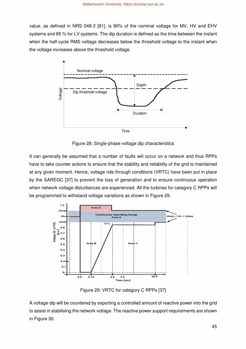
45
value, as defined in NRS 048-2 [81], is 90% of the nominal voltage for MV, HV and EHV
systems and 85 % for LV systems. The dip duration is defined as the time between the instant
when the half-cycle RMS voltage decreases below the threshold voltage to the instant when
the voltage increases above the threshold voltage.
Duration
Dip threshold voltage
Nominal voltage
Depth
Vol
tage
Time
Figure 28: Single-phase voltage dip characteristics
It can generally be assumed that a number of faults will occur on a network and thus RPPs
have to take counter actions to ensure that the stability and reliability of the grid is maintained
at any given moment. Hence, voltage ride through conditions (VRTC) have been put in place
by the SAREGC [37] to prevent the loss of generation and to ensure continuous operation
when network voltage disturbances are experienced. All the turbines for category C RPPs will
be programmed to withstand voltage variations as shown in Figure 29.
Figure 29: VRTC for category C RPPs [37]
A voltage dip will be countered by exporting a controlled amount of reactive power into the grid
to assist in stabilising the network voltage. The reactive power support requirements are shown
in Figure 30.
Stellenbosch University https://scholar.sun.ac.za

46
Figure 30: Reactive power support requirements for RPPs [37]
The windfarm has two control modes, voltage control and reactive power control mode. If the
plant exports more than 5% of maximum active power then the plant is automatically controlled
in voltage controlled mode with a voltage set point of 135 kV. If the plant export less than 5%
of maximum power then the plant is controlled in reactive power control mode, and the reactive
power is taken down to 0 MVar at a certain slope. In other words the power factor is 1 in
reactive control mode. The reason is that Eskom bills RPPs according to their apparent power
usage and not just their active power usage. RPPs can assist in network stability through
reactive power support but due to the billing procedure in South Africa most RPPs limit reactive
power support.
Inverters as used in RPPs can be highly sensitive to voltage dips. Voltage dips can result in
various PQ problems such as the loss of control within an inverter [86] and tripping of inverters.
The tripping of inverters depends on its protection control settings and the type of dip. Dips
produced by capacitors energizing, motor starting and transformer energizing fall within the
design voltage tolerance requirements of the RPP and should not lead to operational problems
or equipment failure [86] due to the counter measures taken as described. This is shown in
Section 5.4.1.2.
2.8. MITIGATION METHODS TO REDUCE POOR PQ IN TRACTION NETWORKS
There is a wide range of mitigation methods in literature that can be used to improve the PQ
problems associated with traction loads discussed in Section 2.7. In this section some of the
mitigation methods mentioned in literature will be discussed briefly due to the large amount of
research already done on this topic.
Stellenbosch University https://scholar.sun.ac.za

47
2.8.1. Phase-shift method
One way in which voltage unbalance can be reduced is by connecting adjacent traction
substations to different phase pairs. This method is investigated in [53] and is found to
effectively reduce voltage unbalance if the railway sections are equally loaded [59]. This is not
the case in systems with dynamic power demand, in short railway sections and in railway
sections that contain a railway station. The phase-shift method is also an ineffective voltage
unbalance mitigation method in long rural lines with very little traffic, since a single locomotive
will be in service for the majority of the time. Hence the railway sections will not be equally
loaded. In most traction networks the phase-shift method is not an adequate mitigation method
on its own since the loads on a traction network cannot be distributed evenly [87]. This method
is already implemented in South Africa but will only be effective in certain network conditions.
It is certainly not the case in the traction network being investigated as it contains short railway
sections, with high traffic and dynamic power demand. The network of concern also contains
a railway station near the POC of the RPP.
2.8.2. Self-balancing traction transformers
One form of voltage unbalance mitigation is the implementation of special self-balancing
traction transformers to mitigate the unbalance of single-phase loads. Such transformers
include the V/v, Scott and Le Blanc transformers. The V/v traction transformer is connected to
the three-phase 132 kV, 50 Hz network using two single-phase transformers as shown in
Figure 31. The V/v traction transformer draws three-phase current, aI , bI and cI which supplies
two single-phase currents Iα and Iβ to traction loads on the railway system. The single-phase
transformers have a turn ratio of 1
2
N
N.
Figure 31: Traction power supply system with V/v traction transformer
cI bI aI
1N 1N
2N 2N
IαIβ
Stellenbosch University https://scholar.sun.ac.za

48
The Scott traction transformer is connected to the three-phase 132 kV, 50 Hz network through
a single-phase centre-tapped main transformer and a single-phase teaser transformer as
shown in Figure 32. The main single-phase centre tapped transformer has a turn ratio of 1
2
N
N.
The teaser transformer is connected to the centre tapped point of the main transformer and
has a turns ratio of 1
2
32
N
N.
Figure 32: Traction power supply system with Scott traction transformer
These special traction transformers have been investigated in [63], [88]–[90]. A comparison
between these transformers have been made in [53], [63]. A detailed comparison between the
Scott and Le Blanc transformers have been made in [91]. From the above comparisons it can
be concluded that all of the above traction transformers will reduce the voltage unbalance
compared to the conventional delta-wye transformer. The Scott and Le Blanc type provide the
best voltage unbalance mitigation but are more expensive compared to the V/v type due to
their complex structure. Therefore, it was concluded that the V/v transformer provides the best
performance and cost option for traction substations.
The use of self-balancing traction transformers do not remove voltage unbalance completely
due to the dynamic power demand of traction loads that lead to railway sections that are
unequally loaded [14], [21]. Self-balancing traction transformer will be most effective in heavy
traffic railway lines that do not contain a railway station. Furthermore, the self-balancing
transformers are incapable of compensating for reactive power and harmonics. Methods to
compensate for voltage unbalance, harmonics and reactive power are hence required.
It should be noted that there is a trade-off between cost and performance when utilizing the
above mentioned self-balancing transformers. These transformers provide better performance
132 kV, 50 Hz
Overhead
catenary
Rails
A
B
C
aIbIcI
IαIβ
1N
2N
1
32
N
2N
Stellenbosch University https://scholar.sun.ac.za

49
compared to the conventional delta-wye transformers but are more expensive thus leading to
most substations utilizing conventional delta-wye transformers. It is important to mention that
conventional delta-wye transformers are currently being used in South Africa traction
substations. A recommendation that can be made is to implement self-balancing transformers
at points in the network where voltage unbalance is a big problem.
2.8.3. Passive filter and reactive power compensation
Passive compensation methods such as reactive power compensation capacitors and passive
filters can be used for reactive power and harmonic compensation. In [70] a passive filter
control scheme was proposed for co-simulation of single tuned filters to reduce low-order
harmonics and reactive power compensation and a high-order filter to reduce high-order
harmonics and harmonic resonance in the power system. Passive filters are limited to a
number of harmonic orders and are normally designed for specific applications. Moreover,
passive filters are designed for fixed reactive power compensation, therefore, a thyristor
controlled reactor combined with a passive filter is proposed in [92] to control the amount of
reactive power compensation. Passive filters, however, are not ideal for traction loads due to
their inability to compensate for dynamic load changes [93] and thus the need for more
advanced compensation methods are required. Passive filters are unable to compensate for
voltage unbalance which is the major concern of traction loads. Active filters provide the best
harmonic compensation but are more expensive.
2.8.4. Dynamic compensation methods
The inability to completely mitigate voltage unbalance by using the phase-shift method or by
installing a self-balancing traction transformer, has led designers to utilize dynamic
compensation devices such as static VAR compensators (SVCs) or static synchronous
compensators (STATCOMs). Dynamic compensation provides a more effective solution for
loads that have dynamic characteristics such as traction loads.
Different SVCs have been widely used for voltage unbalance and reactive power
compensation [94]–[97]. SVCs can rapidly compensate by supplying or absorbing reactive
power. This is done by controlling the firing angle of the fixed-capacitor/thyristor reactor based
on the voltage and current of the network. In an unbalanced system, a SVC may not provide
adequate compensation as it most likely requires asymmetrical control of the thyristor fire
angles. In addition, SVCs do not provide the required tracing capabilities to compensate for
dynamic voltage unbalance changes [98]. Other disadvantages of SVCs are harmonic current
injections caused by an unbalance system, and resonance between the shunt capacitor and
the network inductance [99], [100]. In an unbalanced system, the current magnitude of the
three SVC branches will be different which will cause large current harmonic distortion
Stellenbosch University https://scholar.sun.ac.za

50
(particularly, the third harmonic) in the system [100]. Various different SVC types have been
investigated in [101] with the purpose of obtaining the SVC type with the best performance
with regards to the harmonic and resonance impact to the network. STATCOMs provide better
voltage unbalance compensation compared to SVCs but are generally not widely used as they
require more complex control and are more costly. In addition, SVCs are unable to compensate
for harmonics. Figure 33 shows a traction power supply system with a SVC.
Figure 33: Traction power supply system with conventional SVC
A more improved compensation method for railway applications utilising back-to-back single-
phase PWM converters and a coupled DC link capacitor have been proposed in [102]. It is
132 kV, 50 Hz
Overhead
catenary
Rails
A
B
C
aIbIcI
IαIβ
Traction transformer
Stellenbosch University https://scholar.sun.ac.za

51
more commonly known as a railway power static conditioner (RPC) and the connection of a
RPC in a traction power supply system is shown in Figure 34.
Figure 34: Traction power supply system with RPC
The RPC is connected to two phases of a traction transformer’s secondary winding. RPCs can
compensate for voltage unbalance, harmonic current and reactive power of traction loads by
injecting a controlled current into the traction feeder. The DC link capacitor allows the flow of
active and reactive power between the converters and thus in both phases of the traction
network. RPCs provide significant voltage unbalance compensation [53]. RPCs can has the
ability to completely compensate for voltage unbalance. Another advantage of the RPC is its
ability to operate regardless of the traction transformers connection type. The high capacity
needed for complete compensation of dynamic traction loads and the high cost of the RPCs
compared to other compensation methods will limit the utilization of this method in traction
applications. A number of modified compensators based on the RPC have been proposed for
further research and development to decrease the overall cost of the system while maintaining
the same level of performance of a RPC. A simplified half-bridge RPC has been proposed in
[98], which utilizes two half bridge converters coupled by two DC link capacitors. Another
modified RPC type of compensator that consist of a three wire, 6 switch converter and a Scott
traction transformer, more commonly known as active power quality compensator (APQC) has
been proposed in [93]. The proposed APQC connects to the traction system that is supplied
aIbIcI
IαIβ
Stellenbosch University https://scholar.sun.ac.za

52
by the Scott transformer. This method of compensation transforms two single-phase
orthogonal voltages to three-phase symmetrical voltages. Due to the wide use of V/v
transformers in railway applications a similar method that can transform two single-phase non-
orthogonal voltages to three-phase symmetrical voltages was required. An improved APQC
compensator that operates with a V/v transformer has been proposed in [89].
Co-phase systems are proposed in [103], [104] which utilises a self-balancing transformer in
combination with a RPC and can be seen as a modified APQC. A co-phase system reduces
the amount of neutral sections in the railway network by half which has various advantages.
The remaining neutral sections can be replaced by insulators for safety purposes. The
insulation requirements and length of insulators can thus be reduced [104]. Consequently,
locomotives do not need to be switched off that often and can be switched off for a smaller
duration. Also locomotives do not need to change operation conditions that often and PQ
impact will decrease. However, to achieve complete compensation a power converter with a
large rating is required leading to a high cost system. Various hybrid co-phase systems have
been proposed to achieve the same level of compensation through a power converter with a
smaller rating [105]–[107]. Consequently, leading to a system with a decreased overall cost.
An advanced co-phase system are proposed in [108] which is another configuration type of
the conventional co-phase system. In the advanced co-phase method the traction system is
supplied through a three-phase and single-phase converter rather than a self-balancing
transformer. This method of compensation provides the capability of removing all neutral
sections in the railway network. The traction loads therefore becomes less dynamic and the
need for frequent changes in the operating conditions of locomotives are reduced. The
complete railway system is powered through the converters which will lead to high cost and
low reliability.
SVCs is a low cost dynamic compensator compared to STATCOMs, active power filters and
APQCs.
2.9. CONCLUSION
This chapter presented the reader with background on the working principles of traction loads
in South Africa. The dynamic behaviour of traction loads are mathematically described to gain
insight into the characteristics of traction loads. The PQ issues associated with traction loads
and the possible PQ impact these issues can have on RPPs are investigated. To investigate
the impact that poor PQ in traction networks will have on the PQ assessment of RPPs the
standards used for PQ management and assessment in South Africa are presented. Finally, a
brief overview is given on possible mitigation methods that can be used to reduce poor PQ in
traction networks.
Stellenbosch University https://scholar.sun.ac.za

53
CHAPTER 3
SIMULATION MODELS
3.1. INTRODUCTION
Modern AC railway networks are complex in nature as they contain various characteristics,
such as dynamic moving loads, single-phase supply and railway earthing, which can have a
big impact on the national power supply in terms of PQ. These railway networks are connected
to a larger electrical power supply system, in this case Eskom national grid that contains RPPs
which further add to the complexity. It is important that the combination of these systems be
designed and analysed as accurate as possible to minimise the possibility of future problems.
This has come apparent with the introduction of renewables to the national grid and their
increased rate of connection. The design, maintenance, management and planning of a power
system is a difficult task that requires high accuracy and efficiency. Software tools enable the
electrical engineer to analyse and simulate these systems for the optimal solution. In addition,
software tools offer the advantage of investigating the network and finding various solutions
prior to any physical change to the network infrastructure and is thus essential in network
planning.
Various software tools are available for modelling of power systems such as DIgSILENT
PowerFactory, Matlab/Simulink and PSCAD. It was deemed necessary that the software tool
of choice provide high functionality, capable of simulating large power systems in the time
domain. Eskom utilise both PSCAD and DIgSILENT PowerFactory as simulations tools. Most
of the original equipment manufacturer time domain models of RPPs have been done in
PSCAD as it provides the best functionality for time domain modelling. PSCAD, however, lacks
the capability in modelling large power systems. Therefore, the need exist in utilising
DIgSILENT PowerFactory for time domain modelling of RPPs as it provides high functionality
in large power system modelling. Eskom mostly use DIgSILENT PowerFactory for power
system stability simulations and network planning which further highlights the need for
accurate RPP and traction load models for future network studies in DIgSILENT PowerFactory.
Eskom is continually working on updating and improving there DIgSILENT PowerFactory
distribution models. Therefore, DIgSILENT PowerFactory will be used as the PQ analysis
software for this thesis.
It is important to understand the functions, limitations and assumptions inherent in software
implementation. Therefore, an overview of the functions and limitations of DIgSILENT
PowerFactory will be presented. Methods will be investigated to overcome these limitations.
Stellenbosch University https://scholar.sun.ac.za

54
It is known that the accuracy and quality of output of any simulation is directly proportional to
the accuracy and quality of the input variables. Typical input variables required for accurate
RPP (inverter) and traction (rectifier) system modelling include:
• Power system information such as system configuration and three-phase fault levels.
• Cables, overhead lines and catenary system information and impedance ratings.
• Transformer information such as rating, phase connection impedance and tap settings.
• Train traffic timetable with start, stop, dwell and passing times.
• Locomotive drive ratings such as motor rating, weight, acceleration and maximum
speed.
• Turbine passive filter information such as configuration and rating.
• Locomotive passive filter information such as configuration and rating.
At the time of writing limited information was available with regards to locomotive drives and
filter equipment ratings. Therefore, various assumptions and simplifications had to be made.
To understand the PQ impact of traction loads on the network and on RPPs it is necessary to
model locomotive rectifiers in detail, so to investigate various effects that a rectifier can have
on the network. In this chapter the theory, control, modelling and implementation of the two
main locomotives technologies types identified in Section 2.2 will be presented. Therefore, an
active rectifier and half-controlled thyristor rectifier will be designed and implemented in
DIgSILENT PowerFactory. It is important that the simulation models reflect the physical system
as closely as possible. These traction load models will provide insight on the working principles
of traction loads and describe the PQ issues related to traction loads.
RPP manufacturers protect their designs by not disclosing all parameter values and other
design detail. Therefore, to completely understand the PQ impact on RPPs it is necessary to
model inverters in detail, so to investigate various effects that an inverter can have on the
network and vice versa, rather than using the available customer models. In this chapter the
modelling of a generic conventional PWM inverter, interleaved PWM inverter and a hysteresis
controlled inverter along with their respective implementation in DIgSILENT PowerFactory will
be discussed.
The purpose of all these models are to perform time domain simulations to model the dynamic
PQ behaviour of traction loads in detail and with a high degree of accuracy. In time domain
simulations the voltages and currents are expressed as instantaneous values. Therefore, the
individual harmonic content of voltage and current waveforms can be accurately expressed
and compared to PQ measurements conducted on the network. The assumptions and
simplifications that were required in the design and implementation of generic RPP (inverter)
and traction (rectifier) models in DIgSILENT PowerFactory will be discussed.
Stellenbosch University https://scholar.sun.ac.za

55
3.2. OVERVIEW ON DIGSILENT POWERFACTORY
DIgSILENT GmbH, is a German software and consulting company that provides a wide variety
of electrical engineering services in the field of power systems. They develop DIgSILENT
PowerFactory, a Windows-based integrated analysis software package for power system
simulation in industrial plants, generation, transmission, distribution and smart grids. Eskom
Distribution has obtained a corporate licence for DIgSILENT PowerFactory in 2003 after a
comprehensive evaluation of all the technical operations offered [109]. DIgSILENT
PowerFactory caters for the full range of standard power system analysis needs to vastly
refined applications in modern technologies such as wind power, performance monitoring for
system testing and real-time system simulation [110], [111]. PowerFactory is easy to use with
advanced solution algorithms combined with comprehensive and flexible modelling capabilities
that include a large suite of libraries and electrical power equipment models. Users are able to
design and create dynamic models for time domain simulations. Therefore, providing the user
with the required tools to undertake a grid impact analysis on wind farms and solar PV plants
to determine their PQ impact on the grid and vice versa. Consequently, DIgSILENT
PowerFactory has become the industry standard in utility and RPP simulations in South Africa
as most RPPs are connected to the Eskom distribution network.
DIgSILENT PowerFactory is capable of performing balanced and unbalanced power flow
studies, protection coordination of relays, short circuit analysis, long-term quasi dynamic load
flow simulations, etc. Some of the functions more relevant to PQ studies include [111]:
• Harmonic analysis which includes harmonic load flow, frequency sweep, flicker
calculation and harmonic distortion analysis.
• Balanced and unbalanced stability analysis in RMS or EMT dynamic simulations.
• Dynamic simulation language (DSL) modelling of dynamic models.
• The ability to model any combination of single-phase AC, three-phase AC and DC
network topologies, which will be important to model single-phase traction loads.
DIgSILENT PowerFactory also support scripting features that include the complete integration
of the built-in C++ style DIgSILENT programming language and open source Python
programming languages. Scripting is generally used to access objects and to automate tasks
which require the execution of time-consuming simulations e.g. short circuit sweep [112], [113].
However, the application can be used for far more than that such as inserting external
parameter characteristics from a comma-separated values format file, processing results,
exporting results and plots to excel, changing parameter values within the code, etc.
Stellenbosch University https://scholar.sun.ac.za

56
3.2.1. DIgSILENT PowerFactory limitations
DIgSILENT PowerFactory is not designed for simulating and analysing railway networks but
rather for analysing general power systems. The traction network of a railway system is
simulated and analysed as an electrical power system rather than a detailed locomotive rolling
stock model. Therefore, DIgSILENT PowerFactory lacks the capability to model and simulate
moving AC traction loads along a railway network. Consequently, challenges exist in simulating
dynamic models of traction loads in the time domain. Moving DC traction loads in DIgSILENT
PowerFactory has been simulated in [114] and a similar approach could be implemented for
AC traction systems. The modelling and implementation of moving dynamic models, however,
is out of the scope of this thesis.
DIgSILENT PowerFactory does not contain a built-in model for a half-controlled thyristor
rectifier and thus a method had to be explored to obtain the required functionality of a half-
controlled thyristor rectifier. This challenge is further increased by a lack in DIgSILENT
PowerFactory to simulate the combination of an AC and DC system. A method to overcome
these limitations is presented in Section 3.5.2.
3.2.2. RMS and EMT simulations
It was already stated that the models need to be analysed in time domain and that DIgSILENT
PowerFactory provide the user with two dynamic simulation functions: RMS, which are used
for three-phase networks under steady state conditions for mid- to long-term transient analysis
and EMT, which are used for three-phase dynamic networks for short-term electromechanical
and electromagnetic transient analysis [115].
In RMS simulations the voltages and currents are expressed as phasors in frequency-domain.
Therefore, the voltage and current equations are represented as follows [116]:
and V jwLI I jwCV= = (2.32)
In EMT simulations the voltages and currents are expressed by their instantaneous values in
time-domain. Therefore, the voltage and current equations are represented by differential
equations as follows [116]:
and di dv
v L i Cdt dt
= = (2.33)
EMT simulation present a closer representation of the physical world due to the simulation
domain. Furthermore, in EMT simulations the network dynamics and events can be simulated
with a greater degree of accuracy in both short-term transient analysis as well as with longer-
term transient analysis. Trains move past substations and renewable plants at a high speed,
therefore, making the measured data at the site inaccurate due to aggregated 10-minute
Stellenbosch University https://scholar.sun.ac.za

57
values based on frequency-domain rms values. Therefore, it is important to analyse the short-
term effect of traction loads on RPPs as the impact of traction loads will be instantaneous thus
making EMT simulations preferable. However, it must be stated that due to the increase in
dynamic simulation of all passive network elements that the simulation time will be increased
significantly [115].
3.3. DIGSILENT POWERFACTORY BUILT-IN MODELS
It was already stated that DIgSILENT PowerFactory provides a global library with a wide range
of components that includes predefined built-in equipment models. In addition, DIgSILENT
PowerFactory provide the user with the possibility to design and construct mathematical and
graphical composite models through DSL by using the available predefined equipment models
as well as user defined common models. These user defined composite and common models
can be connected to network elements. In this section the relevant predefined built-in
equipment models that were implemented in the models and do not need to be designed using
DSL will be discussed in more detail.
3.3.1. PWM converter model
The built-in PWM converter model (ElmVsc) is used to model rectifiers and inverters within
DIgSILENT PowerFactory. In EMT simulation the built-in PWM converter can be modelled and
controlled in two different ways: as a controlled voltage source or a detailed model. For the
controlled voltage source model the PWM converter is represented by a self-commutated
three-phase voltage source converter (VSC) as shown in Figure 35. Note, however, that for
the controlled voltage source model the three-phase VSC in Figure 35 does not contain actual
switches. A DC link capacitor is not included within the PWM converter model and has to be
added externally.
Figure 35: PWM converter model with series reactance, no-load losses and load losses
For the detailed model the three-phase VSC in Figure 35 is represented by a three-phase
detailed VSC composed out of IGBT switches and is similar to the three-phase VSI equivalent
diagram as seen in Figure 19. Note that the external DC link capacitor and DC voltage source
in Figure 19 is not included in the detailed PWM converter model and must be added externally.
DCV R
RL
ACV
+
−
Stellenbosch University https://scholar.sun.ac.za

58
3.3.1.1. Modelling of PWM inverter losses
A grid-connected PWM inverter is connected to the grid through a reactance, therefore, the
AC series reactance is included within the built-in PWM converter model to simplify modelling.
Both no-load and load losses models are included in the PWM converter model. No-load or
switching losses are represented and modelled by a shunt resistance between the DC
terminals. Furthermore, load losses are represented and modelled as a series resistance on
the AC side. Refer to Figure 35 for the equivalent circuit of the built-in DIgSILENT Powerfactory
PWM converter model with series reactance and losses represented.
3.3.1.2. Load flow control conditions of PWM converter
The load flow analyses results of the PWM converter depend on the chosen control condition.
DIgSILENT PowerFactory provide various control conditions that are supported by the PWM
converter. The description and general application of each condition are defined below [47]:
• ACV - phi : The AC terminal magnitude and phase are specified. This is generally used
with motor-side converters in variable speed drives.
• DCV - phi : The magnitude of DC voltage and phase of AC terminals are specified.
There is no typical application for this condition.
• PWM - phi : This condition provide no control as the magnitude and phase of the
amplitude modulation factor are directly set.
• DCV - Q : The magnitude of the DC voltage and reactive power output are set. This
control condition result in various common application such as STATCOM and a VSC
for high voltage direct current (HVDC) applications.
• P - ACV : The magnitude of the AC voltage terminals and active power output are set.
This control condition result in common applications such as grid-side converter of
converter driven synchronous machines and VSC-HVDC.
• P - Q : The active power and reactive power output is set at the AC output. Similar
typical applications as described in the P - ACV control condition.
• DCV - ACV : The magnitude of DC voltage and AC voltage. Similar typical applications
as described in the DCV - Q control condition.
• P - cos( )phi : The active power at AC output and power factor are specified. Typical
application with PWM grid-connected converters for renewables.
• DCV - cos( )phi : The magnitude of DV voltage and power factor are specified. Typical
applications include VSC-HVDC and renewable implementations.
Stellenbosch University https://scholar.sun.ac.za

59
3.3.1.3. RMS and EMT control of PWM converter – controlled voltage source
model
For the controlled voltage source model, at fundamental frequency, the ideal PWM converter
is modelled as a DC controlled AC voltage source and the following voltage equations are
applicable to the PWM converter when operating within the linear region ( mP ≤ 1) [118]:
, 0
, 0
AC r mr DC
AC i mi DC
V K P V
V K P V
=
=
i i
i i (2.34)
where, ,AC rV and ,AC iV represent the real and imaginary RMS values of the AC voltage, DCV
the DC voltage, mrP and miP the real and imaginary values of the amplitude modulation index
and 0K a constant gain depending on the ratio between the DC and AC voltage as well as the
type of modulation used. The PWM converter model supports both sinusoidal modulation for
a sinusoidal PWM inverter as well as rectangular modulation for a square wave inverter [118].
For a sinusoidal PWM inverter, 0K is:
0
3
2 2K = (2.35)
For the controlled voltage source model, the PWM amplitude modulation index mP (magnitude
and phase), in RMS and EMT simulations, can be controlled through different input signals,
depending on the type of application [118]:
• mrP and
miP : In this method, the real and imaginary values of the PWM amplitude
modulation index are used as inputs. The reference frame for this method is the global
reference frame. Therefore, the PWM controller inputs must be used in combination
with reference frame transformations in addition to phase measurement devices such
as phase-locked loop (PLL) to measure cosref and sinref for accurate
transformations.
• mdP , mqP , cosref and sinref : mP is defined in a reference frame specified by cosref
and sinref . This method can typically be used for grid-connected applications where
the system is implemented in the dq reference frame in combination with a PLL.
• ,d refi , ,q refi , cosref and sinref : The reference d- and q-axis current values can be used
as inputs to the PWM converter when the internal current controller of the PWM
converter model is used. The current input variables are defined in a reference frame
specified by cosref and sinref .
• ,m inP and phiud : The magnitude and phase of mP are used as inputs. This method is
essentially equivalent to the mrP and
miP method.
Stellenbosch University https://scholar.sun.ac.za

60
• ,m inP and 0f : Here the magnitude of mP and frequency of output signals can be
specified.
The controlled voltage source model contain an optional internal current controller. The internal
current controller is the simplest implementation of a current controller. The input currents di
and qi are simply the output AC currents of the PWM controller defined in a reference frame
specified by cosref and sinref . Therefore, the output signals mdP and mqP , which are also
defined in the same reference frame, are transformed back to the global reference frame within
the controller by using cosref and sinref . The additional input current signals, ,d refi and ,q refi ,
are found through an active and reactive controller. Refer to Figure 36 for the block diagram
of the internal current controller.
Figure 36: Block diagram of the built-in current controller in the PWM controller model
The controlled voltage source model can also be controlled through an external current
controller and will be discussed in more detail where relevant. Losses can be added to the
controlled voltage source model according to Section 3.3.1.1.
3.3.1.4. RMS and EMT control of PWM converter – detailed model
For the detailed model, the PWM converter is represented by a three-phase detailed VSC
composed out of IGBT switches and is, therefore, similar to the three-phase VSI equivalent
diagram as seen in Figure 19. The switching states au , bu and cu of the detailed PWM model
can be externally controlled through a DSL model. These signals control the on/off states of
the three-phase legs. A positive signal for au , bu and cu will connect the respective phase to
the positive DC voltage DCV and vice versa. It is important to note that the internal current
,d refi
,q refi
di
qi
mdP
mqP
Stellenbosch University https://scholar.sun.ac.za

61
controller is not available for this approach, therefore, an external current controller must be
designed and implemented with DSL.
3.3.1.5. PWM converter model limitations
The DIgSILENT PowerFactory PWM controller is a three-phase model, therefore, challenges
exist in single-phase applications such as the control of single-phase active rectifiers. A
method had to be investigated to overcome this limitation by controlling each phase separately.
The implementation of the solution will be discussed in more detail in Section 3.5.1.
3.3.2. AC and DC cables
The AC overhead lines can all be defined as either short-length or medium-length lines as all
of the relevant lines in the network are no longer than 240 km. Short-length and medium-length
lines can be modelled using lumped parameters with a small effect on the accuracy of
simulation as shown in [119]. The AC cable parameters are obtained from the Wind farm A
original equipment manufacturer model of the renewable plant.
3.3.3. Built-in PLL model
DIgSILENT PowerFactory contain a built-in PLL DSL model that is supported for both RMS
and EMT simulations within DIgSILENT PowerFactory. The PLL element (ElmPhi__pll) is used
to measure the frequency and phase of the system voltage and then to output cosphi and
sinphi as output signals to the rest of the control system.
3.3.4. Built-in sample and hold element
DIgSILENT PowerFactory contain a built-in sample and hold element (ElmSamp) that is
supported for both RMS and EMT simulations within DIgSILENT PowerFactory. The sample
and hold element is used to sample an analog signal for digital control purposes. The input
analog signal is sampled at every rising edge of the clock pulse input signal and is held
constant up to the next rising edge. Therefore, ElmSamp can be setup for symmetrical or
asymmetrical regular sampling as described in Section 2.4.4.2 by controlling the clock pulse
input signal.
3.3.5. Built-in voltage measurement element
DIgSILENT PowerFactory contain a built-in voltage measurement element (StaVmea) that is
supported for both RMS and EMT simulations within DIgSILENT PowerFactory. The voltage
measurement element can be used to measure AC or DC voltage at any selected terminal.
The number of phases (three-phase or single-phase) for an AC measurement can be selected
along with the voltage rating and frequency output. The measured voltage can then be fed as
Stellenbosch University https://scholar.sun.ac.za

62
a signal to the rest of the control system. The measured voltage are transformed into a fixed
two-axis reference frame (αβ reference frame). Therefore, the following StaVmea output
signals can be used in a control system during EMT simulations: real voltage (ur ), imaginary
voltage (ui ), voltage magnitude (u ), zero sequence voltage ( 0u ) and the frequency ( fe ).
3.3.6. Built-in current measurement element
DIgSILENT PowerFactory contain a built-in current measurement element (StaImea) that is
supported for both RMS and EMT simulations within DIgSILENT PowerFactory. The current
measurement element can be used to measure AC or DC current at any selected cubicle of
an element connected to a terminal. The number of phases (three-phase or single-phase) and
current rating can be selected for an AC measurement. The measured current can then be fed
as a signal to the rest of the control system. The measured voltage are transformed into a fixed
two-axis reference frame (αβ reference frame). Therefore, the following StaImea output signals
can be used in a control system during EMT simulations: real current ( ir ), imaginary current (
ii ), current magnitude ( i ) and zero sequence current ( 0u ).
3.3.7. Built-in power measurement element
DIgSILENT PowerFactory contain a built-in power measurement element (StaPqmea) that is
supported for both RMS and EMT simulations within DIgSILENT PowerFactory. The power
measurement element can be used to measure the power flow of any element connected to a
terminal. The number of phases (three-phase or single-phase), power rating and orientation
can be selected. For EMT simulations the power measurement element will measure the
phase voltages and currents and output the real power ( p ) and reactive power ( q ) as output
signals to the control system.
3.4. CONTROL OF CONVERTER - POWER FLOW THEORY
An active rectifier is basically an inverter connected to a network through a series inductor.
The control of an active rectifier or inverter has been described in various papers [120], [121].
A grid-connected inverter with a series reactance can be illustrated by two voltage sources
and a pure inductance as seen in Figure 37 to derive the required power flow equations. The
direction of the current I determine whether the converter is operating as an inverter or as a
rectifier.
Stellenbosch University https://scholar.sun.ac.za

63
Figure 37: Power flow between two voltage sources
The inverter mode of operation is described below. The current flowing from an inverter I
acting as voltage source iV to the grid represented by sV through the filter inductive reactance
X can be calculated as follows:
( )
090
90 90
i s i s
si
V V VI
XX
X
V
VV
X
δ
δ
− ∠ − ∠ °=
∠ °
∠ − ° − ∠ −
=
= °
(2.36)
The apparent power flowing from the inverter side iS can be calculated as follows:
( )
( )2
90 90
90 90
sii i i
i si
VV
VV
S V I VX X
V
X X
δ δ
δ
∗ = = ∠ ∠ ° − ∠ °
= ∠ ° − ∠ ° +
−
(2.37)
Per definition the real power at the inverter iP can be calculated as follows:
( )
( )
2
cos 90 cos 90
sin
cos i sii i
i s
VV VP S
X X
V
X
V
φ δ
δ
= = ° − ° +
=
(2.38)
The reactive power at the inverter iQ can be calculated as follows:
( )
( )
2
2
sin 90 9sin s 0
c
in
os
i sii i
i si
VQ S
X X
V
X X
VV
VV
φ δ
δ
= = ° − ° +
= −
(2.39)
The apparent power flowing into the network sS can be calculated as follows:
iV δ∠ 0sV ∠ °
90X∠ °
0I∠ °
Stellenbosch University https://scholar.sun.ac.za

64
( ) ( )
( ) ( )2
0 90 90
90 90
sis s s
s i s
S V I VX X
V
X X
VV
V V
δ
δ
∗ = − = ∠ ° ∠ ° + ∠ °
= − ∠ ° − + ∠
− −
°
(2.40)
Per definition the real power flowing into the source sP can be calculated as follows:
( ) ( )
( )
2
coscos cos 90 90
sin 0 sin
s i ss s
i s i s
VP S
X X
V
V V
X
V VV
X
φ δ
δ δ
= = − ° − +
= − −
°
+ =
(2.41)
The reactive flowing into the source sQ can be calculated as follows:
( ) ( )
( )2
2
sin sinsin 90 90
cos
s i ss s
s i s
V VVQ S
X X
V
X
V V
X
φ δ
δ
= = −
= −
° − + °
(2.42)
To inject power at unity power factor into the source the current should have the same angle
as the voltage at the source. To illustrate this graphically, Figure 38 shows a scaled phasor
diagram of a single-phase system in inverter mode of operation.
Figure 38: Voltage and current phasor diagram for inverter mode of operation
Figure 39 shows a scaled phasor diagram of a single-phase system in rectifier mode of
operation.
δ
0I∠ °
iV δ∠
0sV ∠ °
90IX∠ °
Stellenbosch University https://scholar.sun.ac.za

65
Figure 39: Voltage and current phasor diagram for rectifier mode of operation
The inverter voltage exceeds the grid voltage to produce the reactive power consumed by the
reactance when transferring the required active power. The power factor can be controlled at
unity by ensuring that all reactive power is consumed in the reactance and that the reactive
power consumed at the grid is zero. The inverter voltage vector iV magnitude and phase angle
values for unity power factor at the grid interface are subsequently calculated.
By setting 0I I= ∠ ° in (2.36):
( )90 90 0
cos0
cos
si
i s
si
I IX
V
V
V
V
V
X
V
X
δ
δ
δ
= ∠ − ° − ∠ − ° = ∠ °
=
⇒ =
−⇒ (2.43)
The value of δ for a required sP can be calculated from (2.41):
2 2
2
tan
ar
sin
sinc
c a
s
t
o
n
i ss
s s
s
s
VP
X
V
P
V V
X X
X
V
δ
δδ
δ
δ
= =
⇒ =
=
(2.44)
Now the value of iV can be calculated from (2.43):
2arctcos an
si
s
s
VV
X
V
P=
(2.45)
The above power theory equations can also be used to model an active rectifier by changing
direction of current flow and in turn changing δ to a negative value as illustrated in Figure 39
for rectifier mode of operation.
δ180I∠ °
iV δ∠ −
0sV ∠ °
90IX∠ − °
Stellenbosch University https://scholar.sun.ac.za

66
3.5. TRACTION LOAD (RECTIFIER) MODELLING
The aim of the modelling is to control the rectifier so that the rectifier is supplying power to the
traction motors but in turn injecting harmonic currents into the grid. This will provide a method
to study the effects of traction on the PQ under various supply conditions.
3.5.1. DIgSILENT PowerFactory active rectifier model
3.5.1.1. Overview
Locomotives on the 25 kV AC traction systems use single-phase active rectifiers to convert
power to DC. Three-phase inverters in the form of variable speed drives use the DC to control
AC motors on the axes of the locomotives. On the AC side the 25 kV voltage is converted to
1.5 kV by means of a single-phase transformer located in the locomotive. The DC bus between
the rectifier and the drive has a nominal voltage of 3 kV. The rectifier has a nominal power
rating of 12 MW (based on the actual maximum demand of the locomotives that are in service
on the network), therefore, sP is selected as -12 MW, i.e. nominal current I of -8 kA. A 50 Hz
filter reactance of 15% short circuit impedance was arbitrary selected, i.e. an inductance of
0.09 mH. By using these values in (2.38), (2.39) and (2.42) the relationship between power
and phase angle is plotted in Figure 40.
Figure 40: Active and reactive power magnitude as a function of δ
Figure 40 is further exposed around the operating point of this inverter and is shown in Figure
41. This is around the operating point (highlighted section) of 0.1489 radδ = − , from (2.44),
where the inverter power 12 MWsP = − . The negative power indicates that it is operating as
an active rectifier. The inverter voltage is set to 1.5168 kV, calculated from (2.45) to generate
the required reactive power ( 1.8 MVARiQ = ) so that the reactive power at the source side can
Stellenbosch University https://scholar.sun.ac.za

67
be zero. Although power flows from the grid to the inverter, reactive power is still generated by
the inverter as long as the inverter can generate a voltage magnitude that exceeds the grid
voltage, i.e. it has a high enough DC voltage.
Figure 41: Active and reactive power magnitude as a function of δ around operating point of
0.1489 radδ = −
Figure 42 shows the designed control layout of a single-phase active rectifier.
Figure 42: Designed control layout of a single-phase active rectifier
Three-phase VSI
PLL
-+
PI+
PI
PWM Comparator
-Block
generator
Sawtooth
generator
++
K
L
iV δ∠ 0sV ∠
,s aV
aI
DCV DCC
DCV
au cubu
aS
cosphi
refV
saw
cl
_i r
Stellenbosch University https://scholar.sun.ac.za

68
Basic functionality can be shown in the time domain using the DIgSILENT PowerFactory EMT
tool.
3.5.1.2. Element layout in DIgSILENT PowerFactory
Figure 43 shows the network diagram of the system. Both the AC and DC sides are modelled
by simple voltage sources. The network further consist of a single-phase 132/25 kV traction
transformer, single-phase 25/1.5 kV locomotive transformer, an AC LC filter and DC capacitor.
Refer to Figure 174 in the appendix for a photo of the traction transformer nameplate. The
power that flows between these sources is a function of the selected phase angle.
Figure 43: Network diagram of the single-phase active rectifier traction system
3.5.1.3. Composite model in DIgSILENT PowerFactory
Figure 44 shows the designed composite model of the active rectifier system consisting of a
voltage measurement slot, a current controller, voltage controller, sample and hold element
and the inverter.
Stellenbosch University https://scholar.sun.ac.za

69
Figure 44: Designed composite model of the single-phase active rectifier in PowerFactory
The built-in PWM converter model (ElmVsc) discussed in Section 3.3.1 is used as the inverter
model in the implementation. The detailed model of the PWM converter, as discussed in
Section 3.3.1.4, is implemented due to the fact that the PWM converter lack the capability for
single-phase control. Therefore, the internal current controller of the PWM model is not
available for implementation in the single-phase active rectifier application and an external
current controller had to be designed and implemented. The current controller and voltage
controller is designed using DSL common models. The initialisation of these DSL models can
be challenging due to stability issues. Therefore, the initial conditions need to be set up with
great care to accurately evaluate the performance of the designed system during transient and
steady state conditions.
The current controller generates pulse width modulated signals to drive the inverter. For
optimal dynamic response, an inverter normally has an inner current control loop that follows
a reference in phase with the grid voltage waveform. The current controller will be discussed
in more detail in Section 3.5.1.5. A voltage vector on the rectifier AC terminals is synthesized
by generating pulse width modulated signals at a switching frequency sf . Note that the
switching frequency is unknown and will thus be chosen by examining the frequency spectrum
of the measured phase current in a traction substation which is shown Section 6.6.2. The
voltage measurement element in Figure 44 measures the grid voltage, with the predefined
built-in PLL model (ElmPhi__pll) discussed in Section 3.3.3, as a per unit value which is fed as
a signal to the current controller. The measured AC current in kA is sampled twice per switching
cycle, i.e. using asymmetrically regular sampling, and is then fed to the input of the current
Stellenbosch University https://scholar.sun.ac.za

70
controller. Asymmetrical regular sampling is done using the predefined built-in sample and
hold element (ElmSamp) discussed in Section 3.3.4. The reference block can be used to import
an external data file to change the nominal DC voltage in time domain to investigate the impact
of the DC voltage on the control and harmonics.
3.5.1.4. DSL model of voltage controller in DIgSILENT PowerFactory
The designed voltage controller in Figure 45 receives the measured DC voltage signal as a
per unit value and compare it to a reference voltage of 1 per unit. The per unit error is then
scaled to a voltage value by multiplying the error with the nominal DC voltage of 3 kV. A
reference current signal is then obtained by multiplying the error with a proportional integral
(PI) controller.
Figure 45: Designed active rectifier voltage controller DSL model in DIgSILENT
PowerFactory
3.5.1.5. DSL model of current controller in DIgSILENT PowerFactory
The complexity of the current controller was prevented by only considering steady state
operation. The current controller have the following input signals: the measured DC voltage in
per unit, the measured AC grid voltage in per unit, a reference current and the measured
sampled AC current in kA. The designed current controller shown in Figure 46 scales the
measured grid voltage signal (v_m) in per unit to a signal with a voltage value (v_ac) by
multiplying it with 2121 which is the peak value of the 1.5 kV AC grid voltage. The next step is
to scale it to a value opposite to the gain of the inverter or 21213000
. The sampled measured AC
current signal (i_ms) is multiplied by 1000 to scale the kA signal to an A signal (i_m). The
current controller multiplies the measured per unit grid voltage (v_m) with the reference current
(i_r) and compares this to i_m. A block wave generator generate a clock pulse signal (dir) that
changes from 1 to -1 and vice versa every half of a switching period. The signal dir is, therefore,
used as the input clock pulse signal for the sampling of the measured AC current within the
sample and hold block in Figure 44. The saw tooth generator with a period T with a value of
Stellenbosch University https://scholar.sun.ac.za

71
1(4 )sf×
generates a triangular waveform (saw) with a frequency ( sf ). By comparing the
reference signal s to the triangle waveform signal saw, the pulse width modulated signals are
generated for phases A and B, i.e. au and bu . A positive signal switches on the top switch in
a phase leg, while a zero signal switches on the bottom switch. Only two phases of the three-
phase PWM inverter model is used and cu is consequently kept at 0 V.
Figure 46: Designed active rectifier current controller DSL model in DIgSILENT
PowerFactory
3.5.1.6. Working principle of an active rectifier in DIgSILENT PowerFactory
To illustrate the working principle of the active rectifier the switching frequency sf is chosen as
5 kHz and thus the period T of the sawtooth generator is equal to 0.00005. Figure 47 shows
the reference signal (s) which is compared to the generated triangular signal (saw) to generate
the phase A leg switching state ( au ) in Figure 48.
Stellenbosch University https://scholar.sun.ac.za

72
Figure 47: PWM generator reference and triangle signal
Figure 48: PWM generator reference and phase A switching signal
When the inverter is controlled as described above the current in Figure 49 is produced flowing
between the grid and the inverter voltage sources. This is due to the inverter voltage that lags
the grid voltage slightly that causes current to flow towards the inverter which is 180° out of
phase with the voltage. Note that positive current was defined as current flowing out of the
inverter. The measured inverter phase current waveform and grid voltage waveform is plotted
in Figure 49 and Figure 50 respectively.
Stellenbosch University https://scholar.sun.ac.za

73
Figure 49: Inverter current waveform
Figure 50: Grid voltage waveform
The voltage and current waveforms in Figure 49 and Figure 50 are multiplied to obtain the
instantaneous power values as shown in Figure 51. The power has an average value of
12 MW− that corresponds to designed value. It is shown that there is no reactive power
present since the instantaneous power waveform never crosses zero on the vertical axis.
Stellenbosch University https://scholar.sun.ac.za
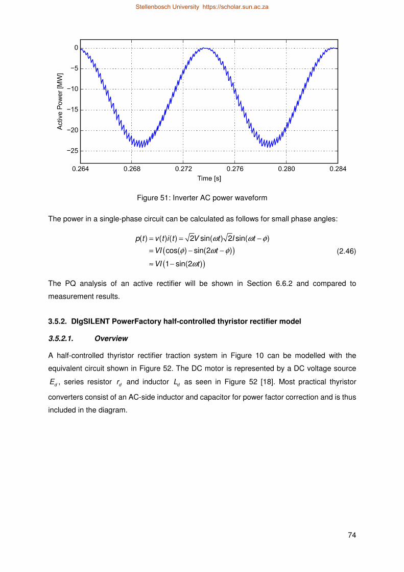
74
Figure 51: Inverter AC power waveform
The power in a single-phase circuit can be calculated as follows for small phase angles:
( )
( )
2 ) 2 sin( )( ) ( ) ( ) sin(
cos( ) sin(2 )
si ( )1 n 2
t tp t v t i t V I
VI
VI
t
t
ω ω φ
φ ω φ
ω
−
= −
≈ −
−
= =
(2.46)
The PQ analysis of an active rectifier will be shown in Section 6.6.2 and compared to
measurement results.
3.5.2. DIgSILENT PowerFactory half-controlled thyristor rectifier model
3.5.2.1. Overview
A half-controlled thyristor rectifier traction system in Figure 10 can be modelled with the
equivalent circuit shown in Figure 52. The DC motor is represented by a DC voltage source
dE , series resistor dr and inductor dL as seen in Figure 52 [18]. Most practical thyristor
converters consist of an AC-side inductor and capacitor for power factor correction and is thus
included in the diagram.
Stellenbosch University https://scholar.sun.ac.za

75
Figure 52: Simplified model of traction drive
3.5.2.2. Element layout in DIgSILENT PowerFactory
Figure 53 shows the network diagram of a single-phase half-controlled thyristor controlled
system in DIgSILENT PowerFactory. Both the AC and DC sides are modelled as simple
voltage sources. DIgSILENT PowerFactory does not contain a built-in model for a half-
controlled thyristor rectifier and additionally does not allow the connection of a DC bus directly
to an AC bus, therefore a solution was required to obtain the required functionality. To achieve
this the inter-circuit fault event in EMT simulation was used to bridge DC and AC networks.
DIgSILENT PowerFactory provide the user with the functionality to create an inter-circuit fault
event which will generate a specified fault type at a specified time in EMT simulation.
Therefore, at the start of the simulation a single-phase short circuit event is created which
bridged the current flow from phase A of the AC bus (1.5 kV Source BB in Figure 53) to the
DC bus (DC A in Figure 53) as well as the neutral phase of the AC bus to the DC bus (DC
Neutral in Figure 53). Consequently, during EMT simulation the system is basically simulated
as a grid-connected half-controlled thyristor rectifier with the DC network directly connected to
the AC network. The network further consists of a single-phase 132/25 kV traction transformer,
single-phase 25/1.5 kV locomotive transformer and AC filter. Refer to Figure 174 in the
appendix for a photo of the traction transformer nameplate.
sV
L
C DCV dL
dE
dr
+
−
Stellenbosch University https://scholar.sun.ac.za

76
Figure 53: Network diagram of single-phase half-controlled thyristor controlled system in
DIgSILENT PowerFactory
3.5.2.3. Composite model in DIgSILENT PowerFactory
Figure 54 shows the designed composite model of the rectifier system consisting of a voltage
measurement element, a pulse generator and two thyristors. The real voltage (ur) is measured
as a per unit value at the 25 kV terminal (25 kV Source BB in Figure 53) with the built-in voltage
measurement element (StaVmea) discussed in Section 3.3.5. The Thyristor 1 and Thyristor 2
slots in Figure 54 are connected to the respective thyristor elements in Figure 53. The pulse
generator generate the gate signals gate1 and gate2 which controls the switching states of
Thyristor 1 and Thyristor 2 respectively.
Figure 54: Designed composite model of half-controlled thyristor rectifier in DIgSILENT
PowerFactory
Stellenbosch University https://scholar.sun.ac.za

77
3.5.2.4. DSL model of pulse generator in DIgSILENT PowerFactory
Figure 55 shows the designed DSL model of the single-phase pulse generator. The single-
phase pulse generator is constructed to simply generate two pulse signals: gate1 and gate2
with a magnitude of 1 per unit (1.5 kV) and period of 500 µs. The pulse signal gate1 is phase
shifted by the firing angle Alpha with respect to the input voltage ur and gate2 is phase shifted
by 180º from gate1. The output signals gate1 and gate2 are then fed to Thyristor 1 and
Thyristor 2 respectively as gate signals.
Figure 55: Designed pulse generator DSL model in DIgSILENT PowerFactory
3.5.2.5. Working principle of a half-controlled thyristor rectifier in DIgSILENT
PowerFactory
Due to limited information regarding the equipment specifications, the values of the
components within the model have arbitrary been chosen and then modified to generate
waveforms similar to the practical waveforms measured on site. At this point in the thesis the
measured results have not been shown yet, therefore, keep in mind that the equipment ratings
must be chosen based on the measured results that will be shown in Section 6.7.1. To
complete the discussion and implementation of the hysteresis traction loads in DIgSILENT
PowerFactory there will be figures referenced in this section that will only be shown later on in
the thesis. The measured current waveform that will be used to define the equipment ratings
can be seen in Figure 146. By modifying the element values, certain observations could be
made. By changing the DC voltage resistance (rd) and keeping the DC voltage (Ed) constant
the power demand can be changed to the required demand of the locomotive. By increasing
the DC voltage inductance (Ld) the generated AC current waveform will become similar to that
of a block wave. By adding an AC filter (Filter in Figure 53) with an inductor and capacitor a
resonance frequency is introduced on the current waveform similar to the resonance frequency
that can be seen in the measured phase current harmonic spectrum in Figure 148. The size of
the inductor and capacitor will determine the resonance frequency according to (2.47).
1
2resf
LCπ=
× (2.47)
Stellenbosch University https://scholar.sun.ac.za

78
By adding a damping resistance an increase in the decay of oscillation can be achieved which
in turn will decrease the peak of the resonance frequency to obtain similar current and voltage
waveforms compared to Figure 146 and Figure 147. For illustration purposes the AC filter is
removed and the measured AC voltage ur is plotted with the thyristor gate signals gate1 and
gate2 as seen in Figure 56.
Figure 56: AC voltage waveform and thyristor gate signals
The PQ analysis of a half-controlled thyristor rectifier will be shown in Section 6.7.1 and
compared to measurement results.
3.6. WIND FARM (INVERTER) MODELLING
Two local wind farms in South Africa are used as case studies. The DIgSILENT PowerFactory
models are designed and constructed to reflect the physical system as closely as possible by
using the actual equipment ratings of the passive filters installed at turbine level. Note that only
the generic model of a singular wind turbine inverter is discussed in this section. The wind farm
in case study 1 will be referred to as Wind farm A and the wind farm in case study 2 will be
referred to as Wind farm B. This will be used throughout the rest of the thesis.
3.6.1. Inverter hardware – Wind farm A
The wind turbines in Wind farm A each have a power rating of 2.3 MW. The induction machine
feeds power to the rectifier side of an inverter. The DC side of the rectifier stage is coupled to
the inverter stage that feeds power to the grid through a LCL low pass filter with values of
22 Hµ , 311 Fµ , 38 Hµ respectively. Only the line side inverter has an impact on the network
and is subsequently investigated. Therefore, the rectifier and induction machine is replaced by
a DC voltage source and capacitor. The inverter under investigation is an ABB inverter
Stellenbosch University https://scholar.sun.ac.za

79
consisting of three modules in parallel. The inverter modules are illustrated in Figure 172 of
the Appendix. In addition, a photo of the inverter nameplate is shown in Figure 173 of the
Appendix.
3.6.2. Inverter hardware – Wind farm B
The wind turbines in Wind farm B also have a power rating of 2.3 MW. The induction machine
feeds power to the rectifier side of an inverter. The DC side of the rectifier stage is coupled to
the inverter stage that feeds power to the grid through a main reactor with a value of 74 Hµ .
The system further consist of LC passive filters that were designed to reduce the ripple at the
switching frequency with respective values of 0.08 mF and 50.6 Hµ , as well as the ripple at
the first multiple of the switching frequency with filter values of 0.04 mF and 26.4 Hµ . Only the
line side inverter has an impact on the network and is subsequently investigated. Therefore,
the rectifier and induction machine is replaced by a DC voltage source and capacitor. The
inverter under investigation is a general electric (GE) inverter consisting of three modules in
parallel.
3.6.3. DIgSILENT PowerFactory hysteresis inverter model – Wind farm A
3.6.3.1. Overview
The hysteresis current control method has been utilised at Wind farm A and must be
investigated. The hysteresis current control approach provide high robustness and the fastest
dynamic response of any VSI control method available [25]. The basic control strategy of the
conventional hysteresis current control approach is to compare a reference current value to an
actual measured current value for each phase to ensure that the current error is kept within a
chosen hysteresis band by the inverter switching action. Within a conventional hysteresis
current control approach the hysteresis band is kept constant and thus the switching frequency
vary to ensure that the current ripple is maintained within the hysteresis band. This is the
frequency characteristic of a conventional hysteresis inverter. In the conventional three-phase
approach the three phases are not independent, therefore, the instantaneous switching of one
phase leg can interfere with the voltage of the other phase legs [122]. This interference can
lead to irregular switching of the inverter and current overshoot above the hysteresis limit as
the single-phase current is not only dependent on the corresponding phase voltage but also
on the other phase voltages [122], [123]. The interference can be compensated for by
considering the current errors as space vectors as investigated in [124]–[126]. Various other
adaptive hysteresis current control approaches have been proposed to solve the problem of
variable switching frequency [127]–[131]. This is achieved by varying the hysteresis band
depending on the output AC voltage and desired switching frequency to obtain a fixed
switching frequency as investigated in [132]. However, due to the added complexity of these
Stellenbosch University https://scholar.sun.ac.za

80
methods and the limited information regarding the exact hysteresis control method utilised at
Wind farm A the conventional hysteresis current control approach was implemented. The
conventional hysteresis current controller for a three-phase system can be seen in Figure 57.
Figure 57: Conventional hysteresis current controller
The switching of the inverter is determined by the gate signals , and ua b cu u . Each gate signal
determine the state of the inverter switches for the corresponding inverter phase leg. The
reference current can be expressed by the following equation:
sinref refi I tω= (2.48)
from which the upper and lower reference band can further be expressed as follows:
u ref
l ref
i i i
i i i
= + ∆
= − ∆ (2.49)
where i∆ is the maximum current error. Therefore, if the current error exceeds i∆ the gate
signal is turned low, and when the current error is smaller than i−∆ the gate signal is turned
high. If the measured signal is between and l ui i the switching signals are unaltered and no
switching occurs. The hysteresis control switching is illustrated in Figure 58.
DCV
DCC
au
bu
cu
aI
cI
bI
,a refI
,b refI
,c refI
Stellenbosch University https://scholar.sun.ac.za

81
Figure 58: Conventional hysteresis current control switching diagram
The mathematical formulation of the hysteresis approach has been described in various
papers [133], [134] and was also used in this thesis. The instantaneous output current i for an
inverter connected to the grid through an inductor can generally be expressed by the following
equation:
DC sv vdi
dt L=
− (2.50)
where DCv is the instantaneous inverter DC voltage, sv the instantaneous output voltage and
L the output filter inductance.
The instantaneous inverter DC voltage DCv can be expressed as the following during a
switching period swT :
on
off
for T2
for T2
DCDC
DCDC
Vv
Vv
=
= −
(2.51)
where
sw on offT T T= + (2.52)
as shown in Figure 58.
By using the above equations and investigating the single-phase operation one can define the
output current slope during the on period:
2DC
s
on
di
dt
Vv
TL
−= (2.53)
iref
iu
il
Δi
Tsw
Ton Toff 2DCV
2DCV−
Stellenbosch University https://scholar.sun.ac.za

82
By using the hysteresis band limit hi∆ which is 2 i∆ , (2.53) can be written as follows:
2DC
sh
on
Vv
i
T L
−∆
= (2.54)
The same can be done for the off period to obtain the following equation:
2DC
sh
off
Vv
i
T L
− −∆
= (2.55)
where 1
sw
sw
Tf
= and swf the switching frequency. By replacing onT and offT in (2.52) with onT
and offT in (2.54) and (2.55) respectively the switching frequency swf can be calculated as:
2 2( )2DC
s
sw
DC h
Vv
fV L i
−=
∆ (2.56)
With the output voltage sv a varying sinusoidal waveform at the fundamental frequency.
sin2DC
s m
Vv P tω= (2.57)
with mP the amplitude modulation index of the inverter. Therefore, with a fixed hysteresis band
hi∆ the switching frequency swf depend on the output voltage sv . The switching frequency will
vary as the output voltage vary sinusoidally. If the output voltage sv is equal to zero the
maximum switching frequency can be obtained with the following equation:
max 4DC
h
Vf
L i=
∆ (2.58)
From which (2.56) can be further derived to the following:
( )2 2max
2 2
max
1 sin
1 cos2 2 2
sw m
m m
f f P t
P Pf t
ω
ω
= −
= − +
(2.59)
Therefore, the switching frequency will vary around an average value:
2
max 12m
avg
Pf f
= −
(2.60)
So by changing the DC voltage the modulation index will change and thus the frequency range
will change.
Stellenbosch University https://scholar.sun.ac.za

83
For balanced three-phase systems the summation of three-phase currents are always zero:
0a b ci i i+ + = (2.61)
Therefore, the phase current that contain the minimum switching frequency according to (2.59)
at any given moment will depend on the value of the other two phases and this can cause
overshoot in the phase that can exceed the hysteresis limit by 2 hi∆ .
3.6.3.2. Element layout in DIgSILENT PowerFactory
The wind plant model of a PWM controlled inverter system was built with predefined elements
in DIgSILENT PowerFactory as seen in Figure 59. Both the AC and DC sides are modelled as
simple voltage sources. The system further consists of a 132/33 kV transformer, 33/0.69 kV
transformer, AC LCL filter and DC capacitor. The LCL filter values given in Section 3.6.1 are
scaled so to model the combined filter values of the wind farm.
Figure 59: Network diagram of hysteresis wind farm system in DIgSILENT PowerFactory
Stellenbosch University https://scholar.sun.ac.za

84
3.6.3.3. Hysteresis inverter composite model
The hysteresis inverter control system is constructed as a composite model comprising of a
voltage measurement element per phase, voltage controller, current controller and the inverter
as shown in Figure 60. The inverter system is modelled by using the DSL feature of DIgSILENT
PowerFactory. Therefore, DSL was used to implement the designed voltage controller and
current controller. The initialisation of these DSL models can be challenging due to stability
issues. Therefore, the initial conditions must be set up with great care to accurately evaluate
the performance of the designed system during transient and steady state conditions.
Each voltage measurement slot measures the AC-voltage of that particular phase at the
0.69 kV bus on the AC grid with the use of a PLL. The design of a PLL DSL model was not
necessary as DIgSILENT PowerFactory provides a more than adequate built-in PLL model
(ElmPhi_pll) as discussed in Section 3.3.3. The PLL slot provide the cosphi signals of each
phase and these are sent as signals to the current controller. The voltage controller receive
the inverter DC voltage as an input signal and calculates the reference current which is sent
as an input signal to the current controller. In addition, the inverter output currents are
measured and sent as input signals to the current controller.
Figure 60: Designed composite model of hysteresis inverter model in DIgSILENT
PowerFactory
Stellenbosch University https://scholar.sun.ac.za

85
The inverter slot consist of the built-in PWM converter (ElmVsc) element discussed in
Section 3.3.1. The PWM converter is modelled as a detailed inverter with switches that contain
on/off resistances and snubber-circuits. In addition, the PWM converter model was controlled
using an external current controller rather than the built-in internal current controller discussed
in Section 3.3.1.3. Therefore, none of the stability PWM converter control methods discussed
in Section 3.3.1.3 was implemented for the hysteresis controlled inverter system.
Consequently, the PWM converter was controlled by externally controlling the switching states
of the three phase legs of the PWM converter using the inverter input signals au , bu and cu .
The conventional hysteresis approach has a varying switching frequency, therefore, the PWM
converter model parameters is set up differently. The implementation of the voltage and current
controllers will be discussed in the following sections.
3.6.3.4. Voltage controller
The voltage controller in Figure 61 receives the measured DC voltage signal as a per unit value
and compare it to a reference voltage of 1 per unit. The per unit error is then scaled to a voltage
value by multiplying the error with the nominal DC voltage of 1.38 kV. A reference current
signal is then obtained by multiplying the error with a PI controller.
Figure 61: Hysteresis inverter voltage controller in DIgSILENT PowerFactory
The required reference current for a specific power generation is obtained with the relationship
between the fixed internal resistance of the DC voltage source and the DC voltage set point.
Therefore, by changing the DC voltage one can control the amount of active power generation
of the wind farm due to the change in reference current.
3.6.3.5. Current controller
The current controller shown in Figure 62 multiplies the measured per unit three-phase grid
voltage waveforms (vpu_a, vpu_b and vpu_c) with the reference current magnitude (i_r) to
obtain the reference current waveforms (i_rr_a, i_rr_b and i_rr_c). The measured AC current
signals (i_ms_a, i_ms_b and i_ms_c) are multiplied by 1000 to scale the kA signal to A signals
(i_m_a, i_m_b and i_m_c). The measured current signals are then compared to the reference
current waveforms to obtain the current errors (s1, s2 and s3) that can be compared to the
fixed hysteresis band within the hysteresis comparator to determine the switching states of the
Stellenbosch University https://scholar.sun.ac.za

86
inverter phase legs (u_a, u_b and u_c). Note that each phase is controlled independently. The
hysteresis comparator compares the measured current errors (s1, s2 and s3) to the defined
current error i∆ (HB in Figure 62) through DSL code. The hysteresis comparator basically
implements (2.49). If one of the current errors (s1, s2 and s3) exceeds i∆ the gate signal for
that specific phase is turned low, and when the current error is smaller than i−∆ the gate signal
is turned high. If the measured signal is between and l ui i the gate signals are unaltered and
no switching occurs. A positive signal switches on the top switch in a phase leg, while a zero
signal switches on the bottom switch. If the top switch is switched on the corresponding phase
leg is connected to the positive DC voltage terminal while if the bottom switch is switched on
the corresponding phase leg is connected to the negative DC voltage terminal. The hysteresis
controller is stable with a reference signal, therefore, do not require the implementation of a PI
controller.
Figure 62: Hysteresis inverter current controller in DIgSILENT PowerFactory
3.6.3.6. Working principle of a three-phase hysteresis inverter in DIgSILENT
PowerFactory
For an average 2.3 MW power generation the reference peak phase current is calculated as
2.72 kA. Therefore, for a hysteresis band limit of 10% at the peak of the reference current, HB
is chosen as 272 A. The inverter reference current and measured output phase A current is
shown in Figure 63.
Stellenbosch University https://scholar.sun.ac.za

87
Figure 63: Measured inverter output phase A current (red) and reference current (black)
Figure 64 illustrates the drawbacks of the conventional hysteresis approach showing the
measured phase A current compared to the hysteresis band limits. Current overshoot above
and below the hysteresis limit is clearly visible all along the waveform. In addition, the drawback
of irregular switching near the peak of the current waveform is also visible due to the
interference of the current in phase B and phase C on the measured phase A.
Figure 64: Inverter output measured phase A current compared to the hysteresis band
The PQ analysis of the above designed three-phase hysteresis inverter will be shown in
Section 4.3.3 and compared to the measurement results in Section 4.3.4. Keep in mind that
the hysteresis limit and controller values will be adjusted to replicate the measurement results
as close as possible.
Stellenbosch University https://scholar.sun.ac.za

88
3.6.4. DIgSILENT PowerFactory conventional PWM inverter model – Wind farm B
3.6.4.1. Overview
The conventional PWM inverter is designed and implemented based on the vector current
control method presented in [116], [135]. This method is widely used for grid-connected
inverter systems [136]. The concept of vector control implies the independent control of the
power and reactive power injected into the grid through a feedback PI current controller. To
improve the dynamic response of the PI controller and to remove the steady state error in
voltage and currents, the controller was implemented in the rotating reference frame (dq
reference frame). The rotating reference frame refers to the mapping of the three-phase
inverter values onto a two-axis synchronous rotating reference frame (dq reference frame)
rather than a fixed two-axis reference frame (αβ reference frame) [25]. The AC voltages and
currents are measured and transformed into the dq (direct and quadrature) reference frame by
means of the Clarke transformation followed by the Park transformation. The single-line
equivalent diagram of a typical three-phase grid-connected VSI is shown in Figure 65. For the
purpose of explaining the control a three-phase grid-connected VSI, the VSI is connected to
the grid through a series reactor with an inductor (L ) and resistor (R ).
Figure 65: Single-line equivalent circuit of three-phase grid-connected VSI
Figure 66 shows the vector control layout of a grid-connected VSI with the power controller,
inner close loop current controller and a PLL.
DCVL R
iV sV
DCC
Stellenbosch University https://scholar.sun.ac.za

89
Figure 66: Designed control layout of grid-connected VSI
3.6.4.2. Element layout in DIgSILENT PowerFactory
The wind plant model of a PWM controlled inverter system was built with predefined elements
in DIgSILENT PowerFactory as shown in Figure 67. Both the AC and DC sides are modelled
as simple voltage sources. The system further consists of a 132/33 kV transformer, 33/0.69
kV transformer, a grid reactor and passive filters.
Three-phase VSI
abcdq
Current
controller
PLL
abcdq
Power
controller
iV sV
L R
,s abcVabcI
DCVDCC
DCV
refP
refQ
mP
mQdri
qri
dqI
mdP mqP
mrPmiP
sinphi cosphi
sdqV
Stellenbosch University https://scholar.sun.ac.za

90
Figure 67: Network diagram of PWM wind farm system in DIgSILENT PowerFactory
3.6.4.3. PWM inverter composite model
The PWM inverter control system in Figure 66 is constructed as a composite model comprising
of a voltage measurement element, power measurement element, current measurement
element, a PLL, various sample and hold blocks, a power controller, current controller and the
inverter as shown in Figure 68. The inverter system is modelled by using the DSL feature of
DIgSILENT PowerFactory. The feature allows the dynamic modelling of both linear and non-
linear systems. Thus, DSL was used to implement the designed power controller and current
controller. The initialisation of these DSL models can be challenging due to stability issues.
Therefore, the initial conditions need to be set up with great care to accurately evaluate the
performance of the designed system during transient and steady state conditions.
Stellenbosch University https://scholar.sun.ac.za

91
Figure 68: Composite model of PWM inverter model in DIgSILENT PowerFactory
The voltage measurement element measures the AC-voltage at the 0.69 kV bus on the AC
grid with the use of the built-in voltage measurement (StaVmea) element discussed in Section
3.3.5. The real and imaginary values of the voltage are sent as signals to the power controller
and current controller respectively. The power measurement element measures the real and
reactive power that flows on the AC side of the inverter with the use of the built-in power
measurement (StaPqmea) element discussed in Section 3.3.7. The design of a PLL DSL
model was not necessary as DIgSILENT PowerFactory provides a more than adequate built-
in PLL model (ElmPhi_pll) as discussed in Section 3.3.3. The PLL slot, provide the cosphi and
sinphi signals used for αβ to dq transformation and vice versa and are measured at the 0.69
kV bus. The current measurement slot measures the AC-current at the output of the inverter
with the use of the built-in current measurement (StaImea) element discussed in Section 3.3.6.
The real and imaginary values of the current are sent as signals to the αβ to dq transformation
slot. The αβ to dq transformation slot consist of a DSL model that convert the αβ currents to
dq currents using the Park transformation as follows:
cos sin
sin cosd r i
q r i
i i phi i phi
i i phi i phi
= +
= − + (2.62)
The direct current (id_u), quadrature current (iq_u) and clock pulse are sent as signals to two
sample and hold elements (S&H d and S&H q). The clock element generates a clock pulse
Stellenbosch University https://scholar.sun.ac.za

92
signal that alternates between high and low values with the frequency or period of the clock
pulse signal equal to that of the inverter switching frequency and period. The sample and hold
elements perform regular symmetrical sampling on the direct and quadrature current values
using the predefined built-in sample and hold element (ElmSamp) discussed in Section 3.3.4.
The sampled direct and quadrature current values are then sent as signals to the inverter
current controller for further control.
The inverter slot consist of the built-in PWM converter (ElmVsc) element discussed in
Section 3.3.1. The mrP and
miP PWM converter control method as discussed in Section 3.3.1.3
was implemented for the PWM controlled inverter system. The implementation of the different
controllers will be discussed in the following sections.
3.6.4.4. Power controller (labelled as PC in Figure 68)
The primary function of the inverter is normally to transfer all generated power to the grid. This
is normally done at a specified power factor or alternatively reactive power is specified by a
power system voltage control algorithm. Control of active and reactive power is established by
the inverter outer loop control system as shown in Figure 69.
1
sVKr
S
eS
rI
I
sV
S
Figure 69: Power control loop block diagram
For the purpose of the power controller design it is assumed that the current controller is ideal,
i.e. it follows its input without an error and responds much faster than the power controller. It
can, therefore, be assumed that ( ) 1G s = . The power controller does not need to respond fast
to perturbations, but accuracy at steady state is a priority. The selected controller, therefore,
has a small proportional term of 0.5pK = that would not do much about steady state error, for
which purpose an integral term is selected. The integral gain (iK ) is inversely proportional to
the integration time constant. It takes a period of approximately five time constants for the error
to decay to zero. It was decided to reach steady state within one fundamental cycle of 20 ms,
for a fast set point response due to the long simulation time when doing EMT simulation. iK
was selected as 100, which gives a time constant of 10 ms. An integrator adds an open loop
pole at the origin of the s-plain and a close loop pole located at iK− on the real axis. That
means the system is stable and its response time is determined by the value of iK .
An inverter transfers power in the form of a controlled current source into the grid. Voltage is
predominately governed by the grid. The current vector required for a desired apparent power
Stellenbosch University https://scholar.sun.ac.za

93
vector can be calculated by applying the instantaneous power theory in three-phase, three-
wire systems.
( ) ( )
( ) ( )
p q
S V I
v jv i ji
v i v i j v i v iα α β
α
β β α
β α β
α β
∗= ×
= + −
= + + −
(2.63)
The active and reactive powers are:
v v ip
v v iq
α β α
β α β
= −
(2.64)
where p and q are the reference real and reactive power that the inverter must inject into the
grid at steady state conditions. To produce required active and reactive power, the alpha and
beta components of the current reference can be calculated as follows:
2 2
1i v v p
i v v qv v
α α β
β β αα β
= −+
(2.65)
Since the alpha and beta components are still quantities that vary at the fundamental
frequency, the use of an integral term in the current controller causes undesirable phase delay.
By transforming quantities to the rotating reference frame, i.e. di and qi , the fundamental
frequency component becomes a direct current component and an integral term can be
applied. Therefore, (2.64) can be written in the dq reference frame as follows:
d q d
q d q
v v ip
v v iq
= −
(2.66)
From the above equation the direct and quadrature components of the current controller
reference current can be calculated as follows:
2 2
1dr sd sq
qr sq sdsd sq
i v v p
i v v qv v
= −+
(2.67)
The PLL is used to align the dq reference frame with the rotating voltage vector so that zero
steady state error can be achieved through the PI controller. Thus, the PLL measures the
voltage phase angle to lock the dq reference frame axes to this phase angle. Therefore, if the
alignment was done correctly the quadrature voltage sqv , will equal zero as shown in (2.68).
and 0sd sqv v v= = (2.68)
To simplify calculations variables with per unit values are used throughout the current
controller, keeping in mind that the base parameters are set in the inverter object in the network
Stellenbosch University https://scholar.sun.ac.za

94
diagram. That means the first part of (2.67) is unity, because 2 2cossi 1n phi phi+ = which will
then further simplify the current controller reference current values in (2.67) to:
1
1dr sd ref
qr ref
sd
i v P
i Q
v
= −
(2.69)
Therefore, it is shown that the active and reactive power controller can be developed through
a simple open loop controller. The active and reactive power controller can be made more
accurate through a close loop controller that feed the measured active power and reactive
power back as shown in Figure 70. However, this is not needed in this thesis as the accuracy
of the open loop controller was considered adequate.
Figure 70: Closed loop active and reactive power controller
The above equations and theory is implemented in the DIgSILENT PowerFactory DSL model
of Figure 71 to calculate the reference current values.
refP
refQ
mP
mQ
ref
sd
P
V
ref
sd
Q
V
dri
qri
Stellenbosch University https://scholar.sun.ac.za

95
Figure 71: Designed inverter power controller for PWM inverter in DIgSILENT PowerFactory
The per unit active and reactive power reference values p_r and q_r in Figure 71 are set as
initial conditions in the power controller DSL code.
3.6.4.5. Current controller
It is possible to implement the DIgSILENT PowerFactory built-in PWM converter current
controller as discussed in Section 3.3.1.3 for a simple current control method. The built-in
current controller was, however, not implemented as it lacks feed forward voltage and cross
coupling compensation, which is necessary in this application based on the derivations in
(2.71) to (2.73). Consequently, a current controller need to be designed to achieve the
accuracy and response required for this thesis.
An inverter with current control, functions by applying a voltage on its terminals to force a
current through its filter inductor. Since the other side of this inductor is connected to the grid,
the instantaneous grid voltage also affects the inductor current.
Figure 65 can be used to write the required voltage equations. The required applied voltage
vector ,iv αβ
to achieve a desired current change, can be calculated using the current derivative
in the rotating reference frame as follows [76], [137]:
Stellenbosch University https://scholar.sun.ac.za

96
, ,i g
div L v
dt
αβ
αβ αβ= +
(2.70)
The transformation from the stationary reference frame to the rotating reference frame involves
a time dependant function. To transform di
dt
αβ
to the rotating reference frame, the derivative of
the transformation needs to be done as follows [25], [137]:
cos sin
cos
cos sin sin
sin cos cos
c
sin
cos
si
os sin
sin co
n
s
t t
t t
t t t t
t
id
idt
didii i
dt dt
didii i
dt dt
didi
dt
t t t
t t
t
dt
didi
dt dtt
α
β
βαα β
βαα β
βα
βα
ω ω
ω ω
ω ω ω ω ω ω
ω ω ω ω ω ω
ω ω
ω ω
+
= − −
= + −
−
+ −
+ −
+−
+
sin
cos
cos sin sin
cos cos
0 cos si
cos
sin
cos
sin sin
si
n
0 os
0
n cd
q
dq
t t
t t
t t t t
t t t t
i i
i i
i id
i idt
i id
i
t t
idt t t
id
dt
α β
α β
α α
β β
α
β
ω ω ω ω
ω ω ω ω
ω ω ω ω ω ω
ω ω ω ω ω ω
ω ω ω
ω ω ω
+
−
+ = +
−
= +
−
−
−
−
=
−
−
+
0 dqiω
ω
−
(2.71)
then (2.70) now becomes:
, ,
0
0dq
i dq dq g dq
div L
Li v
Ldt
ω
ω= +
+
−
(2.72)
The Lω represent the cross-coupling between the direct and quadrature axis, thus the two axes
are no longer independent from each other. The cross-coupling term can be considered as a
control disturbance that needs to be corrected to achieve accurate control. Therefore, a
decoupling feed-forward path must be included in the close loop current controller and (2.72)
can be further derived as follows:
Stellenbosch University https://scholar.sun.ac.za

97
( ), ,
, ,
,
,
0
0
0
0
0
0
0
0
i dq dq dq g dq
dq dq dq g dq
dq g dq
dq
dq
i dq dq d
d
d
g
q
q
d
div L i v
dt
LV sLI I V
L
LD V sLI I V
L
I VLVI D
LsL sL s
L
L
L
ω
ω
ω
ω
ω
ω
ω
ω
= +
⇒ = + + −
⇒ =
+
−
= −
+ + −
⇒ −
−
L L
(2.73)
Equation (2.73) states that the inverter current in the rotating reference frame is shaped by the
duty cycle, cross-coupling between the d and q components and the grid voltage as shown in
Figure 72. In addition, (2.73) also shows that the applied voltage includes a component that
decouples the direct and quadrature axes from one another as derived in [25].
1sL
,r dqI ,e dqI
dqD
dqI
1
dV
010d
L
LV
ω
ω
−
0
0
L
L
ω
ω
−
,g dqV
,g dqV
Figure 72: Inverter control block diagram in the frequency domain with feedforward of grid
voltage and current to cancel their effect on output
When the duty cycle is calculated, the secondary influences on the current waveform should
be taken into account as follows:
,0
0dq dq g dq
d d d
dq
sLI I VLD
LV V V
ω
ω
= + +
−
(2.74)
When these terms are feed forward as shown in Figure 72 the feedback system can be
reduced to the model in Figure 73.
1sL
dqD
dqI
,r dqI ,e dq
I
Figure 73: Reduced model of inverter control block diagram in the frequency domain with
feedforward of grid voltage and current to cancel their effect on output
The linearized open loop transfer function can be calculated as follows:
Stellenbosch University https://scholar.sun.ac.za

98
,, ,
, , ,
,
( ) ( )
( ) ( ) ( ) ( )
( ) ( ) ( )
1
0 010 0
1
g dq
e dq d g dq
d
e dq d g dq g dq
e dq
dq
dq dq
d
VI V
sL V
L LI V I V
L LsL
s
I K s PWM s V
I K s PWM s V PWM s PWM s
I s K s PWM s VL
ω ω
ω ω
+
= +
= −
+ − −
− −
≈
(2.75)
The open loop transfer function ( )OLG s include a controller ( )K s and the non-linear effect of
pulse width modulation ( )PWM s . The ( )PWM s function is assumed to be a simplified delay
function using Padé approximation in (2.76).
1
2PWM( )1
2
dT s
d
d
T s
s eT s
−−
= =
+
(2.76)
The open loop transfer function now becomes:
,
2
( )( )
( )
( )
( )
( )( )
12
12
22
dq dOL
e dq
d
d
d
d d d
d
I sG s
sL
T s
T s sL
V T
PWM s VK s
I s
s V
LT s
K
sLs
Vs
K
=
+
=
+
=−
−
+=
(2.77)
It was decided to implement a PI controller by plotting a locus of the closed loop poles from
knowledge of the open loop transfer function. If it is assumed that the inverter switches at 5
kHz and samples twice per switching cycle then 00 s1dT µ= . The DC voltage is arbitrary
chosen large enough for linear operation and is thus chosen as 1200 V with a filter inductance
of 38 Hµ . ( )K s is substituted in (2.77) by ip
KK
s+ as follows:
2
2
2
3 2
2
3 2
2( )
2
2
2
(2
( )
) 2
2
(2 ) 2
2
d d dOL
d
d d dip
d
p d d p d i d d i d
d
i id d d d d d
p p
p
d
V T s VG s
LT s Ls
V T s VK
s LT s Ls
V T s K V K V T s K V
LT s Ls
K KV T s
K s
K
K
K KV V T s V
LT s LsK
− +=
+
− ++
+
+ − +
+
+ −
=
+
+
−=
−
=
(2.78)
Stellenbosch University https://scholar.sun.ac.za

99
In the equation above the value of Ki was selected as 1000 times the value Kp to make sure it
is larger than the integral term value in the power controller so that its reaction time is much
faster. A value for Kp was selected by investigating the root locus plot of Figure 74. The locus
shows that the maximum controller gain that can be selected before the system controller
becomes unstable is 0.00059 . Since the controller in PowerFactory uses per unit values, a
conversion factor equal to the current base value of 1924 A should be used to calculate the
controller gain to obtain a maximum value of 1.154 . The gain value 0.6pK = (0.0003 on locus)
was selected to obtain good damping ratio of 0.36 and about 30% overshoot. The
corresponding integrator gain is 600iK = that gives settling time of approximately 2 ms.
Figure 74: Root locus plot of the current controller
Figure 75 shows the block diagram of the current controller in DIgSILENT PowerFactory.
-3 -2 -1 0 1 2 3 4 5
104
-3
-2
-1
0
1
2
310
4 Root Locus
Real Axis (seconds-1
)
System: GOL
Gain: 0.00059
Pole: -121 + 1.88e+04i
Damping: 0.00643
Overshoot (%): 98
Frequency (rad/s): 1.88e+04
System: GOL
Gain: 0.0003
Pole: -4.7e+03 + 1.21e+04i
Damping: 0.361
Overshoot (%): 29.6
Frequency (rad/s): 1.3e+04
Stellenbosch University https://scholar.sun.ac.za

100
Figure 75: Current controller block diagram in DIgSILENT PowerFactory
3.6.5. DIgSILENT PowerFactory interleaved PWM inverter model – Wind farm B
(revised)
3.6.5.1. Overview
The method used to control the conventional three-phase PWM inverter as described in
Section 3.6.4 cannot be used for an interleaved converter due to the fact that the method in
DIgSILENT PowerFactory does not allow for the control of the triangular waveform. This is
important because for an interleaved inverter with three parallel inverters the triangular
waveform of each inverter must be phase shifted by 120 degrees. Therefore, an interleaved
PWM inverter system can be modelled by controlling each inverter individually but ensuring
that the reference triangular waveform of each inverter is phase shifted by 120 degrees. A
single three-phase PWM inverter can be modelled based on the control theory described in
Section 3.4. The aim of the modelling is to control the inverter so that the inverter is supplying
power to the grid and in turn injecting harmonic currents into the grid. The power generation of
each individual inverter within the interleaved inverter system must be equal to a third of the
total power generation of the interleaved inverter. This will provide a method to study the effects
Stellenbosch University https://scholar.sun.ac.za

101
of an interleaved inverter system on the PQ of the system. A single-line diagram of a PWM
interleaved inverter system connected to the grid is shown in Figure 76.
Figure 76: Single-line diagram of interleaved inverter connected to grid
3.6.5.2. Element layout in DIgSILENT PowerFactory
The wind plant model of an interleaved PWM controlled inverter system was built with
predefined elements in DIgSILENT PowerFactory as shown in Figure 77. As with the
conventional PWM wind farm system both the AC and DC sides are modelled as simple
voltage sources and the system further consists of a 132/33 kV transformer, 33/0.69 kV
transformer, a grid reactor and passive filters. However, with the interleaved PWM inverter
system, the inverter is modelled as three parallel inverters each connected to the grid through
a grid reactor.
Stellenbosch University https://scholar.sun.ac.za

102
Figure 77: Network diagram of interleaved PWM inverter in DIgSILENT PowerFactory
3.6.5.3. Composite model of a single three-phase PWM inverter
The control of a single inverter of an interleaved inverter in DIgSILENT PowerFactory is similar
to that described in Section 3.5.1 but for a three-phase system. Therefore, only small
adjustments to the system in Section 3.5.1 had to be made to compensate for three-phase
control. The composite model of a single three-phase PWM inverter is shown in Figure 78.
Stellenbosch University https://scholar.sun.ac.za

103
Figure 78: Composite model of PWM inverter in DIgSILENT PowerFactory
For a three-phase PWM inverter the grid phase voltages are measured, with the predefined
built-in PLL model (ElmPhi__pll) discussed in Section 3.3.3, as a per unit value and compared
to the measured sampled three-phase currents. The measured AC current in kA is sampled
twice per switching cycle, i.e. using asymmetrically regular sampling, and is then fed to the
input of the current controller. Asymmetrical regular sampling is done using the predefined
built-in sample and hold element (ElmSamp) discussed in Section 3.3.4. Therefore, three
control signals are obtained that can be compared to the triangular waveform to control the on
and off states of the PWM switches of each phase. Due to repetitiveness this will not be
discussed in more detail. The PQ analysis of the above designed three-phase interleaved
inverter will be shown Section 4.4.3 and will be compared to the measurement results. Keep
in mind that the switching frequency and relevant controller values will be adjusted to replicate
the measurement results as close as possible.
3.7. CONCLUSION
In this chapter the functionality of DIgSILENT PowerFactory was explained. The built-in PWM
converter model and its internal control functions for RMS and EMT simulations were
Stellenbosch University https://scholar.sun.ac.za

104
presented. All of the necessary built-in elements that were used in simulation models were
discussed.
Traction load customers do not provide details on the control of their rectifiers, therefore, it was
deemed necessary to model rectifiers so to completely understand the principles and control
of traction loads on a network. The design and implementation of these generic rectifier
models, in particular for EMT simulation, is relevant to this project to investigate the PQ impact
of traction loads on the network. The theory, control, modelling and implementation of the two
main locomotives technologies types in South Africa were presented. The power flow theory
along with its implementation to control an active rectifier or PWM inverter was discussed. A
generic model of an active rectifier was implemented and the basic functionality in DIgSILENT
PowerFactory in EMT simulation was shown. DIgSILENT PowerFactory lack the functionality
to simulate a half-controlled thyristor rectifiers and do not permit the connection of a DC bus
directly to an AC bus. Therefore, a method was devised on how a half-controlled thyristor
rectifier can be implemented in DIgSILENT PowerFactory. A generic model of a half-controlled
thyristor rectifier was implemented and the basic functionality in DIgSILENT PowerFactory in
EMT simulation was shown. These models can be compared to actual traction load systems
for future PQ studies and network planning.
Customers and RPPs do not provide details on the control of their inverters, therefore, it was
deemed necessary to model inverter so to completely understand the principles and control of
grid-connected inverters. The design and implementation of these generic inverter models, in
particular for EMT simulation, is relevant to this project to investigate PQ in RPPs. The control
of the wind farm inverters for the two case studies was discussed. The conventional hysteresis
control in Wind farm A was investigated and mathematically analysed. A generic conventional
hysteresis inverter model, with the actual filter equipment installed at Wind farm A, was
designed and implemented in DIgSILENT PowerFactory for EMT simulation. The illustration
of the implementation of the model in Section 3.6.3.6 shows the drawbacks to the
implementation of the conventional hysteresis inverter. The conventional PWM control
approach in RPPs was investigated and mathematically analysed. A generic conventional
PWM inverter model was designed and implemented in DIgSILENT PowerFactory for EMT
simulation. The interleaved PWM control approach in Wind farm B was investigated. A method
was devised on how an interleaved inverter can be implemented in DIgSILENT PowerFactory.
A generic interleaved PWM inverter model, with the actual filter equipment installed in Wind
farm B, was designed and implemented in DIgSILENT PowerFactory for EMT simulation.
These models can be compared to actual wind farm systems for future PQ studies and network
planning. The reliability of each model will be investigated by comparing simulation results to
measurement results in the following chapter.
Stellenbosch University https://scholar.sun.ac.za

105
CHAPTER 4
THE IMPACT OF WIND FARMS ON NETWORK HARMONICS
4.1. INTRODUCTION
In this chapter the voltage waveforms, current waveforms and the harmonic content generated
by Wind farm A and Wind farm B will be presented. The purpose of this chapter is to determine
the switching frequency of the inverters, harmonic spectrum and the amplitude of the
harmonics injected into the grid. Measurement results taken at turbine level for both Wind farm
A and Wind farm B will be shown to obtain a general idea of the switching frequency of the
inverters and the harmonics generated by the inverters. The designed models in Section 3.6.3,
Section 3.6.4 and Section 3.6.5 will then be adjusted to reflect the measurement results as
closely as possible and lastly be compared to the measurement results to validate the generic
models.
4.2. MEASURMENT SETUP AT WIND FARMS
Wind farm A and Wind farm B can be represented by the single-line diagram in Figure 79. In
Wind farm A, a 33 kV ring feed is connected to the main grid by means of a 90 MVA, 132 kV
to 33 kV transformer. Each turbine inverter is connected to the 33 kV line by means of a
2.7 MVA, 33 kV to 690 V transformer. In Wind farm B, a 33 kV ring feed is connected to the
main grid by means of a 80 MVA, 132 kV to 33 kV transformer. Each turbine inverter is
connected to the 33 kV line by means of a 2.6 MVA, 33 kV to 690 V transformer. For
measurement purposes an oscilloscope was used for short-term snapshots of the voltage and
current waveforms as well as their respective harmonic spectrums. In addition, an Elspec PQ
class A measurement instrument was installed to record data for a period of few hours. The
Elspec and oscilloscope was installed at the inverter AC terminals. The Elspec was connected
through voltage transformers (VTs) and current transformers (CTs). Figure 79 shows the
location where the Elspec and oscilloscope measurements were taken.
Stellenbosch University https://scholar.sun.ac.za

106
Figure 79: Single-line diagram of the wind farm installation
The electrical diagram of the Elspec installation at the inverter AC terminals is shown in Figure
80. Three voltage clamps are connected to the L1, L2 and L3 ports of the Elspec and to the
three voltage transformer connections in the measurement panel. Another voltage clamp is
connected to the earth port of the Elspec and grounded on the measurement panel. Three
current probes are connected to the I1, I2 and I3 ports of the Elspec and are clamped over the
phase A, phase B and phase C cable of the CT in the measurement panel.
IG
2.3 MW
2.3 MVA
2.6/2.7 MVA
33 kV ring feed
to other turbines
80/90 MVA
132 kV
690 V
Elspec &
Oscilloscopeai
av
Stellenbosch University https://scholar.sun.ac.za

107
Figure 80: Three-phase delta 3 wire Elspec connection diagram
The Elspec must further be setup to ensure that the measurement data are recorded as
expected. The Elspec connection configuration must be setup to use the delta 3 wire
connection type. The VT and CT ratios must be changed according to those on site. The Elspec
meet the measurement specifications and standards discussed in Section 2.5.3.
4.3. WIND FARM A – HYSTERESIS INVERTER
4.3.1. Measurement results – Oscilloscope
Figure 81 and Figure 82 show the inverter phase voltage and phase current waveform at the
Wind farm A. The measurements in Figure 81 and Figure 82 were taken on the secondary of
a CT on the inverter AC terminals that has a 2500:1 ratio ai . The voltage is directly measured
at the 690 V Padmount transformer bus bars.
Stellenbosch University https://scholar.sun.ac.za

108
Figure 81: Inverter phase voltage (blue) and phase voltage harmonic spectrum (red)
(snapshot 1) measured by oscilloscope
Figure 81 shows that the switching frequency is not well defined, but changes in a band from
0.75 kHz to 1.5 kHz. This is the typical characteristic of a hysteresis controller. The switching
ripple amplitude is 18.4 dB or 8.31 V at 1.15 kHz. The fundamental phase voltage amplitude
is 56.8 dB or 691.83 V, therefore, resulting in a 1.2% switching ripple injected into the grid. At
the time of this measurement, no low frequencies were present in the phase voltage waveform.
This will most probably change with time as traction loads are connected and changes on the
connected railway system.
Stellenbosch University https://scholar.sun.ac.za

109
Figure 82: Inverter phase voltage waveform (blue), current waveforms (cyan) and phase
current harmonic spectrum (red) (snapshot 2) measured by oscilloscope
Figure 82 shows that there is a band of harmonics from 0.75 kHz to 1.5 kHz with amplitudes
around -41 dB or 8.9125 mA that transforms to 22.28 A on the primary side of the CT. The
fundamental phase current amplitude is -2.4 dB or 0.7585 A amplitude that transforms to
1896.44 A on the primary side of the CT, therefore, resulting in a 1.175% switching ripple
injected into the grid.
From a low frequency harmonic perspective the 3rd, 5th, 7th, 11th and 13th are present with
amplitudes around -43 dB or 7 mA on the secondary side of the CT that transforms to 17.7 A
on the primary side. That is a 17 A / 880 A = 1.9% emission per harmonic into the grid.
4.3.2. Measurement results – Elspec
For the Elspec measurement results the current and voltage harmonic spectrums will be
analysed over different time windows to obtain a clear picture of the generated harmonics.
4.3.2.1. One-cycle window harmonics
The captured phase current waveform for a one-cycle window and phase current harmonic
spectrum are shown in Figure 83 and Figure 84 respectively.
Stellenbosch University https://scholar.sun.ac.za

110
Figure 83: Inverter phase current waveform recorded by Elspec
Figure 84: Harmonic spectrum of inverter phase current recorded by Elspec for one-cycle
window
The captured phase voltage waveform for a one-cycle window is shown in Figure 85.
Stellenbosch University https://scholar.sun.ac.za

111
Figure 85: Inverter phase voltage waveform recorded by Elspec
The phase voltage harmonic spectrum up to 10 kHz for a one-cycle window is shown Figure
86.
Figure 86: Harmonic spectrum of inverter phase voltage recorded by Elspec for one-cycle
window
The harmonics in the range of 3 kHz to 8 kHz as shown in Figure 86 is characteristic of a
hysteresis controller, this band will change as one analyses the harmonics for longer time
windows. It is important to note that the current harmonic spectrum only shows harmonic
content up to the 63rd harmonic or 3.15 kHz because the current sampling rate of the Elspec
was set to 128 samples/cycle. The voltage sampling rate is, however, 1024 samples/cycle
which will record voltage harmonic content up to the 512th harmonic or 25.6 kHz. Consequently,
the high-order harmonics above 3.15 kHz as shown in the phase voltage harmonic spectrum
Stellenbosch University https://scholar.sun.ac.za

112
will not be visible on the phase current waveform. The value of the DC voltage, filter reactance
and hysteresis band will all influence the switching frequency of a hysteresis inverter as
explained in Section 3.6.3.1. To investigate the lower harmonics the phase voltage harmonic
spectrum is plotted up to 3 kHz as shown in Figure 87.
Figure 87: Harmonic spectrum of inverter phase voltage recorded by Elspec for one-cycle
window (detailed)
Figure 84 and Figure 87 clearly show the harmonic content at the 3rd, 5th, 7th, 11th and 13th
harmonic. By just looking at the harmonic spectrum for a one-cycle window it is hard to
determine the cause of the harmonic content at the low frequencies and for the band of
harmonics from the 15th up to the 30th harmonic.
4.3.2.2. 3-second window harmonics
The phase current harmonic spectrum up to 3 kHz for a 3-second window is shown Figure 88.
Stellenbosch University https://scholar.sun.ac.za

113
Figure 88: Harmonic spectrum of inverter phase current recorded by Elspec for 3-second
window
The phase voltage harmonic spectrum up to 10 kHz for a 3-second window is shown Figure
89.
Figure 89: Harmonic spectrum of inverter phase voltage recorded by Elspec for 3-second
window
The phase voltage harmonic spectrum up to 3 kHz for a 3-second window is shown Figure 90.
Stellenbosch University https://scholar.sun.ac.za

114
Figure 90: Harmonic spectrum of inverter phase voltage recorded by Elspec for 3-second
window (detailed)
Figure 89 and Figure 90 suggest that the harmonics at and around the 23rd harmonic are
produced by a parallel resonance at that point as explained in Section 2.7.4. It is well known
that a hysteresis controller generate a large range of harmonics. Therefore, even small
harmonic content at and around the 23rd harmonic will be enhanced significantly by the
presence of a parallel resonance.
4.3.2.3. 10-minute window harmonics
The phase current harmonic spectrum up to 3 kHz for a 10-minute window is shown Figure 91.
Figure 91: Harmonic spectrum of inverter phase current recorded by Elspec for 10-minute
window
Stellenbosch University https://scholar.sun.ac.za

115
The phase voltage harmonic spectrum up to 10 kHz for a 10-minute window is shown Figure
92.
Figure 92: Harmonic spectrum of inverter phase voltage recorded by Elspec for 10-minute
window
The phase voltage harmonic spectrum up to 3 kHz for a 10-minute window is shown Figure
93.
Figure 93: Harmonic spectrum of inverter phase voltage recorded by Elspec for 10-minute
window (detailed)
Figure 91, Figure 92 and Figure 93 further suggests that the harmonics at and around the 23rd
harmonic are produced by a parallel resonance at that point as explained in Section 2.7.4.
Stellenbosch University https://scholar.sun.ac.za

116
4.3.3. Simulation results - Wind farm A
4.3.3.1. Parallel resonance
To investigate whether a parallel resonance is the cause for the harmonics at and around the
23rd harmonic the complete wind farm must be modelled to reflect the physical system.
Therefore, the equipment ratings of the wind farm transformers, cables and turbine filters must
be modelled as accurately as possible using DIgSILENT PowerFactory. The network layout of
all these equipment in DIgSILENT PowerFactory will not be shown due to the mere size of the
wind farm network. The network in DIgSILENT PowerFactory is constructed as shown in Figure
79 with the ring feed of turbines connected with cables and at some places overhead lines.
The 132 kV bus is simulated as a slack bus using the external grid element in DIgSILENT
PowerFactory with no background harmonics. The turbine is simulated using the generic
inverter model presented in Section 3.6.3. A frequency sweep of the network is done and the
network impedance at the 0.69 kV terminal is shown in Figure 94.
Figure 94: Network impedance at 0.69 kV terminal
The measured and simulated harmonic spectrum can be compared to the network impedance
in Figure 94. There is a parallel resonance at the 24th harmonic (1.2 kHz) which explain the
harmonics content at and around the 24th harmonic. The network impedance at the 132 kV
terminal is shown in Figure 95.
Stellenbosch University https://scholar.sun.ac.za

117
Figure 95: Network impedance at 132 kV terminal
Figure 95 shows a parallel resonance at 350 Hz (7th harmonic) and 1.65 kHz (33rd harmonic)
without any other loads connected to the network. The addition of non-linear traction loads
which produce harmonics at the parallel resonance locations can lead to distortion problems
on the network. This is investigated in Section 6.8 of the thesis.
4.3.3.2. Waveform and harmonic analysis
The simulation results for the hysteresis inverter approach were obtained using the model
presented in Section 3.6.3. A single turbine was simulated at rated power, 2.3 MW, and the
output phase current of the inverter is shown in Figure 96. The hysteresis band, i∆ , was
chosen as 5% of the peak current.
Figure 96: Hysteresis inverter phase current waveform in DIgSILENT PowerFactory
Stellenbosch University https://scholar.sun.ac.za

118
The grid phase current after the grid LCL filter, with values given in Section 3.6.1, is shown in
Figure 97.
Figure 97: Grid phase current waveform in DIgSILENT PowerFactory
The current harmonic spectrum of the grid phase current is shown Figure 98.
Figure 98: Harmonic spectrum the grid phase current in DIgSILENT PowerFactory
4.3.4. Comparison of measurement and simulation results - Wind farm A
It is shown that both the measured and simulated results contain low-order harmonics which
are largely caused by a low DC voltage or high modulation index. The presence of the 3rd
harmonic suggests that the method of third harmonic injection is used to increase the
modulation index to 1.155 without entering the overmodulation region as explained in [25],
[27]. The 5th, 7th, 11th and 13th harmonics are not cancelled due to the sampling method used
Stellenbosch University https://scholar.sun.ac.za

119
[27]. These low-order harmonics are increased due to the implementation of third harmonic
injection as explained in Section 2.4.5. Therefore, highlighting the importance of the sampling
method used in digital control of inverters.
4.4. WIND FARM B – PWM INVERTER
4.4.1. Measurement results – Oscilloscope
The measurements in Figure 99 and Figure 100 were taken on the secondary of a CT on the
inverter AC terminals that has a 2500:1 ratio ai . The voltage av is directly measured at the 690
V Padmount transformer bus bars. By taking this ratio into account the operating point of the
inverter is around 880 A. By looking at the harmonic spectrum in Figure 99 it is shown that the
inverter switches at 2.5 kHz with a -45 dB or 5 mA RMS amplitude that transforms to 14 A on
the primary side of the CT. That is a 14 A / 880 A = 1.6% switching ripple injected into the grid.
From a low frequency harmonic perspective the 5th and 7th are present with amplitudes around
-43 dB or 7 mA on the secondary side of the CT that transforms to 17.7 A harmonic on the
primary side. That is a 17 A / 880 A = 1.9% emission per harmonic into the grid.
Figure 99: Inverter phase voltage waveform (blue), current waveform (cyan) and phase
current harmonic spectrum (red) (snapshot 1) measured by oscilloscope
Stellenbosch University https://scholar.sun.ac.za

120
The phase voltage waveform in Figure 99 and Figure 100 was measured with a voltage probe
that was earthed on the inverter panel, since a neutral terminal was not readily available. For
this reason it contains significant noise and cannot be used for sensible voltage harmonic
analysis.
Figure 100: Inverter phase voltage waveform (blue), current waveform (cyan) and phase
current harmonic spectrum (red) (snapshot 2) measured by oscilloscope
4.4.2. Measurement results – Elspec
An Elspec PQ recorder was installed at the same location and waveforms were recorded for a
period of a few hours. The captured phase voltage waveform, phase voltage harmonic
spectrum and a detailed phase voltage harmonic spectrum with values are shown in Figure
101, Figure 102 and Figure 103 respectively. The harmonics correspond with the harmonic
spectrums measured with the oscilloscope.
Stellenbosch University https://scholar.sun.ac.za

121
Figure 101: Inverter phase voltage recorded by Elspec (detailed) for one cycle
Figure 102: Harmonic spectrum of inverter phase voltage as a percentage of the
fundamental voltage recorded by Elspec
From Figure 102 the harmonic content at 7.5 kHz is important to note as the reason for these
high-order harmonics will be discussed in Section 4.4.3.
Stellenbosch University https://scholar.sun.ac.za

122
Figure 103: Harmonic spectrum of inverter phase voltage as a percentage of the
fundamental voltage recorded by Elspec (detailed)
From Figure 103 the 2nd harmonic voltage component valued at 0.597% of the fundamental is
important to note. Even harmonics are caused by equipment having asymmetrical i-v
characteristics, such as a transformer that is operating towards one side of the B-H curve. This
aspect should be investigated further in future work to determine if there is a DC component
in the current that will require a Hall-effect current sensor. To measure low magnitude DC
current on a high magnitude AC waveform requires high accuracy. The current waveform and
its harmonic spectrum shows the same 2nd harmonic component, but much higher in relative
magnitude, i.e. more than 1%. This is an indication that the inverter generates an asymmetrical
current waveform that causes the voltage to distort at this frequency. This will, however, not
be investigated further in this thesis but need to be analysed in the future as this will certainly
impact PQ assessments being done in the future.
The captured phase current waveform for one cycle, phase current harmonic spectrum and a
detailed phase current harmonic spectrum with values are shown in Figure 104, Figure 105
and Figure 106 respectively.
Stellenbosch University https://scholar.sun.ac.za

123
Figure 104: Inverter phase current recorded by Elspec (detailed) for 1 cycle
Figure 105: Harmonic spectrum of inverter phase current as a percentage of the fundamental
current recorded by Elspec
Stellenbosch University https://scholar.sun.ac.za

124
Figure 106: Harmonic spectrum of inverter phase current as a percentage of the fundamental
current recorded by Elspec (detailed)
By looking at the harmonic spectrum of the voltage and current waveforms recorded by the
Elspec in Figure 103 and Figure 106 it is shown that the inverter switches at 2.5 kHz and inject
a 1.853% phase voltage switching ripple and 0.669% phase current switching ripple into the
grid.
4.4.3. Simulation results – Wind farm B
The simulation results for the conventional PWM inverter model approach with the filter values
chosen in Section 3.6.2 do not correlate with the measured results in Section 4.4.1 and Section
4.4.2. The high-order harmonic content greatly exceeds that of the measured results. After
further investigation it was found that Wind farm B utilises an interleaved PWM inverter
approach to reduce the high frequency harmonic content in the phase voltages and currents.
This explains the high voltage harmonic content at 7.5 kHz as seen in Figure 102 since the
switching frequency of an interleaved inverter is shifted to a multiple of the switching frequency
which is dependent on the number of parallel modules within an interleaved inverter.
Therefore, with this specific case study, with three parallel modules each with a switching
frequency of 2.5 kHz the switching frequency of the interleaved inverter will be 7.5 kHz. It is,
however, important to note that the 7.5 kHz harmonic content is not visible on the current
harmonic spectrum in Figure 105, because the current sampling rate of the Elspec is 256
samples/cycle which only records the harmonics up to the 127th harmonic or up to 6.35 kHz.
The simulation results of the conventional PWM inverter model will not be shown in this thesis
as it is not relevant to Wind farm B. The DIgSILENT PowerFactory model, however, can still
be used for future studies of RPPs that implement the conventional PWM approach.
Stellenbosch University https://scholar.sun.ac.za

125
The simulation results for the interleaved PWM inverter approach were obtained using the
model presented in Section 3.6.5. A single turbine was simulated at rated power, 2.3 MW, and
the phase current of one individual inverter within the interleaved inverter is shown in Figure
107.
Figure 107: Phase current of each individual inverter module in DIgSILENT PowerFactory
The current harmonic spectrum of the phase current for one individual inverter within the
interleaved inverter is shown in Figure 108.
Figure 108: Harmonic spectrum of the phase current as percentage of fundamental current of
each individual inverter module in DIgSILENT PowerFactory
By looking at the harmonic content of the phase current in Figure 108 it is shown that the
inverter switches at 2.5 kHz with high harmonic content at and around the switching frequency.
Stellenbosch University https://scholar.sun.ac.za

126
The phase currents of each individual inverter within the interleaved inverter is shown in Figure
109 which demonstrates the effect caused by the phase shift between the inverter reference
triangular waveform.
Figure 109: Phase currents of the three individual inverter modules in DIgSILENT Powerfactory
The total output phase current of the interleaved inverter is shown in Figure 110.
Figure 110: Phase current of interleaved inverter in DIgSILENT PowerFactory
The current harmonic spectrum of the output phase current of the interleaved inverter is shown
Figure 111.
Stellenbosch University https://scholar.sun.ac.za

127
Figure 111: Harmonic spectrum the phase current of the interleaved inverter in DIgSILENT
PowerFactory
By looking at Figure 110 and Figure 111 it is shown that the interleaved PWM inverter approach
reduces the harmonic content at and around the switching frequency significantly. It is,
however, important to note that the grid reactor inductance of each individual inverter was not
chosen to be exactly the same as this will completely remove the harmonic content at the
switching frequency. Therefore, the grid reactor inductance of each inverter was chosen as
78 µH, 74 µH and 70 µH respectively to illustrate the effect this will have on the harmonic
content and thus more closely represent the model under practical conditions. The interleaved
inverter switches at 2.5 kHz and inject a 0.55% switching ripple into the grid. The harmonic
content of 0.218% at 1.65 kHz is due to a parallel resonance caused by the passive filters,
transformer inductances and cable capacitances in the wind farm. This resonance can cause
excessive distortion at the POC if non-linear loads such as traction loads inject harmonic
content at the resonance frequency.
4.4.4. Comparison of measurement and simulation results
The simulated model of case study 1 produce similar results compared to the measured
results. The simulated switching ripple, 0.55%, can be increased to reflect the measured
0.669% switching ripple by further adjusting the grid reactor inductance in the DIgSILENT
PowerFactory model. The simulated parallel resonance is not located at the same location as
that of the measured results as the simulated model is largely a generic model that do not
accurately reflect the cable equipment ratings and transformer impedance ratings. At the time
of writing limited information was known with regards to the equipment ratings and thus was
not deemed that important for this thesis as it would require a large amount of time to produce
an exact replica of the wind farm. It was deemed more important to show the general working
Stellenbosch University https://scholar.sun.ac.za

128
principles of an interleaved inverter wind farm system, to obtain a better understanding about
the approach and show the basic PQ characteristics of such a system. It is shown that both
the measured and simulated results contain low-order harmonics which are largely caused by
the regular symmetrical sampling of the PWM reference waveform where the reference
waveform is sampled at the negative peak of the triangular carrier waveform [27]. In addition,
regular symmetrical sampling produces additional sideband harmonics at the switching
frequency as shown in Figure 108 and this reflect the modulation theory explained by Lipo [27]
as described in Section 2.4.4.
4.5. CONCLUSION
In this chapter the PQ in terms of voltage waveforms, current waveforms and respective
harmonic content generated by Wind farm A and Wind farm B were investigated using
measurements results and designed DIgSILENT PowerFactory simulation models. It is difficult
to understand the control of RPPs and to describe PQ by only investigating the measurement
results. The measurement results recorded by an Elspec and an Oscilloscope connected to
the 0.69 kV terminals of a single turbine were shown. The DIgSILENT PowerFactory simulation
results of the generic inverter models of Wind farm A and Wind farm B were shown. The
simulated results were compared to the measured results to validate the accuracy the
respective DIgSILENT PowerFactory models. The models provide similar results to the actual
measured results but is not 100% accurate due to the assumptions that was made. These
models provided important insight on the control of RPPs. It was possible to show the effect of
sampling and third harmonic injection on current harmonic content. It can be stated that these
models provide a good baseline for future PQ studies and with more information can be
updated to provide models that can be used in network planning and PQ assessment.
Stellenbosch University https://scholar.sun.ac.za

129
CHAPTER 5
THE IMPACT OF TRACTION LOADS ON NETWORK VOLTAGE
UNBALANCE
5.1. INTRODUCTION
This chapter will analyse the impact of traction loads on the network voltage unbalance by
evaluating measurement results obtained by installing two Elspec class A PQ measurement
instruments. A local traction network with Wind farm A connected to the network has been
chosen as case study. The network geographical layout of the network can be seen in Figure
1. Firstly, the measurement setup and installation will be discussed followed by a brief
examination on the voltage unbalance emissions caused by Wind farm A. Thereafter, the
voltage unbalance conditions to which a RPP, connected to a traction network, will be exposed
to, will be investigated by analysing the measured data for a weekly (long-term) assessment
and for a short-term assessment. The contribution of traction loads to the measured voltage
unbalance will be investigated by determining when a locomotive is present on the network
and then analysing the voltage unbalance during that time period. In addition, a DIgSILENT
PowerFactory EMT simulation that consist of the Wind farm A model in Section 3.6.3 in
combination with the half-controlled thyristor model in Section 3.5.2 will be done to determine
the simulated voltage unbalance. The simulated voltage unbalance will then be compared to
the measured results to determine the reliability of the simulation results. Lastly, the inverter
trip levels will be compared to the simulated voltage unbalance values to determine if RPPs
can expect inverter trip events when connected to a traction network.
5.2. MEASUREMENT INSTALLATION AND SETUP
Wind farm A has a maximum power generation of 79 MW and is connected to the 132 kV
network via a 132 kV/33 kV 90 MVA step-up transformer. Elspec A was installed at the POC
of Wind farm A while Elspec B was installed at a nearby traction substation. Both Elspecs were
connected through VTs and CTs. The voltage is measured using voltage clamps and the
current is measured using current probes. The current probes have a measurement range of
6/60 AAC and an output signal of 100 mV/A. Refer to Figure 112 for a single-line diagram
showing the locations of the installed Elspecs.
Stellenbosch University https://scholar.sun.ac.za

130
Figure 112: Single-line network diagram with the locations of the Elspec installations
132 kV, 50 Hz
132 kV - 25 kV
Single-phase
transformer
Overhead
catenary
Connected to
phase B - A
Connected to
phase A - C
Rails
Isolator
33 kV - 132 kV
Three-phase
transformer
0.69 kV - 33 kV
Three-phase
transformer
Elspec B
Elspec A
VSI
33 kV bus
Rectifier
Wind farm: 35 x 2.3 MW
Generator
abv
ai
abcv
abci
Stellenbosch University https://scholar.sun.ac.za

131
The electrical diagram of the Elspec installation at the traction substations can be seen in
Figure 113.
Figure 113: Single-phase Elspec connection diagram
Two voltage clamps are connected to the L1 and L2 ports of the Elspec and to the two voltage
transformer connections in the measurement panel. Another voltage clamp is connected to the
earth port of the Elspec and grounded on the measurement panel. A current probe is
connected to the I1 port of the Elspec and was clamped over the phase A cable of the CT in
the measurement panel.
The electrical diagram of the Elspec installation at the POC of Wind farm A can be seen in
Figure 114.
Figure 114: Three-phase delta 3 wire Elspec connection diagram
Three voltage clamps are connected to the L1, L2 and L3 ports of the Elspec and to the three
VT connections in the measurement panel. Another voltage clamp is connected to the earth
port of the Elspec and grounded on the measurement panel. Three current probes are
Stellenbosch University https://scholar.sun.ac.za

132
connected to the I1, I2 and I3 ports of the Elspec and are clamped over the phase A, phase B
and phase C cable of the CT in the measurement panel. The physical voltage clamps and
current probes connections can be seen in Figure 115 and Figure 116 respectively.
Figure 115: Physical voltage clamps connections
Figure 116: Physical current probes connections
The Elspec is further setup to ensure that the measurement data is as expected. The Elspec
connection configuration must be changed to either the single-phase connection or the delta
3 wire connection depending on the Elspec location. The VTs and CTs ratios must be changed
according to those on site. It was decided that GPS units must be installed at both Elspec A
and Elspec B to ensure that the measurements are time synchronised so that the data can be
directly compared.
5.3. VOLTAGE UNBALANCE EMMISIONS BY WIND FARM A
A voltage unbalance assessment report at the POC of Wind farm A investigated and compared
the quality of supply at the POC to the PQ limits specified in the Eskom distribution connection
Stellenbosch University https://scholar.sun.ac.za

133
and use-of-system agreement with generators (DCUOSA). The voltage unbalance emissions
caused by the RPP was evaluated using the voltage assessment techniques described in
Section 2.6.3.4. The investigation showed that by taking the 95th percentile voltage unbalance
pre-connection value of 1.66% and 95th percentile voltage unbalance post-connection value of
2.09% and substituting the values into (2.20) that Wind farm A is not contributing to the voltage
unbalance on the network, therefore, the voltage unbalance on the network is largely caused
by the non-linear single-phase traction loads. The unbalance caused by traction loads will,
therefore, be investigated in the following sections.
5.4. MEASUREMENT RESULTS
The data used for this analysis was obtained from a monthly continuous recording in 2018,
from which a single week (03/06/2018 - 10/06/2018) of data was chosen for evaluation. This
time period was chosen to evaluate the data according to the NRS 048-2 assessment period
requirement. One week of data will ensure that a clear profile is obtained under normal load
conditions.
5.4.1. Weekly (long term) PQ assessment
5.4.1.1. Voltage unbalance
The measured data recorded by Elspec A was used for a PQ assessment at the 132 kV POC
of Wind farm A. The weekly 95th percentile 10-minute aggregated voltage unbalance values
were used for the PQ assessments as per the NRS 048-2 standard requirements. This 10-
minute aggregated data was obtained using PQSCADA software.
The weekly PQ assessment as generated by PQSCADA indicates that the measured 95th
percentile 10-minute voltage unbalance value is 1.79% which does not exceed the 2% limit set
in the NRS 048-2. This, however, cannot be said for the maximum 10-minute voltage
unbalance value of 3.11% which exceed the 3% limit set in the NRS 048-2 [81]. It is important
to note that the 3% voltage unbalance limit is still under consideration by the NRS [81] and at
the time of writing is not used for PQ assessment. It will, however, be used in the thesis as a
reference value for short-term PQ assessment.
5.4.1.2. Voltage fluctuations
During the time of investigation, eight voltage dip events were recorded as shown by the dots
in Figure 117. The dip categories also shown in Figure 117 are defined in the NRS 048-2 [81].
Stellenbosch University https://scholar.sun.ac.za

134
Figure 117: Voltage dip events
At the time of writing, it is unclear whether these dip events are caused by traction loads on
the network. However, it is shown that all of these dips fall in the Y, fast voltage dip, category
and consequently within area A of the VRTC of RPPs as shown in Figure 29. Therefore, even
if one of these events were cause by a traction load, for any of the reasons explained in Section
2.7.5, it is clear that it will have no PQ impact on RPPs that employ the VRTC explained in
Section 2.7.5. Therefore, this will not be further investigated in this thesis.
5.4.2. Worst case (short term) PQ assessment
Voltage unbalance can cause voltage swells and sags that persist on the network for longer
periods of time and can still be of great concern to nearby RPPs. To investigate whether
traction loads contributed to the weekly PQ problems it was decided to investigate the largest
10-minute aggregated voltage unbalance and to determine whether the unbalance was caused
by traction loads. To accurately determine whether a traction load was present on the network,
the data obtained from Elspec B was used in combination with the measured data of Elspec A
at the POC on the network.
5.4.2.1. Voltage unbalance
The maximum 10-minute negative sequence voltage unbalance for the weekly period was
obtained and is plotted and compared to the 3% NRS 048-2 limit in Figure 118.
Stellenbosch University https://scholar.sun.ac.za

135
Figure 118: 10-minute negative sequence voltage unbalance at Wind farm A
Although the 95th percentile of the voltage unbalance limit was not exceeded for the total period
of assessment it is clearly shown that this is not the case when investigating the voltage
unbalance for short periods of time. The voltage unbalance UBV reach a 10-minute maximum
aggregated value of 3.1% which exceed the 100% indices limit of 3% which is under
consideration by the NRS [81].
Figure 119 shows the current drawn by a traction load and thus support this investigation as it
clearly shows that a locomotive was present on the network during the period (1:00:00 PM to
2:30:00 PM) in Figure 118.
Figure 119: RMS phase current at traction substation
Stellenbosch University https://scholar.sun.ac.za

136
It is important to mention that the current was only measured on one of the three phases.
Therefore, the sudden increase and decrease in current as the locomotive move passed
neutral sections and are connected to different phases of the three-phase system. Moreover,
the voltage unbalance immediately start to increase after the current in the measured phase
decreased to approximately zero which shows that a large load is still present. Therefore, it
can be assumed that the traction load is the cause of the maximum voltage unbalance. This
sudden increase in the voltage unbalance could be due to a number of causes as traction
loads are dynamic. The dynamic effects produce a time varying power consumption that is
determined by a number of variables such as the locomotive tractive efforts, position, mass,
slope etc. The harmonic emissions become time varying and depend on the operating
conditions of the locomotive. Another reason could be the aggregated PQ issues from a
number of running locomotives where each locomotive produce harmonic current emissions
on the system that propagates through the network. The instantaneous voltage unbalance
values during the period are plotted and compared to the NRS 048-2 limit in Figure 120.
Figure 120: Measured negative sequence unbalance at Wind farm A
From Figure 120 it is clear that the maximum instantaneous voltage unbalance UBV of 4.36%
is higher than the maximum 10-minute aggregated value 3.1%. The maximum instantaneous
voltage unbalance UBV exceeds the 100% indices limit of 3% which is under consideration by
the NRS [81]. The corresponding RMS phase voltages for the period while a traction load is
present on the network are plotted in Figure 121. From Figure 121 the movement of the
locomotive on the network is visible. The dip in phase voltage indicates on which phases the
traction load is connected to. The continuous dip in voltages in different phases indicates the
movement of the locomotive past neutral sections on the network. This is shown by the
highlighted sections in Figure 121.
Stellenbosch University https://scholar.sun.ac.za

137
Figure 121: RMS phase voltages of phase A (a), phase B (b) and phase C (c) at Wind farm A
Figure 121 shows that the voltage unbalance is much larger when the locomotive is connected
to phase C compared to phase A and B. This is due to the dynamic effects that are
characteristic of traction loads as discussed in Section 2.3.
5.5. SIMULATION SETUP
A high level diagram of the network layout in DIgSILENT PowerFactory which was used for a
dynamic voltage unbalance simulation in this thesis is shown in Figure 122. The external grid
elements are modelled with the three-phase fault level which was agreed upon by Eskom and
Wind farm A in the DCUOSA to run the simulation under practical conditions. Traction
substation A in Figure 122 represents the DIgSILENT PowerFactory active rectifier locomotive
model designed in Section 3.5.1. By exposing the DIgSILENT PowerFactory model of Wind
Stellenbosch University https://scholar.sun.ac.za

138
farm A designed in Section 3.6.3 to these conditions the PQ impact and response of the wind
farm under various operating scenarios can be investigated. For the purposes of this thesis
the movement of a locomotive was not implemented but must be studied and implemented in
future work as the movement of a dynamic load includes a new level of challenges in
DIgSILENT PowerFactory EMT simulations.
Figure 122: High level network diagram in DIgSILENT PowerFactory
5.6. SIMULATION RESULTS
The dynamic voltage unbalance effect as shown in Figure 120 was simulated by performing
an EMT simulation of the network in Figure 122. The EMT simulation was also used to support
the peak voltage unbalance value of 4.36% obtained in Figure 120. The traction load was set
to 12 MW which is approximately the maximum power consumption of the traction loads under
investigation. The peak simulated voltage unbalance is 5.61% and the voltage unbalance when
reaching steady state conditions is 4.07% as shown in Figure 123. This correlates well with
the measurement results obtained from Figure 120. Note that the simulation is run with the
external grid elements three-phase fault level values set to 408 MVA which is the three-phase
fault level of the network under weakened operating conditions. Therefore, by increasing the
three-phase fault level value of the network to normal operating conditions values will decrease
the peak simulated voltage unbalance which will then decrease the simulated maximum
voltage unbalance closer to the measured 4.36% according to (2.30). By comparing the
dynamic response of the voltage unbalance a similar response is found in simulation compared
to the measured voltage unbalance response.
Stellenbosch University https://scholar.sun.ac.za

139
Figure 123: Simulated negative sequence unbalance
The simulated and measured RMS phase voltages are shown in Figure 124 and Figure 125
respectively. A similar dynamic response and percentage change from the nominal voltage
could be observed.
Figure 124: Simulated RMS phase voltages at the 0.69 kV terminal
Stellenbosch University https://scholar.sun.ac.za

140
Figure 125: Measured RMS phase voltages at Wind farm A
5.7. THE EFFECT OF VOLTAGE UNBALANCE ON WIND FARM
The above phase voltages which are subjected to the above voltage unbalance levels will be
compared to the voltage trip levels of Wind farm B due to the fact that at the time of writing the
trip levels of Wind farm A was unavailable. Table 4 contains the inverter trip settings for Wind
farm B. The voltage limits in the table is relative to the nominal voltage of the inverter which is
690 V (1 p.u.). The voltage limits indicate the value at which the inverter will trip if the voltage
cannot recover within the respective time. Note that these limits are specific to Wind farm B
and can change for other wind farms. For the purpose of this thesis the simulated RMS phase
voltages in Figure 124 will be compared to the limits in Table 4 which are also plotted in Figure
126 and Figure 127. Note that the measured phase voltages in Figure 125 cannot directly be
compared to voltage limits as it was measured at the POC which has a nominal voltage of
132 kV.
Table 4: Inverter trip settings
Lower voltage trip limits Voltage limit (p.u.) Time (s)
1 0.15 0.85
2 0.4 1.6
3 0.7 2.6
4 0.85 11
5 0.9 200
Upper voltage trip limits Voltage limit (p.u.) Time (s)
1 1.3 0.002
2 1.2 0.15
Stellenbosch University https://scholar.sun.ac.za

141
3 1.1 2
Figure 126 shows the inverter voltage limit in the time range 0 - 5 seconds.
Figure 126: The upper (blue) and lower (red) voltage limits for a wind turbine inverter
Figure 127 shows the inverter voltage limit in the time range 5 - 300 seconds.
Figure 127: The upper (blue) and lower (red) voltage limits for a wind turbine inverter
By inspecting the simulated RMS phase voltages in Figure 124 it is shown that the lowest point
of cV is 0.631 kV or 0.914 p.u. at the maximum voltage unbalance. This will not cause the
inverter to trip but is close to the 0.9 p.u. lower voltage limit although only for a short period of
time. It is important to mention that a conventional traction substation in South Africa has a
power rating of 20 MVA as shown on the nameplate of a traction transformer in Figure 174
Stellenbosch University https://scholar.sun.ac.za

142
and, thus, the risk of inverter trips still exist. The constant rise in demand for high power
locomotives increase the possibility for higher demand locomotives up to 20 MW in the future.
Consequently, the 12 MW maximum demand assumed in this thesis may become a
conservative assumption in the future. Furthermore, networks with lower three-phase fault
levels will experience larger voltage unbalance levels and can lead to inverter trips. By
substituting the three-phase fault level of Wind farm A which is 408 MVA and a possible future
traction load with a power demand of 20 MVA into (2.30) an estimated voltage unbalance UBV
can be calculated as 4.9% which is higher than the measured and simulated steady state
voltage unbalance and can lead to inverter trips at RPPs.
5.8. CONCLUSION
It was observed that various conditions such as the traction load type, operating conditions
and control of the traction load, power demand of the traction loads and three-phase fault level
will impact the voltage unbalance caused by traction loads. The acceleration operating
conditions of traction loads will cause larger power demand and, therefore, lead to larger
voltage unbalance on the network. Therefore, network planners must reconsider the placement
of RPP on traction network, placing a RPP close to a traction station will inherently lead to
large voltage unbalance at that point due to the frequent stop and start of locomotives at
traction stations. In addition, national service providers and traction load customers must also
consider installing and implementing voltage unbalance mitigation methods at points of interest
on the network close to RPPs where the voltage unbalance is inherently high due to the
dynamic effects of traction loads voltage unbalance caused by the network configuration,
geographical influences of slope and railway curvature and locomotive operating conditions. A
recommendation would be to implement self-balancing transformers at the identified traction
substations in the network where voltage unbalance is a large problem. In this specific case,
a self-balancing transformer can be installed at the traction substation where the traction load
is connected to phase C as the voltage unbalance is consistently high when the traction load
is connected to that substation during the entire week of assessment. This, however, is not
investigated in this thesis, therefore, a more thorough investigation must be done to determine
the value that the mitigation methods discussed in Section 2.8 will have for Eskom.
Stellenbosch University https://scholar.sun.ac.za

143
CHAPTER 6
THE IMPACT OF TRACTION LOADS ON NETWORK HARMONICS
6.1. INTRODUCTION
This chapter will analyse the impact of traction loads on the network harmonics by evaluating
measurement results that were obtained by installing two Elspec class A PQ measurement
instruments as well as simulation results in DIgSILENT PowerFactory. A weekly PQ
assessment at the POC will be done according to the NRS 048-2 assessment guidelines
described in Section 2.6. Thereafter, a short-term assessment will be done to investigate the
harmonic content of traction loads by using measurement data as well as the results obtained
from the simulation models designed in Section 3.5. Lastly, this chapter aims to determine if
traction loads influence the harmonic assessment results of RPPs. Therefore, a two-point
measurement approach will be followed based on the IEC 61000-3-6 guidelines by measuring
at the POC of Wind farm A as well as at a nearby traction substation.
The data used for this analysis was obtained from a monthly continuous recording in 2018, on
both Elspec A and Elspec B, from which a single week (03/06/2018 - 10/06/2018) of data was
chosen for evaluation. This time period was chosen to evaluate the data according to the NRS
048-2 assessment period requirements discussed in Section 2.6.2. One week of data will
ensure that a clear profile is obtained under normal load conditions. Note that this is the same
time period as used for voltage unbalance studies in CHAPTER 5. The Elspecs were GPS
time synchronized to ensure that a direct comparison of the measurement results could be
done.
The weekly PQ assessment is done using the weekly 10-minute aggregated data as per the
NRS 048-2 standard requirements discussed in Section 2.6.2. The 10-minute aggregated
values were recorded by Elspec A which was installed at the POC of Wind farm A as shown
in Figure 112. This 10-minute aggregated data was analysed using PQSCADA software.
6.2. MEASUREMENT SETUP
Refer to Section 5.2 for the description of the measurement setup.
6.3. VOLTAGE THD ASSESSMENT (WEEKLY (LONG-TERM) ASSESSMENT)
The voltage THD is used to obtain insight into the voltage harmonic distortion present at the
POC. The weekly PQ assessment indicates that the voltage THD at the POC exceeded the
voltage THD limit defined in the NRS 048-2. The 95th percentile three-phase voltage THD
values for the assessment period are compared to the NRS 048-2 limit as shown in Table 5.
Stellenbosch University https://scholar.sun.ac.za

144
Table 5: The measured 95th percentile THD voltages of phase A, B and C
Parameter Regulation limit (%) Measured max (%)
aV THD 4 4.18
bV THD 4 3.04
cV THD 4 5.62
Table 5 shows that the voltage THD on phase C is significantly higher than the voltage THD
on phase A and phase B. This is typical characteristics of single-phase traction loads.
Therefore, by only observing the weekly PQ voltage THD assessment it will appear as if single-
phase traction loads effect the voltage distortion at the POC as the network mainly consist of
traction loads. To support this statement the voltage THD for a short period when a traction
load is present on the network will be investigated in the following section.
6.4. VOLTAGE THD ASSESSMENT (SHORT-TERM)
For the short-term voltage THD assessment the same time period as used for the voltage
unbalance short-term assessment in CHAPTER 5 was used due to the fact that it was already
determined that a locomotive was present during that time. The 10-minute aggregated three-
phase voltage THD values are shown and compared to the NRS 048-2 voltage THD limit in
Figure 128. The voltage THD is used to obtain insight into the voltage harmonic distortion
caused by the train during that period of time. The measured peak voltage THD for the 10-
minute aggregated values as shown in Figure 128 is 5.8% for phase C and thus exceeds the
NRS 048-2 limit of 4%. Note that this is only for comparison purposes and cannot directly be
used for PQ assessment purposes.
Stellenbosch University https://scholar.sun.ac.za

145
Figure 128: Measured 10-minute voltage THD of phase A (a), phase B (b) and phase C (c) at
Wind farm A
The instantaneous measured voltage THD values are plotted and compared to the NRS 048-
2 voltage THD limit in Figure 129. With a resolution of 1024 samples per cycle. The measured
peak voltage THD value is 7.37%.
Stellenbosch University https://scholar.sun.ac.za

146
Figure 129: Measured instantaneous voltage THD of phase A (a), phase B (b) and phase C
(c) at Wind farm A
Figure 129 show that the instantaneous voltage THD, for the phase on which the traction load
is connected, is significantly higher than the instantaneous voltage THD on the other phases.
Therefore, traction loads clearly have an impact on the voltage harmonics and must be further
investigated by analysing the individual harmonic contribution of traction loads to the network.
Stellenbosch University https://scholar.sun.ac.za

147
6.5. INDIVIDUAL VOLTAGE HARMONIC ASSESSMENT (WEEKLY (LONG-TERM)
ASSESSMENT)
The weekly PQ assessment also indicates that some individual voltage harmonics component
limits defined in the NRS 048-2 and NRS 048-4 were exceeded. The maximum measured
three-phase voltage harmonic content are shown in Figure 130.
Figure 130: The maximum measured voltage harmonic content of phase A (red), phase B
(green) and phase C (blue)
The 95th percentile three-phase harmonic voltage content of phase A, B and C with
corresponding individual harmonic limits are shown in Figure 131, Figure 132 and Figure 133
respectively.
Stellenbosch University https://scholar.sun.ac.za

148
Figure 131: The 95th percentile measured voltage harmonic content of phase A (red)
compared to the corresponding harmonic limit (black)
Figure 132: The 95th percentile measured voltage harmonic content of phase B (green)
compared to the corresponding harmonic limit (black)
Stellenbosch University https://scholar.sun.ac.za

149
Figure 133: The 95th percentile measured voltage harmonic content of phase C (blue)
compared to the corresponding harmonic limit (black)
From in Figure 131, Figure 132 and Figure 133 the individual voltage harmonics that exceeded
the NRS 048-2 limits in one or more of the phases is shown in Table 6. The highlighted values
are the specific values that exceeded the limits.
Table 6: The 95th percentile measured three-phase voltage harmonic that exceeded the NRS
048-2 limits
Harmonics NRS Limits (%) Values Va (%) Values Vb (%) Values Vc (%) Average (%)
15 0.3 0.34 0.31 0.28 0.31
27 0.2 0.6 0.7 0.42 0.573
29 0.63 0.69 0.74 0.55 0.66
31 0.6 0.63 0.72 0.66 0.67
33 0.2 1.03 1.06 1.12 1.07
34 0.2 0.22 0.25 0.21 0.227
35 0.56 0.65 0.52 0.45 0.54
36 0.2 0.21 0.12 0.13 0.153
38 0.2 0.55 0.21 0.35 0.37
39 0.2 1.77 0.66 1.06 1.163
40 0.2 1.64 1.02 0.68 1.113
41 0.5 2.92 1.77 1.31 2
42 0.2 0.9 0.72 1.61 1.077
43 0.49 0.7 0.96 4.59 2.083
44 0.2 0.27 0.46 1.67 0.8
Stellenbosch University https://scholar.sun.ac.za

150
45 0.2 0.19 0.38 1.03 0.533
46 0.2 0.05 0.09 0.25 0.13
Table 6 shows that there is a wide band of voltage harmonics, from the 27th harmonic up to
46th harmonic that exceeded the limits. There are significantly large voltage harmonic content
at the 33rd harmonic and at frequencies between the 39th and 45th harmonic. This can be due
to the combination of high-order harmonics sources such as PWM inverters within energy
sources (RPPs) and active rectifier traction loads on the distribution network. Therefore,
higher-order harmonics are of great concern on a traction network with RPPs and it becomes
important to determine how traction loads contribute to the high-order harmonics in addition to
low-order harmonics. There is often resonance points at these frequencies which cause
significant voltage distortion.
Specific individual voltage harmonics will now be analysed by plotting the individual harmonics
for the assessment period. Only the harmonics with significant voltage distortion will be
discussed in this section. Therefore, from a low-order harmonic point of view only the 3rd, 5th
and 7th harmonic will be analysed, which are characteristic of diode and thyristor rectifiers.
From a high-order point of view only the 39th and 41st harmonic will be analysed, which is
characteristic of active rectifiers. The 10-minute aggregated 3rd voltage harmonic at the POC
is observed for the period of one week and is plotted as a percentage of the fundamental
voltage as shown in Figure 134.
Figure 134: Measured 10-minute aggregated 3rd voltage harmonic at POC
The large spikes in the 3rd harmonic suggests that these low-order harmonics are generated
by diode/thyristor traction loads. It can also be observed that the spikes usually occur on two
of the three phases which is a further indication that the spikes are contributed by traction
Stellenbosch University https://scholar.sun.ac.za

151
loads. Therefore, it will appear as if the 3rd harmonic current generated by thyristor/diode
rectifier will impact the voltage distortion at the POC. The 10-minute aggregated 5th voltage
harmonic at the POC is observed for the period of one week and is plotted as a percentage of
the fundamental voltage as shown in Figure 135.
Figure 135: Measured 10-minute aggregated 5th voltage harmonic at POC
Figure 135 shows that the 5th voltage harmonic is approximately equal in all three phases due
to the fact that the 5th harmonic is characteristic for the loads in a distribution network as well
as for the railway system [138]. The 5th voltage harmonic increase significantly when the RPP
is operating in reactive power control mode, i.e. when the RPP is not generating any active
power. This is the reason for the high harmonics values at the start of 5 June 2018. It can be
seen that the 5th harmonic current generated by thyristor/diode rectifiers, therefore, does not
impact the voltage THD at the POC as significantly as with the 3rd harmonic component. The
10-minute aggregated 7th voltage harmonic at the POC is observed for the period of one week
and is plotted as a percentage of the fundamental voltage as shown in Figure 136.
Stellenbosch University https://scholar.sun.ac.za

152
Figure 136: Measured 10-minute aggregated 7th voltage harmonic at POC
The 7th voltage harmonic in this case is related to the magnitude of the power generation from
the RPP, a large power generation leads to lower 7th voltage and current harmonics and vice
versa. Therefore, it will appear as if the 3rd harmonic component of thyristor/diode rectifier have
the largest impact on the voltage distortion from a low-order harmonic point of view. However,
it is important to mention that the 95th percentile 3rd voltage harmonic component did not
exceed the respective NRS 048-2 limit.
Table 6 shows that the 38th, 39th, 40th and 41st harmonics in the observed period of one week
are significantly higher on phase A than on phase B and phase C which can be due to
resonance at that point and the typical high-order switching harmonics associated with single-
phase active rectifier locomotives in that region. This is shown in Figure 137 for the 10-minute
aggregated 39th harmonic voltage as a percentage of the fundamental voltage at the POC.
Stellenbosch University https://scholar.sun.ac.za

153
Figure 137: Measured 10-minute aggregated 39th voltage harmonic at POC
To prove the presence of a parallel resonance on the network, the DIgSILENT PowerFactory
Wind farm A model was connected to the DIgSILENT PowerFactory Eastern Cape distribution
network model which is constantly updated by Eskom. Due to the large size of the distribution
network the network layout in DIgSILENT PowerFactory will not be shown. A frequency sweep
is simulated and the results at the POC is shown in Figure 138.
Figure 138: Simulated parallel resonance at POC
Figure 138 shows that there is parallel resonance points at the following harmonic
components: 7th, 15th, 21st, 23rd, 27th, 30th, 33rd and 41st harmonic. This explains the high
voltage distortion at the 33rd, 39th and 41st harmonic as small currents generated by active
rectifier locomotives can cause large voltage distortion at these frequencies especially at the
39th and 41st harmonic due to the significant high resonance point.
Stellenbosch University https://scholar.sun.ac.za

154
The 39th harmonic current for all three phases as shown in Figure 139 clearly shows that the
39th current harmonic of phase B is zero and that the 39th voltage harmonics for phase A and
phase C are significantly larger. Furthermore, it shows that small current harmonics can lead
to large voltage harmonics when the harmonics are in the proximity of a parallel resonance
which was shown in Figure 138.
Figure 139: Measured 10-minute aggregated 39th current harmonic at POC
Similarly, the 43rd, 44th, 45th and 46th harmonics in the observed period of one week are
significantly higher on phase B and phase C than on phase A and is shown in Figure 140 for
the 10-minute aggregated 43rd harmonic as a percentage of the fundamental voltage at the
POC. This can be due to the resonance that shifts as the locomotive move from traction
substation to traction substation as the power system and traction system topology changes
as discussed in Section 2.7.4.2.
Stellenbosch University https://scholar.sun.ac.za

155
Figure 140: Measured 10-minute aggregated 43rd voltage harmonic at POC
Figure 141: Measured 10-minute aggregated 43rd current harmonic at POC
The sudden increase and decrease in the 39th and 43rd voltage and current harmonics
suggests that these high-order harmonics are generated by active rectifier locomotives.
Therefore, it will appear as if small higher-order current harmonic components of active
rectifiers can have a large impact on the voltage distortion at the POC when the harmonics is
in the vicinity of a parallel resonance.
6.6. MEASURED LOCOMOTIVE INDIVIDUAL HARMONIC EMISSIONS
To investigate the effect that traction loads can have on the RPP assessment and the voltage
distortion at the POC the individual harmonic content of traction loads will be investigated in
this section. By investigating the harmonic spectrum of locomotives on the network it can be
Stellenbosch University https://scholar.sun.ac.za

156
determined which harmonics can influence the current emissions of RPPs. A second Elspec
PQ recorder, Elspec B, is installed at a nearby traction substation to overcome the short
comings with the single-point assessment approach discussed in Section 2.6.4.3.
6.6.1. Half-controlled thyristor rectifiers
The 132 kV phase voltages and single-phase locomotive current waveforms were measured
at the traction substation with Elspec B. A number of snapshots were taken at different times
during the day to determine the locomotive technology types and to get a better understanding
of the dynamic effect of traction loads and the wide variety of load conditions that RPPs are
subjected to on a traction power system. Figure 142 shows the single-phase current waveform
drawn by a thyristor or diode rectifier locomotive for the first time period.
Figure 142: Measured single-phase current waveform on 132 kV side of traction substation
transformer (snapshot 1)
Figure 143 shows the current harmonic spectrum of the single-phase current measured at the
132 kV side of the traction substation transformer for the first time period.
Stellenbosch University https://scholar.sun.ac.za

157
Figure 143: Measured current harmonics as a percentage of the fundamental current
magnitude on 132 kV side of traction substation transformer (snapshot 1)
The low-order 3rd, 5th and 7th harmonic are characteristic of a half-controlled thyristor controlled
locomotive. There is also significant higher-order harmonics at and surrounding 1.35 kHz
which is generated due to the resonance effect of the on-board locomotive capacitor and grid
impedance as shown in Section 6.7.1. The higher-order ripple is clearly visible in the current
waveform. Figure 144 shows the phase voltage waveform at the 132 kV side of the traction
transformer for the first time period.
Figure 144: Measured phase voltage waveform on 132 kV side of traction substation
transformer (snapshot 1)
Figure 145 shows the voltage harmonic spectrum of the phase voltage measured at the 132 kV
side of the traction substation transformer for the first time period.
Stellenbosch University https://scholar.sun.ac.za

158
Figure 145: Measured voltage harmonics as a percentage of the fundamental voltage
magnitude on 132 kV side of traction substation transformer (snapshot 1)
The half-controlled thyristor controlled locomotive causes voltage distortion on the 25 kV side
of the traction substation transformer and is passed through to the 132 kV side of the
transformer. Figure 146 shows the single-phase current waveform drawn by a thyristor or diode
rectifier locomotive and Figure 147 the phase voltage waveform at the 132 kV side of the
traction transformer for a second time period but for the same locomotive in Figure 142 and
Figure 144.
Figure 146: Measured single-phase current waveform on 132 kV side of traction substation
transformer (snapshot 2)
Stellenbosch University https://scholar.sun.ac.za

159
Figure 147: Measured phase voltage waveform on 132 kV side of traction substation
transformer (snapshot 2)
Figure 148 shows the current harmonic spectrum of the single-phase current measured at the
132 kV side of the traction substation transformer for the second time period.
Figure 148: Measured current harmonics as a percentage of the fundamental current
magnitude on 132 kV side of traction substation transformer (snapshot 2)
The phase current and voltage harmonics for snapshot 2 is similar to that of snapshot 1. The
change in the current waveform is due to the control of the rectifier such as the change in firing
angles of the thyristors as the operating mode of the locomotive changes. Figure 149 shows
the voltage harmonic spectrum of the phase voltage measured at the 132 kV side of the
traction substation transformer for the second time period.
Stellenbosch University https://scholar.sun.ac.za

160
Figure 149: Measured voltage harmonics as a percentage of the fundamental voltage
magnitude on 132 kV side of traction substation transformer (snapshot 2)
Figure 150 shows the single-phase current waveform drawn by a thyristor or diode rectifier
locomotive and Figure 151 the phase voltage waveform at the 132 kV side of the traction
transformer for a third time period. It is unclear whether the snapshot 3 measurement results
was obtained from the same locomotive in snapshot 1 and snapshot 2 but this clearly shows
the wide range of loads and the effect of the loads on PQ in traction power systems.
Figure 150: Measured single-phase current waveform on 132 kV side of traction substation
transformer (snapshot 3)
Stellenbosch University https://scholar.sun.ac.za

161
Figure 151: Measured phase voltage waveform on 132 kV side of traction substation
transformer (snapshot 3)
Figure 152 shows the current harmonic spectrum of the single-phase current measured at the
132 kV side of the traction substation transformer for the third time period.
Figure 152: Measured current harmonics as a percentage of the fundamental current
magnitude on 132 kV side of traction substation transformer (snapshot 3)
The 3rd, 5th and 7th harmonic are significantly larger than that measured for snapshot 1 and
snapshot 2. This can be due to the resonance effect caused by large power factor correction
capacitors installed on-board in addition to the typical low-order harmonics associated with
thyristor or diode rectifier locomotives. Figure 149 shows the voltage harmonic spectrum of the
phase voltage measured at the 132 kV side of the traction substation transformer for the third
time period.
Stellenbosch University https://scholar.sun.ac.za

162
Figure 153: Measured voltage harmonics as a percentage of the fundamental voltage
magnitude on 132 kV side of traction substation transformer (snapshot 3)
The magnitude of the generated low-order current harmonics clearly have an impact on the
low-order voltage harmonics. The low-order voltage harmonics for the third time period is
significantly larger than that of snapshot 1 and 2 while the higher-order harmonics are similar
in comparison.
6.6.2. Active rectifiers
Figure 154 shows the single-phase current waveform drawn by an active rectifier locomotive
and Figure 144 the phase voltage waveform at the 132 kV side of the traction transformer.
Stellenbosch University https://scholar.sun.ac.za

163
Figure 154: Measured single-phase current waveform on 132 kV side of traction substation
transformer (snapshot 4)
Figure 155: Measured phase voltage waveform on 132 kV side of traction substation
transformer (snapshot 4)
Figure 156 shows the current harmonic spectrum of the single-phase current measured at the
132 kV side of the traction substation transformer for the fourth time period.
Stellenbosch University https://scholar.sun.ac.za

164
Figure 156: Measured current harmonics as a percentage of the fundamental current
magnitude on 132 kV side of traction substation transformer (snapshot 4)
The current waveform in Figure 154 with significant high-order harmonic surrounding 1.5 kHz
(30th harmonic) are characteristic of an active rectifier locomotive with a switching frequency
of 1.5 kHz. The harmonic components at 650 Hz (13th harmonic) and 750 Hz (15th harmonic)
is most likely caused by a parallel resonance in the traction network. The low-order harmonics
for an active rectifier locomotive is significantly lower than that of a thyristor locomotive. Figure
157 shows the voltage harmonic spectrum of the phase voltage measured at the 132 kV side
of the traction substation transformer for the fourth time period.
Figure 157: Measured voltage harmonics as a percentage of the fundamental voltage
magnitude on 132 kV side of traction substation transformer (snapshot 4)
Stellenbosch University https://scholar.sun.ac.za

165
The low-order voltage harmonics when an active rectifier locomotive is present are significantly
smaller than that of the low-order voltage harmonics produced by thyristor locomotives as
shown in Figure 145, Figure 149 and Figure 153. The higher-order harmonics, however, have
increased due to the current harmonics injected by the active rectifier locomotive at and around
the switching frequency.
6.7. SIMULATED INDIVIDUAL HARMONIC EMISSIONS
In this section the current waveforms and respective harmonic spectrums in Section 6.6 will
be compared to the simulation results of the designed active rectifier and half-controlled
thyristor rectifier models designed in Section 3.5. The aim is to validate the simulation models
and compare the simulated results to the measured results so to determine whether these
models can be used as reliable dynamic models for future PQ studies in the time domain.
6.7.1. Half-controlled thyristor rectifier
The simulation results for the half-controlled thyristor rectifier were obtained using the model
presented in Section 3.5.2. The grid is simulated using an external grid with no background
harmonics. The simulated single-phase current waveform on the 132 kV side of the traction
transformer is shown in Figure 158.
Figure 158: Simulated single-phase current waveform on 132 kV side of traction substation
transformer
Figure 159 shows the simulated current harmonic spectrum of the simulated single-phase
current measured at the 132 kV side of the traction substation transformer.
Stellenbosch University https://scholar.sun.ac.za

166
Figure 159: Simulated current harmonics as a percentage of the fundamental current
magnitude on 132 kV side of traction substation transformer
Figure 160 shows the parallel resonance in the traction system.
Figure 160: Simulated parallel resonance in traction system
It is clear that the higher-order current harmonics at and around 1.35 kHz in Figure 143, Figure
148 and Figure 159 are generated by the parallel resonance in the traction network. The half-
controlled thyristor locomotive model provide adequate harmonic results and can thus be used
for reliable future PQ studies.
6.7.2. Active rectifier
The simulation results for the active rectifier were obtained using the model presented in
Section 3.5.1. The grid is simulated using an external grid with no background harmonics. The
Stellenbosch University https://scholar.sun.ac.za

167
simulated single-phase current waveform on the 132 kV side of the traction transformer is
shown in Figure 161.
Figure 161: Simulated single-phase current waveform on 132 kV side of traction substation
transformer
Figure 159 shows the simulated current harmonic spectrum of the simulated single-phase
current measured at the 132 kV side of the traction substation transformer.
Figure 162: Simulated current harmonics as a percentage of the fundamental current
magnitude on 132 kV side of traction substation transformer
The simulated harmonic spectrum in Figure 162 is similar to the measured results in Figure
156. It is important to note that the simulated magnitude of the individual harmonics at the
switching frequency, 1.5 kHz, is smaller. This is due to the assumptions made surrounding the
AC filter. Therefore, it can be said that the active rectifier locomotive model can provide
Stellenbosch University https://scholar.sun.ac.za

168
adequate harmonic results but require more information about the equipment ratings so that
the model can be used for reliable future PQ studies in time domain.
6.8. THE IMPACT OF IMPEDANCE AND BACKGROUND HARMONICS ON EMISSION
LEVELS OF RPP
This section will be investigated by using the calculation of harmonic emissions of RPPs for
compliance assessment theory described in Section 2.6.4.3. The effect of the consumer
impedance hcZ and background harmonics 0hV when connecting inverters to LV networks
need to be modelled. Single-phase half-controlled thyristor or diode rectifiers typically produce
third harmonic distortion as shown in Section 6.6.1 and Section 6.7.1. The effect of this
harmonic will subsequently be investigated when present in circuits containing inverter loads.
A simple investigation is done using Matlab/Simulink. The inverter output filter capacitance is
arbitrary selected as 1 nF.
The effect of hI on the network can be determined by setting 0 0 VhV = in Figure 163. The
harmonic spectrum in Figure 164 marked by ‘o’, shows the harmonic components at the
switching frequency. When background harmonics is added in the form of a 3% component of
the third harmonic, the consequence is shown by the harmonic spectrum marked by ‘x’. The
only additional component at the installation voltage is a third harmonic with a 3% amplitude.
This means very little third harmonic current was caused by the background harmonic voltage
source to flow into the inverters output stage to cause additional distortion at the inverter
terminals. This can be expected when calculating the impedance of the output filter
capacitance (1 nF) of the inverter:
9
11000 kΩ
150.11.12 0hcZ
C πω −== = (5.1)
By using this value in (2.26), reveals that negligible distortion is caused by lower-order
background harmonics. To investigate when background harmonics become more significant,
inverter capacitance was increased by a factor 1000, i.e. to 1 Fµ .
Stellenbosch University https://scholar.sun.ac.za

169
Figure 163: Simulink model of inverters connected to a simple LV feeder
Stellenbosch University https://scholar.sun.ac.za

170
Figure 164: Harmonic spectrum of voltage at installation 1 without background harmonics ‘o’
and with third order background harmonic ‘x’
By increasing the inverter filter capacitance from 1 nF to 1 Fµ , the third harmonic distortion
caused by the background source is slightly increased, while there is a significant effect on
filtering switching frequency harmonics as shown in Figure 165. Contrary to the expectation of
lower switching frequency harmonics from a larger low pass filter, the switching frequency
harmonics increased. The reason for this finding is that the larger filter capacitance value of 1
Fµ has a parallel resonance frequency of 7.5 kHz with the line inductance which was arbitrary
selected as 0.44 mH. The impedance at 5 kHz is, therefore, actually increased by the filter
capacitance. By using the 1 nF filter capacitance value the resonant frequency moves up to
240 kHz, that results in much lower impedance at 5 kHz.
Vo
lta
ge
[%
]
Stellenbosch University https://scholar.sun.ac.za

171
Figure 165: Harmonic spectrum of voltage at installation 1 with third order background
harmonic and 1 nF filter capacitance ‘o’ and 1 Fµ filter capacitance ‘x’
The same analysis can be done for higher frequency background harmonics that can typically
be generated by other inverters or single-phase active rectifier locomotive in the system. A 2
kHz voltage source, representing another inverter in the network, with amplitude of 1% of the
fundamental voltage is used as background harmonic. Emission is evaluated at inverter filter
capacitor values of 1 nF to 1 Fµ as shown in Figure 166.
Figure 166: Harmonic spectrum of voltage at installation 1 with 2 kHz background harmonic
and 1 nF filter capacitance ‘o’ and 1 Fµ filter capacitance ‘x’
Vo
lta
ge
[%
]V
olta
ge
[%
]
Stellenbosch University https://scholar.sun.ac.za

172
From Figure 166 it is evident that the emission from the background harmonic of 2 kHz
increased when the filter capacitance value was increased from 1 nF to 1 Fµ , because hcZ
is reduced. It is expected that the switching frequency harmonics should remain the same,
since hZ remains constant if (2.25) is valid. However, the emissions from the harmonic current
sources hcI at the switching frequency harmonics increased. This effect is evaluated by using
the parallel combination of the system impedance and the consumer impedance pZ , instead
of assuming that the consumer impedance can be regarded as insignificant. pZ can be
calculated as follows:
( ) ( )( ) ( )
( ) ( )( ) ( )
( ) ( )2 2
2 2 2 2
where
p h hc
h hc
h hc
h h hc hc
h h hc hc
h hc h hc h hc hc h
h hc h hc
h hc h hc
h hc hc h
h hc
h hc
Z Z Z
Z Z
Z Z
R jX R jX
R jX R jX
R R X X j R X R X
R R j X X
a jb
c jd
a jb c jd
c d
ac bd bc ad
c d c d
R R X X
b R X R X
c R R
d X
j
X
a
=
=+
+ +
+ + +
− + +
+ + +
+
=
=
=
=
=
+
+ −
+
+ −
+ +
−
= +
= +
=
=
+
+
(5.2)
Impedance magnitude at different frequencies can be calculated by setting the following values
to the parameters in (5.2):
6
9 6
414.1
0.534
0
and 1.10 1.1
2
0
1 1 12 2 0
h
h h
hc
hc
f
R
X f
X
L
R
f fC
π
π π
ω
ω
−
− −
Ω
Ω
=
= =
=
− −= Ω
−=
Ω
Ω
(5.3)
Stellenbosch University https://scholar.sun.ac.za

173
The impedance plots in Figure 167 shows that for a filter capacitance of 1 nF, the assumption
in (2.25) is valid, but if the combination of line inductance and filter capacitance forms a
resonant circuit at frequencies in the same order as the switching frequency harmonics, the
assumption is not valid and the equivalent impedance can be much higher. Therefore, the
increase in emissions from hcI in Figure 166 is experienced.
Figure 167: Impedance plots pZ for 1nFfC = and 1 FfC µ= and hZ and 3hZ ×
The simplified method of calculating impedances as described by CIGRE/CIRED C4.109
working group [50] to establish harmonic contribution will not always be valid, especially when
having inverters as harmonic sources. It will be accurate when hZ and hcZ are both inductive
and hc hZ Z≫ , or if hc hX X= − at frequencies well above the highest frequency harmonic
present in the system.
The effect of consumer impedance and background harmonics on Wind farm A current
harmonic emissions will now be shown by investigating the two-point measurement approach.
From the recorded data on Elspec B it can be determined when a locomotive was present on
the network and what current harmonics were generated and thus be able to investigate
whether the measured current emissions from Elspec A at the POC of Wind farm A are
influenced by the current emissions of the traction load.
An internal RPP harmonic assessment report at the POC of Wind farm A investigated and
compared the quality of supply at the POC to the PQ limits specified in the DCUOSA. From
the investigation the current harmonic components shown in Table 7 all exceeded their
respective DCUOSA limits. Note that only the individual harmonics and their respective limits
for those that exceeded the emission limits are shown. These harmonic emission level values
Stellenbosch University https://scholar.sun.ac.za

174
were calculated by using the apportioned voltage emission levels assigned to the RPP and by
using the method described in Section 2.6.4.3 to obtain the current emission levels.
Table 7: Individual current harmonic emission levels
Harmonic order Current
Emission (A)
DCOUSA emission
level (A)
150% emission
limit (A)
3 1.946 0.795 1.192
5 4.696 0.954 1.43
7 1.751 0.681 1.022
11 1.489 0.488 0.731
13 1.618 0.413 0.619
17 1.385 0.35 0.525
19 1.84 0.35 0.525
21 0.54 0.35 0.525
23 1.788 0.35 0.525
25 1.385 0.35 0.525
27 0.77 0.35 0.525
29 1.655 0.35 0.525
31 1.181 0.35 0.525
33 1.112 0.35 0.525
35 0.774 0.35 0.525
39 0.424 0.35 0.525
The investigation further determined which of the above harmonics was either absorbed or
injected by the RPP or at some instances if that is not clear. The results is shown in Table 8.
Table 8: Results from investigation
Harmonic order Injected by RPP Absorbed by RPP Not clear
3 Yes
5 Yes
7 Yes
11 Yes
13 Yes
17 Yes
Stellenbosch University https://scholar.sun.ac.za

175
19 Yes
21 Yes
23 Yes Yes
25 Yes
27 Yes
29 Yes
31 Yes
33 Yes
35 Yes
39 Yes
To show that the harmonic assessment is not always accurate the 31st current harmonic will
be investigated. From the investigation it was determined that the 31st harmonic has a current
emission of 1.181 A which is injected by the RPP according to the IEC 61000-3-6 guidelines.
From the weekly period of investigated in this thesis the 95th 10-minute aggregated 31st current
harmonic is 1.215 A which is close to the value obtained from the internal harmonic
assessment of Wind farm A. This value can, however, be influenced by the current emission
of traction loads. By only looking at the IEC 61000-3-6 assessment guidelines and the results
in Table 8 it will appear as if the RPP is the only source of the 31st current harmonic. It was
already shown in Figure 156 that active rectifier locomotives on the network generate current
harmonics surrounding 1.5 kHz (30th harmonic) and will, therefore, influence current emission
assessment at these frequencies. The phase A 10-minute aggregated 31st current harmonic
at the traction substation as measured by Elspec B for a period of one week is plotted in Figure
168. The spikes represent the times when a locomotive is in service and connected to the
specific traction substation where Elspec B was installed.
Stellenbosch University https://scholar.sun.ac.za

176
Figure 168: Measured 10-minute aggregated 31st current harmonic at traction substation
The three-phase 10-minute aggregated 31st current harmonic at the POC as measured by
Elspec A for a period of one week is plotted in Figure 169.
Figure 169: Measured 10-minute aggregated 31st current harmonic at POC
To determine to what degree the locomotives will influence the harmonic current emissions of
RPPs it becomes necessary to determine the total time that a locomotive is injecting harmonics
into the grid for the one week period. This provides challenges as data was only obtained at
one traction substation and it is difficult to determine when a locomotive is injecting harmonics
at other nearby traction substations as well. Therefore, a method will be presented to
approximate current emissions of the RPP without the impact of the traction load current
emissions on the calculation.
Stellenbosch University https://scholar.sun.ac.za

177
Figure 169 shows that the traction loads have unbalanced current emissions which cause the
spikes in one or two of the phases when a traction load is injecting the 31st harmonic. Figure
170 shows the measured instantaneous 31st current harmonic at the POC during a time period
when a traction load is injecting 31st harmonic. From Figure 170 the impact of traction load
current emissions on the RPP harmonic emissions is visible.
Figure 170: Measured instantaneous 31st current harmonic at the POC
By only assuming for the purposes of this thesis that a locomotive is injecting current harmonics
at the traction substation where Elspec B is installed then the total time that a locomotive is
injecting harmonics can be determined. This is done by counting the amount of 10-minute
values that exceed a value of 0.1 A in Figure 168 and comes to 211 10-minute values. The
average 10-minute 31st harmonic current injected by the traction load for the 211 10-minute
values can then be calculated as 0.27 A. By taking the average 10-minute value over the week
period for the 10-minute values in Figure 169 then the average 10-minute 31st harmonic current
for phase A, phase B and phase C comes to 0.402 A, 0.305 A and 0.512 A respectively. The
average 10-minute 31st current harmonic for all three phase can then be calculated as 0.406
A. By assuming that all 10-minute values above 0.406 A + 0.27 A = 0.676 A is caused by
traction loads then the approximated amount of times that a traction load is injecting the 31st
current harmonic comes to 319. This is a realistic value as it is more than 211 as expected. It
is, however, a conservative value as all the data for the entire investigation period including
times when a locomotive is injecting current harmonics was used to calculate the average 10-
minute 31st harmonic for all three phase which is 0.406 A. Therefore, 0.406 A is expected to
be lower when removing the data for the times when a traction load is injecting harmonics. The
amount of times that a traction load is injecting the 31st current harmonic can thus be expected
to be more than 319 times. By removing the 319 instances where it is assumed a locomotive
is injecting current harmonics then a new approximated dataset is obtained that presents the
Stellenbosch University https://scholar.sun.ac.za

178
current harmonics of the RPP. The approximated 95th percentile 10-minute 31st current
harmonic then becomes 0.612 A which is significantly lower than 1.215 A. Therefore, showing
the impact that traction loads can have on current harmonic emissions of RPPs. It is important
to note that this is only an approximated statistical approach to exclude traction load data and
cannot be used for assessment purposes in the industry. For this thesis, however, this was
deemed adequate to show the effect of locomotives on the current emissions of RPPs.
6.9. CONCLUSION
The impact of traction loads on the network voltage distortion was investigated. A weekly
assessment on the voltage THD and individual voltage harmonics was done using the NRS
048-2 standards and guidelines. From the assessment it was determined that traction loads
contribute to voltage distortion at the POC and that small current harmonics emissions of
traction loads can generate large voltage distortion at the presence of a parallel resonance.
The impact of impedance and background harmonics was investigated by modelling a simple
Matlab/Simulink inverter model under various background harmonic and impedance
conditions. The results showed that the simplified method of calculating impedances as
described by CIGRE/CIRED C4.109 working group to establish harmonic contribution will not
always be valid, especially when having inverters as harmonic sources. Lastly, the impact of
traction load current emissions on the assessment of RPP current emission was investigated.
A method was presented to approximate current emissions of the RPP without the impact of
the traction load current emissions on the assessment. The method involve using a two point
measuring approach and to determine when a traction loads is injecting current emission so
to remove the times when a traction load is injecting harmonics from the assessment data.
From the results it was shown that traction loads do impact the harmonic assessment of RPPs
and will, therefore, not always be accurate.
Stellenbosch University https://scholar.sun.ac.za

179
CHAPTER 7
CONCLUSION
7.1. SYNOPSIS
This thesis investigated the PQ impact of AC traction loads on RPPs. A local wind farm
connected to a traction network was used as a case study for the investigation. Different
locomotive technologies in South Africa was explored and the two main technologies namely
active rectifier and half-controlled thyristor rectifiers were identified and chosen as case studies
for the investigation. Firstly, the main PQ issues associated with AC traction loads were
explored.
A powerful simulation tool was required for the time domain analysis of Eskom’s large
distribution network. DIgSILENT PowerFactory offers a stand-alone software solution that is
widely used for power system simulations, network planning and PQ studies and has become
the industry standard in utility and RPP simulations in South Africa. DIgSILENT PowerFactory
is easy to use with advanced solution algorithms combined with comprehensive and flexible
modelling capabilities that include a large suite of libraries and electrical power equipment
models. It features support for time domain (EMT) simulations of inverter and rectifier models.
The built-in PWM converter model and its internal control functions for EMT simulations were
presented. All of the necessary built-in elements that were used in simulation models were
discussed.
To understand the PQ impact of traction loads on the network and on RPPs it was necessary
to model locomotive rectifiers in detail, so to investigate various effects that a rectifier can have
on the network. The theory, control, modelling and implementation of the two main locomotives
technology types were presented. An active rectifier model and half-controlled thyristor rectifier
model was designed and implemented in DIgSILENT PowerFactory. DIgSILENT
PowerFactory, however, does not contain a built-in model for half-controlled thyristor rectifier
and thus a method was explored to obtain the required functionality. This problem was further
increased by a lack in DIgSILENT PowerFactory to simulate the combination of an AC and DC
systems. This was addressed by developing a model that implements the inter-circuit fault
event in EMT simulation to bridge separated DC and AC networks. It was important that the
simulation models reflect the physical system as closely as possible, therefore, the models
were compared to simulation results obtained on site by the installation a class A PQ recorder
at a traction substation. These traction load models provided insight on the working principles
and harmonic emissions of different traction loads on the network. The traction load models
presented provided adequate results and can be compared to actual traction load systems for
future PQ studies and network planning.
Stellenbosch University https://scholar.sun.ac.za

180
Customers and RPPs do not provide details on the control of their inverters, therefore, it was
deemed necessary to model inverters so to completely understand the principles and control
of grid-connected inverters. These models provide means of investigating PQ in RPPs.
Different inverter control methodologies in South Africa were identified. The conventional
hysteresis control was investigated and mathematically analysed. A generic conventional
hysteresis inverter model was designed and implemented in DIgSILENT PowerFactory for
EMT simulations. The illustration of the conventional hysteresis inverter showed the drawbacks
to the implementation. The conventional PWM control approach in RPPs was investigated and
mathematically analysed. A generic conventional PWM inverter model was designed and
implemented in DIgSILENT PowerFactory for EMT simulation. The interleaved PWM control
approach was investigated. A method was devised on how an interleaved inverter could be
implemented in DIgSILENT PowerFactory. A generic interleaved PWM inverter model was
designed and implemented in DIgSILENT PowerFactory for EMT simulation. The reliability of
each model was investigated by comparing simulation results to measurement results obtained
by installing a class A PQ recorder at the POC. The models presented provided adequate
results and can be compared to actual wind farm inverters for future PQ studies and network
planning.
The impact of traction loads on the network voltage unbalance was investigated. It was
observed that various conditions such as the traction load types, operating conditions of
traction loads, control of the traction loads, power demand of the traction loads, network layout,
geographical variables and three-phase fault level will all impact the voltage unbalance caused
by traction loads. Thyristor locomotives will have a higher impact on the network voltage
unbalance due to the large low-order current harmonic components in particularly the 3rd
harmonic. A weekly assessment on the voltage unbalance was done using the NRS 048-2
standards and guidelines. The measured and simulated results showed that traction loads can
cause inverters to trip under certain network conditions. Network planners must reconsider the
placement of RPP on traction network, placing a RPP close to a traction station will inherently
lead to large voltage unbalance at that point due to the frequent stop and start of locomotives
at traction stations. The national service providers and traction load customers must also
consider installing and implementing voltage unbalance mitigation methods at points of interest
on the network close to RPPs where the voltage unbalance is inherently high due to the
dynamic effects of traction loads.
The impact of traction loads on the network voltage distortion was investigated. A weekly
assessment on the voltage THD and individual voltage harmonics was done using the NRS
048-2 standards and guidelines. From the assessment it was determined that traction loads
contribute to voltage distortion at the POC and that small current harmonics emissions of
traction loads can generate large voltage distortion at the presence of a parallel resonance.
Stellenbosch University https://scholar.sun.ac.za

181
The impact of impedance and background harmonics was investigated by modelling a simple
Matlab/Simulink inverter model under various background harmonic and impedance
conditions. The results showed that the simplified method of calculating impedances as
described by CIGRE/CIRED C4.109 working group to establish harmonic contribution will not
always be valid, especially when having inverters as harmonic sources. Lastly, the impact of
traction load current emissions on the assessment of RPP current emission was investigated.
A method was presented to approximate current emissions of the RPP without the impact of
the traction load current emissions on the assessment. The method involve using a two point
measuring approach and to determine when a traction loads is injecting current emission so
to remove the times when a traction load is injecting harmonics from the assessment data.
From the results it was shown that traction loads do impact the harmonic assessment of RPPs
and will, therefore, not always be accurate. Further investigations into possible practical
harmonic measurement approaches to evaluate the harmonic emissions of RPPs once
commissioned is definitely justified.
7.2. FUTURE WORK
The main problem that needs to be investigated, although this is not related to traction loads,
is the cause for the large increase in harmonic emissions at RPP as the power generation
increases as this is currently a big problem at various RPPs in South Africa. The following
aspects should also be explored in future work:
• The designed AC traction models and generic inverter models must be combined to
simulate the interaction between the two harmonic sources for detailed EMT analysis
in DIgSILENT PowerFactory and future PQ studies.
• A method must be investigated to simulate moving AC traction loads on a traction
network for detailed EMT analysis in DIgSILENT PowerFactory and future PQ studies.
• The traction rectifier models must be further improved and developed after obtaining
more information regarding the equipment ratings of different locomotives in South
Africa.
• The RPP generic inverter models must be further improved and developed for different
sampling methods and control conditions.
• The impact of voltage unbalance on harmonic emission form RPPs must be analysed.
• The presence of 2nd harmonic component at PWM inverters need to be further analysed
to determine the cause of the emission as this will impact the harmonic assessment of
RPPs in the future.
Stellenbosch University https://scholar.sun.ac.za

182
References
[1] K. Kenosi and K. Phora, “Droerivier Report,” 2013.
[2] N. Esterhuysen, L. Bok, and M. Mathosa, “Kalkbult PV investigation report,” 2016.
[3] V. Matta and G. Kumar, “Unbalance and voltage fluctuation study on AC traction
system,” in 2014 International Conference on Computation of Power, Energy,
Information and Communication (ICCPEIC), 2014, pp. 315–320.
[4] T. Boonseng and N. Sarasiri, “Dynamic railway simulation using DIgSILENT
programming language,” in 2016 19th International Conference on Electrical Machines
and Systems (ICEMS), 2016, pp. 1–4.
[5] NRS, NRS 048-2: 2015 Electricity Supply — Quality of Supply Part 2 : Voltage
characteristics, compatibility levels, limits and assessment methods, 4th ed. 2015.
[6] Z. He, Z. Zheng, and H. Hu, “Power quality in high-speed railway systems,” Int. J. Rail
Transp., vol. 4, no. 2, pp. 71–97, 2016.
[7] R. E. Morrison, “Power quality issues on AC traction systems,” in Ninth International
Conference on Harmonics and Quality of Power. Proceedings (Cat. No.00EX441),
2000, vol. 2, pp. 709–714.
[8] “South African Class 20E,” 2018. [Online]. Available:
https://en.wikipedia.org/wiki/South_African_Class_20E. [Accessed: 14-Feb-2018].
[9] “Class 20E Electric Locomotive for South Africa,” 2016. [Online]. Available:
http://www.crrcgc.cc/en/g5185/s12937/t264599.aspx. [Accessed: 20-Feb-2018].
[10] “South African Class 7E,” 2018. [Online]. Available:
https://en.wikipedia.org/wiki/South_African_Class_7E.
[11] S. Lee, S. Member, J. Kim, S. Member, and H. Jung, “Analysis of Catenary Voltage of
an AT-Fed AC HSR System,” vol. 53, no. 6, pp. 1856–1862, 2004.
[12] C. Lee, H. Lee, C. Lee, G. Jang, and S. Kwon, “Harmonic Analysis of the Korean High-
Speed Railway Using the Eight-Port Representation Harmonic Analysis of the Korean
High-Speed Railway Using the Eight-Port Representation Model,” no. May 2006, 2014.
[13] A. Nash and D. Huerlimann, “Railroad simulation using OpenTrack.”
[14] R. Hsr, T. Power, P. Hsi, S. Chen, and S. Member, “Electric Load Estimation Techniques
for High-Speed,” vol. 50, no. 5, pp. 1260–1266, 2001.
[15] S. H. Hosseini and F. Shahnia, “Load Flow Calculation and Short Circuit Fault
Transients in AC Electrified Railways,” pp. 4–7.
Stellenbosch University https://scholar.sun.ac.za

183
[16] S. Kejian, W. Mingli, V. G. Agelidis, and W. Hui, “Line current harmonics of three-level
neutral- point-clamped electric multiple unit rectifiers : analysis , simulation and testing,”
vol. 7, no. September 2013, pp. 1850–1858, 2014.
[17] G. W. Chang, H. Lin, and S. Chen, “Modeling characteristics of harmonic currents
generated by high-speed railway traction drive converters,” IEEE Trans. Power Deliv.,
vol. 19, no. 2, pp. 766–773, 2004.
[18] N. Mohan, T. M. Undeland, and W. P. Robbins, Power Electronics: Converters,
Applications and Design, 3rd ed. John Wiley and Sons, Inc, 2003.
[19] “No Title,” pp. 1–21.
[20] G. Garcia and G. Ramos, “A Power Demand Simulator of Electric Transportation
Systems for Distribution Utilities,” no. v, 2009.
[21] M. A. Ríos, G. Ramos, and U. D. L. Andes, “Power System Modelling for Urban Massive
Transportation Systems.”
[22] R. J. Hill, “Electric railway traction. Part 1: Electric traction and DC traction motor drives,”
Power Eng. J., vol. 8, no. 1, pp. 47–56, 1994.
[23] S. A. Azmi, K. H. Ahmed, S. J. Finney, and B. W. Williams, “Comparative analysis
between voltage and current source inverters in grid-connected application,” Renew.
Power Gener. (RPG 2011), IET Conf., pp. 1–6, 2011.
[24] D. Josi, “Comparison of a three phase single stage PV system in PSCAD and
PowerFactory,” 2012.
[25] S. Buso and P. Mattavelli, Digital Control in Power Electronics, 2nd ed. Morgan &
Claypool, 2006.
[26] R. W. Erickson and D. Maksimovic, Fundamentals of Power Electronics, 2nd ed.
Springer US, 2001.
[27] D. G. Holmes and T. A. Lipo, Pulse Width Modulation For Power Converters Principles
and Practice. Wiley, IEEE Press, 2003.
[28] D. A. Grant, “Technique for pulse dropping in pulse-width modulated inverters,” IEE
Proc. B - Electr. Power Appl., vol. 128, no. 1, pp. 67–72, 1981.
[29] J. A. Houldsworth and D. A. Grant, “The Use of Harmonic Distortion to Increase the
Output Voltage of a Three-Phase PWM Inverter,” IEEE Trans. Ind. Appl., vol. IA-20, no.
5, pp. 1224–1228, 1984.
[30] D. A. Grant, J. A. Houldswirth, and K. N. Lower, “A New High-Quality PWM AC Drive,”
IEEE Trans. Ind. Appl., vol. IA-19, no. 2, pp. 211–216, 1983.
Stellenbosch University https://scholar.sun.ac.za

184
[31] M. H. Rashid, Power electronics handbook, 3rd ed. Elsevier, 2011.
[32] M. A. A. Badran, A. M. Tahir, and W. F. Faris, “Digital Implementation of Space Vector
Pulse Width Modulation Technique Using 8-bit Microcontroller,” vol. 21, pp. 21–28,
2013.
[33] M. Kubeitari, A. Alhusayn, and M. Alnahar, “Space Vector PWM Simulation for Three
Phase DC / AC Inverter,” Int. J. Electr. Comput. Eng., vol. 6, no. 12, pp. 1402–1407,
2012.
[34] H. W. van der Broeck, H. Skudelny, and G. V. Stanke, “Analysis and Realization of a
Pulsewidth Modulator Based on Voltage Space Vectors,” IEEE Trans. Ind. Appl., vol.
24, no. 1, pp. 142–150, 1988.
[35] S. Tahir, J. Wang, M. H. Baloch, and G. S. Kaloi, “Digital Control Techniques Based on
Voltage Source Inverters in Renewable Energy Applications : A Review,” Electronics,
vol. 7, no. 2, 2018.
[36] M. P. Kazmierkowski and L. Malesani, “Current control techniques for three-phase
voltage-source PWM converters: a survey,” IEEE Trans. Ind. Electron., vol. 45, no. 5,
pp. 691–703, 1998.
[37] NERSA, “South African Grid Connection Code for Renewable Power Plants Connected
to the Electricity Transmission System or the Distribution System in South Africa,” vol.
2, no. 9. 2016.
[38] NRS, NRS 048-4: 2009 Electricity Supply - Quality of Supply: Part 4 : Application
practices for licensees. 2009.
[39] NRS, NRS 048-7 : 2012 Electricity Supply — Quality of Supply Part 7: Application
practices for end-customers, 1st ed. 2012.
[40] South African Bureau of Standards, SANS 1816: 2013 Electrical supply - Quality of
supply: Power Quality monitoring instruments specification, 2nd ed., no. 2. 2013.
[41] IEC, Electromagnetic Compatibility (EMC) - Part 4-30 : Testing and measurement
techniques - Power quality measurement methods, 2nd ed. 2015.
[42] S. Sewchurran, J. Kalichuran, and S. Maphumulo, “SA grid code compliance for
medium-high voltage renewable power plants,” in 2016 65th AMEU Convention, 2016,
pp. 44–52.
[43] South African Bureau of Standards, SANS 61000-4-30 : Electromagnetic compatibility (
EMC ) Part 4-30 : Testing and measurement techniques — Power quality measurement
methods, 2nd ed. 2009.
[44] South African Bureau of Standards, SANS 61000-4-7 : Electromagnetic compatibility (
Stellenbosch University https://scholar.sun.ac.za

185
EMC ) Part 4-7 : Testing and measurement techniques - General guide on harmonics
and interharmonics measurements and and equipment connected thereto, 2.1. 2009.
[45] IEC, “Electromagnetic compatibility (EMC) — Part 4-15: Testing and measurement
techniques — Flickermeter — Functional and design specifications,” vol. 1, p. 28, 1997.
[46] U. Minnaar et al., Power Quality in Electrical Power Systems - A Holistic Approach, 8th
ed. Crown Publication, 2013.
[47] IEC, “Electromagnetic compatibility (EMC) — Part 3-6: Limits — Assessment of
emission limits for the connection of distorting installations to MV, HV and EHV power
systems,” vol. 3, 2008.
[48] NERSA, “RPP Power Quality Guideline.”
[49] CIGRE, “Review of Disturbance Emission Assessment Techniques,” no. June, 2011.
[50] E. De Jaeger, “Disturbance Emission Level Assessment Techniques (CIGRE / CIRED
Joint Working Group C4-109),” 20th Int. Conf. Electr. Distrib., pp. 1–4, 2009.
[51] B. Peterson, J. Rens, G. Botha, and J. Desmet, “A Discriminative Approach to Harmonic
Emission Assessment,” in 2015 IEEE International Workshop on Applied
Measurements for Power Systems (AMPS), 2015, pp. 7–12.
[52] J. Rens and P. Swart, “On Techniques for the Localization of Multiple Distortion Sources
in Three-phase Networks: Time-Domain Verification,” Eur. Trans. Electr. Power, vol. 11,
pp. 317–322, 2001.
[53] F. Li and Z. Yang, “Analysis and management research on the impact of Shanghai-
Nanjing intercity railway traction Load on Power grid,” in CICED 2010 Proceedings,
2010, pp. 1–6.
[54] T. H. Chen and H. Y. Kuo, “Network modelling of traction substation transformers for
studying unbalance effects,” IEE Proc. - Gener. Transm. Distrib., vol. 142, no. 2, pp.
103–108, 1995.
[55] S. Chen, R. Li, and P. Hsi, “Traction system unbalance problem - analysis
methodologies,” IEEE Trans. Power Deliv., vol. 19, no. 4, pp. 1877–1883, 2004.
[56] T. H. Chen, W. C. Yang, and Y. F. Hsu, “A systematic approach to evaluate the overall
impact of the electric traction demands of a high-speed railroad on a power system,”
IEEE Trans. Veh. Technol., vol. 47, no. 4, pp. 1378–1384, 1998.
[57] C. Y. Lee, “Effects of unbalanced voltage on the operation performance of a three-phase
induction motor,” IEEE Trans. Energy Convers., vol. 14, no. 2, pp. 202–208, 1999.
[58] F. J. Foley, “The impact of electrification on railway signalling systems,” in 2009 4th IET
professional Development Course on Railway Electrification Infrastructure and
Stellenbosch University https://scholar.sun.ac.za

186
Systems, 2009, pp. 141–148.
[59] S. M. Mousavi Gazafrudi, A. Tabakhpour Langerudy, E. F. Fuchs, and K. Al-Haddad,
“Power quality issues in railway electrification: A comprehensive perspective,” IEEE
Trans. Ind. Electron., vol. 62, no. 5, pp. 3081–3090, 2015.
[60] V. M. Mtech and I. Member, “Unbalance and Voltage fluctuation study on AC Traction
System,” pp. 315–320, 2014.
[61] N. Gunavardhini, M. Chandrasekaran, C. Sharmeela, and K. Manohar, “A case study
on Power Quality issues in the Indian Railway traction sub-station,” in 2013 7th
International Conference on Intelligent Systems and Control (ISCO), 2013, pp. 7–12.
[62] C.A. Brebbia, J. M. Mera, N. Tomii, and P. Tzieropoulos, Computers in Railways XV:
Railway Engineering Design and Operation. Wit Pr/Computational Mechanics, 2016.
[63] B. K. Chen and B. S. Guo, “Three phase models of specially connected transformers,”
IEEE Trans. Power Deliv., vol. 11, no. 1, pp. 323–330, 1996.
[64] Y. Zhongming, E. Lo, K. H. Yuen, and M. H. Pong, “Probabilistic characterization of
current harmonics of electrical traction power supply system by analytic method,” in
Industrial Electronics Society, 1999. IECON ’99 Proceedings. The 25th Annual
Conference of the IEEE, 1999, pp. 360–366.
[65] M. Brenna, F. Foiadelli, and D. Zaninelli, “Electromagnetic Model of High Speed Railway
Lines for Power Quality Studies,” IEEE Trans. Power Syst., vol. 25, no. 3, pp. 1301–
1308, 2010.
[66] Z. He, H. Hu, Y. Zhang, and S. Gao, “Harmonic Resonance Assessment to Traction
Power-Supply System Considering Train Model in China High-Speed Railway,” IEEE
Trans. Power Deliv., vol. 29, no. 4, pp. 1735–1743, 2014.
[67] L. Battistelli, M. Pagano, and D. Proto, “2 x 25-kV 50 Hz High-Speed Traction Power
System: Short-Circuit Modeling,” IEEE Trans. Power Deliv., vol. 26, no. 3, pp. 1459–
1466, 2011.
[68] M. Brenna, F. Foiadelli, D. Zaninelli, and S. Member, “New Stability Analysis for Tuning
PI Controller of Power Converters in Railway Application,” IEEE Trans. Ind. Electron.,
vol. 58, no. 2, pp. 533–543, 2011.
[69] B. Busco, P. Marino, M. Porzio, R. Schiavo, and F. Vasca, “Digital control and simulation
for power electronic apparatus in dual voltage railway locomotive,” IEEE Trans. Power
Electron., vol. 18, no. 5, pp. 1146–1157, 2003.
[70] J. Wang, M. Zhang, S. Li, T. Zhou, and H. Du, “Passive filter design with considering
characteristic harmonics and harmonic resonance of electrified railway,” in 2017 8th
Stellenbosch University https://scholar.sun.ac.za

187
International Conference on Mechanical and Intelligent Manufacturing Technologies
(ICMIMT), 2017, pp. 174–178.
[71] M. Brenna, A. Capasso, M. C. Falvo, F. Foiadelli, R. Lamedica, and D. Zaninelli,
“Investigation of resonance phenomena in high speed railway supply systems :
Theoretical and experimental analysis,” Electr. Power Syst. Res., vol. 81, no. 10, pp.
1915–1923, 2011.
[72] J. Holtz and H. Klein, “The propagation of harmonic currents generated by inverter-fed
locomotives in the distributed overhead supply system,” IEEE Trans. Power Electron.,
vol. 4, no. 2, pp. 168–174, 1989.
[73] H. Hu, Z. He, X. Li, K. Wang, and S. Gao, “Power-Quality Impact Assessment for High-
Speed Railway Associated With High-Speed Trains Using Train Timetable — Part I :
Methodology and Modeling,” IEEE Trans. Power Deliv., vol. 31, no. 2, pp. 693–703,
2016.
[74] B. Badrzadeh, M. Gupta, N. Singh, Ɣ A. P., Ɣ L. M., and M. Høgdahl, “Power System
Harmonic Analysis in Wind Power Plants- Part I : Study Methodology and Techniques,”
in 2012 IEEE Industry Applications Society Annual Meeting, 2012, pp. 1–11.
[75] J. Arrillaga and N. R. Watson, Power System Harmonics, 2nd ed. John Wiley and Sons,
Ltd, 2003.
[76] A. Reznik, M. G. Simoes, A. Al-Durra, and S. M. Muyeen, “LCL Filter Design and
Performance Analysis for Grid-Interconnected Systems,” IEEE Trans. Ind. Appl., vol.
50, no. 2, pp. 1225–1232, 2014.
[77] H. Hu, Y. Shao, L. Tang, J. Ma, Z. He, and S. Gao, “Overview of Harmonic and
Resonance in Railway Electrification Systems,” IEEE Trans. Ind. Appl., vol. 54, no. 2,
pp. 5227–5245, 2018.
[78] N. Mesbahi, L. Monji, and L. Sainz, “Study of Resonance in 1x25 kV AC Traction
Systems with External Balancing Equipment,” IEEE PES Trans. power Deliv., pp. 1–9,
2015.
[79] L. Guo, Q. Li, and Y. Xu, “Study on Harmonic Resonance of Traction Line in Electrified
High-speed Traction System,” in 2009 International Conference on Sustainable Power
Generation and Supply, 2009, pp. 1–4.
[80] H. Hu et al., “Harmonic Resonance Evaluation for Hub Traction Substation Consisting
of Multiple High-Speed Railways,” IEEE Trans. Power Deliv., vol. 32, no. 2, pp. 910–
920, 2017.
[81] NRS, NRS 048-2 : 2007 Electricity Supply — Quality of Supply Part 2: Voltage
characteristics compatibility levels , limits and assessment methods, 3rd ed. ESLC,
Stellenbosch University https://scholar.sun.ac.za

188
2007.
[82] A. Bagheri, Extracting Information from Voltage Dip Monitoring. .
[83] D. M. Tagare, Reactive Power Management. New Delhi: Tata McGraw-Hill, 2004.
[84] S. Whaite, B. Grainger, and A. Kwasinski, “Power Quality in DC Power Distribution
Systems and Microgrids,” Energies, vol. 8, no. 5, pp. 4378–4399, 2015.
[85] M. K. Mits, A. Pradesh, and M. Krishna, “Types of Power Quality Disturbances on AC
Electric Traction Drives : A Survey Types of Power Quality Disturbances on AC Electric
Traction Drives : A Survey,” no. June 2013, 2014.
[86] G. Olguin, Voltage Dip ( Sag ) Estimation in Power Systems based on Stochastic
Assessment and Optimal Monitoring. 2005.
[87] G. Lin, X. Yonghai, X. Xiangnin, L. Yingying, and J. Peisi, “Analysis of adverse effects
on the public power grid brought by traction power-supply system,” in 2008 IEEE
Canada Electric Power Conference, 2008, pp. 1–7.
[88] Y. Oura, N. Hiroki, and Y. Mochinaga, “Railway electric power feeding systems,” Japan
Railw. Transp. Rev., vol. 16, no. 10, pp. 48–58, 1998.
[89] C. Wu, A. Luo, J. Shen, F. J. Ma, and S. Peng, “A negative sequence compensation
method based on a two-phase three-wire converter for a high-speed railway traction
power supply system,” Japan Railw. Transp., vol. 27, no. 2, pp. 706–717, 2012.
[90] C. P. Huang, C. J. Wu, Y. S. Chuang, S. K. Peng, J. L. Yen, and M. H. Han, “Loading
characteristics analysis of specially connected transformers using various power factor
definitions,” IEEE Trans. Power Deliv., vol. 21, no. 3, pp. 1406–1413, 2006.
[91] T. H. Chen, “Comparison of Scott and Leblanc transformers for supplying unbalanced
electric railway demands,” Electr. Power Syst. Res., vol. 28, no. 3, pp. 235–240, 1994.
[92] M. Salehifar, M. Ranjbar, A. Amirahmadi, and A. Shoulaie, “A combined system of
passive filter and TCR for power quality improvement in a 25-kV electrified railway
system,” in 2009 International Conference for Technical Postgraduates (TECHPOS),
2009, pp. 1–5.
[93] Z. Sun, X. Jiang, D. Zhu, and G. Zhang, “A Novel Active Power Quality Compensator
Topology for Electrified Railway,” IEEE Trans. Power Electron., vol. 19, no. 4, pp. 1036–
1042, 2004.
[94] M. Z. El-Sadek, “Static var compensation for phase balancing and power factor
improvement of single phase train loads,” Electr. Mach. Power Syst., vol. 26, no. 4, pp.
347–361, 1998.
[95] S. Lee, C. Wu, and W. Chang, “A compact control algorithm for reactive power
Stellenbosch University https://scholar.sun.ac.za

189
compensation and load balancing with static Var compensator,” Elsevier Sci., vol. 58,
no. 2, pp. 63–70, 2001.
[96] J. H. Chen, W. J. Lee, and M. S. Chen, “Using a static var compensator to balance a
distribution system,” IEEE Trans. Ind. Appl., vol. 35, no. 2, pp. 2321–2326, 1999.
[97] G. Zhu, J. Chen, and X. Liu, “Compensation for the negative-sequence currents of
electric railway based on SVC,” in 2008 3rd IEEE Conference on Industrial Electronics
and Applications, ICIEA 2008, 2008, pp. 1958–1963.
[98] F. Ma, A. Luo, X. Xu, H. Xiao, C. Wu, and W. Wang, “A Simplified Power Conditioner
Based on Half-Bridge Converter for High-Speed Railway System,” IEEE Trans. Ind.
Electron., vol. 60, no. 2, pp. 728–738, 2013.
[99] L. Sainz, L. Monjo, S. Riera, and J. Pedra, “Study of the Steinmetz circuit influence on
AC traction system resonance,” IEEE Trans. Power Deliv., vol. 27, no. 4, pp. 2295–
2303, 2012.
[100] A. Kazemi, A. M. Koochi, and R. Rezaeipour, “A dynamically SVC based compact
control algorithm for load balancing in distribution systems,” Int. J. Energy, vol. 1, no. 3,
2007.
[101] L. S. Czarnecki and S. M. Hsu, “Thyristor controlled susceptances for balancing
compensators operated under nonsinusoidal conditions,” IEE Proc. - Electr. Power
Appl., vol. 141, no. 4, pp. 177–185, 1994.
[102] Y. Wei, Q. Jiang, and X. Zhang, “A novel control strategy for optimization of power
capacity based on railway power static conditioner,” in 2008 Twenty-Third Annual IEEE
Applied Power Electronics Conference and Exposition, 2008, pp. 1669–1674.
[103] M. Chen, Q. Li, and G. Wei, “Optimized Design and Performance Evaluation of New
Cophase Traction Power Supply System,” in 2009 Asia-Pacific Power and Energy
Engineering Conference, 2009, pp. 1–6.
[104] Z. Shu, S. Xie, and Q. Li, “Single-Phase Back-To-Back Converter for Active Power
Balancing , Reactive Power Compensation , and Harmonic Filtering in Traction Power
System,” IEEE Trans. Power Electron., vol. 26, no. 2, pp. 334–343, 2011.
[105] K. Lao, N. Dai, W. Liu, and M. Wong, “Hybrid Power Quality Compensator With Minimum
DC Operation Voltage Design for High-Speed Traction Power Systems,” IEEE Trans.
Power Electron., vol. 28, no. 4, pp. 2024–2036, 2013.
[106] N. Y. Dai, K. W. Lao, M. C. Wong, and C. K. Wong, “Hybrid power quality conditioner
for co-phase power supply system in electrified railway,” IET Power Electron., vol. 5, no.
December 2011, pp. 1084–1094, 2012.
Stellenbosch University https://scholar.sun.ac.za

190
[107] N. Dai, K. Lao, and M. Wong, “A hybrid railway power conditioner for traction power
supply system,” in 2013 Twenty-Eighth Annual IEEE Applied Power Electronics
Conference and Exposition (APEC), 2013, pp. 1326–1331.
[108] X. He et al., “Advanced Cophase Traction Power Supply System Based on Three-Phase
to Single-Phase Converter,” IEEE Trans. Power Electron., vol. 29, no. 10, pp. 5323–
5333, 2014.
[109] DIgSILENT GmbH, “Eskom Distribution chooses DIgSILENT’s PowerFactory,”
DIgSILENT News, 2003. [Online]. Available:
http://www.digsilent.de/index.php/company-news-detail/items/eskom-distribution-
chooses-digsilents-powerfactory.html. [Accessed: 12-Jun-2017].
[110] “Power Systems Analysis Software,” OpenElectrical Wiki, 2017. [Online]. Available:
https://wiki.openelectrical.org/index.php?title=Power_Systems_Analysis_Software#DIg
SILENT_.28PowerFactory.29. [Accessed: 12-Jun-2017].
[111] DIgSILENT GmbH, “DIgSILENT PowerFactory 2016 Brochure,” 2016.
[112] A. Latif, M. Shahzad, P. Palensky, and W. Gawlik, “An alternate PowerFactory Matlab
coupling approach,” Proc. - 2015 Int. Symp. Smart Electr. Distrib. Syst. Technol. EDST
2015, pp. 486–491, 2015.
[113] F. M. Gonzalez-Longatt and J. Luis Rueda, PowerFactory Applications for Power
System Analysis. Springer, 2014.
[114] L. Lategan, “System Analysis for Improved Energy Recovery on Prasa ’ s Electrical
Traction Network by,” no. December, 2016.
[115] DIgSILENT GmbH, “DIgSILENT PowerFactory 15 User Manual,” p. 1513, 2015.
[116] O. Lennerhag, “Modelling of VSC-HVDC for Slow Dynamic Studies,” 2013.
[117] N. Mazibuko, “INTERCONNECTION OF SOLAR POWER TO THE GRID THROUGH
THE POWER PLANT AUXILIARY SYSTEM,” Kwazulu-Natal, 2015.
[118] DIgSILENT GmbH, “DIgSILENT PowerFactory Technical Reference Documentation
PWM Converter,” 2015.
[119] F. M. Gonzalez-longatt, L. Rueda, and H. Verdejo, “Modelling of Transmission Systems
Under Unsymmetrical Conditions and Contingency Analysis Using DIgSILENT
PowerFactory.”
[120] L. Grman, M. Hraško, J. Kuchta, and J. Buday, “Single phase PWM rectifier in traction
application,” J. Electr. Eng., vol. 62, no. 4, pp. 206–212, 2011.
[121] J. Bauer, “Single-Phase Pulse Width Modulated Rectifier,” Acta Polytech., vol. 48, no.
3, pp. 84–87, 2008.
Stellenbosch University https://scholar.sun.ac.za

191
[122] D. M. Brod and D. W. Novotny, “Current Control of VSI-PWM Inverters.pdf,” Ieee Trans.
Ind. Appl., vol. IA-21, no. 3, pp. 562–570, 1985.
[123] L. Malesani and P. Tenti, “A Novel Hysteresis Control Method for Current-Controlled
Voltage-Source PWM Inverters with Constant Modulation Frequency,” IEEE Trans. Ind.
Appl., vol. IA-21, no. 3, pp. 562–570, 1985.
[124] B. H. Kwon, T. W. Kim, and J. H. Youm, “A novel SVM-based hysteresis current
controller,” IEEE Trans. Power Electron., vol. 13, no. 2, pp. 297–307, 1998.
[125] M. P. Kaimierkowski and W. Sulkowski, “Novel space vector based current controllers
for PWM-inverters,” IEEE Trans. Power Electron., vol. 6, no. I, pp. 158–166, 1991.
[126] T.-Y. Chang and C.-T. Pan, “A practical vector control algorithm for µ-based induction
motor drives using a new space vector current controller,” IEEE Trans. Ind. Electron.,
vol. 41, no. 1, pp. 97–103, 1994.
[127] L. Malesani, P. Mattavelli, and P. Tomasin, “Improved constant-frequency hysteresis
current control of VSI inverters with simple feedforward bandwidth prediction,” IEEE
Trans. Ind. Appl., vol. 33, no. 5, pp. 1194–1202, 1997.
[128] B. K. Bose, “An Adaptive Hysteresis-Band Current Control Technique of a Voltage-Fed
PWM Inverter for Machine Drive System,” IEEE Trans. Ind. Electron., vol. 37, no. 5, pp.
402–408, 1990.
[129] S. Buso, S. Fasolo, L. Malesani, and P. Mattavelli, “A dead-beat adaptive hysteresis
current control,” in Conference Record of the 1999 IEEE Industry Applications
Conference. Thirty-Forth IAS Annual Meeting (Cat. No.99CH36370), 1999, pp. 72–78.
[130] Q. Yao and D. G. Holmes, “A simple, novel method for variable-hysteresis-band current
control of a three phase inverter with constant switching frequency,” Conf. Rec. 1993
IEEE Ind. Appl. Conf. Twenty-Eighth IAS Annu. Meet., pp. 1122–1129, 1993.
[131] A. N. Jog and N. G. Apte, “An adaptive hysteresis band current controlled shunt active
power filter,” in 2007 Compatibility in Power Electronics, 2007, pp. 1–5.
[132] S. Poulsen and M. A. E. Andersen, “Hysteresis controller with constant switching
frequency,” IEEE Trans. Consum. Electron., vol. 51, no. 2, pp. 688–693, 2005.
[133] N. Adhav, P. Student, and S. Agarwal, “Comparison and Implementation of Different
PWM Schemes of Inverter in Wind Turbine,” Int. J. Innov. Technol. Explor. Eng., vol. 2,
no. 2, pp. 85–92, 2013.
[134] T. Nguyen-Van, R. Abe, and K. Tanaka, “A Digital Hysteresis Current Control for Half-
Bridge Inverters with Constrained Switching Frequency,” Energies, vol. 10, 2017.
[135] G. Pinares, “On the analysis of the dc dynamics of multi-terminal VSC-HVDC systems
Stellenbosch University https://scholar.sun.ac.za

192
using small signal modeling.”
[136] V. Converters, L. Zhang, L. Harnefors, S. Member, H. Nee, and S. Member, “Power-
Synchronization Control of Grid-Connected,” vol. 25, no. 2, pp. 809–820, 2010.
[137] B. Bahrani, S. Kenzelmann, and A. Rufer, “Multivariable-PI-Based dq Current Control
of Voltage Source Converters With Superior Axis,” Ieee Trans. Ind. Electron., vol. 58,
no. 7, pp. 3016–3026, 2011.
[138] A. Župan, A. T. Teklić, and B. F. Grčić, “Modeling of 25 kV Electric Railway System for
Power Quality Studies,” in Eurocon 2013, 2013, no. July, pp. 844–849.
Stellenbosch University https://scholar.sun.ac.za
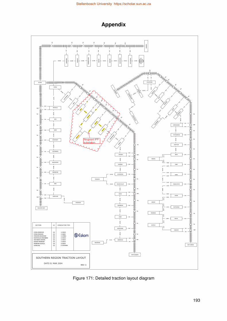
193
Appendix
Figure 171: Detailed traction layout diagram
NO
P
KA
RE
EB
OS
HP
AN
WIG
TO
N
32.56231.99934.00033.500
??
?
TS
S
TS
S
TS
S
TS
S
TS
S
TS
S
B-R
LALI
SA
DO
NKER
PO
OR
T
BESE
MB
OS
RU
IGTEV
ALLE
I
VALLEYDORA
STRYD
OM
STO
RM
BER
G
DREU
NBER
G
CARRICKMORE
PUTTERSKRAAL
LESSEYTON
BIRCH
CAMP
GAIKA
THOMAS RIVER
DOHNE
SOUTHDOWN
BERLIN
HIGHGATE
EAST LONDON
KOMANI
KUBUSIE
PEMBROKE
BUFFALO
TSS
TSS
TSS
NOP
8.715
26.919
20.574
27
.63
1
0.77
7
30.0
53
26.61
30
.39
3
21
.53
53
0.2
50
28
.69
4
26
.27
4.860
4.870
24
.54
01
6.7
60
20
.88
09
.46
16
.73
20
.30
11
.30
25
.73
6.1
21
.15
3.236
3.263
3.150
3.160
0.890
0.916
2.705
6.890
B-R
B-R
R-W
W-B
B-R
R-B
W-B
R-W
R-W
W-B
B-R
B-R
W-B
R-W
R-W
W-B
B-R
B-R
DE AAR
CRADOCK
DRENNAN
KLIPFONTEIN
GOLDON VALLEY
RIPON
DOORNKOM
VERBY
WOODLANDS
BRAKRIVIER
PORT ELIZABETH
TSS
TSS
TSS
TSS
TSS
TSS
TSS
TSS
38
.87
5
W-B
B-W
R-B
R-W
W-B
R-W
B-R
R-W
W-B
B-R
27
.14
9
POSEIDON
3.172
16.542
GRASSRIDGE
DROERIVIER
NOP
NOP
R-W
B-R
NOP
TSS
25
.96
23
0.2
51
28
.44
82
0.6
73
29
.67
63
9.2
98
ZWALL
UW
B-W
R-W
OLI
VE
29.841
25.095
TSS
NOP
DO
BBIN
GEN
OEG
SAAM
26.272
COLL
ETT
29.677
W-R
B-W
R-B
LUD
LOW
CARO
LUS
27.671
LIN
DE
30.802
R-B
W-B
R-B
TA
AIB
OS
BLE
TTER
MAN
30.933
R-W
B-W
NEW
GA
TE
30.487
R-W
22.2
74
0.010
TSS
TSS
TSS
TSS
TSS
TSS
TSS
TSS
TSS
NOP
TSS
TSS
TSS
TSS
CO
LESBERG
23.766
HYDRA
BRITSVILLE
15
.57
1
JOEN
28
.75
9
LAKEN
32
.12
4
BRAKPOORT
35
.15
9
HUTCHINSON
32
.27
0
BIESIESPOORT
23
.85
6
KROMRIVIER
33
.68
4
RIEM
26
.43
1
NORTH END
39
.33
2
W-B
R-W
B-R
W-B
R-W
R-B
R-W
B-W
R-B
W-B
BEAUFORT WEST
TSS
NOP
TSS
NOP
W-B
SOUTHERN REGION TRACTION LAYOUT
REV 3DATE:01 MAR 2004
KIM
BE
RLY
B-R
W-B
35.523
TS
S
KIM
BE
RLY
DIS
TR
IBU
TIO
N
ST
AT
ION
(KD
S)
SP
YT
FO
NT
EIN
BE
HR
SH
OE
K
KLO
KFO
NT
EIN
KA
LKB
ULT
GR
AS
PA
N
11.46429.800
R-W B-R
R-W
W-B
HYDRA-KDS
SECTION kV CONDUCTOR TYPE
HYDRA-DROERIVER
HYDRA-POSEIDON
POSEIDON-GRASSRIDGE
RUIGTEVALLEI-DREUNBERG
DREUNBERG-KOMANI
KOMANI-PEMBROKE
PEMBROKE-BUFFALO
132
132
220
1 X WOLF
132
132
132
132
1 X BEAR
1 X ZEBRA
1 X WOLF
1 X CHICADEE
1 X WOLF
2 X BEAR
132
1 X WOLF
15
.14
7
28.460
30.933
TSS
TSS
TSS
TSS
TSS
TSS
TSS
TSS
TSS
TSS
TSS
TSS27.671
CARO
LUS
LUD
LOW
30.802
R-
LIN
DE
0.010
-W
22.2
74
COLL
ETT
Noupoort IPPsubstation
NE
E
EWG
ATE
Stellenbosch University https://scholar.sun.ac.za

194
Figure 172: ABB inverter module drawing
Figure 173: Nameplate of the ABB inverter module
Stellenbosch University https://scholar.sun.ac.za

195
Figure 174: Nameplate of traction transformer
Stellenbosch University https://scholar.sun.ac.za