DYNAMIC MODELING AND SIMULATION OF FROST AND DEFROST CONDITIONS FOR

REFRIGERATION SYSTEMS

BY

LINDSEY M GONZALES

THESIS

Submitted in partial fulfillment of the requirements

for the degree of Master of Science in Mechanical Engineering

in the Graduate College of the

University of Illinois at Urbana-Champaign, 2015

Urbana, Illinois

Adviser:

Professor Andrew Alleyne

ii

Abstract

Heating and cooling systems are widely used throughout the world in an array of applications as a

means of providing thermal energy transfer. Recent decades have seen economic and environmental

awareness come to a forefront and innovation resultingly being pushed toward a standard of greater

performance and efficiency. With their nearly universal presence, it therefore comes as no surprise that

heating and cooling systems have also been subject to such guidelines. One of the biggest contributors to

performance degradation and inefficiency in air conditioning and refrigeration applications today is the

accumulation of frost on heat exchanger surfaces. The presence of frost often incurs a decrease in the

amount of cooling capacity achievable, resulting in the need for defrost cycles. Much work has been done

to date to establish strategies aimed at improving defrost decision making and allow for improved

operational efficiency. Nonetheless, some of the most common methods still permit defrost to run when

unnecessary. Modeling has therefore been used to provide greater insight and prediction capability of these

processes. However, current methods lack the qualities necessary to allow for the implementation of a

model-based defrost strategy aimed at further improving upon existing defrost techniques.

This thesis makes contributions toward improving refrigeration operational efficiency through the

development of a model for dynamically simulating refrigeration systems operating under both frost and

defrost conditions. Modeling provides the tools necessary to form more accurate defrost decisions through

a greater understanding of frosting behavior and its effect on system performance. Such insight is achieved

by means of developed frost growth and melt models discussed in the first part of this thesis. Validation

results demonstrate good prediction capability of both frost thickness as a function of time and estimated

time to defrost. The second portion of this thesis addresses implementation of frost growth/melt modeling

into an existing air conditioning and refrigeration simulation library. Coupling of frost and evaporator

dynamics under operation in cooling and defrost could therefore be represented; something existing models

do not allow for. Simulation results indicate that identified trends in system degradation are consistent with

those commonly seen in application. Agreement demonstrates the promise shown by developed models

and the potential utility of such a tool in aiding defrost decision making and further mitigating key

inefficiencies commonly plaguing the refrigeration industry today.

iii

To my family

iv

Acknowledgments

Though words cannot truly express my gratitude, I would like to take a moment to thank those whose

support and guidance over the past two years have made this thesis possible. First, I would like to thank

Dr. Alleyne for giving me the freedom to make decisions, but even more so for being there to provide

advice when I needed it. I genuinely feel that the guidance he has given on both an academic and personal

level has allowed me to walk away from this experience as an all-around better person. Additionally, I

would like to thank him for giving me the opportunity to join the Alleyne Research Group (ARG). I have

been extremely fortunate to have had the chance to work with such great and talented group of people and

in such a supportive environment. My experience would definitely not have been complete without all of

the current and former ARG members that I have had the pleasure to work with. Their advice and feedback

over the past two years has been invaluable in making this thesis a success.

The research conducted for this thesis was funded by the Air Conditioning and Refrigeration Center at

the University of Illinois at Urbana-Champaign and would not have been possible if not for their support.

I would also like to thank to the University of Illinois at Urbana-Champaign, Los Alamos National

Laboratory, and the National GEM Consortium for sponsoring me as a GEM Fellow. Without their support,

my goal of earning a Master’s degree would not have been attainable.

Last but certainly not least, I would like to express my appreciation to all of my family and friends who

have been there for me throughout the journey. To my parents who have spent countless hours helping me

move to and from school and whose support in all of my endeavors has been unwavering. Also, to my

sister whose friendship and ability to make me laugh have helped me get through many tough times. And

to my fiancé Andrew whose constant encouragement has helped me make it through some of even the most

stressful and challenging moments.

v

Table of Contents

LIST OF TABLES ................................................................................................................................ vii

LIST OF FIGURES ................................................................................................................................ ix

NOMENCLATURE ............................................................................................................................. xiii

CHAPTER 1 INTRODUCTION............................................................................................................ 1

1.1 Vapor Compression Cycles ........................................................................................................... 1

1.2 Defrost Cycles .............................................................................................................................. 4

1.3 Literature Review ......................................................................................................................... 6

1.4 Thesis Objectives ........................................................................................................................ 15

1.5 Thesis Outline ............................................................................................................................. 17

CHAPTER 2 MODELING .................................................................................................................. 18

2.1 Frost Growth ............................................................................................................................... 18

2.2 Frost Melt ................................................................................................................................... 25

CHAPTER 3 MODEL VALIDATION ............................................................................................... 53

3.1 Frost Growth ............................................................................................................................... 53

3.2 Frost Melt ................................................................................................................................... 56

CHAPTER 4 THERMOSYS™ IMPLEMENTATION .......................................................................... 62

4.1 Thermosys™ Overview .............................................................................................................. 62

4.2 Frost Growth Model .................................................................................................................... 63

4.3 Frost Melt Model ........................................................................................................................ 66

4.4 Finite Volume Evaporator ........................................................................................................... 71

4.5 Full Vapor Compression Cycle Implementation .......................................................................... 81

4.6 Conclusion ................................................................................................................................ 100

vi

CHAPTER 5 CONCLUSION ............................................................................................................ 102

5.1 Summary .................................................................................................................................. 102

5.2 Future Work ............................................................................................................................. 103

APPENDIX A: FROST GROWTH CORRELATIONS ....................................................................... 106

APPENDIX B: PRELIMINARY MELT MODELING ........................................................................ 109

APPENDIX C: FINNED MELT MODEL ........................................................................................... 113

APPENDIX D: EVAPORATOR SIMULINK BLOCK ........................................................................ 115

APPENDIX E: FULL CYCLE DATA FILTERING ............................................................................ 120

LIST OF REFERENCES ..................................................................................................................... 126

vii

List of Tables

Table 1.1: Frost Growth Studies .............................................................................................................. 8

Table 1.2: Published Modeling Summary .............................................................................................. 14

Table 1.3: Thesis Contributions ............................................................................................................. 16

Table 2.1: Coefficient Estimation Validity Range .................................................................................. 22

Table 2.2: Coefficient Estimation Heat Exchanger Specifications .......................................................... 22

Table 2.3: Nodal Phase Combinations.................................................................................................... 28

Table 2.4: Crank-Nicolson Notation ...................................................................................................... 29

Table 2.5: Nodal Element Study ............................................................................................................ 34

Table 2.6: Frost Melt Sensitivity Analysis ............................................................................................. 50

Table 3.1: Imeco Evaporator Specifications [16] .................................................................................... 57

Table 3.2: Frost Properties and Freezer Conditions [16] ......................................................................... 57

Table 4.1: Cooling Cycle Operating Conditions ..................................................................................... 81

Table 4.2: Full Cycle Implementation Model Comparison .................................................................... 85

Table 4.3: Frost Growth Sensitivity Analysis ......................................................................................... 91

Table 4.4: Hot-Gas Defrost Operating Conditions .................................................................................. 93

Table B.1: Intermediate Node Energy Balance Coefficients ................................................................. 109

Table B.2: Coil-Side Boundary Energy Balance Coefficients ............................................................... 110

Table B.3: Air-Side Boundary Energy Balance Coefficients ................................................................ 111

Table C.1: Water, Frost and Coil Properties ......................................................................................... 113

Table C.2: Time to Defrost by Frost Density ........................................................................................ 113

Table C.3: Time to Defrost by Frost Heat Capacity .............................................................................. 113

Table C.4: Time to Defrost by Frost Thickness .................................................................................... 113

Table C.5: Time to Defrost by Coil Diameter ....................................................................................... 113

Table C.6: Time to Defrost by Number of Fins .................................................................................... 114

Table C.7: Time to Defrost by Fin Thickness ....................................................................................... 114

Table C.8: Time to Defrost by Fin Thermal Conductivity .................................................................... 114

viii

Table C.9: Time to Defrost by Temperature ......................................................................................... 114

Table D.1: Standalone Frosted Evaporator Simulink Results (300 Fins) ............................................... 118

Table D.2: Standalone Frosted Evaporator Simulink Results (500 Fins) ............................................... 118

Table D.3: Standalone Frosted Evaporator Simulink Results (700 Fins) ............................................... 119

ix

List of Figures

Figure 1.1: Carnot Cycle.......................................................................................................................... 2

Figure 1.2: Vapor Compression Cycle ..................................................................................................... 2

Figure 1.3: Ideal Vapor Compression Cycle ............................................................................................. 3

Figure 2.1: Frost Growth Mass Transfer ................................................................................................ 19

Figure 2.2: Frost Growth Block Diagram ............................................................................................... 20

Figure 2.3: Frost Thickness vs. Time for Varying Fin Spacing ............................................................... 23

Figure 2.4: Frost Thickness vs. Time for Varying Air Velocity .............................................................. 24

Figure 2.5: Frost Thickness vs. Time for Varying Dew Point to Surface Temperature Difference ........... 24

Figure 2.6: Frost Volumetric Grid System ............................................................................................. 26

Figure 2.7: Preliminary Model Volumetric Energy Balance ................................................................... 27

Figure 2.8: Phase (left) and Enthalpy (right) vs. Time ............................................................................ 33

Figure 2.9: Predicted Time to Defrost vs. Number of Elements .............................................................. 35

Figure 2.10: Percent Prediction Time Change vs. Number of Elements .................................................. 35

Figure 2.11: Annular Fin ....................................................................................................................... 37

Figure 2.12: Finned Model Volumetric Energy Balance ......................................................................... 39

Figure 2.13: Simplified Thermal System Block Diagram ....................................................................... 40

Figure 2.14: Simulink Frost Melt Property Study Block ......................................................................... 41

Figure 2.15: Parameter Entry Tabs ......................................................................................................... 42

Figure 2.16: Enthalpy (top left), Temperature (top right), and Phase (bottom) vs. Time .......................... 42

Figure 2.17: Time to Defrost vs. Density ............................................................................................... 43

Figure 2.18: Time to Defrost vs. Heat Capacity...................................................................................... 44

Figure 2.19: Time to Defrost vs. Frost Thickness ................................................................................... 45

Figure 2.20: Time to Defrost vs. Coil Diameter...................................................................................... 46

Figure 2.21: Time to Defrost vs. Fin Pitch ............................................................................................. 46

Figure 2.22: Time to Defrost vs. Fin Thickness ...................................................................................... 47

Figure 2.23: Time to Defrost vs. Fin Thermal Conductivity ................................................................... 48

x

Figure 2.24: Time to Defrost vs. Coil Temperature ................................................................................ 49

Figure 2.25: Time to Defrost vs. Air Temperature .................................................................................. 49

Figure 2.26: Normalized Percent Time Change Magnitude and Direction by Parameter ......................... 51

Figure 2.27: Normalized Percent Time Change Magnitude by Parameter ............................................... 51

Figure 3.1: Frost Thickness vs. Time by Fin Spacing Comparison.......................................................... 54

Figure 3.2: Frost Thickness vs. Time by Air Velocity Comparison ......................................................... 54

Figure 3.3: Frost Thickness vs. Time by Temperature Difference Comparison ....................................... 55

Figure 3.4: Hoffenbecker Validation Simulink Block ............................................................................. 58

Figure 3.5: Hoffenbecker Validation Parameter Entry Tabs.................................................................... 59

Figure 3.6: Experimental (Hoffenbecker [16]) vs. Simulation Results .................................................... 60

Figure 4.1: Frost Growth Simulink Block .............................................................................................. 63

Figure 4.2: Frost Growth Simulink Block Ambient Conditions Entry Tabs ............................................ 64

Figure 4.3: Frost Growth Simulink Block Elements Entry Tab ............................................................... 64

Figure 4.4: Frost Growth Simulink Block Standalone Example .............................................................. 65

Figure 4.5: Simulated Frost Growth Frost Thickness vs. Time ............................................................... 65

Figure 4.6: Frost Melt Simulink Block ................................................................................................... 66

Figure 4.7: Frost Melt Simulink Block Frost Properties Entry Tab ......................................................... 67

Figure 4.8: Frost Melt Simulink Block Liquid Properties Entry Tab ....................................................... 68

Figure 4.9: Frost Melt Simulink Block Heat Exchanger Properties Entry Tab......................................... 68

Figure 4.10: Frost Melt Simulink Block Elements Entry Tab ................................................................. 69

Figure 4.11: Frost Example Simulink Block Standalone Example .......................................................... 70

Figure 4.12: Simulated Frost Melt Enthalpy (top left), Temperature (top right), Phase (lower left), and Frost

Thickness (lower right) vs. Time ........................................................................................................... 71

Figure 4.13: Finite Volume Evaporator Simulink Block ......................................................................... 72

Figure 4.14: Frosted Finite Volume Evaporator Simulink Block ............................................................ 75

Figure 4.15: Frosted Finite Volume Evaporator Simulink Block Evaporator Geometry Entry Tab .......... 76

Figure 4.16: Frosted Finite Volume Evaporator Simulink Block Evaporator Geometry Entry Tab .......... 77

Figure 4.17: Evaporator Cooling Capacity vs. Frost Thickness ............................................................... 78

Figure 4.18: Evaporator Air Outlet Temperature vs. Frost Thickness ..................................................... 79

Figure 4.19: Evaporator Refrigerant Outlet Temperature vs. Frost Thickness ......................................... 79

Figure 4.20: Refrigerant Outlet Pressure vs. Frost Thickness.................................................................. 80

Figure 4.21: Cooling Cycle Simulink Schematic .................................................................................... 82

Figure 4.22: Full Cycle Frost Finite Volume Evaporator Simulink Block ............................................... 83

Figure 4.23: Full Cycle Frost Growth Simulink Block ........................................................................... 84

xi

Figure 4.24: Cooling Baseline Evaporator Wall Temperature vs. Time .................................................. 86

Figure 4.25: Cooling Finned Unfrosted Evaporator Wall Temperature vs. Time ..................................... 86

Figure 4.26: Cooling Frosted Evaporator Wall Temperature vs. Time .................................................... 87

Figure 4.27: Cooling Cycle Cooling Capacity vs. Time (Filtered) .......................................................... 88

Figure 4.28: Cooling Cycle Air Outlet Temperature vs. Time (Filtered) ................................................. 89

Figure 4.29: Full Cycle Refrigerant Outlet Temperature vs. Time .......................................................... 90

Figure 4.30: Cooling Cycle Refrigerant Outlet Pressure vs. Time ........................................................... 90

Figure 4.31: Normalized Percent Cooling Capacity Change Magnitude by Parameter ............................ 92

Figure 4.32: Hot-Gas Defrost Simulink Schematic ................................................................................. 94

Figure 4.33: Defrost Cycle Frost Melt Simulink Block ........................................................................... 95

Figure 4.34: Defrost Baseline Evaporator Wall Temperature vs. Time ................................................... 96

Figure 4.35: Defrost Finned Unfrosted Evaporator Wall Temperature vs. Time ...................................... 97

Figure 4.36: Defrost Frosted Evaporator Wall Temperature vs. Time ..................................................... 98

Figure 4.37: Defrost Cycle Heating Capacity vs. Time (Filtered) ........................................................... 98

Figure A.1: Fin Pitch Coefficient 1 ...................................................................................................... 106

Figure A.2: Fin Pitch Coefficient 2 ...................................................................................................... 106

Figure A.3: Velocity Coefficient 1 ....................................................................................................... 107

Figure A.4: Velocity Coefficient 2 ....................................................................................................... 107

Figure A.5: Temperature Difference Coefficient 1 ............................................................................... 108

Figure A.6: Temperature Difference Coefficient 2 ............................................................................... 108

Figure D.1: Finite Volume Evaporator Simulink Block Evaporator Geometry Entry Tab ..................... 115

Figure D.2: Finite Volume Evaporator Simulink Block Wall Properties Entry Tab ............................... 116

Figure D.3: Finite Volume Evaporator Simulink Block Parameter Adjustment Factors Entry Tab ........ 116

Figure D.4: Finite Volume Evaporator Simulink Block Refrigerant/Air Properties Entry Tab............... 117

Figure D.5: Finite Volume Evaporator Simulink Block Initial Conditions Entry Tab ............................ 117

Figure D.6: Finite Volume Evaporator Simulink Block Simulation Entry Tab ...................................... 118

Figure E.1: Butterworth Filter Simulink Block ..................................................................................... 120

Figure E.2: Butterworth Filter Block Inputs ......................................................................................... 120

Figure E.3: Cooling Cycle Cooling Capacity vs. Time (Unfiltered) ...................................................... 121

Figure E.4: Filtered vs. Unfiltered Cooling Cycle Cooling Capacity ..................................................... 121

Figure E.5: Filtered vs. Unfiltered Cooling Cycle Cooling Capacity (Zoomed) .................................... 122

Figure E.6: Cooling Cycle Air Outlet Temperature vs. Time (Unfiltered) ............................................. 122

Figure E.7: Filtered vs. Unfiltered Air Outlet Temperature................................................................... 123

Figure E.8: Filtered vs. Unfiltered Air Outlet Temperature (Zoomed) .................................................. 123

xii

Figure E.9: Defrost Cycle Heating Capacity vs. Time (Unfiltered) ....................................................... 124

Figure E.10: Filtered vs. Unfiltered Defrost Cycle Heating Capacity .................................................... 124

Figure E.11: Filtered vs. Unfiltered Defrost Cycle Heating Capacity (Zoomed).................................... 125

xiii

Nomenclature

Symbols

A area [m2]

Atotal overall surface area (coil and fins) [m2]

C mass thermal capacity [kg]

c heat capacity [kJ/kg*K]

d diameter [m]

F frost

FP fin pitch

h enthalpy [kJ/kg]

hc heat transfer coefficient [kW/m*K]

hlat latent heat of fusion (334 [kJ/kg])

k thermal conductivity [kW/m*K]

L liquid or length [m]

N number of volumes

Nfin number of fins

Q rate of heat transfer [kW]

R outermost radial node location [m]

Rcond conductive thermal resistance [K/kW]

Rconv convective thermal resistance [K/kW]

RH relative humidity [-]

Ra air-side heat thermal resistance

Rc coil-side heat thermal resistance

r radial distance [m]

T temperature [K] or indicative of transition phase

t thickness [m]

xiv

V volume [m3] or velocity [m/s]

w previous node tridiagonal matrix coefficient

X quality or phase

y current node tridiagonal matrix coefficient

z next node tridiagonal matrix coefficient

α thermal diffusivity [m2/s]

ηf single fin efficiency [-]

ηo overall surface efficiency [-]

𝜌 density [kg/m3]

Δr width of element [m]

Δt timestep [sec]

Subscripts

air air property

coil coil, or base property

i-1 previous node location

i current node location

i+1 next node location

f frost property “also denoted as “frost”

l liquid

m melt

r inner radius

r+Δr outer radius

t coil or tube

V velocity

Superscripts

n-1 previous timestep

n current timestep

n+1 next timestep

1

Chapter 1

Introduction

Over the last several decades, energy conservation has played a significant role in influencing the drive

and direction of technological advancement. As fuel prices rise, awareness of environmental impact

increases, and resources head toward depletion, increased concerns regarding energy consumption have

created a drive toward greater energy efficiency in all aspects of life. Examples of this can be seen from

the integration of electric vehicles onto highways to energy efficient light bulbs in homes. Although

innovation has pushed researchers in the direction of greater efficiency, one area that has stood out as one

in most need of improvement is heating and cooling [4].

Heating and cooling systems are widely used in a multitude of applications to maintain spatial

temperatures ranging from human comfort to preventing food spoilage. It therefore comes as no surprise

that heating and cooling remains one of the world’s leading means of energy consumption, accounting for

nearly half of all energy usage. According to the US Department of Energy, “heating and cooling accounts

for about 48% of energy consumption in US homes” [14]. As prevalent as these applications are, it is

evident that even small scale improvements could greatly reduce energy consumption. As a result, it is

important that steps be taken to further improve operating conditions as a means of reducing both costs and

global energy consumption.

1.1 Vapor Compression Cycles

The most general cycle seen in thermodynamics is the Carnot Cycle, which can be seen in Figure 1.1.

The Carnot Cycle is an idealized cycle with operation between a low temperature region, TC, and a high

temperature region, TH. With the 2nd Law of Thermodynamics comes the concept of losses in

thermodynamic systems as a result of irreversibilities. The Carnot Cycle is a perfectly reversible system

which provides the highest achievable efficiency, consisting of the four key process indicated to the right

of Figure 1.1 [27]. Real systems are however incapable of operating without losses as the result of friction

or other such imperfections.

2

Figure 1.1: Carnot Cycle

One such system, is a vapor compression cycle. Vapor compression systems are commonly used in

applications where temperature control is desired. As in the Carnot Cycle, this is done by removing heat

from a low temperature region and expelling the heat into a higher temperature region. Vapor compression

cycles make use of thermodynamic phase change properties during evaporation and condensation to

replicate behaviors exhibited by the Carnot Cycle as a means of minimizing losses associated with

imperfections [27]. This is accomplished through the use of four major components, those being an

evaporator, a compressor, a condenser, and an expansion device, as seen in Figure 1.2.

Figure 1.2: Vapor Compression Cycle

Figure 1.3 displays an ideal vapor compression cycle, consisting of four processes. Those processes

are isentropic compression, isobaric heat rejection to a high temperature region, isenthalpic expansion, and

isobaric heat absorption from a region of low temperature. Lines of constant pressure coincide with those

3

of constant temperature during phase change, allowing vapor compression systems to emulate Carnot Cycle

operation within the vapor dome and further achieve maximum efficiency. This means that an isothermal

process (constant temperature) is achievable within the vapor dome by means of a constant pressure process

(isobaric).

Figure 1.3: Ideal Vapor Compression Cycle

System optimization can require significant knowledge into how each component operates, as well as

how the system as a whole will be affected as a result of various changes. In cycle configuration outlet

conditions of one component become input conditions of the next. This means that each component is

heavily reliant on the previous and that changes in the operation of one will subsequently affect the behavior

of each of the others.

1.1.1 Frost Accumulation

As phase change is critical to vapor compression system operation, it is important to discuss the means

by which this is achieved. A means of heat transfer is first needed to remove heat from a region of low

temperature (evaporator) and expel this heat to a region of high temperature (condenser). External fluids

can be used to remove/add heat to refrigerant flowing within the system piping by increasing heat transfer

surface area through the use of fins, grooves, or other surface manipulations. Refrigerants are commonly

designated as fluids with relatively low boiling point.

The most frequently used heat transfer medium to achieve this is air. Air has somewhat subpar heat

capacitive properties in contrast to alternatives such as water, but one major benefit is that operational costs

tend to be lower as a result of high availability and ease of flow manipulation. One of the biggest drawbacks

of air as a heat transfer medium is its capacity to carry moisture. Frost growth will ensue when the surface

4

temperature of the heat transfer surface drops below that of the dew point of the surrounding moist air as

well as the freezing point of water. Thickening layers of frost introduce a challenge for refrigeration system

operation with a resulting reduction in heat transfer.

1.2 Defrost Cycles

One of the most common problems encountered in the refrigeration industry today is the buildup of frost

on heat exchangers surfaces as a result of moist air being used as a heat transfer medium. Frost growth

often occurs due to the moisture content of the air as well as the generally low operating conditions of

evaporators. Studies have shown that frost growth initially enhances heat transfer with increased surface

area and turbulent air flow as a result of surface roughness associated with its crystalline structure [7].

However, layers of frost will start to act as insulation over time, inhibiting both heat transfer and air flow

through the system. This results in the ultimate reduction of cooling capacity ([3], [32]). With the reduction

in evaporator cooling capacity, desired environmental temperatures may become difficult or impossible to

maintain. Operation under these circumstances could be particularly detrimental in cases where tight

temperature tolerances are desired, such as in food storage applications. Frost accumulation could

ultimately cause system failure with the complete blockage of airflow through the system. Counteractive

measures in the form of defrost cycles must therefore be taken to allow system operation to resume as

necessary.

1.2.1 Defrost Methods

Various techniques have been developed as a means of employing defrost cycles for frost removal.

Among those are hot-gas, electric, off-cycle, water, and secondary fluid, for which Reindl et al. (2009) [31]

has provided an overview of advantages and disadvantage of each. Hot-gas defrost is one of the most

commonly applied methods of defrost in both industrial and commercial applications and will therefore

primarily be used for the purpose of this thesis. The hot-gas defrost process is conducted by routing hot,

compressed gas through the evaporator by means of a valve. This is in contrast to its usual path through

the condenser, which can be seen in Figure 1.2. The evaporator will behave more like a condenser under

operation in defrost, rejecting heat to the environment rather than removing it. Although hot-gas defrost

will be the focus of further discussion, it is likely that methods and modeling discussed in later sections are

highly applicable the other aforementioned defrost approaches. One example of this is electric defrost for

which a constant heat flux boundary condition is provided rather than temperature boundary condition.

1.2.2 Defrost on Demand vs. Timer-Based

In addition to having differing methods of achieving frost melt, there are similarly varying methods for

triggering of the defrost process. A review of many of these methods can be found in [11]. Two of the

5

most common techniques used in application are defrost on demand and timer-based. Defrost on demand

systems make use of gauges for measuring operating conditions, such as temperature drop or pressure drop

across the evaporator, to determine when defrost should be initiated. These systems tend to be more

efficient than some alternatives as these measurements provide some feedback to the system. However,

additional instrumentation necessary for obtaining such measurements causes these systems to also be more

costly upfront. Measurements are commonly only used to determine when defrost should be initiated, but

not necessarily to determine when the cycle should be terminated. This results in some circumstances in

which defrost is run in excess. Additionally, these systems are reactive in that certain conditions must be

met before defrost will be triggered.

Timer-based systems make use of set time periods of operation that are continually repeated. For

instance, a system may run in refrigeration for an extended period of time on the order of about 10 hours.

After that time period, a defrost cycle will run for a designated time period of about 10 min. As soon as

this 10 min defrost cycle is completed, the system will resume refrigeration for yet another 10 hours. This

cycle will then continue to repeat as long as the system continues to run or until timer settings are altered.

Although less costly upfront than a defrost on demand system, one of the major drawbacks of timer-based

systems is that operation is the same regardless of ambient conditions. This means that they must be

designed for operation under ‘worst case’ conditions, such as those in which relative humidity is on the

high end for the region in which the system is being run. As previously discussed, humidity is the biggest

contributor to frost development on evaporator surfaces. Air with high humidity has a higher dew point

temperature, as it does not require as much of a temperature drop before the air becomes saturated and

begins to produce dew. This means that when humidity levels are high, the capacity to develop frost is also

greater.

There is a higher potential that there may be a significant amount of frost present on a heat exchanger

after the refrigeration portion of the cycle has run in locations where humidity is relatively high (e.g.

Illinois). An identical system running in a region where humidity levels are generally low (e.g. New

Mexico) may not see any frost growth after the designated refrigeration period, yet still be required to run

a defrost cycle. A similar case can be presented for season to season operation in which humidity levels

tend to be higher during warmer months and lower during cooler ones. Timer settings should ideally be

changed routinely to account for such variations in location and season, but this often tends to be

overlooked. Additionally, continual switch between operation in cooling and in defrost, particularly when

unnecessary incurs a greater amount of wear and tear on system components.

6

1.2.3 Operational Effects

Despite being an integral part of maintaining system functionality, running of a defrost cycle does come

at some cost. Besides being unable to provide cooling capacity during defrost, the system actually adds

heat to the region being cooled. Although a fair amount of the energy provided during defrost goes into the

phase change process to melt and ultimately shed the layer of frost, some energy is actually conducted to

the surrounding air. As cited by Mohs (2013), “75% - 85% of the energy required to defrost the evaporator

coil is lost to the refrigerated space as a parasitic heat load” [26].

In addition to heat conduction through the frost layer, one major contributor to this heat loading and

decreased operational efficiency is defrost being run when unnecessary. This may come as a result of early

triggering or running in defrost beyond the timeframe in which frost is present, both of which are common

in defrost on demand and timer-based defrosting strategies frequently used in application today. Under

such circumstances, the refrigeration cycle will then have to compensate for excess heat being expelled to

the region being cooled. Therefore, efficiency could greatly be improved by simply being able to identify

more accurately when defrost initiation and termination should occur

1.3 Literature Review

As frost accumulation on heat exchanger surfaces has proved to be a major plague on the efficiency

associated with heating and cooling systems, significant research has gone into experimental research and

model development over the past several decades in order to gain a better understanding and prediction

capability of the growth and melt processes and their respective impact on system performance. Many

studies have been conducted as a means of determining how various parameters affect frost growth and the

extent to which they do so. Although fewer in number, various studies have also been aimed at determining

defrost time based on various parameters as well. An extensive amount of research in the area has been

conducted, so the following few sections will provide a brief overview of only some of the currently

published studies.

1.3.1 Frost Growth

Numerous studies over the past several decades have shown that varying ambient, operating, and

geometric conditions can greatly influence frost growth. In some cases, these studies were specific to flat

or cylindrical surfaces, however, more recent studies have started to focus more on fin-tube heat exchangers.

Due to the vast quantity of studies that have been conducted in this area, this section will only focus on a

few more recent ones.

Hermes et al. (2009) [15] studied the process of frost growth and densification on flat surfaces.

Experimentation was first conducted to gain a physical understanding of the frost growth process. This

7

greater physical knowledge in addition to energy and mass balance equations then served as a basis for

model development. Experimental work was broken into two sets. The first set consisted of 14 experiments

in which air velocity (0.7 m/s to 1 m/s), air relative humidity (50% to 80%), inlet air temperature (16 ˚C to

22˚C), and plate surface temperature (-18˚C to -5˚C) were varied to identify the influence of each on frost

thickness. A total of 12 experiments were conducted in the second set to evaluate the designated impact on

frost densification. Air velocity was held constant at 0.7 m/s and plate surface temperature was kept

between -5˚C to -15˚C. Otherwise, all parameter ranges were identical. Results indicate that frost thickness

was higher for cases in which surfaces temperatures were lower. However, air velocity was seemingly

found to have little to no impact on growth. Modeling showed good prediction capability with agreement

lying between +/-10%.

Wang et al. (2012) [36] conducted a similar study composed of both experimental and modeling parts

however, parameter ranges differed somewhat. Air temperatures was instead kept between -8˚C and 19˚C,

surface temperatures between -16˚C and -8˚C, relative humidity between 45% and 80%, and air velocity

between 0 m/s and 9 m/s. Modeling predictions were made and frost thickness results validated against

collected and published experimental results. Findings show that frost thickness was greater when surface

temperature were lower, humidity levels were higher and air temperature was higher. The majority of

model predictions proved to agree with experimental finding with an average deviation of +/-8% and

maximum error of +/-12

Additional studies have gone on to look into the effect various parameters have on frost accumulation

on cylindrical surfaces. Lee et al. (2001) [22] conducted experiments with variables being air temperature,

humidity, and air flow rate. The surface temperature of the cylinder was maintained at a constant

temperature of -17˚C. Frost thickness measurements were then taken at 90˚ from one another to determine

how frost growth is distributed along cylindrical surfaces. Findings indicate that higher humidity ratio

correlated to a greater potential for mass transfer and results in a relatively thicker layering of frost after a

given period of time. Though having a much lesser effect, higher air temperature also corresponded to

thicker frost.

Much of the research in this area has been the result of the negative impact frost accumulation has

incurred on the refrigeration industry. It therefore comes as no surprise that more recent efforts have

focused on the frost growth process associated with heat exchanger geometry. One such study was

conducted by Lee et al. (1996) [23] in which experimental testing was used to evaluate the effect of fin

spacing, fin arrangement, air temperature, air humidity, and air velocity on the frost growth and thermal

performance of a finned-tube heat exchanger. Fin spacings ranged between 5 mm and 20 mm, with findings

showing that frost thickness increased with greater fin spacing. Increased air velocity showed a similar

relationship to frost thickness. Trends for all other parameters were similar to those of the aforementioned

8

studies in which higher humidity levels and air temperature resulted in a greater amount of frost

accumulation after a 200 min test run.

Cui et al. (2011) ([5] and [6]) developed a theoretical representation of frost growth on a finned-tube

heat exchanger. In addition to model development, test cases were used to determine the influence of

various parameters on frosting behavior and the resulting heat transfer coefficient. Parameters of interest

included fin pitch, relative humidity, air velocity, and evaporator surface temperature. Increased frost

thickness was found to correspond to decreased fin pitch, decreased air velocity, increased relative

humidity, and decreased evaporator surface temperature. Validation efforts determined a maximum error

of 13% between predicted values and those of published experimental findings after a 6 hour timeframe.

One of the biggest benefits of this model in contrast to many of those previously mentioned is that frost

growth was allowed to run over a timeframe closer to those commonly seen during refrigeration operation.

Many of the aforementioned studies were only allowed to run for about one to three hours.

A summary of these studies has been provided in Table 1.1 to provide a better visualization of the

contributions of each of the aforementioned frost growth studies. The top row designates the study type,

geometry, and parameters that were considered in the study. For instance, Lee et al. experimental findings

for fin-tube heat exchangers for variances in air temperature, humidity, air velocity, and fin spacing.

Table 1.1: Frost Growth Studies

Study

Type Geometry

Air

Temperature

Surface

Temperature Humidity

Air

Velocity

Fin

Spacing

Lee et al.

(1996) Experiment

Fin-Tube

HX X X X X

Lee et al.

(2001) Experiment

Cylindrical

Tube X X X

Hermes et

al. (2009)

Model and

Experiment Flat Plate X X X X

Cui et al.

(2011) Model

Fin-Tube

HX X X X X

Wang et al.

(2012) Model Flat Plate X X X X

In all of the aforementioned cases, findings show that frost growth is most rapid in early stages of frost

growth and decreases as time progresses. Another common finding is that frost accumulation increases

with increased air temperature, air velocity, and relative humidity. This was also true for decreased

refrigerant or evaporator surface temperature. In regard to heat exchanger geometry, Cui et al. found that

the amount frost buildup after a given period of time increased with decreased fin pitch. Lee et al. found

that the opposite was true. As this has been a widely studied field with many published works, it is not

9

uncommon for various studies to have somewhat contradictory findings. This could be due to various

factors, including variations in geometry upon which experiments and models are based.

In addition to the above studies, Iragorry et al. (2004) [19] provides a literature review of several

decades worth of experimental findings as well as numerical and analytical models that have been aimed at

predicting frost growth behavior. Included is/are some theoretical background on the stages of frost

formation, property correlations (e.g. thermal conductivity, density, frost thickness) for various geometries,

as well as various modeling approaches that have been implemented in past works as a means of setting the

groundwork for future efforts.

1.3.2 Frost Effects on System Operation

Although there has been a long history of research in the area of frost growth and its effect on heat

transfer, the following review will focus more on recent studies and their findings, specifically those relating

to finned-tube heat exchangers. Among those within the last few decades is Ali (1992) [1]. His research

focused on studying the effect of frost on evaporator surfaces as a result of varying volumetric air flow rate

and fin pitch. This was accomplished by conducting two studies. In the first, a fin pitch of 5 fins per inch

was used, with air flow rates ranging from 20 cfm to 70 cfm. Similarly, a study was conducted for a 2.5

fins per inch case, in which flow rates were allowed to vary between 40 cfm and 80 cfm. For both cases,

frost was then allowed to build over the course of 10 hours. Findings show that there is an increase in heat

transfer with an increased presence of frost, attributed to increased surface area and local air velocity.

Pressure drop across the evaporator showed an increase with more frost buildup, particularly for cases in

which a higher air flow rate was used. Variations in fin pitch show that the overall heat transfer coefficient

was proportionally larger to increases in surface area (greater number of fins per inch). However, the rate

of frost deposition did not show the same correlation. Findings showed that for an increased number of

fins per inch (lower fin pitch), the amount of accumulated frost mass was generally lower. One of the

suggestions made for improving this study by the author was to run the system under higher frosting rates

due partly to the fact that the insulation effect associated with frost accumulation was not seen.

Kondepudi and O’Neal (1993) conducted a two-phase study in which a model was created to represent

the effect frost growth has on finned-tube heat exchanger performance ([20], [21]). Evaporator surface area

was broken up into finite volumes to evaluate various parameters over differing sections of the coil.

Parameters of interest in this study were frost height, energy transfer, and pressure drop across the

evaporator. In the second phase, experiments were conducted for validation purposes, with findings

showing that modeling under predicts both frost growth and airside pressure drop. The model showed good

predicting capability for the energy transfer coefficient, with a difference of about 15% to 20%. An

10

improved model representation was developed by Tso et al. (2005) [34], bringing results within about 0.8%

of experimental values. Model predictions showed relatively good alignment with behavior under

experimental conditions in all cases, with slight deviations being visible between experimental data and

model predictions toward the end of the 50 min run time. As refrigeration cycles generally run for time

periods on the order of hours, these predictions may not hold up quite as well under longer time frames

more characteristic of cooling applications.

Yan et al. (2003) [39] also went on to perform experimental studies on the effects of various parameters,

including humidity levels (60%, 70%, and 80%,), air temperature (2.5°C, 5°C, and 7.5°C) and flow rate (12

m3/min, 24 m3/min, and 36 m3/min), refrigerant temperature (10°C and 15°C), row number, and fin pitch

(1.6 mm, 1.8 mm, and 2 mm). These parameters were used to evaluate the effect of each on the rate of heat

transfer, overall heat transfer coefficient, and pressure drop across the heat exchanger [39]. Findings

indicate that the rate of heat transfer decreased with decreased air flow rate, increased air and refrigerant

temperature, and increased relative humidity. It is also noted that lower surface temperatures resulting from

decreased air flow caused an increase in the amount of frost growth. Fin pitch, however, exhibited relatively

low effect on performance. This could be the result of such a small range of fin pitch distance, as there was

only a total change of 0.4 mm. One thing that is important to note is that despite all of the work that has

been done to date to better comprehend the behavior of frost and its effects, there have been many instances

where studies have found contradictory results. Yan et al. in fact notes that some of their findings differ

from other previously published studies.

With many past studies focusing on experimental analysis, Yang et al. (2006) [40] developed a

numerical model for predicting behavior of fin-tube heat exchangers operating under frosting conditions to

meet demand for such capability. Heat transfer coefficients were established by combining findings of

experimentally found correlations associated with both cylindrical surfaces and cold plates, resulting in

modeling being broken up into two parts. Numerical findings were validated with experimental data,

indicating good agreement in parameters such as average frost thickness, rate of heat transfer, and frost

mass.

Various methods have also been developed to evaluate the efficiency of heat exchangers as a result of

frosting conditions. Xia and Jacobi (2004) [37] developed an exact solution for conduction on a one

dimensional fin, with further work done by Sommers and Jacobi (2006) [33] to provide a similar solution

for circular fins. Similar analytical analyses have been conducted to evaluate fin efficiency for composite

fins. As a frosted fin can be considered a composite surface consisting of both fin material and frost, many

of these studies are also relevant. Tu et al. (2006) [35], for instance, provides various analytical

11

representations for composite fins of differing make up, covering cases in which thermal conductivity of

the fin coating is much less, equivalent, or greater than that of the coating material.

1.3.3 Frost Melt

Although frost growth is the primary cause of inefficiency associated with refrigeration operation,

another very important aspect of understanding the overall process includes a greater comprehension of the

frost melt process as well. Consequently, similar efforts have gone into developing a greater knowledge

and modeling capability to represent the melt process during system defrost.

Alebrahim and Sherif (2002) [1] make use of the enthalpy method in tracking phase change throughout

the defrost process in order to determine how long defrost must last to remove the accumulated layer of

frost. For this study, annular fins were focused on, with a constant heat flux being provided for defrost.

However, it is suggested that slight modifications can be made to support analysis for different types of

systems and defrost operation as well. It is assumed that a uniform layer of frost has built up on the finned

surface for initial conditions, which is then broken up into a number of elements. Finite differencing

methods are used to iteratively evaluate enthalpy for each nodal region at each timestep, thus providing

insight into how much of the frost layer has melted at any point in time. It should be noted that the model

is not validated, nor is there any discussion on modeling accuracy. Findings do, however, support past

study findings in that the time to defrost decreases as the amount of heat flux increases.

Hoffenbecker (2004) [16] and Hoffenbecker et al. (2005) [17] developed a model for simulating frost

melt under hot-gas defrost conditions for a heat exchanger with annular fins. By assuming an initially

uniform layer of frost growth on the fin surface, the model takes advantage of radial symmetry in the

development of a finite volume approach to evaluating the melt process by means of nodal energy balances.

It is interesting to note that this model does not take into account the mass of frost buildup on the coil

surface as well. Instead, frost thickness was based solely on the frost accumulation on the finned surface,

and is estimated as a blockage percentage based on how much of the fin spacing gap is obstructed. Overall,

the model shows decent predicting capabilities with estimated defrost lasting 10 min and 45 sec, while

qualitative analysis of the experimental system used for validation shows that a 10 min to 14 min timeframe

was necessary to fully remove the accumulated layer of frost. The model was then used to estimate the

parasitic loading under various defrost operating conditions to identify optimum operating conditions.

These optimal operating conditions are defined as those which would minimize the loading associated with

defrost. One drawback of this model, however, is that the fin base temperature remains constant. In reality,

fluctuations in the rate of frost melt may be present as a result of potentially transient surface temperatures

that are not accounted for here.

12

Similar to the work done by Hoffenbecker, Dopazo et al. (2010) [9] created a hot-gas defrost model

representation, in which energy balances are broken up into a series of system relations, such as refrigerant,

tube, fin, frost, etc. All of these systems are interconnected such that changes in one propagate through the

remaining systems. Here, it is also worth noting that defrost is considered to go through a series of six

stages in total. These stages consist of preheating, tube frost melt, fin frost melt, air presence, tube-fin,

water film, and dry-heating. Energy balance equations, thus, change from stage to stage to account for

varying physical properties. Finite differencing was used for evaluating various system properties at each

timestep. Model validation was then conducted by two means. First, experimental tests were run on a

physical system for comparison against model results. Second, data provided in Hoffenbecker (2004) was

also utilized for comparison. Modeling produced an estimated defrost time of 14 min and 3 sec, while a

qualitative experimental defrost time was estimated at 15 min. The model also displayed good prediction

capability with about 2.5% less error than that found by Hoffenbecker.

Mohs (2013) developed a model aimed at representing frost melt on a vertical surface during defrost,

for further implementation as a vertical plain fin. Where many past studies have focused on the heat transfer

aspect of defrost, this study also looked at mass transfer and its effect on the melt process. Since frost is a

porous medium, understanding how mass is transferred both within the layer and to the environment can

be critical to gaining a greater knowledge of the melt process overall. To fully comprehend this behavior

throughout the defrost process, analysis was conducted to account for behavior through all stages of defrost

(pre-heat, melt, dry-out, and re-cool). For validation purposes, experiments were conducted in which frost

was initially grown on a vertical Peltier plate in order to obtain an estimate for the initial conditions of the

defrost process. Constant heat flux was then delivered to the layer to simulate defrost. Despite under

predicting defrost duration time in all three stages of defrost, overall, the model provided favorable results,

as it was able to predict defrost time within about 20% of experimentally measured values. One drawback

of the model, however, is that although it does provide greater insight into the behavior of the frost layer

during defrost, it was found to be too complex and time consuming for implementation in a full scale heat

exchanger model. Instead, a full heat exchanger model was developed with individual fin effects somewhat

passive in order to cut down on simulation time. Recommendations for future work involve including the

effect of fin efficiency, as this was meant to solely represent a vertical surface (single fin). Additionally, a

“dynamic frosted-defrosted heat exchanger model” is suggested to allow for improved overall system

efficiency.

1.3.4 Defrost Effects on System Operation

Unlike for the frosting case, for which most research has gone toward evaluating effects on evaporator

operating conditions, most studies regarding defrost have had a greater focus on environmental and expense

13

effects. More importance has been placed on measuring the resulting parasitic loading contributed to the

environment as well as additional costs associated with the defrost process. For instance, Hoffenbecker

(2004) [16] used modeling of the defrost phenomena to determine optimal defrost operating conditions in

order to minimize the effect of loading. Other studies have examined the division of how much defrost

energy is contributed to individual components as a result of variations in defrost. This includes how much

energy goes to phase change as well as how much of that thermal energy is being contributed to the

environment as a parasitic load. Nelson (2011) [29] provides an overview of some parameters found to

affect this breakdown, including room temperature, hot-gas temperature, defrost duration, frost thickness,

and heat exchanger material.

Liu et al. (2003) [23] provides an experimentally validated mathematical representation of air-source

heat pump transients during the early stages of hot-gas defrost. Findings indicate trends in suction and

discharge pressure, inlet and outlet temperatures, and compressor work as a function of time for the first

three minutes of both simulation and experimentation. Estimates of both transient behaviors of evaporator

operation as well as defrost time show decent correlation with experimental findings, with defrost

estimations differing by only about 8%. Besides analysis of initial transients associated with startup of

defrost, other studies have also looked into the effect of cyclic behavior of alternating between refrigeration

and defrost cycles. On such study was conducted by Xia et al. (2006) [38]. Findings indicate a decrease

in overall heat transfer coefficient, however, there is an increase in defrost efficiency after a few cycles.

This is attributed to higher initial temperatures at the start of defrost, which may inhibit frost growth.

Another interesting finding based on studies conducted by Muehlbauer (2006) [28] is that after several

cycles, more frost growth tends to occur, potentially due to run-off refreezing on evaporator surfaces. This

could also contribute to improved defrost efficiency during later cycles, as findings have shown that greater

efficiency is generally seen when the frost layer is more dense.

1.3.5 Summary

The literature review discussed in previous sections briefly details some of the studies conducted over

the past few decades on evaporators operating under frosting conditions. These works demonstrate the

tireless research that has gone toward obtaining a firmer grasp and modeling capability of frost behavior

and its impact on refrigeration system operation. Some studies have focused on determining the effect that

various parameters have on the frost growth process, whereas others have been aimed at identifying

operational effects associated with such growth. Although seemingly fewer, numerous studies have also

concentrated on understanding the heat and mass transfer phenomena characteristic of the frost melt

process. As inefficiency and cost associated with such are the primary cause for much of this research, a

significant amount of work has also gone into quantifying these said losses. Through this quantification,

14

studies have also gone on further to provide suggestions aimed at optimizing defrost processes. Modeling

efforts detailed in previous sections have been summarized in Table 1.2. Despite how much the knowledge

base regarding refrigeration systems operating under frosting conditions has evolved, there still exist some

areas in need of improvement.

Table 1.2: Published Modeling Summary

Frost Growth Frost Melt Coupled Behavior Transient

Kondepudi et al. (1993) X X X Alebrahim and Sherif (2002) X X

Hoffenbecker (2004, 2005) X X

Tso et al. (2005) X X X Yang et al. (2006) X X X

Hermes et al. (2009) X Dopazo et al. (2010) X X X

Cui et al. (2011) X Wang et al. (2012) X

To the author’s knowledge, there is no current model that allows for the dynamic simulation of the

coupling between evaporator conditions and frost behavior under both modes of operation (refrigeration

and defrost). This can be seen in Table 1.2 above, in which no single study has all of the designated

characteristics. Many models, including that presented by Hoffenbecker, do not allow temperature

conditions to be transient and call for environmental and system conditions to be constant throughout the

simulation. Models are also generally either aimed at predicting frost growth and its effect, or defrost and

its consequences, not both. This is supported by the fact that all of the aforementioned studies focus

exclusively on either refrigeration (growth) or defrost (melt). In the case of defrost modeling, this often

means that an initial amount of frost growth must first be assumed. Such assumptions can take away from

modeling in that a physical system may be necessary to obtain this information.

Additionally, the majority of system effect analyses have been centered on evaporator performance.

Changes in evaporator operation will also influence the behavior of each of the remaining components,

causing overall system dynamics to vary. Further knowledge of how all components are impacted could

lead to greater understanding of the process as a whole, and could provide insight into other means of

reducing the degradation of system behavior as a result of frost accumulation. Recommendations and

strategies for improving upon the current state of the art modeling techniques will be discussed in the

following sections. Additionally, the need for such improved modeling methods and how they may be used

to further contribute to reducing inefficiencies commonly seen in refrigeration will also be addressed.

15

1.4 Thesis Objectives

Discussion in previous sections has been focused on introducing frosting as one of the major

contributors to inefficiency plaguing the refrigeration industry today and some of the work that has been

completed thus far in an effort to better understand frost growth/melt. This has included some of the

parameters influencing such behavior, as well as the resulting effect on refrigeration system performance.

The remainder of this document will focus on a proposed model-based dynamic representation of

refrigeration systems under frosting conditions and how it will be used to fill the gaps left by current

modeling techniques.

As discussed, the two most commonly used defrost strategies are defrost on demand, and timer-based.

One of the greatest drawbacks of both of these methods is that neither method actually gauges that amount

of frost on the heat transfer surface, as defrost will be triggered regardless of the presence of frost.

Arguably, defrost on demand systems are able to initiate this defrost as soon as certain evaporator operating

conditions are achieved, but if defrost still runs longer than necessary, this still comes at a loss. Without

actual knowledge of how much frost is on the system, it is difficult to determine both how long a system

may run in refrigeration before it is no longer capable of delivering adequate cooling capacity and how long

defrost should run in order to shed the amount of frost currently on the system. This is commonly an issue

with current refrigeration systems, as some run beyond the necessary time for frost removal and may even

run when no frost is actually present.

Dynamic modeling and simulation of refrigeration systems operating under frost and defrost conditions

can allow for coupling of frost and evaporator behavior. Through such modeling, the amount of frost

growth on evaporator surfaces after a given period of time and its effect on vapor compression system

dynamics can be estimated. With a means of predicting how much frost will exist after a given period of

time, additional modeling of the defrost process can provide improved knowledge on how much energy is

required for frost removal. Better predictions can then be made in evaluating how long a defrost cycle

should last in order to fully eliminate an existing layer of frost. Greater steps can be taken toward improving

operating efficiencies associated with defrost strategies common in the refrigeration industry through the

development of a model capable of coupling frost behavior with system and environmental dynamics. This

prediction capability will allow for a better estimation of when defrost is needed as well as how long that

process should last, providing better accuracy in defrost decision making. As defrosting power alone

accounts for about 10.2% of total energy power consumption during heating season [8], development of

tools for implementing a defrost strategy that can fine tune the defrost process, such that defrost only occurs

when and for as long as necessary can be greatly influential in improving the operating efficiency of today’s

16

refrigeration systems. Additionally, by being able to predict system behavior prior to implementation,

developmental costs of such systems can greatly be reduced.

Modeling proposed in this thesis will be used to fill gaps left by current modeling efforts (Table 1.2

and Table 1.3) as a means of providing for implementation of the aforementioned model-based defrost

strategy. Steps taken to achieve this are detailed in the following subsections.

Table 1.3: Thesis Contributions

Frost Growth Frost Melt Coupled Behavior Transient

This Thesis X X X X

1.4.1 Frost Growth and Melt Modeling

The first step in development of the proposed model representation is to develop both frost growth and

frost melt models based on ambient and system operating conditions. This means that if the parameters

documented in previous studies (i.e. air temperature, relative humidity, fin spacing, evaporator surface

temperature) are known, the amount of frost present on the system can be predicted for these conditions

after a designated period of time of running in refrigeration. Similarly, if these conditions are also known

for defrost, phase change can be tracked. Phase tracking can then indicate how long defrost must run to

melt the determined amount of frost growth. With a better understanding of both frost growth and melt

behavior and its dependence on ambient and system conditions, higher operational efficiency can be

achieved on a case by case basis.

1.4.2 Thermosys™ Implementation

Besides developing both frost growth and melt models, an integral part of this thesis is the ability to

couple both system dynamics and frost activity. As such, evaporator operation not only affects frost

growth/melt, but this frost behavior consequently affects evaporator operation in both refrigeration and

defrost as well. As the primary focus of this work is to represent the dynamics of frost growth and melt

under transient conditions and their effect on system performance, an existing tool for simulating vapor

compression systems, called Thermosys™, will be used for representing system dynamics upon which

growth and melt will be based. In order to allow for the consequential effect of frosted surfaces on

evaporator performance, some changes will also be made to existing modeling components as well. Such

implementation is a critical step in improving upon the drawbacks associated with current modeling

methods (Section 1.3.5) as it allows for the use of transient environmental and system conditions in coupling

with frost behavior. Additionally, the ability of Thermosys™ to represent full vapor compression systems

enables operation in both cooling and defrost to be simulated and coupled with associated frost dynamics.

Inclusion of all vapor compression system components in simulation also allows frosting effects on all cycle

components, if any, to be seen.

17

1.5 Thesis Outline

The remainder of this document will detail the steps and processes involved in the development and

implementation of a dynamic refrigeration system model under frosting conditions. Chapter 2 will consist

of modeling discussion of both frost growth and melt. Modeling approach, assumptions, and simulation

results will be detailed here. Chapter 3 will focus on validation of the developed models. Implementation

of these models into the Thermosys™ framework will be introduced in Chapter 4. Finally, conclusions

will be drawn and recommendations made for further improvements in Chapter 5.

18

Chapter 2

Modeling

Modeling will be broken up into two major parts, those being the frost growth model and frost melt

model. For each, discussion will consist of a detailed explanation of the modeling approach taken,

associated modeling assumptions, and simulated results. Sections on the frost melt model will describe two

differing models, indicating the progression towards the final model development from a preliminary

cylindrical model to one including the presence of fins. In general, frost accumulation on refrigeration

systems tends to be a relatively long process, with operation time being on the order of hours before defrost

is initiated. On the other hand, frost melt is a much more transient process, lasting on the order of minutes.

For this reason, as well as the fact that significantly more work has been done to date to quantify factors

affecting frost growth, modeling efforts will primarily be focused on development of a frost melt model. A

means of implementing a frost growth model will be discussed, but at a lesser length.

2.1 Frost Growth

Many past studies have documented the effects on various parameters, such as air temperature, surface

temperature, humidity levels, as well as heat exchanger geometry that play a role in the development of

frost on cold evaporator surfaces (Table 1.1). As a result, these previous study findings have been

implemented in the development of the frost growth model to be discussed. The following sections will

detail the modeling approach taken in development of a frost growth model, as well as some of the results

associated with the described model.

2.1.1 Modeling Approach

As previously discussed, various past studies have been conducted in order to determine which factors

affect frost growth, and in what ways. Much work has been done in an effort to quantify these relationships

and to predict the amount of frost that will exist on a system after a given period of time. Taking advantage

of these past works, data and relationships derived by Cui et al. [5] and [6] were used in identifying

corresponding frost growth behavior for a given set of input parameters. Before moving forward with the

19

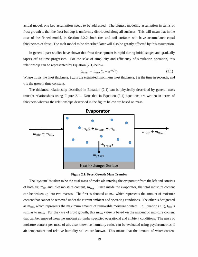
actual model, one key assumption needs to be addressed. The biggest modeling assumption in terms of

frost growth is that the frost buildup is uniformly distributed along all surfaces. This will mean that in the

case of the finned model, in Section 2.2.2, both fins and coil surfaces will have accumulated equal

thicknesses of frost. The melt model to be described later will also be greatly affected by this assumption.

In general, past studies have shown that frost development is rapid during initial stages and gradually

tapers off as time progresses. For the sake of simplicity and efficiency of simulation operation, this

relationship can be represented by Equation (2.1) below.

𝑡𝑓𝑟𝑜𝑠𝑡 = 𝑡𝑚𝑎𝑥(1 − 𝑒−𝑡/𝜏) (2.1)

Where tfrost is the frost thickness, tmax is the estimated maximum frost thickness, t is the time in seconds, and

τ is the growth time constant.

The thickness relationship described in Equation (2.1) can be physically described by general mass

transfer relationships using Figure 2.1. Note that in Equation (2.1) equations are written in terms of

thickness whereas the relationships described in the figure below are based on mass.

Figure 2.1: Frost Growth Mass Transfer

The “system” is taken to be the total mass of moist air entering the evaporator from the left and consists

of both air, mair, and inlet moisture content, mwin. Once inside the evaporator, the total moisture content

can be broken up into two masses. The first is denoted as mw, which represents the amount of moisture

content that cannot be removed under the current ambient and operating conditions. The other is designated

as mmax, which represents the maximum amount of removable moisture content. In Equation (2.1), tmax is

similar to mmax. For the case of frost growth, this mmax value is based on the amount of moisture content

that can be removed from the ambient air under specified operational and ambient conditions. The mass of

moisture content per mass of air, also known as humidity ratio, can be evaluated using psychrometrics if

air temperature and relative humidity values are known. This means that the amount of water content

20

removed across the evaporator can be estimated if evaporator air outlet temperature is also known. The

designated operational and environmental conditions will also define the mass transfer time constant, τ.

Gradually frost surface temperatures may rise to a point at which air temperature is no longer dropping

below its dew point. Frost accumulation will therefore come to a halt. This could explain the seemingly

decreasing rate of mass transfer commonly seen in application. The resulting mass transfer from the moist

air to the heat transfer surface is then taken to be mfrost, which is similar to tfrost used in Equation (2.1). The

mass leaving the evaporator can be seen to the right of Figure 2.1, consisting of the air mass content as well

as the moisture content still held by the air. This remaining moisture content will consist of mw and the

portion of mmax that did not collect on the heat exchanger surface.

One of the major benefits of simplifying the mass transfer relationship by evaluating frost thickness as

a function of time is that it allows for easy conversion into the Laplace domain and further implementation

in Simulink. Ultimately, this tool will be implemented in Simulink, so by taking advantage of Simulink’s

ability to efficiently model time dependent processes, greater simulation speed can be achieved. Figure 2.2

shows the block diagram representation of Equation (2.1). The diagram indicates that the aforementioned

mass transfer and resulting frost thickness relationships can be represented as the step response of a first

order system, with a reference step size of tmax.

Figure 2.2: Frost Growth Block Diagram

The previously discussed physical description suggests that both tmax and 1/τ are to be dependent on

operational and ambient conditions. It will therefore be assumed that both the maximum frost thickness and

growth time constant will be dependent on three parameters, those being fin pitch (FP), air velocity (V),

and temperature difference (dT) between the dew point of the moist air and the evaporator surface. This

temperature difference parameter allows for the combination of effects due to humidity, air temperature,

and surface temperature. As frost growth has been shown to be dependent on each of these parameters,

equations for maximum frost thickness and inverse of time constant will be written as a function of each

parameter and a corresponding numerically determined coefficient. Representations of each can be seen in

Equations (2.2) and (2.3). Air velocity and fin pitch will likely be constant in operation and are assumed

to be constant throughout the simulation. However, temperature difference will be allowed to change with

evaporator dynamics resulting in both tmax and 1/τ being time dependent. Though velocity and fin pitch are

21

assumed constant in the provided relationships, minute modifications can be made to Simulink models

described in later chapters to allow for these terms to also be time dependent during simulation if necessary.

𝑡𝑚𝑎𝑥(𝑡) = 𝐶1𝑉∗ 𝑉 + 𝐶1𝐹𝑃

∗ 𝐹𝑃 + 𝐶1𝑑𝑇(𝑡) ∗ 𝑑𝑇(𝑡) (2.2)

1

𝜏(𝑡) = 𝐶2𝑉

∗ 𝑉 + 𝐶2𝐹𝑃∗ 𝐹𝑃 + 𝐶2𝑑𝑇

(𝑡) ∗ 𝑑𝑇(𝑡) (2.3)

The next sub-section will further detail the means through which individual coefficients can be found.

2.1.2 Parameter Frost Growth Coefficients

Frost growth parameter coefficients are identified based on trends demonstrated by Cui et al. It should

be noted that although the coefficients discussed in this documentation are based on published modeling

data, relationships identified in other experimental and modeling studies show similar trends. This means

that the relationship presented in Equation (2.1) will hold regardless of the source. If desired, coefficients

can therefore be extrapolated individually on a case by case or system by system basis.

Cui et al. provides data points from simulated frost growth versus time for variations in fin spacing, air

velocity, relative humidity, and evaporator surface temperature. As dew point and its relationship to the

evaporator surface temperature is a major contributor to determining if and when frost growth will ensue,

these parameters have been combined into a single temperature difference value.

Using Χ2 error, maximum thickness and time constant values can be identified such that the error

between predicted frost thickness as a function of time and the data presented in the published work is

minimized for each parameter of interest. This process was completed individually for each parameter such

that when one parameter was varying, only its specific coefficient was allowed to change. All others were

kept constant during this process. Coefficients were then determined such that they are a function of their

designated parameter. Findings can be seen in the following discussion.

2.1.2.1.1 Fin Spacing

Fin pitch coefficients as a function of the fin pitch value itself can be seen in Equations (2.4) and (2.5).

Plots of these two functions can be found in Figure A.1 and Figure A.2 of Appendix A.

𝐶1𝐹𝑃= 2.8925 ∗ 10−3 ∗ 𝐹𝑃2 − 8.6917 ∗ 10−2 ∗ 𝐹𝑃 + 6.1112 ∗ 10−1 (2.4)

𝐶2𝐹𝑃= 1.3726 ∗ 10−7 ∗ 𝐹𝑃2 − 4.1753 ∗ 10−6 ∗ 𝐹𝑃 + 2.9182 ∗ 10−5 (2.5)

2.1.2.1.2 Air Velocity

For the case of air velocity, at low velocities (0.6 m/s), there was some deviation from trends seen at

higher velocities (1 m/s to 5 m/s) cases. This is believed to potentially be due to differences in behavior as

a result of laminar versus turbulent flow. As a result, the coefficients have been established as the piecewise

22

functions seen in Equations (2.8) and (2.9). Plots of these functions can be found in Figure A.3 and Figure

A.4.

𝐶1𝑉= {

−8.5495 ∗ 𝑉 + 8.552 0.6 ≤ 𝑉 < 1 −0.0349 ∗ 𝑉2 + 0.0817 ∗ 𝑉 − 0.0444 1 ≤ 𝑉 ≤ 5

(2.6)

𝐶2𝑉= {

−5.179 ∗ 10−5 ∗ 𝑉 + 5.2174 ∗ 10−5 0.6 ≤ 𝑉 < 1 9.59 ∗ 10−6 ∗ 𝑉2 − 7.86 ∗ 10−5 ∗ 𝑉 + 6.94 ∗ 10−5

𝑉21 ≤ 𝑉 ≤ 5

(2.7)

2.1.2.1.3 Dew Point to Surface Temperature Difference

Similar to the previous two cases, coefficient relationships for temperature difference were also

evaluated.

𝐶1𝑑𝑇= −1.42 ∗ 10−5 ∗ 𝑑𝑇3 + 0.00184 ∗ 𝑑𝑇2 − 0.0815 ∗ 𝑑𝑇 + 1.3644 28.43 ≤ 𝑑𝑇 ≤ 48.43 (2.8)

𝐶2𝑑𝑇= −2.0445 ∗ 10−9 ∗ 𝑑𝑇2 + 1.9135 ∗ 10−7 ∗ 𝑑𝑇 − 2.1962 ∗ 10−6 28.43 ≤ 𝑑𝑇 ≤ 48.43 (2.9)

Relationships described in Equations (2.8) and (2.9) are displayed in Figure A.5 and Figure A.6.

It is important to acknowledge that the relationships represented by Equations (2.4)-(2.9) are only valid

for a set range of parameter values. The modeling study conducted by Cui et al. provides estimation data

for only a set of test cases, which are summarized in Table 2.1.

Table 2.1: Coefficient Estimation Validity Range

Parameter Value Range

Fin Pitch [mm] 7 ≤ 𝐹𝑃 ≤ 12

Air Velocity [m/s] 0.6 ≤ 𝑉 ≤ 5

Dew Point to Surface Temperature Difference [C] 28.43 ≤ 𝑑𝑇 ≤ 48.43

The aforementioned estimations are also based upon geometry and materials specific to a particular heat

exchanger for which specifications can be seen in Table 2.2.

Table 2.2: Coefficient Estimation Heat Exchanger Specifications

Tube Outer

Diameter [mm]

Tube Thickness

[mm]

Fin Thickness

[mm]

Tube Pitch

[mm]

Tube

Material

Fin

Material

12.7 2.5 1.6 25.4 Copper Aluminum

Frost growth results associated with the above coefficient correlations will be discussed in the next section.

2.1.3 Simulation Results and Conclusions

In this section, results of a study conducted as a means of identifying trends associated with variations

in parameters such as fin pitch, air velocity, and dew point to evaporator temperature difference will be

presented. These findings will be based on the coefficient relationships extrapolated from published

modeling data using methods described in the previous section. A few cases will be analyzed for each

parameter, while keeping in mind that all of the test cases lie within the acceptable ranges described in

Table 2.1. For the study, only the parameter of interest was allowed to vary, while all others remained

23

constant. Although the following will provide a brief overview of general trends resulting from determined

coefficient correlations, Chapter 3 will provide direct comparison between findings associated with

developed correlations and those published by Cui.

2.1.3.1 Fin Spacing

In terms of fin spacing, three different fin pitches were considered, those being 8 mm, 10 mm, and

12mm. Air velocity was held constant at 1 m/s and temperature difference held at a constant value of

28.43°C. This temperature correlates to an evaporator wall temperature of -20°C and relative humidity of

90, as used by Cui et al. Figure 2.3 indicates resulting trends for frost thickness as a function of time for

varying evaporator fin spacing. Trends show that with increased fin spacing, the amount of frost growth

after a given period of time is actually lower.

Figure 2.3: Frost Thickness vs. Time for Varying Fin Spacing

Although experimental findings by Lee et al. show the opposite trend, predictions provided by Cui et

al. for overall heat transfer coefficient and pressure drop do correlate well with other studies, such as those

conducted by Yan et al. Agreement in trends associated with these parameters suggests that there may be

some validity to frost thickness findings, as both heat transfer coefficient and pressure drop are dependent

on this. As discussed in Chapter 1, there has been acknowledgement in various studies that there is

occasionally some disagreement in findings. Some of these variances could come as a result of differing

heat exchangers being used for data collection. It is therefore suggested that the coefficient extrapolation

demonstrated here be conducted on a case by case basis if more accurate results are desired.

One of the major challenges to this thesis is that without the means to conduct experiments, actual data

was difficult to come by. However, it is important to acknowledge that the demonstrated extrapolation

methods will be applicable regardless of the data source. More accurate frost growth estimations for a

specific heat exchanger are therefore likely achievable provided that experimental data is available.

24

2.1.3.2 Air Velocity

Air velocities of 0.5 m/s, 1 m/s, 1.5 m/s, and 2 m/s have been used for evaluation. A fin spacing of 10

mm and temperature difference of 28.43°C were used throughout each test. Figure 2.4 displays the

relationship between frost thickness and time for varying values of air flow velocity. Frost thickness

displays a decrease with increased air velocity. Cui proposes that is this is due to more rapid accumulation

with increased air flow. As more air is allowed to flow across the cool surface, so too is a greater amount

of moisture. This results in a thinner, denser layer of frost. These findings are additionally consistent with

experimental findings of Yan et al.

Figure 2.4: Frost Thickness vs. Time for Varying Air Velocity

2.1.3.3 Dew Point to Surface Temperature Difference

Four different case studies were conducted for determining the effect of dew point to surface

temperature difference on the rate of frost growth. Temperature differences considered were 30°C, 35°C,

40°C, and 45°C, while fin pitch and air velocity were held at 10 mm and 1 m/s, respectively.

Figure 2.5: Frost Thickness vs. Time for Varying Dew Point to Surface Temperature Difference

25

Figure 2.5 displays the results for frost thickness as a function of time for various temperature

differences. In general, the results indicate that there is a greater amount of frost accumulation after a given

period of time with increased temperature difference. This makes sense physically in that as air temperature

drops, its capacity to hold moisture similarly decreases. As the air becomes saturated, condensation will

begin to form on the cool evaporator surface. This will ultimately result in frost build up if surface

conditions are below the freezing point of water. Based on Figure 2.5, it also appears that frost thicknesses

in all cases are relatively close after 6 hours of operation. Overall, thickness differed by about a millimeter

for a total temperature difference of 15˚C.

Although the aforementioned results do reiterate typical trends seen in other past studies, predictions

are limited to hold true only within the ranges specified in Table 2.1 and for heat exchanger specifications

seen in Table 2.2. These prediction bounds are due to the limited amount of information presented in Cui

et al. Extrapolated coefficient equations are also only at most second order polynomials, so it is possible

that a higher order polynomial representation may have provided better accuracy. Additionally, data

provided in Cui et al. is modeled data, as experimental data was not available. Although these trends do

reflect common findings in other works, it is likely best to evaluate these coefficients on an actual physical

system by system basis. The relationships established in this section therefore provide a good starting point

and initial estimate for frost growth. If greater accuracy is desired, a wider range of parameter values should

be considered in addition to the use of data for a specified system. Although specific trends are in

disagreement in some cases, one thing that is agreed upon is the general relationship between frost thickness

and time represented by Equation (2.1). It is therefore important to recognize that the relationship upon

which these correlations are based will still hold true regardless of the data source.

2.2 Frost Melt

Unlike the case of frost growth, frost melt is a much more transient process occurring over timeframes

on the order of minutes rather than hours. In order to gain a better understanding of frost melt behavior and

to develop an appropriate model, it is important to be able to capture these dynamics in modeling. The

following few sections will detail the development of a frost melt model. Discussion will begin with a very

simple case involving purely cylindrical tubing to be followed by the integration of fins into the model.

Additional improvements made in the interest of greater simulation efficiency will also be addressed.

2.2.1 Preliminary Model

In order to first develop a basic understanding of the frost melt process, a very simplified model was

developed. This preliminary model made use of purely cylindrical heat exchanger tubing to eliminate

potential complications associated with fins (e.g. 2-dimensional). Through this model, general trends for

26

three key variables (temperature, enthalpy, and phase) were tracked and conclusions drawn. Evaluation of

this model allows for a basic understanding of what trends and behaviors will be expected moving forward

with a more complicated, finned model (see Section 2.2.2).

2.2.1.1 Modeling Approach

In order to establish the initial model, a few assumptions had to be introduced. One of the most

important assumptions is that there is initially uniform frost growth. Additionally, it is assumed that the

melt process is radially uniform as a result of this uniform growth. This means that at any distance, r, from

the central axis, all properties will be equivalent. Frost density and heat capacity will be estimated based

on the assumption of a 50/50 makeup of air and liquid water. The proposed density value is comparable to

values discussed in Iragorry et al. Thermal conductivity will be based on past findings by Tao et al., as

cited by Hoffenbecker, in which thermal conductivity is a function of frost density. A table of property

values used for liquid water, frost, and coil material can be found in Table C.1 of Appendix C. Although

these values were used for initial trend studies, later sections will demonstrate implementation of the model

in Thermosys™ and the ability for these parameters to be set by the user. Frost is considered to be a very

porous material, which has resulted in some studies looking further into the mass transfer occurring during

the melt process. For the sake of this study however it will be assumed that once a layer of frost has melted,

the entirety of the volume is in liquid phase. This allows for the original volume structure to be maintained

throughout the simulation. In the interest of creating an efficient model, these simplifications allowed for

a one-dimensional analysis and corresponding reduction in both computational power and time necessary.

Figure 2.6: Frost Volumetric Grid System

27

For this initial model, a finite volume method was used to simulate defrosting behavior on a tube.

Figure 2.6 displays a visualization of the cylindrical tubing model. It can be seen that there is a uniform

amount of frost growth that has occurred around the tubing. This frost is then broken up into a user-defined

number of volumes, N. In general, this choice will be based on a balance of computational time required

and accuracy. A greater number of volumes will likely correspond to a more accurate model. However,

this will also require that more equations be evaluated in addition to a potentially smaller timestep.

Requirements associated with the chosen timestep will be addressed in slightly more detail later.

Inside each of the volumes resulting from this division lies a centrally located point, or node, indicated

in Figure 2.6. As growth is initially considered uniform, the properties at any point along this radial distance

will be equivalent. These loci are represented in white. Properties evaluated at these radial distances are

average values for each of the individually designated volumes. Each volume will therefore have its own

distinct makeup and properties. These properties will be evaluated at each timestep based upon energy

equations developed in the next subsection.

2.2.1.2 Energy Equations

The first step in establishing a thermal model is to define the equations that will govern behavior. A

diagram of an energy balance for a volume being analyzed can be seen in Figure 2.7 below.

Figure 2.7: Preliminary Model Volumetric Energy Balance

The energy balance for the volume depicted above can be written such that the energy into the volume is

equivalent to the amount of energy stored plus the amount of energy leaving the system. The equation

representation of this behavior is shown in Equation (2.10).

r r r

dT dT dTcV kA kA

dt dr dr

(2.10)

28

As phase change is a constant temperature process, enthalpy was a more appropriate property to evaluate

in order to be able to track phase throughout the melt process. In terms of enthalpy, Equation (2.10) then

becomes:

r r r

dh dT dTV kA kA

dt dr dr

(2.11)

Rearranging slightly, Equation (2.12) is obtained.

1

r r r

dh dT dTkA kA

dt V dr dr

(2.12)

Using a fixed grid analysis, equations are written such that energy comes in across an inner surface and

leaves the volume across the surface at an outer radius. Heat transfer occurring at the outer radius is denoted

with an “r+Δr” subscript, while that across the inner surface is denoted with an “r” subscript. Both outer

radius surface area, Ar+Δr, and at the inner radius surface area, Ar, for the current volume of interest, Vi,

(Equation (2.15)) are represented in Equations (2.13) and (2.14).

2

2r r i

rA L r

(2.13)

2

2r i

rA L r

(2.14)

2i iV rL r (2.15)

The radius at node i is denoted ri, and is represented by Equation (2.16), where rcoil is the radius of the

evaporator coil.

(2 1)

2i coil

rr r i

(2.16)

Here, i ranges from 1 to N, where N is the number of volumes. For the defrost process, there are 7 total

phase combinations that may occur. These 7 phase sequence possibilities can be seen in Table 2.3, with F

representing frost (solid phase), T is transition phase (melting), and L is water (liquid phase). Characteristic

of phase change, only a single transition phase can be present in any three sequential nodes due to

temperature remaining constant at melting temperature throughout the process. This melting behavior then

gradually propagates through each node.

Table 2.3: Nodal Phase Combinations

1 2 3 4 5 6 7

F F F F F T L

F F F T L L L

F T L L L L L

29

The Crank-Nicolson scheme described in [30] was used for analysis due to its characteristic stability

and higher order of accuracy in comparison to both explicit and implicit solving schemes. The Crank-

Nicolson scheme is an average of both implicit and explicit schemes, providing a central differencing

approach. Central differencing often provides greater accuracy, but also comes at the price of lesser

computational speed as equations are somewhat more complex. For a central differencing approach,

differential equations can be represented as in Equations (2.17)-(2.19).

1n n

i ih hdh

dt t

(2.17)

1 1

1 10.5n n n n

i i i i

r

T T T TdT

dr r r

(2.18)

1 1

1 10.5n n n n

i i i i

r r

T T T TdT

dr r r

(2.19)

In the above equations, the timestep is indicated in the superscript, and node location as a subscript. These

designations are detailed in Table 2.4 below.

Table 2.4: Crank-Nicolson Notation

Time Iteration n Current time iteration for which enthalpy values are known

n+1 Next time iteration for which enthalpy values are being evaluated

Node Location

i+1 Next node location

i Current node of interest for which values are being evaluated

i-1 Previous node location

Energy balances can be written as a combination of the amount of energy into the volume (i.e. the

interaction between the previous node, i-1, and current node, i), as well as the amount of energy out of the

system (i.e. the interaction between the next node, i+1, and the current node, i). Using finite differencing

equations above, Equation (2.12) then becomes:

1 1 1 11 1 1 1 1

2 2 2

n n n n n n n nn n i i i i i i i ii i i r r i r

i i

T T T T T T T Tt r rh h r k r k

r r r r r r

(2.20)

For simplicity, a constant term, λ, can be pulled out, such that Equation (2.20) becomes:

1 1 1 1 1

1 1 1 12 2

n n n n n n n n n n

i i i r r i i i i i r i i i i

i i

r rh h r k T T T T r k T T T T

r

(2.21)

where

22( )

t

r

(2.22)

As the equations being solved are in terms of enthalpy, a relationship between node temperature and

enthalpy must be established for insertion into Equation (2.21). For cases in which temperature is below

that of the melt temperature, Tm, enthalpy will be considered negative. Phase transition will be present

30

when the enthalpy of the volume is between 0 and the latent heat of fusion, 334 kJ/kg. Once above this

latent heat of fusion, the volume will be in liquid state. Equation (2.23) summarizes this relationship

between temperature and enthalpy as described by Fasl [10].

im

f

i m

i latm

l

hT

c

T T

h hT

c

0

0 lat

lat

h

h h

h h

(2.23)

With this relationship, Equation (2.21) can be rewritten at each iteration based on the determined phase

of elemental volume. As previously discussed, one benefit of solving for enthalpy is that phase tracking is

easier. For the case of phase change between liquid and gas common in thermodynamics analysis the phase,

or quality (Xi), is represented by a value between 0 and 1. A similar approach can be used for phase change

from solid to liquid. In Equation (2.24), a value of 0 will be indicative of solid phase, where a value of 1

will indicate a fully melted volume, or liquid phase, similar to the approach used by Fasl [10].

0

1

ii

lat

hX

h

0

0 lat

lat

h

h h

h h

(2.24)

Ultimately, the set of N equations representing all nodal relationships for the total volume of frost can

be written into matrix form for simultaneous solving. Matrix equations take the form Ax=b. Here, the “A”

matrix is a set of coefficients associated with thermal properties at each node (Equation (2.25). The “x”

matrix represents the enthalpy values at the next time iteration, which are being solved for. Lastly, the “b”

matrix is a sum of the currently known enthalpy values at time n and any additional constants.

Aforementioned equations are written in terms of three sequential nodes (i-1, i, and i+1), resulting in the

coefficient matrix, “A”, being a tridiagonal matrix as in Equation (2.25).

0 0 0

0

0 0

0

0 0 0

y z

w y z

A

w y z

w y

(2.25)

Here, “w” coefficients are those belonging to the previous node (i-1). Designated “y” coefficients belong

to the current node for which values are being solved (i). Coefficients denoted by a “z” belong to the next

node (i+1). Note that the first and last rows in the “A” matrix only have two coefficients. This is due to

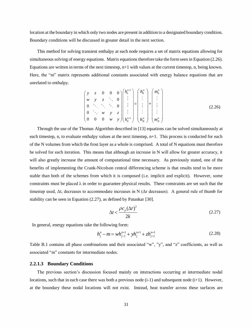
31

location at the boundary in which only two nodes are present in addition to a designated boundary condition.

Boundary conditions will be discussed in greater detail in the next section.

This method for solving transient enthalpy at each node requires a set of matrix equations allowing for

simultaneous solving of energy equations. Matrix equations therefore take the form seen in Equation (2.26).

Equations are written in terms of the next timestep, n+1 with values at the current timestep, n, being known.

Here, the “m” matrix represents additional constants associated with energy balance equations that are

unrelated to enthalpy.

0 0 0

0

0 0

0

0 0 0

y z

w y z

w y z

w y

1

0

1

n

n

N

h

h

=

0

n

n

N

h

h

+

0

n

n

N

m

m

(2.26)

Through the use of the Thomas Algorithm described in [13] equations can be solved simultaneously at

each timestep, n, to evaluate enthalpy values at the next timestep, n+1. This process is conducted for each

of the N volumes from which the frost layer as a whole is comprised. A total of N equations must therefore

be solved for each iteration. This means that although an increase in N will allow for greater accuracy, it

will also greatly increase the amount of computational time necessary. As previously stated, one of the

benefits of implementing the Crank-Nicolson central differencing scheme is that results tend to be more

stable than both of the schemes from which it is composed (i.e. implicit and explicit). However, some

constraints must be placed λ in order to guarantee physical results. These constraints are set such that the

timestep used, Δt, decreases to accommodate increases in N (Δr decreases). A general rule of thumb for

stability can be seen in Equation (2.27), as defined by Patankar [30].

2( )

2

pc rt

k

(2.27)

In general, energy equations take the following form:

1 1 1

1 1

n n n n

j j j jh m wh yh zh

(2.28)

Table B.1 contains all phase combinations and their associated “w”, ”y”, and “z” coefficients, as well as

associated “m” constants for intermediate nodes.

2.2.1.3 Boundary Conditions

The previous section’s discussion focused mainly on interactions occurring at intermediate nodal

locations, such that in each case there was both a previous node (i-1) and subsequent node (i+1). However,

at the boundary these nodal locations will not exist. Instead, heat transfer across these surfaces are

32

commonly established by means of either a constant boundary temperature or constant heat flux across the

boundary. These constant values will fall into the matrix of constants, “m” in most cases. The following

will detail the case in which a constant boundary temperature is used on both air and coil side surfaces as

well as some brief discussion of the constant heat flux case.

For cases in which a constant temperature boundary condition is present at the innermost frost radius

(coil contacting surface), an imaginary i-1 node can be implemented such that the temperature of this node

is equivalent to the boundary condition temperature. Assuming that the first existing node is 1, this new

imaginary node will have a subscript 0. Here, Tcoil is the coil surface temperature.

0 coilT T (2.29)

Combining Equations (2.21) and (2.29), the following relationship can be formed for the energy balance

equation at the interface between frost and tubing.

1 1 1 1 1

1 1 2 1 2 1 1 0 1 0

1 1

( )n n n n n n n n n n

coil r r coil rh h r r k T T T T r k T T T Tr

(2.30)

Substituting the tube wall temperature in for T0,

1 1 1 1 1

1 1 2 1 2 1 1 1

1 1

( )n n n n n n n n n n

coil r r coil r coil coilh h r r k T T T T r k T T T Tr

(2.31)

As with the case for intermediate nodes, enthalpy values will be inserted in place of temperature into

Equation (2.31) for volumes 1 and 2. This will be dependent on the determined phase of each as defined

by Equation (2.23).

A similar analysis can be conducted for the interface between the ambient air and frost. In this case,

an imaginary nodal location will be created in order to represent the imaginary i+1 node at the boundary.

This node will be called N+1. The temperature of this node will be represented by the air temperature,

Tair.

1N airT T (2.32)

Again, combining Equations (2.21) and (2.32), the resulting relationship can be established for energy

transferred at the air-frost interface, where R is the outermost radius of frost. Unlike previous cases in

which thermal conductivity was the sole contributor to thermal resistance between layers, convection must

also be taken into account here. Notice that in the first term, the radius associated with this term will be R

due to its location at the boundary.

1 1 1 1 1

1 12

n n n n n n n n n nc r rN N air N air N r N N N N

N c N r r

h k R rh h R T T T T R k T T T T

R h r k

(2.33)

Enthalpy is again evaluated at the designated nodal temperatures in accordance with Equation (2.23).

33

Energy balance equations can be rewritten as in Equation (2.34) if the amount of heat flux at the

innermost boundary is instead known, where q is the heat flux in W/m2.

1 1 1

1 1 1 1

1 1

( )n n n n n n

t t r t th h r r q r rk T T T Tr

(2.34)

Tables detailing the coefficients and constants associated with various phase combinations for constant

boundary temperature on both coil-side (Table B.2) and air-side (Table B.3) can be found in Appendix B.

Although not documented, cases in which a constant heat flux is present can be similarly represented.

2.2.1.4 Simulation Results and Conclusions

MATLAB code was written to allow for simultaneous solving of the previously discussed energy

balance equations as a means of simulating the frost melt process. Figure 2.8 contains plots of enthalpy

and phase versus time for a frost layer broken up into 5 elements. It can be seen that enthalpy of the first

volumetric node melts almost instantaneously, while the second volume gradually increases until it reaches

the enthalpy of fusion. At this point, the next volumetric node will begin the melt process. Gradually, this

behavior propagates through the entire frost layer one volume at a time. Similar behavior can be seen in

the phase plot such that when one volume completes the melt process (reaches a value of 1), the next will

follow. This is due to the fact that phase change is a constant temperature process and requires that only a

single volume be in phase change at any point in time. For phase, a value of 0 is indicative of a layer made

up entirely of frost (solid phase), while a value of 1 signifies a completely melted layer (liquid phase). The

makeup of any volume in the frost layer can therefore be determined at any point in time.

Figure 2.8: Phase (left) and Enthalpy (right) vs. Time

These findings align well with findings indicated by Fasl, in which the melt process has a propagating effect

from node to node.

34

A study was conducted in order to determine the effect the number of nodal elements has on results.

Findings can be found in Table 2.5. For the study, a frost thickness of 3mm was broken up into N volumes,

where N was allowed to range between two and ten. For each of these cases, the simulation was run for a

total of 500 seconds in simulation time. The actual time to run the simulation is also documented. In order

to meet stability requirements as discussed earlier, the timestep used for solving had to decrease with the

increase in number of volumes. The value used can be seen in the far right column of the table. It should

however be noted that these chosen timesteps do not always meet the criteria for stability, but based upon

visual results proved to provide seemingly stable results. This was done because in many cases, the timestep

actually required for this criteria was so small that even for a simulation of two volumes, the real time

required was significant. The stability requirement for two volumes called for a timestep of 0.0008 sec,

which required 2426.288 sec in real time to run the simulation. This is over four times greater than the time

being simulated. The predicted time to defrost was also equivalent to that seen in the table, suggesting that

there was no benefit to using a smaller timestep in this case.

Table 2.5: Nodal Element Study

Number

of

Elements

Time to

Defrost

[s]

Time

Change

[s]

Percent

Time

Change

Real Time

[s]

Simulation

Time [s]

Ratio of

Time

Timestep

[s]

2 106.9 13.886 500 0.027772 0.01

3 159.25 52.35 48.97100094 21.029 500 0.042058 0.01

4 187.63 28.38 17.82103611 30.517 500 0.061034 0.01

5 204.96 17.33 9.236262858 38.321 500 0.076642 0.01

6 215.91 10.95 5.342505855 47.077 500 0.094154 0.01

7 224.015 8.105 3.753878931 86.715 500 0.17343 0.008

8 230 5.985 2.671696092 250.201 500 0.500402 0.005

9 234.54 4.54 1.973913043 756.677 500 1.513354 0.003

10 241.013 6.473 2.759870385 6952.147 500 13.904294 0.001

Findings indicate that as the number of elements increases, so too does the amount of time necessary

to run the full 500 sec simulation. This is because for each time iteration, the simulation has to compute N

values, where N is the number of nodal elements. It can also be seen that the estimation for time to defrost

also gradually increases as the number of elements increases. The rate of increase is seemingly decreasing,

displaying characteristics of convergence. Figure 2.9 indicates that defrost time may still be rising,

suggesting that further convergence could be achieved by increasing the number of elements. As Table 2.5

results indicate, the time to simulate the 500 sec time frame was already about 13.9 greater with 10 volumes.

Therefore, the model may not be as useful in application if a greater number of elements were to be used

due to the extensive time requirement.

35

Figure 2.9: Predicted Time to Defrost vs. Number of Elements

Figure 2.10: Percent Prediction Time Change vs. Number of Elements

The amount of time predicted by the simulation for the frost layer to fully melt versus the number of

elements can be seen in Figure 2.9. The predicted time to defrost changes by about 134 sec, which suggest

that there could be a fairly significant amount of error in the time to defrost estimation for a low number of

elements. This effect can also be seen in the percent change in predicted defrost time (Figure 2.10). As the

number of elements increases, the predicted time gets closer and closer to the final predicted value for ten

volumes. A large number of elements also requires that the timestep be reduced, thus increasing the amount

of real time necessary to run the simulation. This can be seen in the “Real Time” column, which exhibits

an exponential increase. Ultimately, this will call for some amount of compromise between computational

time and accuracy.

The methods discussed in the above sections for representing frost melt on a cylindrical surface are

valid and do produce trends that would be expected in application. This is supported through comparison

to past works that have made use of similar methods for heat transfer and phase change ([10], [13], [30])

36

One of the biggest challenges encountered is the amount of computational time required to run a full

simulation. As the number of elements is increased, the stability of the finite differencing approach requires

that the incremental timestep used must consequently decrease. This means that some amount of tradeoff

is needed to ensure that accuracy standards are met such that determined melt time is appropriate, but also

that computational time does not become so great as to be prohibitive.

In the development of a tool aimed at predicting frost behavior accuracy, in addition to computational

time and power must be held in high regard. It would be beneficial to have a tool capable of predicting

behavior faster than it is occurring on a physical system, allowing for further use of such a tool in potentially

implementing real-time system controls. A tool such as this may become unnecessary if it is going to

require less time to simply run experiments. The simulation data presented in Section 2.2.1.4 represents

the case for only a single evaporator wall temperature. Further application in Thermosys™ may call for a

number of sections, or wall temperatures, along the evaporator surface to be analyzed. Such

implementation of the aforementioned methods would result in a much more complex and time consuming

computational problem.

As a result of some of the aforementioned drawbacks, the approach taken in creation of the finned

model will make use of different methods in an effort to improve computational efficiency and will be

detailed in further sections. It is important to note that although the methods utilized in this section will not

be carried out further, many of the trends and relationships produced as well as knowledge gained will still

be of great use moving forward and in the sections to come.

2.2.2 Finned Model

Surface area is a critical component of the heat transfer process and is therefore similarly important to

recognize the role it plays in the defrost process as well. The previously discussed “Preliminary Model”

consisted of purely cylindrical tubing as a means of gaining an initial understanding of the melt process and

some of its characteristic behaviors on a very low complexity level. This section will build off of previously

developed relationships to implement effects associated with the addition of fins.

2.2.2.1 Modeling Approach

It is first important to establish the assumptions upon which the following model is dependent. It will

again be assumed that the frost accumulation will be uniform along all surfaces, which includes both coil

and fin surfaces. Frost properties such as thermal conductivity, heat capacity, and density are assumed

constant and uniform. Although common for frost to slide off of heat transfer surfaces, gravitational effects

will be neglected such that frost will sit on the heat exchanger surface for the duration of the melt process.

37

Lastly, the heat exchanger geometry used for evaluation will be an annular finned heat exchanger (Figure

2.11).

A new modeling approach was taken in an attempt to allow for more efficient simulation of system

processes due to some of the acknowledged drawbacks associated with the finite volume approach used in

development of the preliminary model (see Section 2.2.1.4). One of the underlying goals of creating a frost

growth/melt model is to allow for implementation in the currently existing Thermosys™ Simulink toolbox.

This integration enables dynamic changes in system behavior as a result of the presence of frost to be

simulated. Simulink is commonly used in controls and is thus capable of efficiently simulating time

dependent processes. It is therefore believed that computational time can be greatly improved by applying

more of a controls approach in evaluating frost melt behavior and taking advantage of Simulink’s abilities.

The remainder of this section will therefore focus on the development of a controls-based thermal

representation of the frost melt process.

2.2.2.2 Fin Efficiency

With the addition of fins as a heat transfer surface, it is also important to note that there is some amount

of temperature loss between the base (coil surface) and the fin tip since fins are extended surfaces. Similar

to the model developed in [16], fins will be assumed annular such that the “tip” lies at the center point

between coils. Mills [25] provides Equation (2.35) for fin efficiency, ηf, for an annular fin of uniform

thickness, as seen in Figure 2.11.

Figure 2.11: Annular Fin

1 1 1 1 2 1 1 1 2

2 20 1 1 2 0 1 1 22 1

2 /f

r K r I r I r K r

K r I r I r K rr r

(2.35)

Here, r1 is the coil radius and r2 is the radius associated with the tip location. Fins are used to enhance heat

transfer as a result of convection in most cases. The β term can be represented by Equation (2.36), where

hc is the heat transfer coefficient, kt is the thermal conductivity of the fin, and tfin is the fin thickness.

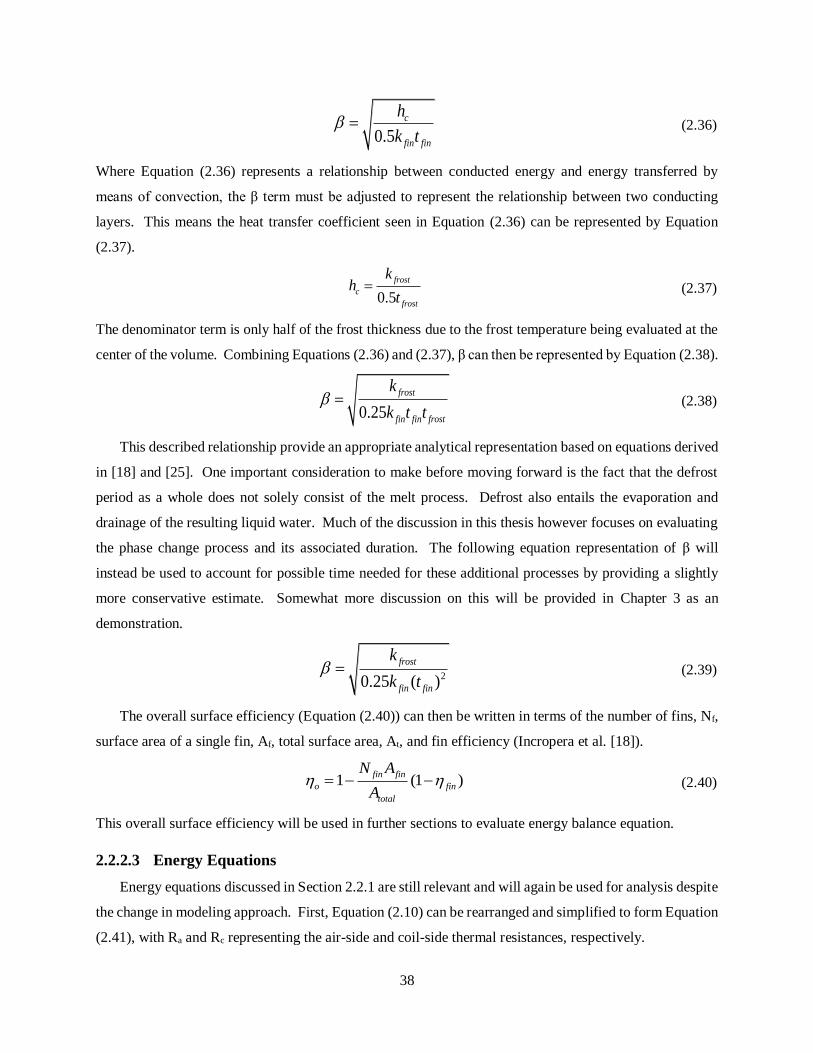
38

0.5

c

fin fin

h

k t (2.36)

Where Equation (2.36) represents a relationship between conducted energy and energy transferred by

means of convection, the β term must be adjusted to represent the relationship between two conducting

layers. This means the heat transfer coefficient seen in Equation (2.36) can be represented by Equation

(2.37).

0.5

frost

c

frost

kh

t (2.37)

The denominator term is only half of the frost thickness due to the frost temperature being evaluated at the

center of the volume. Combining Equations (2.36) and (2.37), β can then be represented by Equation (2.38).

0.25

frost

fin fin frost

k

k t t (2.38)

This described relationship provide an appropriate analytical representation based on equations derived

in [18] and [25]. One important consideration to make before moving forward is the fact that the defrost

period as a whole does not solely consist of the melt process. Defrost also entails the evaporation and

drainage of the resulting liquid water. Much of the discussion in this thesis however focuses on evaluating

the phase change process and its associated duration. The following equation representation of β will

instead be used to account for possible time needed for these additional processes by providing a slightly

more conservative estimate. Somewhat more discussion on this will be provided in Chapter 3 as an

demonstration.

20.25 ( )

frost

fin fin

k

k t (2.39)

The overall surface efficiency (Equation (2.40)) can then be written in terms of the number of fins, Nf,

surface area of a single fin, Af, total surface area, At, and fin efficiency (Incropera et al. [18]).

1 (1 )fin fin

o fin

total

N A

A (2.40)

This overall surface efficiency will be used in further sections to evaluate energy balance equation.

2.2.2.3 Energy Equations

Energy equations discussed in Section 2.2.1 are still relevant and will again be used for analysis despite

the change in modeling approach. First, Equation (2.10) can be rearranged and simplified to form Equation

(2.41), with Ra and Rc representing the air-side and coil-side thermal resistances, respectively.

39

air coil

dT dT dTcV

dt R R (2.41)

The entire volume of frost was broken up into many volumes in the finite volume approach used

previously. The modeling approach discussed in the section will instead assume that there is only a single

volume of frost representing the entire layer of frost on the heat exchanger’s surface. Additional volumes

may be added if greater accuracy is desired. It is however likely that such accuracy is not necessary,

particularly with the knowledge that additional volumes will incur some increase in computational time.

The means by which these methods are implemented also makes doing so somewhat complicated, but not

impossible. The remainder of this section will therefore assume only a single volume of frost in evaluating

energy balance equations.

Three different temperatures, Twall, Tfrost, and Tair will be used to represent temperatures of the coil, frost

layer, and air, respectively. The thermal system represented by these three components can then be

analyzed by means of thermal resistances and capacitances. A diagram of the energy flow can be seen in

Figure 2.12.

Figure 2.12: Finned Model Volumetric Energy Balance

Equation (2.42) represents the capacity of the frost layer to store thermal energy. Equation (2.43)

represents the conductive thermal resistance between the coil surface and the center of the frost layer. The

combined convective and conductive thermal resistance between the center of the frost layer and the air-

side boundary is shown in Equation (2.44).

C V (2.42)

2

frost

coil

o frost coil

tR

k A (2.43)

40

1

2

frost

air

frost air c air

tR

k A h A (2.44)

Equation (2.41) can then be rewritten with the above capacitances and resistances as Equation (2.45). The

heat capacity term, c, is absorbed into the “dT” numerator term to instead become a change in enthalpy as

a function of time. This was again done due to the benefits associated with tracking the enthalpy of the

layer rather than temperature as a result of phase change being a constant temperature process.

1 1

air frost wall frost

air coil

dhC T T T T

dt R R (2.45)

Converting to the Laplace domain for more efficient analysis in Simulink, Equation (2.46) can be obtained.

1 1

( ) (0) air frost wall frost

air coil

C H s s h T T T TR R

(2.46)

Here, h(0) represents the initial enthalpy conditions of the frost layer. Equation (2.46) can then be converted

into block diagram form. It should however be noted that Tfrost will be dependent on evaluated frost enthalpy

values and must be assessed at each timestep. Due to the complexity resulting from this dependence, a

basic representation of the governing block diagram can be seen in Figure 2.13. The “Convert to Temp”

block is used to represent the conversion from frost enthalpy, Hfrost, to frost temperature, Tfrost, in accordance

with Equation (2.23). Coil temperature, Tcoil, and air temperature, Tair, serve as reference temperatures and

appear to the left of the block diagram. The product of capacity, C, and initial frost enthalpy, h(0), can be

seen entering the system as a disturbance.

Figure 2.13: Simplified Thermal System Block Diagram

Fans are generally turned off during hot-gas defrost so natural rather than forced convection is assumed

to be occurring. Heat transfer coefficients associated with natural convection are often very low, resulting

in a lower air-side effect on the heat transfer process than that of the coil-side. This means that the impact

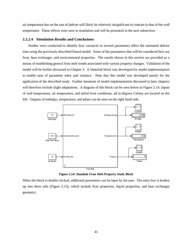
41

air temperature has on the rate of defrost will likely be relatively insignificant in contrast to that of the wall

temperature. These effects were seen in simulation and will be presented in the next subsection.

2.2.2.4 Simulation Results and Conclusions

Studies were conducted to identify how variances in several parameters affect the estimated defrost

time using the previously described finned model. Some of the parameters that will be considered here are

frost, heat exchanger, and environmental properties. The results shown in this section are provided as a

means of establishing general frost melt trends associated with various property changes. Validation of the

model will be further discussed in Chapter 3. A Simulink block was developed for model implementation

to enable ease of parameter entry and variance. Note that this model was developed purely for the

application of the described study. Further iterations of model implementation discussed in later chapters

will therefore include slight adaptations. A diagram of this block can be seen below in Figure 2.14. Inputs

of wall temperature, air temperature, and initial frost conditions, all in degrees Celsius are located on the

left. Outputs of enthalpy, temperature, and phase can be seen on the right hand side.

Figure 2.14: Simulink Frost Melt Property Study Block

When the block is double-clicked, additional parameters can be input by the user. The entry box is broken

up into three tabs (Figure 2.15), which include frost properties, liquid properties, and heat exchanger

geometry.

42

Figure 2.15: Parameter Entry Tabs

For the sake of this study, liquid properties will be kept constant at the values indicated in the “Liquid

Properties” tab in Figure 2.15 above and Table C.1 of the Appendix C. Various frost and heat exchanger

properties, as well as air and evaporator temperatures will however be allowed to vary. Only a single

parameter will be varied, while all others will remain constant for each test. A general case was first run

using the above input parameters (Figure 2.15). Results shown in Figure 2.16 serve as an initial assessment

of enthalpy, temperature, and phase behavior expected during defrost.

Figure 2.16: Enthalpy (top left), Temperature (top right), and Phase (bottom) vs. Time

43

Findings provided in Figure 2.16 reflect those presented in preliminary modeling. Enthalpy again

exhibits a gradual increase as it ultimately converges to a maximum value. This maximum value is

dependent on reference temperature conditions. Based on the temperature plot (top right), it appears that

phase change begins after about 10 seconds, at which point the temperature reaches a constant 0°C. This

temperature is maintained until the enthalpy of fusion (334 kJ/kg) is reached. Temperature will continue

to increase after the melt process has completed, gradually approaching the evaporator wall temperature.

The phase diagram (bottom) indicates the amount of the frost layer that has been melted at any point in

time. For instance, approximately half of the frost layer has been melted after about 2 min since a phase

value of about 0.5 is visible. In all, it appears that defrost requires about four minutes to complete. These

results reflect past findings, as well as what would be expected for melt behavior. The trends shown Figure

2.16 are characteristic of the melt process. Rather than provide many similar diagrams, the remainder of

this section will focus more on the effect various parameters have on the estimated defrost time.

2.2.2.4.1 Frost Properties

The first studies conducted were used to evaluate how frost property inputs affect resulting estimated

defrost time. Here, three different properties were considered, those being frost density, heat capacity, and

thickness. Note that thermal conductivity will be dependent on density, as indicated in Table C.1. The

thermal conductivity properties indicated in Table C.2 will thus be based solely on changes in density.

Frost Density

The first parameter considered is frost density. Density was allowed to vary between 300 and 450

kg/m3, while all others remained constant. Plotted results can be seen in Figure 2.17.

Figure 2.17: Time to Defrost vs. Density

Figure 2.17 displays the relationship between frost density and the predicted defrost time. Time to defrost

appears to decrease as density and thermal conductivity increase. These trends make sense in that the

44

capacity, or ability of the frost layer to store thermal energy, increases with increased density. This is

indicated by Equation (2.42). The consequential increase in thermal conductivity also allows for a faster

and more efficient spread of thermal energy throughout the layer. This greater amount of stored energy

and greater heat transfer efficiency then allows the layer to melt at a faster rate. Findings corroborate results

presented in [28] where it was determined that greater defrost efficiency was achievable with a denser

layering of frost.

Frost Heat Capacity

The next parameter considered is the heat capacity of the accumulated frost. Heat capacity was allowed

to vary between 1 kJ/kg*K and 7 kJ/kg*K. All other parameters were again kept at the values indicated in

Figure 2.14 and Figure 2.15.

Figure 2.18: Time to Defrost vs. Heat Capacity

Based on Figure 2.18, it appears that heat capacity and the estimated time to defrost have linear or

nearly linear relationship. As the heat capacity increases, so too does the time needed to eliminate the frost

layer. This could be due the absorption of the heat capacity term into the time dependent term occurring in

the transition from Equation (2.41) to Equation (2.45). An increase in enthalpy would therefore result in a

proportional increases in heat capacity, and vice versa.

Frost Thickness

The last and potentially one of the most influential parameter on the defrost process as a whole, is frost

thickness. Frost thicknesses of 1 mm, 2 mm, and 3 mm were analyzed, with findings shown in the following

diagram.

45

Figure 2.19: Time to Defrost vs. Frost Thickness

Based on Figure 2.19 above, it appears that that amount of time required to completely melt the frost layer

increases with increased frost thickness. The time to defrost increases by about 1940 sec (32 min) with an

increase of just 2 mm. Note that this time change is also highly dependent on the overall surface area. This

is because the total volume for an equivalent frost thickness will be greater with more surface area available.

This trend makes physical sense in that more energy and time will be necessary to remove a greater volume

of accumulated frost.

2.2.2.4.2 Heat Exchanger Properties

Next, heat exchanger properties were allowed to fluctuate. This again means that only a single

parameter was allowed to vary, while all other inputs remained as indicated in Figure 2.14 and Figure 2.15.

Five conditions were allowed to change, those being coil diameter, fin outer diameter, number of fins, fin

thickness, and fin thermal conductivity.

Coil Diameter

Coil diameter will be the first discussed, for which values were allowed to vary between 1 cm and 5

cm. The amount of time required for defrost as a function of coil diameter can be seen in Figure 2.20. It

appears that the amount of time needed for defrost decreases as the coil diameter increases. Since the fin

outer diameter is remaining constant while coil diameter is increased, the overall finned area begins to

decrease. Unlike fin efficiency, the coil is generally considered to be 100% efficient. This means that when

the surface area of the coil is greater (larger diameter) than that contributed by the extended surfaces, the

rate of defrost will be faster. The result of this is what is exhibited by these findings. Although not discussed

here, the reverse trend was seen when fin outer diameter was increased while maintaining coil diameter.

Time to defrost increased as fin outer diameter increased. This can similarly be explained by the discussion

above.

46

Figure 2.20: Time to Defrost vs. Coil Diameter

Fin Pitch

It is important to evaluate the effect of fin on the defrost process due to the critical role they play in the

heat transfer process and in heat exchanger design. An increased number of fins will allow for a significant

increase in surface area, providing an increase in the overall heat transfer coefficient. However, this could

also mean that a shorter refrigeration cycle will be possible if fin spacing is too small. It is likely that the

available space will be filled faster when compared to that of a relatively larger spacing with less spacing

between fins. This effect is suggested by result provided in Section 2.1.3.1.

For the study, the number of fins were varied between 400 and 800 with pass length being held constant

at 6.733 m. This allowed for effects associated with variances in fin pitch to be seen. Findings are plotted

in Figure 2.21.

Figure 2.21: Time to Defrost vs. Fin Pitch

The plot suggest that with the increase in fin pitch, the time to defrost consequently decreases. As in

the previous study, the rate at which defrost occurs consequently decreases when the fraction of total surface

47

area contributed by the fin portion of the surface increases. This is due to the efficiency of the extended

surface being much lower than that of the coil surface. The portion of overall surface area provided by the

fins increases with an increase in number of fins (decreased fin pitch), thus causing an increase in defrost

time necessary.

The growth model developed in Section 2.1 suggests that a greater amount of frost will be present

after a given period of time on a system with more closely spaced fins. Initial frost conditions would

therefore likely have been different had these systems been run in refrigeration prior to running in defrost.

For the case study presented here, it is important to acknowledge that initial frost thickness was held

constant to permit only the effect of fin pitch on the rate of defrost to be seen.

Fin Thickness

As seen in the discussion of previous sections (Equation (2.38)), fin thickness plays a major role in

determining the fin efficiency and the resulting overall surface efficiency. For this reason its effect on the

defrost process will be considered here. Tested values ranged between 0.1 mm and 0.3 mm for which

corresponding times to defrost are plotted in Figure 2.22.

Figure 2.22: Time to Defrost vs. Fin Thickness

This data indicates that the time to defrost decreases as fin thickness increases. Findings make sense

physically in that a thicker fin correlates to a greater cross-sectional area. Additional thermal energy is

therefore able to flow into the fin if heat flux is assumed constant at the coil. This will allow for a greater

amount of thermal energy to be carried to the layering of frost on the extended surface and the consequent

reduction in time to defrost. Although this seems advantageous, designers must consider that use of wider

fins will also likely require that a fewer number of fins be used. Overall surface area decreases with a lower

number of fins, reducing the effect of the evaporator and its ability to cool the environment. The associated

reduction in fin spacing with increased fin thickness could also call for more frequent defrost cycles to be

48

run since it will likely require less time to fill the existing space. This effect was not seen here since the

number of fins was held constant and cooling properties were not analyzed. However, it would likely be

the argument made by designers against increasing fin thickness despite its seemingly advantageous

properties in aiding the defrost process.

Fin Thermal Conductivity

One of the key properties associated with heat transfer and considered in selecting materials for heat

exchangers is thermal conductivity. Thermal conductivity of the fin will be the only material considered

here since the coil surface is assumed to transfer heat perfectly in calculating overall surface efficiency.

This distinction will only be necessary if fin and coil material differ. Properties for three different materials

will be considered, with those being Copper, Aluminum, and stainless steel. Materials are specified in

decreasing order of thermal conductivity values.

Figure 2.23: Time to Defrost vs. Fin Thermal Conductivity

Figure 2.23 shows that the evaporator is able to shed the accumulated frost at a faster rate when fin

material has a characteristically higher thermal conductivity. It is common for materials with high thermal

conductivity, such as Copper and Aluminum to be selected in construction of heat exchangers due to their

advanced ability to transfer heat. Simulation data corroborates this behavior since more heat is able to be

transferred with a higher thermal conductivity. The effect of this greater heat transfer is the resulting visible

decrease in required defrost time.

2.2.2.4.3 Reference Temperatures

Having thus far evaluated several of the geometric and material property effects on the melt process, it

is also important to understand what role reference temperatures of both the air and evaporator surface play

as well. For the study, evaporator surface temperature was allowed to range between 5°C and 20°C, while

air temperature will be allowed to lie between 15°C and -15°C. Note that air temperature was held at -15°C

49

while coil temperature was allowed to change. Coil temperature was similarly kept constant at 10°C when

air temperature was varied.

Coil Temperature

Results for the coil temperature case can be seen in Figure 2.24. Trends demonstrated that an increase

in coil temperature seemingly causes the time to defrost to drop dramatically. Overall behavior indicates

that coil temperature is very influential on required defrost time, with time to defrost changing by 366 sec

(about 6 min) with only a 15˚C temperature difference.

Figure 2.24: Time to Defrost vs. Coil Temperature

Air Temperature

Similar trends for air side temperature variation can be seen in Figure 2.25, in that as air-side

temperature increases, the time to defrost displays an inverse effect.

Figure 2.25: Time to Defrost vs. Air Temperature

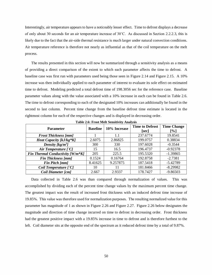
50

Interestingly, air temperature appears to have a noticeably lesser effect. Time to defrost displays a decrease

of only about 30 seconds for an air temperature increase of 30˚C. As discussed in Section 2.2.2.3, this is

likely due to the fact that the air-side thermal resistance is much larger under natural convection conditions.

Air temperature reference is therefore not nearly as influential as that of the coil temperature on the melt

process.

The results presented in this section will now be summarized through a sensitivity analysis as a means

of providing a direct comparison of the extent to which each parameter affects the time to defrost. A

baseline case was first run with parameters used being those seen in Figure 2.14 and Figure 2.15. A 10%

increase was then individually applied to each parameter of interest to evaluate its sole effect on estimated

time to defrost. Modeling predicted a total defrost time of 198.3056 sec for the reference case. Baseline

parameter values along with the value associated with a 10% increase in each can be found in Table 2.6.

The time to defrost corresponding to each of the designated 10% increases can additionally be found in the

second to last column. Percent time change from the baseline defrost time estimate is located in the

rightmost column for each of the respective changes and is displayed in decreasing order.

Table 2.6: Frost Melt Sensitivity Analysis

Parameter Baseline 10% Increase Time to Defrost

[sec]

Time Change

[%]

Frost Thickness [mm] 1 1.1 237.6774 19.8541

Heat Capacity [kJ/kg*K] 2.6075 2.86825 199.0757 0.38834

Density [kg/m3] 300 330 197.6028 -0.3544

Air Temperature [˚C] 15 16.5 196.4737 -0.92378

Fin Thermal Conductivity [W/m*K] 205 225.5 195.5320 -1.39865

Fin Thickness [mm] 0.1524 0.16764 192.8758 -2.7381

Fin Pitch [mm] 8.41625 9.257875 187.5418 -5.42789

Coil Temperature [˚C] 10 11 181.8466 -8.29982

Coil Diameter [cm] 2.667 2.9337 178.7427 -9.86503

Data collected in Table 2.6 was than compared through normalization of values. This was

accomplished by dividing each of the percent time change values by the maximum percent time change.

The greatest impact was the result of increased frost thickness with an induced defrost time increase of

19.85%. This value was therefore used for normalization purposes. The resulting normalized value for this

parameter has magnitude of 1 as shown in Figure 2.26 and Figure 2.27. Figure 2.26 below designates the

magnitude and direction of time change incurred on time to defrost in decreasing order. Frost thickness

had the greatest positive impact with a 19.85% increase in time to defrost and is therefore furthest to the

left. Coil diameter sits at the opposite end of the spectrum as it reduced defrost time by a total of 9.87%.

51

Figure 2.26: Normalized Percent Time Change Magnitude and Direction by Parameter

Figure 2.27 also displays a representation of the data presented in Table 2.6 with the exception that

only magnitude is being used for comparison. This allows for visualization of which parameters have the

greatest impact regardless of directional effect. The bar chart below is organized in descending order of

incurred time change as a consequence of the stated 10% increase.

Figure 2.27: Normalized Percent Time Change Magnitude by Parameter

Parameters ordered from left to right indicate the ranking in descending order of how sensitive predicted

defrost time is to a 10% increase in each of the parameters discussed in this section. Frost thickness exhibits

the greatest impact while density displays the least. See Figure 2.27 for a full ranking of sensitivities

associated with each of the parameters of interest.

52

Overall, the results provided in this section align well with past findings as well as what would be

expected based on a general knowledge of heat transfer. This fair alignment demonstrates the ability of the

proposed model to predict defrost time and the effect of varying input parameters on the melt process. For

these reasons, this model will be utilized in Thermosys™ implementation to be discussed in later sections.

Additional validation will be discussed in Chapter 3 of this documentation. Further details and specific

values presented in the aforementioned results can be found in Table C.2 through Table C.9 of Appendix

C.

53

Chapter 3

Model Validation

In order to demonstrate the utility of the proposed frost growth and melt models, it is first important to

validate the models proposed in previous sections. This section will therefore focus on the validation of

both frost growth and frost melt models discussed in Chapter 2. Validation will similarly be broken up into

two main sections, with those being growth and melt. Past discussion has provided some insight into the

effect various parameters have on frost behavior, but this section will provide specific examples for

comparison of results.

3.1 Frost Growth

Growth estimates will be directly compared to findings published by Cui et al. as a means of validating

the frost growth model. The particular relationship trends between frost thickness and time presented by

Cui et al. are common and likely provide a fair initial estimate of predicted frost growth after a given period

of time. Validation efforts are however not meant to prove that the effect of specific parameters on the frost

growth process are correct, as presented by Cui. Rather, they are meant to demonstrate that modeling

methods as described in Chapter 2 are applicable as long as data is available for extrapolation of

coefficients. These efforts are further meant to demonstrate that the described methods are capable of

providing good insight into the frost growth process. The discussion to follow will provide a comparison

between simulation data and published modeling data from which coefficients are deduced. The three

parameters considered (fin spacing, air velocity, and dew point to surface temperature difference) will be

individually presented in the subsections to follow.

3.1.1 Fin Spacing

Fin spacings of 7 mm, 10 mm, and 12 mm were used for comparison to published estimates. All

reference parameters therefore had to match those used by the validation reference in order to demonstrate

a direct comparison. Air velocity was resultingly kept at a value of 1 m/s and temperature difference held

at a value of 38.43˚C for all test cases.

54

Figure 3.1: Frost Thickness vs. Time by Fin Spacing Comparison

Figure 3.1 displays both the simulated results (solid lines) and published results (dashed) for frost

thickness as a function of time for varying fin spacing. Trends seem to reflect those of the available

reference data well based on the above figure. The developed model displayed an error of about 14.8% at

most.

3.1.2 Air Velocity

A similar comparison was conducted for evaluation of the model to predict variations in air velocity,

with air velocities of 0.6 m/s, 1 m/s, 3 m/s, and 5 m/s being used for comparison. Additional parameters of

interest were held constant as before. A fin pitch of 10 mm and temperature difference of 38.43˚C were

used.

Figure 3.2: Frost Thickness vs. Time by Air Velocity Comparison

Figure 3.2 above shows a comparison of predicted and published data for frost thickness as a function

of time due to changes in air velocity. Trends in this case again demonstrate fairly good alignment with

published findings. Trends in each case generally follow those provided by Cui et al., with the greatest

55

amount of visual deviation seeming to occur for the 0.6 m/s case. The greatest percent error occurs in the

3 m/s test case for which the maximum percent error is about 14.5%.

3.1.3 Dew Point to Surface Temperature Difference

Lastly, assessments of dew point to surface temperature difference predictions were analyzed. Based

upon test cases provided in available data, temperatures considered were 28.43˚C, 38.43˚C, and 48.43˚C.

A constant air velocity of 1 m/s and fin pitch of 10 mm were used in order to remain consistent with settings

used in the study being used for comparison.

Figure 3.3: Frost Thickness vs. Time by Temperature Difference Comparison

Figure 3.3 contains published trends which are indicated by a dashed line. Trends developed based on

the frost growth model proposed in this thesis are denoted by a solid line. The plot shows that there is again

decent agreement between the two with the maximum deviation from published findings being about 7.2%.

3.1.4 Conclusion

It is important to keep in mind that frost growth validation efforts here are meant more as a means of

demonstrating that the proposed model for establishing parameter coefficients used in the evaluation of

Equations (2.2) and (2.3) is valid. They are however not meant to prove the accuracy of published findings.

Published trends were used for validation in the absence of an experimental apparatus for data collection.

As noted previously, the developed model can likely provide good insight and estimates as to how much

frost will be on the evaporator after a designated period of time. Use of this model will therefore be

important moving forward in evaluating required defrost time once full cycle implementation in enabled.

It is highly recommended however that coefficients be evaluated based on experimental findings if greater

accuracy is desired. It is critical to realize that the simplified relationship defined for describing the

relationship between frost thickness and time (Equation (2.1)), as well as the method by which coefficients

56

described in this documentation have been found will remain the same regardless of the data set used. This

is why the aim of the aforementioned validation is meant to validate the method, not the actual data.

The results presented in the above sections demonstrate that reasonable results can be obtained through

the use of the frost growth modeling methods proposed in Chapter 2. For all parameters being varied (fin

pitch, air velocity, and dew point to surface temperature difference), trends matched those from which

coefficients were extrapolated, with the greatest amount of error being 14.8%. This is in contrast to the 15-

20% deviation seen by Kondepudi et al. [21]. These values were considered “good” for associated

simplified model complexity. It is however likely that these cases will in fact have the greatest agreement

as these test cases were those upon which coefficients were based. Predictions may therefore not be as

accurate for intermediate parameter values (e.g. a temperature difference of 35˚C). Results presented here

are still promising in that all of the example cases displayed good agreement between predicted and

published findings. Additionally, the model demonstrated the ability to provide fair prediction capability

over a range of values. In all, it is evident that the methods described in Chapter 2 for identifying parameter

coefficients are valid and capable of predicting trends based upon available data.

3.2 Frost Melt

Without a means to conduct experimental studies on the defrost process, published experimental data

was used for direct comparison to modeling results. Experimental data and images in this section are based

on findings discussed by Hoffenbecker [16], and will be used for evaluating previously discussed melt

model performance. This section will be broken up into three subsections. In the first, the experimental

setup used by Hoffenbecker as well as his proposed model estimations will be discussed. The second

section will detail implementation of the model proposed in this thesis and associated results. Finally, a

comparison of experimental and model simulation results will be conducted and conclusions drawn.

3.2.1 Experimentation (Hoffenbecker)

In order to validate the model proposed by Hoffenbecker, experimental studies were conducted at a

storage facility used to freeze cranberries. Operation was set on a timer-based system in which refrigeration

runs for an eight hour period. Defrost then begins with a 10 min period in which the remaining liquid phase

refrigerant left in the evaporator is able to boil off. Full defrost begins after this period, with evaporator

operation taking place at a temperature of 10˚C (50˚F) and running for a total of 45 min. This is then

followed by a 15 min cool down period after which refrigeration will resume. This cycle will continue to

repeat as is characteristic of timer-based defrost strategies.

The evaporator studied is an Imeco Model FCLS, for which specifications are detailed in Table 3.1.

Two additional parameters that are documented, but not indicated in the table below, are those of the

57

assumed fin outer diameter, which is taken to be 3.05 in (7.747 cm), and fin thickness, which is taken to be

0.01 in (0.254 mm).

Table 3.1: Imeco Evaporator Specifications [16]

Additional frost property and freezer condition information can similarly be seen in Table 3.2.

Table 3.2: Frost Properties and Freezer Conditions [16]

Experimental findings indicate that defrost of the aforementioned system required a qualitative defrost time

of about 10 to 14 min to completely eliminate the frost growth on the system (see Figure 3.6). Using the

above information, Hoffenbecker was able to predict a defrost time of 10 min and 45 seconds, which

showed good alignment with experimental findings.

3.2.2 Modeling

With a physical system for comparison as described in the previous section, the proposed model could

be put to the test for validation purposes. Minor modifications had to first be made to the block developed

for the sake of running parametric studies in Chapter 2 to allow for implementation and validation of the

frost melt model. Namely, these alterations stem from the fact that Hoffenbecker uses a blockage

percentage (see Table 3.2) rather than directly considering a frost thickness value. Equation (2.1) can then

be used to convert blockage percentage to “frost length” [16].

𝐿𝑒𝑛𝑔𝑡ℎ𝑓𝑟𝑜𝑠𝑡 = 𝑃𝑒𝑟𝑐𝑒𝑛𝑡𝑏𝑙𝑜𝑐𝑘𝑎𝑔𝑒 ∗ 𝐹𝑖𝑛𝑠𝑝𝑎𝑐𝑒 −

∆𝑖

2

(3.1)

58

Blockage percentage is therefore a gauge of the amount of the space between fins that is blocked by

frost. In this equation, Δi represents half of the fin thickness. Modification of the previous Simulink block

then allows for an amount of frost to be entered in the form of a blockage percentage. Such entry allows

for direct application of experimentally measured values. Externally, the new block will have identical

inputs and outputs to those used in Chapter 2 and can be seen in Figure 3.4. Input temperatures for the coil

surface and air are 10˚C and -15˚C, respectively. Initial frost conditions in this case will be estimated at

-28.89˚C. This initial condition was chosen based on the “Coil Temperature” value indicated in Table 3.2.

Test case trials indicate that this parameter has a small effect on prediction results. More details regarding

its associated effect will be addressed in the next section. Other options for selecting this value are to

assume either air temperature (if negative) or the average of wall and air temperature values. This is because

frost temperature will likely have a radial temperature gradient lying between air temperature and

evaporator surface temperature. Coil temperature has however been chosen for analysis because this value

correlates to the lowest possible temperature that frost could have for the specific system being considered.

The resulting time to defrost prediction will therefore be somewhat more conservative than if this initial

condition was chosen to be equivalent to the designated air temperature due to its higher value.

Figure 3.4: Hoffenbecker Validation Simulink Block

Figure 3.5 displays all of the entry tabs for the validation test case. Entries are based on frost and

evaporator specifications provided in Table 3.1 and Table 3.2. Note that rather than the frost thickness

entry tab used in the Chapter 2 parametric study (see Figure 2.15), the last entry in the leftmost image is

“Percent Blockage”. MATLAB code was used to convert this value to frost thickness using Equation (3.1).

59

Figure 3.5: Hoffenbecker Validation Parameter Entry Tabs

Although most parameters are specified in the experimental study conducted by Hoffenbecker, there

were still a few that required estimation. First, liquid properties were assumed to be those of typical water

properties. Second, frost heat capacity was assumed to be an average value of ice and air properties. Lastly,

thermal conductivity of evaporator fin material is also not designated. Since material properties indicate

that extended surfaces are aluminum (Table 3.1), fin thermal conductivity was estimated to be about 0.205

kW/m*K. The next section will detail the findings of the simulation for which parameters are described

here.

3.2.3 Results and Conclusions

Based on the aforementioned input parameters, a simulation was run to evaluate how much time is

necessary to eliminate the 23% frost blockage estimated by Hoffenbecker in experimental findings.

Enthalpy, temperature, and phase were output and used to determine the time at which defrost is complete.

Figure 3.6 displays a comparison between visuals of the experimental system, provided by Hoffenbecker

(top), and the proposed model’s simulation results (bottom). There are six total comparisons indicated in

the diagram, ranging from 0 to 14 min. Above each image is a timeframe that indicates the time range in

which the photos were taken and during which the below descriptions held true. Simulation phase versus

time results are plotted as a solid line. The shaded overlay represents the timeframe indicated above each

image as a means of providing a direct comparison of where simulation phase change lies during the

designated timeframe. For instance, the first image displays the evaporator at some point during the first

four minutes of operation in defrost. This range of time is indicated by the shaded region on the plot below.

During this timeframe, Hoffenbecker notes the “initiation of defrost with frost visibly starting to melt”.

Simulation data indicates that about 40% of the frost layer completes the melt process during this four

minute time period, with an indicated phase value of about 0.4.

60

Figure 3.6: Experimental (Hoffenbecker [16]) vs. Simulation Results

In all, the simulation predicts a total defrost time of 11 min and 4 sec, which lines up fairly well with

Hoffenbecker’s qualitative estimate of 10 to 14 min. Note that these results were obtained when the more

conservative β estimate (Equation (2.36)) was used. With the less conservative β term (Equation (2.38)),

61

defrost time was estimated at about 6 min. Based on Hoffenbecker’s visual analysis, there is “mostly water

drainage” occurring at this point during the defrost cycle. This lines up well with the fact that phase change

is complete, as was hypothesized in Chapter 2. A more conservative version of the β term is however

necessary to account for the remaining drainage and evaporation. These results demonstrate that improved

predictive capability can be achieved by using a more conservative approach and will therefore be used in

all implementation and discussion moving forward.

Run time must be designated in order to simulate the described system. As Hoffenbecker indicates that

the total time allotted for defrost in the experimental system is 45 min, the Simulink simulation time was

also set to 45 min for consistency. Full simulation of this 45 min time period required just under 2 sec to

complete using a variable step solver.

Previous discussion noted that the assumed initial frost temperature also had the potential to change the

estimated defrost period needed. When an initial condition of -22˚C (midpoint of “coil temperature” and

“freezer temperature”) was used, defrost time was estimated to be 10 min and 46 sec. This indicates that

the initial condition estimate has relatively little effect on the overall end result, as this timeframe is still

within Hoffenbecker’s qualitative analysis. Findings presented in Section 2.2 indicate that time to defrost

results are also sensitive to variations in other parameters as well and are highly subject to user input. It is

therefore possible that a lower or higher prediction time is possible since some parameters were left to be

estimated (e.g. fin thermal conductivity).

It is important to again be reminded that Hoffenbecker specifies that the evaporator being used for

analysis runs in defrost for a total of 45 min on a timer-based schedule. Both experimental findings and

simulated results however show that only a third of the total allotted defrost time was needed to fully remove

the accumulated frost. The results here suggest that energy consumption could be greatly reduced if a

greater knowledge and prediction capability of the amount of frost present on the evaporating system is

available. This example demonstrates one of the biggest drawbacks of methods commonly used in

refrigeration systems today, and just how useful the model-based prediction approach developed for this

thesis can be in helping to reducing both energy consumption and costs associated with such.

Despite the indicated sensitivity to parameter input, these results do show good prediction capability

in that they not only provide a prediction on the correct order of time, but that they are also able provide a

result that lies within the experimentally found qualitative estimate. In addition to the demonstrated

predictive capability, efficiency of the tool was also shown in that only 2 sec were required to fully run the

simulation. Future sections will therefore make use of this model for further defrost implementation in

Thermosys™.

62

Chapter 4

Thermosys™ Implementation

Besides just being able to develop the frost growth and frost melt modeling methods detailed in previous

chapters, one of the major goals of this thesis is to also allow this knowledge to be used in further predicting

resulting dynamic system behavior. Chapter 1 provides a brief background of published findings to date,

indicating the substantial amount of work that has gone toward understanding the frost growth and melt

processes in addition to operational effects common in systems running under frosting conditions. Despite

these efforts, few studies actually consider the coupled dynamic behaviors of both frost and system

operation. This is a critical aspect to consider since the behavior of each is dependent on the other.

Furthermore, to the author’s knowledge, there is not currently a tool that allows for joint dynamic behavior

of vapor compression systems and frosting behavior in both cooling and defrost modes of operation.

This chapter will detail a brief overview of the Simulink blocks developed for implementation of the

aforementioned frost growth and melt models in the Thermosys™ framework. Additional discussion will

take a look at the evaporator component currently available in Thermosys™ as well as some of the

modifications made to allow frosting effects to be seen in system operation. The last section will then cover

full vapor compression cycle execution consisting of operation in cooling and hot-gas defrost. Introduced

frost growth and melt models will then be jointly applied to full system dynamics for analysis.

4.1 Thermosys™ Overview

Thermosys™ is a commercially available MATLAB/Simulink library that was developed at the

University of Illinois as a means of allowing for the dynamic simulation of air conditioning and refrigeration

systems. The library contains various components common in vapor compression systems (e.g. evaporator,

compressor, condenser, expansion devices, etc.) and refrigerant properties. Through the use of

Thermosys™, system operating conditions (e.g. wall temperature) may be obtained and used as input

parameters for the introduced frost growth and melt models. This means that frost behavior will be allowed

to dynamically behave as changes in operation of the vapor compression system occur. Similarly, system

63

behavior will consequently be impacted as the amount of frost increases or decreases. One key benefit of

making use of a currently available and validated framework for implementation is that complications

associated with obtaining system operating conditions may be mitigated.

4.2 Frost Growth Model

Discussion on frost growth modeling has been focused on the derivation of modeling methods thus far.

This section will instead focus on actual implementation of the developed techniques. As has been

previously stated, modeling efforts have been somewhat tailored for use in Simulink due to its ability to

efficiently represent time dependent relationships. The following block (Figure 4.1) was therefore

developed for evaluating the amount of frost on an evaporator after given period of time through the use of

MATLAB code and Simulink. Code execution was based upon methods described in past chapters.

Figure 4.1: Frost Growth Simulink Block

Block inputs of wall temperature and air temperature can be seen on the left hand side of Figure 4.1.

One of the benefits of Simulink is that it allows for ease of signal rerouting through the use of a tag system.

This means that dynamic wall temperature outputs associated with evaporator behavior can be directed as

inputs to the above frost growth block when run as a full vapor compression cycle. Another example of

how signal routing is used in simulation is in regard to air temperature, which is used as an input value for

simulating both frost growth and evaporator behavior. A single air temperature signal can therefore be

routed to both components for use as an input. These values can also be designated as constants or by other

means if analysis as a standalone component is desired. An example of both standalone and full cycle

operation will be shown in the sections to follow.

Additional ambient conditions must be specified by the user to supplement the externally visible wall

temperature and air temperature inputs. Entry of these conditions may be completed by double-clicking

the Simulink block. Once open, the two entry tabs seen in Figure 4.2 and Figure 4.3 will be visible. Figure

4.2 displays the “Ambient Conditions” tab in which fin pitch, air velocity, and relative humidity must be

specified.

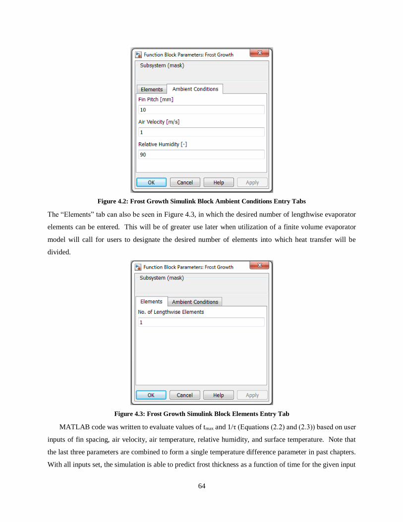
64

Figure 4.2: Frost Growth Simulink Block Ambient Conditions Entry Tabs

The “Elements” tab can also be seen in Figure 4.3, in which the desired number of lengthwise evaporator

elements can be entered. This will be of greater use later when utilization of a finite volume evaporator

model will call for users to designate the desired number of elements into which heat transfer will be

divided.

Figure 4.3: Frost Growth Simulink Block Elements Entry Tab

MATLAB code was written to evaluate values of tmax and 1/τ (Equations (2.2) and (2.3)) based on user

inputs of fin spacing, air velocity, air temperature, relative humidity, and surface temperature. Note that

the last three parameters are combined to form a single temperature difference parameter in past chapters.

With all inputs set, the simulation is able to predict frost thickness as a function of time for the given input

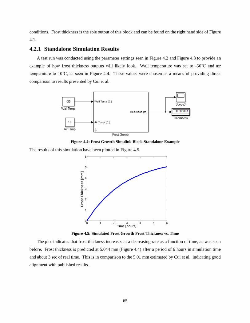
65

conditions. Frost thickness is the sole output of this block and can be found on the right hand side of Figure

4.1.

4.2.1 Standalone Simulation Results

A test run was conducted using the parameter settings seen in Figure 4.2 and Figure 4.3 to provide an

example of how frost thickness outputs will likely look. Wall temperature was set to -30˚C and air

temperature to 10˚C, as seen in Figure 4.4. These values were chosen as a means of providing direct

comparison to results presented by Cui et al.

Figure 4.4: Frost Growth Simulink Block Standalone Example

The results of this simulation have been plotted in Figure 4.5.

Figure 4.5: Simulated Frost Growth Frost Thickness vs. Time

The plot indicates that frost thickness increases at a decreasing rate as a function of time, as was seen

before. Frost thickness is predicted at 5.044 mm (Figure 4.4) after a period of 6 hours in simulation time

and about 3 sec of real time. This is in comparison to the 5.01 mm estimated by Cui et al., indicating good

alignment with published results.

0 1 2 3 4 5 60

1

2

3

4

5

6

Time [hours]

Fro

st

Th

ickn

ess [

mm

]

66

4.3 Frost Melt Model

Unlike the frost growth model discussed in Section 4.2, use of the frost melt model in Simulink has

been introduced briefly in past sections. Earlier introduction was intended to simplify execution of

parametric and validation studies discussed in previous chapters. Minor modifications have been made in

an effort to make the model more easily applicable for use with full vapor compression cycle dynamics and

more informative for potential users. This new block can be seen in Figure 4.6 below.

Figure 4.6: Frost Melt Simulink Block

Many of the external inputs (left) used in this new block are the same as those specified in the Simulink

block used for conducting the parametric study featured in Chapter 2, as well as validation efforts in Chapter

3. Those inputs being wall temperature, air temperature, and initial frost temperature conditions.

Conditions for wall temperature and air temperature inputs are identical to those used in the frost growth

model. Wall temperature is therefore based upon evaporator simulation outputs while in defrost cycle

implementation and air temperature is equivalent to the assigned evaporator air temperature input. Frost

thickness as an external input is the only visible difference from previous iterations, as it was previously

located in an entry tab. This change was made as a means of allowing initial frost thickness to be based

upon outputs of a previously run refrigeration cycle if desired.

Full cycle modeling configurations, which will be discussed in greater detail in Section 4.5, are

designed such that a cooling cycle may be run in a Simulink workspace. Final evaporator surface

temperatures and frost thickness values are then saved to the MATLAB workspace. These saved variables

can then be called from the workspace for use as inputs in a separate hot-gas defrost Simulink model.

Comparable to the frost growth block described in the previous section, this block is also applicable in a

standalone configuration for which constant input values are used. This means that results are also

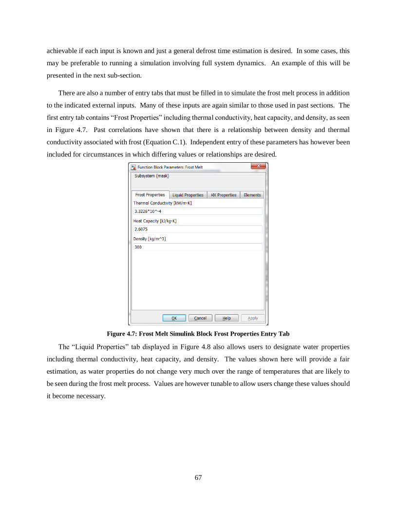
67

achievable if each input is known and just a general defrost time estimation is desired. In some cases, this

may be preferable to running a simulation involving full system dynamics. An example of this will be

presented in the next sub-section.

There are also a number of entry tabs that must be filled in to simulate the frost melt process in addition

to the indicated external inputs. Many of these inputs are again similar to those used in past sections. The

first entry tab contains “Frost Properties” including thermal conductivity, heat capacity, and density, as seen

in Figure 4.7. Past correlations have shown that there is a relationship between density and thermal

conductivity associated with frost (Equation C.1). Independent entry of these parameters has however been

included for circumstances in which differing values or relationships are desired.

Figure 4.7: Frost Melt Simulink Block Frost Properties Entry Tab

The “Liquid Properties” tab displayed in Figure 4.8 also allows users to designate water properties

including thermal conductivity, heat capacity, and density. The values shown here will provide a fair

estimation, as water properties do not change very much over the range of temperatures that are likely to

be seen during the frost melt process. Values are however tunable to allow users change these values should

it become necessary.

68

Figure 4.8: Frost Melt Simulink Block Liquid Properties Entry Tab

The fourth tab in which parameter values must be entered is the “Heat Exchanger Properties” tab.

Geometric properties including coil diameter and number of fins are to be specified here in addition to fin

thermal conductivity. The full list of required entry parameters can be seen in Figure 4.9.

Figure 4.9: Frost Melt Simulink Block Heat Exchanger Properties Entry Tab

Similar to the frost growth block discussed in the previous section, an additional “Elements” tab has

been added to allow users to designate the number of volumes into which the evaporator will be broken up.

69

Note that this will then also be the number of wall temperatures that will be used as external inputs. Again,

this will be of greater importance when evaporator dynamics are being used to evaluate frost melt behavior.

Details of this will be discussed at greater length in later sections.

Figure 4.10: Frost Melt Simulink Block Elements Entry Tab

As with the block inputs, most of the outputs (right side of Figure 4.6) remain the same as those

presented in past discussion. The sole difference here being remaining thickness. Where all other outputs

present more of a physics based information set of the melt process, remaining thickness allows for slightly

better visualization of melt progress. This insight is supplementary to the provided ability to couple frost

and system dynamics during defrost cycle simulation. Greater discussion regarding full cycle

implementation and the indicated coupled behavior will be conducted in Section 4.5.

4.3.1 Standalone Simulation Results

As a demonstration of how this block can be applied as a standalone system as well as its associated

outputs, an example simulation has been setup (Figure 4.11). All other input parameter values can be seen

in Figure 4.7 through Figure 4.10. Note that these inputs are identical to those used in the validation efforts

described in Chapter 3, with the designated 23% frost blockage being converted to 1.81 mm of frost. This

value can be seen in the lower left corner of Figure 4.11.

70

Figure 4.11: Frost Example Simulink Block Standalone Example

All four output plots of the 15 min simulated timeframe can be seen in Figure 4.12. Enthalpy is located

in the top left, temperature in the top right, phase in the bottom left corner, and remaining thickness in the

lower right. Final simulation values for each of these can be seen in the display boxes to the right side of

Figure 4.11. Time to defrost can be estimated visually through the use of any of the provided plots, though

this approximation is more easily done with some than with others.

From enthalpy, melt is estimated to be completed when the enthalpy value reaches that of the enthalpy

of fusion (334 kJ/kg). This evaluation however is slightly more difficult to do visually than any of the

remaining three. From the temperature plot, the layer has finished the melt process when temperature rises

above the constant phase change temperature of 0˚C. Based on the phase plot, time to defrost is estimated

according to when phase reaches liquid phase, which is denoted by a phase value of 1. Lastly, and perhaps

most evidently, melt time can be estimated by the frost thickness plot. Defrost is complete when this value

reaches 0 mm.

71

Figure 4.12: Simulated Frost Melt Enthalpy (top left), Temperature (top right), Phase (lower left), and Frost

Thickness (lower right) vs. Time

As indicated by each of the above plots, the time to defrost is estimated at about 11 min. Results here

are consistent with validation findings provided in Chapter 3.

4.4 Finite Volume Evaporator

Where the past two sections have focused on converting previously discussed modeling methods into

components applicable in the Simulink and Thermosys™ framework, discussion here will be geared more

toward modifications made to existing modeling components to allow for the aforementioned coupled

dynamics to also be seen in system operation. More specifically, these alterations were made to the existing

evaporator component due to it being the component most directly impacted by operation under frosting

conditions.

In past versions of Thermosys™, evaporator models have made use of lumped parameters to identify

zones of two-phase and gas phase refrigerant and their associated properties. One of the challenges with

that implementation in regard to frost dynamics is that zone lengths were allowed to change throughout the

72

simulation. Since it was a lumped parameter model, all of the two-phase region was assumed to have

uniform properties and so too was the gas phase region. It was therefore difficult to get an accurate reading

on individually sectioned wall temperatures, as are necessary for the previously described frost growth and

melt models. Further development of a finite volume model (Figure 4.13) has allowed zone lengths to be

kept constant and enabled direct tracking of wall temperatures. It should therefore be noted that

implementation of frost growth/melt models requires the use of a finite volume evaporator.

Figure 4.13: Finite Volume Evaporator Simulink Block

The figure indicates that inputs of air mass flow, air inlet temperature, refrigerant inlet and outlet mass

flow, as well as refrigerant inlet enthalpy are needed. As before, additional parameters can be entered by

double-clicking the component. There are a total of six entry tabs, those being evaporator geometry, wall

properties, parameter adjustment factors, refrigerant/air properties, initial conditions, and simulation. As

these values are of less importance, individual tabs will not be discussed here, but can be viewed in

Appendix D.

The tab that is likely of greatest significance for the discussion presented here is the simulation tab

(Figure D.6). Here, users can designate the desired number of volumes into which the evaporator will be

evaluated, with values ranging from 2-10. This value will then also be used as an input to the frost growth

and melt models, as described in the past two sections.

73

One of the drawbacks of current Thermosys™ modeling is that it does not take into consideration

possible frosting effects exhibited by systems operating under frosting conditions. This means that for

systems operating above the freezing point of water, current modeling likely provides a fair estimate of

system dynamics. However, operating conditions below the 0˚C point are not uncommon in refrigeration

applications and therefore require that the influence frost behavior on system dynamics in both cooling and

defrost be taken into account.

Having a finite volume model to build off, modifications were made to allow effects associated with

the presence of frost to be seen. The previous two sections covering the frost growth model and frost melt

model describe the need in full cycle implementation for evaporator surface temperatures to be used as

inputs. Something important to realize is that the frost growth process is causal. This means not only that

frost growth and melt are based upon evaporator behavior, but that evaporator behavior is similarly

dependent on frost behavior. As a result, frost thickness is also needed as feedback into the evaporator

component. The remainder of this section will detail methods used for determining surface efficiency due

to frost layering, as well as the application of these methods in the development of a new finite volume

evaporator Simulink block. Results for a standalone configuration will also be presented in Section 4.4.3.

4.4.1 Surface Efficiency

The presence of frost is a common plague in the refrigeration industry and is important to

correspondingly acknowledge in simulation. Existing Thermosys™ modeling methods do an adequate job

of providing insight into system operational dynamics in cases where frost is not likely to be present,

however, changes must be made to account for the associated performance degradation in instances when

that is not the case. One means of accounting for this is to treat the newly frosted surface as a composite

fin. Tu et al. provides Equations (4.1) and (4.2) for a composite fin where the coating layer has a smaller

thermal conductivity than that of the heat exchanger material. Since heat exchanger material selection is

greatly influenced by the material’s thermal properties, particularly high thermal conductivity, it is fair to

assume that the thermal conductivity of the fin will be greater than that of the frost coating.

1 1 1 1 2 1 1 1 2

2 20 1 1 2 0 1 1 22 1

2 /cos( ) sin( )

2

fin fin

f frost frost

frost

k t r K r I r I r K rt t

k K r I r I r K rr r

(4.1)

(0.5 )

c

avg fin frost

h

k t t

(4.2)

This fin efficiency representation is very similar to the frost melt model presented in Chapter 2. The

sole exception here is the addition of the bracketed terms seen in Equation (4.1). More information

regarding what r1 and r2 represent geometrically can be found in Figure 2.11. Here, kavg is a volumetric

74

average thermal conductivity of the “composite” fin. Fin efficiency described by Equation (4.1) along with

the efficiency of the frost covered tubing allows for the determination of an overall surface efficiency

(Equation (4.3)). Overall surface efficiency can therefore be written in terms of the number of fin, Nf,

surface area of a single fin, Af, total surface area, At, and fin efficiency (Incropera et al. [18]).

1 (1 )fin fin

o fin

total

N A

A (4.3)

This equation assumes that the coil wall is capable of transferring 100% of its energy to the surrounding

air. Although this is usually a fair assumption since heat exchanger surfaces are very conductive, the built

up frost layer will contribute additional thermal resistance and result in a lower coil efficiency. Equation

(4.3) can be modified slightly to reflect this, with ηcoil representing the efficiency of the coil in the presence

of frost. The new representation is shown in Equation (4.4) Note that in the circumstance in which there

is not any frost, ηcoil will just be 1.

( )fin fin

o coil coil fin

total

N A

A (4.4)

In order to evaluate this new base efficiency, the thermal conductivities due to both conduction and

convection must be determined as in Equation (4.5) and Equation (4.6), respectively.

log( / )

2

fin coil

cond

coil fin

d dR

L k (4.5)

1conv

c coil

Rh A

(4.6)

In general, efficiency is represented by the ratio of actual heat transfer to maximum heat transfer (Equation

(4.7)).

max

actualQ

Q (4.7)

For base efficiency, this will be the ratio of amount of heat transfer due to conduction through the frost

layer and associated convection to the convection heat transfer that would solely be present without the

existence of frost. In terms of resistances, this can be estimated as the ratio of thermal resistance associated

with convection to the overall thermal resistance (Equation (4.8)).

convcoil

cond conv

R

R R

(4.8)

The coil is assumed to be a perfect conductor in evaluation of the above thermal resistances.

Current Thermosys™ modeling techniques make use of the number of heat transfer units method

(NTU), with an assumed 100% surface efficiency in evaluating heat transfer dynamics. In order to then

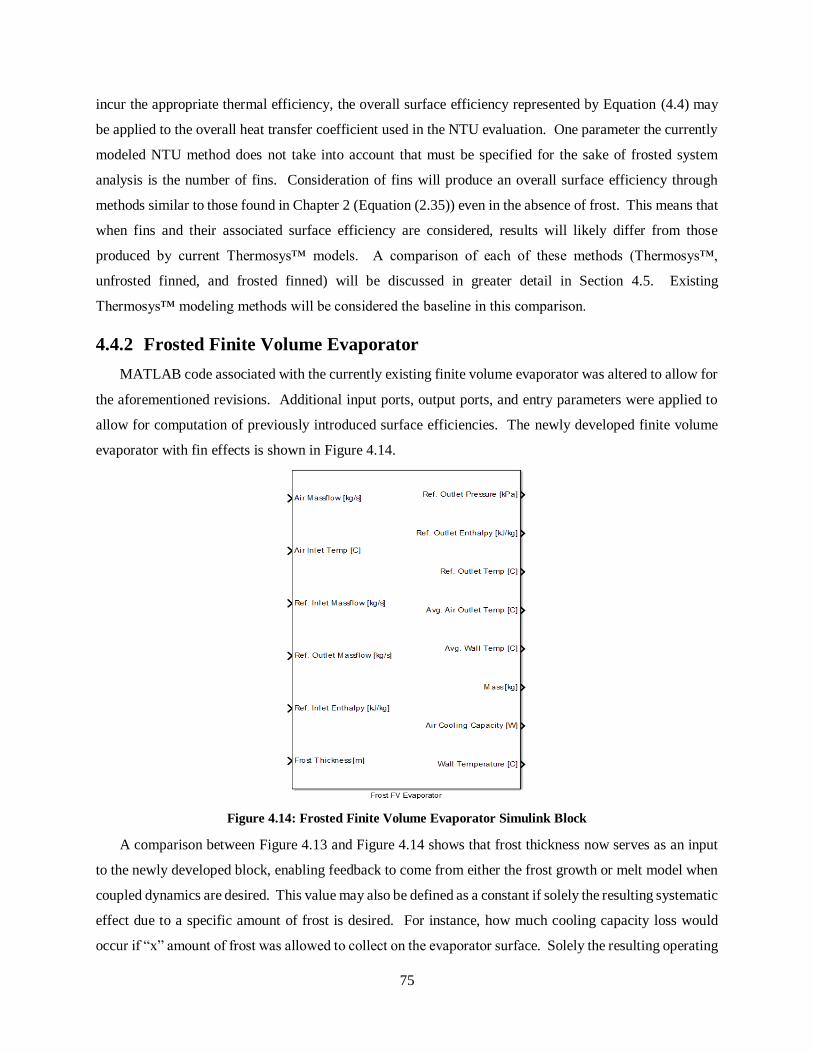
75

incur the appropriate thermal efficiency, the overall surface efficiency represented by Equation (4.4) may

be applied to the overall heat transfer coefficient used in the NTU evaluation. One parameter the currently

modeled NTU method does not take into account that must be specified for the sake of frosted system

analysis is the number of fins. Consideration of fins will produce an overall surface efficiency through

methods similar to those found in Chapter 2 (Equation (2.35)) even in the absence of frost. This means that

when fins and their associated surface efficiency are considered, results will likely differ from those

produced by current Thermosys™ models. A comparison of each of these methods (Thermosys™,

unfrosted finned, and frosted finned) will be discussed in greater detail in Section 4.5. Existing

Thermosys™ modeling methods will be considered the baseline in this comparison.

4.4.2 Frosted Finite Volume Evaporator

MATLAB code associated with the currently existing finite volume evaporator was altered to allow for

the aforementioned revisions. Additional input ports, output ports, and entry parameters were applied to

allow for computation of previously introduced surface efficiencies. The newly developed finite volume

evaporator with fin effects is shown in Figure 4.14.

Figure 4.14: Frosted Finite Volume Evaporator Simulink Block

A comparison between Figure 4.13 and Figure 4.14 shows that frost thickness now serves as an input

to the newly developed block, enabling feedback to come from either the frost growth or melt model when

coupled dynamics are desired. This value may also be defined as a constant if solely the resulting systematic

effect due to a specific amount of frost is desired. For instance, how much cooling capacity loss would

occur if “x” amount of frost was allowed to collect on the evaporator surface. Solely the resulting operating

76

conditions will be observed when frost thickness is specified as a constant because system dynamics will

converge directly to operating conditions associated with the designated amount of frost. This type of

implementation will be discussed at greater length in the next sub-section.

Output are again designated to the right of the Simulink block. Figure 4.14 indicates that a wall

temperature port has now been added. This output will display the wall temperature of each of the N

segments, where N is the number of designated evaporator volumes. The output temperature distribution

can then be used as an input to the aforementioned frost growth and frost melt models. Decisions regarding

which of these two models will be used is dependent on the mode of operation being simulated (i.e. frost

growth will be used in cooling and frost melt used during defrost). In each case, interconnectivity will

allow operational dynamics to similarly affect those associated with frost behavior.

As was stated at the beginning of this sub-section, in addition to a greater number of inputs and outputs

externally, supplementary information is also needed to evaluate the newly defined surface efficiencies. In

all, this requires that changes be made to two entry tabs, those being “Evaporator Geometry” and “Wall

Properties”. The addition of a new “Frost Properties” tab is also needed. The “Evaporator Geometry” tab

is displayed in Figure 4.15. When compared to Figure D.1, located in Appendix D, fin thickness, center to

center coil distance (i.e. fin outer diameter), and the number of fins are the three additions to this tab.

Figure 4.15: Frosted Finite Volume Evaporator Simulink Block Evaporator Geometry Entry Tab

77

The “Wall Properties” tab is shown in Figure 4.16, in which the only visible difference to this tab is an

additional entry space for wall thermal conductivity. Although not shown in this documentation due to the

addition of only a single entry, the “Frost Properties” tab allows for the entry of a frost thermal conductivity

value.

Figure 4.16: Frosted Finite Volume Evaporator Simulink Block Evaporator Geometry Entry Tab

Many of these new entry parameters are visibly identical to those already used in the developed frost

growth and frost models. Entry will therefore likely require a copy and paste. Although not completed for

this thesis, future work discussed in Chapter 5 includes the allowance of these repeated terms to be entered

only once to suitably define the model. This simplification will also enable the tool to be more

straightforward for potential users.

4.4.3 Standalone Simulation Results

The newly developed frosted finite volume evaporator will be analyzed in this section to demonstrate

that expected behaviors hold true. Solely the aforementioned frosted finite volume evaporator (Section

4.4.2) was used as a standalone component for the sake of demonstration. This means that dynamics

associated with other vapor compression system components have been neglected. Evaporator inlet signals

are generally dependent on these dynamics when in full cycle implementation is applied, however have

been held constant in their absence. Dynamics of a full vapor compression system (evaporator, compressor,

condenser, and electronic expansion valve) will be analyzed later in Section 4.5.

As the focus of this section is to demonstrate the effect of frost on the performance of the modeled

evaporator, the frost growth model was not used. Frost thickness was instead input as a constant value,

ranging from 0 mm to 4 mm. It was assumed that the designated frost growth is evenly distributed along

the entire length of the evaporator, meaning that this thickness was applied to each of the N segments into

78

which the evaporator has been broken up. A number of simulations were therefore run to show the effect

an increased frost thickness has on performance. It is important to note here that input parameters, with the

exception of frost thickness, will not be specified in as great of detail as they have in the past. This is

because the aim of this section is to evaluate the overall qualitative effect the presence of frost has on system

operation, not necessarily its effect on a particular system. The trends presented here will therefore likely

be similar from system to system. However, values specific to each system will undoubtedly differ due to

their dependence on specified operating conditions and system geometry.

In each case, simulations were run for a total of 1 hour in simulation time to allow the system to reach

steady state operation. Simulation outputs for refrigerant cooling capacity as a function of input frost

thickness can be seen in Figure 4.17.

Figure 4.17: Evaporator Cooling Capacity vs. Frost Thickness

The figure indicates that with increased frost thickness, the cooling capacity that the evaporator is able

to deliver to the environment decreases exponentially, as would be expected. With additional thermal

resistance due to the thickening frost layer, the system is not capable of providing optimal heat transfer. In

initial stages of frost growth, the additional layering has been shown to actually increase the amount of

surface area (Chapter 1), which is able to counteract thermal resistance effects to some extent. Over time,

this increased surface area is no longer able to overcome the degradation of system performance due to the

presence of frost and likely results in the above exponentially decreasing behavior.

79

Figure 4.18: Evaporator Air Outlet Temperature vs. Frost Thickness

Figure 4.18 displays the relationship between air outlet temperature and frost thickness. Consistent

with a decrease in cooling capacity, air outlet temperature increases with increased frost thickness. The

accumulated layer of frost creates an additional thermal resistance, causing the above decrease in cooling

capacity. By definition, this means that the evaporator is no longer capable of removing the same amount

of heat from the ambient air and results in the visible air outlet temperature increase.

Figure 4.19: Evaporator Refrigerant Outlet Temperature vs. Frost Thickness

Consequently, the refrigerant outlet temperature begins to decrease as the cooling capacity of the

system is no longer able to remove as much thermal energy from the environment. This effect can be seen

in Figure 4.19.

80

Figure 4.20: Refrigerant Outlet Pressure vs. Frost Thickness

Lastly, effects on evaporator outlet pressure are also presented in Figure 4.20. As frost thickness

increases, the refrigerant outlet pressure follows a similar decreasing trend as that displayed by refrigerant

outlet temperature. Experimental studies such as those conducted by Ali have shown similar trends in that

with increased frost accumulation the pressure drop across the evaporator increases. This idea is supported

by the aforementioned findings. Inlet evaporator conditions (e.g. pressure) for the study presented in this

section are maintained constant throughout simulation. Constant inlet conditions in conjunction with the

indicated outlet pressure decrease in Figure 4.20 demonstrate an overall increased pressure drop across the

heat exchanger. Actual data represented in each of these plots can be found in Table D.1 of the Appendix.

As a supplement to the results presented in this section, additional runs were conducted to see how this

effect varied based on the number of fins and resulting change in surface area. The evaporator used in this

study was defined as having 300 fins. The results for both a 500 finned and 700 finned system can also be

seen in Table D.2 and Table D.3, respectively. Similar trends for each case were found. It should be noted

that the length of the evaporator was kept constant in each of these cases. This resulted in varying fin pitch

and overall surface area. The effect of increased surface area can be deduced from the fact that maximum

capacity and the capacity associated with 4 mm of frost growth increased with an increased number of fins.

Overall, the simulated trends reflect behavior that would be expected in application and are consistent

with published findings. Chapter 1 details the use of defrost cycles as a means of eliminating the effects of

frost growth on system performance. This simulation data corroborates these negative effects and supports

the primary motivation for the implementation of defrost. Further, findings also demonstrate the utility of

methods proposed in this thesis aimed at improving the associated operational efficiency.

81

4.5 Full Vapor Compression Cycle Implementation

The previous sections in this chapter have thus far given an overview of each of the key modeling

components that will be used to simulate frost behavior and its effects on system performance. This section

will be aimed at bringing all of these components together in the development of a full vapor compression

cycle. Analysis and modeling will be broken up into two modes of operation, first with a cooling cycle

Simulink model, to then be followed by a separate hot-gas defrost Simulink model. As before, it is of

greater importance to present visible trends, not necessarily focus on specific operating conditions. This is

due the absence of a physical system for direct comparison. Specific inputs will therefore not be discussed

in as great of detail as they have in past sections.

4.5.1 Cooling Cycle

During operation in cooling, refrigerant flows through all four components used in a vapor compression

system, as described in Chapter 1. Dynamics of each component in a cooling cycle can be simulated by

connecting each of the designated Thermosys™ components in sequence. Details of this process will be

addressed in this section.

In order to simulate effects on system behavior due to frost, it is important to first ensure that evaporator

temperatures will be such that frost growth conditions are appropriate. Namely, this means that wall

temperatures must first be below the dew point of the moist air being used as a heat transfer medium, and

that temperatures are at or below the freezing point of water (0˚C). Operating conditions and input

parameters were tuned one component at a time to ensure that these conditions were present before test

runs were conducted. A brief overview of system steady state operating conditions can be seen in Table

4.1. A Simulink schematic of the cooling cycle setup can be found in Figure 4.21.

Table 4.1: Cooling Cycle Operating Conditions

Parameter Value Units

Refrigerant R404A

Evaporator Pressure 407.2 kPa

Compressor Speed 1500 rpm

Condenser Pressure 1599 kPa

Although in-depth detail of simulation settings for each individual component will not be discussed,

the two components of greatest interest in evaluating the dynamics of system behavior under frosting

conditions (evaporator and frost growth blocks) will be discussed in greater detail in the following sub-

sections.

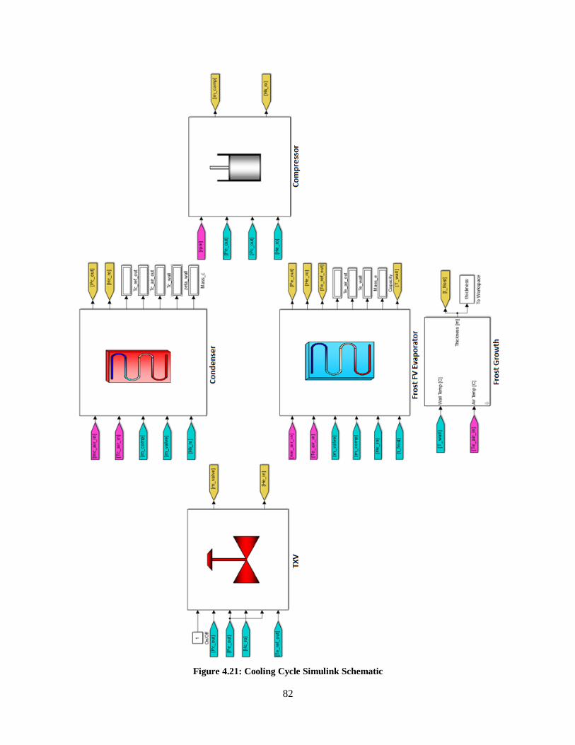
82

Figure 4.21: Cooling Cycle Simulink Schematic

83

4.5.1.1 Evaporator

The image below displays the frost finite volume evaporator as used in full cycle implementation. On

the left are block inputs, designated by a series of “from” tags. Air mass flow and air inlet temperature are

set by the user. In this case, air inlet temperature has been set at 21.1˚C and mass flow at 0.121 kg/s. These

conditions are comparable to those seen in a small air conditioning unit. The remainder of the external

inputs seen in Figure 4.22 are signals routed from other cycle components, providing comparable

connectivity to that seen in physical applications. For instance, inlet mass flow and inlet enthalpy are based

upon outputs of the expansion device, while outlet mass flow is based upon compressor inlet conditions. A

demonstration of this is provided in Figure 4.21. Likely the most important input for this analysis, however,

is frost thickness. Its use as an input signal allows the desired ability to couple frost and evaporator

dynamics to be achievable. Previous sections have stressed the importance of the causal relationship

between frost growth and evaporator behavior. This sort of feedback loop can be applied through the use

of the frost growth block in unison with vapor compression system modeling. In order to achieve this, the

frost thickness input signal is routed from the output of the frost growth block seen in Figure 4.23. Note

that the evaporator shown here is the “unmasked” version of that shown in Figure 4.21, as it allows inlet

signal labels to be visible.

Figure 4.22: Full Cycle Frost Finite Volume Evaporator Simulink Block

84

Additional input parameters can be entered by double-clicking the block, as described previously. In

this case most of the input parameters are relatively unimportant as trend characteristics are desired rather

than the specifics regarding operating conditions of the system. Based on this intent, only three parameters

are of interest for the current study. In the “Evaporator Properties” tab of the frosted finite volume

evaporator, the number of fins chosen was 700 and evaporator length was specified at a value of 7 m. This

allowed for a fin spacing value of 10 mm to be used in the frost growth block. Additional geometry

specifications are as seen in Figure 4.15. The last parameter of interest for simulation is the desired number

of volumes into which the evaporator will be divided. For all simulation data presented in Section 4.5, this

value was set to the maximum number of volumes (10) to obtain the greatest amount of accuracy. Entry

for this value can be found in the “Simulation” tab.

Outputs of this block can be seen on the right hand side of Figure 4.22. “Goto” tags are used to route

outlet refrigerant behavior to other components in the cycle, such as outlet pressure and enthalpy. These

outlet values are then routed for use as inputs to the compressor component. The last input seen here is a

set of evaporator wall temperatures, each corresponding with one of the ten total evaporator volumes

specified in the “Simulation” tab. In addition to the “goto” tag used for wall temperature, the set of final

wall temperatures is saved to the workspace to be used in defrost simulation. Lengthier discussion

regarding defrost will be conducted in later sections.

4.5.1.2 Frost Growth

To complete the feedback loop and causal relationship between frost and evaporator behavior,

evaporator wall temperature outputs are used as input signals for the developed frost growth block. This

means that behavior associated with system operation is able to affect the dynamics of frost growth, while

the amount of growth is similarly capable of affecting evaporator dynamics. This is a key feature that

separates modeling efforts proposed in this thesis to many past works. Similar to the previously discussed

set of evaporator wall temperatures output by the finite volume evaporator block, the final thickness output

value will also be saved to the workspace for later use in simulation of operation during defrost.

Figure 4.23: Full Cycle Frost Growth Simulink Block

85

For simplicity, input parameters used in the full cycle implementation are those seen in Figure 4.2, with

relative humidity set at 90%, fin pitch at 10 mm, and air velocity at 1 m/s. Air inlet temperature is equivalent

to that used as an input to the evaporator block, which was set at 21.1˚C.

4.5.1.3 Cooling Cycle Simulation Results

As a means of providing a comparison of current Thermosys™ modeling and those proposed in this

thesis, a total of three simulations were run. In the first simulation, the existing Thermosys™ finite volume

evaporator was used. In the following analysis, this model will be considered the “baseline”. As was

brought up in Section 4.4.1, upon applying changes for providing surface efficiency estimations, it was

determined that current Thermosys™ modeling does not account for any sort of overall surface efficiency

in utilizing the NTU method for evaluating air side heat transfer coefficients. Since in the case of the frosted

model, fins are a necessary input, this allows for the ability to account for surface efficiencies for both

frosted and unfrosted conditions for a finned system. The second test case resultingly made use of the

finned surface efficiency without the inclusion of frosting effects. Finally, the last simulation utilized the

model approach proposed in this thesis, allowing for frost growth and evaporator dynamics to be dependent

on one another. Note that in this third test case, surface efficiency was evaluated based on the unfrosted

finned model when no frost was present on the system. A summary of the stated test cases and their

respective efficiency effects can be found in Table 4.2.

Table 4.2: Full Cycle Implementation Model Comparison

Model Fin Effects Frost Effects

Baseline

Finned Unfrosted X

Frosted (This Thesis) X X

Operating conditions were kept uniform in all cases to allow for direct comparison, with simulations

being run for a 4 hour time period. For both of the unfrosted systems (baseline and finned), a frost thickness

of 0 mm was used as an input throughout the entirety of the simulation. Findings then demonstrate the

difference between operation under optimal conditions and those in which system degradation is

considered. Assessment of these behaviors also shows the need for a tool that accounts for such variations.

The evaporator wall temperature distribution associated with operation under frostless conditions for

current Thermosys™ modeling techniques (baseline) can be seen in Figure 4.24. Individual volumetric

wall temperatures are denoted by differing line color and/or type. Sections closest to the evaporator

entrance (1) are located further down in the plot, as refrigerant entrance temperatures should be lower than

those closest to the exit (10) while operating in refrigeration. Note that two of the wall temperatures

indicated in this diagram are below freezing, meaning that frost growth would be likely in application. The

plot indicates that steady state conditions are reached almost immediately, and remain constant through the

entirety of the simulation in the assumed absence of frost.

86

Figure 4.24: Cooling Baseline Evaporator Wall Temperature vs. Time

A similar result was obtained for the case in which only fins were considered, while still neglecting the

possibility of frost accumulation. The results of this can be seen in Figure 4.25. It is assumed here that the

surface efficiency drop associated with fins causes a decrease in the overall cooling capacity. Effects of

this will be seen in later discussion. This result can also be deduced from the fact that all wall temperatures

lie at least slightly below those of the baseline evaporator.

Figure 4.25: Cooling Finned Unfrosted Evaporator Wall Temperature vs. Time

For consideration of frost growth during system operation, evaporator inputs used are as described

before, with input frost thickness being the output of the frost growth block. Again, this also means that in

0 1 2 3 4

-5

0

5

10

15

20

Time [h]

Evap

ora

tor

Wall T

em

pera

ture

[C

]

1

2

3

4

5

6

7

8

9

10

0 1 2 3 4-10

-5

0

5

10

15

20

Time [h]

Evap

ora

tor

Wall T

em

pera

ture

[C

]

1

2

3

4

5

6

7

8

9

10

87

order to complete the feedback system, evaporator wall temperatures are used as inputs to the frost growth

block. Figure 4.26 displays the effect coupling of frost and system dynamics has on output evaporator wall

temperatures.

Figure 4.26: Cooling Frosted Evaporator Wall Temperature vs. Time

In this case, five of the ten evaporator volumes have wall temperatures capable of producing frost by

the end of the simulation. After the 4 hour simulated time frame and about 5 min of real time results show

final frost thickness values of 5.325 mm, 5.236 mm, 3.735 mm, 0.8635 mm, and 3.57*10-5 mm in segments

1, 2, 3, 4, and 5 respectively. It is interesting to note that each these segments start out at the same

temperature as those seen in Figure 4.25 and gradually begin to deviate in a decreasing manner. Behavior

such as this is expected due to the characteristic performance degradation of systems operating under

frosting conditions. This deviation is almost immediate, as frost growth ensues early on in the refrigeration

cycle due to surface temperatures starting out below 0˚C. Unlike the case before in which evaporator wall

temperatures remained constant throughout the simulation, the diagram above indicates that all wall

temperatures exhibit a drop with time. The impact of which is greater in some volumetric sections than

others. This supports the fact that less thermal energy removal is possible as frost builds up, resulting in

the decrease of refrigerant temperatures.

A direct comparison of system outputs, including cooling capacity, air outlet temperature, refrigerant

outlet temperature, and refrigerant outlet pressure, can be found in Figure 4.27 through Figure 4.30. The

baseline model is designated by a solid line, unfrosted finned model by short-dashed line, and the frosted

finned system is displayed as a long-dashed line. In all cases, the unfrosted systems remain constant

throughout the simulation, as degradation of system performance does not occur when frost is not taken

0 1 2 3 4

-20

-15

-10

-5

0

5

10

15

20

Time [h]

Evap

oeato

r W

all T

em

pera

ture

[C

]

1

2

3

4

5

6

7

8

9

10

88

into account. Note that cooling capacity remains constant at a value of 853.6 W for the Thermosys™ model

and at a slightly lower 840.1 W for the unfrosted finned model when fin effects are accounted for. This is

a result of the decrease in overall surface efficiency and can be seen in Figure 4.27. The frosted model

cooling capacity seems to start out at about the position of the solely finned model, which would make

sense as this is how it is treated in the absences of frost. However, a gradual drop in capacity is noticeably

visible soon after the simulation is initiated. This is likely due to the fact that upon initiation, there are

already a few surface temperatures that lie below the freezing point. Therefore, frost growth begins almost

immediately. The degradation of system performance appears to be somewhat exponential as the provided

cooling capacity exhibits a dramatic drop between 3 and 4 hours of operation. An overall drop of about

179.1 W can be seen when frost is accounted for, corresponding to a 21.3% decrease after 4 hours of

operation.

In the original frosted system data there are two visible jumps in the cooling capacity versus time plot

(Figure E.3). These deviations occur when a new evaporator volume has met appropriate frosting

conditions and frost growth has been initiated. MATLAB code is written to evaluate frost growth as

somewhat of an on/off switch. This means that frost growth is assumed to either be occurring or not over

the coil segment. The numerical simulation treats this sudden triggering of frost growth as an impulse,

which corresponds to visible aberrations. Behavior is however able to return to expected behavior soon

after. Data presented in Figure 4.27 has been filtered to reduce the effect of the associated disturbance on

simulation outputs. Filtering was conducted through the use of a Butterworth low pass filter through which

cooling capacity outputs were sent. Specific filter block inputs and a comparison of filtered to unfiltered

data can be found in Appendix E.

Figure 4.27: Cooling Cycle Cooling Capacity vs. Time (Filtered)

0 1 2 3 4

650

700

750

800

850

Time [h]

Co

olin

g C

ap

acit

y [

W]

Baseline

Finned Unfrosted

Frosted (Filtered)

89

Air outlet temperature was the only other parameter that exhibited similar deviations to those seen in

cooling capacity. Unfiltered air outlet temperature results can be found in Figure E.6. Filtered air outlet

temperature data as a function of time is plotted in Figure 4.28 and was obtained through the use of an

identical filter to that used for cooling capacity data. The same filter was used in each instance for both

cooling and defrost as a means of simplification. Users may however select and tune filters as desired to

reduce the effect of the indicated deviations.

At steady state, the unfrosted systems provide an outlet air temperature of 14.09˚C and 14.2˚C for the

baseline and finned models, respectively. However, when frost is considered, air outlet temperature

exhibits a gradual increase. Less thermal energy can be removed from the environment as the above cooling

capacity is reduced, resulting in an overall air outlet temperature increase of 1.47˚C after 4 hours of

operation in cooling.

Figure 4.28: Cooling Cycle Air Outlet Temperature vs. Time (Filtered)

Also a consequence of the aforementioned reduced cooling capacity, outlet refrigerant temperature has

the inverse effect of that exhibited by air outlet temperature. Figure 4.29 indicates that for the baseline

model, steady state operation produces an outlet refrigerant temperature of 14.74˚C. Slightly lower is that

of the unfrosted finned model, for which a steady state temperature of 14.2˚C was found. Accounting for

effects occurring as a result of operation under frosting conditions, however, the model estimates a final

outlet temperature of 7.802˚C. This corresponds to an overall temperature drop of about 6.398˚C over the

4 hour simulated timeframe.

0 1 2 3 414

14.2

14.4

14.6

14.8

15

15.2

15.4

15.6

15.8

16

Time [h]

Air

Ou

tlet

Tem

pera

ture

[C

]

Baseline

Finned Unfrosted

Frosted (Filtered)

90

Figure 4.29: Full Cycle Refrigerant Outlet Temperature vs. Time

Figure 4.30: Cooling Cycle Refrigerant Outlet Pressure vs. Time

The last parameter considered in the comparison of system dynamics is refrigerant outlet pressure. In

the absence of frost and fins, a constant refrigerant outlet pressure of 372 kPa was predicted. Outlet pressure

displays a decrease with time when frost is considered due to the consequent increased frost thickness.

Temperature and pressure are assumed to be correlated, so the observed decrease in outlet pressure

corroborates temperature findings above. In all, when frosting effects are considered, refrigerant outlet

pressure is about 60.6 kPa lower than that of an unfrosted finned system, operating at 367.1 kPa and 65.5

0 1 2 3 4

8

9

10

11

12

13

14

15

Time [h]

Refr

igera

nt

Ou

tlet

Tem

pera

ture

[C]

0 1 2 3 4300

310

320

330

340

350

360

370

Time [h]

Refr

igera

nt

Ou

tlet

Pre

ssu

re [

kP

a]

Baseline

Finned Unfrosted

Frosted

91

kPa lower than that of current of the baseline modeling prediction. This corresponds to a final pressure

output of 306.5 kPa after 4 hours.

Much like the sensitivity analysis provided in Section 2.2 for the developed frost melt model, one will

be presented here in regard to frost growth. Findings have been presented in this section due to the desire

to quantify how sensitive both frost growth and performance are to changes in various growth parameters.

A new full cycle model was run to serve as the baseline model for sensitivity analysis. Increases of 10%

for each parameter were then conducted on an individual basis to allow effects to be isolated. Changes in

fin pitch and air velocity are relatively straightforward. Note that changes in fin pitch also require that

geometry changes be made to the evaporator model as well. Increased temperature difference however can

result from changes in three different parameters, those being air temperature, relative humidity, and

evaporator surface temperature. Relative humidity is the only parameter of the three in current modeling

that is not also used as an input to the finite volume evaporator block and will therefore be used to incur the

10% increase on temperature difference.

Table 4.3 displays baseline parameter values alongside those associated with a 10% increase. Second

from the right are the final resulting cooling capacity values for increases in the designated parameter after

a 4 hour operation period in cooling. The baseline temperature difference featured in the following table is

the result of an air temperature of 21.1˚C, relative humidity of 80% (DP of 15.90˚C), and evaporator surface

temperature of -8.853˚C. Evaporator surface temperature was assumed to be that closest to the evaporator

inlet as it provided the greatest overall temperature difference. The indicated 10% increase in temperature

difference is the result of an 89% relative humidity value. Using the baseline parameters, the evaporator

was still capable of providing 785.4 W of cooling. When frost is not considered, the system is estimated to

provide 840 W of cooling (with fins).

Table 4.3: Frost Growth Sensitivity Analysis

Parameter Baseline 10%

Increase

Final Cooling

Capacity [W]

Percent

Change [%]

Temperature Difference [C] 24.688 27.1568 722 -8.072319837

Fin Pitch [mm] 10 11 795.8 1.32416603

Air Velocity [m/s] 1 1.1 789.4 0.509294627

The percent change in cooling capacity associated with each increase can be seen in the furthest right

column. Percent change values were again normalized to show the effect of each relative to the others.

Magnitude and direction of each effect are visible in Table 4.3, with findings indicating that temperature

difference has a largely negative impact. Increases in fin pitch and air velocity actually increase the amount

of cooling capacity achievable after 4 hours of operation. Figure 4.31 displays the normalized magnitudes

of the effect each parameter has on cooling capacity.

92

Figure 4.31: Normalized Percent Cooling Capacity Change Magnitude by Parameter

Temperature difference seemingly has the greatest overall effect, followed by fin pitch. This is

unsurprising in that when the surface temperature is well below that of the dew point, frost growth is more

likely. Trends provided in Chapter 2 indicate that frost thickness decreases when fin pitch is increased,

which may account for the indicated increase in cooling capacity resulting from a 10% increase in fin pitch.

Cooling capacity appears to only be minutely sensitive to changes in air velocity. Correlations provided in

Appendix A suggest that if air velocity were instead decreased by 10%, the designated sensitivity would be

relatively higher. This seems to be due to the fact that when air flow is slower, frost thickness is

correspondingly thicker after a given period of time. An additional test case was run to prove this

hypothesis. When air velocity was instead decreased by 10% (0.9 m/s), the simulation was terminated prior

to finishing the 4 hour timeframe because frost blockage had begun to inhibit air flow. Sensitivity to this

10% decrease would therefore have been much higher than that found for a 10% increase. It is therefore

important to acknowledge that the sensitivity of cooling capacity to each of the parameters of interest will

also be subject to associated trends provided in Chapter 2 and Appendix A. However, temperature

difference will likely have the greatest influence in most cases as it plays a more critical role in determining

how much moisture content may be removed from the air and ultimately collected on heat transfer surfaces.

4.5.1.4 Conclusion

Overall, the results presented in this section indicate findings similar to those common in application,

with visibly decreasing cooling capacity as well as the resulting increase in air outlet temperature and

pressure drop across the evaporator occurring during operation under frosting conditions. It should be noted

that parameters used in this investigation are similar to those that might be seen in a small air conditioning

unit (less than 1 kW of cooling). Visible trends presented here are appropriate, however, the magnitude of

93

individual system degradation during cooling will be dependent on specified geometry and operating

conditions.

Based on data presented by Reindl [32], performance degradation within the first 10 hours of operation

is relatively minute (about 1%) even on a much larger system (110 kW). Significant deviation (about 20%)

is not actually seen until about 41 hours of operation time. Similar trends are seen here in that system

degradation appears slow at first and seems drop at a more rapid rate as more time passes and more frost is

able to build up. The reason cooling capacity associated with the system being used in this analysis seems

to decrease relatively quickly (4 hours) is because air temperature was relatively high and resultingly had

more moisture content. Frost accumulation was therefore much more rapid than that presented by Reindl

in which air inlet temperature was -28˚C and evaporator surface temperature was -34.4˚C.

Caution must be taken in many applications to prevent too much cooling capacity loss prior to operation

in defrost, because such operation incurs an additional heating load on the region being cooled. This means

that defrost must start prior to environmental temperatures being able to experience a significant rise. In

the example presented here, defrost would likely be necessary prior to actually reaching the end of the 4

hour timeframe in order to prepare for the anticipated negative impact associated with operation in defrost.

In general, defrost decisions will be based upon specific temperature tolerances and how strict those

tolerances are. For instance, systems used for maintaining human comfort are likely much more lenient in

terms of temperature tolerances than food storage applications, where failure to meet certain storage

requirements could be detrimental. Hot-gas defrost modeling will be discussed in the next sub-section.

4.5.2 Hot-Gas Defrost

Unlike the cooling cycle discussed in Section 4.5.1, operation in hot-gas defrost consists of hot,

compressed refrigerant being diverted directly through the evaporator rather than the condenser, as is done

in operation during cooling. During defrost, the evaporator resultingly behaves as a condenser, allowing

surface temperatures to reach values high enough to eliminate the accumulated layering for frost. As such,

hot-gas defrost in Simulink consists of looped connectivity between only three components, those being an

evaporator component, compressor component, and expansion valve. Operating conditions for the

simulated hot-gas defrost configuration can be seen in Table 4.4. A schematic of the model can be found

in Figure 4.32.

Table 4.4: Hot-Gas Defrost Operating Conditions

Parameter Value Units

Refrigerant R404A

Evaporator Pressure 1475 kPa

Compressor Speed 1500 rpm

EEV Stroke Fraction 0.25 -

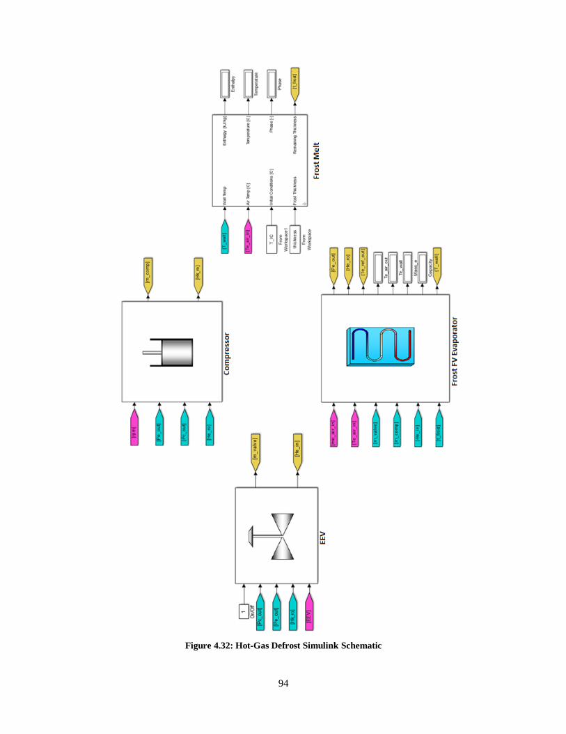
94

Figure 4.32: Hot-Gas Defrost Simulink Schematic

95

As indicated in previous sections, visible trend characteristics are of greatest interest for the time being,

rather than system specific data. In-depth details about simulation settings will therefore not be addressed

in this documentation. Though individual component specifications will not be discussed in great detail,

complementary discussion regarding associated settings will be conducted in the following sub-section as

frost melt modeling is a key component of the ideas presented in this thesis. Note that the evaporator used

in simulating defrost behavior will be identical to that used during cooling. It will be assumed that fans

will be in the off position during defrost as is common in hot-gas defrost. Air mass flow rate will then have

a value of 0 kg/s. For additional information on evaporator settings, please refer to Section 4.5.1.1.

4.5.2.1 Frost Melt

In this case, in order to complete the feedback loop and causal relationship between frost and evaporator

behavior, evaporator wall temperature outputs are again used as input signals for the developed frost melt

block. Similar to the method used in representing a cooling cycle, remaining thickness outputs of the frost

melt block (Figure 4.33) are used as frost thickness inputs to the evaporator block seen in Figure 4.22. This

feedback configuration allows melt modeling to influence evaporator dynamics, while melt behavior is

similarly affected by system dynamics. Where in the cooling cycle, the set of final evaporator wall

temperatures and final frost thickness values were saved to the MATLAB workspace, modeling of operation

in hot-gas defrost allows for these saved values to then be called from the workspace and instead be used

as frost melt block inputs (Figure 4.33).

Figure 4.33: Defrost Cycle Frost Melt Simulink Block

96

Parameter settings for the frost melt Simulink block were identical to those displayed in Figure 4.7 and

Figure 4.8 for frost and liquid properties, respectively. Heat exchanger geometry inputs were be based

upon designated evaporator geometry, which can be seen in Figure 4.15. The number of evaporator

volumes used in modeling of the defrost cycle must be equivalent to the designated number of volumes for

the cooling cycle, so this values has again been set at a value of 10

4.5.2.2 Hot-Gas Defrost Simulation Results

Similar to the analysis conducted for the cooling cycle, discussed in Section 4.5.1, analysis of the hot-

gas defrost process will draw comparisons between three different modeling methods. First, current

Thermosys™ modeling techniques will be discussed. This model will again be designated as the “baseline”

model. Then, an unfrosted, finned model will be addressed, to be followed by the proposed frosted, finned

model. Please refer to Table 4.2 for more information on how each of these modeling methods differ.

Three simulations were again run, each with identical input parameters to allow for direct comparison of

results. For the unfrosted models (baseline and finned), frost thickness was again held at a value of 0 mm

throughout the duration of the defrost simulation.

Figure 4.34: Defrost Baseline Evaporator Wall Temperature vs. Time

The evaporator wall temperatures associated with operation under frostless conditions for the baseline

model can be seen in Figure 4.34. Individual volumetric wall temperatures are again denoted by differing

line color and/or type. Note that the each volumetric temperature is denoted as before. In this case, the

inlet volume (1) is at a higher temperature than the outlet volume (10), while during cooling, the opposite

was true. This decreasing temperature trend along the length of the evaporator coincides with heat rejection

0 5 10 15 20 25 3021.45

21.5

21.55

21.6

21.65

Time [min]

Evap

ora

tor

Wall T

em

pera

ture

[C

]

1

2

3

4

5

6

7

8

9

10

97

due to operation in defrost, rather than absorption. This effect will become much more evident in later

discussion regarding heating capacity.

Figure 4.35: Defrost Finned Unfrosted Evaporator Wall Temperature vs. Time

Similar findings were observed for the case in which fins were considered, while still neglecting the

presence of frost. Wall temperature distribution results are displayed in Figure 4.35. With the addition of

a surface efficiency term associated with finned surfaces, the amount of heat transfer between the refrigerant

and environment is decreased, resulting in a slight increase in wall temperatures relative to the baseline

case. Though these differences are somewhat difficult to see, as they are relatively minute, the heating

capacity associated with these two cases will provide a more visible contrast and will be addressed later.

Lastly, evaporator wall temperature distribution during hot-gas defrost for the frosted model can be

seen in Figure 4.36. Where operation in cooling produced temperatures ranging between about -10˚C and

21˚C, temperatures seen during defrost range between about 21.45˚C and 21.7˚C. Upon initiation of the

defrost cycle, temperatures can visibly be seen rising on the left hand side as the system switches from

cooling to defrost. In all ten volumes, temperatures show a gradual decrease between the 3 min mark and

15 min mark. At this point, temperatures exhibit a bit of a drop-off, signifying the full elimination of one

of the sections of frost. Recall that in the last section, there were five volumes of the evaporator in which

wall temperatures were below the freezing point at the end of the 4 hour simulation period. In defrost, there

are similarly five drop-off points signifying the complete elimination of each of the five frost layers. Two

of these frosted segments exhibit drop-offs very early on in the simulation as they had very little frost. In

these early stages (0 min to 5 min), temperatures are still rising, so these disturbances are not as noticeable.

This results in only three of these drops being evident in both wall temperature and heating capacity plots.

0 5 10 15 20 25 3021.45

21.5

21.55

21.6

21.65

Time [min]

Evap

ora

tor

Wall T

em

pera

ture

[C

]

1

2

3

4

5

6

7

8

9

10

98

Figure 4.36: Defrost Frosted Evaporator Wall Temperature vs. Time

The evaporator, now acting similar to a condenser, is not able to reject as much thermal energy as a

result of the thermal resistance provided by the frost layer present on the system. With the removal of this

layering, the evaporator is capable of achieving a higher heating capacity (Figure 4.37), or rejection of

thermal energy. The impact of this can be seen in the resulting decrease of both refrigerant and evaporator

wall temperatures.

Figure 4.37: Defrost Cycle Heating Capacity vs. Time (Filtered)

A comparison of the heating capacity provided by each of the individual models as a function of time

is shown in Figure 4.37. Data has again been filtered using the Butterworth filter discussed in Appendix E

0 5 10 15 20 25 3021.45

21.5

21.55

21.6

21.65

Time [min]

Evap

ora

tor

Wall T

em

pera

ture

[C

]

1

2

3

4

5

6

7

8

9

10

0 3 6 9 12 15 18 21 24 27 300

1

2

3

4

5

6

Time [min]

Heati

ng

Cap

acit

y [

W]

Baseline

Finned Unfrosted

Frosted (Filtered)

99

to reduce the triggered response resulting from a new layer of frost has being shed. Figure 4.37 has been

plotted using filtered frosted system data, while Figure E.9 displays the same plot instead using unfiltered

data. Additionally, Figure E.10 and Figure E.11 provide a direct comparison of filtered and unfiltered data.

The unfrosted baseline model appears to have the highest heat transfer capability, providing about 5.428

W, since it is uninhibited by a surface efficiency term. At a slightly lower 5.349 W is the unfrosted finned

model, for which the associated overall surface efficiency has been included. The incurred decrease in

overall surface efficiency causes the resulting decrease in the maximum achievable heat transfer. As a

reflection of behaviors seen in evaporator wall temperatures associated with the frosted model

configuration, Figure 4.37 also displays the associated heating capacity as a function of time. The plot

again displays three distinctive peaks, indicating the jump in heating capacity that the system provides as a

result of a new layer of frost being shed. Note that this is again due to the fact that the other two frosted

segments occurred very early on in the simulation while behavior is still very dynamic. Figure 4.37 has

been zoomed in to provide a better visual of these three described increases in capacity, however a full plot

can be found in Figure E.10. As would be expected, the frosted model ultimately converges to the heating

capacity associated with the unfrosted finned model.

An additional output of time to defrost is sent to the workspace so that users may determine how long

the simulation estimates it took the system to fully remove the frost layering. This can be particularly

helpful in cases where a timer-based defrost is utilized. At the beginning of simulation, the user must

designate a run time. For a timer-based system, the timer setting would likely be entered. This time to

defrost output then has the potential to provide some insight into how long defrost should actually last, as

well as the amount of energy lost as a result of running unnecessarily. For example, the simulation used in

past sections to simulate Hoffenbecker’s experimental work was set to run for a total of 45 min, as this is

how long timer-based experimental system was set to run in defrost. The time to defrost output was then

able to indicate that although the system ran for the duration of the defrost cycle, frost removal was

completed after only 11 min and 4sec. For the example provided in this section, defrost was estimated to

be complete after about 24 min. This finding is supported by Figure 4.37, as this is at the point that the

final rise in cooling capacity occurs.

4.5.2.3 Conclusion

Discussion in this section focused on the modeling of hot-gas defrost and the resulting impact on system

operation. In all, presented findings demonstrate trends frequently seen in application. In initial phases of

defrost, when the majority of the frost accumulation is still present, the thermal resistance and energy

consumption due to phase change reduce the amount of loading put on the environment. Over time and as

the frost growth is gradually removed, this loading begins to increase to a point at which defrost is no longer

100

contributing to phase change. Instead thermal energy is purely being used to heat the environment that is

desired to be cooled. Figure 4.37 demonstrates this, and provides a perfect example as to why defrost

running significantly longer than necessary could incur a significant loading that the system will then have

to compensate for during operation in cooling. A tool such as the one introduced for this thesis could,

therefore be used to aid in reducing the likelihood of this excessive operation in defrost.

4.6 Conclusion

This chapter details the steps taken as a means of applying frost growth and melt modeling techniques,

described in previous chapters, to the currently existing Thermosys™ Simulink toolbox. Through the use

of an already established modeling tool, implementation of frost behavior modeling discussed in this thesis

could easily be coupled with system operational dynamics during operation in both cooling and defrost; an

element that is missing from published modeling efforts to date. As such, this implementation was critical

to demonstrating the utility of modeling methods described in this thesis and providing a desired broader

impact.

Discussion begins with the introduction of Thermosys™ and its use as a tool for simulating the

dynamic behavior of vapor compression systems. Sections 4.2 and 4.3 present the individual Simulink

blocks created for executing previously described frost growth and frost melt modeling techniques,

respectively. Necessary input parameters as well as output values are addressed and demonstrated through

the use of an example standalone simulation for each case.

In addition to solely converting suggested modeling approaches for compatibility in Simulink, some

changes also had to be made to the evaporator component currently used in Thermosys™. These alterations

are discussed in Section 4.4. Current Thermosys™ modeling techniques make use of the NTU method in

evaluating heat transfer, with an assumed surface efficiency of 100%. In the presence of both fins and frost,

however, this efficiency is significantly reduced, so modifications to allow for this reduction in efficiency

are addressed in Section 4.4.1. With an added input of frost thickness and evaporator wall temperature

output, the resulting frosted finite volume evaporator was introduced, and standalone simulation results

presented.

Through the use of these three key components in unison with compressor, condenser, and expansion

device components currently available in Thermosys™ a full vapor compression cycle was demonstrated.

Two separate Simulink models were produced to achieve this, one consisting of system configuration in

cooling (evaporator, compressor, condenser, expansion device and frost growth components), while the

other represented operation in defrost (evaporator, expansion valve, compressor, and frost melt

components).

101

Findings for each of these modes of operation were presented individually, with resulting trends being

comparable to those frequently seen in physical application. Analysis of operation in cooling indicated that

with the inclusion of frosting effects, system degradation was visible. As frost thickness increased, the

resulting system dynamics demonstrated a decreased cooling capacity. With this reduction in the system’s

ability to remove heat from the environment, air outlet temperature accordingly displayed a visible increase.

Conversely, both refrigerant outlet temperature and pressure indicated a decrease, correlating to greater

pressure drop across the evaporator. Operation in defrost, however, produced the opposite effect on heat

transfer, since with the reduction in frost, the amount of heat transfer the system was capable of providing

increased. This gradual increase in heat capacity was also evident in the observed evaporator wall

temperature distribution, with temperatures exhibiting a decrease as more and more frost was shed. The

results presented in this section and their reflection of physical trends are evidence that models produced

for this thesis can improve the predictive capability of current vapor compression system modeling

methods, particularly in cases where frosting conditions are present.

Though this idea has been reiterated time and time again throughout this section, it is critical to keep in

mind that the results provided in this section are meant purely as a demonstration of dynamic system

performance under frosting conditions. One of the key benefits of being able to build off of the already

established Thermosys™ library is that simulation allows for user defined system geometry and input

values, allowing for somewhat universal applicability. The results shown here are therefore meant to show

general trends that are expected to be seen for all simulated cases in which system operation is occurring

under frosting conditions. Specific operating conditions are not discussed in detail in this section, as

variations in user specifications will likely cause consequential differences in the extent system

performance is impacted by the insulating effects exhibited by frost growth. Without experimental data for

comparison, or the capacity to collect such data at the time of this writing, the demonstration of performance

trend characteristics and the fact that exhibited behaviors align well with physically observed trends are of

primary importance here.

102

Chapter 5

Conclusion

5.1 Summary

The discussion provided in this thesis details the steps taken in model development and implementation

of frost growth and melt behavior and the resulting effect on refrigeration system dynamics and

performance. Initially, background was provided on the negative side effects associated with frost

accumulation on evaporators operating under frosting conditions and the resulting need for system defrost.

As current defrost strategies do not gage the amount of frost on heat transfer surfaces, a model-based

approach was chosen in an effort to provide a means of predicting frost growth, its effect on system

performance, and the corresponding time necessary for defrost. A major benefit of this type of strategy is

that information may be made available a priori.

Modeling of the frost growth and melt processes were then discussed in Chapter 2. As a process on the

order of hours, frost growth modeling was chosen to be correlation based. On the other hand, frost melt is

on the order of minutes, so a first principles approach was taken in order to attempt to capture its very

transient nature. Each model was then individually validated as a standalone model, as described in Chapter

3, with findings showing good predictive capability. Less than 15% maximum deviation from published

findings was determined for frost growth. Defrost duration was estimated at 11 min and 4 sec in simulation,

with published findings suggesting a qualitative defrost time lying between 10 and 14 min.

In addition to being able to predict frost behavior, a critical objective of this thesis is the ability to

couple this predicted behavior with system operational dynamics; a feature that is commonly unaccounted

for in published findings to date. Implementation of developed frost growth and melt modeling into the

currently existing Thermosys™ framework is therefore discussed in Chapter 4. Through this

implementation, the causal relationship between evaporator performance and frost behavior could be

represented, such that frost dynamics not only affect system performance, but system dynamics similarly

impact frost behavior.

103

Integration of proposed modeling methods required that Simulink models be created, for which

standalone results are discussed. Similarly, full vapor compression cycle modeling was completed in two

parts, those being a cooling cycle and hot-gas defrost cycle. Results provide similar trends to those seen in

application, with cooling capacity decreasing at a more rapid rate over time and air outlet temperature

consequently increasing. Operation under hot-gas defrost conditions displayed the gradual recovery of heat

transfer with the removal of collected frost. In this case, the increased heat transfer correlated to an observed

increase in heat capacity and corresponding decrease in refrigerant temperature as a result of operation in

defrost.

Findings in both cases provide a comparison between current Thermosys™ modeling (baseline), in

which surface efficiency is taken to be 100%, an unfrosted finned model, and the proposed modeling

method in which frost behavioral effects are acknowledged. Observed deviation of system performance

from the optimal case, in which system operation is uninhibited by the presence of frost, is able to provide

evidence that modeling methods developed in this thesis have the potential to provide more accurate insight

into system performance when operating under frosting conditions. With this gained insight, more

knowledgeable decision making can be used in evaluating both when defrost should be triggered as well as

its duration, all of which can be conducted a priori.

5.2 Future Work

The discussed modeling and implementation techniques presented in this thesis demonstrate the utility

of frost growth and melt modeling, as well as how a model-based approach can provide information

necessary for improving operational efficiency commonly associated with operation in defrost. Though

modeled trends indicate consistency with those commonly seen in application, there are still a few areas in

which further improvement can be achieved. These key areas are discussed in the following subsections in

order of priority, as defined by the author.

5.2.1 Model Validation

Validation for both frost growth and frost melt models discussed in Chapter 2 is demonstrated in

Chapter 3 for each independent model as a standalone component. Though demonstrated validation efforts

do provide fair predictive capability, additional test cases would likely further aid in substantiating

modeling potential.

Furthermore, in the absence of an experimental system, validation efforts have not confirmed system

level operation or evaporator performance under frosting conditions. Results presented in Chapter 4 exhibit

trends similar to those seen in application and as such, indicate modeling ability on a qualitative level.

Quantitative analysis, however, is still necessary to fully demonstrate that experimentally observed

104

behavior is comparable to the observed simulated behavior. As a result, steps moving forward should

primarily be aimed at development of an experimental system for data collection or acquiring data for

comparison. This will be a key step moving forward as a means of fully establishing the utility of the tools

developed for this thesis.

5.2.2 Frost Growth Modeling

In regard to frost growth modeling, one of the biggest drawbacks of the current means in which growth

correlations are developed is that they are only valid within a relatively narrow range of values. For

instance, relative humidity values must lie between 70% and 90% for existing correlations to be applicable.

Though an experimental system was not available in conducting work for this thesis, collecting

experimental data for a wider range of ambient and operating conditions would allow for more accurate

correlations and predictive capability.

In addition to the possibility of obtaining improved correlations, development of a more first principles

based model may provide greater insight into the process as a whole. A correlation based approach was

utilized in this thesis as a means of simplifying the extensive process associated with frost growth as

computation of transients over such a long period of time would have likely required a much greater amount

of computational time and power. Greater understanding of the physics behind this behavior could however

provide greater understanding of actual frost growth behavior, as well as why the aforementioned

correlations exist. It may be possible that with a greater comprehension of the associated physics,

parameters similar to those used in this thesis could still be identified. As a result, a first principles based

model would be suggested moving forward, particularly if greater accuracy is desired. Some of the work

currently being done at the University of Illinois at Urbana-Champaign is aimed at making use of modeling

to evaluate the amount of water content removed from flowing air during the cooling process. Further work

could therefore make use of such capability to aid in the development of a more first principles based growth

model.

Though the current model developed for this thesis does take into account the effect air velocity has on

the frost growth process, as well as the corresponding convective heat transfer in the presence of frost, it

does not incur any effect on flow velocity across the heat transfer surface. With increased frost growth, it

is not uncommon for air flow through the evaporator to decrease as a result of frost blockage. Correlations

presented in the Chapter 2 are based upon growth data, so these effects are likely already included in

determining frost thickness as a function of time, however, corresponding outcomes in evaporator

performance are not incorporated. Although this decrease in air flow will likely induce a slight decrease in

cooling capacity, current modeling does provide a fair estimation. This is because the primary contributor

105

to deteriorated performance comes as a result of thermal resistance associated with the frost layer, which is

reflected in model implementation. Nonetheless, with greater knowledge of evaporator geometry and

variation in air flow as a result of frost growth, potentially greater accuracy can be achieved.

5.2.3 Model Implementation and Energy Management

The means of model execution discussed in this thesis requires that operation in modes of refrigeration

and hot-gas defrost be conducted in two separate Simulink models. Though modeling as currently applied

provides beneficial knowledge into system operation under frosting conditions and associated frosting

behavior, further advancements can be made in modeling of such processes by allowing for a single model

in which functionality allows for simulation in both modes of operation. A single model would allow for

ease of switching between operational modes, providing the ability to efficiently conduct system studies to

evaluate which combinations of refrigeration and defrost provide the greatest efficiency. For instance,

whether more frequent and shorter defrosts are more efficient than less frequent defrost cycles occurring

over a longer timeframe.

In addition, allowing for such switching in conjunction with the aforementioned studies would also

provide the ability to implement control mechanisms and defrost strategies aimed at improving system

performance. This could be accomplished by setting specified cooling capacity tolerances such that once

cooling capacity or air temperatures have reached designated operational tolerances, defrost operation

would be triggered and would then run for the necessary timeframe needed to fully eliminate the existing

frost layer. Estimations of this could be based upon the melt model proposed in this thesis. Once this

defrost is complete, the control algorithm may then allow cooling to resume. Similarly, controls can

potentially be developed in an effort to achieve minimum operational efficiency requirements.

Though relatively minor, additional improvements can also be made to input entry methods in an effort

to simplify use of the proposed tool. Currently, some parameters must be entered into multiple simulation

components used in a single Simulink workspace. Allowing users to only be required to enter these repeated

input parameters once would reduce the redundancy and prevent the possibility of users overlooking some

of these specifications. Additionally, modeling described in this thesis made use of data filters to reduce

the effect of numerical anomalies due to the presence of frost being considered either on or off. Further

work may be applied toward developing methods to eliminate these numerical effects or integrating filtering

into actual evaporator blocks.

106

Appendix A : Frost Growth Correlations

Figure A.1: Fin Pitch Coefficient 1

Figure A.2: Fin Pitch Coefficient 2

7 8 9 10 11 12-0.02

0

0.02

0.04

0.06

0.08

0.1

0.12

0.14

0.16

Fin Pitch (FP) [mm]

Fin

Pit

ch

Co

eff

icie

nt

1 (

C1F

P)

7 8 9 10 11 12-2

-1

0

1

2

3

4

5

6

7x 10

-6

Fin Pitch (FP) [mm]

Fin

Pit

ch

Co

eff

icie

nt

2 (

C1F

P)

107

Figure A.3: Velocity Coefficient 1

Figure A.4: Velocity Coefficient 2

1 1.5 2 2.5 3 3.5 4 4.5 5-1

-0.5

0

0.5

1

1.5

2

2.5

3

3.5

Air Velocity (V) [m/s]

Air

Velo

cit

y C

oeff

icie

nt

1 (

C1V

)

1 1.5 2 2.5 3 3.5 4 4.5 5-1.5

-1

-0.5

0

0.5

1

1.5

2

2.5x 10

-5

Air Velocity (V) [m/s]

Air

Velo

cit

y C

oeff

icie

nt

2 (

C2V

)

108

Figure A.5: Temperature Difference Coefficient 1

Figure A.6: Temperature Difference Coefficient 2

30 35 40 45 500.1

0.11

0.12

0.13

0.14

0.15

0.16

0.17

0.18

0.19

0.2

Dew Point to Surface Temperature Difference (dT) [C]

Tem

pera

ture

Dif

fere

nce C

oeff

icie

nt

1 (

C1d

T)

30 35 40 45 501.7

1.8

1.9

2

2.1

2.2

2.3

2.4x 10

-6

Dew Point to Surface Temperature Difference (dT) [C]

Tem

pera

ture

Dif

fere

nce C

oeff

icie

nt

2 (

C2d

T)

109

Appendix B : Preliminary Melt Modeling

Table B.1: Intermediate Node Energy Balance Coefficients

FFF 2

f

i

i

rw r

r

1 1 2

2 2

f

i i f

i

r ry r r

r

2

f

i

i

rz r

r

1 1

2 2

f n n n n

j i i i i i

i

r rm r h h r h h

r

TFF

0w 1 0.5( )2 2

mf i avg f i

f f i

r ry k r k k r

c r

2

f m

i

i

rz r

r

1 0.5( )2 2

n n nmf i i j avg f i i

f f i

r rm k r h h k k r h

c r

LFF

0.5( )

2

l f m

i

l f i

k k rw r

c r

1 0.5( )

2 2

mf i l f i

f f i

r ry k r k k r

c r

2

f m

i

i

rz r

r

1 1 20.5( )

2 2

n n n n

m i i i i latf i l f i

f i f f l l

h h h h hr rm k r k k r

r c c c c

LTF

0.5( )

2

l avg m

i

l avg i

k k rw r

c r

1y

0.5( )

2

f avg m

i

avg f i

k k rz r

c r

1 1 20.5( ) 0.5( )

2 2

n n

m i i latf avg i l avg i

avg i f l l

h h hr rm k k r k k r

r c c c

LLF

2

l mi

i

rw r

r

1 0.5( )

2 2

mf l i l i

l l i

r ry k k r k r

c r

0.5( )

2

f l m

i

l f i

k k rz r

c r

1 120.5( )

2 2

n n n n

m i i lat i if l i l i

l i f l l l l

h h h h hr rm k k r k r

r c c c c c

110

LLT 2

l mi

i

rw r

r

1 0.5( )

2 2

mavg l i l i

l l i

r ry k k r k r

c r

0z 10.5( ) 22 2

n n nmavg l i i lat l i i i

l l i

r rm k k r h h k r h h

c r

LLL 2

li

i

rw r

r

1 1 2

2 2

li i l

i

r ry r r

r

2

li

i

rz r

r

1 1

2 2

n n n nli i j i i i

i

r rm r h h r h h

r

Table B.2: Coil-Side Boundary Energy Balance Coefficients

Coil-FF

1

1 0.5( )f coil coil f coil

f f

y k r r k k rc r

1 2

f

coil

rz r

r

2 1

1

0.5( ) 2 2nn n

if coil coil f coil coil m

f f f

hh hm k r r k k r T T

r c c

Coil-TF

1y 1

0.5( )f avg

coil

avg f

k kz r r

c r

2 1

1

0.5( ) 0.5( ) 2 2n n

f avg coil coil avg coil m coil

avg f

h hm k k r r k k r T T

r c

Coil-LF

1

1 0.5( ) 0.5( )mf l t coil l coil

l l

y k k r r k k rc r

1

0.5( )f l

coil

l f

k kz r r

c r

2 1 1

1

2 20.5( ) 0.5( ) 2 2

n n n

m lat latf l coil coil l coil m coil

l f l l l l

h hh h hm k k r r k k r T T

r c c c c c

Coil-LT 1

1 0.5( ) 0.5( )avg l coil coil l coil

l l

y k k r r k k rc r

0z

111

1 1

1

2 20.5( ) 0.5( ) 2 2

n n

lat latavg l coil coil l coil coil m

l l l l l

h hh hm k k r r k k r T T

r c c c c

Coil-LL

1

1 0.5( )l coil coil l coil

l l

y k r r k k rc r

1

lcoilz r r

r

1 1 1

1

20.5( ) 2 2

n n n

latl coil coil l coil m coil

l l l l

hh h hm k r r k k r T T

r c c c

Table B.3: Air-Side Boundary Energy Balance Coefficients

FF-Air

12

c f

f

f f c f

h k R ry R k R

c R h R k

2

f rw R

R

12 22

n n nc f N N N

air m f

f c f f f f

h k R h h hrm R T T k R

R h R k c c c

TF-Air

1 0.5( )2

c f

avg f

f f c f

h k R ry R k k R

c R h R k

0w

2 22

n nc f N N

air m avg

f c f f f

h k R h hrm R T T k R

R h R k c c

LF-Air

1 0.5( )2 2

c f

N l f

f f c f

h k R r ry R r k k R

c R h R k

2

l

f l

k rw R

c R

1 22 2 0.5( )

2

n n nc f N N N lat

air m l f

f c f f f l l

h k R h h h hrm R T T k k R

R h R k c c c c

FT-Air 1y 0.5( )

2

f avg

avg f N

k k rw R

c r

112

12 2 0.5( )2

nc avg N

air m f avg

avg c avg f

h k R hrm R T T k k R

R h R k c

LT-Air

1y 0.5( )

2

l avg

avg l

k k rw R

c R

1 22 2 0.5( )

2

nc avg N lat

air m l avg

avg c avg l l

h k R h hrm R T T k k R

R h R k c c

FL-Air

1 0.5( )2

c lf l

l l c l

h k R ry R k k R

c R h R k

0.5( )

2

f l

l f

k k rw R

c R

12 22 2 0.5( )

2

n n n

c l N lat N N latair m f l

l c l l l l f l

h k R h h h h hrm R T T k k R

R h R k c c c c c

TL-Air

1 0.5( )2

c lavg l

l l c l

h k R ry R k k R

c R h R k

0w

2 22 2 0.5( )

2

n n

c l N lat N latair m avg l

l c l l l l l

h k R h h h hrm R T T k k R

R h R k c c c c

LL-Air

12

c ll

l l c l

h k R ry R k R

c R h R k

2

l rw R

R

122 2

2

n n n

c l N lat N Nair m l

l c l l l l l

h k R h h h hrm R T T k R

R h R k c c c c

113

Appendix C : Finned Melt Model

Table C.1: Water, Frost and Coil Properties

Liquid

Water

Density [kg/m3] 1000

Heat Capacity [kJ/kg*K] 4.184

Thermal Conductivity [W/m*K] 0.58

Frost

Density [kg/m3] 460

Heat Capacity [kJ/kg*K] 2.6075

Thermal Conductivity [W/m*K] 0.57*

Coil Thermal Conductivity [W/m*K] 109

* - based on relationship by Tao et al. (2003) as cited by Hoffenbecker

𝑘𝑓 = 0.02422 + 7.214 ∗ 10−4 ∗ 𝜌𝑓 + 1.01797 ∗ 10−6 ∗ 𝜌𝑓2 (C.1)

Table C.2: Time to Defrost by Frost Density

Density

[kg/m3]

Thermal Conductivity

[kW/m*K]

Time to Defrost

[sec]

300 0.000332 234.9

350 0.000401 224.6

400 0.000476 220.4

450 0.000555 216.9

Table C.3: Time to Defrost by Frost Heat Capacity

Heat Capacity [kJ/kg*K] Time to Defrost [sec]

1 222.6

3 229.4

5 236.2

7 242.97

Table C.4: Time to Defrost by Frost Thickness

Thickness [mm] Time to Defrost [sec]

1 228.06

2 940.4

3 2167

Table C.5: Time to Defrost by Coil Diameter

Coil Diameter [cm] Time to Defrost [sec]

1 754.62

2 323.36

3 191.13

114

Table C.6: Time to Defrost by Number of Fins

Number of Fins Fin Pitch [mm] Time to Defrost [sec]

400 16.8325 141.3

500 13.466 165.26

600 11.22167 187.6

700 9.618571 208.5

800 8.41625 228.06

Table C.7: Time to Defrost by Fin Thickness

Fin Thickness [mm] Time to Defrost [sec]

0.1 255.8

0.2 206.9

0.3 171.78

Table C.8: Time to Defrost by Fin Thermal Conductivity

Material Thermal Conductivity [W/m*K] Time to Defrost [sec]

Copper 385 202.57

Aluminum 205 228.06

Stainless Steel 30 284.7

Table C.9: Time to Defrost by Temperature

Reference Temperature [°C] Time to Defrost [sec]

Coil

5 477.9

10 228.05

15 150.06

20 111.9

Air

-15 228.06

-7.5 223

0 216.2

7.5 207.48

15 198.3

115

Appendix D : Evaporator Simulink Block

Figure D.1: Finite Volume Evaporator Simulink Block Evaporator Geometry Entry Tab

116

Figure D.2: Finite Volume Evaporator Simulink Block Wall Properties Entry Tab

Figure D.3: Finite Volume Evaporator Simulink Block Parameter Adjustment Factors Entry Tab

117

Figure D.4: Finite Volume Evaporator Simulink Block Refrigerant/Air Properties Entry Tab

Figure D.5: Finite Volume Evaporator Simulink Block Initial Conditions Entry Tab

118

Figure D.6: Finite Volume Evaporator Simulink Block Simulation Entry Tab

Table D.1: Standalone Frosted Evaporator Simulink Results (300 Fins)

Frost

Thickness

[mm]

Cooling

Capacity

[W]

Outlet Refrigerant

Temperature [˚C]

Outlet Air

Temperature

[˚C]

Refrigerant

Outlet Pressure

[kPa]

0 929.1 15.37 12.15 278.6

1 904.3 15.57 7.613 260.9

2 880.1 15.77 3.23 248.2

3 820 16.27 -7.627 226.1

4 486.5 19.01 -35.52 183.6

Table D.2: Standalone Frosted Evaporator Simulink Results (500 Fins)

Frost

Thickness

[mm]

Cooling

Capacity

[W]

Outlet Refrigerant

Temperature [˚C]

Outlet Air

Temperature

[˚C]

Refrigerant

Outlet Pressure

[kPa]

0 939.7 15.28 14.13 288.6

1 929.2 15.37 12.17 278.7

2 917.1 15.47 9.935 269.1

3 885.7 15.73 4.239 250.8

4 727.3 17.03 -24.42 206.4

119

Table D.3: Standalone Frosted Evaporator Simulink Results (700 Fins)

Frost

Thickness

[mm]

Cooling

Capacity

[W]

Outlet Refrigerant

Temperature [˚C]

Outlet Air

Temperature

[˚C]

Refrigerant

Outlet Pressure

[kPa]

0 944.2 15.25 14.99 293.7

1 938.5 15.29 13.9 287.3

2 930.6 15.36 12.43 279.8

3 910.6 15.52 8.761 264.7

4 811.8 16.33 -9.111 223.7

120

Appendix E : Full Cycle Data Filtering

Figure E.1: Butterworth Filter Simulink Block

Figure E.2: Butterworth Filter Block Inputs

121

Figure E.3: Cooling Cycle Cooling Capacity vs. Time (Unfiltered)

S

Figure E.4: Filtered vs. Unfiltered Cooling Cycle Cooling Capacity

Figure E.4 displays a comparison of filtered and unfiltered cooling capacity data for the cooling cycle

described in Section 4.5.1. Unfiltered data visible follows unfiltered trends well. Figure E.5 displays a

zoomed in version of the data comparison to demonstrate the benefit obtained by filtering cooling capacity

output data. The first visible deviation occurring between 28 min and 32 min into the simulation has been

zoomed in on. It can be seen that after data was filtered the amount of deviation from expected behavior

0 1 2 3 4600

650

700

750

800

850

Time [h]

Co

olin

g C

ap

acit

y [

W]

Baseline

Finned Unfrosted

Frosted (Unfiltered)

0 1 2 3 4

650

700

750

800

850

Time [h]

Co

olin

g C

ap

acit

y [

W]

Frosted (Unfiltered)

Frosted (Filtered)

122

was greatly reduced (Figure E.5). A similar comparison has been provided for air outlet temperature for

original and zoomed in data sets. These can be seen in Figure E.7 and Figure E.8, respectively.

Figure E.5: Filtered vs. Unfiltered Cooling Cycle Cooling Capacity (Zoomed)

Figure E.6: Cooling Cycle Air Outlet Temperature vs. Time (Unfiltered)

28 29 30 31 32826

828

830

832

834

836

838

840

Time [min]

Co

olin

g C

ap

acit

y [

W]

Frosted (Unfiltered)

Frosted (Filtered)

0 1 2 3 414

14.2

14.4

14.6

14.8

15

15.2

15.4

15.6

15.8

16

Time [h]

Air

Ou

tlet

Tem

pera

ture

[C

]

Baseline

Finned Unfrosted

Frosted (Unfiltered)

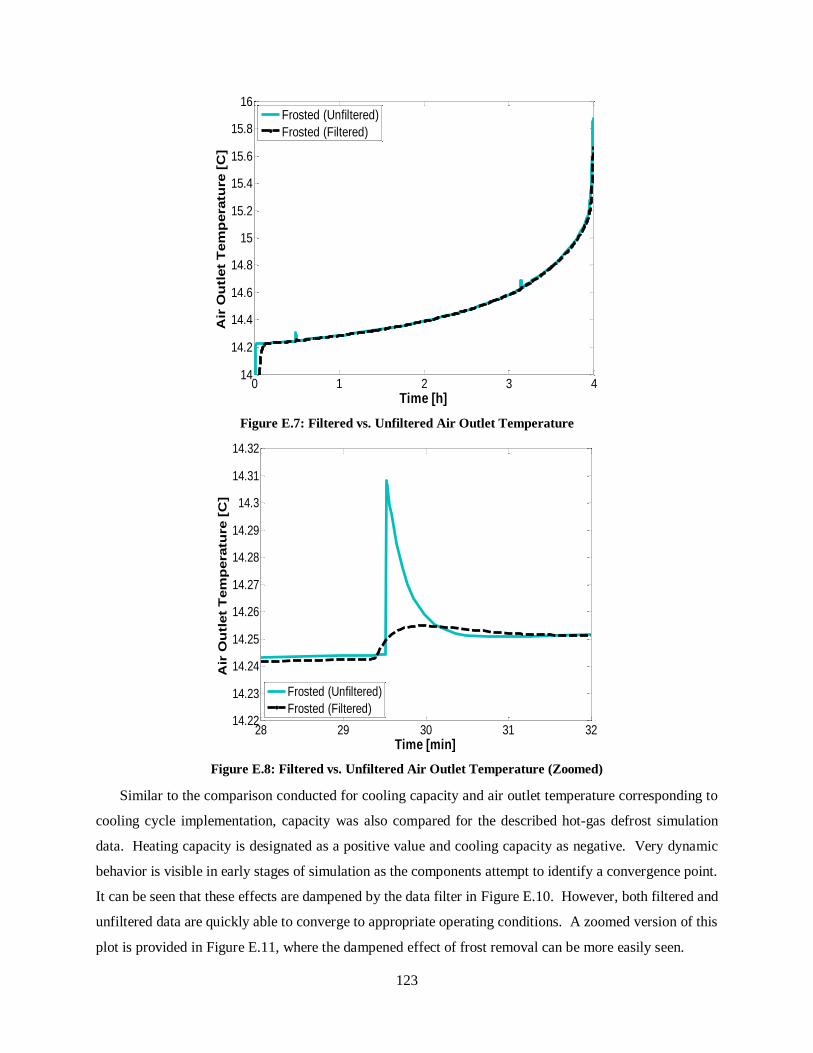
123

Figure E.7: Filtered vs. Unfiltered Air Outlet Temperature

Figure E.8: Filtered vs. Unfiltered Air Outlet Temperature (Zoomed)

Similar to the comparison conducted for cooling capacity and air outlet temperature corresponding to

cooling cycle implementation, capacity was also compared for the described hot-gas defrost simulation

data. Heating capacity is designated as a positive value and cooling capacity as negative. Very dynamic

behavior is visible in early stages of simulation as the components attempt to identify a convergence point.

It can be seen that these effects are dampened by the data filter in Figure E.10. However, both filtered and

unfiltered data are quickly able to converge to appropriate operating conditions. A zoomed version of this

plot is provided in Figure E.11, where the dampened effect of frost removal can be more easily seen.

0 1 2 3 414

14.2

14.4

14.6

14.8

15

15.2

15.4

15.6

15.8

16

Time [h]

Air

Ou

tlet

Tem

pera

ture

[C

]

Frosted (Unfiltered)

Frosted (Filtered)

28 29 30 31 3214.22

14.23

14.24

14.25

14.26

14.27

14.28

14.29

14.3

14.31

14.32

Time [min]

Air

Ou

tlet

Tem

pera

ture

[C

]

Frosted (Unfiltered)

Frosted (Filtered)

124

Figure E.9: Defrost Cycle Heating Capacity vs. Time (Unfiltered)

Figure E.10: Filtered vs. Unfiltered Defrost Cycle Heating Capacity

0 3 6 9 12 15 18 21 24 27 300

1

2

3

4

5

6

Time [min]

Heati

ng

Cap

acit

y [

W]

Baseline

Finned Unfrosted

Frosted (Unfiltered)

0 3 6 9 12 15 18 21 24 27 30-45

-40

-35

-30

-25

-20

-15

-10

-5

0

5

Time [min]

Cap

acit

y [

W]

Frosted (Unfiltered)

Frosted (Filtered)

125

Figure E.11: Filtered vs. Unfiltered Defrost Cycle Heating Capacity (Zoomed)

0 3 6 9 12 15 18 21 24 27 300

1

2

3

4

5

6

7

Time [min]

Heati

ng

Cap

acit

y [

W]

Frosted (Unfiltered)

Frosted (Filtered)

126

List of References

[1] Alebrahim, A. M., and S. A. Sherif. “Electric Defrosting Analysis of a Finned-Tube Evaporator Coil

Using the Enthalpy Method.” 216 (2002): 655–673. Web.

[2] Ali, D A, R R Crawford, and Air Conditioning. “The Effects of Frost Formation on the Performance

of Domestic Refrigerator-Freezer Finned-Tube Evaporator Coils.” (1992). Web.

[3] Aljuwayhel, N.F. et al. “Experimental Investigation of the Performance of Industrial Evaporator Coils

Operating under Frosting Conditions.” International Journal of Refrigeration 31.1 (2008): 98–106.

Web. 17 Sept. 2014.

[4] Chua, K.J., S.K. Chou, and W.M. Yang. “Advances in Heat Pump Systems: A Review.” Applied

Energy 87.12 (2010): 3611–3624. Web. 6 Aug. 2013.

[5] Cui, J. et al. “A New Model for Predicting Performance of Fin-and-Tube Heat Exchanger under Frost

Condition.” International Journal of Heat and Fluid Flow 32.1 (2011): 249–260. Web. 28 Oct. 2014.

[6] Cui, J. et al. “A New Time- and Space-Dependent Model for Predicting Frost Formation.” Applied

Thermal Engineering 31.4 (2011): 447–457. Web. 13 Mar. 2015.

[7] Datta, D, S. Tassou, and D. Marriott. “Experimental Investigations into Frost Formation on Display

Cabinet Evaporators in Order to Implement Defrost on Demand.” International Refrigeration and Air

Conditioning Conference, 1998. Web.

[8] Dong, Jiankai et al. “An Experimental Study on Defrosting Heat Supplies and Energy Consumptions

during a Reverse Cycle Defrost Operation for an Air Source Heat Pump.” Applied Thermal

Engineering 37 (2012): 380–387. Web. 9 Feb. 2015.

[9] Dopazo, J. Alberto et al. “Modelling and Experimental Validation of the Hot-Gas Defrost Process of

an Air-Cooled Evaporator.” International Journal of Refrigeration 33.4 (2010): 829–839. Web. 12

Sept. 2013.

[10] Fasl, J. “Modeling and Control of Hybrid Vapor Compression Cycles.” University of Illinois at

Urbana-Champaign, 2013. Print.

[11] Fricke, Brian A. Ph.D., and Vishal Sharma. Demand Defrost Strategies in Supermarket Refrigeration

Systems Prepared by : Oak Ridge, TN. 2011. Web.

127

[12] Getu, H.M., and P.K. Bansal. “New Frost Property Correlations for a Flat-Finned-Tube Heat

Exchanger.” International Journal of Thermal Sciences 50.4 (2011): 544–557. Web. 4 Feb. 2015.

[13] Gogos, G. Computational Heat Transfer and Fluid Flow [Course Notes]. MECH 431 (Spring 2013).

Department of Mechanical Engineering. University of Nebraska.

[14] Heating and Cooling. US Department of Energy. http://energy.gov/public-services/homes/heating-

cooling.

[15] Hermes, Christian J.L. et al. “A Study of Frost Growth and Densification on Flat Surfaces.”

Experimental Thermal and Fluid Science 33.2 (2009): 371–379. Web. 19 Sept. 2013.

[16] Hoffenbecker, Nathan. “Investigation of Alternative Defrost Strategies.” University of Wisconsin-

Madison, 2004. Print.

[17] Hoffenbecker, N., S.A. Klein, and D.T. Reindl. “Hot Gas Defrost Model Development and

Validation.” International Journal of Refrigeration 28.4 (2005): 605–615. Web.

[18] Incropera, Frank P., David P. DeWitt, Theodore L. Bergman, and Adrienne S. Lavine. Fundamentals

of Heat and Mass Transfer. Seventh ed. John Wiley & Sons, 2011. Print.

[19] Iragorry, Jose, Yong-xin Tao, and Shaobo Jia. “A Critical Review of Properties and Models for Frost

Formation Analysis.” 10.4 (2004): n. pag. Web.

[20] Kondepudi, Sekhar N, and Dennis L O Neal. “Performance of Finned-Tube Heat Exchangers under

Frosting Conditions : I Simulation Model Performance” 1.3 (1993): 175–180. Web.

[21] Kondepudi, Sekhar N, and Dennis L O Neal. “Performance of Finned-Tube Heat Exchangers under

Frosting Conditions : II Comparison of Experimental Data with Model Performance”. 4.3

(1993).Web.

[22] Lee, Y B, and S T Ro. “An Experimental Study of Formation on a Horizontal Cylinder Under Cross

Flow.” International Journal of Refrigeration 24 (2001): 468–474. Web.

[23] Lee, T. H.; Lee, K. S.; and Kim, W. S., "The Effects of Frost Formation in a Flat Plate Finned-Tube

Heat Exchanger" (1996). International Refrigeration and Air Conditioning Conference. Paper 325.

http://docs.lib.purdue.edu/iracc/325

[24] Liu, Zhiqiang, Guangfa Tang, and Fuyun Zhao. “Dynamic Simulation of Air-Source Heat Pump

during Hot-Gas Defrost.” Applied Thermal Engineering 23.6 (2003): 675–685. Web. 12 Sept. 2013.

[25] Mills, A.F. Heat Transfer. 2nd ed. Upper Saddle River, NJ: Prentice Hall, 1999. Print.

[26] Mohs, William. “Heat and Mass Transfer During the Melting Process of a Porous Frost Layer on a

Vertical Surface.” University of Minnesota, 2013. Print.

[27] Moran, Michael J., Howard N. Shapiro, Daisie D. Boettner, and Margaret B. Bailey. Fundamentals

of Engineering Thermodynamics. 7th ed. New York: Wiley, 2011. Print.

128

[28] Muehlbauer, Jan. “Investigation of Performance Degradation of Evaporator for Low Temperature

Refrigeration.” University of Maryland, College Park, 2006. Print.

[29] Nelson, Bruce I., P.E. (Colmac Coil Manufacturing, Inc.). “Optimizing Hot Gas Defrost.” 2011. Web.

[30] Patankar, Suhas V. Numerical Heat Transfer and Fluid Flow. Washington: Hemisphere Pub., 1980.

Print.

[31] Reindl, Douglas T., Ph.D, P.E and Jekel, Todd B, and Ph.D. “Defrosting Industrial Refrigeration

Evaporators.” ASHRA Journal August (2009): 30–40. Web.

[32] Reindl, Douglas T., Ph.D, P.E and Jekel, Todd B, and Ph.D. “On Air-Cooling Evaporators.” ASHRAE

Journal February (2009): 27–33. Web.

[33] Sommers, a. D., and a. M. Jacobi. “An Exact Solution to Steady Heat Conduction in a Two-

Dimensional Annulus on a One-Dimensional Fin: Application to Frosted Heat Exchangers with

Round Tubes.” Journal of Heat Transfer 128.4 (2006): 397. Web. 6 Feb. 2015.

[34] Tso, C.P., Y.C. Cheng, and a.C.K. Lai. “An Improved Model for Predicting Performance of Finned

Tube Heat Exchanger under Frosting Condition, with Frost Thickness Variation along Fin.” Applied

Thermal Engineering 26.1 (2006): 111–120. Web. 25 Jan. 2015.

[35] Tu, Ping et al. “Fin Efficiency of an Annular Fin Composed of a Substrate Metallic Fin and a Coating

Layer.” Journal of Heat Transfer 128.8 (2006): 851. Web. 22 Jan. 2015.

[36] Wang, W. et al. “A Generalized Simple Model for Predicting Frost Growth on Cold Flat Plate.”

International Journal of Refrigeration 35.2 (2012): 475–486. Web. 11 Sept. 2013.

[37] Xia, Y.and A.M. Jacobi. “An Exact Solution to Steady Heat Conduction in a Two-Dimensional Slab

on a One-Dimensional Fin: Application to Frosted Heat Exchangers.” International Journal of Heat

and Mass Transfer 47.14-16 (2004): 3317–3326. Web. 6 Feb. 2015.

[38] Xia, Y. et al. “Frost, Defrost, and Refrost and Its Impact on the Air-Side Thermal-Hydraulic

Performance of Louvered-Fin, Flat-Tube Heat Exchangers.” International Journal of Refrigeration

29.7 (2006): 1066–1079. Web. 10 Feb. 2015.

[39] Yan, Wei-Mon et al. “Performance of Finned Tube Heat Exchangers Operating under Frosting

Conditions.” International Journal of Heat and Mass Transfer 46.5 (2003): 871–877. Web.

[40] Yang, Dong-Keun, Kwan-Soo Lee, and Simon Song. “Modeling for Predicting Frosting Behavior of

a Fin–tube Heat Exchanger.” International Journal of Heat and Mass Transfer 49.7-8 (2006): 1472–

1479. Web. 25 Jan. 2015.