DYNAMIC MODELING AND CONTROL OF A HYBRID FIN …etd.lib.metu.edu.tr/upload/12618256/index.pdf ·...
154
DYNAMIC MODELING AND CONTROL OF A HYBRID FIN ACTUATION SYSTEM FOR AN AIR-TO-AIR MISSILE A THESIS SUBMITTED TO THE GRADUATE SCHOOL OF NATURAL AND APPLIED SCIENCES OF MIDDLE EAST TECHNICAL UNIVERSITY BY TAYFUN ÇELİK IN PARTIAL FULFILLMENT OF THE REQUIREMENTS FOR THE DEGREE OF MASTER OF SCIENCE IN MECHANICAL ENGINEERING DECEMBER 2014
Transcript of DYNAMIC MODELING AND CONTROL OF A HYBRID FIN …etd.lib.metu.edu.tr/upload/12618256/index.pdf ·...

DYNAMIC MODELING AND CONTROL OF A HYBRID FIN ACTUATION SYSTEM FOR AN AIR-TO-AIR MISSILE
A THESIS SUBMITTED TO
THE GRADUATE SCHOOL OF NATURAL AND APPLIED SCIENCES OF
MIDDLE EAST TECHNICAL UNIVERSITY
BY
TAYFUN ÇELİK
IN PARTIAL FULFILLMENT OF THE REQUIREMENTS FOR
THE DEGREE OF MASTER OF SCIENCE IN
MECHANICAL ENGINEERING
DECEMBER 2014


Approval of the thesis:
DYNAMIC MODELING AND CONTROL OF A HYBRID FIN ACTUATION SYSTEM FOR AN AIR-TO-AIR MISSILE
submitted by TAYFUN ÇELİK in partial fulfillment of the requirements for the degree of Master of Science in Mechanical Engineering Department, Middle East Technical University by,
Prof. Dr. Gülbin Dural Ünver __________________ Dean, Graduate School of Natural and Applied Sciences Prof. Dr. R. Tuna Balkan __________________ Head of Department, Mechanical Engineering Assoc. Prof. Dr. Ender Ciğeroğlu __________________ Supervisor, Mechanical Engineering Dept., METU Assist. Prof. Dr. Yiğit Yazıcıoğlu __________________ Co-Supervisor, Mechanical Engineering Dept., METU Examining Committee Members: Prof. Dr. Reşit Soylu __________________ Mechanical Engineering Dept., METU Assoc. Prof. Dr. Ender Ciğeroğlu __________________ Mechanical Engineering Dept., METU Assist. Prof. Dr. Kıvanç Azgın __________________ Mechanical Engineering Dept., METU Assist. Prof. Dr. Yiğit Yazıcıoğlu __________________ Mechanical Engineering Dept., METU Dr. Bülent Özkan __________________ Mechatronics Division, TÜBİTAK SAGE
Date : __________________

iv
I hereby declare that all information in this document has been obtained and presented in accordance with academic rules and ethical conduct. I also declare that, as required by these rules and conduct, I have fully cited and referenced all material and results that are not original to this work.
Name, Last name : Tayfun ÇELİK
Signature :
v
ABSTRACT
DYNAMIC MODELING AND CONTROL OF A HYBRID FIN ACTUATION
SYSTEM FOR AN AIR-TO-AIR MISSILE
Çelik, Tayfun
M.S., Department of Mechanical Engineering
Supervisor : Assoc. Prof. Dr. Ender Ciğeroğlu
Co-Supervisor : Assist. Prof. Dr. Yiğit Yazıcıoğlu
December 2014, 136 pages
Air-to-air missiles require high maneuverability. In order to obtain high
maneuverability, hybrid fin actuation systems are used. In this study, a hybrid fin
actuation system which is composed of aerodynamic control surfaces and thrust
vector control is designed. Both aerodynamic and thrust vector control types are
explained and the most suitable pair is determined for air-to-air missile. Then, the
designed system is physically constructed and system identification procedure is
performed. After that three different controllers PID, H∞ and 2-DOF H∞ controllers
are designed and tested on both on the real system and simulation environment.
Finally, all the results are compared with the cascaded H∞ controller.
Keywords: Fin actuation systems, jet vane, H∞ robust control, system identification,
cascaded systems
vi
ÖZ
HAVADAN HAVAYA FÜZELER İÇİN MELEZ KANATÇIK TAHRİK
TASARIMI VE MODELLENMESİ
Çelik, Tayfun
Yüksek Lisans, Makina Mühendisliği Bölümü
Tez Yöneticisi : Doç. Dr. Ender Ciğeroğlu
Ortak Tez Yöneticisi : Yrd. Doç. Dr. Yiğit Yazıcıoğlu
Aralık 2014, 136 sayfa
Havadan-havaya füzeler yüksek manevra kabiliyeti gerektirmektedir. Bu yüksek
manevra kabiliyetini yakalamak için melez kanatçık tahrik sistemleri
kullanılmaktadır. Bu çalışmada aerodinamik yüzeylerin kontrolü ve itki vektör
kontrolü sistemi içeren melez bir kanatçık tahrik sistemi tasarlanmıştır. Hem
aerodinamik hem de itki vektör kontrol yöntemleri hakkında bilgi verilmiştir. Bu
sistemlerden hava-hava füzesi için en uygun ikiliye karar verilerek sistemin üretimi
gerçekleştirilmiştir. Bu sistem için PID, H∞ ve ikinci derece H∞ kontrolcüler
tasarlanmıştır. Bu kontrolcüler hem benzetim ortamında hem de sistem üzerinde
denemiştir. Son olarak sistem için çift döngülü, her iki döngüsünde de H∞ kontrolcü
olan kontrolcüyle test edilmiş ve elde edilen sonuçlar diğer kontrolcülerle elde edilen
sonuçlarla karşılaştırılmıştır.
Anahtar kelimeler: Kanatçık tahrik sistemleri, jet vanası, H∞ gürbüz kontrol, sistem
tanımlama, çift döngülü sistem

vii
To My Parents
and
My Love Pınar Çelik

viii
ACKNOWLEDGEMENTS
I would like to send my thanks to my supervisor Assoc. Prof. Dr. Ender
CİĞEROĞLU. During preparation of my thesis, my supervisor gave me very special
support by his helpful criticism, guidance and patience. I would also like to thank to
my co-supervisor Assist. Prof. Dr. Yiğit YAZICIOĞLU due to his contribution.
I want to express my appreciation to my head of division Dr. Bülent ÖZKAN. His
encouragements and technical support during progress of the thesis are very
valuable. I also specially want to thank to my colleague Berkay BAYKARA for his
endless help and patience. My colleague Göktuğ Gencehan ARTAN's
encouragements and motivation for this work are delicately appreciated.
I am very grateful to support of TÜBİTAK BİDEB and facilities of TÜBİTAK
SAGE in the application of experimental studies of my thesis.
I want to send my thanks to all members of family. They give me endless support
and patience throughout my life.
Finally, I am very thankful to my wife Pınar ÇELİK. During progress and
preparation of my thesis, my love gave me all motivation and energy for finishing
this work.
ix
TABLE OF CONTENTS
ABSTRACT ................................................................................................................. v
ÖZ ............................................................................................................................... vi
ACKNOWLEDGEMENTS ...................................................................................... viii
TABLE OF CONTENTS ............................................................................................ ix
LIST OF TABLES .................................................................................................... xiii
LIST OF FIGURES .................................................................................................. xiv
CHAPTERS ................................................................................................................. 1
1. INTRODUCTION ................................................................................................... 1
1.1 Aim of the Study ............................................................................................ 1
1.2 Scope of the Thesis ........................................................................................ 1
1.3 Background and Basic Concepts ................................................................... 2
1.3.1 A General Information about Air-to-Air Missile (AAM) ....................... 2
1.3.2 Control Actuation System (CAS) ........................................................... 3
1.4 Types of Control Systems .............................................................................. 4
1.4.1 Aerodynamic Control ............................................................................. 4
1.4.1.1 Wing Control .................................................................................. 5
1.4.1.2 Canard Control ................................................................................ 5
1.4.1.3 Tail Control ..................................................................................... 6
1.4.2 Control Surface Arrangement ................................................................. 6
1.4.2.1 Monowing ....................................................................................... 7
1.4.2.2 Triform ............................................................................................ 7
1.4.2.3 Cruciform ........................................................................................ 7
1.4.3 Thrust Vector Control (TVC) ................................................................. 7
1.4.3.1 Movable Nozzle Systems (MNS) ................................................... 9
1.4.3.1.1 Flexible Joint Method ........................................................... 10
1.4.3.1.2 Gimbaled Nozzle Method .................................................... 11
1.4.3.1.3 Ball in Socket Type Nozzle .................................................. 11
x
1.4.3.1.4 Hinged Nozzle Method ......................................................... 11
1.4.3.2 Fixed Nozzle Systems ................................................................... 12
1.4.3.2.1 Secondary Injection Thrust Vector Control (SITVC) .......... 12
1.4.3.2.1.1 Liquid Injection ............................................................. 13
1.4.3.2.1.2 Gas Injection .................................................................. 13
1.4.3.2.2 Mechanical Deflector ........................................................... 14
1.4.3.2.2.1 Jet Vane ......................................................................... 14
1.4.3.2.2.2 Jet Tab ........................................................................... 16
1.4.3.2.2.3 Jetevator ......................................................................... 16
1.4.3.3 Reaction Control ........................................................................... 17
1.4.3.3.1 Reaction Jet .......................................................................... 17
1.5 Basic Concepts of Hybrid Fin Actuation Systems ....................................... 18
1.6 Review of the Literature on H∞ Control ...................................................... 19
1.6.1 Historical Background .......................................................................... 19
1.7 Theoretical Background of Robust Control ................................................. 19
1.7.1 Reasons for Robust Control .................................................................. 19
1.7.2 Problem Statement ................................................................................ 20
1.7.3 Norms of Systems ................................................................................. 21
1.7.4 Linear Fractional Transformation (LFT) .............................................. 22
1.7.5 Sensitivity, Robustness and Feedback Structure................................... 23
1.7.6 Plant Uncertainty, Stability and Performance ....................................... 24
1.7.7 Solution to H∞ Problem ......................................................................... 29
1.8 Literature Review of the Electro-Mechanical Actuator Control .................. 31
2. SYSTEM MODELING AND IDENTIFICATION ............................................... 33
2.1 Modeling of the System ............................................................................... 33
2.2 Mathematical Models of System .................................................................. 34
2.2.1 Motion Transmission Mechanism ......................................................... 34
2.2.2 Sensors .................................................................................................. 37
2.2.3 DC Motor .............................................................................................. 38
2.2.4 External Loads and Disturbances .......................................................... 42

xi
2.3 System Identification ................................................................................... 42
3. CONTROLLER DESIGN ...................................................................................... 55
3.1 Requirements for the Closed Loop System ................................................. 55
3.2 PID Controller Synthesis ............................................................................. 56
3.3 Synthesis of Robust Controllers ................................................................... 64
3.3.1 Selection of Weighting Functions ......................................................... 70
3.3.1.1 Model Uncertainty ........................................................................ 74
3.3.1.2 Weighting Function for Reference Signal refW ............................ 77
3.3.1.3 Weighting Function for Aerodynamic Loads hingeW .................... 77
3.3.1.4 Cost Function for Controller Output uW ...................................... 78
3.3.1.5 Ideal Close Loop System, idealW ................................................... 79
3.3.1.6 Cost Function for Performance Requirements, perfW ................... 79
3.3.1.7 Weighting Function for Sensor Noise nW .................................... 80
3.3.2 H∞ Controller Synthesis ........................................................................ 80
3.3.3 2-DOF H∞ Controller Synthesis ............................................................ 84
3.3.4 Cascaded H∞ Controller Synthesis ........................................................ 88
3.3.4.1 H∞ Speed Controller ..................................................................... 89
3.3.4.2 H∞ Position Controller .................................................................. 92
4. COMPUTER SIMULATIONS AND EXPERIMENTS ........................................ 95
4.1 Simulation Results ....................................................................................... 95
4.2 Experimental Results ................................................................................... 98
4.2.1 Experimental Bandwidth of the System ............................................. 102
5. DISCUSSION AND CONCLUSION .................................................................. 105
5.1 Summary and Comments on the Results ................................................... 105
5.2 Future Works ............................................................................................. 106
REFERENCES ......................................................................................................... 109
APPENDICES ......................................................................................................... 117
A.1. Air-to-Air Missiles ..................................................................................... 117
A.2. System Identification Input-Outputs in Time Domain .............................. 122

xii
A.3. Frequency Spectrum of Input Signals ........................................................ 125
A.4. Generalized Plant Matrices ........................................................................ 128
A.5. Weightings Functions of Cascade H∞ Controller ....................................... 136

xiii
LIST OF TABLES
TABLES
Table 1. Parameters of mechanism ............................................................................ 37
Table 2. Process model parameter estimation and percentage of the fittings ........... 50
Table 3. Minimum performance requirements of the system .................................... 56
Table 4. Ziegler Nichols tuning formula based on step response .............................. 62
Table 5. Ziegler Nichols tuning formula based on frequency response ..................... 63
Table 6. Comparison of the robust controllers ......................................................... 103
Table 7. Air-to-Air missiles [4] ................................................................................ 117

xiv
LIST OF FIGURES
FIGURES
Figure 1. Auto pilot of the missile [5] .......................................................................... 4
Figure 2. Missile motions [3] ....................................................................................... 4
Figure 3. Air Vane Control Techniques [6] ................................................................. 5
Figure 4. Arrangements of missile fins ........................................................................ 6
Figure 5."+" and "x" cruciform arrangement ............................................................... 7
Figure 6. Working principles of TVC [8] .................................................................... 8
Figure 7. Thrust vector control systems ....................................................................... 8
Figure 8. Flight maneuvers of four-fixed position thrust chambers [3] ....................... 9
Figure 9. Schematic of flexible nozzle [11] ............................................................... 10
Figure 10. Schematic of ball & socket nozzle [11] .................................................... 11
Figure 11. Schematic of secondary injection method [14] ......................................... 13
Figure 12. Liquid injection TVC system [9] .............................................................. 13
Figure 13. Gas injection TVC system [9] .................................................................. 14
Figure 14. Jet vanes of German V-2 Rockets [15] ..................................................... 15
Figure 15. Jet tab TVC system [23] ........................................................................... 16
Figure 16. Jetevator TVC system adapted from [23] ................................................. 17
Figure 17. Projectile reaction jet control system adapted from [27] .......................... 18
Figure 18. Standard LTI feedback block diagram ...................................................... 20
Figure 19. System G(s) operating on signal w(s) ....................................................... 21
Figure 20. Upper fractional transformation ................................................................ 23
Figure 21. Typical feedback loop with disturbances .................................................. 23
Figure 22. Multiplicative uncertainty ......................................................................... 26
Figure 23. Additive uncertainty ................................................................................. 26
Figure 24. Feedback system with a multiplicative uncertainty .................................. 27
Figure 25. Nyquist plot of Lp for robust stability [39] ............................................... 27

xv
Figure 26. Nyquist plot of nominal performance condition [39] ............................... 28
Figure 27. Backside view of AAM and coordinate frame of a fin ............................. 34
Figure 28. Schematic diagram of the FAS ................................................................. 35
Figure 29. Transmission ratio of the system .............................................................. 37
Figure 30. Equivalent circuit of the DC motor .......................................................... 39
Figure 31. Block diagram of the DC motor between voltage and motor position ..... 40
Figure 32. A dynamic system with input u(t) and output y(t) .................................... 42
Figure 33. A PRBS input signal used in system identification .................................. 45
Figure 34. A BLWN input signal used in system identification ................................ 46
Figure 35. Frequency spectrum of the input signals .................................................. 46
Figure 36. System identification toolbox GUI ........................................................... 48
Figure 37. Comparison of estimation results with outputs ........................................ 49
Figure 38. Frequency response of experimental outputs ........................................... 51
Figure 39. Fitted transfer functions ............................................................................ 51
Figure 40. Output of the DataB2 ................................................................................ 52
Figure 41. Output of the DataP3 ................................................................................ 52
Figure 42. Output of the DataB4 ................................................................................ 53
Figure 43. Obtained eqB values ................................................................................. 53
Figure 44. Fin actuation system block diagram for PID controller ........................... 57
Figure 45. Discrete time PID controller ..................................................................... 59
Figure 46. Reference signal tracking of the PID controllers ...................................... 59
Figure 47. Magnification of step response at t=1s in Figure 46 ................................ 60
Figure 48. Current commands of PID controllers ...................................................... 60
Figure 49. The main block diagram used in simulations ........................................... 61
Figure 50. Subsystem of the main block diagram ...................................................... 61
Figure 51. Response of the FOPDT model [33] ........................................................ 62
Figure 52. Step response of the system to determine Kp ........................................... 63
Figure 53. Step response comparison of Z-N Tuned PID .......................................... 64
Figure 54. Block diagram for H∞ robust controller .................................................... 66
Figure 55. Block diagram for 2-DOF H∞ robust controller ....................................... 67
xvi
Figure 56. Block diagram for cascade H∞ robust controller ...................................... 68
Figure 57. Block diagram for inner loop velocity H∞ robust controller ..................... 69
Figure 58. Generalized plant for controller synthesis ................................................ 70
Figure 59. Typical sensitivity function [38] ............................................................... 71
Figure 60. Typical complementary function [38] ...................................................... 71
Figure 61. Performance weight function .................................................................... 72
Figure 62. Control signal weight function ................................................................. 73
Figure 63. Bode plot of uncertain system .................................................................. 74
Figure 64. Bode plot of uncertain system with known tK and eqJ .......................... 74
Figure 65. Representation of plant uncertainties term by term .................................. 75
Figure 66. Representation of whole plant uncertainty ............................................... 75
Figure 67. Approximation of uncertain transfer function by multiplicative uncertainty
.................................................................................................................................... 76
Figure 68. Magnitude plot of the reference weight function, refW ............................. 77
Figure 69. Magnitude plot of the aerodynamic loads, hingeW ...................................... 78
Figure 70. Magnitude plot of the controller output loads, 1 / uW ............................... 78
Figure 71. Bode plot of the ideal closed loop system ................................................ 79
Figure 72. Magnitude plot of the controller output, 1 / perfW ..................................... 80
Figure 73. Step response of the uncertain system ...................................................... 81
Figure 74. Singular value plot of sensitivity function ................................................ 82
Figure 75. Singular value plot of complementary sensitivity function ...................... 82
Figure 76. Singular value plot of open loop gain and sensitivity function of uncertain
system ......................................................................................................................... 83
Figure 77. Simulation and experimental results of H∞ controller .............................. 83
Figure 78. Magnification of step response at t=1 s in Figure 76 ................................ 84
Figure 79. Current consumption of H∞ Controller ..................................................... 84
Figure 80. Step response of the uncertain system (2-DOF H∞) ................................. 85
Figure 81. Singular value plot of sensitivity function (2-DOF H∞) ........................... 86
Figure 82. Closed loop Bode diagram of 2-DOF H∞ controlled system .................... 86
xvii
Figure 83. Open loop gain and sensitivity function of uncertain system (2-DOF H∞)
.................................................................................................................................... 87
Figure 84. Simulation and experimental results of 2-DOF H∞ Controller ................. 87
Figure 85. Magnification of step response at t=1 s in Figure 84 ............................... 88
Figure 86. Current consumption of 2-DOF H∞ controller ......................................... 88
Figure 87. Step response of the uncertain system (H∞ speed) ................................... 89
Figure 88. Open loop gain and sensitivity function of the system (H∞ speed) .......... 90
Figure 89. Closed loop Bode diagram of H∞ speed controlled system ...................... 90
Figure 90. Simulation and experimental results of H∞ speed controlled system ....... 91
Figure 91. Magnification of step response at t=1 s in Figure 90 ............................... 91
Figure 92. Current consumption of H∞ speed controller ............................................ 92
Figure 93. Closed loop Bode diagram of cascaded H∞ controlled system ................. 92
Figure 94. Simulation and experimental results of cascaded H∞ controller............... 93
Figure 95. Magnification of step response at t=1 s in Figure 94 ............................... 93
Figure 96. Current consumption of cascaded H∞ controller ...................................... 94
Figure 97. Sensitivity functions of the closed loop systems with different controller
.................................................................................................................................... 95
Figure 98. Singular value plot of the loop transfer functions with different controllers
.................................................................................................................................... 96
Figure 99. Step response of controllers ...................................................................... 97
Figure 100. Bode diagrams of the closed loop system .............................................. 97
Figure 101. Responses of the closed loop systems .................................................... 98
Figure 102. Detailed view of the step responses at t=1 s in Figure 101 .................... 98
Figure 103. Controller output of the system .............................................................. 99
Figure 104. Response of the system to 1 Hz signal ................................................... 99
Figure 105. Controller output of the system to 1 Hz signal ..................................... 100
Figure 106. Reference tracking of the system under variable disturbance .............. 101
Figure 107. Controller output of the system under variable disturbance ................. 101
Figure 108. Response of H∞ cascaded controlled system to chirp signal ................ 102
Figure 109. Input and output signal set used in identification ................................. 124

xviii
Figure 110. Frequency content of input signals ....................................................... 127
1
CHAPTER 1
INTRODUCTION
1.1 Aim of the Study
Air-to-air missiles are very agile munitions that are designed to hit aerial targets.
Most of them are equipped with both thrust vector control (TVC) and aerodynamic
control surfaces.
In this study, the practicability of the TVC and aerodynamic control surfaces are
examined and the most proper pair is chosen and constructed. The challenges of this
system is that, it should be compact and modular. The designed system is both
affected by aerodynamic forces and exhaust gas of rocket motor so that during the
flight of the missile, fin actuation system must be stable and give satisfactory
performance required by the physical system and concept of operation. In this thesis,
electromechanical system is designed that contains a motor, an encoder, a gear pair
and a four link mechanism. The system has some nonlinearities due to its physical
nature such as gear backlash. In the light of these facts, the system is simulated and
tested by robust controllers.
In this thesis, cascaded H∞ norm-based control approach is applied to the fin
actuation system and this controller is compared in terms of stability and
performance to H∞, 2-DOF H∞ and PID controllers.
1.2 Scope of the Thesis
In Chapter 1, the general information about the aerodynamic control and TVC
control systems are given such that the idea behind the system is well defined. Then,

2
the theory of the robust control is presented in summary. At the end of this chapter,
similar works that are done for control/fin actuation system are given.
In Chapter 2, the physical system is interpreted in detail. The subcomponents of the
system are interpreted and their mathematical models are derived in this part. Then
the total system is identified and made ready to implement the controller which is
synthesized according to the identified plant model.
In Chapter 3, PID, 1-DOF H∞, 2-DOF H∞ and cascaded H∞ of controllers are
designed and exhibited. All of them are simulated and tested with physical system.
All the data obtained are presented in this section.
In Chapter 4, computer simulations and test results of the controllers are compared
and represented in this section.
And finally in Chapter 5, the results are discussed and summarized. The related
future works are also proposed in this chapter.
1.3 Background and Basic Concepts
1.3.1 A General Information about Air-to-Air Missile (AAM)
An air-to-air missile is launched from an aerial platform to destroy an opposing one.
In general manner, AAMs are used to protect air space, air vehicles and other aerial
platforms from hostile air forces. AAMs are broadly divided in two groups which are
short range "within visual range" and medium or long range "beyond visual range"
missiles. Short range missiles are launched to destroy the enemy aircraft when the
hostile platform is close enough and there is no chance to fire medium or long range
missile. Short range AAMs are much more agile than long range missiles because of
the limited range to maneuver; therefore, some of them have thrust vector control
unit to develop agility. On the contrary, medium range missiles are optimized to
enhance performance and weight while long range missiles are designed to increase
speed and range. They are also equipped with a radar seeker unit. Both of them have
some advantages over another but the current developments show that shooting down
an enemy from a distance is a new trend. For this reason, MBDA, a multi-national
missile corporation was formed by Matra Missile, BAE Dynamics and Alenia
Marconi Systems that currently develops Meteor ramjet engine for a long range

3
missile and several nations try to develop their long range missiles [1].
1.3.2 Control Actuation System (CAS)
Control actuation system (CAS) is an important part of a missile which steers the
missile according to the commands coming from guidance system which means that
CAS converts an electrical input command to an appropriate output shaft angle as
seen in Figure 1 [2]. CAS is composed of electronic cards 'driver etc.', power sources
'thermal battery' and fin actuation system (FAS). Typically, there are three major
types of control systems which are aerodynamic control, thrust vector control and
reaction control. In a missile, they can be used individually or together. Especially
for AAM, maneuverability is severe when it is compared to other missiles such as
cruise, ballistic etc. Therefore, in order to follow desired path both of these
techniques can be applied. In the sense of AAM, the main idea of using together is
to enhance the desired maneuverability.
Missile configuration design decides the FAS space, weight limitations, types of
control elements and power requirements while the missile stabilization and
guidance loop determines the FAS requirements. According to FAS mechanical
design, FASs are classified as electro-hydraulic, electromechanical or electro-
pneumatic. Hydraulic type actuators are used where large forces are required. For
example, Tomahawk cruise missile uses hydraulic actuators while AIM 9L/M/N
have pneumatic actuators because forces acting on aerodynamic surfaces are
imperatively small enough to control using pneumatic actuators [3]. The difference
comes from , power requirement, package of system, cost, reliability, repeatability,
manufacturability, and controllability. But today's AAMs are usually equipped with
electromechanical FAS [4].
4
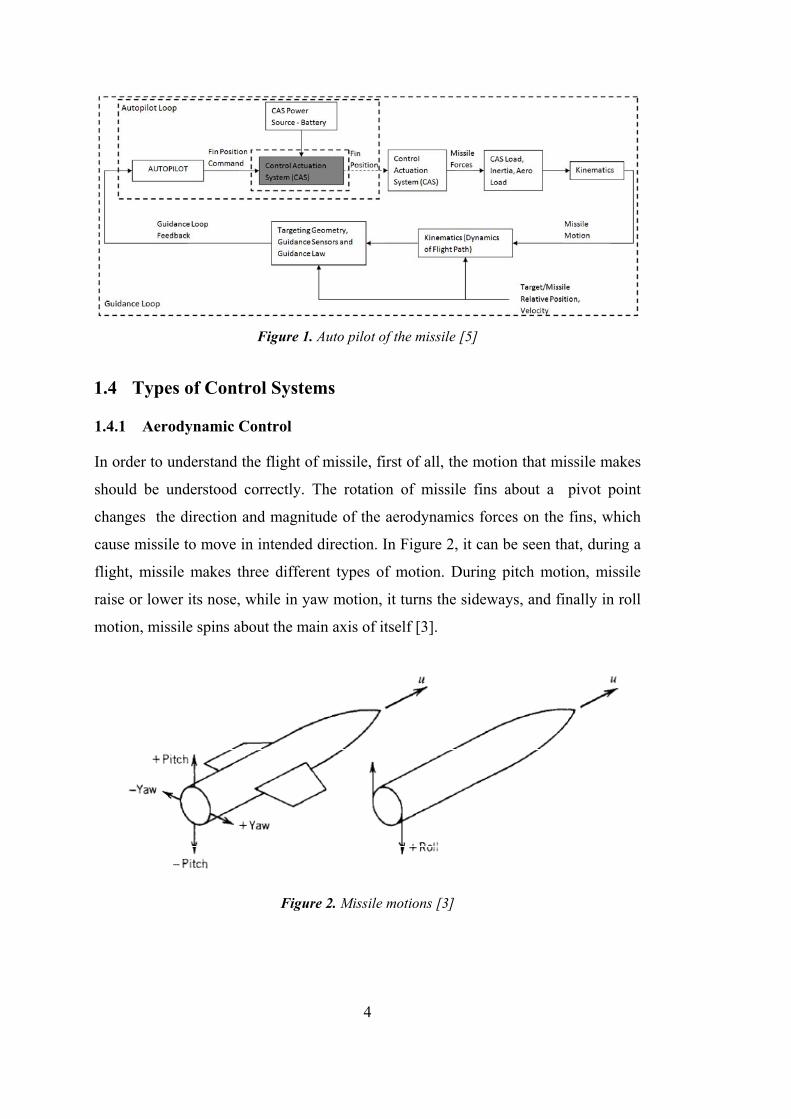
Figure 1. Auto pilot of the missile [5]
1.4 Types of Control Systems
1.4.1 Aerodynamic Control
In order to understand the flight of missile, first of all, the motion that missile makes
should be understood correctly. The rotation of missile fins about a pivot point
changes the direction and magnitude of the aerodynamics forces on the fins, which
cause missile to move in intended direction. In Figure 2, it can be seen that, during a
flight, missile makes three different types of motion. During pitch motion, missile
raise or lower its nose, while in yaw motion, it turns the sideways, and finally in roll
motion, missile spins about the main axis of itself [3].
Figure 2. Missile motions [3]
5
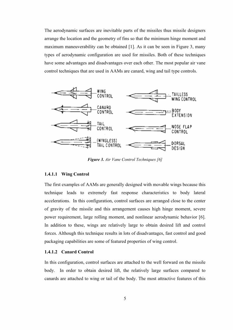
The aerodynamic surfaces are inevitable parts of the missiles thus missile designers
arrange the location and the geometry of fins so that the minimum hinge moment and
maximum maneuverability can be obtained [1]. As it can be seen in Figure 3, many
types of aerodynamic configuration are used for missiles. Both of these techniques
have some advantages and disadvantages over each other. The most popular air vane
control techniques that are used in AAMs are canard, wing and tail type controls.
Figure 3. Air Vane Control Techniques [6]
1.4.1.1 Wing Control
The first examples of AAMs are generally designed with movable wings because this
technique leads to extremely fast response characteristics to body lateral
accelerations. In this configuration, control surfaces are arranged close to the center
of gravity of the missile and this arrangement causes high hinge moment, severe
power requirement, large rolling moment, and nonlinear aerodynamic behavior [6].
In addition to these, wings are relatively large to obtain desired lift and control
forces. Although this technique results in lots of disadvantages, fast control and good
packaging capabilities are some of featured properties of wing control.
1.4.1.2 Canard Control
In this configuration, control surfaces are attached to the well forward on the missile
body. In order to obtain desired lift, the relatively large surfaces compared to
canards are attached to wing or tail of the body. The most attractive features of this
6
configuration are simplicity of packaging, lower missile weight and drag, reduced
power requirement, and lower torque requirements [5]. In addition to these, it easily
compensate the change of center of gravity due to design changes by making simple
relocation of canards. Some of the major disadvantages of this configuration are
difficulty of roll stabilization and high surface rates in order to obtain the desired rate
of response [6]. The most important example of canard control AAMs is Rafael's
Python series.
1.4.1.3 Tail Control
Tail control has slow response characteristic since the tail deflection is in the
opposite direction of the angle of attack so that tail angle of attack and hinge moment
are generally low. Aerodynamic characteristics of this configuration are linear
because wing-tail interference effects are reduced; therefore induced rolling moments
are low [7]. The notable disadvantage is limited space available for the CAS due to
rocket motor and nozzle. In recent years, nearly all AAMs are designed with tail
control.
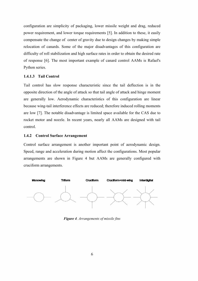
1.4.2 Control Surface Arrangement
Control surface arrangement is another important point of aerodynamic design.
Speed, range and acceleration during motion affect the configurations. Most popular
arrangements are shown in Figure 4 but AAMs are generally configured with
cruciform arrangements.
Figure 4. Arrangements of missile fins
7
1.4.2.1 Monowing
Monowing arrangement is the lightest solution because it contains only two fins. In
this configuration, the missile body is exposed to lower drag than others but wing
areas are wider. This system is widely used in cruise missiles. Turning strategy of
monowing missiles is only bank-to-turn.
1.4.2.2 Triform
In triform arrangement, fins area is nearly equal to the cruciform arrangements. This
arrangement achieves demanded lift and maneuver using three fins. This system
becomes cheaper than cruciform arrangements since the part and actuator numbers
are decreased.
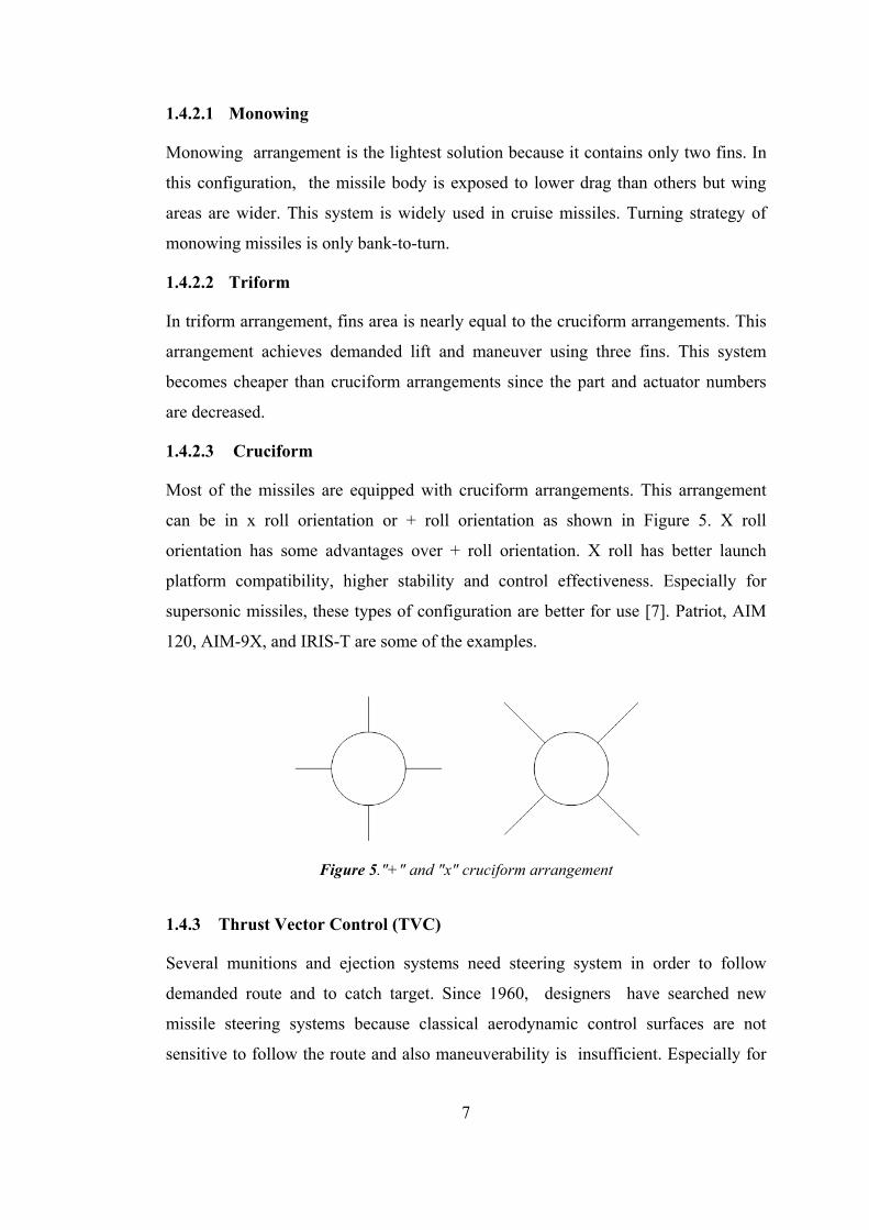
1.4.2.3 Cruciform
Most of the missiles are equipped with cruciform arrangements. This arrangement
can be in x roll orientation or + roll orientation as shown in Figure 5. X roll
orientation has some advantages over + roll orientation. X roll has better launch
platform compatibility, higher stability and control effectiveness. Especially for
supersonic missiles, these types of configuration are better for use [7]. Patriot, AIM
120, AIM-9X, and IRIS-T are some of the examples.
Figure 5."+" and "x" cruciform arrangement
1.4.3 Thrust Vector Control (TVC)
Several munitions and ejection systems need steering system in order to follow
demanded route and to catch target. Since 1960, designers have searched new
missile steering systems because classical aerodynamic control surfaces are not
sensitive to follow the route and also maneuverability is insufficient. Especially for
8
exoatmospheric flight, aerodynamic surfaces become meaningless so these studies
accelerated. Thrust Vector Control (TVC) is the most imported method that was
developed during these studies. In all of the TVC systems; materials, mechanism
design, manufacturing and also aerodynamics design are seen critical technologies.
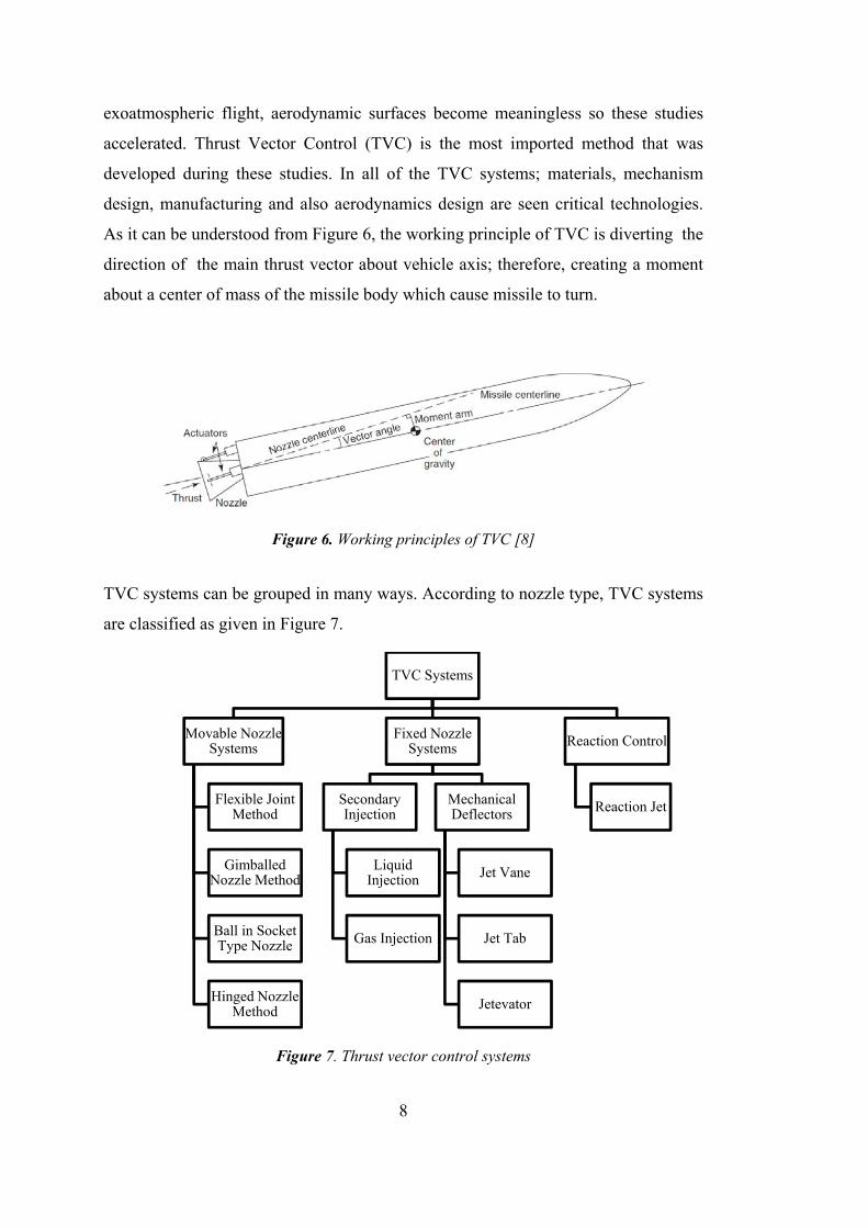
As it can be understood from Figure 6, the working principle of TVC is diverting the
direction of the main thrust vector about vehicle axis; therefore, creating a moment
about a center of mass of the missile body which cause missile to turn.
Figure 6. Working principles of TVC [8]
TVC systems can be grouped in many ways. According to nozzle type, TVC systems
are classified as given in Figure 7.
Figure 7. Thrust vector control systems
TVC Systems
Movable Nozzle Systems
Flexible Joint Method
Gimballed Nozzle Method
Ball in Socket Type Nozzle
Hinged Nozzle Method
Fixed Nozzle Systems
Secondary Injection
Liquid Injection
Gas Injection
Mechanical Deflectors
Jet Vane
Jet Tab
Jetevator
Reaction Control
Reaction Jet
9
TVC systems are used quite a lot in air defense systems, satellite launch rockets,
AAMs, and also intercontinental ballistic missiles. TVC systems have many
advantages for different types of applications, especially for
High speed rockets that require high maneuverability
Manual controlled anti-tank munitions where the aerodynamic control is hard
and speed is low
Vertical launched systems that makes sudden maneuver
Rockets fired from submarines
Air defense system
Platforms like space vehicles where aerodynamic control is impossible and
dynamic pressure is very low.
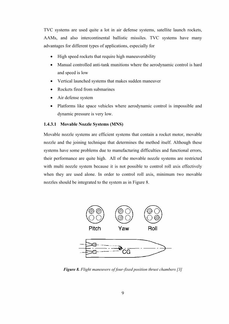
1.4.3.1 Movable Nozzle Systems (MNS)
Movable nozzle systems are efficient systems that contain a rocket motor, movable
nozzle and the joining technique that determines the method itself. Although these
systems have some problems due to manufacturing difficulties and functional errors,
their performance are quite high. All of the movable nozzle systems are restricted
with multi nozzle system because it is not possible to control roll axis effectively
when they are used alone. In order to control roll axis, minimum two movable
nozzles should be integrated to the system as in Figure 8.
Figure 8. Flight maneuvers of four-fixed position thrust chambers [3]
10
In, NASA-SP-8114 [9], TVC systems up to 1974 is examined, and detailed
information about all TVC systems is given. According to [9], nearly more than half
of the TVC system designed was only tested in laboratory environment; therefore, in
this thesis, only tested and applied methods are mentioned briefly. When movable
nozzle systems are investigated, it is understood that these systems are generally used
in satellite launch rocket, large diameter ballistic missiles and air defense systems.
Difference from the other systems, air defense systems are supported with buster
which is ejected after missile reaches desired altitude. Movable nozzle TVC systems
are divided into four groups according to the mechanisms.
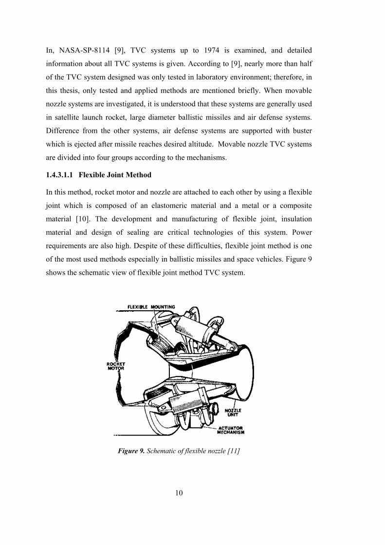
1.4.3.1.1 Flexible Joint Method
In this method, rocket motor and nozzle are attached to each other by using a flexible
joint which is composed of an elastomeric material and a metal or a composite
material [10]. The development and manufacturing of flexible joint, insulation
material and design of sealing are critical technologies of this system. Power
requirements are also high. Despite of these difficulties, flexible joint method is one
of the most used methods especially in ballistic missiles and space vehicles. Figure 9
shows the schematic view of flexible joint method TVC system.
Figure 9. Schematic of flexible nozzle [11]
11
1.4.3.1.2 Gimbaled Nozzle Method
The nozzle is fastened to the rocket motor via gimbal mechanisms. In this method,
thrust loss is quite small but the sliding motion of the gimbal which makes it difficult
to maintain sealing. Reliability of these systems depends on whether or not the
sealing is designed well. Because of these, this method is not preferred in tactical
missile systems.
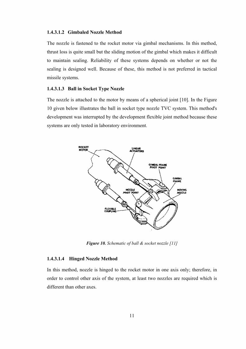
1.4.3.1.3 Ball in Socket Type Nozzle
The nozzle is attached to the motor by means of a spherical joint [10]. In the Figure
10 given below illustrates the ball in socket type nozzle TVC system. This method's
development was interrupted by the development flexible joint method because these
systems are only tested in laboratory environment.
Figure 10. Schematic of ball & socket nozzle [11]
1.4.3.1.4 Hinged Nozzle Method
In this method, nozzle is hinged to the rocket motor in one axis only; therefore, in
order to control other axis of the system, at least two nozzles are required which is
different than other axes.
12
1.4.3.2 Fixed Nozzle Systems
Fixed nozzle system systems change the direction of thrust vector using secondary
fluid injection and mechanical deflectors [8, 12]. Both of these methods have some
use in many applications. In most cases, application systems are different than each
other while mechanical deflectors are used in small diameter systems like air to air
missile, secondary injection methods are preferred in ballistic missiles and large
diameter rockets.
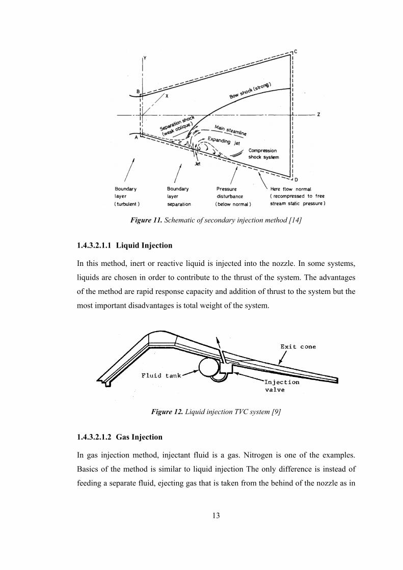
1.4.3.2.1 Secondary Injection Thrust Vector Control (SITVC)
In secondary injection method, flow manipulation is accomplished by injecting a
secondary fluid inside to the nozzle as shown in Figure 11 which creates shock
waves [4-8]. In this way, symmetry of pressure difference on inner wall of nozzle is
broken down which expand the flow to the side of the nozzle thus, this action cause a
side force on nozzle. This side force forms the thrust vector deflection. SITVC does
not need any moving part; therefore, thrust losses are less than mechanically
operating TVC systems. SITVC is chosen especially for ballistic missiles and launch
systems. SITVC is carried out by different methods [13]. The easiest one is taking
secondary injectant from main rocket motor. Another method is using different
injectant. In this method, liquid or gas is ejected to the nozzle from a pressurized
vessel. The selection of injectant, location of jet, amount of fluid, the selection and
number of orifice and the related equipment are important design criteria. SITVC
makes some combinations including different types of injectors, injectant fluids,
injection location, angle of injection, and types of pressure vessel in order to apply
the optimal solution to the specified system.
13
Figure 11. Schematic of secondary injection method [14]
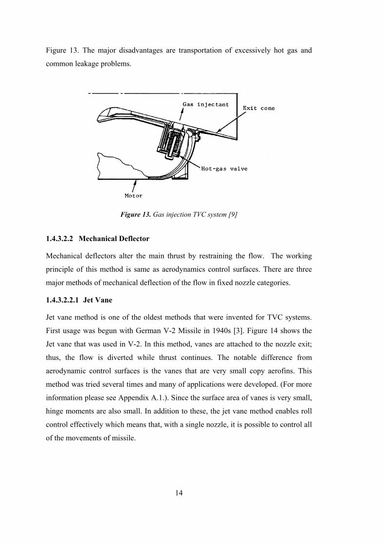
1.4.3.2.1.1 Liquid Injection
In this method, inert or reactive liquid is injected into the nozzle. In some systems,
liquids are chosen in order to contribute to the thrust of the system. The advantages
of the method are rapid response capacity and addition of thrust to the system but the
most important disadvantages is total weight of the system.
Figure 12. Liquid injection TVC system [9]
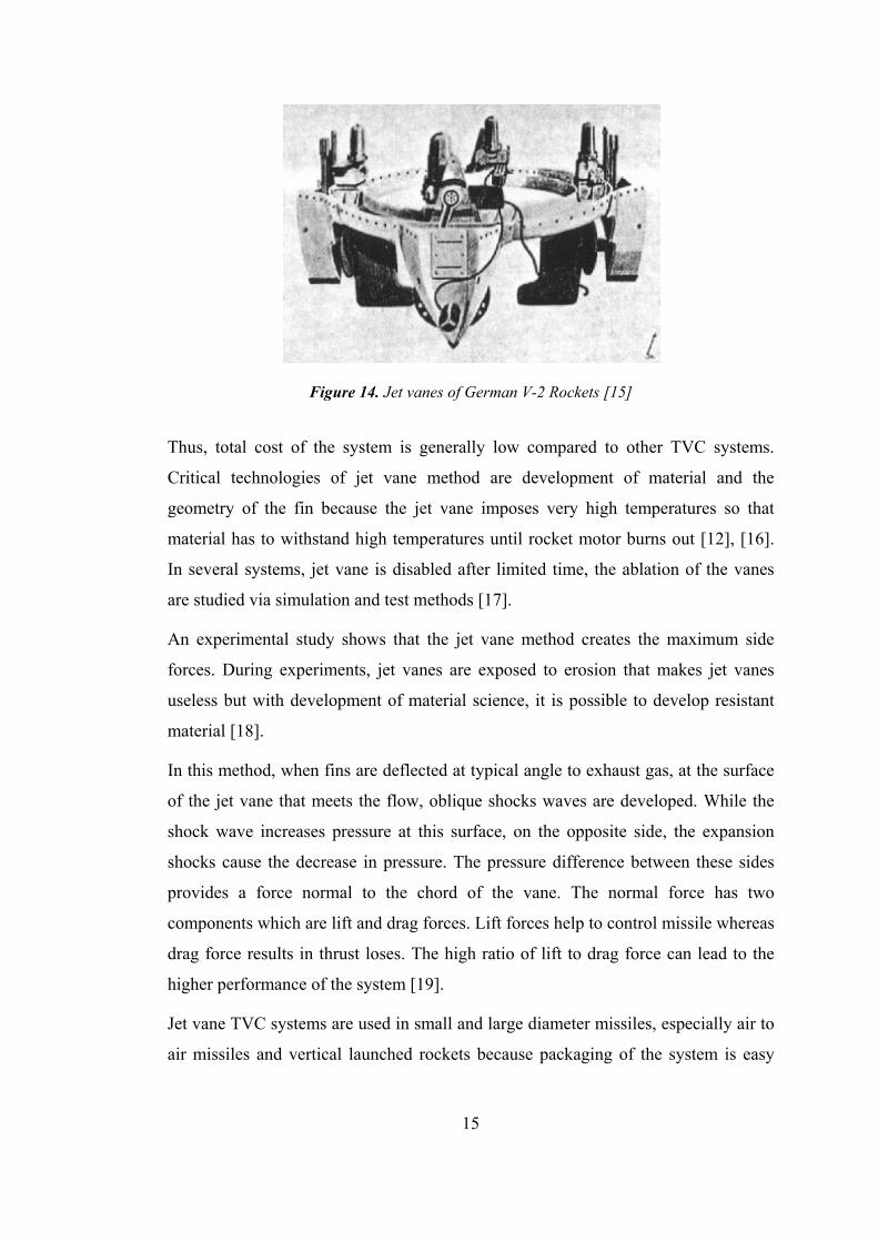
1.4.3.2.1.2 Gas Injection
In gas injection method, injectant fluid is a gas. Nitrogen is one of the examples.
Basics of the method is similar to liquid injection The only difference is instead of
feeding a separate fluid, ejecting gas that is taken from the behind of the nozzle as in
14
Figure 13. The major disadvantages are transportation of excessively hot gas and
common leakage problems.
Figure 13. Gas injection TVC system [9]
1.4.3.2.2 Mechanical Deflector
Mechanical deflectors alter the main thrust by restraining the flow. The working
principle of this method is same as aerodynamics control surfaces. There are three
major methods of mechanical deflection of the flow in fixed nozzle categories.
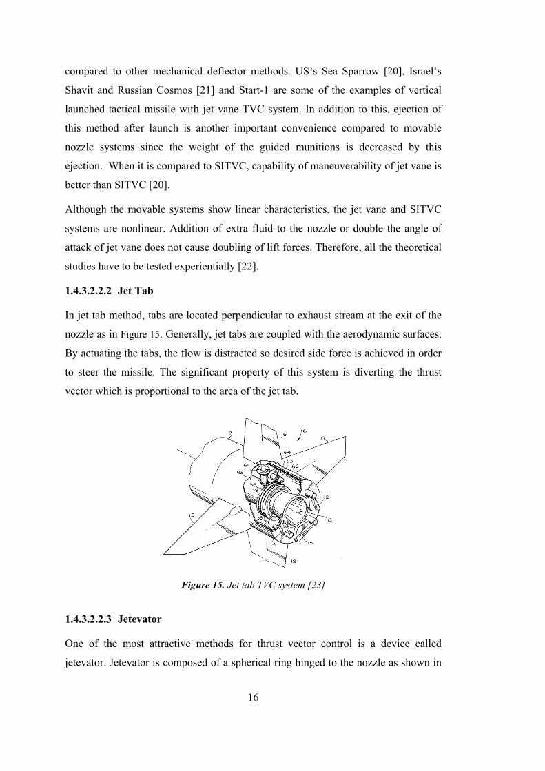
1.4.3.2.2.1 Jet Vane
Jet vane method is one of the oldest methods that were invented for TVC systems.
First usage was begun with German V-2 Missile in 1940s [3]. Figure 14 shows the
Jet vane that was used in V-2. In this method, vanes are attached to the nozzle exit;
thus, the flow is diverted while thrust continues. The notable difference from
aerodynamic control surfaces is the vanes that are very small copy aerofins. This
method was tried several times and many of applications were developed. (For more
information please see Appendix A.1.). Since the surface area of vanes is very small,
hinge moments are also small. In addition to these, the jet vane method enables roll
control effectively which means that, with a single nozzle, it is possible to control all
of the movements of missile.
15
Figure 14. Jet vanes of German V-2 Rockets [15]
Thus, total cost of the system is generally low compared to other TVC systems.
Critical technologies of jet vane method are development of material and the
geometry of the fin because the jet vane imposes very high temperatures so that
material has to withstand high temperatures until rocket motor burns out [12], [16].
In several systems, jet vane is disabled after limited time, the ablation of the vanes
are studied via simulation and test methods [17].
An experimental study shows that the jet vane method creates the maximum side
forces. During experiments, jet vanes are exposed to erosion that makes jet vanes
useless but with development of material science, it is possible to develop resistant
material [18].
In this method, when fins are deflected at typical angle to exhaust gas, at the surface
of the jet vane that meets the flow, oblique shocks waves are developed. While the
shock wave increases pressure at this surface, on the opposite side, the expansion
shocks cause the decrease in pressure. The pressure difference between these sides
provides a force normal to the chord of the vane. The normal force has two
components which are lift and drag forces. Lift forces help to control missile whereas
drag force results in thrust loses. The high ratio of lift to drag force can lead to the
higher performance of the system [19].
Jet vane TVC systems are used in small and large diameter missiles, especially air to
air missiles and vertical launched rockets because packaging of the system is easy
16
compared to other mechanical deflector methods. US’s Sea Sparrow [20], Israel’s
Shavit and Russian Cosmos [21] and Start-1 are some of the examples of vertical
launched tactical missile with jet vane TVC system. In addition to this, ejection of
this method after launch is another important convenience compared to movable
nozzle systems since the weight of the guided munitions is decreased by this
ejection. When it is compared to SITVC, capability of maneuverability of jet vane is
better than SITVC [20].
Although the movable systems show linear characteristics, the jet vane and SITVC
systems are nonlinear. Addition of extra fluid to the nozzle or double the angle of
attack of jet vane does not cause doubling of lift forces. Therefore, all the theoretical
studies have to be tested experientially [22].
1.4.3.2.2.2 Jet Tab
In jet tab method, tabs are located perpendicular to exhaust stream at the exit of the
nozzle as in Figure 15. Generally, jet tabs are coupled with the aerodynamic surfaces.
By actuating the tabs, the flow is distracted so desired side force is achieved in order
to steer the missile. The significant property of this system is diverting the thrust
vector which is proportional to the area of the jet tab.
Figure 15. Jet tab TVC system [23]
1.4.3.2.2.3 Jetevator
One of the most attractive methods for thrust vector control is a device called
jetevator. Jetevator is composed of a spherical ring hinged to the nozzle as shown in
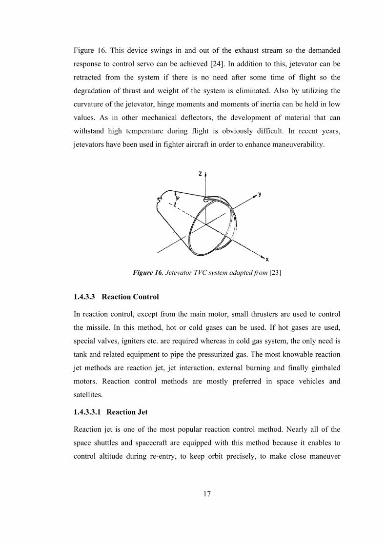
17
Figure 16. This device swings in and out of the exhaust stream so the demanded
response to control servo can be achieved [24]. In addition to this, jetevator can be
retracted from the system if there is no need after some time of flight so the
degradation of thrust and weight of the system is eliminated. Also by utilizing the
curvature of the jetevator, hinge moments and moments of inertia can be held in low
values. As in other mechanical deflectors, the development of material that can
withstand high temperature during flight is obviously difficult. In recent years,
jetevators have been used in fighter aircraft in order to enhance maneuverability.
Figure 16. Jetevator TVC system adapted from [23]
1.4.3.3 Reaction Control
In reaction control, except from the main motor, small thrusters are used to control
the missile. In this method, hot or cold gases can be used. If hot gases are used,
special valves, igniters etc. are required whereas in cold gas system, the only need is
tank and related equipment to pipe the pressurized gas. The most knowable reaction
jet methods are reaction jet, jet interaction, external burning and finally gimbaled
motors. Reaction control methods are mostly preferred in space vehicles and
satellites.
1.4.3.3.1 Reaction Jet
Reaction jet is one of the most popular reaction control method. Nearly all of the
space shuttles and spacecraft are equipped with this method because it enables to
control altitude during re-entry, to keep orbit precisely, to make close maneuver

18
during docking procedures, to control orientation, to point the nose of the craft and
finally in order to deorbit the system [25]. Another application area of the reaction jet
is projectiles or mortars. In these systems, reaction jets are placed aft section of the
body to achieve the desired directional control of the system. General view is that the
reaction control decreases the control accuracy for such systems but the main idea
here is not to control system precisely only to increase turning capabilities in limited
area [26]. In these systems, one shot squibs or pulsed unit are used. [27].
Figure 17. Projectile reaction jet control system adapted from [27]
1.5 Basic Concepts of Hybrid Fin Actuation Systems
Fin actuation systems are inevitable parts of missiles. According to applications
some systems have different types of control methods as mentioned before. The
combination of these methods is called as hybrid fin actuation systems. The elements
of methods can be any configuration. The important point of hybrid fin actuation
system is being able to control a system without using more than one actuator for a
single fin. To illustrate it, if rocket motors burns in 10s, after that since there is no
exhaust flow to control, rocket designer needs conventional control method to steer
missile during flight. At this point, the movable aerodynamic control surfaces are
indispensable. In order to compose conventional aerodynamic control and TVC,
different attempts are made [23], [28], [29], [30],[31]. Nowadays, air to air missiles
are equipped with these systems and most of them use jet vanes or jet tabs with aero-
fins. The implantation of these mechanisms to the system is easy and cost effective;
therefore, most advanced air to air missiles such as AIM 9X and IRST-T are
designed with hybrid fin actuation systems. In this thesis, aerodynamic control
surfaces are coupled with jet vanes.
19
1.6 Review of the Literature on H∞ Control
H∞ control theory is a branch of Robust Control Theory. In order to use H∞ method,
control engineers express the problem statement as mathematical optimization
problem and the try to find a controller. In this section, brief history and theory of
robust control will be explained.
1.6.1 Historical Background
Control theory is inevitable part of our life. Without control system, it is not possible
to develop technologies [32]. All the technologies that surround us are the results of
control theory. Control theory can be divided into two main areas which are classical
and modern control theories. Although the classical control theory has been used for
centuries, the modern control theory is developed around 1950s. With the
introduction of Pontryagin's maximum principle in 1956, dynamic programming by
Bellman in 1957, and state space representation by Kalman in 1959, modern control
theory was founded [33]. The developments of modern control theory opened a new
era of control system which is called Robust Control Theory in 1981. The first
investigation of the robust control theory was started with Zames [34], where H∞
optimal control problem was formulated. Then, Doyle at all introduces a state space
solution to such problems in 1989 [35] . After that robust control theory has being
developed.
1.7 Theoretical Background of Robust Control
Robust control means synthesis of a controller such that this controller makes system
stable and guarantees some performance characteristics for an unknown plant with
unknown dynamics which is subjected to unknown disturbances [36]. These
uncertainties can be any form, but the most important ones are sensor noise,
nonlinearity of the system, and unknown dynamics of the plant. In this section,
concepts used in robust control are given.
1.7.1 Reasons for Robust Control
For many engineering problems, classical control methods are sufficient enough, but
for some systems these methods cannot be defined well or fail to satisfy some
20
requirements so that designed controller could not provide desired performance. This
is because of unknown dynamics and disturbances. In such cases, more powerful
design techniques are preferred. The main idea of the robust control is to be
insensitive to variation of parameters and able to maintain its stability and
performance. The designed controllers meet the desired system requirements in all
cases. For that reason sometimes robust control theory are specified as worst case
analysis method [36].
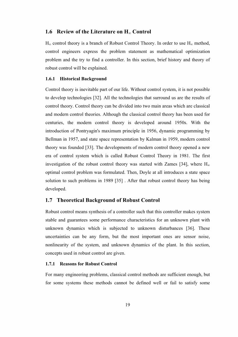
1.7.2 Problem Statement
In order to define problem in robust control theory, the following block diagram
which is given in Figure 18 is used.
Figure 18. Standard LTI feedback block diagram
In Figure 18, G is called generalized plant and K is the controller. The input w is
called the disturbance and it contains all the external inputs including reference
signals and external noises. The second input u is called actuator and represents the
controller signal. The first output z is called cost and represents the error signals
which are wanted to be low. And finally, the last output y represents the
measurement signals. In this thesis, all the systems are assumed as finite order, linear
and time invariant (LTI) according to the formulation given above. The aim is trying
to find a controller which makes the system stable and minimize the norms of
transfer functions from inputs to errors.
21
1.7.3 Norms of Systems
In Robust Control Theory, norms are one of the ways that are used to describe the
performance and stability of the system. In order to define norm, a real-valued
function ||·|| is used if it satisfies the following properties [32].
i. || || 0 x (positivity) (1.1)
ii. || || 0 iff 0x x (positive definiteness) (1.2)
iii. || || | | ||x||x for any scalar (homogeneity) (1.3)
iv. || || || || + || y ||x y x (triangle inequality) (1.4)
for any nx and y X .
Some signals need special attention for analysis and synthesis. In order to define
norm of a system, root-mean-square (RMS) value is needed. Root mean square value
is a common method to measure the size of the energy of the signal. [37].
2
0
1|| || lim (t)
T
Tu u dt
T (1.5)
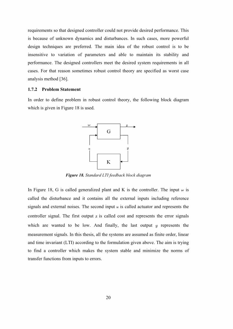
The RMS value of the system in Figure 19, formulated in frequency domain, then
RMS value of the system can also be given as [37].
21|| || | G( ) | ( )
2rmsG j S d
(1.6)
Figure 19. System G(s) operating on signal w(s)
where ( )S is the power spectral density of the input. Using above formulation
various norms can be defined such as 2H , H etc. In this thesis, H norm is used for
optimization procedure. H norm is the maximum magnitude of the G on imaginary
G z w
22
axis which is given as Eq. (1.7)
|| || sup | G(j ) |G
(1.7)
1.7.4 Linear Fractional Transformation (LFT)
The LFT has a useful representation that was introduced by Doyle [35]. Consider a
plant matrix given in equation (1.8)
1: (sI A)A B
C B DC D
(1.8)
Applying LTI representation to general framework given in Figure 18. According to
the given input and out signals, the following relation can be obtained.
11 12
21 22
P PP
P P
(1.9)
11 12
21 22
P Pz w
P Py u
(1.10)
The transformation from input u to output z is called the lower linear fractional
transformation.
(P, K) wzw lz T w F (1.11)
where
111 21 22 21( , ) ( )zw lT F P K P P K I P K P (1.12)
Similarly, upper fractional transformation is found for the system given in Figure 20.
122 21 11 12( , ) ( )uF P P P K I P K P (1.13)
23
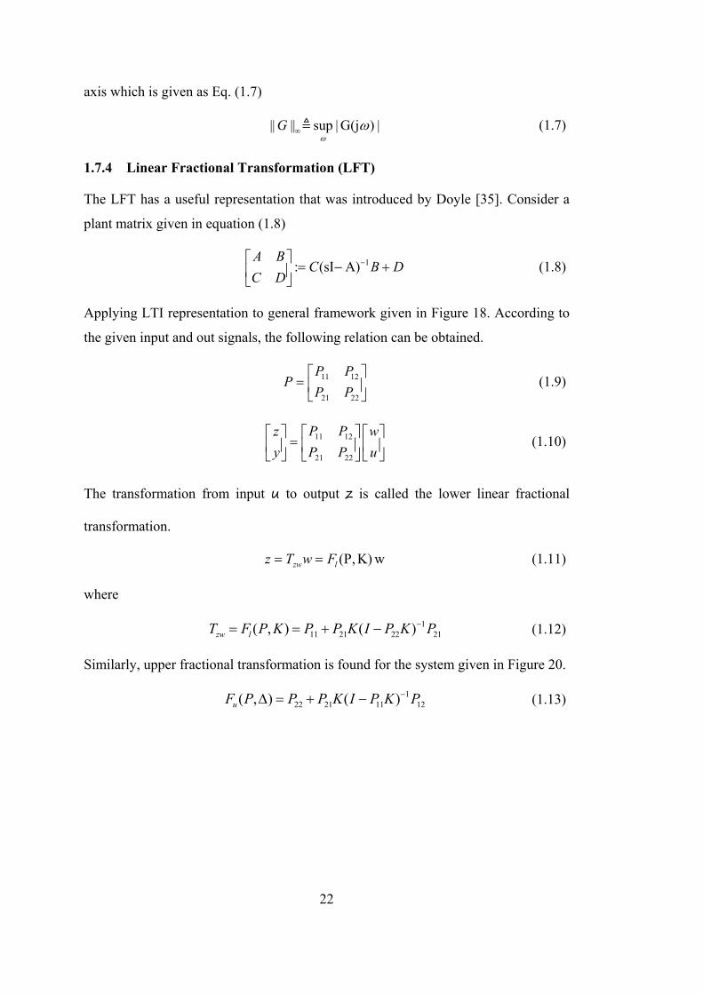
Figure 20. Upper fractional transformation
The H control problem tries to find a controller that minimizes the infinity norm of
an input output map zwT or || ||zwT [38].
1.7.5 Sensitivity, Robustness and Feedback Structure
After making all the transformation according to LTF representation, control system
can be shown as in Figure 21.
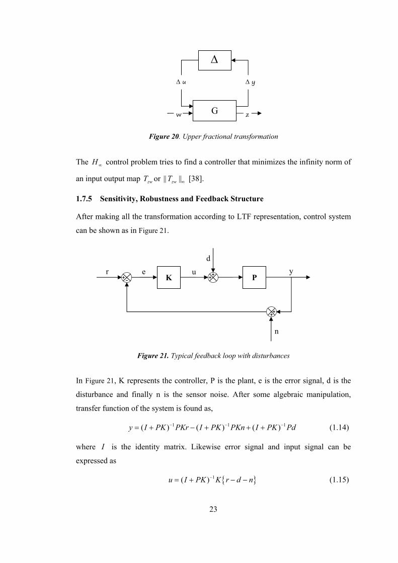
Figure 21. Typical feedback loop with disturbances
In Figure 21, K represents the controller, P is the plant, e is the error signal, d is the
disturbance and finally n is the sensor noise. After some algebraic manipulation,
transfer function of the system is found as,
1 1 1( ) ( ) ( )y I PK PKr I PK PKn I PK Pd (1.14)
where I is the identity matrix. Likewise error signal and input signal can be
expressed as
1( )u I PK K r d n (1.15)
K P r
n
y
d
e u
G
w z
y u
24
1( )e I PK r d n (1.16)
In control terminology, PK is called loop transfer matrix, 1( )I PK is called output
sensitivity matrix 'S' and 1( )I PK PK is called complementary output transfer
matrix 'T'.
1
SI PK
(1.17)
PK
TI PK
(1.18)
The complementary terms comes from the equality;
S T I (1.19)
S indicates output disturbance input d to the output y. It also describes the tracking
error to the reference input. T relates the output of the system to the reference signal.
It also indicates how the output is affected by the noise. In a good controller
synthesis problem, feedback control system include stability, command following,
disturbance rejection, sensor noise attenuation and minimization of control
sensitivity. For good command following and disturbance rejection, outputs should
track the input reference signals and disturbances inputs have negligible effects upon
the outputs. In order to achieve this which means that (s) r(s)y and (s) 0e , S
should be minimized 0S and T I . For control sensitivity and robustness, T
must be small ' 0T '. As can be understood from the relation of S and T, both good
tracking and noise/disturbance attenuation can be accomplished at the same time. In
order to optimize this trade off, one should make the required changes at different
frequencies. For low frequencies, T should be made high enough so the disturbance
effects are diminished. For high frequencies, T should be small in order to attenuate
noise. For detailed information please refer to [38] and [39].
1.7.6 Plant Uncertainty, Stability and Performance
Uncertainty is defined as difference or error between the model and real system. The
source of uncertainty may vary from system to system. In some linear system,
parameters are known approximately or there can be an error in parameters. Due to
25
changes and nonlinearities, these parameters may vary again. Another source can be
imperfection of measurement devices such as accuracy, linearity, mounting errors
etc. These can cause rise an uncertainty on the manipulated inputs. In addition to this,
at high frequencies, plant dynamics may be different than identified one. The
uncertainty may exceed 100% at some frequency. In some application, although
detailed model is available, model reduction techniques can be applied so that some
of the dynamics are neglected. These neglected dynamics are also referred as
uncertainty. Finally, implementation of controller to the system may differ from the
synthesized one. This situation leads to uncertainty in the real system. All these
uncertainties may be classified into two main areas [39]:
1. Parametric uncertainty
In parametric uncertainty, some parameters of the system are unknown.
These unknown parameters may be defined in some bounded region
min max[ , ] than parameter set is defined as
[1 ]px x r (1.20)
where x is mean value, 1 is any scalar and
max min
max max
r
(1.21)
2. Neglected and unmodelled uncertainty
In system, some phenomena are not fully understood so that some of the
parameters of the model are missing, usually at high frequencies. Any model
will include such type of an uncertainty. These uncertainties may not be
defined as in parametric uncertainty.
There are two ways in order to describe uncertainty in a system which are
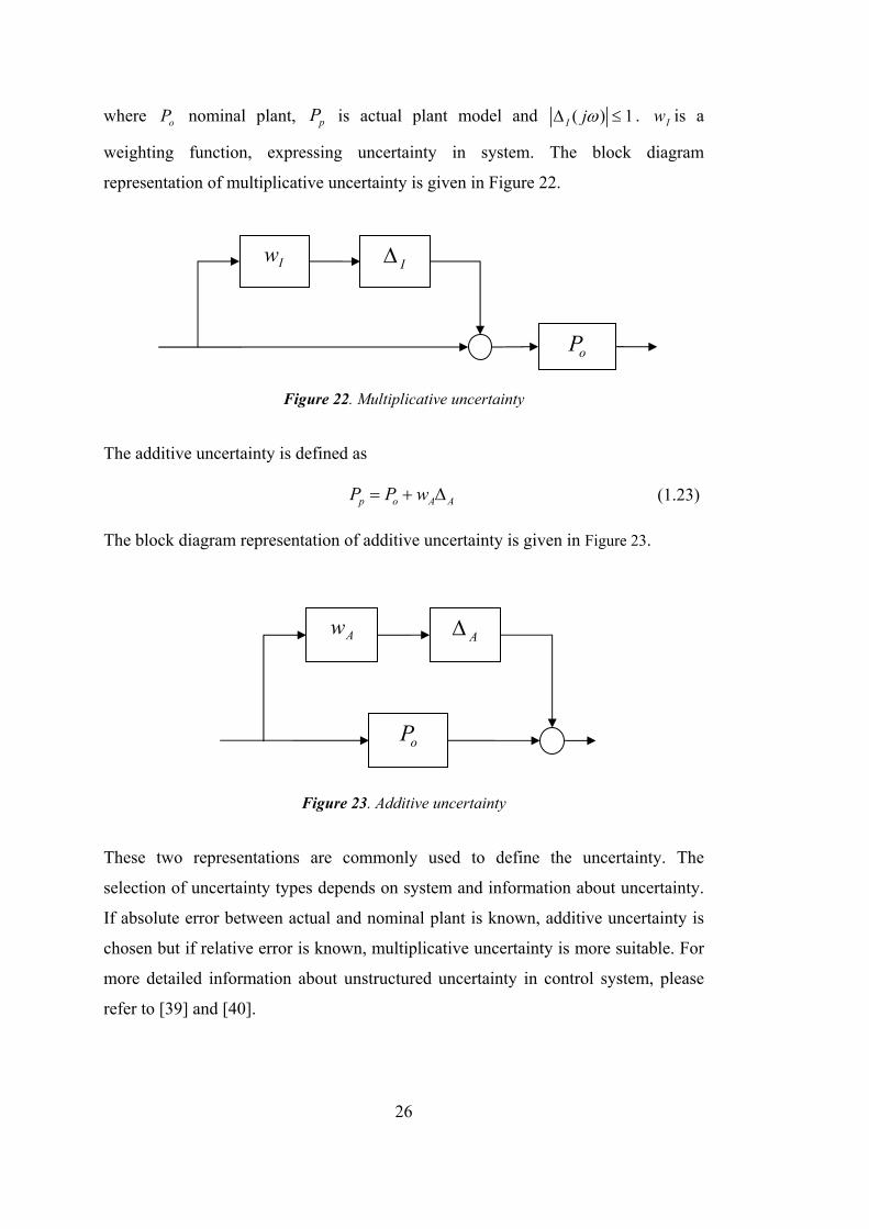
multiplicative and additive uncertainty. The multiplicative uncertainty is expressed
as
( )p o I IP P I w (1.22)
26
where oP nominal plant, pP is actual plant model and ( ) 1I j . Iw is a
weighting function, expressing uncertainty in system. The block diagram
representation of multiplicative uncertainty is given in Figure 22.
Figure 22. Multiplicative uncertainty
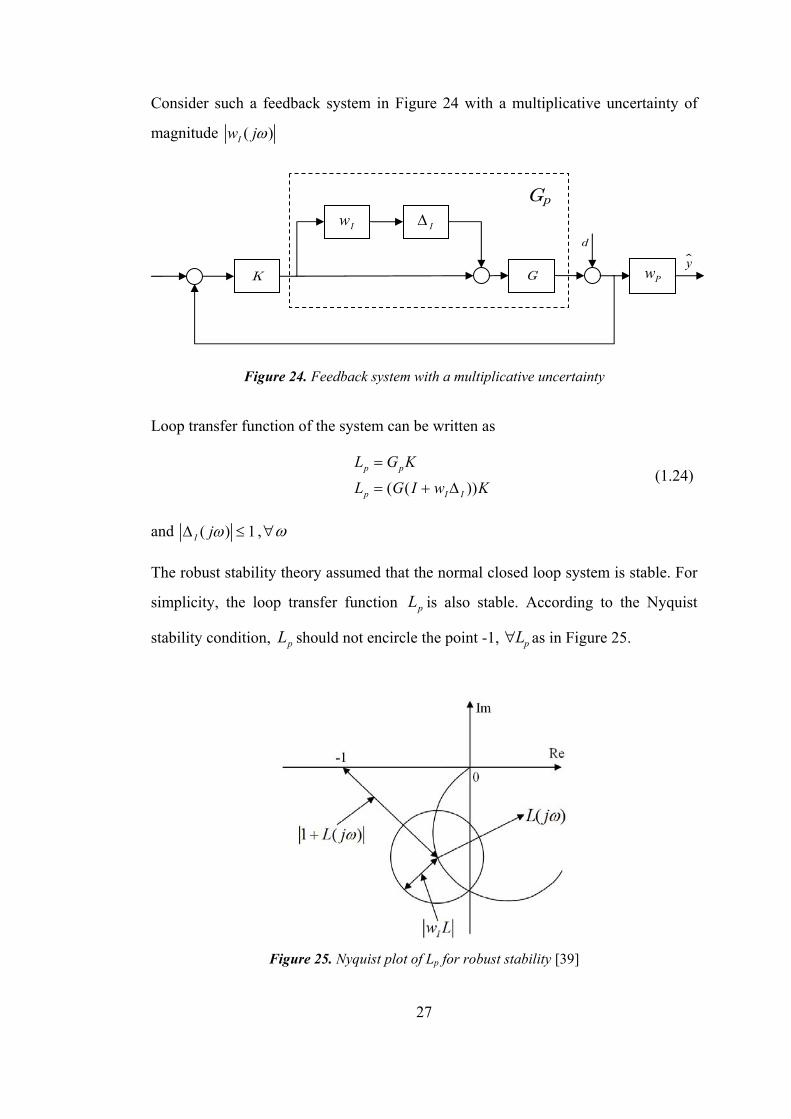
The additive uncertainty is defined as
p o A AP P w (1.23)
The block diagram representation of additive uncertainty is given in Figure 23.
Figure 23. Additive uncertainty
These two representations are commonly used to define the uncertainty. The
selection of uncertainty types depends on system and information about uncertainty.
If absolute error between actual and nominal plant is known, additive uncertainty is
chosen but if relative error is known, multiplicative uncertainty is more suitable. For
more detailed information about unstructured uncertainty in control system, please
refer to [39] and [40].
A
oP
Aw
I
oP
Iw
27
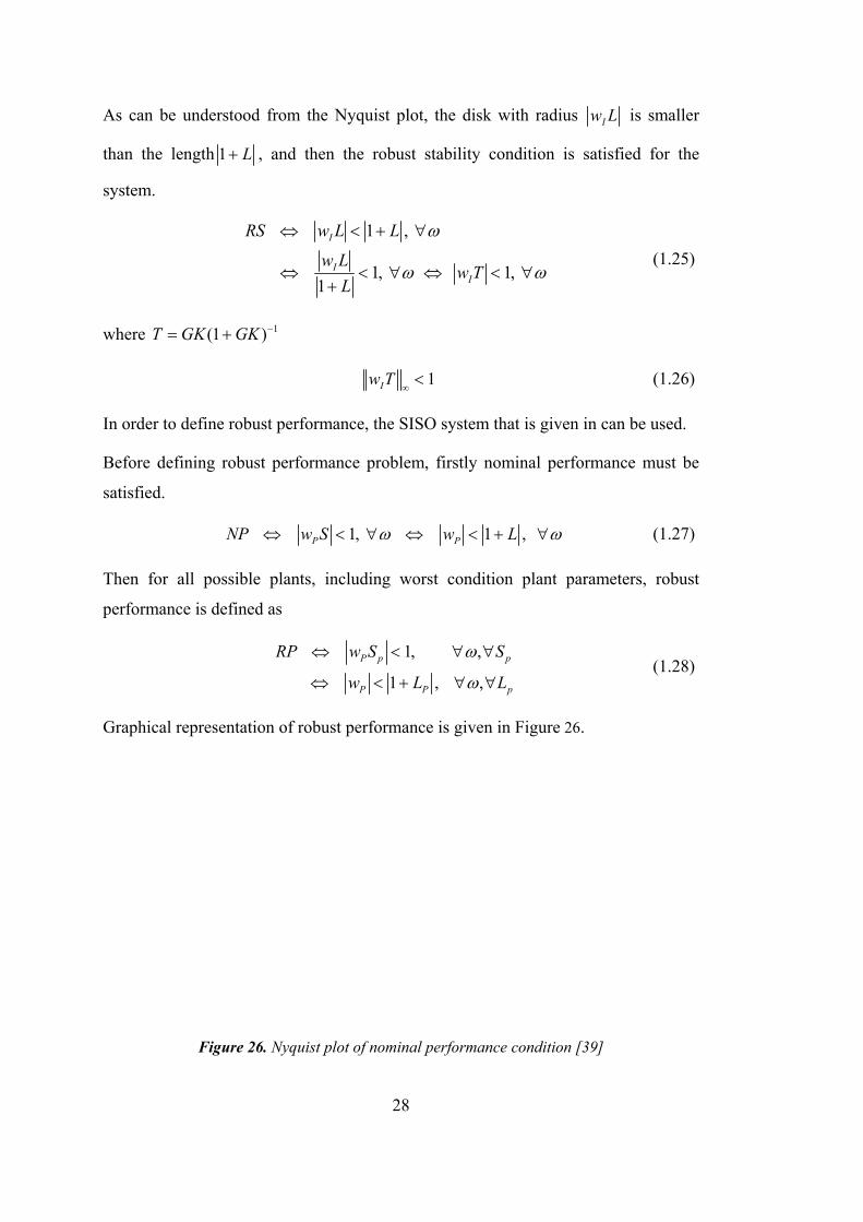
Consider such a feedback system in Figure 24 with a multiplicative uncertainty of
magnitude ( )Iw j
Figure 24. Feedback system with a multiplicative uncertainty
Loop transfer function of the system can be written as
( ( ))
p p
p I I
L G K
L G I w K
(1.24)
and ( ) 1I j ,
The robust stability theory assumed that the normal closed loop system is stable. For
simplicity, the loop transfer function pL is also stable. According to the Nyquist
stability condition, pL should not encircle the point -1, pL as in Figure 25.
Figure 25. Nyquist plot of Lp for robust stability [39]
yd
I
G
Iw
K
Pw
Gp
28
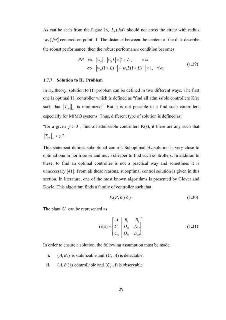
As can be understood from the Nyquist plot, the disk with radius Iw L is smaller
than the length 1 L , and then the robust stability condition is satisfied for the
system.
1 ,
1, 1, 1
I
II
RS w L L
w Lw T
L
(1.25)
where 1(1 )T GK GK
1Iw T (1.26)
In order to define robust performance, the SISO system that is given in can be used.
Before defining robust performance problem, firstly nominal performance must be
satisfied.
1, 1 , P PNP w S w L (1.27)
Then for all possible plants, including worst condition plant parameters, robust
performance is defined as
1, ,
1 , ,
P p p
P P p
RP w S S
w L L
(1.28)
Graphical representation of robust performance is given in Figure 26.
Figure 26. Nyquist plot of nominal performance condition [39]
29
As can be seen from the Figure 26, ( )PL j should not cross the circle with radius
( )Pw j centered on point -1. The distance between the centers of the disk describe
the robust performance, then the robust performance condition becomes
1 1
1 ,
(1 ) (1 ) 1,
P I
P I
RP w w L L
w L w L L
(1.29)
1.7.7 Solution to H∞ Problem
In H∞ theory, solution to H∞ problem can be defined in two different ways. The first
one is optimal H∞ controller which is defined as "find all admissible controllers K(s)
such that zwT
is minimized". But it is not possible to a find such controllers
especially for MIMO systems. Thus, different type of solution is defined as:
"for a given 0 , find all admissible controllers K(s), it there are any such that
zwT ".
This statement defines suboptimal control. Suboptimal H∞ solution is very close to
optimal one in norm sense and much cheaper to find such controllers. In addition to
these, to find an optimal controller is not a practical way and sometimes it is
unnecessary [41]. From all these reasons, suboptimal control solution is given in this
section. In literature, one of the most known algorithms is presented by Glover and
Doyle. This algorithm finds a family of controller such that
( , )lF P K (1.30)
The plant G can be represented as
1 1
1 11 12
2 21 22
( )
A B B
G s C D D
C D D
(1.31)
In order to ensure a solution, the following assumption must be made
i. 2( , )A B is stabilizable and 2( , )C A is detectable.
ii. 1( , )A B is controllable and 1( , )C A is observable.
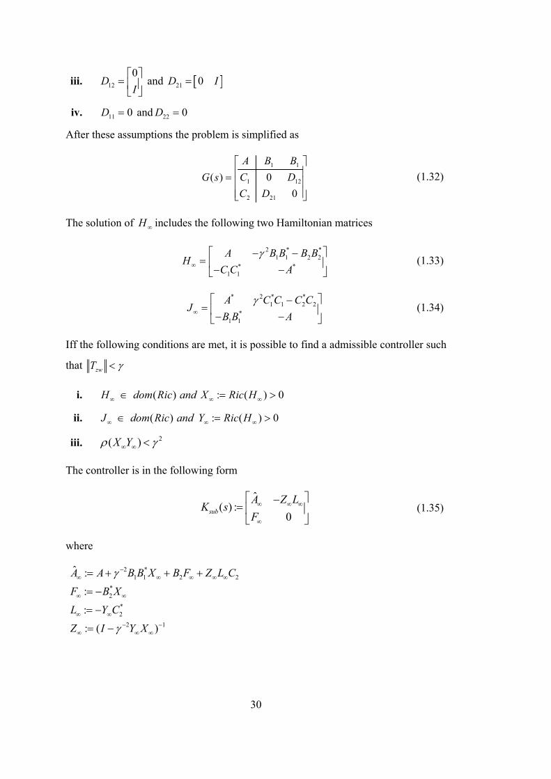
30
iii. 12
0D
I
and 21 0D I
iv. 11 0D and 22 0D
After these assumptions the problem is simplified as
1 1
1 12
2 21
( ) 0
0
A B B
G s C D
C D
(1.32)
The solution of H includes the following two Hamiltonian matrices
2 * *
1 1 2 2* *
1 1
A B B B BH
C C A
(1.33)
* 2 * *
1 1 2 2*
1 1
A C C C CJ
B B A
(1.34)
Iff the following conditions are met, it is possible to find a admissible controller such
that zwT
i. ( ) : ( ) 0H dom Ric and X Ric H
ii. ( ) : ( ) 0J dom Ric and Y Ric H
iii. 2( )X Y
The controller is in the following form
ˆ
( ) :0
sub
A Z LK s
F
(1.35)
where
2 *1 1 2 2
*2
*2
2 1
ˆ :
:
:
: ( )
A A B B X B F Z L C
F B X
L Y C
Z I Y X

31
1.8 Literature Review of the Electro-Mechanical Actuator Control
In many aerospace applications such as missile, aircraft etc., electromechanical
actuators are widely used; therefore in literature there are numerous papers about
electromechanical actuator control. In this section, previous works about
electromechanical actuators especially for missile fin control are given.
In 1992, Hartley designed a reduced fourth order H∞ controller for electromechanical
actuator of tail control missile whose frequency response characteristic is similar to
seventh-order H∞. With this work Hartley intends to reduce requirements of
microprocessor [42]. In 1993, Hartley tested a H∞ controller on single axis prototype
electromechanical actuator and made some comparison between classical and H∞
controller design [43]. In 1994, Malassé at all designed an H∞ control law for a
testing bench which is based on coprime factors and compared obtained results with
LQG and LQR/LTR designs [44]. Adam and Guestrin made experimental studies on
servo motors. They designed a robust controller and stated the results about the
performance of their system [45]. Luo and Fan (2003) [46] and Ölçer [47] introduced
a mixed H2 / H∞ controller that combines both H2 performance and H∞ stability for
missile electromechanical actuator. They showed simulation and analytical results to
the change of parameter and perturbation. Daş [48] made experiments on fin
actuation system and presented the multi-loop robust controller. Yoo at all designed
an H∞ controller for an electromechanical fin actuator system using the mixed
sensitivity H∞ control method. The effectiveness of the controller was verified
through simulations and experiments [49]. In 2006, Eker studied a sliding mode
controller with PID sliding surface and applied his controller to an electromechanical
actuator test bench. He compared the solutions with conventional PID and showed
controller's tracking performance and robustness [50]. One of the most notable
studies about electromechanical actuator is made by Schinstock at all They
developed a nonlinear model of thrust vector control of rocket engines and made
experiment to verify the model of the actuator [51] [52] [53]. Other important studies
were presented by Ristanović. They made experimental studies to improve the
performance of the aerofin control system using both conventional and modern
control techniques. They tried intelligent control techniques and nonlinear PID

32
controllers to validate their research experimentally [54] [55] [56] [57]. In addition to
these, some applications are achieved by using DSP. Jeong at all (2007) [58] and
Khan, Todic, Milos, Stefanovic, Blagojevic (2010) [59] made research about digital
controllers and propose a controller for digitally controlled missile actuator. Beside
these, variable structure control is used in missile actuators. Robustness of a variable
structure makes it important. Gao, Gu and Pan (2008) [60] and Li and Sun (2010)
[61], Liu, Wu, Deng and Xiao [62] made research on variable structure control.
33
CHAPTER 2
SYSTEM MODELING AND IDENTIFICATION
2.1 Modeling of the System
Fin actuation systems steer the missile according to the commands taken from the
guidance unit. The output of the guidance unit is the reference input to the control
unit which adjusts the position of the fin actuation elements such that a missile tracks
the commanded motion as closely as possible. The fin actuation system (FAS) is a
closed loop type control unit since the information of the actual position of fins is
supplied to the control unit by the position sensors. Then the fin deflection data are
taken by the guidance autopilot. The related calculation is made according to the
aerodynamics principles in guidance unit. After that, autopilot finds the deviation
from the target using its gyroscope and accelerometer data. In order to enhance the
precision level of target tracking, other type of sensors are used which is called as
seeker unit of missile. Seekers can be IR, IIR, radar antennas or laser. These seekers
can be used individually or used together as in dual mode seeker. Finally, the
corrected fin position command is generated by the autopilot and this procedure
continues until the missile hits the target.
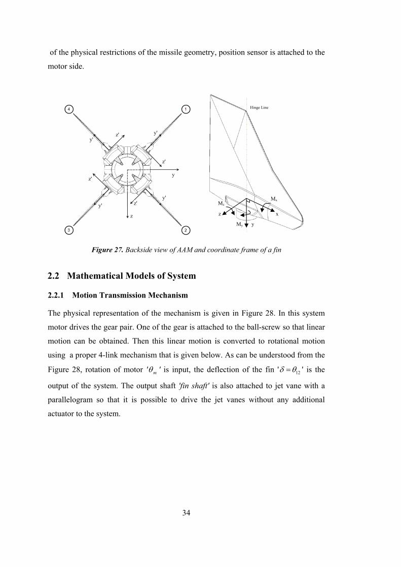
The surface arrangement of the AAM is cruciform X-arrangement as presented in
section (1.4.2). The back side view of the missile given in Figure 27. During the
flight of the missile, fin actuation system must overcome the forces shown in Figure
27. In this study, fin actuation system is composed of brushless DC motor (BLDC), a
position sensor, gear train and a proper 4-link (PPRR linkage) mechanism. Because
34
of the physical restrictions of the missile geometry, position sensor is attached to the
motor side.
Figure 27. Backside view of AAM and coordinate frame of a fin
2.2 Mathematical Models of System
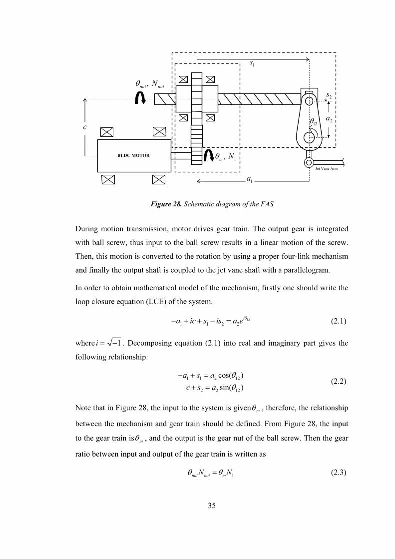
2.2.1 Motion Transmission Mechanism
The physical representation of the mechanism is given in Figure 28. In this system
motor drives the gear pair. One of the gear is attached to the ball-screw so that linear
motion can be obtained. Then this linear motion is converted to rotational motion
using a proper 4-link mechanism that is given below. As can be understood from the
Figure 28, rotation of motor ' m ' is input, the deflection of the fin ' 12 ' is the
output of the system. The output shaft 'fin shaft' is also attached to jet vane with a
parallelogram so that it is possible to drive the jet vanes without any additional
actuator to the system.
xz
y
y
z
y'
y'
y'
y' z'
z'
z'
z'
Hinge Line
Mx
My
Mz
35
Figure 28. Schematic diagram of the FAS
During motion transmission, motor drives gear train. The output gear is integrated
with ball screw, thus input to the ball screw results in a linear motion of the screw.
Then, this motion is converted to the rotation by using a proper four-link mechanism
and finally the output shaft is coupled to the jet vane shaft with a parallelogram.
In order to obtain mathematical model of the mechanism, firstly one should write the
loop closure equation (LCE) of the system.
121 1 2 2
ia ic s is a e (2.1)
where 1i . Decomposing equation (2.1) into real and imaginary part gives the
following relationship:
1 1 2 12
2 2 12
cos( )
sin( )
a s a
c s a
(2.2)
Note that in Figure 28, the input to the system is given m , therefore, the relationship
between the mechanism and gear train should be defined. From Figure 28, the input
to the gear train is m , and the output is the gear nut of the ball screw. Then the gear
ratio between input and output of the gear train is written as
1nut nut mN N (2.3)
1s
12
2s
BLDC MOTOR
1a
c 2a
1, m N
, nut nutN
Jet Vane Arm
36
Now, the relation between gear train and mechanism can be defined. Before defining
this relation, one must understand the ball screw working principle. Ball screw is a
mechanical component that converts rotational motion into linear motion. They are
used to move things or transfer forces. In this application, force is transferred to the
mechanism.
A ball screw is composed of the three components which are
Balls
Nut 'including mechanism to recirculate balls'
Screw shaft
Ball screws are preferred in missile fin actuation system because of high load
capacity, high efficiency and low friction. The pitch of the screw shaft defines the
transmission ratio between nut and screw. For this application the pitch ' p ' is chosen
as 2 mm per revolution. In this manner, the transmission ratio between nut rotation
and the linear motion ' s ' is given as
0 2 nut
ps s
(2.4)
To calculate the transmission ratio of the mechanism, one should make the velocity
analysis of the system using equation (2.2).
1 2 12 12
2 2 12 12
sin( )
cos( )
s a
s a
(2.5)
In this study, FAS is capable of moving ± 25° mechanically. This yields
1265 115 (2.6)
After finding the velocities of the components, the transmission ratio of the system
can be written as using equations (2.1-2.5).
32 12
1
2N sin
Na
N p
(2.7)
37
Table 1. Parameters of mechanism
1a 53 mm
2a 22 mm
1N 19
3N 61
p 2 mm
Using system parameters given in Table 1 and equation (2.7), transmission ratio for
each 12 value is obtained as given in Figure 29.
Figure 29. Transmission ratio of the system
2.2.2 Sensors
One of the most important parts of the system is sensor; therefore, selection of sensor
is a critical aspect. In order to make the right choice, sensor must be capable of
minimum system requirements such as accuracy, resolution and geometrical
constraint. All these properties have physical meaning. After all the properties are
decided, selection of sensor could be made easily. In this study, rotary incremental
60 70 80 90 100 110 120195
200
205
210
215
220
225
Transmission Ratio vs 12
12 []
Tra
nm
issi
on R
ati
o,
N

38
encoder is used to measure the motor output shaft position and then estimate the
output shaft position of the fin. Because of the physical limitations, the sensor is
attached to the motor output shaft. In literature, for system including gears, the
sensor is attached to motor side or load side. According to the [63] and [64], the
systems including gear pairs with backlash, the position is preferred to be measured
from the input shaft which means that the location of the sensor seems well. The
incremental encoder is a digital type sensor and works in 500 pulse per revolution
(ppr) resolution and the maximum operating frequency is 200 kHz.
2.2.3 DC Motor
In this study, brushless DC motor is used to drive the system because brushless DC
motors provide several advantages such as [65]:
They can operate at higher speeds and at full torque. For this application,
speed and torque is relatively high when the geometrical limits are
considered. Especially high speed operation cause problems in brushed motor
because the motor are switched by brushes which is destructive and shortens
the life of the motor.
For long-life applications, absence of brushes normally increases the life of
the motor.
Brushless DC motors are free of the EMI (Electromagnetic Interference)
contributors to the system which is very important for aerospace application.
In brushed DC motor, interface between brushes and rotor generates arc
which increases the EMI interface.
For explosive environments, brushless motors can be used without any
special housing elements.
The brushless motors require less preparation than brushed motors.
They provide high starting torque and variable bi-directional speed.
Another important property of brushless DC motor is the linear characteristics. This
is very helpful to define torque output. In brushless motor, input to the system is
current and the output is the torque which is directly related with input torque as
given in equation (2.8)
39
m tK i (2.8)
In order to obtain mathematical model of the motor, equivalent circuit of the DC
motor is taken as shown in Figure 30.
R L
Vapp
τm
‐
+Vemf
JLJm
ω
τLi
Figure 30. Equivalent circuit of the DC motor
Now, using Kirchhoff Voltage Law, equation of the motor can be obtained as
app emf
diV Ri L V
dt (2.9)
where emf bV K and bK is back-emf constant. Mechanical part of the motor
equation is obtained as
L m
dJ B
dt
(2.10)
where m LJ J J is the equivalent moment of inertia. Using equations (2.8), (2.9),
(2.10) and Laplace transform, transfer function of the motor can be found as
( )
( ) ( )( )t
app b t
s K
V s R Ls Js B K K
(2.11)
but this expression is written from motor voltage ' appV ' to motor speed ' ' . In this
application, the position is controlled thus transfer function must be arranged like
that
, ( ) ( )s s s (2.12)
40
3 2
( )
( ) ( ) ( )
t
b tapp
Ks LJ
R B RB K KV s s s sL J LJ
(2.13)
The block diagram of the transfer function given in the equation (2.13) can be
presented as follows
Figure 31. Block diagram of the DC motor between voltage and motor position
In this application, precision position control is required to drive the motor so that
analog servo drives are used. The working principle of the drive is to transmit the
low energy signal from controller to high energy signals [66]. Generally input to the
these types of drivers is voltage but in servo drive, the input command voltage
controls the output current which means that in reality output of the controller is
current. In many applications transfer function of the drive is taken as a constant
number ' sK '. Using this constant in equation (2.13)
3 2
( )
( ) ( ) ( )
t s
b tapp
K Ks LJ
R B RB K KV s s s sL J LJ
(2.14)
As mentioned before, the servo drive's input is voltage but it makes transformation
between voltage and current according to its transfer function [ / ]sK V A . Another
important property of the servo drive is sampling time of the driver. In this
application, driver is much more faster than system whose frequency is 33 kHz so
that it is possible to simplified the equation (2.14) as
fT
i
-
+1
Ls R1
s
tK1
J
B
-
+-
1
s
bK
appV
41
( )
( )( ) ( )
motor t
eq eq
s KG s
I s s J s B
(2.15)
where eqJ is the equivalent moment of inertia of FAS and eqB is equivalent viscous
friction of the system. As can be seen from equation (2.15), the parameter sK is also
excluded from equation because sK is only needed in real system test in order to
apply right command signal to physical system using xPC Target® environment. This
plant is used for the rest of the thesis for both identification and controller synthesis.
Some of the parameters that is given in equation (2.15) are unknown. These are
motor torque constant ' tK ' and equivalent inertia ' eqJ ' of the system. tK is given in
motor catalog as 2
210000t
kg mmK
s A
. eqJ
is also found by using the following
mathematical relation:
1 2eq eq eq eq eq eq
eq rotor gear gear nut ball screw shaft jet vaneJ J J J J J J J (2.16)
1
1 2
2
1
geareqgear
JJ
NN
(2.17)
Similarly, eqball screwJ is found as
2 21
2
2
2
2
3
1
1 1
2 2
2
2
eqball screw ball screw m
eqmball screw ball screw m
eqball screw ball screw
m s J
pm J
N
N pJ m
N
(2.18)
At the end of the calculation with the help of the CAD software, equivalent inertia of
the system is found as 25.65eqJ kg mm .
In this thesis, in order to simplify the indication of the system, parameters are not
shown term by term. Instead of it, the following relationship is used.
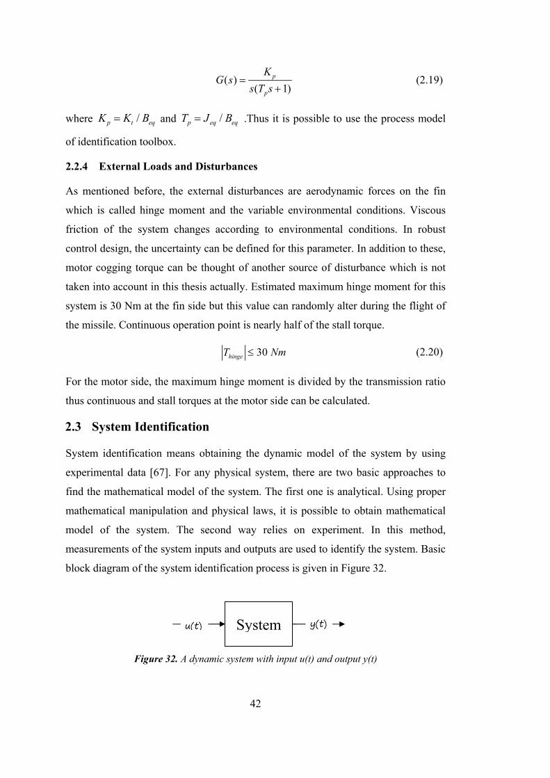
42
( )( 1)
p
p
KG s
s T s
(2.19)
where /p t eqK K B and /p eq eqT J B .Thus it is possible to use the process model
of identification toolbox.
2.2.4 External Loads and Disturbances
As mentioned before, the external disturbances are aerodynamic forces on the fin
which is called hinge moment and the variable environmental conditions. Viscous
friction of the system changes according to environmental conditions. In robust
control design, the uncertainty can be defined for this parameter. In addition to these,
motor cogging torque can be thought of another source of disturbance which is not
taken into account in this thesis actually. Estimated maximum hinge moment for this
system is 30 Nm at the fin side but this value can randomly alter during the flight of
the missile. Continuous operation point is nearly half of the stall torque.
30 hingeT Nm (2.20)
For the motor side, the maximum hinge moment is divided by the transmission ratio
thus continuous and stall torques at the motor side can be calculated.
2.3 System Identification
System identification means obtaining the dynamic model of the system by using
experimental data [67]. For any physical system, there are two basic approaches to
find the mathematical model of the system. The first one is analytical. Using proper
mathematical manipulation and physical laws, it is possible to obtain mathematical
model of the system. The second way relies on experiment. In this method,
measurements of the system inputs and outputs are used to identify the system. Basic
block diagram of the system identification process is given in Figure 32.
Figure 32. A dynamic system with input u(t) and output y(t)
System y(t) u(t)

43
Mathematical modeling and system identification approaches are compared in many
cases. In many systems, processes are so complex that it is not possible to find a
well-defined mathematical model using physical laws. In such a situation, system
identification techniques are preferred. In some cases, identification techniques can
be used to find an unknown parameters of the system that is modeled analytically
thus unknown parameters of the system are easily estimated. The obtained model by
system identification has following properties which are different than model based
on mathematics [68].
The models have limited validity because it is not possible to identify a
system exactly; therefore, engineers try to define a working range for a
certain process and then they try to identify system in this defined range.
In most cases, models have physically meaningless parameters. These
parameters are used to describe the system's overall behavior not the system
itself physically.
Construction and usage of models are quite easy.
Before starting identification procedure, one must know that identification process is
not an exact methodology thus the following important points should be taken into
account carefully [68].
For good estimations, appropriate mathematical models must be defined
firstly.
During data collection procedure, signal noises and other effects from
physical world must be taken into consideration.
All the processes may change with time depending on the working
conditions, environment etc. In order to obtain time-invariant models, these
are thought carefully.
In several applications, some signals and variables cannot be measured
properly.
Identification of a system is rather complex procedure. The identification experiment
is carried out by exciting the system using proper signals such as impulse, step,
random input etc. It is not possible to use all the signals for identification; therefore,
the input signal must be chosen carefully according to following properties.

44
The signal must be rich enough in order to guarantee that system can be
identified for intended use.
The amplitude of the input signal must be higher than noise of the output
sensor.
Another important point of system identification is determination of sampling
frequency. All the identification procedure is carried out using computer controlled
system. This causes some information loses in sampling signals. In many
applications sampling frequency must be at least 10 times higher than the bandwidth
of the system but if there is an uncertainty in the system, sampling frequency should
be selected as high as possible where the physical system permits, thus accuracy can
be maximized. Then this data can be downsampled to desired value using digital
filter and decimation [69].
Input types that can be used for system identification are given below.
Impulse: Ideally, impulse has infinitely high amplitude over zero duration. It
includes all the frequency range but it cannot be achieved practically. Thus
engineers try to obtain a very large peak during in small time interval.
Impulse signal is generally used for structure identification.
Step: One of the most commonly used signals. Signal to noise ratio in high
frequency band is low in step signal thus step signal is used to stimulus a
slow process or a slow physical system [70].
White Noise: White noise or random signal is type of a signal that whose
amplitude varies randomly. Theoretically, this signal has flat frequency
response for whole spectrum but for real, limited bandwidth systems, it is not
possible to achieve this. Important property of white noise, in a certain range,
is that it excites all the modes of the system. Generally, white noise is used to
identify electronics.
Chirp: A chirp signal is a varying frequency sinusoid. It is suitable when
frequency response within a certain range is needed.
Pseudo Random Binary Sequence (PRBS): A PRBS signal is random
sequence of rectangular pulses. Its amplitude changes between two values.
The signal sequence repeats every 2 1n values.
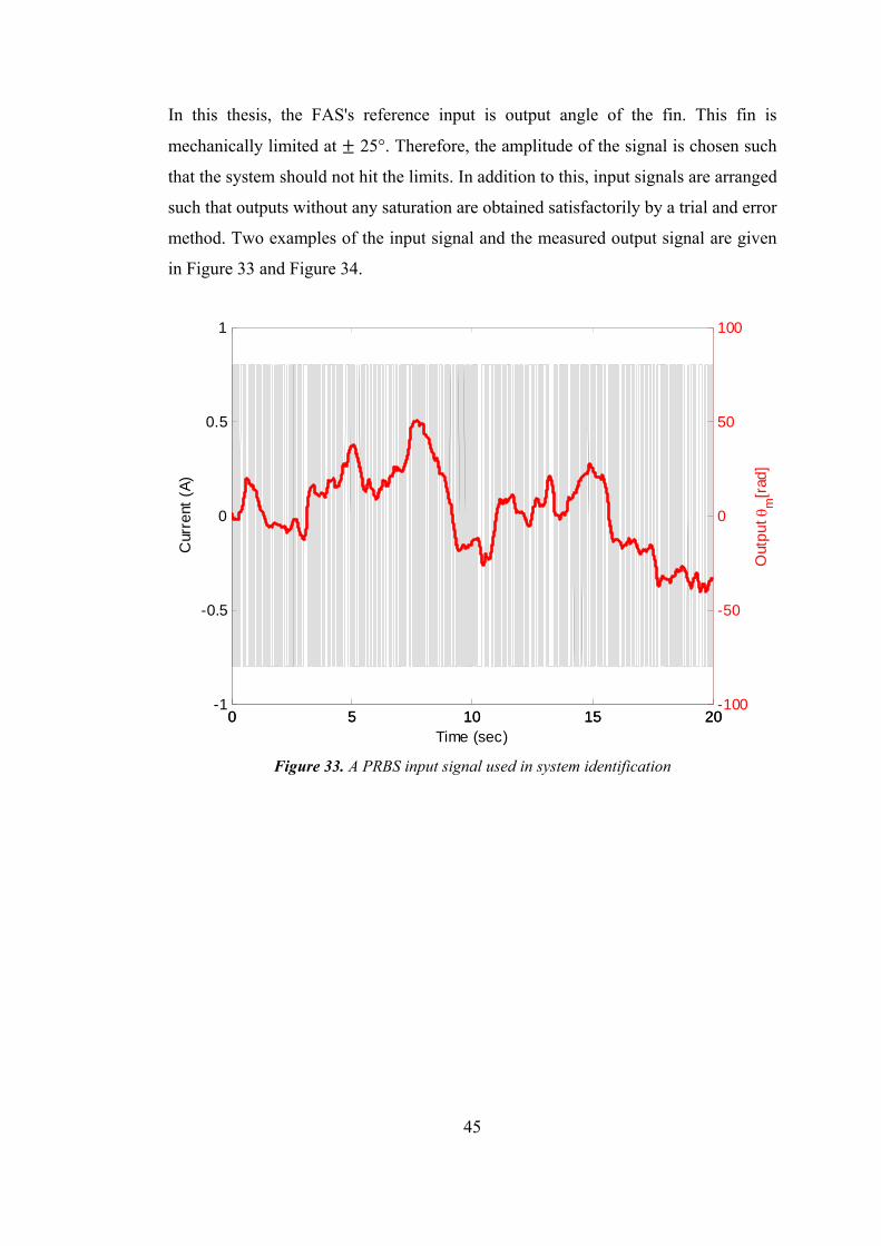
45
In this thesis, the FAS's reference input is output angle of the fin. This fin is
mechanically limited at 25°. Therefore, the amplitude of the signal is chosen such
that the system should not hit the limits. In addition to this, input signals are arranged
such that outputs without any saturation are obtained satisfactorily by a trial and error
method. Two examples of the input signal and the measured output signal are given
in Figure 33 and Figure 34.
Figure 33. A PRBS input signal used in system identification
0 5 10 15 20-1
-0.5
0
0.5
1
Cur
rent
(A
)
0 5 10 15 20-100
-50
0
50
100
Out
pu
t m
[rad
]
Time (sec)
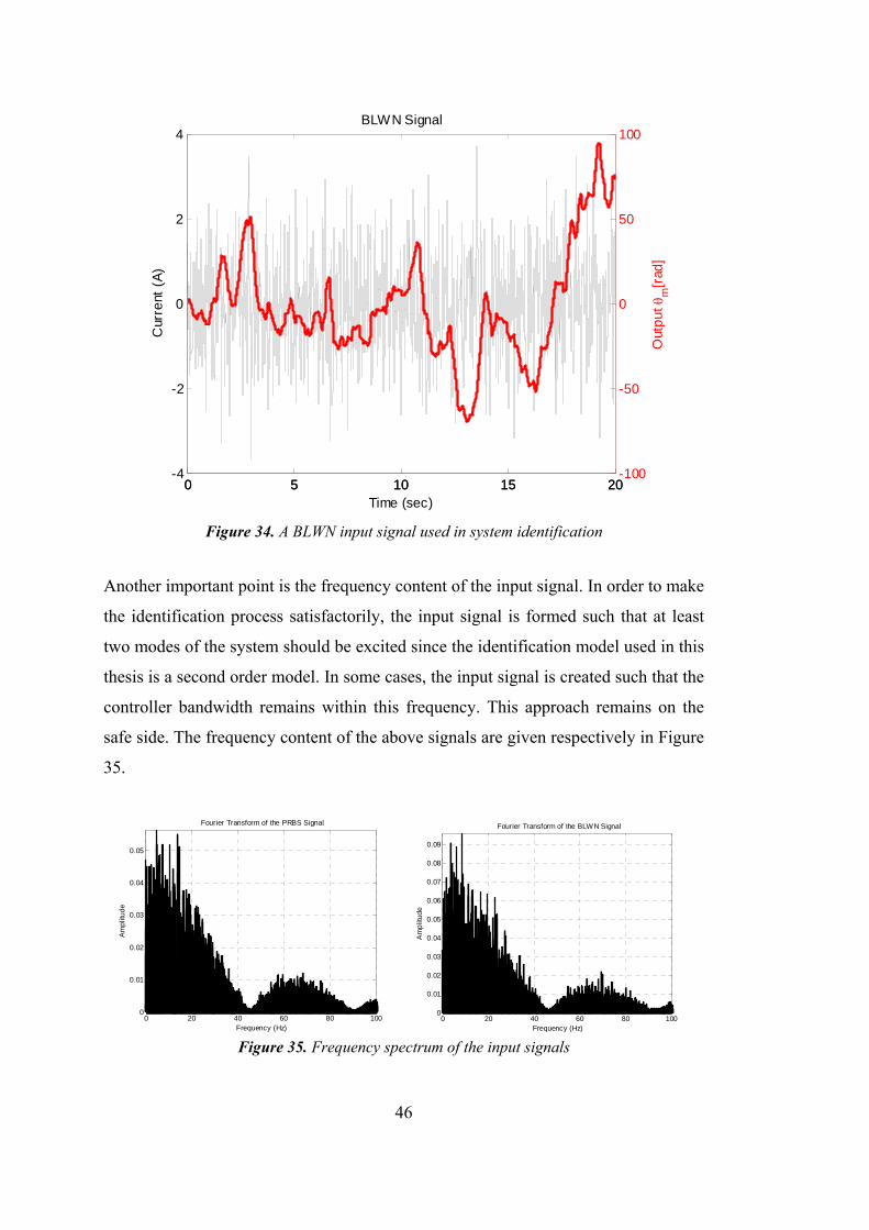
46
Figure 34. A BLWN input signal used in system identification
Another important point is the frequency content of the input signal. In order to make
the identification process satisfactorily, the input signal is formed such that at least
two modes of the system should be excited since the identification model used in this
thesis is a second order model. In some cases, the input signal is created such that the
controller bandwidth remains within this frequency. This approach remains on the
safe side. The frequency content of the above signals are given respectively in Figure
35.
Figure 35. Frequency spectrum of the input signals
0 5 10 15 20-4
-2
0
2
4
Cur
rent
(A
)
BLWN Signal
0 5 10 15 20-100
-50
0
50
100
Out
pu
t m
[rad
]
Time (sec)
0 20 40 60 80 1000
0.01
0.02
0.03
0.04
0.05
Frequency (Hz)
Am
plit
ud
e
Fourier Transform of the PRBS Signal
0 20 40 60 80 1000
0.01
0.02
0.03
0.04
0.05
0.06
0.07
0.08
0.09
Frequency (Hz)
Am
plit
ude
Fourier Transform of the BLWN Signal
47
During the system identification experiment, a MATLAB® and the real time xPC
Target® module are used in order to collect input/output signal of the system. In this
application, input signal is a current that is applied to the motor in units of Amperes
and output signal of the system is angular position of the motor measured by rotary
incremental encoder. All the input/output signal sets used to identify the mechanical
system are given in Appendix A.2. Besides, the frequency spectrum of these
input/output signal sets are also presented in Appendix A.3. In order to obtain
satisfactory results, identification procedure could be performed in two-stage. In first
stage, the system, or motor itself is tried to be identified using feasible PRBS or
BLWN signal. Then, using obtained data, model of the system could be obtained.
Using this model, new input signals could be generated in simulation environment in
order to guarantee that the outputs of the system moves within the physical limits. In
second stage, newly generated signals are applied to the system in order to identify
the system more properly. At the end of this procedure, better results could be
achieved in a short time. In this thesis, firstly the motor and the gear pair are
identified, and then the total system is identified using System Identification
ToolboxTM of MATLAB®.
System Identification ToolboxTM could be used to identify continuous or discrete
time system both in time domain and frequency domain. In this thesis, frequency
domain input-output data are preferred for identification process. Before running the
toolbox, some of preliminary preparation must be done. Firstly, all collected time
domain data must be transformed into frequency domain data. To do this, 'tfestimate'
command can be used. Then, the required frequency part of the data is filtered. For
this application, 30-40 Hz frequency band gives satisfactory results so that high
frequency modes can be neglected. Usage of toolbox is also easy. In order to use the
toolbox whose image is given in Figure 36, procedure that is given below can be
followed.
Toolbox is run using 'ident' command.
Frequency or time-domain data are imported to toolbox using import data
tab.
One of the data is chosen as validation data and the others are picked as
working data one by one.
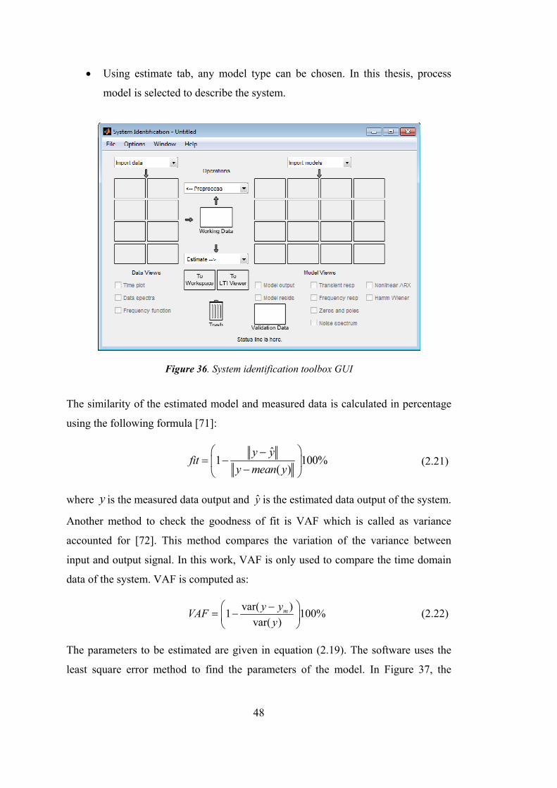
48
Using estimate tab, any model type can be chosen. In this thesis, process
model is selected to describe the system.
Figure 36. System identification toolbox GUI
The similarity of the estimated model and measured data is calculated in percentage
using the following formula [71]:
ˆ
1 100%( )
y yfit
y mean y
(2.21)
where y is the measured data output and y is the estimated data output of the system.
Another method to check the goodness of fit is VAF which is called as variance
accounted for [72]. This method compares the variation of the variance between
input and output signal. In this work, VAF is only used to compare the time domain
data of the system. VAF is computed as:
var( )
1 100%var( )
my yVAF
y
(2.22)
The parameters to be estimated are given in equation (2.19). The software uses the
least square error method to find the parameters of the model. In Figure 37, the
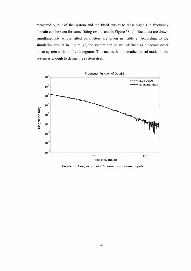
49
measured output of the system and the fitted curves to these signals in frequency
domain can be seen for some fitting results and in Figure 38, all fitted data are drawn
simultaneously whose fitted parameters are given in Table 2. According to the
simulation results in Figure 37, the system can be well-defined as a second order
linear system with one free integrator. This means that the mathematical model of the
system is enough to define the system itself.
Figure 37. Comparison of estimation results with outputs
101
102
10-4
10-3
10-2
10-1
100
101
102
103
104
Frequency (rad/s)
Frequency Function of DataB5
fitted curvemeasured data
Mag
nitu
de (
dB)
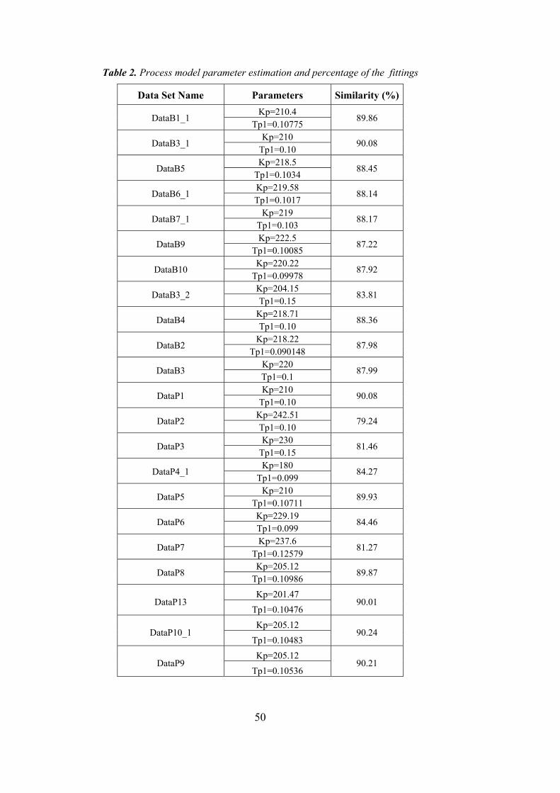
50
Table 2. Process model parameter estimation and percentage of the fittings
Data Set Name Parameters Similarity (%)
DataB1_1 Kp=210.4
89.86 Tp1=0.10775
DataB3_1 Kp=210
90.08 Tp1=0.10
DataB5 Kp=218.5
88.45 Tp1=0.1034
DataB6_1 Kp=219.58
88.14 Tp1=0.1017
DataB7_1 Kp=219
88.17 Tp1=0.103
DataB9 Kp=222.5
87.22 Tp1=0.10085
DataB10 Kp=220.22
87.92 Tp1=0.09978
DataB3_2 Kp=204.15
83.81 Tp1=0.15
DataB4 Kp=218.71
88.36 Tp1=0.10
DataB2 Kp=218.22
87.98 Tp1=0.090148
DataB3 Kp=220
87.99 Tp1=0.1
DataP1 Kp=210
90.08 Tp1=0.10
DataP2 Kp=242.51
79.24 Tp1=0.10
DataP3 Kp=230
81.46 Tp1=0.15
DataP4_1 Kp=180
84.27 Tp1=0.099
DataP5 Kp=210
89.93 Tp1=0.10711
DataP6 Kp=229.19
84.46 Tp1=0.099
DataP7 Kp=237.6
81.27 Tp1=0.12579
DataP8 Kp=205.12
89.87 Tp1=0.10986
DataP13 Kp=201.47
90.01 Tp1=0.10476
DataP10_1 Kp=205.12
90.24 Tp1=0.10483
DataP9 Kp=205.12
90.21 Tp1=0.10536
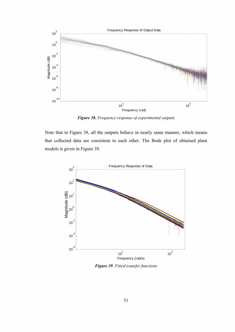
51
Figure 38. Frequency response of experimental outputs
Note that in Figure 38, all the outputs behave in nearly same manner, which means
that collected data are consistent to each other. The Bode plot of obtained plant
models is given in Figure 39.
Figure 39. Fitted transfer functions
101
102
10-10
10-8
10-6
10-4
10-2
100
102
Frequency (rad)
Mag
nitu
de
(dB
)
Frequency Response of Output Data
101
102
10-3
10-2
10-1
100
101
102
103
Frequency (rad/s)
Frequency Response of Data
Mag
nitu
de (
dB)
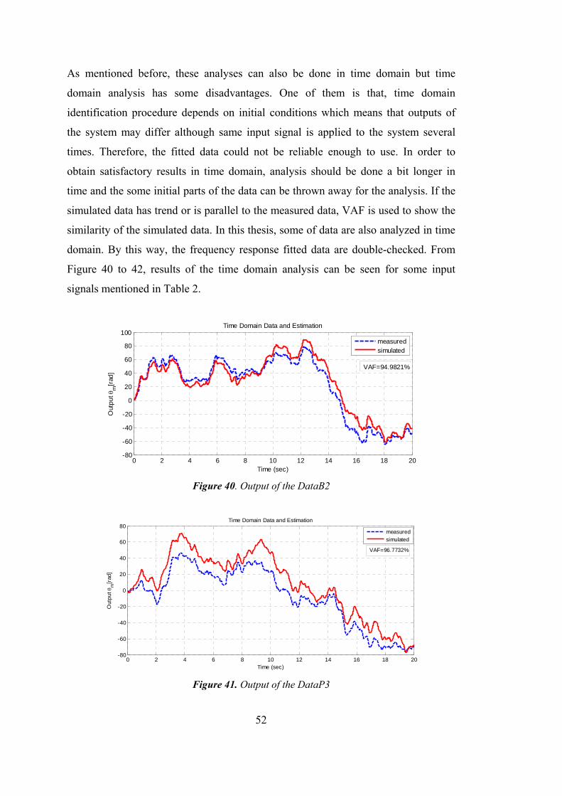
52
As mentioned before, these analyses can also be done in time domain but time
domain analysis has some disadvantages. One of them is that, time domain
identification procedure depends on initial conditions which means that outputs of
the system may differ although same input signal is applied to the system several
times. Therefore, the fitted data could not be reliable enough to use. In order to
obtain satisfactory results in time domain, analysis should be done a bit longer in
time and the some initial parts of the data can be thrown away for the analysis. If the
simulated data has trend or is parallel to the measured data, VAF is used to show the
similarity of the simulated data. In this thesis, some of data are also analyzed in time
domain. By this way, the frequency response fitted data are double-checked. From
Figure 40 to 42, results of the time domain analysis can be seen for some input
signals mentioned in Table 2.
Figure 40. Output of the DataB2
Figure 41. Output of the DataP3
0 2 4 6 8 10 12 14 16 18 20-80
-60
-40
-20
0
20
40
60
80
100
Time (sec)
Out
put
m
[rad
]
Time Domain Data and Estimation
measuredsimulated
VAF=94.9821%
0 2 4 6 8 10 12 14 16 18 20-80
-60
-40
-20
0
20
40
60
80
Time (sec)
Out
pu
t m
[rad
]
Time Domain Data and Estimation
measuredsimulated
VAF=96.7732%
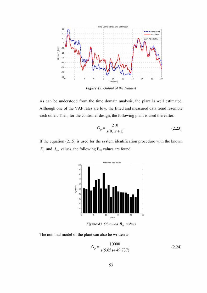
53
Figure 42. Output of the DataB4
As can be understood from the time domain analysis, the plant is well estimated.
Although one of the VAF rates are low, the fitted and measured data trend resemble
each other. Then, for the controller design, the following plant is used thereafter.
210
(0.1 1)pGs s
(2.23)
If the equation (2.15) is used for the system identification procedure with the known
tK and eqJ values, the following Beq values are found.
Figure 43. Obtained eqB values
The nominal model of the plant can also be written as
10000
(5.65s 49.737)pGs
(2.24)
0 2 4 6 8 10 12 14 16 18 20-70
-60
-50
-40
-30
-20
-10
0
10
20
30
Time (sec)
Out
pu
t m
[rad
]
Time Domain Data and Estimation
measuredsimulated
VAF 78.1942%
0 5 10 15 20 250
10
20
30
40
50
60
70
80
90
100Obtained Beq values
kg*m
m/s
Dataset

54
55
CHAPTER 3
CONTROLLER DESIGN
3.1 Requirements for the Closed Loop System
In any closed loop system, the basic requirements to be met are:
The minimum requirement should be defined to make the closed loop stable.
The controlled variable should track the command input well enough. (both
precise and fast).
Disturbance rejection should be good enough.
Finally, the closed loop system should be robust enough to deal with the
changes of system parameters in predefined degree.
As explained in previous chapters, robust control helps engineer to make such a
design especially for unknown plant variation. In this system, plant parameters have
uncertainties. Sensor noise and aerodynamic loads are the external source of
disturbances while modeling errors and environmental conditions on the plant are the
source of plant uncertainties. Apart from these, the system itself shows nonlinear
behavior. These can be grouped as saturation limit on the physical system, limited
current capacity and cogging torque of actuator. As mentioned earlier, the fin
deflection angle is limited to 25 . As might be expected, the current source is
not unlimited. The power budget of the system limits the current and for the system
in this thesis, current limit value cannot be higher than 30 A . The current limit can
cause saturation on the control signal. In addition to this, the cogging torque is
another source of disturbance. This torque always opposes to the motion of the
system. On the other hand, the angular speed of the fin is also limited.
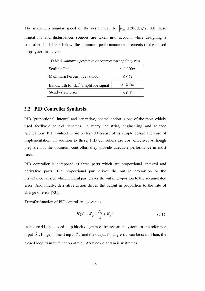
56
The maximum angular speed of the system can be 200deg/ sfin . All these
limitations and disturbances sources are taken into account while designing a
controller. In Table 3 below, the minimum performance requirements of the closed
loop system are given.
Table 3. Minimum performance requirements of the system
Settling Time 0.100s
Maximum Percent over shoot 6%
Bandwidth for 1 amplitude signal 10 Hz
Steady state error 0.1
3.2 PID Controller Synthesis
PID (proportional, integral and derivative) control action is one of the most widely
used feedback control schemes. In many industrial, engineering and science
applications, PID controllers are preferred because of its simple design and ease of
implementation. In addition to these, PID controllers are cost effective. Although
they are not the optimum controller, they provide adequate performance in most
cases.
PID controller is composed of three parts which are proportional, integral and
derivative parts. The proportional part drives the out in proportion to the
instantaneous error while integral part drives the out in proportion to the accumulated
error. And finally, derivative action drives the output in proportion to the rate of
change of error [73].
Transfer function of PID controller is given as
( ) ip d
KK s K K s
s (3.1)
In Figure 44, the closed loop block diagram of fin actuation system for the reference
input r , hinge moment input fT and the output fin angle f can be seen. Then, the
closed loop transfer function of the FAS block diagram is written as
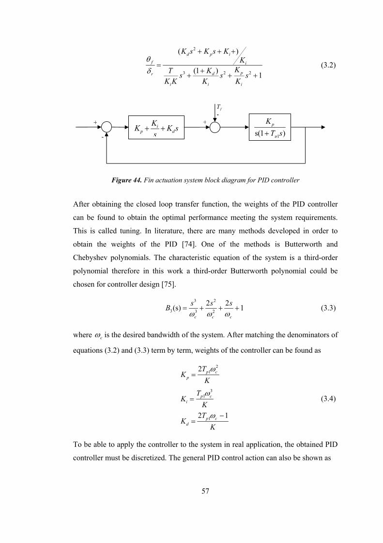
57
2
3 2 2
( )
(1 )1
d p i
f i
pdr
i i i
K s K s KK
KT Ks s s
K K K K
(3.2)
Figure 44. Fin actuation system block diagram for PID controller
After obtaining the closed loop transfer function, the weights of the PID controller
can be found to obtain the optimal performance meeting the system requirements.
This is called tuning. In literature, there are many methods developed in order to
obtain the weights of the PID [74]. One of the methods is Butterworth and
Chebyshev polynomials. The characteristic equation of the system is a third-order
polynomial therefore in this work a third-order Butterworth polynomial could be
chosen for controller design [75].
3 2
3 3 2
2 2(s) 1
c c c
s s sB
(3.3)
where c is the desired bandwidth of the system. After matching the denominators of
equations (3.2) and (3.3) term by term, weights of the controller can be found as
21
31
1
2
2 1
p cp
p ci
p cd
TK
K
TK
K
TK
K
(3.4)
To be able to apply the controller to the system in real application, the obtained PID
controller must be discretized. The general PID control action can also be shown as
fT
+i
p d
KK K s
s
-
+-
1s(1 )p
p
K
T s
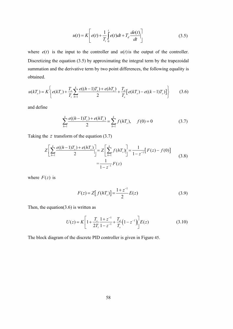
58
0
1 ( )( ) ( ) ( )
t
di
de tu t K e t e t dt T
T dt
(3.5)
where ( )e t is the input to the controller and ( )u t is the output of the controller.
Discretizing the equation (3.5) by approximating the integral term by the trapezoidal
summation and the derivative term by two point differences, the following equality is
obtained.
1
(( 1) ) ( )( ) ( ) ( ) (( 1) )
2
ks s s d
s s s shi s
T e h T e hT Tu kT K e kT e kT e k T
T T
(3.6)
and define
1 1
(( 1) ) ( )( ), (0) 0
2
k ks s
sh h
e h T e hTf hT f
(3.7)
Taking the z transform of the equation (3.7)
1
1 1
1
(( 1) ) ( ) 1( ) ( ) (0)
2 1
1 = ( )
1
k ks s
sh h
e h T e hTZ Z f hT F z f
z
F zz
(3.8)
where ( )F z is
11
( ) ( ) ( )2s
zF z Z f hT E z
(3.9)
Then, the equation(3.6) is written as
1
11
1( ) 1 1 ( )
2 1s d
i s
T z TU z K z E z
T z T
(3.10)
The block diagram of the discrete PID controller is given in Figure 45.
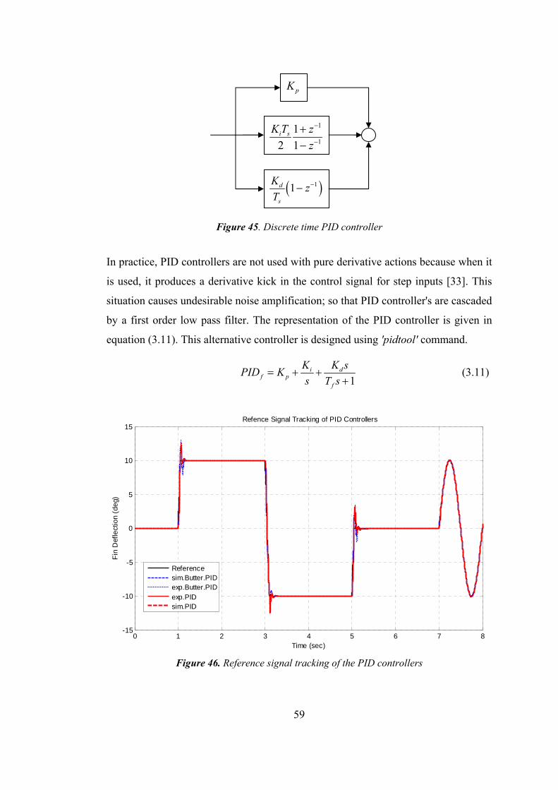
59
Figure 45. Discrete time PID controller
In practice, PID controllers are not used with pure derivative actions because when it
is used, it produces a derivative kick in the control signal for step inputs [33]. This
situation causes undesirable noise amplification; so that PID controller's are cascaded
by a first order low pass filter. The representation of the PID controller is given in
equation (3.11). This alternative controller is designed using 'pidtool' command.
1
i df p
f
K K sPID K
s T s
(3.11)
Figure 46. Reference signal tracking of the PID controllers
0 1 2 3 4 5 6 7 8-15
-10
-5
0
5
10
15Refence Signal Tracking of PID Controllers
Time (sec)
Fin
Def
lect
ion
(de
g)
Referencesim.Butter.PIDexp.Butter.PIDexp.PIDsim.PID
pK
11d
s
Kz
T
1
1
1
2 1i sK T z
z
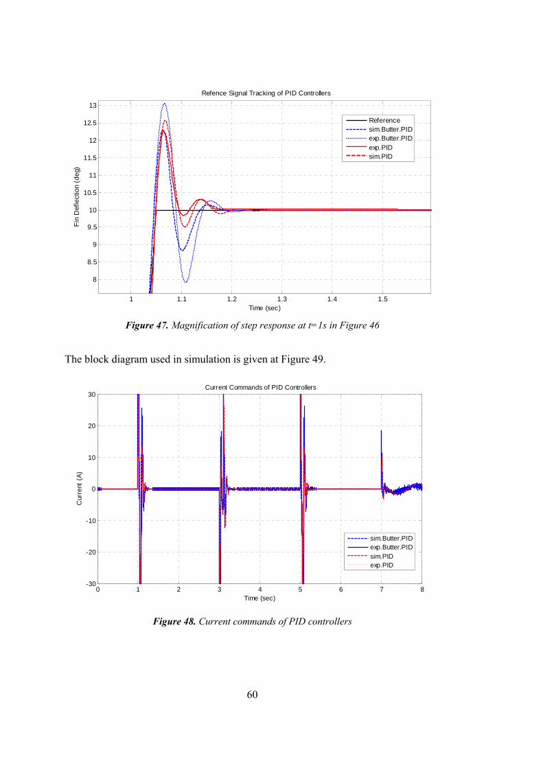
60
Figure 47. Magnification of step response at t=1s in Figure 46
The block diagram used in simulation is given at Figure 49.
Figure 48. Current commands of PID controllers
1 1.1 1.2 1.3 1.4 1.5
8
8.5
9
9.5
10
10.5
11
11.5
12
12.5
13
Refence Signal Tracking of PID Controllers
Time (sec)
Fin
Def
lect
ion
(d
eg)
Referencesim.Butter.PIDexp.Butter.PIDexp.PIDsim.PID
0 1 2 3 4 5 6 7 8-30
-20
-10
0
10
20
30Current Commands of PID Controllers
Time (sec)
Cur
rent
(A
)
sim.Butter.PIDexp.Butter.PIDsim.PIDexp.PID
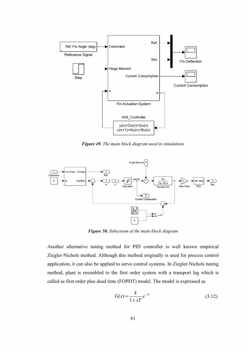
61
Figure 49. The main block diagram used in simulations
Figure 50. Subsystem of the main block diagram
Another alternative tuning method for PID controller is well known empirical
Ziegler-Nichols method. Although this method originally is used for process control
application, it can also be applied to servo control systems. In Ziegler-Nichols tuning
method, plant is resembled to the first order system with a transport lag which is
called as first order plus dead time (FOPDT) model. The model is expressed as
( )1
sLkG s e
sT
(3.12)
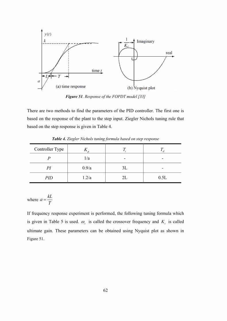
62
Figure 51. Response of the FOPDT model [33]
There are two methods to find the parameters of the PID controller. The first one is
based on the response of the plant to the step input. Ziegler Nichols tuning rule that
based on the step response is given in Table 4.
Table 4. Ziegler Nichols tuning formula based on step response
Controller Type pK iT dT
P 1/a - -
PI 0.9/a 3L -
PID 1.2/a 2L 0.5L
where kL
aT
If frequency response experiment is performed, the following tuning formula which
is given in Table 5 is used. c is called the crossover frequency and cK is called
ultimate gain. These parameters can be obtained using Nyquist plot as shown in
Figure 51.
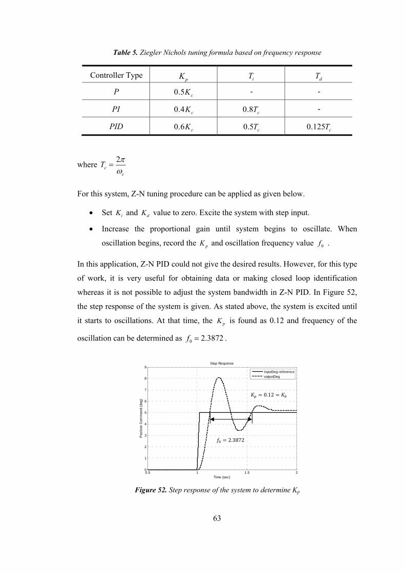
63
Table 5. Ziegler Nichols tuning formula based on frequency response
Controller Type pK iT dT
P 0.5 cK - -
PI 0.4 cK 0.8 cT -
PID 0.6 cK 0.5 cT 0.125 cT
where 2
cc
T
For this system, Z-N tuning procedure can be applied as given below.
Set iK and dK value to zero. Excite the system with step input.
Increase the proportional gain until system begins to oscillate. When
oscillation begins, record the pK and oscillation frequency value 0f .
In this application, Z-N PID could not give the desired results. However, for this type
of work, it is very useful for obtaining data or making closed loop identification
whereas it is not possible to adjust the system bandwidth in Z-N PID. In Figure 52,
the step response of the system is given. As stated above, the system is excited until
it starts to oscillations. At that time, the pK is found as 0.12 and frequency of the
oscillation can be determined as 0 2.3872f .
Figure 52. Step response of the system to determine Kp
0.5 1 1.5 20
1
2
3
4
5
6
7
8
9
Time (sec)
Pos
itio
n C
om
ma
nd
(deg
)
Step Response
inputDeg-referenceoutputDeg
0.12
2.3872
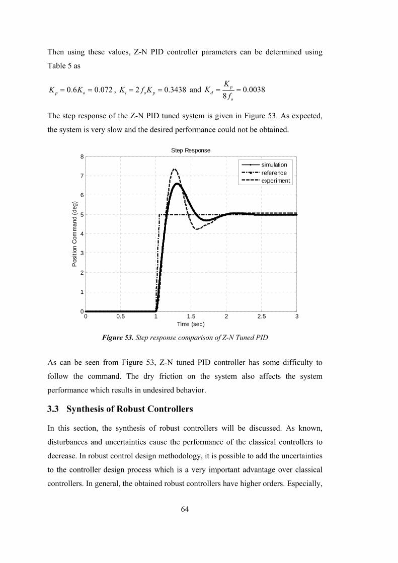
64
Then using these values, Z-N PID controller parameters can be determined using
Table 5 as
0.6 0.072p oK K , 2 0.3438i o pK f K and 0.00388
pd
o
KK
f
The step response of the Z-N PID tuned system is given in Figure 53. As expected,
the system is very slow and the desired performance could not be obtained.
Figure 53. Step response comparison of Z-N Tuned PID
As can be seen from Figure 53, Z-N tuned PID controller has some difficulty to
follow the command. The dry friction on the system also affects the system
performance which results in undesired behavior.
3.3 Synthesis of Robust Controllers
In this section, the synthesis of robust controllers will be discussed. As known,
disturbances and uncertainties cause the performance of the classical controllers to
decrease. In robust control design methodology, it is possible to add the uncertainties
to the controller design process which is a very important advantage over classical
controllers. In general, the obtained robust controllers have higher orders. Especially,
0 0.5 1 1.5 2 2.5 30
1
2
3
4
5
6
7
8Step Response
Time (sec)
Pos
itio
n C
omm
an
d (d
eg)
simulationreferenceexperiment

65
apart from the plant, the weighting functions selection affects the order of controller;
therefore, in order to keep the controller order lower, first order weighing functions
are generally chosen. If the obtained controller order is too high for computational
cost, it is possible to decrease the order of controller using some order-reducing
algorithms; however, the powerful calculation tools, high speed microprocessor
currently make it easy to develop such controllers.
The aim of the robust controller design is same as in classical controllers; however
the main difference is that the robust controllers maintain the stability and
performance under the pre-specified uncertainties and disturbances. In this thesis, the
proper system model and the desired controller are obtained using MATLAB®
"hinfsyn" command.
The block diagrams for the controller synthesis and the input-output signals to the
system are given in Figure 54-57. The parameters defining uncertainties,
disturbances, weighting and cost functions are defined as follows:
refW : Weighting function for reference signal
hingeW : Weighting function for external aerodynamic loads
uW : Cost function for controller output
idealW : Ideal closed loop system
perfW : Cost function for performance index
noiseW : Weighting function for sensor noise
mW : Model uncertainty function
N : Transmission ratio for mechanism
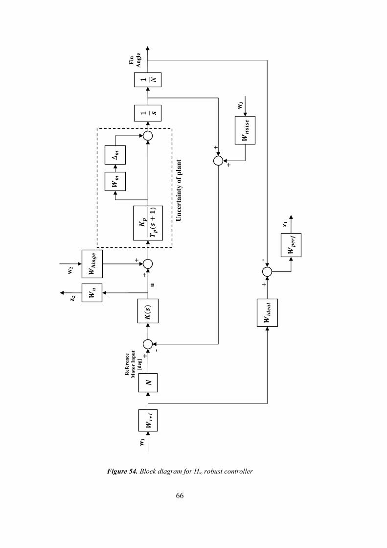
66
Figure 54. Block diagram for H∞ robust controller
w2
Un
cert
ain
ty o
f p
lan
t
1
Ref
eren
ce
Mot
or I
np
ut
[deg
] 1
z 2
+ -
+
+
+
Fin
A
ngl
e
∆
z 1
-
+
+
w1
w3
u
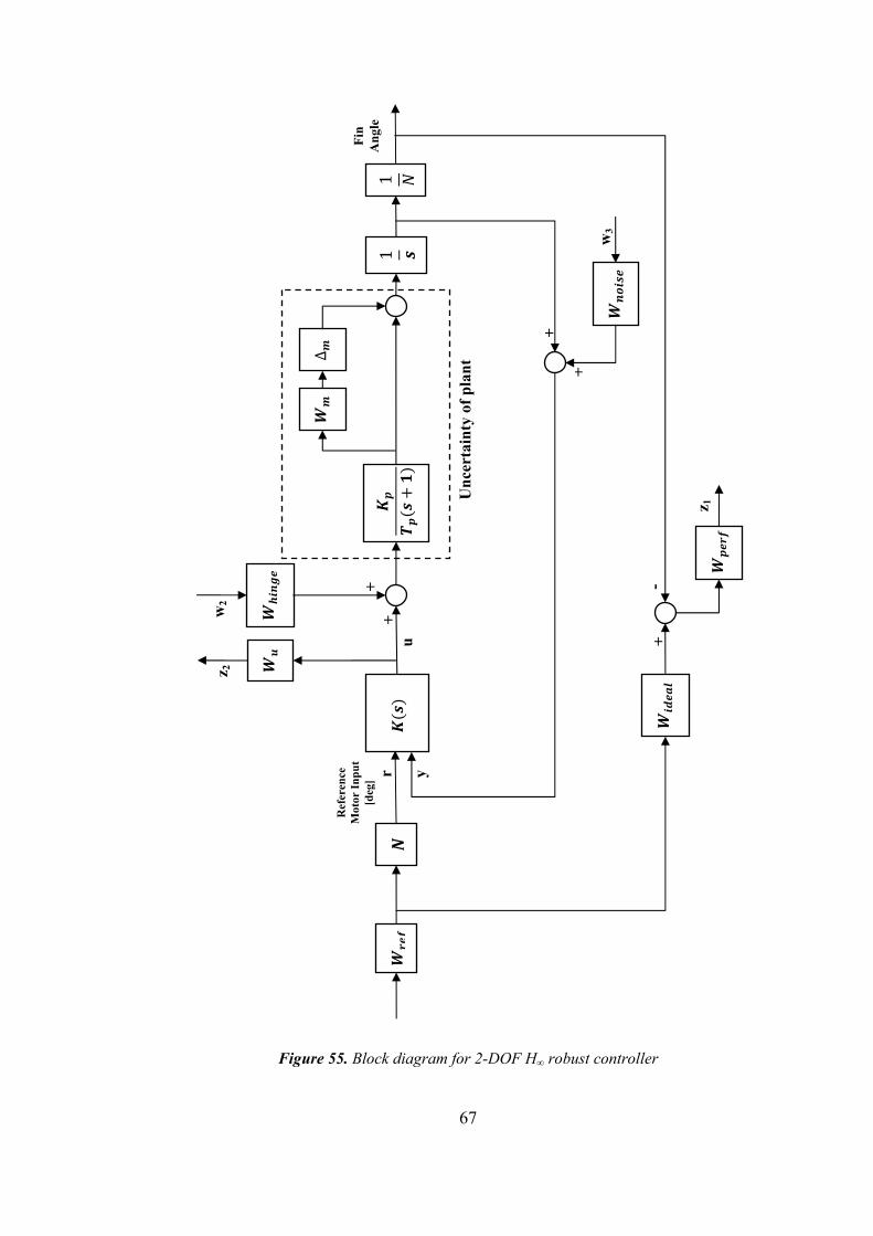
67
Figure 55. Block diagram for 2-DOF H∞ robust controller
w2
Un
cert
ain
ty o
f p
lan
t
1
Ref
eren
ce
Mot
or I
np
ut
[deg
]
1
z 2
+
+
+
Fin
A
ngl
e
∆
z 1
-
+
+
r y
w3
u
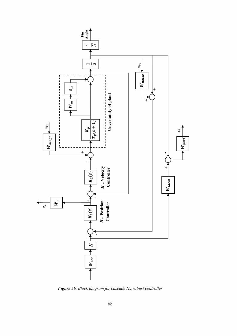
68
Figure 56. Block diagram for cascade H∞ robust controller
Fin
A
ngl
e
w
2
Un
cert
ain
ty o
f p
lan
t
1
1
z 2
+ -
+
+
+
∆
z 1
-
+
+
w3
+
-
Pos
itio
n
Con
trol
ler
Vel
ocit
y C
ontr
olle
r
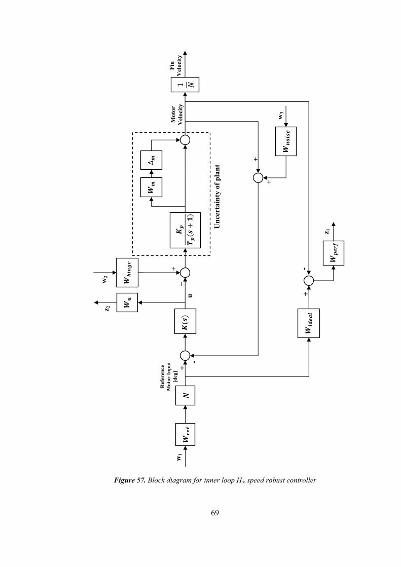
69
Figure 57. Block diagram for inner loop H∞ speed robust controller
w2
Un
cert
ain
ty o
f p
lan
t
Ref
eren
ce
Mot
or I
np
ut
[deg
] 1
z 2
+ -
+
+
+
Fin
V
eloc
ity
∆
z 1
-
+
+
w1
w3
Mot
or
Vel
ocit
y
u
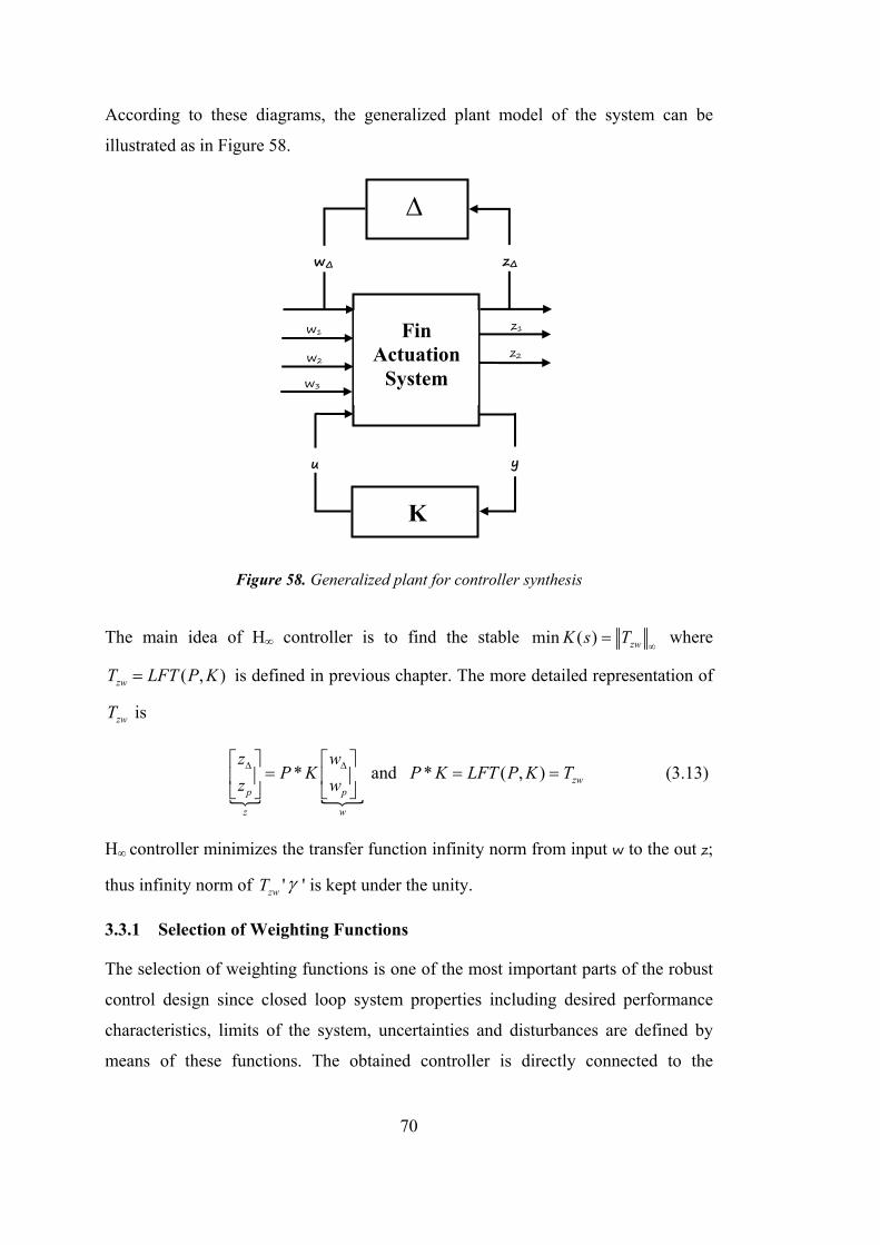
70
According to these diagrams, the generalized plant model of the system can be
illustrated as in Figure 58.
Figure 58. Generalized plant for controller synthesis
The main idea of H∞ controller is to find the stable min ( ) zwK s T
where
( , )zwT LFT P K is defined in previous chapter. The more detailed representation of
zwT is
* and * ( , ) zwp p
z w
z wP K P K LFT P K T
z w
(3.13)
H∞ controller minimizes the transfer function infinity norm from input w to the out z;
thus infinity norm of zwT ' ' is kept under the unity.
3.3.1 Selection of Weighting Functions
The selection of weighting functions is one of the most important parts of the robust
control design since closed loop system properties including desired performance
characteristics, limits of the system, uncertainties and disturbances are defined by
means of these functions. The obtained controller is directly connected to the
z2
w3
w2
w1 z1
Fin Actuation
System
K
u y
wΔ zΔ
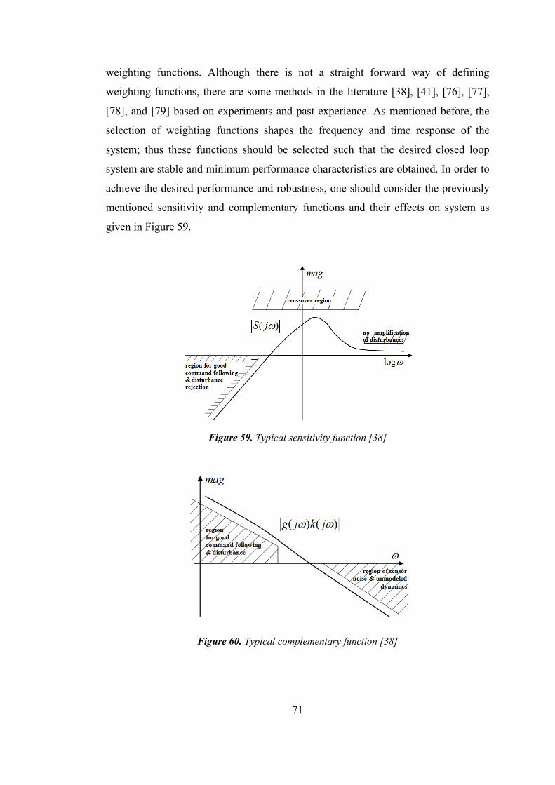
71
weighting functions. Although there is not a straight forward way of defining
weighting functions, there are some methods in the literature [38], [41], [76], [77],
[78], and [79] based on experiments and past experience. As mentioned before, the
selection of weighting functions shapes the frequency and time response of the
system; thus these functions should be selected such that the desired closed loop
system are stable and minimum performance characteristics are obtained. In order to
achieve the desired performance and robustness, one should consider the previously
mentioned sensitivity and complementary functions and their effects on system as
given in Figure 59.
Figure 59. Typical sensitivity function [38]
Figure 60. Typical complementary function [38]
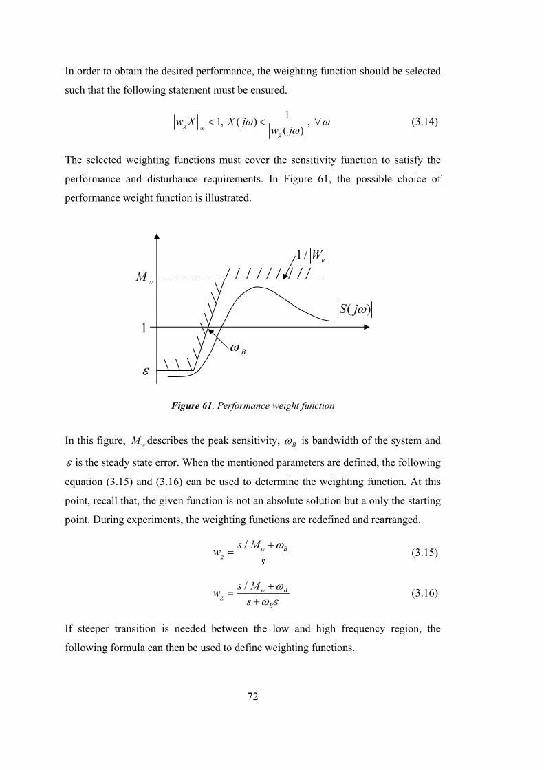
72
In order to obtain the desired performance, the weighting function should be selected
such that the following statement must be ensured.
1
1, ( ) , ( )
g
g
w X X jw j
(3.14)
The selected weighting functions must cover the sensitivity function to satisfy the
performance and disturbance requirements. In Figure 61, the possible choice of
performance weight function is illustrated.
Figure 61. Performance weight function
In this figure, wM describes the peak sensitivity, B is bandwidth of the system and
is the steady state error. When the mentioned parameters are defined, the following
equation (3.15) and (3.16) can be used to determine the weighting function. At this
point, recall that, the given function is not an absolute solution but a only the starting
point. During experiments, the weighting functions are redefined and rearranged.
/ w B
g
s Mw
s
(3.15)
/ w B
gB
s Mw
s
(3.16)
If steeper transition is needed between the low and high frequency region, the
following formula can then be used to define weighting functions.
( )S j
1/ eW
1
B
wM
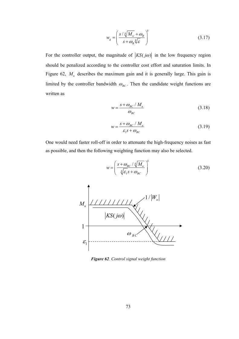
73
/
kk
w Bg k
B
s Mw
s
(3.17)
For the controller output, the magnitude of ( )KS j in the low frequency region
should be penalized according to the controller cost effort and saturation limits. In
Figure 62, uM describes the maximum gain and it is generally large. This gain is
limited by the controller bandwidth BC . Then the candidate weight functions are
written as
/BC u
BC
s Mw
(3.18)
1
/BC u
BC
s Mw
s
(3.19)
One would need faster roll-off in order to attenuate the high-frequency noises as fast
as possible, and then the following weighting function may also be selected.
1
/k
kBC u
kBC
s Mw
s
(3.20)
Figure 62. Control signal weight function
( )KS j
1 / uW
1
1B C
uM
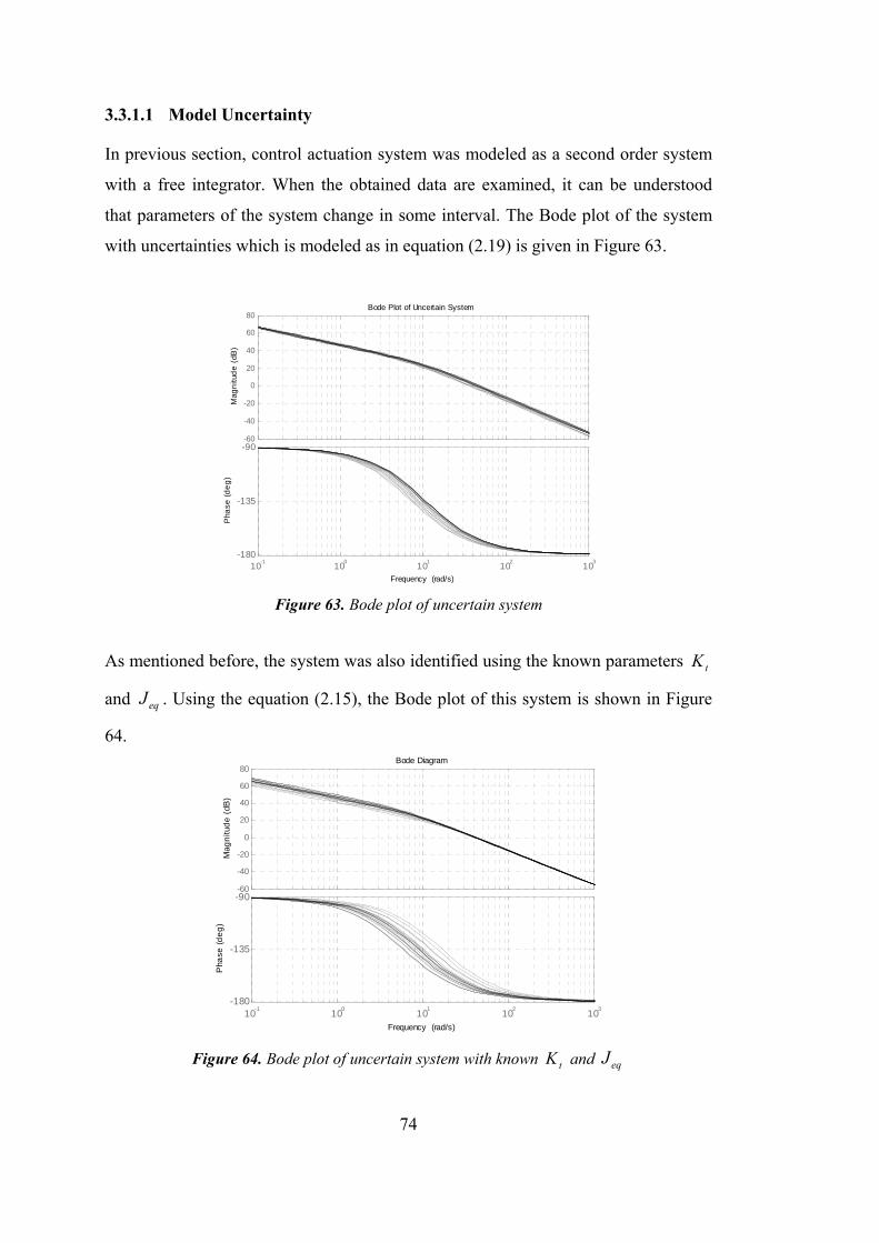
74
3.3.1.1 Model Uncertainty
In previous section, control actuation system was modeled as a second order system
with a free integrator. When the obtained data are examined, it can be understood
that parameters of the system change in some interval. The Bode plot of the system
with uncertainties which is modeled as in equation (2.19) is given in Figure 63.
Figure 63. Bode plot of uncertain system
As mentioned before, the system was also identified using the known parameters tK
and eqJ . Using the equation (2.15), the Bode plot of this system is shown in Figure
64.
Figure 64. Bode plot of uncertain system with known tK and eqJ
-60
-40
-20
0
20
40
60
80
Mag
nitu
de
(dB
)
10-1
100
101
102
103
-180
-135
-90
Pha
se (
de
g)
Bode Plot of Uncertain System
Frequency (rad/s)
-60
-40
-20
0
20
40
60
80
Mag
nitu
de
(dB
)
10-1
100
101
102
103
-180
-135
-90
Pha
se (
de
g)
Bode Diagram
Frequency (rad/s)
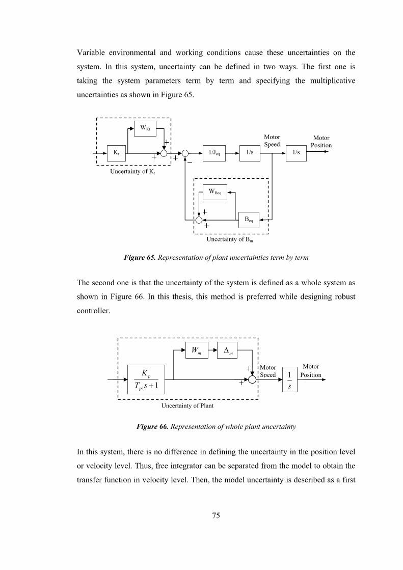
75
Variable environmental and working conditions cause these uncertainties on the
system. In this system, uncertainty can be defined in two ways. The first one is
taking the system parameters term by term and specifying the multiplicative
uncertainties as shown in Figure 65.
Figure 65. Representation of plant uncertainties term by term
The second one is that the uncertainty of the system is defined as a whole system as
shown in Figure 66. In this thesis, this method is preferred while designing robust
controller.
Figure 66. Representation of whole plant uncertainty
In this system, there is no difference in defining the uncertainty in the position level
or velocity level. Thus, free integrator can be separated from the model to obtain the
transfer function in velocity level. Then, the model uncertainty is described as a first
Uncertainty of Plant
1 1p
p
K
T s 1
s
mW
MotorSpeed
Motor Position
m
Kt 1/Jeq 1/s 1/s
Motor Speed
Motor Position
Beq
WBeq
WKt
Uncertainty of Kt
Uncertainty of Bm
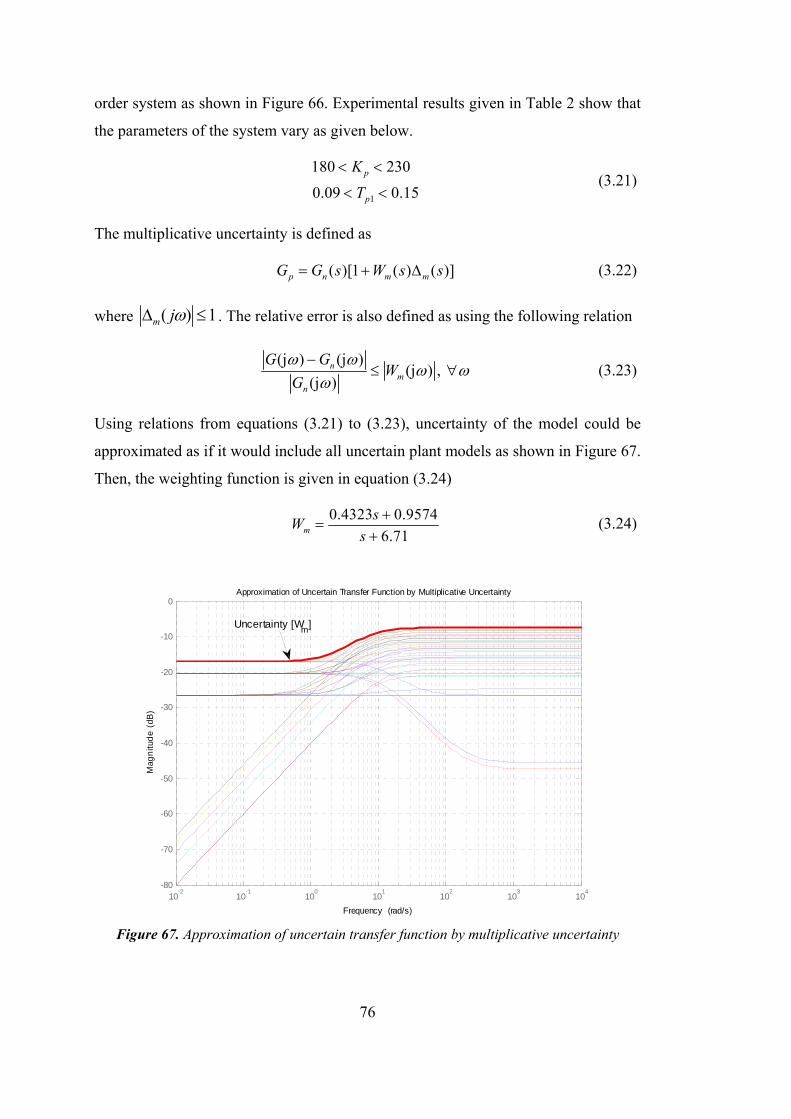
76
order system as shown in Figure 66. Experimental results given in Table 2 show that
the parameters of the system vary as given below.
1
180 230
0.09 0.15
p
p
K
T
(3.21)
The multiplicative uncertainty is defined as
( )[1 ( ) ( )]p n m mG G s W s s (3.22)
where ( ) 1m j . The relative error is also defined as using the following relation
(j ) (j )
(j ) , (j )
nm
n
G GW
G
(3.23)
Using relations from equations (3.21) to (3.23), uncertainty of the model could be
approximated as if it would include all uncertain plant models as shown in Figure 67.
Then, the weighting function is given in equation (3.24)
0.4323 0.9574
6.71m
sW
s
(3.24)
Figure 67. Approximation of uncertain transfer function by multiplicative uncertainty
10-2
10-1
100
101
102
103
104
-80
-70
-60
-50
-40
-30
-20
-10
0
Mag
nitu
de
(dB
)
Uncertainty [Wm
]
Approximation of Uncertain Transfer Function by Multiplicative Uncertainty
Frequency (rad/s)
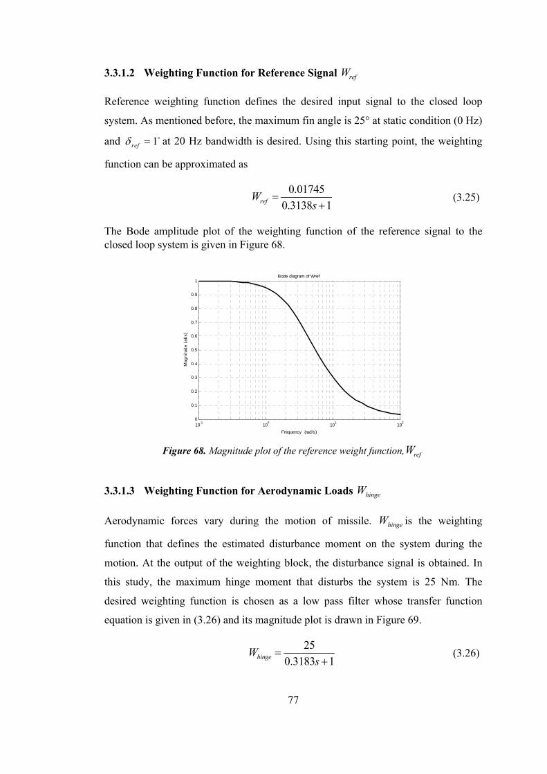
77
3.3.1.2 Weighting Function for Reference Signal refW
Reference weighting function defines the desired input signal to the closed loop
system. As mentioned before, the maximum fin angle is 25° at static condition (0 Hz)
and 1ref at 20 Hz bandwidth is desired. Using this starting point, the weighting
function can be approximated as
0.01745
0.3138 1refWs
(3.25)
The Bode amplitude plot of the weighting function of the reference signal to the closed loop system is given in Figure 68.
Figure 68. Magnitude plot of the reference weight function, refW
3.3.1.3 Weighting Function for Aerodynamic Loads hingeW
Aerodynamic forces vary during the motion of missile. hingeW is the weighting
function that defines the estimated disturbance moment on the system during the
motion. At the output of the weighting block, the disturbance signal is obtained. In
this study, the maximum hinge moment that disturbs the system is 25 Nm. The
desired weighting function is chosen as a low pass filter whose transfer function
equation is given in (3.26) and its magnitude plot is drawn in Figure 69.
25
0.3183 1hingeWs
(3.26)
10-1
100
101
102
0
0.1
0.2
0.3
0.4
0.5
0.6
0.7
0.8
0.9
1
Mag
nitu
de
(ab
s)
Bode diagram of Wref
Frequency (rad/s)
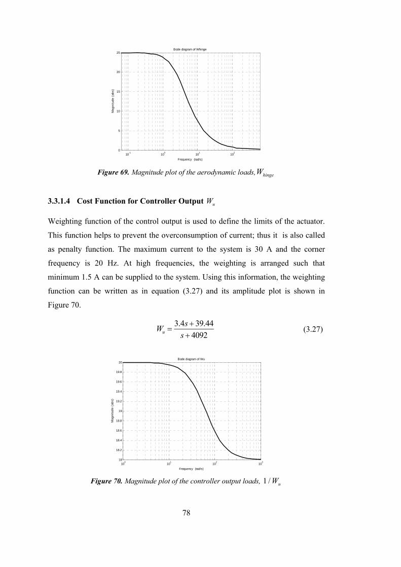
78
Figure 69. Magnitude plot of the aerodynamic loads, hingeW
3.3.1.4 Cost Function for Controller Output uW
Weighting function of the control output is used to define the limits of the actuator.
This function helps to prevent the overconsumption of current; thus it is also called
as penalty function. The maximum current to the system is 30 A and the corner
frequency is 20 Hz. At high frequencies, the weighting is arranged such that
minimum 1.5 A can be supplied to the system. Using this information, the weighting
function can be written as in equation (3.27) and its amplitude plot is shown in
Figure 70.
3.4 39.44
4092u
sW
s
(3.27)
Figure 70. Magnitude plot of the controller output loads, 1 / uW
10-1
100
101
102
0
5
10
15
20
25
Mag
nitu
de
(ab
s)
Bode diagram of Whinge
Frequency (rad/s)
100
101
102
103
18
18.2
18.4
18.6
18.8
19
19.2
19.4
19.6
19.8
20
Mag
nitu
de
(ab
s)
Bode diagram of Wu
Frequency (rad/s)
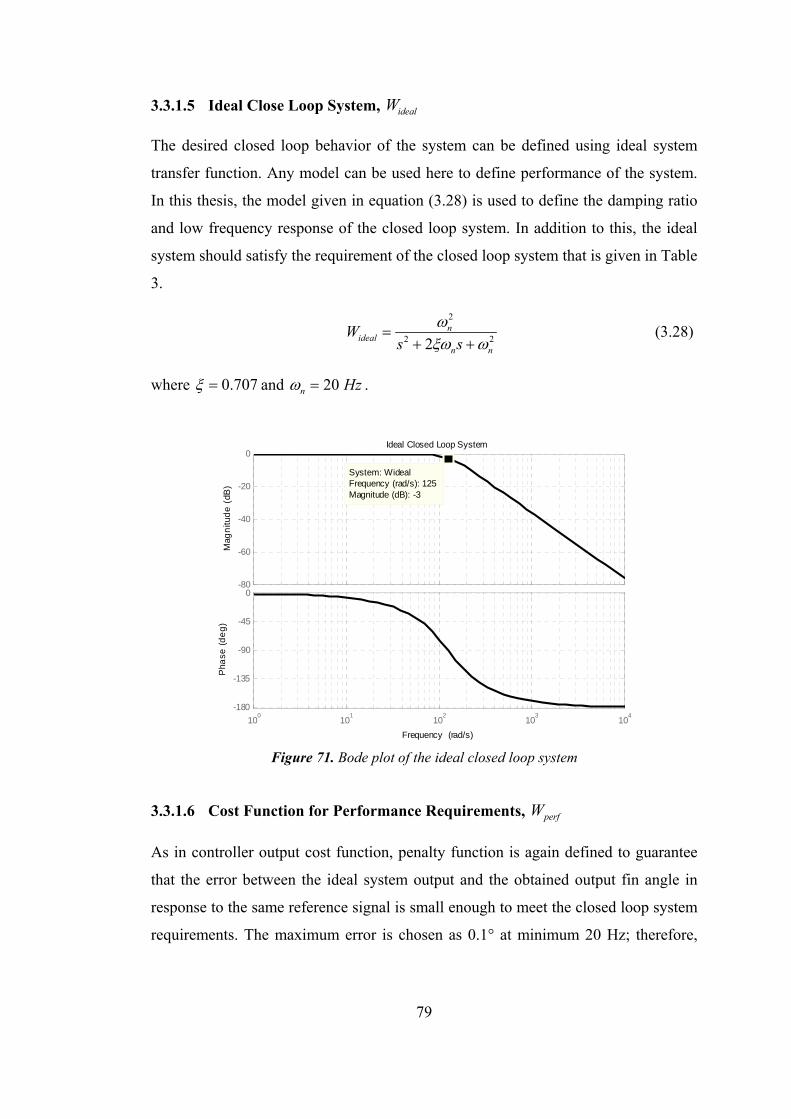
79
3.3.1.5 Ideal Close Loop System, idealW
The desired closed loop behavior of the system can be defined using ideal system
transfer function. Any model can be used here to define performance of the system.
In this thesis, the model given in equation (3.28) is used to define the damping ratio
and low frequency response of the closed loop system. In addition to this, the ideal
system should satisfy the requirement of the closed loop system that is given in Table
3.
2
2 22n
idealn n
Ws s
(3.28)
where 0.707 and 20 n Hz .
Figure 71. Bode plot of the ideal closed loop system
3.3.1.6 Cost Function for Performance Requirements, perfW
As in controller output cost function, penalty function is again defined to guarantee
that the error between the ideal system output and the obtained output fin angle in
response to the same reference signal is small enough to meet the closed loop system
requirements. The maximum error is chosen as 0.1° at minimum 20 Hz; therefore,
100
101
102
103
104
-180
-135
-90
-45
0
Pha
se (
de
g)
Ideal Closed Loop System
Frequency (rad/s)
-80
-60
-40
-20
0
System: WidealFrequency (rad/s): 125Magnitude (dB): -3
Mag
nitu
de
(dB
)
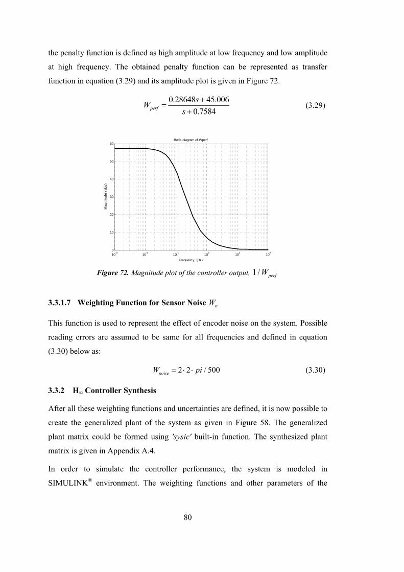
80
the penalty function is defined as high amplitude at low frequency and low amplitude
at high frequency. The obtained penalty function can be represented as transfer
function in equation (3.29) and its amplitude plot is given in Figure 72.
0.28648 45.006
0.7584perf
sW
s
(3.29)
Figure 72. Magnitude plot of the controller output, 1 / perfW
3.3.1.7 Weighting Function for Sensor Noise nW
This function is used to represent the effect of encoder noise on the system. Possible
reading errors are assumed to be same for all frequencies and defined in equation
(3.30) below as:
2 2 / 500noiseW pi (3.30)
3.3.2 H∞ Controller Synthesis
After all these weighting functions and uncertainties are defined, it is now possible to
create the generalized plant of the system as given in Figure 58. The generalized
plant matrix could be formed using 'sysic' built-in function. The synthesized plant
matrix is given in Appendix A.4.
In order to simulate the controller performance, the system is modeled in
SIMULINK® environment. The weighting functions and other parameters of the
10-3
10-2
10-1
100
101
102
0
10
20
30
40
50
60
Mag
nitu
de
(ab
s)
Bode diagram of Wperf
Frequency (Hz)
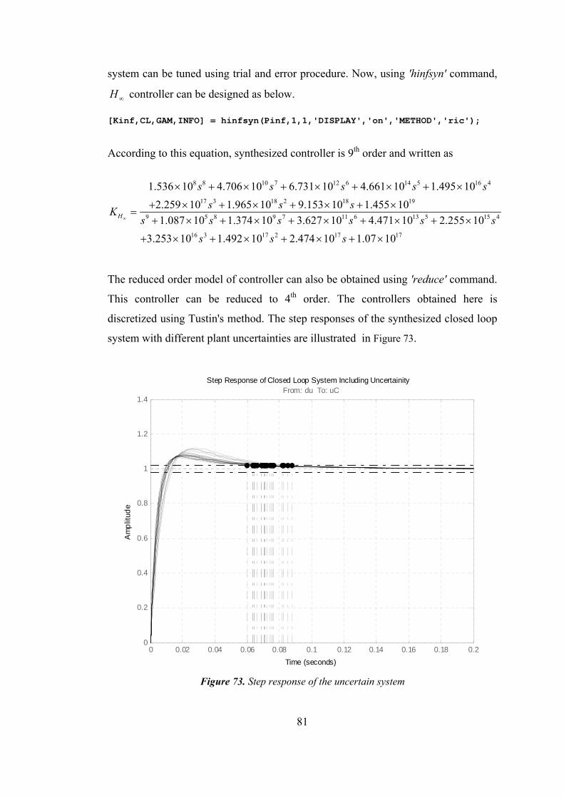
81
system can be tuned using trial and error procedure. Now, using 'hinfsyn' command,
H controller can be designed as below.
[Kinf,CL,GAM,INFO] = hinfsyn(Pinf,1,1,'DISPLAY','on','METHOD','ric');
According to this equation, synthesized controller is 9th order and written as
8 8 10 7 12 6 14 5 16 4
17 3 18 2 18 19
9 5 8 9 7 11 6 13 5 15 4
16 3
1.536 10 4.706 10 6.731 10 4.661 10 1.495 10
2.259 10 1.965 10 9.153 10 1.455 10
1.087 10 1.374 10 3.627 10 4.471 10 2.255 10
3.253 10 1.492
H
s s s s s
s s sK
s s s s s s
s
17 2 17 1710 2.474 10 1.07 10s s
The reduced order model of controller can also be obtained using 'reduce' command.
This controller can be reduced to 4th order. The controllers obtained here is
discretized using Tustin's method. The step responses of the synthesized closed loop
system with different plant uncertainties are illustrated in Figure 73.
Figure 73. Step response of the uncertain system
0 0.02 0.04 0.06 0.08 0.1 0.12 0.14 0.16 0.18 0.20
0.2
0.4
0.6
0.8
1
1.2
1.4From: du To: uC
Step Response of Closed Loop System Including Uncertainity
Time (seconds)
Am
plit
ude
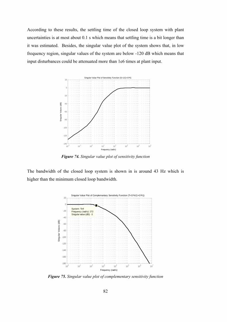
82
According to these results, the settling time of the closed loop system with plant
uncertainties is at most about 0.1 s which means that settling time is a bit longer than
it was estimated. Besides, the singular value plot of the system shows that, in low
frequency region, singular values of the system are below -120 dB which means that
input disturbances could be attenuated more than 1e6 times at plant input.
Figure 74. Singular value plot of sensitivity function
The bandwidth of the closed loop system is shown in is around 43 Hz which is
higher than the minimum closed loop bandwidth.
Figure 75. Singular value plot of complementary sensitivity function
10-2
10-1
100
101
102
103
104
105
-140
-120
-100
-80
-60
-40
-20
0
20Singular Value Plot of Sensitivity Function (S=1/(1+G*K)
Frequency (rad/s)
Sin
gu
lar
Va
lue
s (d
B)
100
101
102
103
104
105
106
107
-180
-160
-140
-120
-100
-80
-60
-40
-20
0
20
System: TinfFrequency (rad/s): 272Singular value (dB): -3
Singular Value Plot of Complemantary Sensitivity Function (T=G*K/(1+G*K))
Frequency (rad/s)
Sin
gu
lar
Va
lue
s (d
B)
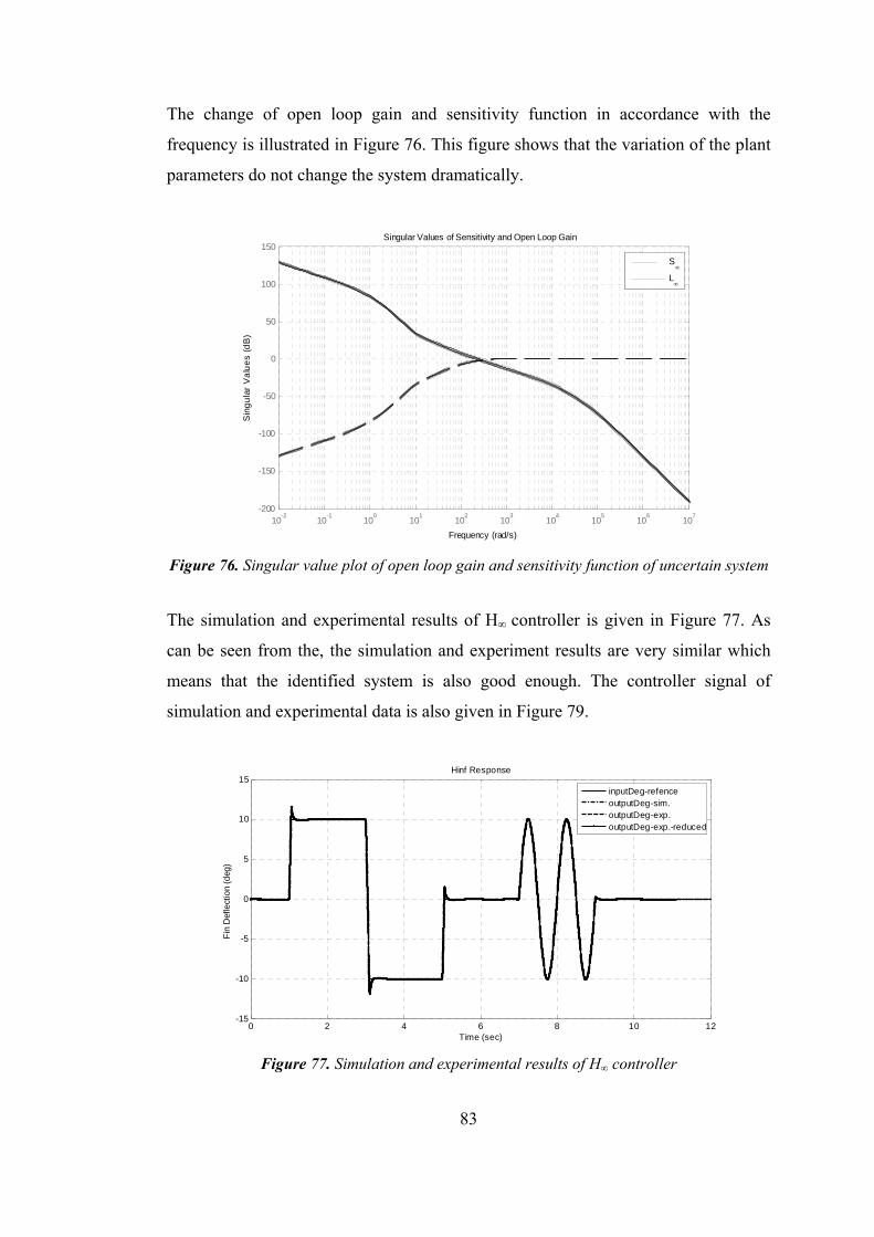
83
The change of open loop gain and sensitivity function in accordance with the
frequency is illustrated in Figure 76. This figure shows that the variation of the plant
parameters do not change the system dramatically.
Figure 76. Singular value plot of open loop gain and sensitivity function of uncertain system
The simulation and experimental results of H∞ controller is given in Figure 77. As
can be seen from the, the simulation and experiment results are very similar which
means that the identified system is also good enough. The controller signal of
simulation and experimental data is also given in Figure 79.
Figure 77. Simulation and experimental results of H∞ controller
10-2
10-1
100
101
102
103
104
105
106
107
-200
-150
-100
-50
0
50
100
150
Singular Values of Sensitivity and Open Loop Gain
Frequency (rad/s)
Sin
gu
lar
Va
lue
s (d
B)
S
L
0 2 4 6 8 10 12-15
-10
-5
0
5
10
15Hinf Response
Time (sec)
Fin
Def
lect
ion
(deg
)
inputDeg-refenceoutputDeg-sim.outputDeg-exp.outputDeg-exp.-reduced
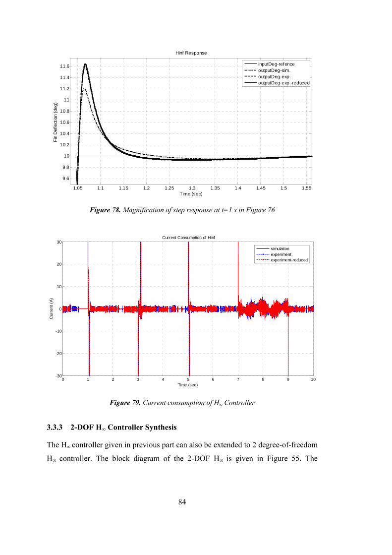
84
Figure 78. Magnification of step response at t=1 s in Figure 76
Figure 79. Current consumption of H∞ Controller
3.3.3 2-DOF H∞ Controller Synthesis
The H∞ controller given in previous part can also be extended to 2 degree-of-freedom
H∞ controller. The block diagram of the 2-DOF H∞ is given in Figure 55. The
1.05 1.1 1.15 1.2 1.25 1.3 1.35 1.4 1.45 1.5 1.55
9.6
9.8
10
10.2
10.4
10.6
10.8
11
11.2
11.4
11.6
Hinf Response
Time (sec)
Fin
Def
lect
ion
(deg
)
inputDeg-refenceoutputDeg-sim.outputDeg-exp.outputDeg-exp.-reduced
0 1 2 3 4 5 6 7 8 9 10-30
-20
-10
0
10
20
30Current Consumption of Hinf
Time (sec)
Cur
rent
(A
)
simulationexperimentexperiment-reduced
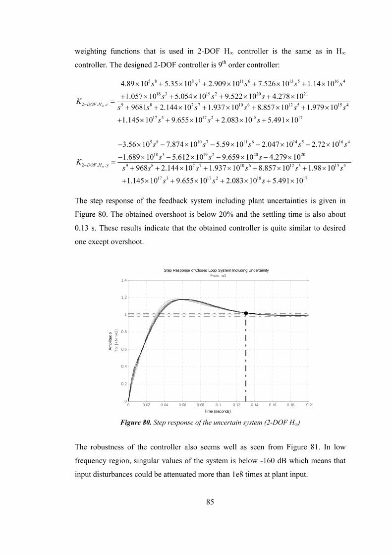
85
weighting functions that is used in 2-DOF H∞ controller is the same as in H∞
controller. The designed 2-DOF controller is 9th order controller:
5 8 8 7 11 6 13 5 16 4
18 3 19 2 20 21
2 . . 9 8 7 7 10 6 12 5 15 4
17 3
4.89 10 5.35 10 2.909 10 7.526 10 1.14 10
1.057 10 5.054 10 9.522 10 4.278 10
9681 2.144 10 1.937 10 8.857 10 1.979 10
1.145 10 9.655
DOF H r
s s s s s
s s sK
s s s s s s
s
17 2 18 17
5 8 10 7 11 6 14 5 16 4
18 3 19 2 20 20
2 . .y 9 8 7 7 10 6 12 5
10 2.083 10 5.491 10
3.56 10 7.874 10 5.59 10 2.047 10 2.72 10
1.689 10 5.612 10 9.659 10 4.279 10
968 2.144 10 1.937 10 8.857 10 1.DOF H
s s
s s s s s
s s sK
s s s s s
15 4
17 3 17 2 18 17
98 10
1.145 10 9.655 10 2.083 10 5.491 10
s
s s s
The step response of the feedback system including plant uncertainties is given in
Figure 80. The obtained overshoot is below 20% and the settling time is also about
0.13 s. These results indicate that the obtained controller is quite similar to desired
one except overshoot.
Figure 80. Step response of the uncertain system (2-DOF H∞)
The robustness of the controller also seems well as seen from Figure 81. In low
frequency region, singular values of the system is below -160 dB which means that
input disturbances could be attenuated more than 1e8 times at plant input.
0 0.02 0.04 0.06 0.08 0.1 0.12 0.14 0.16 0.18 0.20
0.2
0.4
0.6
0.8
1
1.2
1.4From: w1
To:
[+
Nin
v2]
Step Response of Closed Loop System Including Uncertainity
Time (seconds)
Am
plit
ude
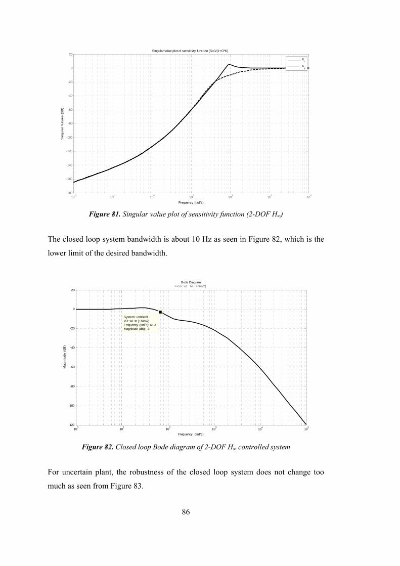
86
Figure 81. Singular value plot of sensitivity function (2-DOF H∞)
The closed loop system bandwidth is about 10 Hz as seen in Figure 82, which is the
lower limit of the desired bandwidth.
Figure 82. Closed loop Bode diagram of 2-DOF H∞ controlled system
For uncertain plant, the robustness of the closed loop system does not change too
much as seen from Figure 83.
10-2
10-1
100
101
102
103
104
-180
-160
-140
-120
-100
-80
-60
-40
-20
0
20
Singular value plot of sensitivity function (S=1/(1+G*K)
Frequency (rad/s)
Sin
gu
lar
Va
lue
s (d
B)
Kr
Ky
Bode Diagram
Frequency (rad/s)
100
101
102
103
104
105
-120
-100
-80
-60
-40
-20
0
20
System: untitled1I/O: w1 to [+Ninv2]Frequency (rad/s): 68.3Magnitude (dB): -3
From: w1 To: [+Ninv2]
Mag
nitu
de
(dB
)
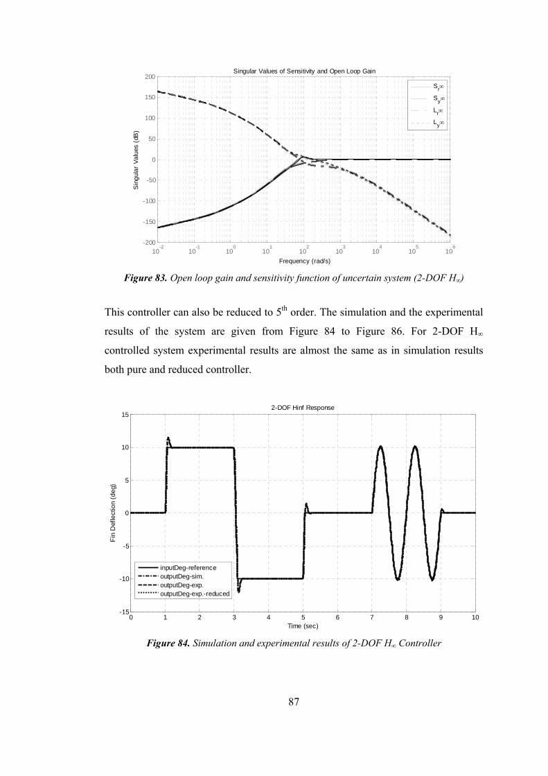
87
Figure 83. Open loop gain and sensitivity function of uncertain system (2-DOF H∞)
This controller can also be reduced to 5th order. The simulation and the experimental
results of the system are given from Figure 84 to Figure 86. For 2-DOF H∞
controlled system experimental results are almost the same as in simulation results
both pure and reduced controller.
Figure 84. Simulation and experimental results of 2-DOF H∞ Controller
10-2
10-1
100
101
102
103
104
105
106
-200
-150
-100
-50
0
50
100
150
200
Singular Values of Sensitivity and Open Loop Gain
Frequency (rad/s)
Sin
gu
lar
Va
lues
(dB
)
Sr
Sy
Lr
Ly
0 1 2 3 4 5 6 7 8 9 10-15
-10
-5
0
5
10
152-DOF Hinf Response
Time (sec)
Fin
Def
lect
ion
(d
eg)
inputDeg-referenceoutputDeg-sim.outputDeg-exp.outputDeg-exp.-reduced
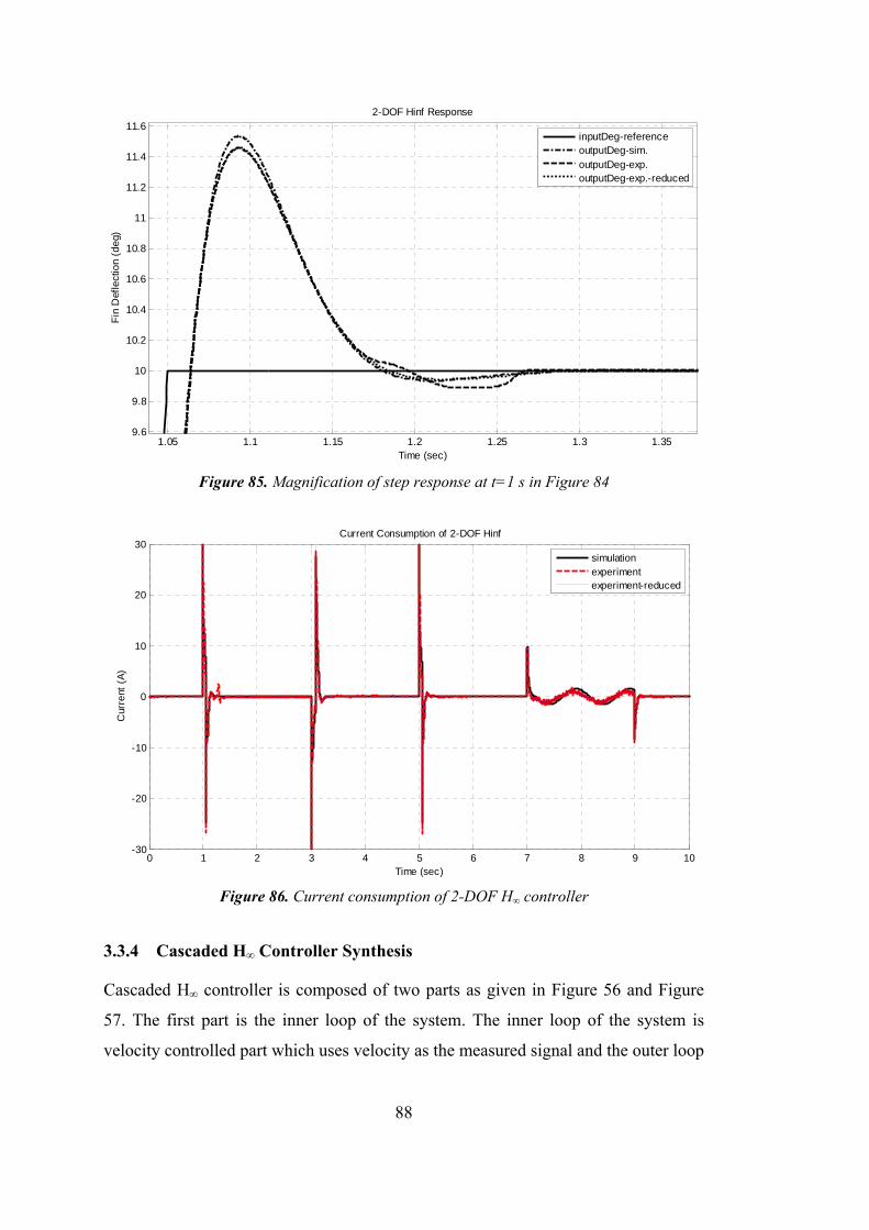
88
Figure 85. Magnification of step response at t=1 s in Figure 84
Figure 86. Current consumption of 2-DOF H∞ controller
3.3.4 Cascaded H∞ Controller Synthesis
Cascaded H∞ controller is composed of two parts as given in Figure 56 and Figure
57. The first part is the inner loop of the system. The inner loop of the system is
velocity controlled part which uses velocity as the measured signal and the outer loop
1.05 1.1 1.15 1.2 1.25 1.3 1.359.6
9.8
10
10.2
10.4
10.6
10.8
11
11.2
11.4
11.62-DOF Hinf Response
Time (sec)
Fin
Def
lect
ion
(de
g)
inputDeg-referenceoutputDeg-sim.outputDeg-exp.outputDeg-exp.-reduced
0 1 2 3 4 5 6 7 8 9 10-30
-20
-10
0
10
20
30Current Consumption of 2-DOF Hinf
Time (sec)
Cur
rent
(A
)
simulationexperimentexperiment-reduced
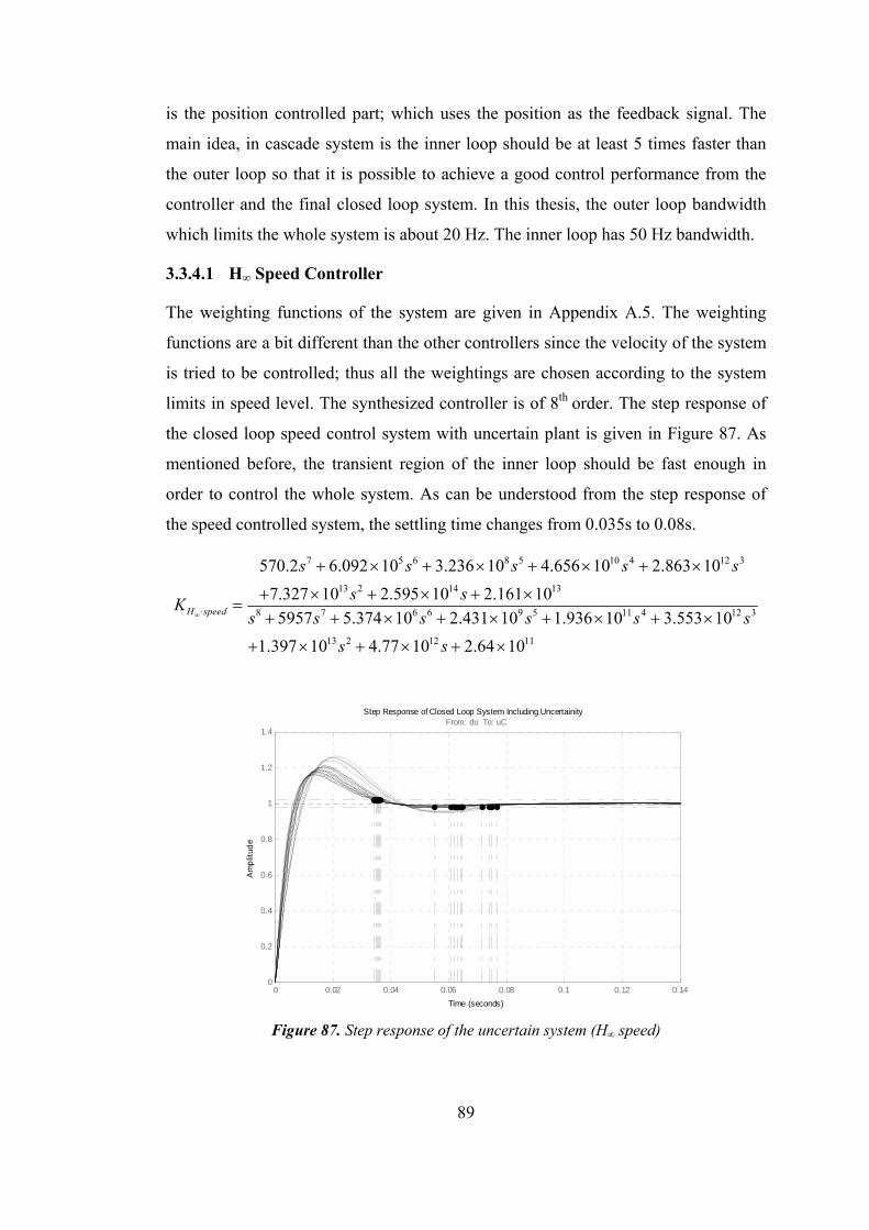
89
is the position controlled part; which uses the position as the feedback signal. The
main idea, in cascade system is the inner loop should be at least 5 times faster than
the outer loop so that it is possible to achieve a good control performance from the
controller and the final closed loop system. In this thesis, the outer loop bandwidth
which limits the whole system is about 20 Hz. The inner loop has 50 Hz bandwidth.
3.3.4.1 H∞ Speed Controller
The weighting functions of the system are given in Appendix A.5. The weighting
functions are a bit different than the other controllers since the velocity of the system
is tried to be controlled; thus all the weightings are chosen according to the system
limits in speed level. The synthesized controller is of 8th order. The step response of
the closed loop speed control system with uncertain plant is given in Figure 87. As
mentioned before, the transient region of the inner loop should be fast enough in
order to control the whole system. As can be understood from the step response of
the speed controlled system, the settling time changes from 0.035s to 0.08s.
7 5 6 8 5 10 4 12 3
13 2 14 13
8 7 6 6 9 5 11 4 12 3
13 2 12 11
570.2 6.092 10 3.236 10 4.656 10 2.863 10
7.327 10 2.595 10 2.161 10
5957 5.374 10 2.431 10 1.936 10 3.553 10
1.397 10 4.77 10 2.64 10
H speed
s s s s s
s sK
s s s s s s
s s
Figure 87. Step response of the uncertain system (H∞ speed)
Step Response of Closed Loop System Including Uncertainity
Time (seconds)
Am
plit
ude
0 0.02 0.04 0.06 0.08 0.1 0.12 0.140
0.2
0.4
0.6
0.8
1
1.2
1.4From: du To: uC
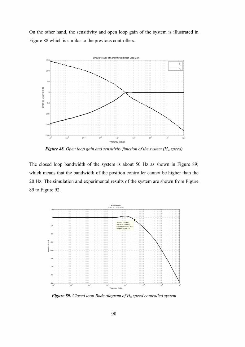
90
On the other hand, the sensitivity and open loop gain of the system is illustrated in
Figure 88 which is similar to the previous controllers.
Figure 88. Open loop gain and sensitivity function of the system (H∞ speed)
The closed loop bandwidth of the system is about 50 Hz as shown in Figure 89;
which means that the bandwidth of the position controller cannot be higher than the
20 Hz. The simulation and experimental results of the system are shown from Figure
89 to Figure 92.
Figure 89. Closed loop Bode diagram of H∞ speed controlled system
10-3
10-2
10-1
100
101
102
103
104
105
-200
-150
-100
-50
0
50
100
150
Singular Values of Sensitivity and Open Loop Gain
Frequency (rad/s)
Sin
gu
lar
Va
lue
s (d
B)
S
L
Bode Diagram
Frequency (rad/s)
10-2
10-1
100
101
102
103
104
105
-80
-70
-60
-50
-40
-30
-20
-10
0
10
System: untitled1I/O: w1 to [+Ninv2]Frequency (rad/s): 324Magnitude (dB): -3
From: w1 To: [+Ninv2]
Mag
nitu
de
(dB
)
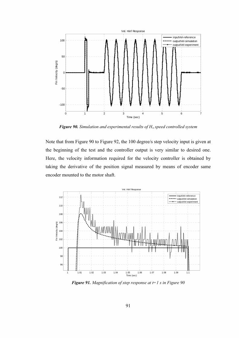
91
Figure 90. Simulation and experimental results of H∞ speed controlled system
Note that from Figure 90 to Figure 92, the 100 degree/s step velocity input is given at
the beginning of the test and the controller output is very similar to desired one.
Here, the velocity information required for the velocity controller is obtained by
taking the derivative of the position signal measured by means of encoder same
encoder mounted to the motor shaft.
Figure 91. Magnification of step response at t=1 s in Figure 90
0 1 2 3 4 5 6 7
-100
-50
0
50
100
Vel. Hinf Response
Time (sec)
Fin
Vel
oci
ty (
deg
/s)
inputVel-referenceoutputVel-simulationoutputVel-experiment
1 1.01 1.02 1.03 1.04 1.05 1.06 1.07 1.08 1.09 1.1
96
98
100
102
104
106
108
110
112
Vel. Hinf Response
Time (sec)
Fin
Vel
ocity
(de
g/s
)
inputVel-referenceoutputVel-simulationoutputVel-experiment
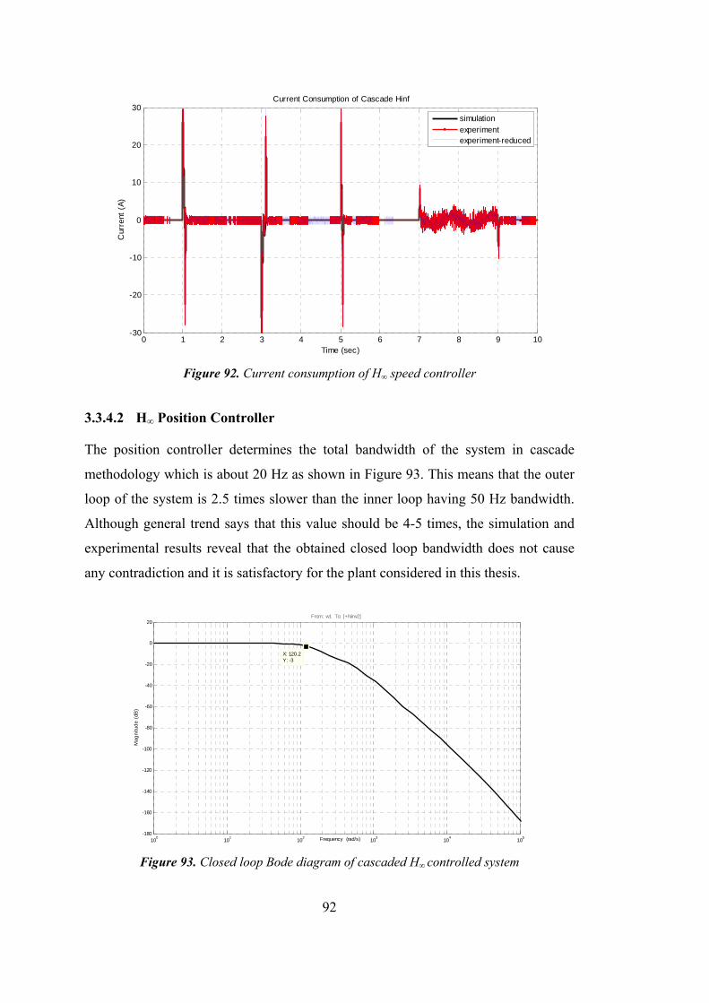
92
Figure 92. Current consumption of H∞ speed controller
3.3.4.2 H∞ Position Controller
The position controller determines the total bandwidth of the system in cascade
methodology which is about 20 Hz as shown in Figure 93. This means that the outer
loop of the system is 2.5 times slower than the inner loop having 50 Hz bandwidth.
Although general trend says that this value should be 4-5 times, the simulation and
experimental results reveal that the obtained closed loop bandwidth does not cause
any contradiction and it is satisfactory for the plant considered in this thesis.
Figure 93. Closed loop Bode diagram of cascaded H∞ controlled system
0 1 2 3 4 5 6 7 8 9 10-30
-20
-10
0
10
20
30Current Consumption of Cascade Hinf
Time (sec)
Cur
rent
(A
)
simulationexperimentexperiment-reduced
Frequency (rad/s)100
101
102
103
104
105
-180
-160
-140
-120
-100
-80
-60
-40
-20
0
20
X: 120.2Y: -3
From: w1 To: [+Ninv2]
Mag
nitu
de
(dB
)
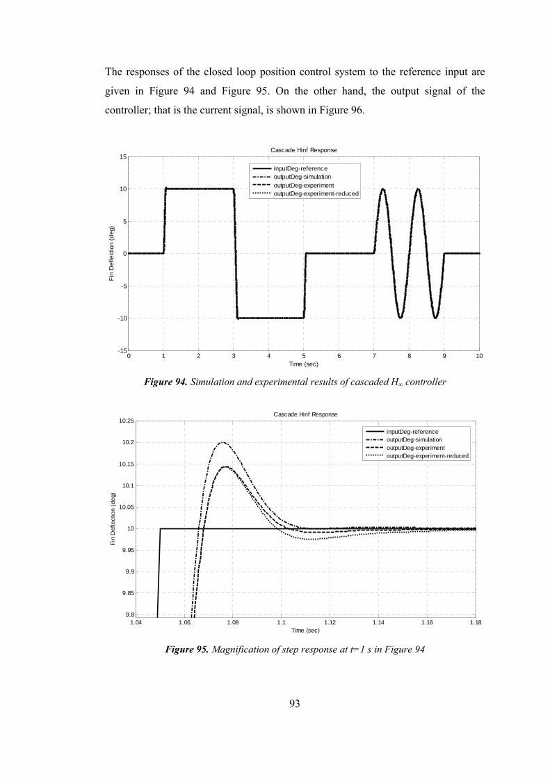
93
The responses of the closed loop position control system to the reference input are
given in Figure 94 and Figure 95. On the other hand, the output signal of the
controller; that is the current signal, is shown in Figure 96.
Figure 94. Simulation and experimental results of cascaded H∞ controller
Figure 95. Magnification of step response at t=1 s in Figure 94
0 1 2 3 4 5 6 7 8 9 10-15
-10
-5
0
5
10
15Cascade Hinf Response
Time (sec)
Fin
Def
lect
ion
(d
eg)
inputDeg-referenceoutputDeg-simulationoutputDeg-experimentoutputDeg-experiment-reduced
1.04 1.06 1.08 1.1 1.12 1.14 1.16 1.189.8
9.85
9.9
9.95
10
10.05
10.1
10.15
10.2
10.25Cascade Hinf Response
Time (sec)
Fin
Def
lect
ion
(d
eg)
inputDeg-referenceoutputDeg-simulationoutputDeg-experimentoutputDeg-experiment-reduced
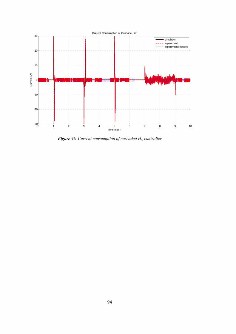
94
Figure 96. Current consumption of cascaded H∞ controller
0 1 2 3 4 5 6 7 8 9 10-30
-20
-10
0
10
20
30Current Consumption of Cascade Hinf
Time (sec)
Cur
rent
(A
)
simulationexperimentexperiment-reduced
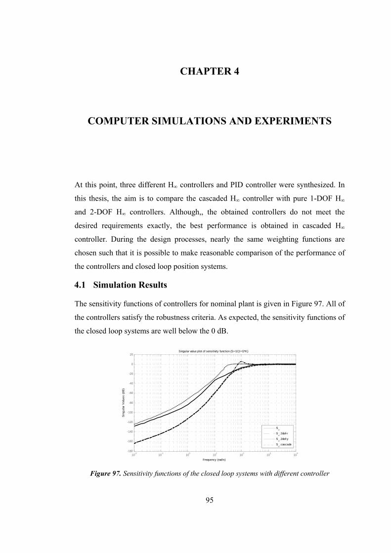
95
CHAPTER 4
COMPUTER SIMULATIONS AND EXPERIMENTS
At this point, three different H∞ controllers and PID controller were synthesized. In
this thesis, the aim is to compare the cascaded H∞ controller with pure 1-DOF H∞
and 2-DOF H∞ controllers. Although,, the obtained controllers do not meet the
desired requirements exactly, the best performance is obtained in cascaded H∞
controller. During the design processes, nearly the same weighting functions are
chosen such that it is possible to make reasonable comparison of the performance of
the controllers and closed loop position systems.
4.1 Simulation Results
The sensitivity functions of controllers for nominal plant is given in Figure 97. All of
the controllers satisfy the robustness criteria. As expected, the sensitivity functions of
the closed loop systems are well below the 0 dB.
Figure 97. Sensitivity functions of the closed loop systems with different controller
10-2
10-1
100
101
102
103
104
-180
-160
-140
-120
-100
-80
-60
-40
-20
0
20
Singular value plot of sensitivity function (S=1/(1+G*K)
Frequency (rad/s)
Sin
gu
lar
Va
lue
s (d
B)
S
S.2dof-r
S.2dof-y
S.cascade
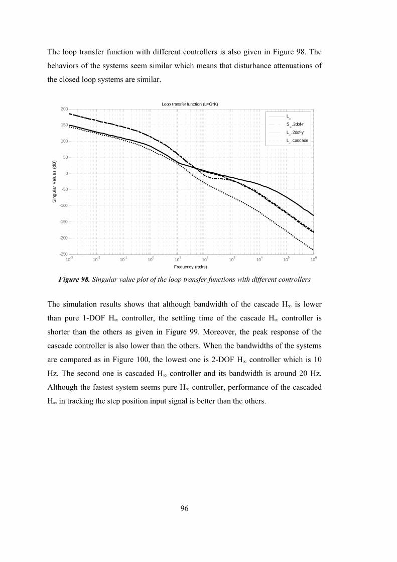
96
The loop transfer function with different controllers is also given in Figure 98. The
behaviors of the systems seem similar which means that disturbance attenuations of
the closed loop systems are similar.
Figure 98. Singular value plot of the loop transfer functions with different controllers
The simulation results shows that although bandwidth of the cascade H∞ is lower
than pure 1-DOF H∞ controller, the settling time of the cascade H∞ controller is
shorter than the others as given in Figure 99. Moreover, the peak response of the
cascade controller is also lower than the others. When the bandwidths of the systems
are compared as in Figure 100, the lowest one is 2-DOF H∞ controller which is 10
Hz. The second one is cascaded H∞ controller and its bandwidth is around 20 Hz.
Although the fastest system seems pure H∞ controller, performance of the cascaded
H∞ in tracking the step position input signal is better than the others.
10-3
10-2
10-1
100
101
102
103
104
105
106
-250
-200
-150
-100
-50
0
50
100
150
200
Loop transfer function (L=G*K)
Frequency (rad/s)
Sin
gu
lar
Va
lue
s (d
B)
L
S.2dof-r
L.2dof-y
L.cascade
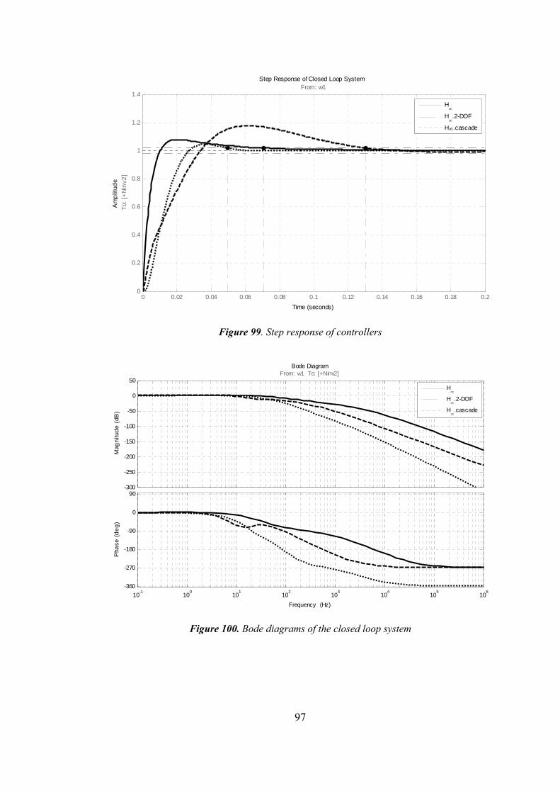
97
Figure 99. Step response of controllers
Figure 100. Bode diagrams of the closed loop system
0 0.02 0.04 0.06 0.08 0.1 0.12 0.14 0.16 0.18 0.20
0.2
0.4
0.6
0.8
1
1.2
1.4From: w1
To:
[+
Nin
v2]
Step Response of Closed Loop System
Time (seconds)
Am
plit
ude
H
H.2-DOF
H.cascade
-300
-250
-200
-150
-100
-50
0
50From: w1 To: [+Ninv2]
Mag
nitu
de
(dB
)
10-1
100
101
102
103
104
105
106
-360
-270
-180
-90
0
90
Pha
se (
de
g)
Bode Diagram
Frequency (Hz)
H
H.2-DOF
H.cascade
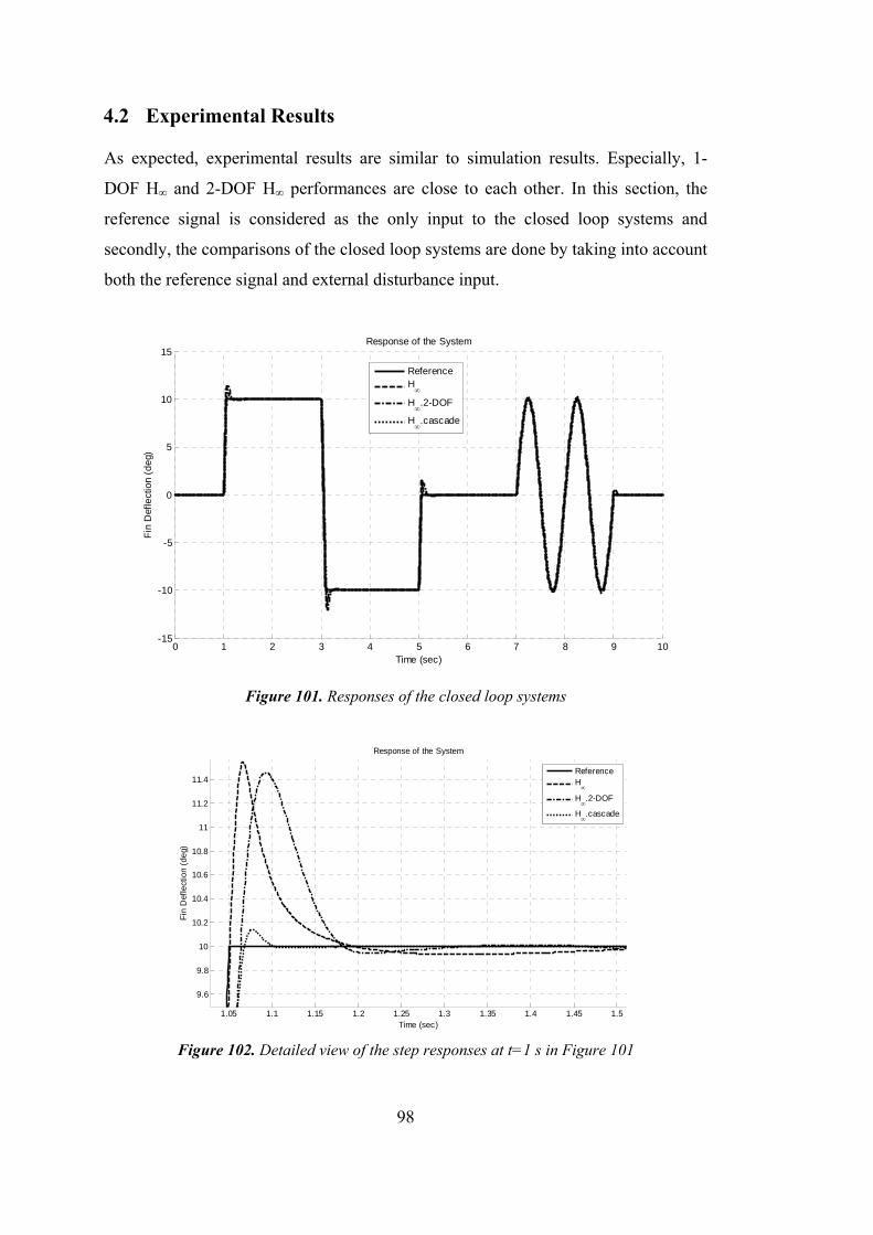
98
4.2 Experimental Results
As expected, experimental results are similar to simulation results. Especially, 1-
DOF H∞ and 2-DOF H∞ performances are close to each other. In this section, the
reference signal is considered as the only input to the closed loop systems and
secondly, the comparisons of the closed loop systems are done by taking into account
both the reference signal and external disturbance input.
Figure 101. Responses of the closed loop systems
Figure 102. Detailed view of the step responses at t=1 s in Figure 101
0 1 2 3 4 5 6 7 8 9 10-15
-10
-5
0
5
10
15
Time (sec)
Fin
Def
lect
ion
(d
eg)
Response of the System
ReferenceH
H
.2-DOF
H
.cascade
1.05 1.1 1.15 1.2 1.25 1.3 1.35 1.4 1.45 1.5
9.6
9.8
10
10.2
10.4
10.6
10.8
11
11.2
11.4
Time (sec)
Fin
Def
lect
ion
(d
eg)
Response of the System
ReferenceH
H
.2-DOF
H
.cascade
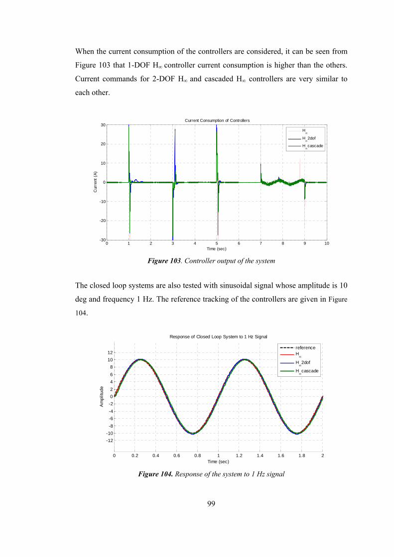
99
When the current consumption of the controllers are considered, it can be seen from
Figure 103 that 1-DOF H∞ controller current consumption is higher than the others.
Current commands for 2-DOF H∞ and cascaded H∞ controllers are very similar to
each other.
Figure 103. Controller output of the system
The closed loop systems are also tested with sinusoidal signal whose amplitude is 10
deg and frequency 1 Hz. The reference tracking of the controllers are given in Figure
104.
Figure 104. Response of the system to 1 Hz signal
0 1 2 3 4 5 6 7 8 9 10-30
-20
-10
0
10
20
30
Time (sec)
Cur
rent
(A
)
Current Consumption of Controllers
H
H
2dof
H
cascade
0 0.2 0.4 0.6 0.8 1 1.2 1.4 1.6 1.8 2
-12
-10
-8
-6
-4
-2
0
2
4
6
8
10
12
Time (sec)
Am
plit
ude
Response of Closed Loop System to 1 Hz Signal
referenceH
H2dof
Hcascade
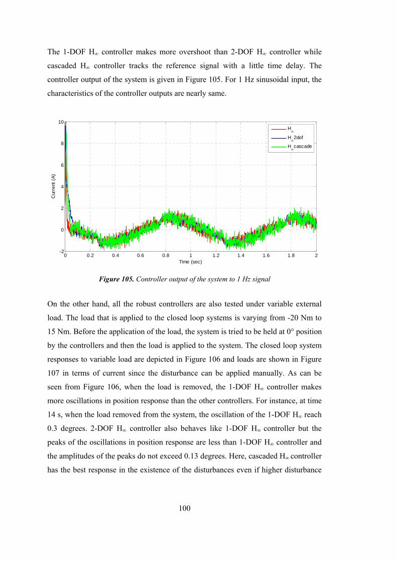
100
The 1-DOF H∞ controller makes more overshoot than 2-DOF H∞ controller while
cascaded H∞ controller tracks the reference signal with a little time delay. The
controller output of the system is given in Figure 105. For 1 Hz sinusoidal input, the
characteristics of the controller outputs are nearly same.
Figure 105. Controller output of the system to 1 Hz signal
On the other hand, all the robust controllers are also tested under variable external
load. The load that is applied to the closed loop systems is varying from -20 Nm to
15 Nm. Before the application of the load, the system is tried to be held at 0° position
by the controllers and then the load is applied to the system. The closed loop system
responses to variable load are depicted in Figure 106 and loads are shown in Figure
107 in terms of current since the disturbance can be applied manually. As can be
seen from Figure 106, when the load is removed, the 1-DOF H∞ controller makes
more oscillations in position response than the other controllers. For instance, at time
14 s, when the load removed from the system, the oscillation of the 1-DOF H∞ reach
0.3 degrees. 2-DOF H∞ controller also behaves like 1-DOF H∞ controller but the
peaks of the oscillations in position response are less than 1-DOF H∞ controller and
the amplitudes of the peaks do not exceed 0.13 degrees. Here, cascaded H∞ controller
has the best response in the existence of the disturbances even if higher disturbance
0 0.2 0.4 0.6 0.8 1 1.2 1.4 1.6 1.8 2-2
0
2
4
6
8
10
Time (sec)
Cur
rent
(A
)
H
H
2dof
H
cascade
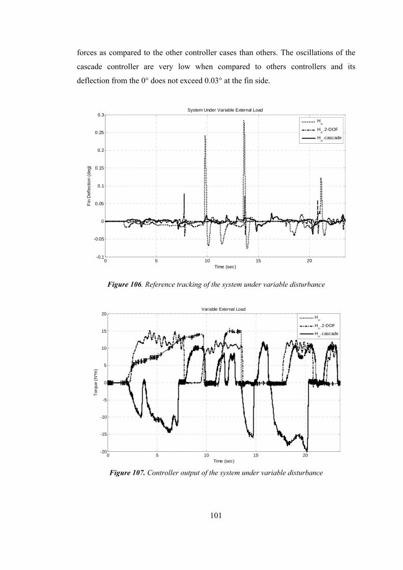
101
forces as compared to the other controller cases than others. The oscillations of the
cascade controller are very low when compared to others controllers and its
deflection from the 0° does not exceed 0.03° at the fin side.
Figure 106. Reference tracking of the system under variable disturbance
Figure 107. Controller output of the system under variable disturbance
0 5 10 15 20-0.1
-0.05
0
0.05
0.1
0.15
0.2
0.25
0.3
Time (sec)
Fin
Def
lect
ion
(d
eg)
System Under Variable External Load
H
H
.2-DOF
H
.cascade
0 5 10 15 20-20
-15
-10
-5
0
5
10
15
20
Time (sec)
Tor
qu
e (N
*m)
Variable External Load
H
H
.2-DOF
H
.cascade
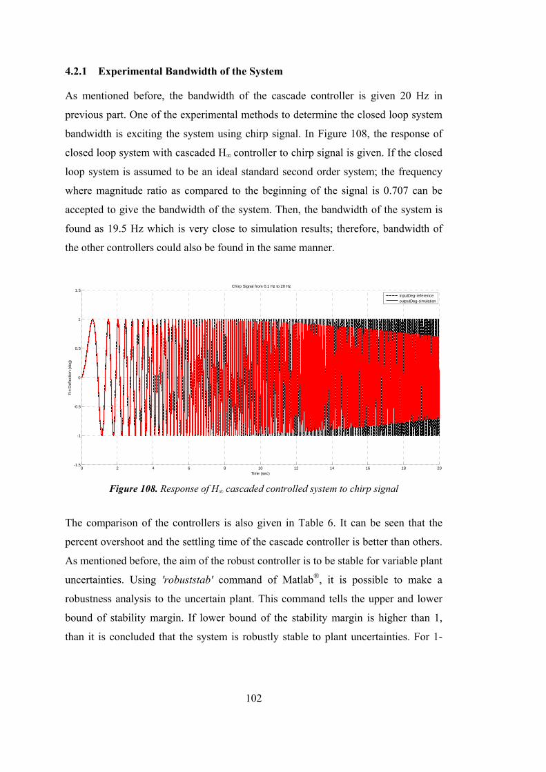
102
4.2.1 Experimental Bandwidth of the System
As mentioned before, the bandwidth of the cascade controller is given 20 Hz in
previous part. One of the experimental methods to determine the closed loop system
bandwidth is exciting the system using chirp signal. In Figure 108, the response of
closed loop system with cascaded H∞ controller to chirp signal is given. If the closed
loop system is assumed to be an ideal standard second order system; the frequency
where magnitude ratio as compared to the beginning of the signal is 0.707 can be
accepted to give the bandwidth of the system. Then, the bandwidth of the system is
found as 19.5 Hz which is very close to simulation results; therefore, bandwidth of
the other controllers could also be found in the same manner.
Figure 108. Response of H∞ cascaded controlled system to chirp signal
The comparison of the controllers is also given in Table 6. It can be seen that the
percent overshoot and the settling time of the cascade controller is better than others.
As mentioned before, the aim of the robust controller is to be stable for variable plant
uncertainties. Using 'robuststab' command of Matlab®, it is possible to make a
robustness analysis to the uncertain plant. This command tells the upper and lower
bound of stability margin. If lower bound of the stability margin is higher than 1,
than it is concluded that the system is robustly stable to plant uncertainties. For 1-
0 2 4 6 8 10 12 14 16 18 20-1.5
-1
-0.5
0
0.5
1
1.5
Time (sec)
Fin
Def
lect
ion
(de
g)
Chirp Signal from 0.1 Hz to 20 Hz
inputDeg-referenceoutputDeg-simulation
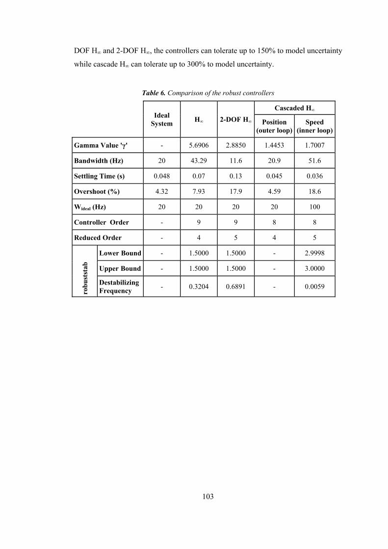
103
DOF H∞ and 2-DOF H∞, the controllers can tolerate up to 150% to model uncertainty
while cascade H∞ can tolerate up to 300% to model uncertainty.
Table 6. Comparison of the robust controllers
Ideal
System H∞ 2-DOF H∞
Cascaded H∞
Position (outer loop)
Speed (inner loop)
Gamma Value 'γ' - 5.6906 2.8850 1.4453 1.7007
Bandwidth (Hz) 20 43.29 11.6 20.9 51.6
Settling Time (s) 0.048 0.07 0.13 0.045 0.036
Overshoot (%) 4.32 7.93 17.9 4.59 18.6
Wideal (Hz) 20 20 20 20 100
Controller Order - 9 9 8 8
Reduced Order - 4 5 4 5
rob
ust
stab
Lower Bound - 1.5000 1.5000 - 2.9998
Upper Bound - 1.5000 1.5000 - 3.0000
Destabilizing Frequency
- 0.3204 0.6891 - 0.0059

104
105
CHAPTER 5
DISCUSSION AND CONCLUSION
5.1 Summary and Comments on the Results
In this study, modeling, identification, simulations, and experiments of the control
system for a fin actuation system is studied. In this respect, firstly PID controllers are
designed and their performance are compared. Then, 1-DOF, 2-DOF, and cascaded
H∞ controllers are synthesized. All the controllers are simulated in computer
environment and then these controllers are applied to physical system.
In order to make experiments, initially, the mathematical model of the system is
obtained. In this section, the electrical part of the system is neglected because of the
very high band width frequency of the driver card. This simplified model is used
both on identification and simulation parts. The obtained mathematical model is tired
to be verified using a standard system identification procedure. In this respect, PRBS
and BLWN signals are applied to system as the input. The obtained input/output data
set is firstly converted to frequency domain and then all the identification procedure
is carried out in frequency domain. The identified model appeared to be a second
order system with a free integrator. This model is obtained in two ways. In first way,
all the parameters are assumed unknown and found in certain intervals. In second
way, the motor torque constant and equivalent inertia of the system are computed
and using these values equivalent viscous friction of the system is estimated. In
controller synthesis, the first way is chosen.
As mentioned before, three different PID and H∞ controllers are synthesized. In first
PID, Butterworth polynomials are used in order to place the poles of the closed loop
106
control system as per the desired bandwidth and nondimensional damping quantities.
This way, it becomes possible to find the gains of the controller. The second one is
designed using 'pidtool' command of Matlab®. The final PID controller is obtained
using experimental approach. In this PID, Ziegler-Nichols tuning method is utilized
to determine the controller gains. The simulation and experimental results show that
the current consumption of PID controllers is higher than their robust counterparts.
The performance of the PID controllers is a bit lower than expected. Thus, in Chapter
4, the PID controllers are not compared with the robust controllers. After that, H∞
controllers are designed, simulated and tested. The weighting functions of H∞
controllers are decided according to physical performance requirements and physical
limits of the system. For 1-DOF and 2-DOF controllers same weighting functions are
used but for the cascaded controller, weighting functions are redefined according to
speed requirements of system for inner loop and position requirements of the speed
for the outer loop. The order of H∞ controllers is generally higher than the classical
controllers so that one may think that, the cascade controller is unnecessary since its
degree is much higher than the other H∞ controllers and the speed feedback can lead
to some problems during operation. The important point is that the aim of this thesis
is not mainly to find the best controller but to find a new representation for naturally
nonlinear systems. Furthermore, the uncertainties are defined on the whole plant
instead of defining on each parameter which causes problems during the synthesis of
the controllers in this thesis. The gamma values of the robust controllers are a bit
higher than unity which may cause robustness problem on real applications but this
situation can be guaranteed using a robust stability analysis. On the other hand, inner
loop of the cascade controller; that is speed loop, could also be reduced to a second
order system after its closed loop speed control is achieved so that the order of the
position controller can be reduced significantly.
To sum up, the cascaded controller that handled in this thesis can be an alternative
controller for the electromechanical actuator systems.
5.2 Future Works
In this study, jet vane parts are not physically constructed. Indeed, the jet vane part is
taken as a disturbing torque on the system. As a first future work, the jet vane part

107
can be integrated to the real system and the controller performance can also be tested.
In addition to this, as an alternative to the performance and ideal closed loop
weightings, an additional performance weighting representing the error between
reference input and measured output could also be assigned for robust controller
synthesis. Thus, an unnecessary increase in controller order could be reduced and
more optimized and easy to implement controllers could be designed. As an another
future work, other ways of representing uncertainty in parametric level could also be
improved for the future works. Eventually, load test can also be made in controlled
speed and load conditions. To summarize, the future works to be done can be written
as:
integration of jet vanes to the physical system
decision of alternative weighting functions between error and reference input
reduction of controller orders
optimization of controllers to decrease current consumption
changing of uncertainty definition
load test under controllable speed and torque

108
109
REFERENCES
[1] Fleeman, E. L., "Air-to-Air Missile Design and System Engineering Short
Course," Ankara, 2013.
[2] Siouris, G. M., Missile Guidance and Control Systems, New York: Springer,
2004.
[3] Sutton, G. P., Biblarz, O., Rocket Propulsion Elements, John Wliey & Sons,
Inc., 2001.
[4] "Air-Launched Weapons," IHS Jane's 360, [Online]. Available:
http://www.janes.com/. [Accessed 20 May 2013].
[5] Control Actuation Workshop/System Engineering, Martin Marietta Training
Notes, 1993.
[6] Chin, S. S., Missile Configuration Design, McGraw-Hill Book Company, Inc.,
1961.
[7] Fleeman, E. L., Tactical Missile Design, Virginia: American Institute of
Aeronautics and Astronautics, Inc., 2001.
[8] Mark, H., Encyclopedia of Space Science and Technology, vol. I, New Jersey:
John Wiley & Sons, Inc., 2003.
[9] "Solid Rocket Thrust Vector Control," NASA, 1974.
[10] Yangel, M., Thrust Vector and Aerodynamic Control of Missiles, Msc Thesis:
METU, Ankara, Turkey, 1995.
[11] Llyod, R., "A Review of Thrust Vector Control Systems for Tactical Missiles,"
in AAIA/SAE Joint Propulsion Conferans, Las Vegas, 1978.
110
[12] TVC Jet Vane Thermal Modelling Using Parametric System Identification,
NPS69-88-001: Naval Post Graduate School, 1988.
[13] Schaefermeyer, M. R., Aerodynamic Thrust Vectoring for Attitude Control of a
Vertically Thrusting Jet Engines, Utah, 2011.
[14] Balu, R., Marathe, A. G., Paul, P. J., Mukundas, H. S., "Analysis of
Performance of a Hot Gas Injection Thrust Vector Control System," J.
Propulsion, vol. 7, no. 4, pp. 580-585, 1991.
[15] "A4/V2 Makeup," Brothers Design, 1999. [Online]. Available:
http://www.v2rocket.com. [Accessed 10 June 2014].
[16] Design and Analysis of Solid Rocket Motor Nozzle, AGARD-LS-150, 1988.
[17] Yu, M. S., Cho, H. H., Hwang, K. Y., Bae, J. C., "A Study on a Surface
Ablation of the Jet Vane System in a Rocket Nozzle, AIAA-2004-2276," in
AIAA Thermophysics Conference, Portland, Oregon, 2004.
[18] El-Sharkawy, A. I., "Experimental Studies on Thrust Vector in Solid Propellant
Rockets," in AIAA/SAE Propulsion Conference, Orlando / Florida, 1977.
[19] Sung, H., Hwang, Y., "Thrust-Vector Characteristics of Jet Vanes Arranged in
X-Formation Within a Shroud," Journal of Propulsion and Power, vol. 20, no.
3, pp. 501-508, 2004.
[20] Facciano, A. B., Seybold, K. G., Westberry-Kutz, T. L., Widmer, D. O.,
"Evolved SeaSparrow Missile Jet Vane Control System Prototype Hardware
Development," Journal of Spacecraft and Rockets, vol. 39, no. 4, pp. 522-531,
2002.
[21] Kalnins, I., Gorlov, V., Gerhard, I., "The COSMOS Launch Services and
Launch System Modernization Program, AIAA-2001-4699," in AIAA Space
Conferance and Exposition, Albuquerque, 2001.
111
[22] Rainville, P., deChamplain, A., Kretschmer, D., Farinaccio, R., Stowe, R.,
"Unsteady CFD Calculation for Validation of a Multi-Vane Thrust Vector
Control System," in AIAA/ASME/SAE/ASEE Joint Propulsion Conference and
Exhibit, Florida, 2004.
[23] T. W. Bastian, "Jet Tab Control Mechanism for Thrust Vector Control". USA
Patent 4,274,610, 23 June 1981.
[24] Edwards, S.S., Parker, G.H., "An Investigation of the Jetevator as a Means of
Thrust Vector Control," Lockheed Missiles & Space Company Inc., California,
1958.
[25] Dumoulin, J., "Reaction Control System," 31 August 2000. [Online]. Available:
http://science.ksc.nasa.gov. [Accessed 2014 10 16].
[26] Innocenti, M., Thukral, A., "Simultaneous Reaction Jet and Aerodynamic
Control of Missile Systems," in Aerospace Design Conference, Irvine, CA,
1993.
[27] Machell A., Foulsham, P. G., "Reaction Control System". England Patent
4,955,558, 11 September 1990.
[28] Ellison, J. R., "Jet Tab Steerable Missile". USA Patent 3,986,683, 19 October
1976.
[29] Jacobson, M. D., "Droppable Jet Vane TVC". USA Patent 5,082,202, 21
January 1992.
[30] Kim, W. H., Bae, J. C., Lim, S. T., Park, S. H. "Jet Vane Thrust Vector Control
System". USA Patent US 7,313,910 B2, 1 January 2008.
[31] Hatalsky, W., Facciano, A., Haight, S. D., Jordan, A., "Jet Vane Control
System and Method". USA Patent 5,806,791, 15 September 1998.
[32] Doyle J., Francis B., Tannenbaum A., Feedback Control Theory, California,
112
Macmillan Publishing Co., 1990.
[33] Xue, D., Chen, Y., Atherton, D. P., Linear Feedback Control - Analysis and
Desing with Matlab, Philadelphia: SIAM, 2007.
[34] Zames, G., "Feedback and Optimal Sensitivity: Model Reference
Transformations, Multiplicative Seminorms, and Approximate Inverses," IEEE
Transactions on Automatic Control, vol. 26, no. 2, pp. 301-320, 1981.
[35] Doyle J., Glover K., Khargonekar P.P., Francis B.A., "State Space Solutions to
Standard H2 and H∞ Control Problems," IEEE Trans. on Automatic Control,
vol. 34, no. 8, pp. 831-847, 1989.
[36] Rollins, L., "Robust Control Theory," [Online]. Available:
http://users.ece.cmu.edu/. [Accessed 6 July 2014].
[37] Toscano, R., Structured Controllers for Uncertain Systems - A Stochastic
Optimizaion Approach, London: Springer-Verlag, 2013.
[38] Bibel, J. E., Malyevac, D. S., "Guidelines for the Selection of Weighting
Functions for H-Infinity Control NSWCDD/MP-92/43," Naval Surface Warfare
Center, Dahlgren, Virginia, 1992.
[39] Skogestad, S., Postlethwaite, I., "Multivariable Feedback Control - Analysis and
Design," John Wiley & Sons, 1996.
[40] Gu, D., Petkov, P. H., Konstantinov, M. M., Robust Control Design with
Matlab, London: Springer, 2013.
[41] Zhou, K., Doyle, J. C., Glover, K., Robust and Optimal Control, New Jersey:
Prentice Hall, 1996.
[42] Hartley, G. A., "H∞ Controller Design for an SISO Electromechanical
Actuator," in AIAA Guidance, Navigation and Control Conference, HiltonHilton
Head Island, SC, U.S.A., 1992.
113
[43] Hartley, G. A., "Comparison of Classical and H-infinity Controller Design for a
Single-axis Prototype Electromechanical Actuator," in AIAA Guidance,
Navigation and Control Conference, Monterey, CA, U.S.A., 1993.
[44] Malasse, O., Zasadzinski, M., Iung, C., Hayar, H., Darouach, M., "H∞ Design
Using Normalized Coprime Factors: An Application to an Electromechanical
Actuator," in IEEE Conference on Control Applications, Glasgow, UK, 1994.
[45] Adam, E. J., Guesrtrin, E. D., "Identification and Robust Control of an
Experimental Servo Motor," ISA Transactions, vol. 41, no. 2, pp. 225-234,
2002.
[46] Luo G., Fan, P., "Mixed H2/H∞ Control of Direct-Drive Electromechanical
Actuator," in International Conference on Electrical Machines and Systems,
Beijing, China, 2003.
[47] Ölçer, T. U., H2/H∞ Mixed Robust Controller Synthesis for a Fin Actuation
System, Msc Thesis: METU, Ankara, Turkey, 2013.
[48] Daş, E., Güdümlü Bir Mühimmat Kanatçık Tahrik Sistemi İçin İki Döngülü
Kontrol Sistemi Tasarımı, Msc Thesis: İTÜ, İstanbul, Turkey, 2014.
[49] Yoo, C. H., Lee, Y. C., Lee, S. Y., "A Robust Controller for an Electro-
Mechanical Fin Actuator," in Asian Control Conferance, Grand Hyatt-
Melbourne, Australia, 2004.
[50] Eker, İ., "Sliding Mode Control with PID Sliding Surface and Experimental
Application to an Electromechanical Plant," ISA Transactions, vol. 45, no. 1, pp.
109-118, 2006.
[51] Schinstock, D. E., Haskew, T. A., "Identifcation of Continuous-Time, Linear,
and Nonlinear Models of an Electromechanical Actuator," Journal of
Propulsion and Power, vol. 13, no. 5, pp. 683-690, 1997.
[52] Schinstock, D. E., Scott, D. A., Haskew, T. A., "Modeling and Estimation for
114
Electromechanical Thrust Vector Control of Rocket Engines," Journal of
Propulsion and Power, vol. 14, no. 4, pp. 440-446, 1998.
[53] Schinstock, D. E., Scott, D. A., Haskew, T. A., "Transient Force Reduction in
Electromechanical Actuators for Thrust Vector Control," Journal of Propulsion
and Power, vol. 17, no. 1, pp. 65-72, 2001.
[54] Ristanović, M., Lazić, D., Indin, I., "Experimental Validation of Improved
Performances of an Electromechanical Aerofin Control System with a PWM
Controlled DC Motor," FME Transactions, vol. 34, no. 1, pp. 15-20, 2006.
[55] Ristanović, M., Lazić, D., Indin, I., "Nonlinear PID Controller Modification of
Electromechanical Actuator System for Aerofin Control with PWM Controlled
DC Motor," Automatic Control and Robotics, vol. 7, no. 1, pp. 131-139, 2008.
[56] Lazić, D., Cojbasic, Z., Ristanović, M., "Fuzzy-Neuro-Genetic Aerofin
Control," Automatic Control and Robotics, vol. 10, no. 1, pp. 71-82, 2011.
[57] Ristanović, M., Lazić, D., Indin, I., "Intelligent Control of DC motor Driven
Electromechanical Fin Actuator," Control Engineering Practice, vol. 20, no. 6,
pp. 610-617, 2012.
[58] Jeong, D. S., Choi, K. J., Woo, H. W., Kim, J. G., "Controller Design of Missile
Actuator Using DSP," in International Conference on Control, Automation and
Systems, Seoul, Korea, 2007.
[59] Khan, M. A., Todić, I., Miloš, M., Stefanović, Z., Blagojević, Dj., "Control of
Electro-Mechanical Actuator for Aerospace Applications," Strojarstvo, vol. 52,
no. 3, pp. 303-313, 2010.
[60] Gao, Y., Gu, L., Pan, L., "Application of Variable Structure Control in Missile
Electromechanical Actuator System," in International Conference on Intelligent
Computation Technology and Automation, Changsha, Hunan, China, 2008.
[61] Yan L., Dongyang, S., "Research on Electro-Mechanical Actuator System
115
Based on Discrete-time Variable Structure Control," in WRI Global Congress on
Intelligent Systems, Wuhan, Hubei, China, 2010.
[62] Liu, X., Wu, Y., Deng, Y., Xiao, S., "A Global Sliding Mode Controller for
Missile Electromechanical Actuator Servo System," Journal of Aerospace
Engineering, vol. 228, no. 9, pp. 1-10, 2013.
[63] Dwivedula, R. V., Pagilla, P. R., "Effect of Compliance and Backlash on the
Output Speed of a Mechanical Transmission System," Journal of Dynamic
Systems, Measurement, and Control, vol. 134, no. 3, 2012.
[64] Nordin, M., Gutman, P. O., "Controlling Mechanical Systems with Backlash - A
Survey," Automatica, no. 38, pp. 1633-1649, 2002.
[65] Axsys Technologies, Brushless DC Motors Handbook, Axsys Technologies.
[66] ADVANCED Motion Controls, "Downloadable Resources," 1997. [Online].
Available: http://www.a-m-c.com. [Accessed 20 August 2014].
[67] Landau, I. D., Zito, G., Digital Control Systems - Design, Identification and
Implementation, Germany: Springer-Verlag London Limited, 2006.
[68] Söderström, T., Stoica, P., System Identification, Cambridge: Prentice Hall
Internatioal (UK) Ltd., 1989.
[69] "Selecting a Sampling Rate," National Instruments, June 2010. [Online].
Available: ni.com. [Accessed 12 June 2014].
[70] National Instruments, "Stimulus and Acquisition Considerations in the System
Identification Process," 17 June 2010. [Online]. Available: http://www.ni.com.
[Accessed 2014 August 26].
[71] Ljung, L., "System Identification Toolbox™ R2014b," Mathworks, 2014.
[72] Babuska, R., Fuzzy Modelling for Control, Boston: Kluwer academic
Publishers, 1988.
116
[73] Rogers, R., "Building a Benchtop PID Controller," 2013. [Online]. Available:
http://www.keithley.com/. [Accessed 29 July 2014].
[74] O'Dwyer, A., Handbook of PI and PID Controller Tuning Rules, London:
Imperial College Press, 2006.
[75] Özkan B., Dynamic Modeling, Guidance and Control of Missiles, Ph.D. Thesis:
METU, Ankara, Turkey, 2005.
[76] Fortuna L., Frasca M., Optimal and Robust Control Advanced Topics with
MATLAB, Florida, CRC Press, 2012.
[77] Beaven, R. W., Wright, M. T., Seaward, D. R., "Weighting Function Selection
in the H-infinity Design Process," Control Engineering Practice, vol. 4, no. 5,
pp. 625-633, 1996.
[78] Hu, J., Bohn, C., Wu, H. R., "Systematic H∞ Weighting Function Selection and
Its Application to the Real-time Control of a Vertical Take-of Aircraft," Control
Engineering Practice, vol. 8, pp. 241-252, 200.
[79] Grimble, M. J., Biss, D., "Selection of Optimal Control Weighting Functions to
Achieve Good H-infinity Designs," in International Conference on Control,
Oxford, 1988.
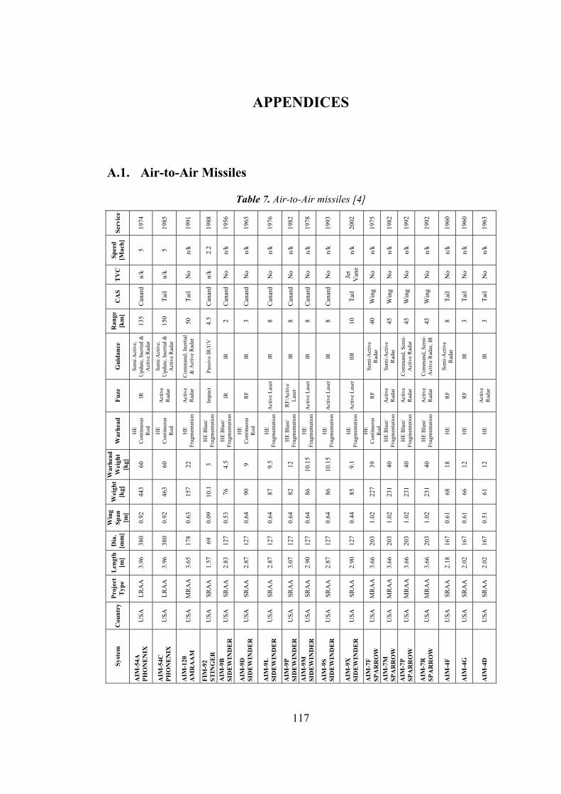
117
APPENDICES
A.1. Air-to-Air Missiles
Table 7. Air-to-Air missiles [4]
Ser
vice
1974
1985
1991
1988
1956
1965
1976
1982
1978
1993
2002
1975
1982
1992
1992
1960
1960
1963
Sp
eed
[Mac
h]
5 5 n/k
2.2
n/k
n/k
n/k
n/k
n/k
n/k
n/k
n/k
n/k
n/k
n/k
n/k
n/k
n/k
TV
C
n/k
n/k
No
n/k
No
No
No
No
No
No
Jet
Van
e
No
No
No
No
No
No
No
CA
S
Can
ard
Tai
l
Tai
l
Can
ard
Can
ard
Can
ard
Can
ard
Can
ard
Can
ard
Can
ard
Tai
l
Win
g
Win
g
Win
g
Win
g
Tai
l
Tai
l
Tai
l
Ran
ge
[km
]
135
150
50
4.5 2 3 8 8 8 8 10
40
45
45
45
8 3 3
Gu
idan
ce
Sem
i Act
ive,
U
pdat
e, I
nert
ial &
A
ctiv
e R
adar
Sem
i Act
ive,
U
pdat
e, I
nert
ial &
A
ctiv
e R
adar
Com
man
d, I
nert
ial
& A
ctiv
e R
adar
Pas
sive
IR
/UV
IR
IR
IR
IR
IR
IR
IIR
Sem
i-A
ctiv
e R
adar
Sem
i-A
ctiv
e R
adar
Com
man
d, S
emi-
Act
ive
Rad
ar
Com
man
d, S
emi-
Act
ive
Rad
ar, I
R
Sem
i-A
ctiv
e R
adar
IR
IR
Fu
ze
IR
Act
ive
Rad
ar
Act
ive
Rad
ar
Impa
ct
IR
RF
Act
ive
Las
er
RF
/Act
ive
Las
er
Act
ive
Las
er
Act
ive
Las
er
Act
ive
Las
er
RF
Act
ive
Rad
ar
Act
ive
Rad
ar
Act
ive
Rad
ar
RF
RF
Act
ive
Rad
ar
War
head
HE
C
onti
nuou
s R
od
HE
C
onti
nuou
s R
od
HE
F
ragm
enta
tion
HE
Bla
st/
Fra
gmen
tati
on
HE
Bla
st/
Fra
gmen
tati
on
HE
C
onti
nuou
s R
od
HE
F
ragm
enta
tion
HE
Bla
st/
Fra
gmen
tati
on
HE
F
ragm
enta
tion
HE
F
ragm
enta
tion
HE
F
ragm
enta
tion
HE
C
onti
nuou
s R
odH
E B
last
/ F
ragm
enta
tion
HE
Bla
st/
Fra
gmen
tati
on
HE
Bla
st/
Fra
gmen
tati
on
HE
HE
HE
War
head
W
eigh
t [k
g]
60
60
22
3 4.5 9 9.5
12
10.1
5
10.1
5
9.1
39
40
40
40
18
12
12
Wei
ght
[kg]
443
463
157
10.1
76
90
87
82
86
86
85
227
231
231
231
68
66
61
Win
g S
pan
[m
]
0.92
0.92
0.63
0.09
0.53
0.64
0.64
0.64
0.64
0.64
0.44
1.02
1.02
1.02
1.02
0.61
0.61
0.51
Dia
. [m
m]
380
380
178
69
127
127
127
127
127
127
127
203
203
203
203
167
167
167
Len
gth
[m]
3.96
3.96
3.65
1.57
2.83
2.87
2.87
3.07
2.90
2.87
2.90
3.66
3.66
3.66
3.66
2.18
2.02
2.02
Pro
ject
T
ype
LR
AA
LR
AA
MR
AA
SRA
A
SRA
A
SRA
A
SRA
A
SRA
A
SRA
A
SRA
A
SRA
A
MR
AA
MR
AA
MR
AA
MR
AA
SRA
A
SRA
A
SRA
A
Cou
ntr
y
USA
USA
USA
USA
USA
USA
USA
USA
USA
USA
USA
USA
USA
USA
USA
USA
USA
USA
Sys
tem
AIM
-54A
P
HO
NE
NIX
AIM
-54C
P
HO
NE
NIX
AIM
-120
A
MR
AA
M
FIM
-92
ST
ING
ER
AIM
-9B
SI
DE
WIN
DE
R
AIM
-9D
SI
DE
WIN
DE
R
AIM
-9L
SI
DE
WIN
DE
R
AIM
-9P
SI
DE
WIN
DE
R
AIM
-9M
SI
DE
WIN
DE
R
AIM
-9S
SI
DE
WIN
DE
R
AIM
-9X
SI
DE
WIN
DE
R
AIM
-7F
S
PA
RR
OW
AIM
-7M
S
PA
RR
OW
AIM
-7P
S
PA
RR
OW
AIM
-7R
S
PA
RR
OW
AIM
-4F
AIM
-4G
AIM
-4D

118
Ser
vice
1963
2001
1996
1990
1991
1990
1987
1982
1995
1980
1970
1964
2000
1992
2001
1978
2003
1997
Sp
eed
[Mac
h]
n/k
n/k
n/k
3.5
3.5
n/k
n/k
2.5
2.5
n/k
n/k
n/k
n/k
n/k
n/k
n/k
n/k
n/k
TV
C
No
n/k
n/k
n/k
n/k
No
No
No
No
No
No
n/k
n/k
n/k
Jet V
ane
No
n/k
Jet V
ane
CA
S
Tai
l
Tai
l
Tai
l
Can
ard
Can
ard
Can
ard
Can
ard
Can
ard
Can
ard
Can
ard
Can
ard
n/k
n/k
n/k
Tai
l
Win
g
n/k
Tai
l
Ran
ge
[km
]
10
15
15
22
15
15
5 5 3 3 3 5 6 5 20
40
6 60
Gu
idan
ce
Sem
i-A
ctiv
e R
adar
Sem
i Act
ive
Rad
ar
Sem
i Act
ive
CW
Rad
ar
Mul
ti E
lem
ent I
R
Sin
gle
Ele
men
t IR
IR
IR
IR
IR
IR
IR
Rad
ar B
eam
-Rid
er
IR
IR
IRR
Sem
i-A
ctiv
e R
adar
Rad
io C
omm
and
with
L
aser
Gri
d
Com
man
d, S
emi-
Act
ive
Rad
ar o
r IR
R
Fu
ze
Act
ive
Rad
ar
n/k
RF
Act
ive
Las
er
Act
ive
Las
er
Act
ive
Las
er
IR
IR
Act
ive
Las
er
IR
IR
RF
Act
ive
Las
er
Impa
ct
Act
ive
Las
er
Act
ive
Rad
ar
Impa
ct
Act
ive
Rad
ar
War
head
HE
HE
Fr
agm
enta
tion
HE
Fr
agm
enta
tion
HE
HE
HE
Fr
agm
enta
tion
HE
Fr
agm
enta
tion
HE
HE
HE
Bla
st/
Frag
men
tati
on
HE
Bla
st/
Frag
men
tati
on
HE
HE
HE
HE
Bla
st/
Frag
men
tati
on
HE
Con
tinuo
us R
od
Ste
erab
le D
arts
wit
h H
E
HE
Bla
st/
Frag
men
tati
on
War
head
W
eigh
t [k
g]
18
33
n/k
10
10
10
12
9 9
13.5
11.3
15
1.42
1.5
n/k
30
3 12
Wei
ght
[kg]
115
220
300
121
115
115
93
87
83
82
82
83
10.7
11.3
2
88
195
16
112
Win
g S
pan
[m
]
0.63
1
1.17
0.85
6
0.81
6
0.81
0.66
0.67
0.61
7
0.53
0.53
0.65
4
n/k
0.14
0.45
1.02
0.25
0.56
Dia
. [m
m]
165
200
286
160
157
160
157
127
127
127
127
200
72
72
166
203
130
165
Len
gth
[m]
2.13
3.69
3.99
2.99
2.90
2.99
2.75
2.89
6
2.89
2.99
2.99
2.5
1.59
1.53
2.9
3.66
1.4
3.1
Pro
ject
T
ype
SRA
A
MR
AA
MR
AA
SRA
A
SRA
A
SRA
A
SRA
A
SRA
A
SRA
A
SRA
A
SRA
A
SRA
A
SRA
A
SRA
A
SRA
A
MR
AA
SRA
A
MR
AA
Cou
ntr
y
USA
Chi
na
Chi
na
Chi
na
Chi
na
Chi
na
Chi
na
Chi
na
Chi
na
Chi
na
Chi
na
Chi
na
Chi
na
Chi
na
UK
UK
UK
Fra
nce
Sys
tem
AIM
-26B
(R
b27
)
PL
-11
(LY
-60)
PL
-10
PL
-9C
PL
-9
PL
-8
PL
-7
PL
-5B
PL
-5E
PL
-3
PL
-2B
PL
-1
QW
-2 V
AN
GU
AR
D
QW
-1 V
AN
GU
AR
D
AIM
-132
ASR
AA
M
SK
Y F
LA
SH
ST
AR
TR
EA
K
MIC
A

119
Ser
vice
1996
1975
1992
1963
1980
1987
2003
1988
2002
1990
2012
1991
1999
2006
1999
1993
n/k
2006
1992
Sp
eed
[Mac
h]
n/k
n/k
n/k
n/k
n/k
n/k
n/k
n/k
n/k
n/k
n/k
n/k
n/k
n/k
n/k
n/k
4+
4 3.5
TV
C
n/k
No
No
No
No
n/k
Jet
Van
e
n/k
n/k
No
No
No
n/k
Jet
Van
e
n/k
n/k
n/k
No
No
CA
S
n/k
Can
ard
Can
ard
Tai
l
Tai
l
Tai
l
Tai
l
n/k
n/k
Can
ard
Can
ard
Can
ard
Tai
l
Tai
l
Tai
l
n/k
Tai
l
Can
ard
Can
ard
Ran
ge
[km
]
6 3 20
15
25
40
12
35
40
6 10
8 80
20
60
8 80
20
15
Gu
idan
ce
IR
IR
IR
Sem
i Act
ive
Rad
ar o
r IR
Sem
i Act
ive
Rad
ar
Sem
i Act
ive
Rad
ar
IIR
Sem
i-A
ctiv
e R
adar
Sem
i-A
ctiv
e R
adar
Pas
sive
IR
Dua
l Ban
d IR
IR
Iner
tial
, Sem
i-A
ctiv
e R
adar
IIR
Act
ive
Rad
ar a
nd in
erti
al
Mid
cour
se G
uida
nce
IR
Iner
tial
in m
id-c
ours
e, w
ith
data
link
upd
ates
, act
ive
rada
r te
rmin
al h
omin
g
IIR
IR
Fu
ze
Las
er a
nd I
mpa
ct
IR
RF
RF
RF
Act
ive
Rad
ar
Act
ive
Las
er
Act
ive
Rad
ar
Act
ive
Rad
ar
Act
ive
Las
er
Act
ive
Las
er
Act
ive
Las
er
Act
ive
Rad
ar
Act
ive
Rad
ar
Act
ive
Rad
ar
Act
ive
Las
er
Pro
xim
ity
and
Impa
ct
RF
Prox
imit
y
n/k
Act
ive
Las
er
War
head
HE
Tun
gste
n B
all
HE
Fr
agm
enta
tion
HE
Fr
agm
enta
tion
HE
Fr
agm
enta
tion
HE
Fr
agm
enta
tion
HE
Fr
agm
enta
tion
HE
Fr
agm
enta
tion
HE
Fr
agm
enta
tion
HE
Fr
agm
enta
tion
HE
Fr
agm
enta
tion
HE
Fr
agm
enta
tion
HE
Fr
agm
enta
tion
HE
Fr
agm
enta
tion
HE
HE
Bla
st/
Frag
men
tati
on
HE
Bla
st/
Frag
men
tati
on
HE
Bla
st/
Frag
men
tati
on
HE
Fr
agm
enta
tion
HE
Fr
agm
enta
tion
War
head
W
eigh
t [k
g]
3 13
12
27
30
30
11.4
30
30
12
12
15
n/k
n/k
22
n/k
15
11
11
Wei
ght
[kg]
19.5
89
89
195
245
270
87
220
225
86
89
91
n/k
n/k
183
90
154
103.
6
103.
6
Win
g S
pan
[m
]
0.18
0.66
0.66
1.10
0.88
0.62
0.35
1.00
0.64
0.65
0.66
0.64
n/k
n/k
0.62
0.54
n/k
0.64
0.35
Dia
. [m
m]
90
157
157
263
263
263
127
203
234
152
152
127
220
n/k
190
127
178
160
160
Len
gth
[m]
1.86
2.72
2.72
3.28
3.54
3.80
3.00
3.70
3.70
2.67
2.75
3.00
3.70
n/k
3.60
2.87
3.57
3.09
3.00
Pro
ject
T
ype
SRA
A
SRA
A
SRA
A
SRA
A
MR
AA
MR
AA
SRA
A
MR
AA
MR
AA
SRA
A
SRA
A
SRA
A
SRA
A
SRA
A
MR
AA
SRA
A
MR
AA
MR
AA
SRA
A
Cou
ntr
y
Fra
nce
Fra
nce
Fra
nce
Fra
nce
Fra
nce
Fra
nce
Ger
man
y
Ital
y
Ital
y
Bra
zil
Bra
zil
Japa
n
Japa
n
Japa
n
Tai
wan
Tai
wan
Indi
a
Isra
el
Isra
el
Sys
tem
MIS
TR
AL
1/2
(A
TA
M)
R55
0 M
AG
IC 1
R55
0 M
AG
IC 1
R53
0
SU
PE
R 5
30F
SUP
ER
530
D
IRIS
-T
AS
PID
E M
k1
AS
PID
E 2
000
MA
A-1
A P
IRA
NH
A 1
MA
A-1
B P
IRA
NH
A 2
AM
M-3
AM
M-4
AM
M-5
(X
AA
M-D
)
TIE
N C
HIE
N I
I
TIE
N C
HIE
N I
AS
TR
A
PY
TH
ON
5
PY
TH
ON
4

120
Ser
vice
1982
1978
n/k
1999
n/k
1994
1990
2000
2006
2007
1981
n/k
1974
1971
2003
2003
2005
1987
1996
Sp
eed
[Mac
h]
n/k
n/k 4 n/k
n/k
n/k
n/k
n/k
n/k
n/k
n/k
4+
n/k
n/k
n/k
n/k
n/k
n/k
n/k
TV
C
n/k
n/k
n/k
No
Jet
Van
e
n/k
N7k
n/k
n/k
n/k
n/k
n/k
n/k
n/k
n/k
n/k
n/k
Jet T
ab
Jet T
ab
CA
S
Can
ard
n/k
n/k
Tai
l
Tai
l
Can
ard
n/k
n/k
n/k
n/k
n/k
Tai
l
n/k
n/k
n/k
n/k
n/k
n/k
n/k
Ran
ge
[km
]
15
3 63+
n/k
20
5 8 63
n/k
n/k 4
100+
5 5 150
75
n/k
20
30
Gu
idan
ce
IR
IR
Iner
tial
mid
-cou
rse,
wit
h da
ta
link
upd
ates
, act
ive
rada
r te
rmin
al p
hase
IIR
/ A
ctiv
e R
adar
Iner
tial
and
IIR
IR
IR
Iner
tial
mid
-cou
rse,
dat
a li
nk
upda
tes,
act
ive
rada
r
Iner
tial
and
Act
ive
Rad
ar
IR
Dat
a-li
nked
mid
-cou
rse,
ac
tive
rad
ar te
rmin
al s
eeke
r
IR
IR
Iner
tial
wit
h co
mm
and
upda
tes,
sem
i-ac
tive
rad
ar a
nd
acti
ve r
adar
Iner
tial
, Com
man
d an
d A
ctiv
e R
adar
Iner
tial
and
Act
ive
Rad
ar
Iner
tial
and
IR
Iner
tial
and
IR
Fu
ze
Act
ive
Rad
ar
n/k
Prox
imit
y
RF
Act
ive
Las
er
Act
ive
Las
er
Las
er
Prox
imit
y an
d
Prox
imit
y
n/k
n/k
n/k
ada
Prox
imit
y an
d
Impa
ct
Impa
ct
n/k
Act
ive
Las
er
n/k
Act
ive
Rad
ar
Act
ive
Rad
ar
War
head
HE
Fr
agm
enta
tion
HE
Fr
agm
enta
tion
n/k
HE
Fr
agm
enta
tion
HE
Fr
agm
enta
tion
HE
Fr
agm
enta
tion
HE
Fr
agm
enta
tion
n/a
HE
n/k
HE
Fr
agm
enta
tion
Pre
-for
med
HE
Bla
st/
Frag
men
tati
on
HE
Fr
agm
enta
tion
HE
Fr
agm
enta
tion
HE
Fr
agm
enta
tion
HE
Fr
agm
enta
tion
HE
HE
Fr
agm
enta
tion
Rod
HE
Fr
agm
enta
tion
Rod
War
head
W
eigh
t [k
g]
11
11
n/k
n/k
n/k
17
17
n/k
n/k
n/k
n/k
n/k 2 1.8
60
22
n/k
7.4
7.4
Wei
ght
[kg]
120
95
118
n/k
89
90
96
120
93
n/k
74
185
10.5
10
600
175
225
105
110
Win
g S
pan
[m
]
0.86
0.64
0.64
n/k
0.48
0.66
0.66
n/k
n/k
n/k
0.53
n/k
0.30
0.30
0.70
0.4
n/k
0.51
0.51
Dia
. [m
m]
160
160
160
160
166
160
160
160
166
n/k
127
178
72
72
380
200
200
170
170
Len
gth
[m]
3.00
2.60
3.62
3.50
2.98
2.75
2.75
3.62
2.98
n/k
2.94
3.65
1.47
1.44
4.2
3.6
3.7
2.9
2.9
Pro
ject
T
ype
SRA
A
SRA
A
MR
AA
MR
AA
MR
AA
SRA
A
MR
AA
MR
AA
MR
AA
MR
AA
SRA
A
LR
AA
SRA
A
SRA
A
LR
AA
MR
AA
MR
AA
MR
AA
MR
AA
Cou
ntr
y
Isra
el
Isra
el
Isra
el
Isra
el
Sout
h A
fric
a
Sout
h A
fric
a
Sout
h A
fric
a
Sout
h A
fric
a
Sout
h A
fric
a
Sout
h A
fric
a
Sout
h A
fric
a
Inte
rnat
iona
l
Rus
sia
Rus
sia
Rus
sia
Rus
sia
Rus
sia
Rus
sia
Rus
sia
Sys
tem
PY
TH
ON
3
SH
AF
RIR
2
DE
RB
Y
Pro
ject
5
V3E
A
-DA
RT
ER
V3C
DA
RT
ER
U D
AR
TE
R
R D
AR
TE
R
A D
AR
TE
R
S D
AR
TE
R
KU
KR
I V
3A/B
ME
TE
OR
BV
RA
AM
SA
-14
‘GR
EM
LIN
’
SA
-7B
‘G
RA
IL’
R-3
7 (A
A-X
-13)
R-7
7 (A
A-1
2 ‘A
DD
ER
’)
R-7
7M-P
D
R-7
3 M
1 (A
A-1
1 ‘A
RC
HE
R’)
R-7
3 M
2 (A
A-1
1 ‘A
RC
HE
R’)

121
Ser
vice
1985
1985
1985
1995
1995
1989
n/k
1982
n/k
n/k
n/k
n/k
Sp
eed
[Mac
h]
n/k
n/k
n/k
n/k
n/k
n/k
n/k
n/k
n/k
n/k
n/k
n/k
TV
C
n/k
n/k
n/k
n/k
n/k
n/k
n/k
n/k
n/k
n/k
n/k
n/k
CA
S
Win
g
Win
g
Can
ard
Can
ard
Can
ard
Tai
l
n/k
n/k
n/k
n/k
n/k
n/k
Ran
ge
[km
]
65
60
80
62.5
110
120 3 10
50
50
35/6
0
n/k
Gu
idan
ce
IR
Act
ive
Rad
ar, I
nert
ial,
Com
man
d an
d SA
R
IR
Act
ive
Rad
ar, I
nert
ial,
Com
man
d an
d SA
R
Act
ive
Rad
ar, I
nert
ial,
Com
man
d an
d SA
R
Iner
tial
with
com
man
d up
date
s an
d se
mi-
acti
ve
rada
r
IR
IR
Com
man
d an
d IR
Com
man
d an
d IR
Com
man
d, I
nert
ial a
nd
Sem
i-ac
tive
Rad
ar
n/k
Fu
ze
Act
ive
Rad
ar
Act
ive
Rad
ar
Act
ive
Rad
ar
Act
ive
Rad
ar
Act
ive
Rad
ar
Act
ive
Rad
ar
Act
ive
Rad
ar
Act
ive
Las
er
Act
ive
Rad
ar
Act
ive
Rad
ar
Rad
ar a
nd
Act
ive
Las
er
n/k
War
head
Exp
andi
ng R
od
Exp
andi
ng R
od
Exp
andi
ng R
od
Exp
andi
ng R
od
Exp
andi
ng R
od
HE
Bla
st/
Frag
men
tati
on
HE
Fr
agm
enta
tion
HE
Rod
HE
Fr
agm
enta
tion
HE
Fr
agm
enta
tion
HE
Fr
agm
enta
tion
n/k
War
head
W
eigh
t [k
g]
39
33
39
39
39
47
3 3.5
35
35
35
n/k
Wei
ght
[kg]
245
253
343
350
350
490
63
43
250
270
467
n/k
Win
g S
pan
[m
]
0.97
0.97
0.97
0.70
0.80
1.18
0.43
0.43
1.04
1.04
1.8
n/k
Dia
. [m
m]
230
230
260
260
260
380
130
120
200
200
355
n/k
Len
gth
[m]
3.80
4.08
4.50
4.70
4.78
4-15
2.08
2.09
4.60
4.80
6.20
77.8
Pro
ject
T
ype
LR
AA
LR
AA
LR
AA
LR
AA
LR
AA
LR
AA
SRA
A
SRA
A
MR
AA
MR
AA
MR
AA
SRA
A
Cou
ntr
y
Rus
sia
Rus
sia
Rus
sia
Rus
sia
Rus
sia
Rus
sia
Rus
sia
Rus
sia
Rus
sia
Rus
sia
Rus
sia
Iran
Sys
tem
R-2
7T (
AA
-10
‘AL
AM
O’)
R-2
7R (
AA
-10
‘AL
AM
O’)
R-2
7ET
(A
A-1
0 ‘A
LA
MO
’)
R-2
7ER
(A
A-1
0 ‘A
LA
MO
’)
R-2
7AE
(A
A-1
0 ‘A
LA
MO
’)
R-3
3 (A
A-9
‘A
MO
S’)
R-6
0M (
AA
-8 ‘
AP
HID
’)
R-2
4T (
‘AP
EX
’ IR
)
R-2
4T (
‘AP
EX
’ IR
)
R-2
4R (
‘AP
EX
’ IR
)
R-4
0T/R
-46T
D (
AC
RIS
IR
)
FA
TT
ER
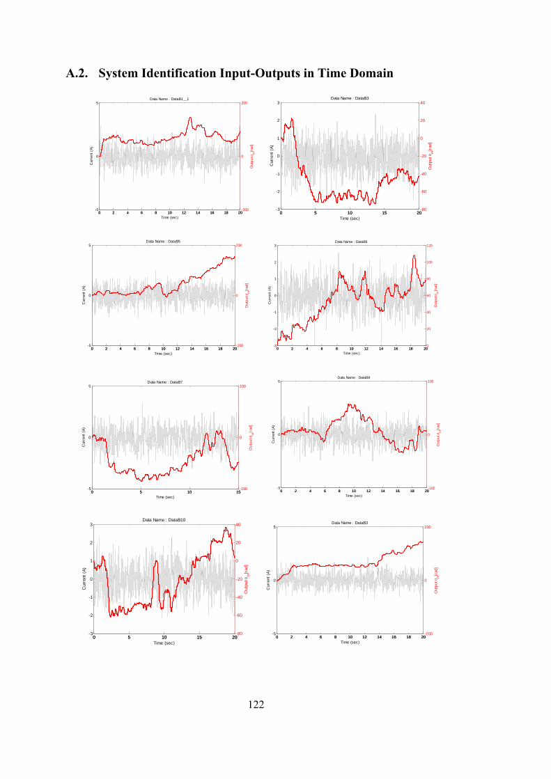
122
A.2. System Identification Input-Outputs in Time Domain
0 2 4 6 8 10 12 14 16 18 20-5
0
5
Cur
rent
(A
)
Data Name : DataB1__1
0 2 4 6 8 10 12 14 16 18 20-200
0
200
Out
pu
t m
[rad
]
Time (sec)0 5 10 15 20
-3
-2
-1
0
1
2
3
Cur
rent
(A
)
Data Name : DataB3
0 5 10 15 20-80
-60
-40
-20
0
20
40
Out
put
m[r
ad]
Time (sec)
0 2 4 6 8 10 12 14 16 18 20-5
0
5
Cur
rent
(A
)
Data Name : DataB5
0 2 4 6 8 10 12 14 16 18 20-200
0
200O
utp
ut
m[r
ad]
Time (sec)0 2 4 6 8 10 12 14 16 18 20
-3
-2
-1
0
1
2
3
Cur
rent
(A
)
Data Name : DataB6
0 2 4 6 8 10 12 14 16 18 200
20
40
60
80
100
120
Out
pu
t m
[rad
]
Time (sec)
0 5 10 15-5
0
5
Cur
rent
(A
)
Data Name : DataB7
0 5 10 15-100
0
100
Out
put
m[r
ad]
Time (sec)
0 2 4 6 8 10 12 14 16 18 20-5
0
5
Cur
rent
(A
)
Data Name : DataB9
0 2 4 6 8 10 12 14 16 18 20-100
0
100
Out
put
m[r
ad]
Time (sec)
0 5 10 15 20-3
-2
-1
0
1
2
3
Cur
rent
(A
)
Data Name : DataB10
0 5 10 15 20-80
-60
-40
-20
0
20
40
Out
pu
t m
[rad
]
Time (sec)0 2 4 6 8 10 12 14 16 18 20
-5
0
5
Cur
rent
(A
)
Data Name : DataB3
0 2 4 6 8 10 12 14 16 18 20-200
0
200
Out
put
m[r
ad]
Time (sec)
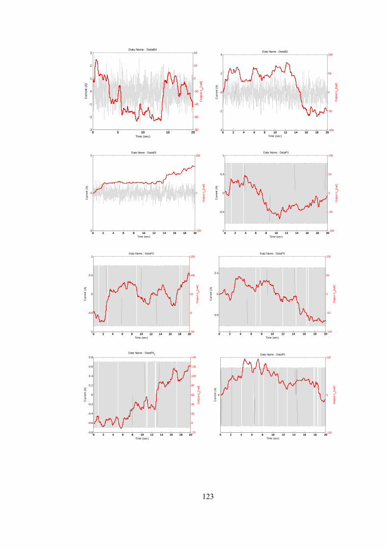
123
0 5 10 15 20-3
-2
-1
0
1
2
3
Cur
rent
(A
)
Data Name : DataB4
0 5 10 15 20-80
-60
-40
-20
0
20
40
Out
pu
t m
[rad
]
Time (sec)0 2 4 6 8 10 12 14 16 18 20
-4
-2
0
2
4
Cur
rent
(A
)
Data Name : DataB2
0 2 4 6 8 10 12 14 16 18 20-100
-50
0
50
100
Out
pu
t m
[rad
]
Time (sec)
0 2 4 6 8 10 12 14 16 18 20-5
0
5
Cur
rent
(A
)
Data Name : DataB3
0 2 4 6 8 10 12 14 16 18 20-200
0
200
Out
put
m[r
ad]
Time (sec)0 2 4 6 8 10 12 14 16 18 20
-1
-0.5
0
0.5
1
Cur
rent
(A
)
Data Name : DataP1
0 2 4 6 8 10 12 14 16 18 20-100
-50
0
50
100
Out
put
m[r
ad]
Time (sec)
0 2 4 6 8 10 12 14 16 18 20-1
-0.5
0
0.5
1
Cur
rent
(A
)
Data Name : DataP2
0 2 4 6 8 10 12 14 16 18 20-50
0
50
100
150
Out
pu
t m
[rad
]
Time (sec)0 2 4 6 8 10 12 14 16 18 20
-0.5
0
0.5
Data Name : DataP3
Cur
rent
(A
)
0 2 4 6 8 10 12 14 16 18 20-100
-50
0
50
100
Out
pu
t m
[rad
]Time (sec)
0 2 4 6 8 10 12 14 16 18 20-0.8
-0.6
-0.4
-0.2
0
0.2
0.4
0.6
0.8
Cur
rent
(A
)
Data Name : DataP41
0 2 4 6 8 10 12 14 16 18 20-20
0
20
40
60
80
100
120
140
Out
put
m[r
ad]
Time (sec)0 2 4 6 8 10 12 14 16 18 20
0
Cur
rent
(A
)
Data Name : DataP5
0 2 4 6 8 10 12 14 16 18 20-100
0
100
Out
pu
t m
[rad
]
Time (sec)
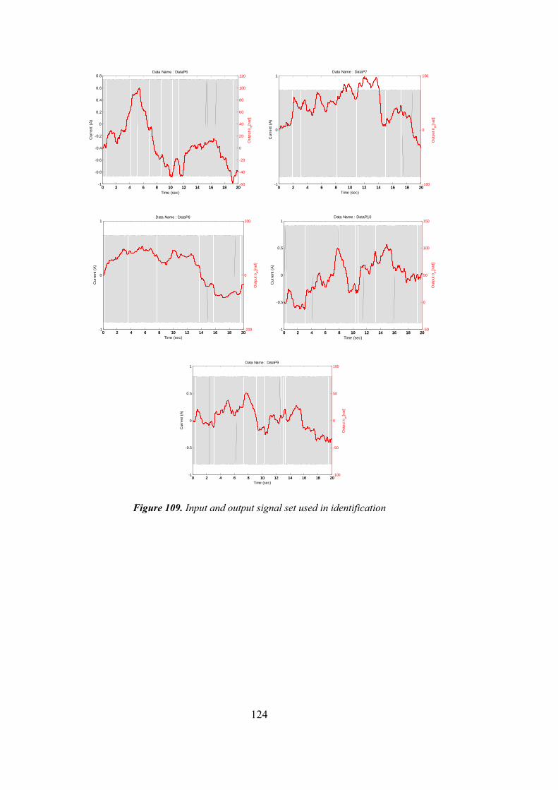
124
Figure 109. Input and output signal set used in identification
0 2 4 6 8 10 12 14 16 18 20-1
-0.8
-0.6
-0.4
-0.2
0
0.2
0.4
0.6
0.8
Cur
rent
(A
)
Data Name : DataP6
0 2 4 6 8 10 12 14 16 18 20-60
-40
-20
0
20
40
60
80
100
120
Out
pu
t m
[rad
]
Time (sec)0 2 4 6 8 10 12 14 16 18 20
-1
0
1
Cur
rent
(A
)
Data Name : DataP7
0 2 4 6 8 10 12 14 16 18 20-100
0
100
Out
put
m[r
ad]
Time (sec)
0 2 4 6 8 10 12 14 16 18 20-1
0
1
Cur
rent
(A
)
Data Name : DataP8
0 2 4 6 8 10 12 14 16 18 20-200
0
200
Out
pu
t m
[rad
]
Time (sec)0 2 4 6 8 10 12 14 16 18 20
-1
-0.5
0
0.5
1
Cur
rent
(A
)
Data Name : DataP10
0 2 4 6 8 10 12 14 16 18 20-50
0
50
100
150
Out
pu
t m
[rad
]
Time (sec)
0 2 4 6 8 10 12 14 16 18 20-1
-0.5
0
0.5
1
Cur
rent
(A
)
Data Name : DataP9
0 2 4 6 8 10 12 14 16 18 20-100
-50
0
50
100
Out
pu
t m
[rad
]
Time (sec)
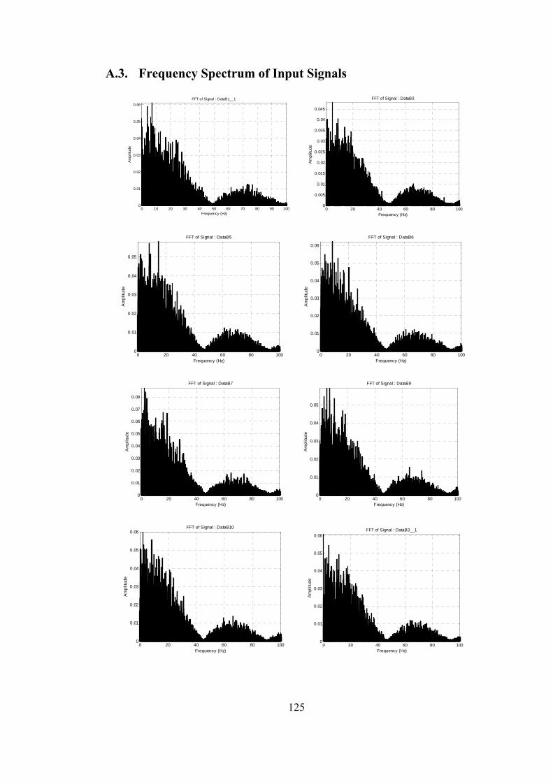
125
A.3. Frequency Spectrum of Input Signals
0 10 20 30 40 50 60 70 80 90 1000
0.01
0.02
0.03
0.04
0.05
0.06
FFT of Signal : DataB1__1
Frequency (Hz)
Am
plit
ude
0 20 40 60 80 1000
0.005
0.01
0.015
0.02
0.025
0.03
0.035
0.04
0.045
Frequency (Hz)
Am
plit
ude
FFT of Signal : DataB3
0 20 40 60 80 1000
0.01
0.02
0.03
0.04
0.05
Frequency (Hz)
Am
plit
ud
e
FFT of Signal : DataB5
0 20 40 60 80 1000
0.01
0.02
0.03
0.04
0.05
0.06
Frequency (Hz)
Am
plit
ud
e
FFT of Signal : DataB6
0 20 40 60 80 1000
0.01
0.02
0.03
0.04
0.05
0.06
0.07
0.08
Frequency (Hz)
Am
plit
ud
e
FFT of Signal : DataB7
0 20 40 60 80 1000
0.01
0.02
0.03
0.04
0.05
Frequency (Hz)
Am
plit
ud
e
FFT of Signal : DataB9
0 20 40 60 80 1000
0.01
0.02
0.03
0.04
0.05
0.06
Frequency (Hz)
Am
plit
ud
e
FFT of Signal : DataB10
0 20 40 60 80 1000
0.01
0.02
0.03
0.04
0.05
0.06
Frequency (Hz)
Am
plit
ude
FFT of Signal : DataB3__1
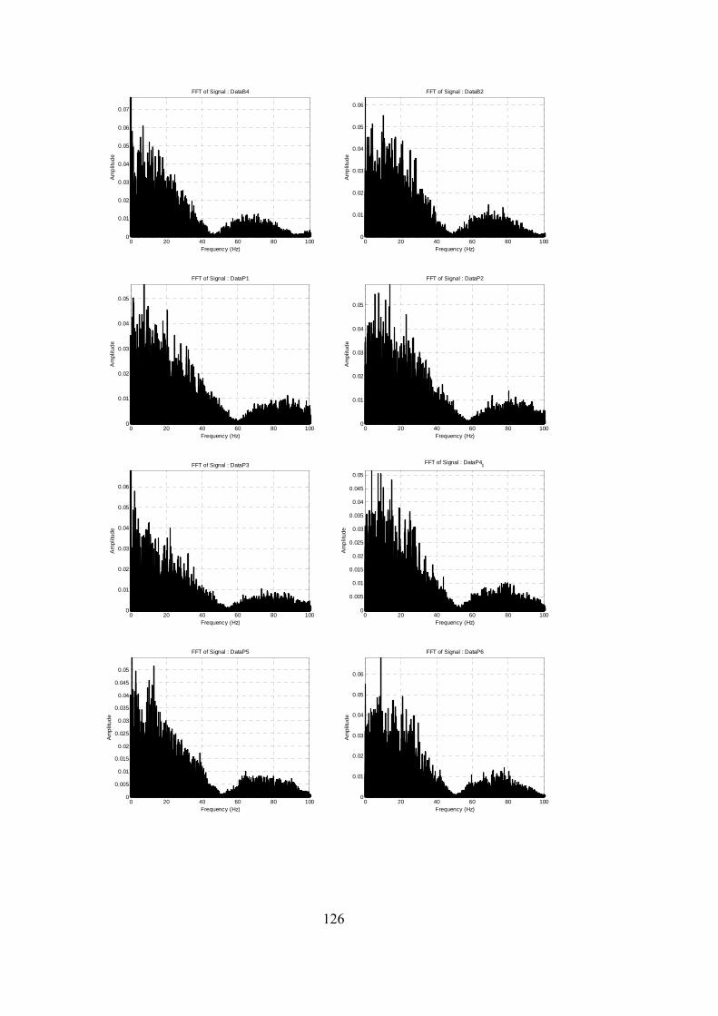
126
0 20 40 60 80 1000
0.01
0.02
0.03
0.04
0.05
0.06
0.07
Frequency (Hz)
Am
plit
ud
e
FFT of Signal : DataB4
0 20 40 60 80 1000
0.01
0.02
0.03
0.04
0.05
0.06
Frequency (Hz)
Am
plit
ud
e
FFT of Signal : DataB2
0 20 40 60 80 1000
0.01
0.02
0.03
0.04
0.05
Frequency (Hz)
Am
plit
ud
e
FFT of Signal : DataP1
0 20 40 60 80 1000
0.01
0.02
0.03
0.04
0.05
Frequency (Hz)
Am
plit
ud
e
FFT of Signal : DataP2
0 20 40 60 80 1000
0.01
0.02
0.03
0.04
0.05
0.06
Frequency (Hz)
Am
plit
ud
e
FFT of Signal : DataP3
0 20 40 60 80 1000
0.005
0.01
0.015
0.02
0.025
0.03
0.035
0.04
0.045
0.05
Frequency (Hz)
Am
plit
ud
e
FFT of Signal : DataP41
0 20 40 60 80 1000
0.005
0.01
0.015
0.02
0.025
0.03
0.035
0.04
0.045
0.05
Frequency (Hz)
Am
plit
ud
e
FFT of Signal : DataP5
0 20 40 60 80 1000
0.01
0.02
0.03
0.04
0.05
0.06
Frequency (Hz)
Am
plit
ud
e
FFT of Signal : DataP6
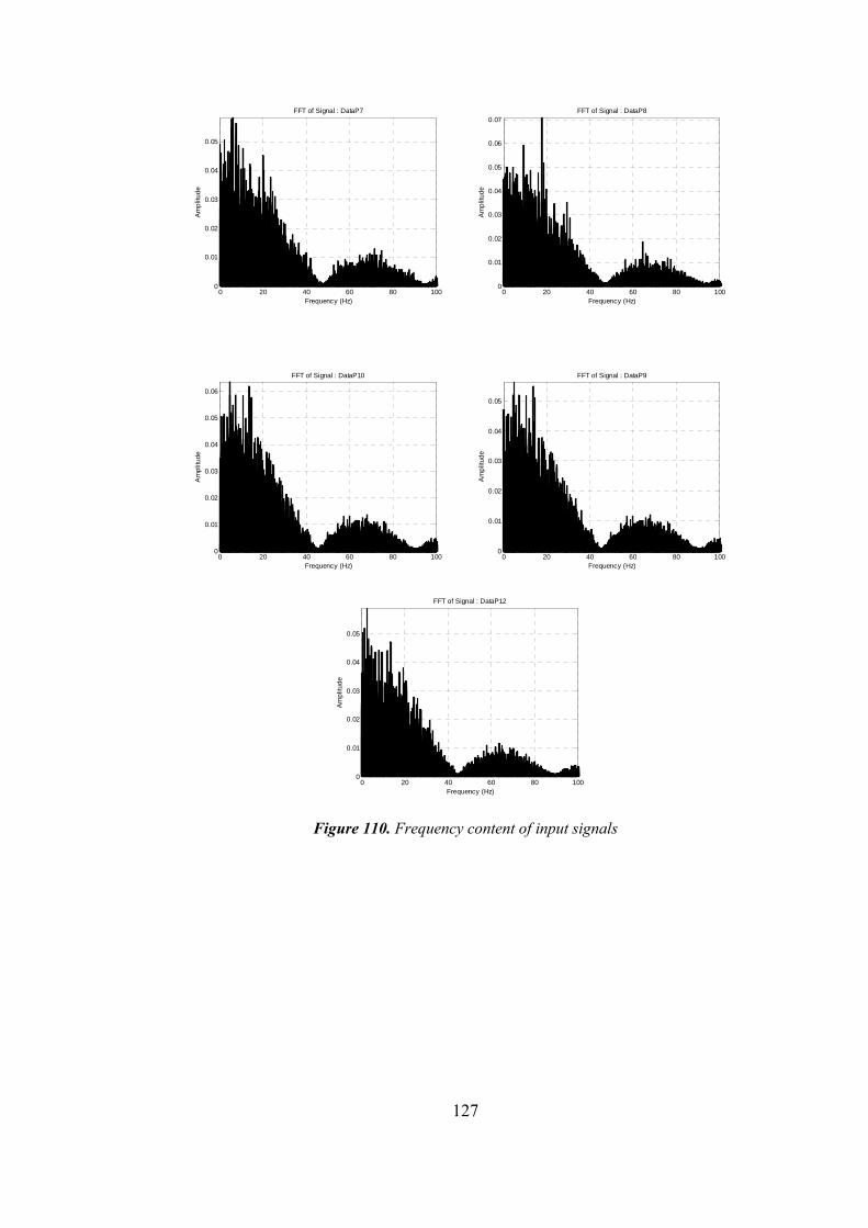
127
Figure 110. Frequency content of input signals
0 20 40 60 80 1000
0.01
0.02
0.03
0.04
0.05
Frequency (Hz)
Am
plit
ud
e
FFT of Signal : DataP7
0 20 40 60 80 1000
0.01
0.02
0.03
0.04
0.05
0.06
0.07
Frequency (Hz)
Am
plit
ud
e
FFT of Signal : DataP8
0 20 40 60 80 1000
0.01
0.02
0.03
0.04
0.05
0.06
Frequency (Hz)
Am
plit
ud
e
FFT of Signal : DataP10
0 20 40 60 80 1000
0.01
0.02
0.03
0.04
0.05
Frequency (Hz)
Am
plit
ud
e
FFT of Signal : DataP9
0 20 40 60 80 1000
0.01
0.02
0.03
0.04
0.05
Frequency (Hz)
Am
plit
ud
e
FFT of Signal : DataP12
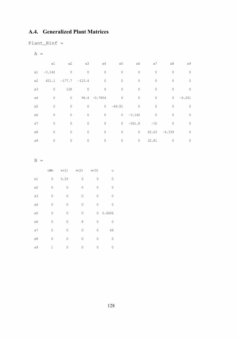
128
A.4. Generalized Plant Matrices
Plant_Hinf =
A =
x1 x2 x3 x4 x5 x6 x7 x8 x9
x1 -3.142 0 0 0 0 0 0 0 0
x2 421.1 -177.7 -123.4 0 0 0 0 0 0
x3 0 128 0 0 0 0 0 0 0
x4 0 0 96.4 -0.7854 0 0 0 0 -6.251
x5 0 0 0 0 -69.81 0 0 0 0
x6 0 0 0 0 0 -3.142 0 0 0
x7 0 0 0 0 0 -261.8 -10 0 0
x8 0 0 0 0 0 0 65.63 -6.339 0
x9 0 0 0 0 0 0 32.81 0 0
B =
uWm w(1) w(2) w(3) u
x1 0 0.25 0 0 0
x2 0 0 0 0 0
x3 0 0 0 0 0
x4 0 0 0 0 0
x5 0 0 0 0 0.6606
x6 0 0 8 0 0
x7 0 0 0 0 64
x8 0 0 0 0 0
x9 1 0 0 0 0
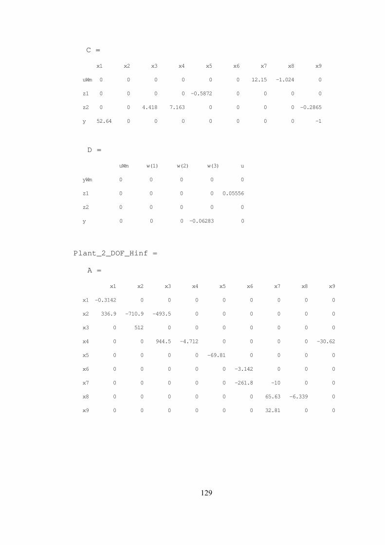
129
C =
x1 x2 x3 x4 x5 x6 x7 x8 x9
uWm 0 0 0 0 0 0 12.15 -1.024 0
z1 0 0 0 0 -0.5872 0 0 0 0
z2 0 0 4.418 7.163 0 0 0 0 -0.2865
y 52.64 0 0 0 0 0 0 0 -1
D =
uWm w(1) w(2) w(3) u
yWm 0 0 0 0 0
z1 0 0 0 0 0.05556
z2 0 0 0 0 0
y 0 0 0 -0.06283 0
Plant_2_DOF_Hinf =
A =
x1 x2 x3 x4 x5 x6 x7 x8 x9
x1 -0.3142 0 0 0 0 0 0 0 0
x2 336.9 -710.9 -493.5 0 0 0 0 0 0
x3 0 512 0 0 0 0 0 0 0
x4 0 0 944.5 -4.712 0 0 0 0 -30.62
x5 0 0 0 0 -69.81 0 0 0 0
x6 0 0 0 0 0 -3.142 0 0 0
x7 0 0 0 0 0 -261.8 -10 0 0
x8 0 0 0 0 0 0 65.63 -6.339 0
x9 0 0 0 0 0 0 32.81 0 0
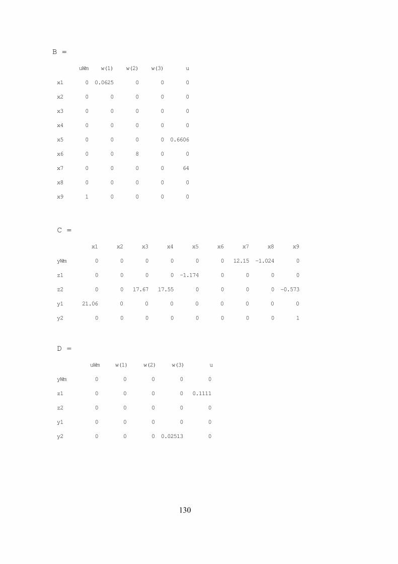
130
B =
uWm w(1) w(2) w(3) u
x1 0 0.0625 0 0 0
x2 0 0 0 0 0
x3 0 0 0 0 0
x4 0 0 0 0 0
x5 0 0 0 0 0.6606
x6 0 0 8 0 0
x7 0 0 0 0 64
x8 0 0 0 0 0
x9 1 0 0 0 0
C =
x1 x2 x3 x4 x5 x6 x7 x8 x9
yWm 0 0 0 0 0 0 12.15 -1.024 0
z1 0 0 0 0 -1.174 0 0 0 0
z2 0 0 17.67 17.55 0 0 0 0 -0.573
y1 21.06 0 0 0 0 0 0 0 0
y2 0 0 0 0 0 0 0 0 1
D =
uWm w(1) w(2) w(3) u
yWm 0 0 0 0 0
z1 0 0 0 0 0.1111
z2 0 0 0 0 0
y1 0 0 0 0 0
y2 0 0 0 0.02513 0
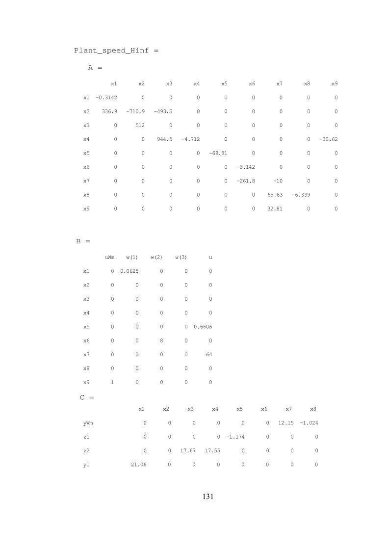
131
Plant_speed_Hinf =
A =
x1 x2 x3 x4 x5 x6 x7 x8 x9
x1 -0.3142 0 0 0 0 0 0 0 0
x2 336.9 -710.9 -493.5 0 0 0 0 0 0
x3 0 512 0 0 0 0 0 0 0
x4 0 0 944.5 -4.712 0 0 0 0 -30.62
x5 0 0 0 0 -69.81 0 0 0 0
x6 0 0 0 0 0 -3.142 0 0 0
x7 0 0 0 0 0 -261.8 -10 0 0
x8 0 0 0 0 0 0 65.63 -6.339 0
x9 0 0 0 0 0 0 32.81 0 0
B =
uWm w(1) w(2) w(3) u
x1 0 0.0625 0 0 0
x2 0 0 0 0 0
x3 0 0 0 0 0
x4 0 0 0 0 0
x5 0 0 0 0 0.6606
x6 0 0 8 0 0
x7 0 0 0 0 64
x8 0 0 0 0 0
x9 1 0 0 0 0
C =
x1 x2 x3 x4 x5 x6 x7 x8
yWm 0 0 0 0 0 0 12.15 -1.024
z1 0 0 0 0 -1.174 0 0 0
z2 0 0 17.67 17.55 0 0 0 0
y1 21.06 0 0 0 0 0 0 0

132
y2 0 0 0 0 0 0 0 0
x9
yWm 0
z1 0
z2 -0.573
y1 0
y2 1
D =
uWm w(1) w(2) w(3) u
yWm 0 0 0 0 0
z1 0 0 0 0 0.1111
z2 0 0 0 0 0
y1 0 0 0 0 0
y2 0 0 0 0.02513 0
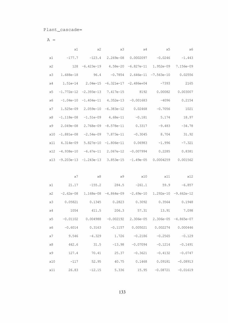
133
Plant_cascade=
A =
x1 x2 x3 x4 x5 x6
x1 -177.7 -123.4 2.269e-08 0.0002097 -0.0246 -1.443
x2 128 -6.423e-19 4.58e-20 -6.827e-11 1.952e-09 7.156e-09
x3 1.688e-18 96.4 -0.7854 2.646e-11 -7.563e-10 0.02556
x4 1.51e-14 2.04e-15 -6.321e-17 -2.486e+04 -7393 2165
x5 -1.772e-12 -2.393e-13 7.417e-15 8192 0.00082 0.003007
x6 -1.04e-10 -1.404e-11 4.352e-13 -0.001683 -4096 0.2154
x7 1.525e-09 2.059e-10 -6.383e-12 0.02468 -0.7056 1021
x8 -1.118e-08 -1.51e-09 4.68e-11 -0.181 5.174 18.97
x9 2.049e-08 2.768e-09 -8.578e-11 0.3317 -9.483 -34.78
x10 -1.881e-08 -2.54e-09 7.873e-11 -0.3045 8.704 31.92
x11 4.314e-09 5.827e-10 -1.806e-11 0.06983 -1.996 -7.321
x12 -4.938e-10 -6.67e-11 2.067e-12 -0.007994 0.2285 0.8381
x13 -9.203e-13 -1.243e-13 3.853e-15 -1.49e-05 0.0004259 0.001562
x7 x8 x9 x10 x11 x12
x1 21.17 -155.2 284.5 -261.1 59.9 -6.857
x2 -2.62e-08 1.168e-08 -4.864e-09 -2.69e-10 1.292e-10 -9.662e-12
x3 0.05821 0.1345 0.2823 0.3092 0.3564 0.1948
x4 1054 411.5 206.3 57.31 13.91 7.098
x5 -0.01102 0.004988 -0.002192 2.306e-05 2.306e-05 -4.865e-07
x6 -0.6014 0.3163 -0.1157 0.005021 0.002274 0.000446
x7 9.546 -4.329 1.726 -0.2186 -0.2565 -0.129
x8 442.6 31.5 -13.98 -0.07094 -0.1214 -0.1491
x9 127.4 70.41 25.37 -0.3621 -0.4132 -0.0747
x10 -117 52.95 40.75 0.1468 0.09181 -0.08913
x11 26.83 -12.15 5.336 15.95 -0.08721 -0.01619
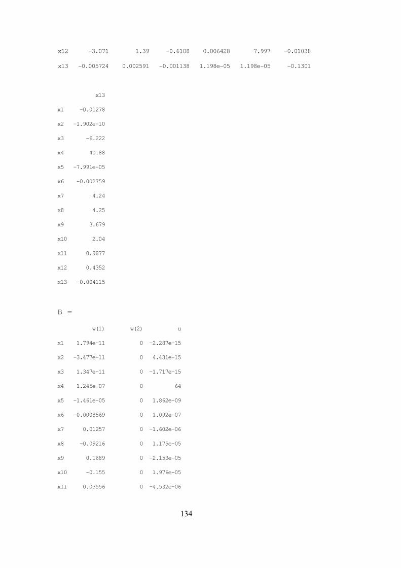
134
x12 -3.071 1.39 -0.6108 0.006428 7.997 -0.01038
x13 -0.005724 0.002591 -0.001138 1.198e-05 1.198e-05 -0.1301
x13
x1 -0.01278
x2 -1.902e-10
x3 -6.222
x4 40.88
x5 -7.991e-05
x6 -0.002759
x7 4.24
x8 4.25
x9 3.679
x10 2.04
x11 0.9877
x12 0.4352
x13 -0.004115
B =
w(1) w(2) u
x1 1.794e-11 0 -2.287e-15
x2 -3.477e-11 0 4.431e-15
x3 1.347e-11 0 -1.717e-15
x4 1.245e-07 0 64
x5 -1.461e-05 0 1.862e-09
x6 -0.0008569 0 1.092e-07
x7 0.01257 0 -1.602e-06
x8 -0.09216 0 1.175e-05
x9 0.1689 0 -2.153e-05
x10 -0.155 0 1.976e-05
x11 0.03556 0 -4.532e-06
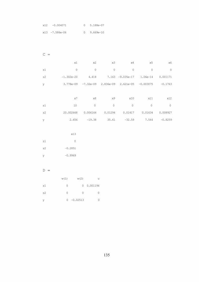
135
x12 -0.004071 0 5.188e-07
x13 -7.586e-06 0 9.669e-10
C =
x1 x2 x3 x4 x5 x6
z1 0 0 0 0 0 0
z2 -1.302e-20 4.418 7.163 -9.035e-17 1.06e-14 0.001171
y 3.778e-09 -7.32e-09 2.836e-09 2.621e-05 -0.003075 -0.1763
x7 x8 x9 x10 x11 x12
z1 10 0 0 0 0 0
z2 20.002668 0.006164 0.01294 0.01417 0.01634 0.008927
y 2.656 -19.38 35.61 -32.59 7.544 -0.8259
x13
z1 0
z2 -0.2851
y -0.9969
D =
w(1) w(2) u
z1 0 0 0.001194
z2 0 0 0
y 0 -0.02513 0

136
A.5. Weightings Functions of Cascade H∞ Controller
H∞ Speed Controller
0.4363
0.2122 1refWs
30
0.3183 1hingeWs
0.055556 17.4557
349.1u
sW
s
2
2 2, 100 , 2 / 2
2n
ideal nn n
W Hzs s
0.057296 18.0024
15.71perf
sW
s
2 2 / 500noiseW pi
H∞ Position Controller
0.01745
0.3138 1refWs
30
0.3183 1hingeWs
1
200*240* /180uWpi
2
2 2, 20 , 2 / 2
2n
ideal nn n
W Hzs s
0.28648 90.0120
15.71perf
sW
s
2 2 / 500noiseW pi