Version 1.03 1

Dynamic Line Integral Convolution: A Guide to the Java Software

NOTE: Many of the links in this document will only work if you have installed this pdf

file in the location described in Section 3.1 below.

IN PDF FORMAT THIS DOCUMENT HAS BOOKMARKS FOR NAVIGATION

CLICK ON THE UPPER LEFT “BOOKMARK” TAB IN THE PDF READER

Version 1.03 December 22, 2007

Software and Documentation: Andreas Sundquist Additional Software and Documentation: John Belcher, Michael Danziger

Copyright © 2007 Andreas Sundquist. This work is licensed under a Creative Commons

Attribution 2.5 License.

Comments and questions to jbelcher@mit.edu

Version 1.03 2

Table of Contents (LIVE LINKS)

1 Introduction................................................................................................................. 5

1.1 Motivation........................................................................................................... 5 1.2 What’s New in Release 1.01? ............................................................................. 5 1.3 What’s New in Release 1.02? ............................................................................. 6 1.4 What’s New in Release 1.03? ............................................................................. 6

2 What is a DLIC? ......................................................................................................... 6 2.1 LIC ...................................................................................................................... 6 2.2 DLIC ................................................................................................................... 9 2.3 The Falling Ring ............................................................................................... 10

3 Setting Up the SundquistDLIC Project ..................................................................... 11 3.1 Downloading and Installing the DLIC Java Code Base and Documentation ... 11 3.2 Installing Java and Eclipse in a Windows Environment .................................. 11 3.3 Creating a SundquistDLIC Java Project in Eclipse........................................... 12 3.4 The Package Structure of the SundquistDLIC Java Project.............................. 13

3.4.1 core............................................................................................................ 14 3.4.2 doc............................................................................................................. 15 3.4.3 simulations ................................................................................................ 15 3.4.4 DLICdoc ................................................................................................... 15

4 Examples of DLIC Generation ................................................................................. 17 4.1 Overview........................................................................................................... 17 4.2 The Falling Ring ............................................................................................... 17 4.3 Electrostatics ..................................................................................................... 19 4.4 Magnetostatics .................................................................................................. 20 4.5 The Oscillating Radiating Dipole ..................................................................... 21 4.6 Fluid Flow......................................................................................................... 22

4.6.1 Fluid Flow from Analytic Functions......................................................... 22 4.6.2 Fluid Flow Speed Varying With Region in an Image............................... 23 4.6.3 Fluid Flow from Data Input ...................................................................... 24

4.7 Running an Animation...................................................................................... 24 5 Postprocessing........................................................................................................... 26

5.1 Making a Sequence of Images Periodic............................................................ 26 5.2 Color Coding..................................................................................................... 26

5.2.1 The HSV Scale (after http://en.wikipedia.org/wiki/HSV_color_space)... 27 5.2.2 Color Mode 0 ............................................................................................ 27 5.2.3 Color Mode 1 ............................................................................................ 27 5.2.4 Color Mode 2 ............................................................................................ 28 5.2.5 Color Mode 3 ............................................................................................ 29 5.2.6 Color Mode 4 ............................................................................................ 29

5.3 Rendering a Single Large Image in a Sequence ............................................... 30 6 Incorporating a Sequence of DLIC Images into a 3ds max Scene............................ 31

6.1 Creating a 3ds max Scene with Animated Objects and a Screen...................... 31 6.2 Projecting the DLIC on the Screen in the 3ds max Scene ................................ 33

7 References................................................................................................................. 36

Version 1.03 3

8 Index ......................................................................................................................... 37

Version 1.03 4

Figure Captions Figure 2.1-1: To produce a LIC image for the constant field F, we take each pixel in a

random pattern, for example, pixel 1, and average the brightness of the n pixels lying along a line parallel to F centered on pixel 1, as indicated by the while line............... 7

Figure 2.1-2: We calculate the brightness at pixels 2 and 3 by averaging over the brightness of the n pixels lying along the lines parallel to F centered on pixels 2 and 3, as indicated by the two white lines........................................................................... 7

Figure 2.1-3: A LIC of a constant field, constructed in the manner described in the text. 8 Figure 2.1-4: LIC for a Faraday’s Law visualization. A conducting ring is falls toward a

stationary magnetic dipole, and eddy currents are induced in the ring. ....................... 9 Figure 3.1-1: Setting the default .java application reader to Notepad ............................. 11 Figure 3.3-1: The Package Structure of the SundquistDLIC Project ............................... 13 Figure 4.2-1: One Image Generated by the Falling Ring Animation, after insertion in to

3ds max 2008 file. ...................................................................................................... 19 Figure 4.3-1: One frame of the RepulsionTwoCharges Animation................................. 20 Figure 4.6-1: An Example of a Fluid Flow Image........................................................... 23 Figure 4.6-2: Fluid Flow Varying According To Region ................................................ 24 Figure 4.7-1: Running an Animation ............................................................................... 25 Figure 4.7-2: The Run dialog box.................................................................................... 25 Figure 4.7-3: Increasing the Memory in Eclipse ............................................................. 26 Figure 5.2-1: HSV............................................................................................................ 27 Figure 5.2-2: Color Mode 1 ............................................................................................. 28 Figure 5.2-3: Color Mode 2 with S and V values. ........................................................... 28 Figure 5.2-4: An example of the usefulness of Color Mode............................................ 29 Figure 5.2-5: Coloring of a DLIC by region.................................................................... 30 Figure 6.1-1: The upper right of the 3ds max main interface ........................................... 31 Figure 6.1-2: The Utilities panel after selecting MAXScript ........................................... 32 Figure 6.1-3: The Open Script dialog box ....................................................................... 32 Figure 6.1-4 : The Editor Window for MAX script files. ................................................. 33 Figure 6.2-1: The Material Editor window. .................................................................... 34 Figure 6.2-2: The Material/Map Browser window.......................................................... 34 Figure 6.2-3: The Select Bitmap Image File window...................................................... 35 Figure 6.2-4: The Material Editor Icons after assigning the DLIC files .......................... 35

Version 1.03 5

1 Introduction 1.1 Motivation

The visualization of time dependent vector fields is a central problem in scientific

visualization. There have been two advances in computer graphics since 1993 which have fundamentally changed the way that vector fields can be visualized in two dimensions. The first of these was the introduction of the Line Integral Convolution (LIC) method for showing the structure of vector fields at a resolution near that of the display, using textures generated by convolving the vector field with a grid of pixels of random brightness [Cabral and Leedom, 1993].

The second was the introduction of a method for the animation of a LIC using a

second velocity field to evolve the underlying grid of random pixels used to generate the LIC [Sundquist, 2001; Sundquist, 2003]. Links to these papers may be found at 2001 and at 2003. This latter method, called Dynamic Line Integral Convolution (DLIC), produces an animated sequence of images of the first field such that the time dependence of that field is evident from frame to frame by the inter-frame coherence in the LIC texture pattern. We discuss more details of this process below in Section 2.

In a paper to be submitted to the American Journal of Physics, Belcher and Koleci

[2007] discuss at a heuristic level how these two algorithms work, and why they are effective learning tools for electromagnetism. The motivation for this paper is to make the LIC and DLIC methods and their educational impact more widely known to the physics community.

The present document first gives a brief heuristic discussion of what a DLIC is. Then, starting with Section 3, we provide a guide to the software code developed by Andreas Sundquist to produce DLICs. Assembling the documentation has been carried out by John Belcher, and additional programming has been provided by Michael Danziger and John Belcher. Our intended audience is undergraduates, graduate students or postdoctoral fellows in science and engineering who have some knowledge of programming who would like to produce DLICs for applications in their specialty. This is a set of instructions and examples that will enable someone with that background to create DLICs.

1.2 What’s New in Release 1.01? Compared to release 1.0, we have added extensive documentation about adding color to the DLIC, and we have changed the definition of the color modes so that we have more flexibility in adding color. We have moved the Colorizer method into its own separate class. We have added more examples of using the program for electromagnetism.

Version 1.03 6

1.3 What’s New in Release 1.02? Compared to release 1.01, we have added ColorMode 4. This mode allows the user to color the image by region, as opposed to flat color or a color linked to field strength (see Section 5.2.6). We have also added a new mode for showing fluid flow, in which the flow speed varies by region as opposed to remaining constant across the image or varying with field strength (see Section 4.6.2). We have added an additional paper using the DLIC method to our paper collection located at this link (Liu and Belcher 2007), and we have included the classes used to make the figures in that paper. 1.4 What’s New in Release 1.03? Compared to release 1.02, we have added a new feature that allows one to set the origin of the DLIC as different from zero if you have no symmetry in the DLIC. This feature is described in Section 3.4.1.7 below. We have added to our animation classes code to animate the electric field of a linear antenna.

2 What is a DLIC? 2.1 LIC The LIC method uses correlations in a texture pattern to show the spatial structure of a vector field. To explain heuristically how the LIC algorithm works, we first consider a constant field. Given a square array of NxN pixels of random brightness, we want to generate a textured array of the same dimension, where the texture pattern indicates the direction of the constant field, to within a sign. To do this, we process our NxN random array pixel by pixel to produce the new texture array, as follows. At any pixel 1 (see Figure 2.1-1), we average the brightness of the pixels along a line centered on pixel 1 and in the direction of the local field, for n pixels, n << N, and put this value in our new texture array at the same location as pixel 1 was in the initial array. We now move to an adjacent new pixel and repeat this same process again (Figure 2.1-2). If we move parallel to the field to get to the new pixel, say pixel 2 in Figure 2.1-2, then the resulting average that we obtain at pixel 2 is almost the same as the average for pixel 1, because most of the pixels are the same. So the calculated brightness at pixel 2 is highly correlated with the brightness of pixel 1. If on the other hand we move perpendicular to the field to get to the new pixel, say pixel 3 in Figure 2-1.2, the resulting average is not correlated at all with the average at pixel 1, because none of the pixels whose brightness is being averaged are the same. This process produces a new array which has correlations in brightness along the field direction. Another way of saying this is that we have produced a texture pattern where the streaks in the texture are parallel to the field direction, as shown in Figure 2.1-3.

Version 1.03 7

Figure 2.1-1: To produce a LIC image for the constant field F, we take each pixel in a random pattern, for example, pixel 1, and average the brightness of the n pixels lying along a line parallel to F centered on pixel 1, as indicated by the while line.

Figure 2.1-2: We calculate the brightness at pixels 2 and 3 by averaging over the brightness of the n pixels lying along the lines parallel to F centered on pixels 2 and

3, as indicated by the two white lines.

Version 1.03 8

Figure 2.1-3: A LIC of a constant field, constructed in the manner described in the text.

Now consider the LIC procedure for a field that varies in space. If we simply follow the procedure described above and average the brightness of pixels along straight lines in space, where the direction of the straight line is determined by the local direction of the field at (for example) pixel 1, we would get a visual representation of the field but it would be inaccurate, because we would be assuming that the local streamline can be reasonably approximated by a straight line along the entire n pixel averaging length. For locations where the local radius of curvature of a given field line is large compared to the n pixel length of the averaging line, this assumption is valid. However, if the local radius of curvature is comparable to or smaller than the length of n pixels along the averaging line, this assumption is no longer valid, and correlations in the texture pattern so generated will no longer show the details of structure of the field at this scale. To correct for this, the Cabral and Leedom LIC algorithm averages over n pixels along a line in space, but the averaging line is no longer a straight line, but the field line that passes through the point at which we are calculating the new texture value, for example pixel 1. That is, the texture pattern is convolved with the field structure along a line in space determined by the field lines, thus the name line integral convolution. This procedure retains the property that movement along the local field direction exhibits a high correlation in brightness values, but movement perpendicular to that direction exhibits little correlation, and this is true even in regions of high curvature. Figure 2.1-4 shows a LIC for the magnetic field of a conducting ring falling toward a stationary magnetic dipole (see also Section 2.3 and Section 4.2 below). Regions of high curvature occur near the two zeroes just above the ring. The zeroes are distinguishable by the tilted X-like structure near them. For comparison we also draw four field lines in the figure. We also note that although we mostly use the terminology LIC in what follows, the SundquistDLIC code actually uses a Fast Line Integral

Version 1.03 9

Convolution algorithm to compute the LIC, as introduced by Stalling and Hege 1995, and occasionally we will use the term FLIC.

Figure 2.1-4: LIC for a Faraday’s Law visualization. A conducting ring is falls toward a stationary magnetic dipole, and eddy currents are induced in the ring.

2.2 DLIC Dynamic Line Integral Convolution (DLIC) extends the LIC algorithm described above to time-dependent fields. The vector field F(x,t) is allowed to vary arbitrarily over time, with the motion of its field lines described by a second velocity vector field, D(x,t). That is, at any time t the field line of F(x,t) passing through x at time t is displaced in space at time t + Δt to a new position x + D(x,t) Δt. The DLIC algorithm originated by Sundquist produces an animation by evolving the random texture input used in LIC in a manner prescribed by the velocity field D. That is, if T(x,t) represents our random texture map, we evolve it with time according to

( ) ( )( ),T t t T t t t+ Δ = − Δx x D x, , (2.2.1)

Unfortunately, the texture is typically stored as a discrete array of values on an ordered grid. Repeatedly evolving that array over time will result in warping and a loss of detail. That is, the motion velocity field D may have divergent or convergent regions, which will spread out or compress the location of the pixels in our texture. To avoid this problem, instead of evolving the random input texture according to equation (1), the Sundquist DLIC algorithm tracks a large number of particles of random intensity, roughly on the same order as the number of pixels in the original input texture.

Version 1.03 10

The particles move over time with a velocity given by D, and the DLIC algorithm continuously monitors and adjusts their distribution to keep the level of detail roughly the same, by both consolidating old particles and creating new particles. At any instant of time for which we want to produce a frame of the animation, the texture at that time is generated by simply drawing all of the particles being followed onto it. Once we have the texture for a given frame, the LIC method is applied to this texture to render the image of the field at that time. Intuitively, since the particles that produce the input texture advect according to the motion field D, the LIC convolution of the field lines of F with the texture from one frame to the next samples the same part of the texture pattern, since the texture particles and field lines move in concert. Thus, the streaks in the LIC of F appear to move from one frame to the next according to the motion field D. Each output image in the sequence will individually have the same properties as a static LIC rendering, but successive frames will have an inter-frame coherence that depicts the prescribed motion of the field lines. 2.3 The Falling Ring We give an example of a situation in electromagnetism where the construction of a DLIC is of physical interest. A conducting ring with mass m, radius a, resistance R and self-inductance L is located on the z-axis above a stationary permanent magnet with magnetic dipole moment vector . The normal to the ring is along the vertical z-axis, and the ring is constrained to move along that axis. The ring is released from rest at t = 0, and falls under gravity toward the conducting ring. Eddy currents arise in the ring because of the changing magnetic flux as the magnet falls toward the ring, and the sense of these currents will be such as to slow the ring. The overall field configuration of the total magnetic field will be as shown in Figure 2.1-4. The solution for the motion of the ring involves the solution to three coupled ordinary differential equations for the z-coordinate of the falling ring, the current in the ring, and the z-coordinate of the velocity of the falling ring. These equations are given in Section 4.1 of the

zoM

TEAL_Physics_Math documentation. According the scheme introduced by Belcher and Olbert 2003 (linked at 2003) the magnetic field lines in this case should evolve with a velocity field given by

2B×

=E BD

(2.3.1)

The physical interpretation of this velocity field is that it represents the guiding center motion of a set of low energy electric monopoles initially arranged along any given magnetic field line, as those monopoles drift in the time-dependent electric and magnetic fields. We will return to this example in Section 4.2 below, where we discuss a specific example of the generation of a DLIC.

Version 1.03 11

3 Setting Up the SundquistDLIC Project 3.1 Downloading and Installing the DLIC Java Code Base and Documentation Go to http://web.mit.edu/viz/soft/ and follow links to the DLIC code base. You will download three zipped files, one under the link Source Code and named SundquistDLIC.zip, the second under the link DLIC Documentation and named DLICdoc.zip, and the third under the link General Documentation and named generalDoc.zip. Create a folder C:\Development\Projects\ on your C-drive and unzip SundquistDLIC.zip into the Projects folder. Unzip the DLICdoc.zip into the C:\Development\Projects\SundquistDLIC\ folder. Unzip the generalDoc.zip file into the C:\Development\Projects\ folder. Once you have done this you will have installed the DLIC code and documentation. All of the documentation discussed below is now contained in the two folders C:\Development\Projects\SundquistDLIC\DLICdoc and C:\Development\Projects\generalDoc. In particular this document in pdf format is contained in the folder DLICdoc. If you are not reading this document from that folder, many of the links will not work. In what follows we will provide links to the documentation on your C-drive assuming that you have installed the source code and documentation as described above. In particular when we discuss particular java files, we will link directly to those files. You may want to set the default application for reading .java files to Notepad. To do this, right click on any .java file, choose “Open With > Choose Program” from the dialog box (see Figure 1.2-1) and in the dialog box that then comes up, choose “Select the program from a list”. In the list that comes up, select Notepad and make sure you check the box labeled “Always use the selected program to open this kind of file”.

Figure 3.1-1: Setting the default .java application reader to Notepad

3.2 Installing Java and Eclipse in a Windows Environment

Version 1.03 12

We discuss the DLIC software in the context of Eclipse (http://www.eclipse.org/), a free, state-of-the-art Java Integrated Development Environment (IDE). We will assume that you are familiar with the Eclipse IDE interface, and developing Java applications in this environment. Step by step instructions for downloading Eclipse and the Java SDK (SDK stands for Software Development Kit) and creating a SundquistDLIC Java Project in Eclipse are given in a pdf file in your generalDoc folder at this link. To reiterate what active links in this document mean, “right-clicking” on the preceding link will take you to a pdf file named

InstallingJavaEclipseInWindows.pdf

in the folder C:\Development\Projects\generalDoc\. If you have downloaded and installed the code base and documentation in accord with the instructions in Section 3.1 above, the preceding link will open this document. We also provide a short document with common hints for using Eclipse, which explicitly tells you how to perform the various actions described below in Eclipse. This includes explanations for how to perform certain actions whose explanations are hard to find in the standard Help documentation on the Eclipse taskbar. That document in pdf format is at this link. 3.3 Creating a SundquistDLIC Java Project in Eclipse

Follow the directions in Section 3.2 in the pdf file at this link. When you have done this, open a Package Explorer window for the Project. You will see a directory tree for the packages in SundquistDLIC in Eclipse that looks like the one given on the next page in Figure 3.3-1.

Version 1.03 13

Figure 3.3-1: The Package Structure of the SundquistDLIC Project

3.4 The Package Structure of the SundquistDLIC Java Project To learn the structure of the DLIC package, the user should use this document as well as the javadocs and the actual java classes for the SundquistDLIC Project. We first give an overview of the package structure of the Project. This same information is included in the package documentation in the javadocs for the Project.

Version 1.03 14

3.4.1 core 3.4.1.1 core.dlic This package contains classes which create and evolve the individual FLIC images making up a movie of a given experiment. FLIC computes the Fast Line Integral Convolution at each step of the evolution of a given experiment. Streamline is used by FLIC to trace streamlines of the fields and compute equally spaced sample points along them. DLIC computes the overall evolution of the random input field according to the velocity field specified by the animation of the experiment. 3.4.1.2 core.field This package contains a number of classes used to create and manipulate the images generated for a given animation of an experiment as it evolves. Vec2 and Vec3 refer to two and three dimensional fields, respectively. 3.4.1.3 core.image This package creates and evolves the individual FLIC images making up a movie of a given experiment. FLIC computes the Fast Line Integral Convolution at each step of the evolution of a given experiment. Streamline is used by FLIC to trace streamlines of the fields and compute equally spaced sample points along them. DLIC computes the overall evolution of the random input field according to the velocity field specified by the animation of the experiment. 3.4.1.4 core.io This package creates and handles various input/output functions for the final images that are created, as well as the window used to display those images in real time to the user as the DFLIC images are produced. ImageIO is used to input and output the final images generated. OutputWindow manages the window used to display the images in real time as they are produced. 3.4.1.5 core.math This package contains a variety of classes which handle vector manipulations and the evolution of a given experiment as it evolves. For example, it provides integration schemes for integrating ODE’s that define the evolution of a given experiment. We also define various special functions here, such as those used to evaluate elliptic integrals.

3.4.1.6 core.postprocessing This package performs various operations on the images created by a given simulation of an experiment after the images are created by the classes in core.dflic. For

Version 1.03 15

example, we color those images, or we “periodify” a long sequence of images so that when they are looped the movie appears to repeat seamlessly.

3.4.1.7 core.rendering This package handles all the code that draws and evolves the DLIC and the experiment. Built in are several handlers for adjusting all of the rendering parameters that might conceivably need adjusting. These parameters are set in the animation of the experiment. We enumerate one of the features here. If you have no symmetry in the DLIC to be generated, you can change the origin of the DLIC from the default value to (0,0,0) by using renderer.SetOrigin(new Vec3(100.,100.,100.) in the animation setting up the animation.

3.4.2 doc The doc folder contains the javadocs for the Project, in html format. The main html link is the index.html link in doc. 3.4.3 simulations 3.4.3.1 simulations.animations This package animations for electrostatic, magnetostatic, Faraday’s Law, radiation, and fluid flow experiments. An animation class contains the main routine that is executed to produce a given sequence of DLIC images for an experiment. The animation sets up the experiment parameters and also the parameters that control how the images produced are created (e.g. size, color, and so on). 3.4.3.2 simulations.experiments This package contains all the experiments for the various electrostatic, magnetostatic, Faraday’s Law, radiation, and fluid flow experiments. An experiment class assembles the various electromagnetic objects needed and defines how they interact and evolve. All experiments extend BaseExperiment (javadoc, java), where here and in the future the links following a reverence to a java file link to the javadocs for that file and the .java file itself, respectively. 3.4.3.3 simulations.objects This package contains all the various electromagnetic objects that the experiments assemble for a given experiment. Each electromagnetic object must define how its electromagnetic fields are calculated. All objects extend BaseObject (javadoc, java). 3.4.4 DLICdoc

Version 1.03 16

The DLICdoc folder contains a variety of documentation files in pdf format, including this one.

Version 1.03 17

4 Examples of DLIC Generation 4.1 Overview An overview of the computational process for generating a DLIC is as follows. The main program is always contained as a method in one of the classes in simulations.animations. That animation program creates an instance of an experiment. All experiments are contained in one of the classes in simulations.experiments and they each extend BaseExperiment (javadoc, java). The animation program sets up the experiment parameters (for example, the time step between frames), and also the parameters that control how the images produced are created (e.g. size, color, and so on). An animation program also always creates an instance of a Renderer (javadocs, java) object. These links will only work if you have installed this pdf file in the locations described in Section 3.1 above. The Renderer object then creates an instance of the DLIC generation program to generate the images, using classes in core.dflic. An experiment assembles the various electromagnetic objects needed for a given experiment and defines how they interact. An electromagnetic object is always contained in one of the classes in simulations.objects, and each extends BaseObject (javadoc, java). Each object knows how to calculate the electromagnetic fields associated with that kind of object. All of the electromagnetic objects in a given experiment are assembled by that experiment into a collection of electromagnetic objects of class EMCollection (javadocs, java). This collection knows how to compute the total electromagnetic fields in the experiment by summing the electromagnetic fields of the objects which it contains. If necessary, the experiment also specifies the kind of integrator used to integrate the equations for the evolution of the system, and specifies what these equations are. Note that the evolution of the experiment may be specified by analytic functions, in which case no integrator is necessary. Finally, an experiment specifies what field is to be displayed (electric or magnetic) and how the velocity D field discussed in Section 2.2 is to be calculated. The calculation of the velocity field takes place in the class core.field.EMVec2Field (javadocs, java) according to the kind of flow field specified in the experiment by the parameter FieldMotionType. 4.2 The Falling Ring To make the above concrete, we use the example of the falling ring discussed in Section 2.3 above. The ring of current and the magnetic dipole are both formed from the CurrentRing class (javadocs, java). The CurrentRing class knows now to calculate the non-relativistic electric and magnetic fields of a moving ring of current with current I and time rate of change of current dI/dt. The magnetic field is just given by the usual expression for the magnetic field of a ring of current, and the electric field is given by the motional electric field − × plus the induction electric field associated with the time-changing magnetic field. These expressions can be found in Section 3.2.2 of the

v B

TEAL_Physics_Math documentation, which should be at the link given as long as the SundquistDLIC documentation has been installed in the manner described in Section 3.1 of the current document.

Version 1.03 18

The experiment class FallingRingExperiment (javadocs, java) creates an EMCollection (javadocs, java) object which consists of two current ring objects, one at rest at the origin (the “point dipole”) and one falling from above along the z-axis. The dimensionless equations describing the evolution of the z-coordinate of the falling ring, the current in that ring, and the z-coordinate of the velocity of the falling ring, are given in Section 4.1.3 of the TEAL_Physics_Math documentation. The method Motion (javadocs) computes the time derivatives of these three parameters, and is used by a fourth order Runge Kutta integration scheme (javadocs, java) to find the behavior of the system as a function of time. Note that the time involved in the integration to evolve the experiment is small compared to the image computation, and we usually take many more steps than we need to take, to insure accuracy (see the parameter numberSmallSteps in BaseExperiment). The animation class FallingRingAnimation (javadocs, java) instantiates a FallingRingExperiment object with the desired parameters for that object. If you execute the class as it exists in the download (see Section 4.7 below for instructions on executing the program), it will produce 130 images in the folder C:\DLICs\fallingRing You should generate these files because we use these as input to the Periodify class example discussed below in Section 5.1. The parameters alpha and beta for the generated sequence of images are set such that this is a superconducting ring which is light enough that it levitates above the magnet, and thus the motion is periodic. We have set the time step between frames such that the motion of the ring repeats every 100 frames. We explain why we generate 130 frames, which is 30 frames more than the 100 frames needed for the motion to repeat, in Section 5.1 below, which discusses making a sequence of DLIC images periodic. Finally, the experiment FallingRingExperiment (javadocs, java) sets its FieldType to Constants.FIELD_BFIELD (javadocs, java) and its FieldMotionType to Constants.FIELD_MOTION_BFIELD. This means that when the DLIC is generated it is displaying the magnetic field of this collection of two EM objects as the F field discussed in Section 2.2 above, and is using equation (2) for the velocity field D used to evolve that F field. We include in the documentation a movie of the DLICs generated above in various formats, which can be found here. The way in which these movies are generated is discussed in Section 6 below. Figure 4.2-1 shows one frame of that movie.

Version 1.03 19

Figure 4.2-1: One Image Generated by the Falling Ring Animation, after insertion in to 3ds max 2008 file.

4.3 Electrostatics We next consider an electro-quasi-static example. The animation class, which always contains the main method, is RepulsionTwoChargesAnimation (javadocs, java), which instantiates the experiment TwoChargesExperiment (javadocs, java). This experiment creates an EMCollecton which is the sum of the two base objects PointCharge (javadocs, java) and MovingPointCharge (javadocs, java). These two base objects know how to calculate the non-relativistic electric and magnetic fields of a stationary and moving charge. The electric field is just given by the usual expression for the electric field of a point charge, and the magnet field is given by the motional magnetic field . 2/ c×v E The experiment class TwoChargesExperiment (javadoc, java) instantiates the two point charge objects, one at rest at the origin and one free to move along the z-axis. The equations describing the evolution of the z-coordinate of the moving charge simply reflect the coulomb repulsion between the stationary and moving charge. The method Motion (javadocs) computes the time derivatives of the position and speed of the moving charge, and is used by the fourth order Runge Kutta integration scheme to find the behavior of the system as a function of time. The animation class RepulsionTwoChargesAnimation (javadocs, java) instantiates a TwoChargesExperiment object with the desired parameters for that object. If you execute the class as it exists in the download (see Section 4.7 below for instructions on executing the program), it will produce 100 images in the folder: C:\DLICs\charges

Version 1.03 20

Figure 4.3-1 shows one frame of the sequence which will be generated. Note that the frame is colored using the default hue for electric fields, 0.1 on a 0-1 scale. This hue can be changed, as discussed in Section 5.2 below.

Figure 4.3-1: One frame of the RepulsionTwoCharges Animation Finally, the experiment TwoChargesExperiment sets its FieldType to Constants.FIELD_EFIELD (javadocs, java) and its FieldMotionType to Constants.FIELD_MOTION_EFIELD. This means that when the DLIC is generated it is displaying the electric field of this collection of EM objects as the F field discussed in Section 2.2 above, and is using equation (4.3.1) below for the velocity field D used to evolve that F field (see Belcher and Olbert).

22c

E×

=E BD

(4.3.1) 4.4 Magnetostatics We next consider a magneto-quasi-static example. The experiment consists of two rings of current, one above the other. The top one represents the small magnet in the TeachSpin© (http://www.teachspin.com/) experiment, which is suspended from a spring and the bottom one represents the bottom current ring in the TeachSpin experiment. We set the current in that ring using an external power supply. In this experiment we assume that the external power supply drives a current in the bottom current ring I(t) that varies sinusoidally with time:

( ) sin( )oI t I tω= (4.4.1) We assume that this problem is purely magnetostatic—that is, we assume that is there is no current induced anywhere in this problem due to a changing magnetic flux through any ring--e.g. there are no induced electric fields or currents of importance. Thus the

Version 1.03 21

current in the bottom ring is given exactly by equation (4.4.1) and we need not worry about any induced currents either from the moving magnet above the ring or from the self inductance of the ring itself. Moreover, consider only frequencies such that the motion of the magnet due to the changing current in the bottom ring is very close to quasi-static, and the amplitude of that motion is small. That is, we set the driving angular frequency ω very low compared to the natural frequency of oscillation of the magnet on the spring from which it is suspended. In this case, the magnetic force on the dipole due to the current in the ring below simply results in a displacement of the magnet from its equilibrium position that is proportional to the magnetic force on the magnet. Thus this displacement is in phase with the current in the bottom ring. For the assumed small displacement, we can write an equation for the displacement of the magnet from equilibrium as follows:

( ) sin( )oz t z tω= (4.4.2)

In this case, we have an analytic expression for the evolution of the experiment in equations (4.4.1) and (4.4.2), and do not need to integrate any equations of motion. The animation class in this case, which always contains the main method, is TeachSpinAnimation (javadocs, java), which instantiates the experiment TeachSpinExperiment (javadocs, java). This experiment creates an EMCollecton which is the sum of two CurrentRing (javadocs, java) objects. These two base objects know how to calculate the non-relativistic electric and magnetic fields of a stationary and moving current ring, with time varying current. The electric field is given by the motional electric field − × plus the induction electric field associated with the time-changing current in the ring. The magnet is assumed to have constant atomic current, so the only electric field associated with the magnet is the motional electric field. The lower ring has a time-changing current but is stationary, so that the only electric field associated with the lower ring is the induction electric field.

v B

The experiment class TeachSpinExperiment instantiates the two current rings objects, one at rest at the origin with variable current and one free to move along the z-axis with constant current. Finally, the experiment TeachSpinExperiment sets its FieldType to Constants.FIELD_BFIELD (javadocs, java) and its FieldMotionType to Constants.FIELD_MOTION_BFIELD. This means that when the DLIC is generated it is displaying the magnetic field of this collection of EM objects as the F field discussed in Section 2.2 above, and is using equation (2) above for the velocity field D used to evolve that F field (see Belcher and Olbert). 4.5 The Oscillating Radiating Dipole We next consider an example of electric dipole radiation. The experiment consists of a point dipole with a dipole moment that is the sum of a constant part and a part that is oscillating sinusoidally in time

Version 1.03 22

[ ]1 ˆ( ) sin( )ot p p tω= +p z (4.5.1)

The electric field of a time-varying electric dipole p(t) is given by

[ ] [ ]

radiation induction dipole static-quasi 4

ˆ)ˆ(4

)ˆ(ˆ3 4

)ˆ(ˆ3),( 223 rcrcrt

ooo επεπεπnnppnpnpnpnrE ××

+−⋅

+−⋅

=

(4.5.2)

where the “dot” above a variable indicates differentiation with respect to time, and the electric dipole moment vector and its time derivatives are evaluated at the retarded time

. crttret /−= The animation class in this case, which always contains the main method, is SinusoidalDipoleRadiationAnimation (javadocs, java), which instantiates the experiment OscillatingDipoleExperiment (javadocs, java) with p0 = 10 and p1 = 1. This experiment creates an EMCollecton which consists only of an ElectricOscillatingDipole (javadocs, java) object. This base object knows how to calculate the electric and corresponding magnetic field given by equation (4.5.2). The experiment OscillatingDipoleExperiment sets its FieldType to Constants.FIELD_EFIELD (javadocs, java) and its FieldMotionType to Constants.FIELD_MOTION_EFIELD. 4.6 Fluid Flow 4.6.1 Fluid Flow from Analytic Functions We include the option to make movies of fluid flow (where the D field is parallel to the F field) because much of the roots and terminology in electromagnetism comes from concepts in fluid flow. It is therefore instructive to be able to present electric and magnetic fields as if they were various idealized fluid flow fields. We first consider two examples of fluid flow where the flow field is generated from analytic functions. The CirculatingFlowExperiment (javadocs, java) experiment consists of up to six different magnetic field sources: four current carrying line charges with current into or out of the page, a constant field in the page, and a line of magnetic monopoles oriented out of the page. The animation class in this case, which always contains the main method, is CirculationFlowAnimation (javadocs, java), which instantiates the experiment. The experiment sets its FieldType to Constants.FIELD_BFIELD and its FieldMotionType to Constants.FIELD_MOTION_VBFIELD. When we set FieldMotionType to this value, the velocity field D is set to

FpowerBFluidFlowSpeedFnorm⎡ ⎤= ⎢ ⎥⎣ ⎦

D (4.6.1.1)

Version 1.03 23

where the parameters in equation (4.6.1.1) are set in CirculationFlowAnimation through calls to renderer.SetFluidFlowSpeed(500.) and so on. For example, one could set Fpower to zero and FluidFlowSpeed to 500. Then the fluid flow speed is everywhere constant. If we wanted the flow speed to vary linearly with the magnitude of the local field B, we would set Fpower to 1. Note that since we are plotting a “B” field we have set the hue to the default hue for magnetic fields, 0.5961 on a 0-1 scale. This hue can be changed by following the prescriptions in Section 5.2 below.

Figure 4.6-1: An Example of a Fluid Flow Image 4.6.2 Fluid Flow Speed Varying With Region in an Image We also include the option to make the flow speed in an image vary with region of the image, instead of being linked to the strength of the field, as above. We still use the direction of the field to give the direction of fluid flow, but we use position in the image to determine the magnitude of the fluid flow. For example, Figure 4.6-2 shows one frame of an animation of a simple flow model for flows in the heliosphere and local interstellar medium. The region outside of the heliosphere moves at a flow speed of 50 pixels per second, the region between the heliopause and the termination shock moves at a speed of 100 pixels per second, and the region inside the termination shock moves at a speed of 300 pixels per second. The various regions are determined by using the radius of a sphere and by an equation similar to equation (5.2.6.1) below in Section 5.6.2. To use this feature, we must provide a method getFlowSpeed in our experiment, which given the position in space at a given frame, returns the flow speed to be used at that position. The experiment sets its FieldType to Constants.FIELD_EFIELD and its FieldMotionType to Constants.FIELD_MOTION_VREFIELD, OR Constants.FIELD_BFIELD and Constants.FIELD_MOTION_VREFIELD, respectively. When we set FieldMotionType one of these values, the velocity field D has a direction

Version 1.03 24

given by the E or B field and a magnitude determined by region in getFlowSpeed. An example of an animation and experiment which does this is the HeliosphereFlowAnimation (javadocs, java) and its corresponding experiment, HeliosphereFlowExperiment (javadocs, java). This animation was used to produce the image in Figure 4.6-2.

Figure 4.6-2: Fluid Flow Varying According To Region 4.6.3 Fluid Flow from Data Input If the user wants to display fluid flow fields from data input, e.g. from data files generated by a numerical program that calculates fluid flows in various contexts, then the user should look at the structure of the animation file DataInputAnimation (javadocs, java) the corresponding experiment file DataInputExperiment (javadocs, java) and the associated base object, DataInputObject (javadocs, java). These classes demonstrate the program flow that will allow the input of data flow fields. The class that does the input and the subsequent interpolation to display to the screen is DataInputObject. To test the interface we generate the data array with a for loop in GetArray, a method in this class. The user should replace this method with one which reads in a velocity array, one array for each frame of the animation. 4.7 Running an Animation In Eclipse’s Package Explorer, select for example FallingRingAnimation.java (see Figure 4.7-1) by left-clicking on it.

Version 1.03 25

Figure 4.7-1: Running an Animation

Then left-click on “Run” in the upper tool bar and choose “Run > Run” from the menu. You will see a dialog box (see Figure 4.7-2). To begin execution, click on “Run” at the bottom of that dialog box. If you need more memory (for example if you are generating a very large image), then left click on the “Arguments” tab in Figure 4.7-2. You will see a dialog box as shown in Figure 4.7-3. Set more memory by typing “-Xmx512m” (or e.g “-Xmx256m” or higher) in the “VM arguments:” box shown in Figure 4.7-3.

Figure 4.7-2: The Run dialog box

Version 1.03 26

Figure 4.7-3: Increasing the Memory in Eclipse

5 Postprocessing 5.1 Making a Sequence of Images Periodic Many of the sequences we generate should be periodic—that is if we loop them we should get no discontinuity from the end frame to the beginning frame when we repeat the film strip. That does not happen in our DLICs because of the nature of the way we evolve the random field. However, if we generate 30% more DLICs than we need for one period, we can blend the beginning 30% of the frames with the ending 30% of the frames in a smooth way that will produce a periodic set of images in the above sense. The routine that does this is Periodify (javadocs, java). Periodify is set up so that if you run it in the form given, it will blend the 130 frames produced by the FallingRingAnimation (Section 4.2) into 100 frames that are perfectly periodic. These periodic 100 frames are the ones used to generate the Falling Ring movie at this link. 5.2 Color Coding Color coding of the image is a step that is also done in post-processing, e.g. we have computed the LIC for a given frame of the animation, and before writing the image to file we “colorize” it. The parameters that control the colorization are set in the main animation routine, using the renderer methods as below:

Version 1.03 27

renderer.SetColorMode(MyColorMode) renderer.SetColorHue(MyColorHue) renderer.SetColorSaturation(MyColorSaturation) renderer.SetColorValue(MyColorValue) renderer.SetColorStrength(MyColorStrength) renderer.SetFallOff(MyFallOff). renderer.SetRegionColor(MyRegionColor); We now explain the meaning of these parameters. First we review the HSV color model. 5.2.1 The HSV Scale (after http://en.wikipedia.org/wiki/HSV_color_space) The HSV (Hue, Saturation, Value) model, also known as HSB (Hue, Saturation, Brightness), defines a color space in terms of three constituent components: Hue: This is the color type (such as red, blue, or yellow). It ranges from 0.-1.0 or 0–255. Each value corresponds to one color. Figure 5.2-1 shows the range of colors from 0 to 255. Saturation: This is the intensity of the color. It ranges from 0.-1.0 or 0–255. A value of 0 means no color, i.e., a shade of grey between black and white. A value of 255 means intense color. See the range of Saturation given in Figure 5.2-1. Saturation is also sometimes called the "purity" by analogy to the colorimetric quantities excitation purity and colorimetric purity. Value: This is the brightness of the color. It ranges from 0.-1.0 or 0–255. A value of 0 is always black. Depending on the saturation, 255 may be white or a more or less saturated color. See the range of Value given in Figure 5.2-1.

Figure 5.2-1: HSV

5.2.2 Color Mode 0 Color mode 0 is grayscale. 5.2.3 Color Mode 1 Color mode gives the LIC an overall hue as specified by the user with MyColorHue, MyColorSaturation, and MyColorValue. The default value of H, S and V are 0.1, 1., 1. on a 0-1 scale. The LIC below is produced by a animation class which

Version 1.03 28

allows experimentation with color, ColorTestAnimation (javadocs, java). The vector field here is in the vertical direction and has a magnitude which increases linearly from 0 to 10 across the width of the LIC shown below. Below is a sample LIC for a the standard electric field hue of 25 on a 0-255 scale or 0.1 on a 0-1 scale.

Figure 5.2-2: Color Mode 1

5.2.4 Color Mode 2 Color mode 2 gives the LIC an overall Hue and also sets S and V values according to MyColorSaturation and MyColorValue as well as of the magnitude of the vector field FieldMag at a given pixel in the LIC, using the following prescription from the class Colorizer (javadocs, java). If FieldMag > MyColorStrength, then V is set to MyColorValue and S is set to MyColorSaturation times the square root of the ratio /MyColorStrength FieldMag on a 0-1 scale. If FieldMag <= MyColorStrength, then S is set to MyColorSaturation and V is set to MyColorValue times the ratio raised to the MyFallOff power on a 0-1 scale.

/FieldMag MyColorStrength

Figure 5.2-3: Color Mode 2 with S and V values.

The top of Figure 5.2-3 shows a LIC image of Figure 5.2-2 in Color Mode 1, with MyColorStrength = 5, MyFallOff = 1, MyColorHue = 0.1, MyColorSaturation = 1 and

Version 1.03 29

MyColorValue = 1. Again, the field magnitude in this LIC varies linearly from 0 to 10 from left to right. The bottom of Figure 5.2-3 shows the S and V values across the LIC image above, calculated using the prescription given above. By varying the value of MyFallOff we can vary how the color goes to black below the MyColorStrength value, i.e. if we set MyFallOff to 4 the color will go to black very rapidly, and if we set MyFallOff to 0.5 if will go to black less rapidly than shown above. Color coding is very useful in indicating the variation in field strength in a LIC. For example, in Figure 5.2-4 below we show two frames from an animation of a magnetic monopole appearing above a thin conducting sheet at t = 0. At t = 0, there is no penetration of the magnetic field below z = 0, and that region is black. As time progresses the magnetic field diffuses into the region z < 0, as indicated by the image on the right below. This example is from the paper Liu and Belcher 2007].

Figure 5.2-4: An example of the usefulness of Color Mode.

5.2.5 Color Mode 3 One problem with using point charges with color, in that the field strength near the point charge diverges, and unless we do more than what is described above, the high field strength regions will not display well. As a result we “brighten” the regions of high field strength so that we wash out the DLIC streaks in favor of pure white. There is a certain amount of this done in Color Mode 2. Color Mode 3 is exactly the same as Color Mode 2 except we do even more of this brightening. If these two modes are not sufficient for user purposes, he or she can change the brightening code in the Colorizer routine referenced above. 5.2.6 Color Mode 4 In some situations we want to color our image according to the region in the image. For example, Figure 5.2-5 shows the electric field of a positive point charge q sitting in a constant downward electric field of magnitude Eo. We have colored the field lines emanating from the point charge a different color from the field lines connecting to the charges generating the constant field. If we take the charge to be at the origin, then the equation of the curve separating these two regions is given by

Version 1.03 30

2

2

4

xz RR x

R

⎛ ⎞ −⎜ ⎟⎝ ⎠=

⎛ ⎞− ⎜ ⎟⎝ ⎠

where 04 o

qREπε

= (5.2.6.1)

and this equation is used to define the two regions in Figure 5.2-5.

Figure 5.2-5: Coloring of a DLIC by region. If we use this color mode, we must provide a method getHue in our experiment, which given the position in space at a given frame, returns the hue to be used at that position. The hues in the various regions are determined by setting renderer.SetRegionColor(MyRegionColor). An example of an animation and experiment which uses Color Mode 4 is the ChargeMovingAgainstConstantFieldAnimation (javadocs, java) and its corresponding experiment, ChargeInFieldExperiment (javadocs, java). This animation was used to produce the image in Figure 5.2-5. 5.3 Rendering a Single Large Image in a Sequence Frequently we want to render one image from a sequence at much higher resolution than we want to render the entire sequence. To do this, we can set flags in the Renderer class which allow us to render only one frame in a sequence, even though we step through the evolution the experiment in the regular way. To enable this feature, in the main animation class set renderer.SetStartFrame(50); renderer.SetEndFrame(50);

Version 1.03 31

before the renderer.StartRender() statement. In the example above, you will only render the 50th image. You can set the height and width of the image to as many pixels as you desire. Remember though that all of the spacing of objects in your frame (e.g. the radius of the ring in Falling Ring) are given in pixels, and for the image to remain proportional, you must increase that spacing in keeping with your increase in image size. Also, for large images you may have to increase the memory, as shown in Figure 4.7-3.

6 Incorporating a Sequence of DLIC Images into a 3ds max Scene There are a number of ways in which the sequence of images we have generated above can be made into a movie. One of the most effective ways is to use a 3D modeling and animation program such as 3ds max. We will show screen shots from 3ds max 2008, but the procedure is similar for earlier versions of 3ds max. The images we have created can be “projected” as a movie onto a screen in a 3ds max scene by assigning the sequence of DLICs to a material and pasting that material onto a geometric primitive in 3ds max. In 3ds max we can also create and animate objects that correspond to physical objects in our scenarios, for example, the ring and magnet in the FallingRingExperiment (see Section 4.2). We do this using the 3ds max scripting language. We have included a max script to do all this with this package (link, read this with Notepad). We illustrate this whole procedure in the case of the falling ring experiment discussed above. 6.1 Creating a 3ds max Scene with Animated Objects and a Screen We create the objects we want in a 3ds max scene by running a MAXScript file. We assume you have already opened 3ds max and have a fresh .max scene file open. To run the script, you must first get to the Open Script dialog box. To do this, left-click on the “hammer” icon in the upper right of 3ds max’s main interface to open the Utilities panel (see Figure 6.1-1)

Figure 6.1-1: The upper right of the 3ds max main interface You will see a number of boxes. Left click on the MAXScript box (see Figure 6.1-2).

Version 1.03 32

Figure 6.1-2: The Utilities panel after selecting MAXScript Now left click on the Open Script box under the MAXScript bar. You will see a dialog box like the one below.

Figure 6.1-3: The Open Script dialog box Navigate to the folder

Version 1.03 33

C:\Development\Projects\SundquistDLIC\DLICdoc\3ds max\

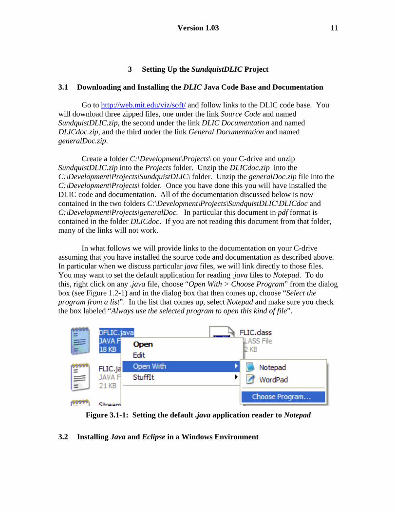
and open the fallingRing.ms MAXScript file. That script will open in an editor window as shown in Figure 6.1-4.

Figure 6.1-4 : The Editor Window for MAX script files.

Using Tools chose Evaluate All. This will run the script. The script creates a torus representing the falling ring, a cylinder representing the magnet, and a screen on which we will “project” the DLICs produced above. The script also computes the motion of the ring for the parameters we used in creating our DLICs above in Section 4.2. It then animates the motion of the ring, producing a 100 frame 3ds max sequence that frame for frame corresponds exactly to our DLIC scenario above. 6.2 Projecting the DLIC on the Screen in the 3ds max Scene To project the DLIC sequence onto the screen, first bring up the Materials Editor

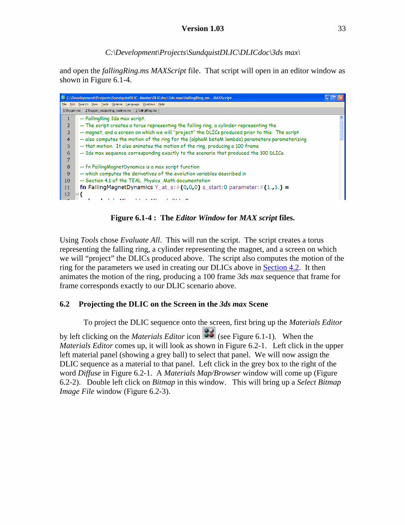
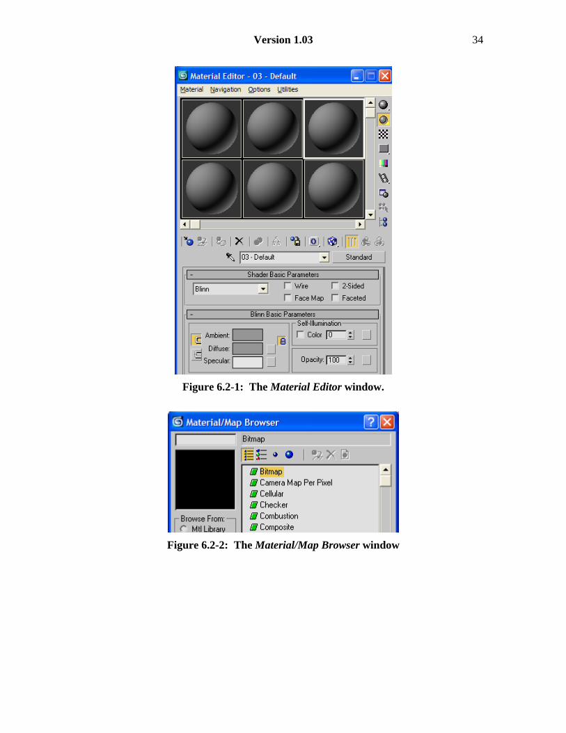
by left clicking on the Materials Editor icon (see Figure 6.1-1). When the Materials Editor comes up, it will look as shown in Figure 6.2-1. Left click in the upper left material panel (showing a grey ball) to select that panel. We will now assign the DLIC sequence as a material to that panel. Left click in the grey box to the right of the word Diffuse in Figure 6.2-1. A Materials Map/Browser window will come up (Figure 6.2-2). Double left click on Bitmap in this window. This will bring up a Select Bitmap Image File window (Figure 6.2-3).

Version 1.03 34

Figure 6.2-1: The Material Editor window.

Figure 6.2-2: The Material/Map Browser window

Version 1.03 35

Figure 6.2-3: The Select Bitmap Image File window

Navigate to the folder

C:\DLICs\fallingRingSM Check the box to the left of Sequence at the bottom of the window in Figure 6.2-3, and left click to select the first image file frsm0000.tif. If you cannot see that file, make sure your “Files of type” box is set either to “All formats” or “TIF Image File (*.tif)”. Then left click on Open. Your Materials Editor window should now look like Figure 6.2-4.

Figure 6.2-4: The Material Editor Icons after assigning the DLIC files

Version 1.03 36

Select the Screen object in 3ds max (left click on the Select by Name box and in the window that comes up select Screen and left click on Select at the bottom of

that window). Then left click on the third icon from the left in the Material Editor window shown in Figure 6.2-4. This assigns the material consisting of the DLIC sequence of images to the Screen. To make the images visible in a 3ds max Viewport,

left-click on the ninth icon from the left in the Material Editor window , and make sure you have chosen Smooth and Highlights for your Viewport window view. You should now see something resembling Figure 4.2-1 in your Front Viewport. When rendered, this scene will produce a 100 frame movie (about 3 seconds long at 30 frames per sec) like the ones shown here (this link opens the folder

C:\Development\Projects\SundquistDLIC\DLICdoc\3ds max\)

We also include in this folder the 3ds max .max file which contains all of the above objects and animations.

7 References

8 Belcher J. W. and S. Olbert, Field Line Motion in Classical Electromagnetism, American

Journal of Physics 71 (3), 220-228, (2003) 9 Belcher, J. and C. Koleci, Using Animated Textures to Visualize Electromagnetic Fields

and Energy Flow, To be submitted to the American Journal of Physics, 2007. 4 Cabral, B. and C. Leedom. Imaging Vector Fields Using Line Integral Convolution. Proc.

SIGGRAPH 1993, pp. 263-270, 1993 4 Liu, Y. and J. Belcher, Magnetic Flux Diffusion and Expulsion with Thin Conducting

Sheets, Submitted to the American Journal of Physics 2007 27 Stalling, D. and H.-C. Hege. Fast and Resolution Independent Line Integral Convolution.

Proc. SIGGRAPH 1995, pp. 249-256, 1995. 8 Sundquist, A, Dynamic line integral convolution for visualizing streamline evolution,

IEEE Transactions on Visualization and Computer Graphics, 9, 273-282, 2003. 4 Sundquist,A., Dynamic Line Integral Convolution for Visualizing Electromagnetic

Phenomena, MIT Master’s Thesis in Engineering in Electrical Engineering and Computer Science and Senior Thesis in Physics, 2001. 4

Version 1.03 37

8 Index

3

3ds max .....................................................................31 3ds max scripting language .......................................31

A

animation class..........................................................15

B

BaseExperiment ........................................................17 BaseObject ................................................................17 blend .........................................................................26 brighten.....................................................................29

C

Cabral and Leedom.....................................................5 change the origin.......................................................15 ChargeInFieldExperiment ........................................30 ChargeMovingAgainstConstantFieldAnimation .......30 CirculatingFlowExperiment......................................22 CirculationFlowAnimation .......................................22 Color Coding ............................................................26 conducting ring ...........................................................8

D

data input ..................................................................24 DataInputAnimation .................................................24 DataInputExperiment................................................24 DataInputObject .......................................................24 default hue for electric fields ....................................20 default hue for magnetic fields..................................23 directory tree.............................................................12 DLIC...........................................................................9 DLIC code base ........................................................11 DLICdoc.zip..............................................................11 downloading Eclipse .................................................12 drift ...........................................................................10

E

eclipse .......................................................................12 electric dipole radiation.............................................21 ElectricOscillatingDipole .........................................22 electromagnetic objects.............................................15 elliptic integrals.........................................................14 EMCollection ............................................................17

EMVec2Field ........................................................... 17 Evaluate All.............................................................. 33 experiment class ....................................................... 15

F

FallingRingAnimation .............................................. 18 FallingRingExperiment ............................................ 18 Fast Line Integral Convolution................................... 9 FieldMotionType ...................................................... 17 FLIC........................................................................... 9 fluid flow.................................................................. 22 Fpower ..................................................................... 23

G

getFlowSpeed ........................................................... 23 getHue ...................................................................... 30 guiding center motion............................................... 10

H

HeliosphereFlowAnimation...................................... 24 HeliosphereFlowExperiment.................................... 24 hints for using Eclipse .............................................. 12 HSV color model...................................................... 27 Hue .......................................................................... 27

I

IDE........................................................................... 12 ImageIO ................................................................... 14 Integrated Development Environment...................... 12 integration schemes .................................................. 14 inter-frame coherence............................................... 10

J

Java SDK.................................................................. 12 javadocs ................................................................... 13

L

line integral convolution............................................. 8 links to the documentation ....................................... 11 Liu and Belcher ........................................................ 29

Version 1.03 38

M

magnetic dipole...........................................................8 material .....................................................................31 Materials Editor........................................................33 Materials Map/Browser ............................................33 memory.....................................................................25 Motion.......................................................................19 motional electric field .........................................17, 21 movie ........................................................................18 MovingPointCharge..................................................19

O

origin of the DLIC ......................................................6 OscillatingDipoleExperiment....................................22 OutputWindow ..........................................................14

P

periodic .....................................................................26 PointCharge..............................................................19

R

render one image.......................................................30 renderer methods......................................................26 rendering parameters.................................................15 RepulsionTwoChargesAnimation..............................19 Run............................................................................25

S

Saturation ............................................................... 27 SinusoidalDipoleRadiationAnimation ...................... 22 Streamline ................................................................ 14 SundquistDLIC.zip ................................................... 11

T

TeachSpinAnimation ................................................ 21 TeachSpinExperiment............................................... 21 TEAL_Physics_Math documentation ....................... 10 texture pattern ............................................................ 6 TwoChargesExperiment ........................................... 19

V

Value........................................................................ 27 variation in field strength ......................................... 29 vector field F(x,t) ....................................................... 9 velocity field ............................................................ 10 velocity field D..................................................... 9, 20 velocity vector field.................................................... 9

Z

zeroes ......................................................................... 8