Dynamic game difficulty balancing in real time using Evolutionary FuzzyCognitive Maps with automatic calibration

Lizeth Joseline Fuentes Perez∗, Luciano Arnaldo Romero Calla†,Anselmo Antunes Montenegro‡, Luis Valente§, Esteban Walter Gonzalez Clua¶∗†‡§¶ Institute of Computing - Federal Fluminense University, Niteroi - RJ

{∗lfuentes, †lromero, ‡anselmo, §lvanlente, ¶esteban}@ic.uff.br

Abstract—Fuzzy Cognitive Maps (FCM) is a paradigm used torepresent knowledge in a simple and concise way, expressingthe grade of relation that exists between concepts and causalrelationships. Due to its flexibility, FCM has been successfullyapplied in numerous applications in diverse research fields,such as, robotics, medical diagnosis, decision problems ininformation technology, games, and so forth. However, onecritical drawback is the determination of the weights in therepresentation graph, which is generally done by an expert.The present paper proposes a semi-automated method forcalibrating the weights in a solution for the problem of dynamicgame difficulty balancing (DGB) using Evolutionary FuzzyCognitive Maps (E-FCM). The proposed algorithm adjuststhe weights in real time, ensuring an equilibrium between thevalues generated according to the expert’s contribution (basedon a static analysis) and the changes produced in the values ofthe concepts by the calibration process during the simulation(a dynamic analysis).

Keywords-Automatic Calibration of Weights, Real-time Strat-egy, Dynamic Game Difficulty Balancing, Evolutionary FuzzyCognitive Maps

I. INTRODUCTION

Along the years, the survival of humanity has been chal-lenged by many factors including, economical, socio-political, ecological and others. Because of that, we ashumans have developed a logic reasoning as a part of acritical thinking that takes part in decision-making processes,which is able to analyze several factors and the relationsamong them.

Due to the increasing complexity of the problems, takingthe right decisions can be, in most of the cases, difficult andtime-consuming. However, with the technology advances wehave been creating algorithms to simulate our reasoningprocess, which currently are still not perfect but can helpus to understand and better control the high complexityassociated to usual decision problems.

One example of these algorithms is the Fuzzy CognitiveMaps (FCM), proposed by Kosko [1], which is considereda hybrid methodology because combines characteristics ofArtificial Neuronal Networks (ANN) and Fuzzy Logic [2].FCM is a powerful tool to simulate complex systems,representing them in a graph, composed of concepts and

causal relations, which describe the way the concepts arerelated to each other. The causal relationships also measurethe degree to which one concept affects another, which isrepresented by a weight.

Even though FCM have been applied in numerous researchfields and applications, such as: Robotics, for example fornavigation of robots [3], medical decision making [4], forexample, radiotherapy [5], risk management [6], bankingmanagement [7], information technology [8], computer vi-sion [9], controllers and supervisory agents of complexsystems [10] and so forth; however, in the literature, thereare few works devoted to the solution of one critical issue:the determination of the weights of the causal relationships,which is generally done by an expert.

The algorithms that focus on solving the fully automaticcalibration, as far as we are concerned, can be categorizedinto three classes: the Hebbian learning based methods [11],Neuronal Networks Based methods [12], and the Geneticalgorithms based methods [13]; we refer the interested readerto the work in [14], where some of these methods arecompared.

The calibration of the weights in the FCM design stepcan be performed in two ways: using expert-based methodsand performing fully automatic calibration. These two ap-proaches have differences and characteristics that are brieflydelineated below:

• In expert-based methods, the calibration depends on theexperts’ subjective judgment, which can introduce someerrors in the simulation. Usually, the calibration is doneby computing an average of the experts’ judgmentsusing a deductive reasoning. In this approach, as itis based on the expert’s own beliefs, it is easy todevise a set of weights that is coherent with the staticbehavior expected for the system. On the other hand,it is not possible to guarantee that the system willbehave as expected during the simulation (the dynamicbehavior). This usually happens when the complexityof the problem grows. As the number of conceptsand causal relationships increase, the experts cannotconsider the problem as a whole. They are obliged to

38 SBC Journal on Interactive Systems, volume 7, number 1, 2016

ISSN: 2236-3297

Figure 1: TimeOver Game

group the concepts and causal relationships into partsmaking difficult any global analysis and prediction ofhow the system will evolve from the initial static setup.

• The fully automatic calibration algorithms require as aninput, a priori knowledge of the system, which can beobtained from different sources, for example using datamining. From this initial input, an inductive learningprocess extracts a set of rules which are used to generatethe weights in the FCM. Such methods are prone toproduce stable dynamical behavior.

In a few words, expert-based approaches are good for coher-ent static weight definition and fully automatic algorithmsare adequate for achieving a stable dynamic behavior. Themain contribution of this work is a new method that hasboth good properties. It is based on a dynamic automaticcalibration which combines expert knowledge with a real-time automatic weight adjustment.

We specifically applied our method to the solution of thedynamic game difficulty balancing problem that uses Evo-lutionary Fuzzy Cognitive Maps (E-FCM).

Evolutionary Fuzzy Cognitive Map (E-FCM) extends FCMproposed by [15], [16], where each state is evolving ac-cording to non-deterministic external causalities. Similar tothe FCM, Evolutionary Fuzzy Cognitive Maps have beenalso applied to a variety of scientific areas, such as politicaldecision making [17], interactive storytelling for the creationof virtual worlds [16], medical diagnosis [18], [19], compu-tation pragmatics [20] and so forth.

In [21], the authors proposed a method to change thedifficulty levels dynamically and in real-time, which isbased on player interaction information, context variables,and Evolutionary Fuzzy Cognitive Maps. Player interactionsinvolve actions where the player interacts directly with thegame logic, for example, eating, jumping or collecting items.

The method proposed in [21], is different from othersproposed in literature [22], [23], [24], because it presents

three important advantages: independence, adaptability, andscalability.

Independence, because the method is able to adjust thedifficulty levels independently of explicit player feedback(e.g., surveys, reports, and related alternatives) inferring thenecessary information directly from player actions in thegame.

Adaptability, because it is possible to apply the method toany game, as E-FCM are flexible.

Scalability because, as the number of context variables andcausal relationships increase, it is possible to consider morefactors to evaluate player-related aspects, which may lead tobetter game experience and player engagement.

This paper is organized as follows. Section II presentsan overview of Evolutionary Fuzzy Cognitive Maps (E-FCM). Section III describes the application of E-FCM forDynamic Game Difficulty Balancing. Section IV describesthe algorithm proposed for weights calibration in real-time.Section V presents experimental results and Section VIpresents conclusions and future works.

II. EVOLUTIONARY FUZZY COGNITIVE MAPS

In this section, we present the components of the E-FCMmodel and how simulations in real-time can be performedusing an updating step. The design of an E-FCM is basicallythe design of a FCM adding the evolving time.

A. E-FCM Design

An E-FCM is constructed with two main components:concepts and causal relationships.

• Concepts C = (S,∆S,T,Ps), which represents importantfactors and characteristics of the real-time system. Eachconcept c ∈C is expressed as a tuple:

SBC Journal on Interactive Systems, volume 7, number 1, 2016 39

ISSN: 2236-3297

c = (s,∆s,et, ps) (1)

where, s ∈ S denotes the value or level of the concept,et ∈ T is the evolving time for the concept and ps isthe probability of self-mutation. ∆s ∈ ∆S is the statevalue change for the concept, which will be updated inreal-time simulations.The evolving time et is important in a real-time systembecause it helps to control the change of the conceptvalue s, at a given instant of time t.For example: Given two concepts in vital functions ofthe human being system: breathe and eat, it is requiredthat the value of breathe to be updated every fiveseconds, whereas the value of eat can be updated everysix hours.Different concepts might have different evolving times.Let C be a set with n concept variables. The set of itsevolving times can be represented in vectorial form as

T =

et1et2...

eti...

etn

(2)

The concepts in the system have their states updated intheir respective evolving times. Besides, each conceptalternates its internal state randomly in real time. Thus,to each concept we associate a very small mutationprobability ps. If the probability is high, the systemcan become very unstable.

• Causal relationship (ri j), which represents the strengthand probability of the causal effect from one conceptci to another concept c j. It is defined as a tuple:

ri j = (wi j,s, pmi j) (3)

where wi j is the weight of the causal relationship anddenotes the degree of influence of the concept ci tothe concept c j. The weights are fuzzy values; they cannormally be in the range of [−1,1] or [0,1].The relationships between the concepts can be director inverse. This is expressed in the variable s, whichcan be positive or negative, describing respectively thedirect or inverse relationships.In the E-FCM model, concepts can be affected bycausal relationships with probability pm.Figure 2 illustrates how an E-FCM model describescausality. In the example, the concept c1 affects theconcept c2 via a causal relation c1 → c2, where c1 isthe causal variable and c2 is the effect variable.

u1

u2

C3

PI

C2

C1

C4

Cnum

E-FCM

Figure 2: E-FCM modified to include ui relationships,related to player interactions (PI). Ci represents contextvariables and dotted arrows represent the causal relation-ships.

In our examples, in each causal relationship, we considerthe probabilities pm = 1, and the signs are implicitly de-fined in the weights wi j ∈ [−1,1]. Thus, the fuzzy causalrelationships for a system with n variables can be directlyrepresented as a n×n weight matrix W :

W =

w11 w12 · · · w1nw21 w22 · · · w2n

...... · · ·

...wi1 wi j · · · win

...... · · ·

...wn1 wn2 · · · wnn

(4)

B. Updating step for Simulations in Real Time

E-FCM works updating in each cycle all the context vari-ables, states S, whenever a evolving time et of a concept cmatches the current time value t. This update is a funda-mental step in the theory of E-FCM and is called a runningcycle [2].

The state value si of a concept is updated at time step t +1from the previous time step t by computing its state changeaccording to equation (5):

∆st+1i = k1

n

∑j=0, j 6=i

h(pmi j−λ )∆stjwi j + k2∆st

i (5)

where h is the Heaviside step function:

h(x) =

{0, n < 01, n≥ 0

40 SBC Journal on Interactive Systems, volume 7, number 1, 2016

ISSN: 2236-3297

and λ is a probability threshold between 0 and 1. As wedefined the probabilities pm = 1, equation (5) can be writtenin a simplified version:

∆st+1i = k1

n

∑j=0, j 6=i

∆stjwi j + k2∆st

i (6)

st+1i = f

(st

i +∆st+1i)

(7)

where f is the activation function used to regulate the statevalue. It is important to adjust the concepts values in a givenrange. Some usual f functions are:

• Bipolar, for binary values 0 or 1.• Logistics, for values in the range [0,1]:

f (x) =1

1+ e−λx (8)

where λ � 0.• Hyperbolic, for values in the range [−1,1]:

f (x) = tanh(x). (9)

The state value of the concept ci at time t is representedas si. The state value change of the concept ci at time t is∆st . The evolving time et is not included in this formulabecause it is used to verify in which running cycle si mustbe updated. Different concepts may have different evolvingtimes. The k1 and k2 values are constants; k2 represents theproportional contribution of the other concepts which affectsto ci and k1 represents the influence of the previous valuesi.

III. USING E-FCM FOR DYNAMIC GAME DIFFICUTLYBALANCING

In this section, we will explain briefly, the design of theE-FCM used to solve the DGB problem.

In [21], the authors introduced the player interactions asinputs that change the E-FCM values in real-time.

Note that with such introduction the E-FCM is able to simu-late different behaviors along the gameplay. For example, theE-FCM provides to the player more items when his staminais low. Conversely, when his stamina is high, the E-FCMincreases the number and difficulty of the obstacles.

In this work, we use the Time Over game presented in [21],as a study case. This is a runner type game where the playeris a boy who is escaping from a twister. In the game, he mustavoid the obstacles and also collect some items such as foodand water, which are provided to him to recover his energy.Figure 1 illustrates some screenshots of the TimeOver game.

One interesting feature of Time Over game is that theplayer’s energy is not infinite. Hence, a tiredness factor is

considered, which will affect the player’s energy and also hisspeed. Thus, the player is forced to collect items constantlyto survive.

According to this game description, the game designerconsiders the following concepts as context variables:

1) Stamina: represents the player’s energy, which in-creases as the player collects more items in the game.

2) Speed: represents the player’s speed, which relates tostamina. Speed decreases over time to simulate theplayer character’s tiredness.

3) Obstacle type: there are three types of obstacles: easy,default, and hard. These types represent how difficultthe obstacles are.

4) Obstacle period: represents the period (time interval)that the game uses to insert obstacles in the gamescene.

5) Item type: there are two types of collectible items inthe game: water bottles and seeds. Both items increaseplayer stamina, but water bottles provide more staminathan seeds.

6) Item period: represents the period (time interval) thatthe game uses to insert collectible items in the gamescene.

In practice, players have different skill levels and may regardusual predetermined difficult levels as too easy or too hard,becoming frustrated or bored. For that reason, the gamedesigner sets rules to keep the player on playing the game.Some examples of rules for this case are:

• If the player’s energy increases, the speed also in-creases.

• If the player’s speed is high, the number of food andwater is reduced and the difficulty of the obstacles isincreased.

Based on this rules, the game designer creates the causalrelationships between concepts and decides whether therelation is direct or inverse. In this stage, it is importantto define the degree of the causalities (the weights). Thedefinition of the weights is a critical step because it controlsthe gameplay experience. Weights with high values alongthe gameplay can produce instability in the E-FCM becausethe changes are more violent. Weights with very low valuescan produce low interactivity along the gameplay, and it isnot desired in real-time simulations.

According to [21], the new function that updates the con-cepts values, including the player interactions (ui), is asfollows:

∆st+tii = f

(k1

n

∑j=0

∆stjwi j + k2(∆st

i +ui)

)(10)

SBC Journal on Interactive Systems, volume 7, number 1, 2016 41

ISSN: 2236-3297

The player interactions ui drastically alter the behavior of theE-FCM, so dynamically changes the game difficulty levelsin real-time. However, this changes could produce abruptchanges in the game experience. Thus, it is necessary toachieve an equilibrium between the game designer expecta-tion’s, who knows the game logic, and the behavior of theE-FCM along the gameplay. The present paper proposes analgorithm to adjust the weights, using an initial configurationgiven by the game designer and controlling the ratio ofchanges in the E-FCM to improve the gameplay experience.

IV. CALIBRATING E-FCM WEIGHTS

So far, we detailed how E-FCM works, however, the gameexperience does not only depends on the correct work ofthe logic rules for DGB. Along the gameplay, it is alsoimportant that the game level changes are not abrupt becauseit generates instability in the game experience.

In the gameplay for example, if stamina decreases quickly,the other inverse concepts to stamina will increase so fast,that a lot of items will be generated in a short time.

In every instant of time, a running cycle is executed. Algo-rithm 1 summarizes the process of updating the concepts’values in a running cycle of E-FCM.

Algorithm 1 E-FCM running cycle in real-time

Require: C = (S,T ): conceptsRequire: W : weight matrixRequire: t: current timeRequire: ∆St : states value change at time t

1 ∆St+1⇐ ∆St

2 for all ci ∈C do3 if t mod ti = 0 then

4 ∆st+1i ⇐ f

(k1

n

∑j=1,i6= j

∆stjwi j + k2(∆St

i +ui)

)

5 st+1i ⇐ st

i +∆st+1i

6 end if7 end for

When the simulation is finished, the E-FCM producesfunctions (time series) for each concept, influenced by theplayer interactions. In general applications, the conceptsof E-FCM tend to converge, according to the logic of E-FCM design. However, since the player interactions wereintroduced, the E-FCM concepts values are always changingalong the gameplay. Because of that, it is necessary tocontrol the changes in the values of the concepts avoidingabrupt changes along the simulations.

To cope with this issue, since it is impossible to predict thebehavior of the functions as they strongly depend on playerinteractions, we consider two fundamental E-FCM elementsthat are known in each running cycle:

The weights wi j and the state value change ∆si,∆s j, whichindicates how the functions are changing at an instant oftime.

In order to define a way to update the weights, so thatthe functions evolve in a smooth way, keeping the coher-ence with the causal relationships, we analyse the fourbasic combination of function behaviors and associatedstate changes. In each configuration we analyse the relationbetween function growth or decrease and the state changevalues and how the weights can be modified to control thefunction behavior.

• Direct and increasing relation wi, j > 0 and ∆si >0,∆s j > 0, when both functions are increasing. In thiscase, the weight is reduced proportionally to the conceptchanges, to moderate the independence degree betweenthe functions associated to the concepts.

• Direct and decreasing relation wi, j > 0 and ∆si <0,∆s j < 0, when both functions are decreasing. In thiscase, the weight is also reduced proportionally to theconcept changes, to reduce the independence degreebetween the functions of the concepts.

• Indirect and increasing-decreasing relation wi, j < 0and ∆si > 0,∆s j < 0, when the function generated bythe causal concept ci is increasing and the functiongenerated by the effect concept c j is decreasing. In thiscase, the two functions are moving away from eachother, depending on the weight. Since ci affects to c j,it is necessary to reduce the repulsion force, increasingthe weight in a factor proportional to the changes ofthe functions. The increase in the weight makes thecausal concept have more influence in the effect conceptmaking them have a closer behavior.

• Indirect and decreasing-increasing relation wi, j < 0and ∆si < 0,∆s j > 0, when the function generated by thecausal concept ci is decreasing and the function gener-ated by the effect concept c j is increasing. In this case,the two functions are approaching each other. Since ciaffects to c j, it is necessary reduce the attraction forcealso the weight is increased in a proportional factorto the changes of the functions. As in the previouscase, the increase in the weight has the same effect.Both variables will have greater correlation, as thecausal variable will have more impact on the effectvariable, diminishing the difference in the behavior ofthe functions, caused by the sign difference in the statechanges ∆si and ∆s j.

From the analysis, we update the weights is real-timeaccording to equation (11):

wi j = f (wi j(1−∆Sti∆St

j)) (11)

42 SBC Journal on Interactive Systems, volume 7, number 1, 2016

ISSN: 2236-3297

where f is the regularization function which guarantees thatthe weight values are always in range [−1,1].

Finally, we developed a new algorithm, seen in Algorithm2, wherein each running cycle the weights are adjusted,considering the changes of the concept levels. In the algo-rithm ∆st

i∆stj, represents the strength of the weight change,

and if this is positive or negative. The adjustment is justproportional to the old weight according to wi j⇐ f (wi j(1−∆st

i∆stj)).

Algorithm 2 Update E-FCM real time with calibration

Require: C = (S,T ): conceptsRequire: W : weight matrixRequire: t: current timeRequire: ∆St : states value change at time t

1 ∆St+1⇐ ∆St

2 for all ci ∈C do3 if t mod ti = 0 then4 wi j⇐ f (wi j(1−∆st

i∆stj))

5 ∆st+1i ⇐ f

(k1

n

∑j=1,i6= j

∆stjwi j + k2(∆st

i +ui)

)

6 st+1i ⇐ st

i +∆st+1i

7 end if8 end for

Algorithm 2 summarizes the process of automatic calibrationof weights in real-time.

V. EXPERIMENTS AND RESULTS

In order to experimentally validate our algorithm, we createdthe Social Drug E-FCM and also redesigned the E-FCM forthe Time Over game.

A. Social Drug E-FCM

“Social Drug” E-FCM basically simulates the human emo-tions and its emotional states when a person experimentssocial approval (flattery) or social rejection (understate).

Figure 3, illustrates the E-FCM model for “Social Drug”,where the context variables are:

• c1: Animus.• c2: Depression.• c3: Sadness.• c4: Courage.• c5: Health.• c6: Happiness.

The player interactions u1 and u2, represent social approvaland social rejection respectively.

C1

C2

C3

C5

C6

C4

+

_

u1

u2

_

+

+

_

_

_

+

_

+

_

_

++

+

Figure 3: The E-FCM model for Social Drug.

0Animuss: 0.6

Δs: 0.001t: 1

2Sad

s: 0.5Δs: 0.001

t: 2

-0.5

3Encouraged

s: 0.55Δs: 0.001

t: 2

0.3

5Happys: 0.6

Δs: 0.001t: 3

0.4

1Depression

s: 0.5Δs: 0.001

t: 5

-0.6

-0.2

0.8

-0.75-0.1

4Healthys: 0.7

Δs: 0.001t: 5

0.4

0.4

-0.25

-0.3

0.3 0.6

Figure 4: The E-FCM model for Social Drug.

The evolving time vector is T = (1 1 2 2 5 3) andthe initial values for the context variables are

SBC Journal on Interactive Systems, volume 7, number 1, 2016 43

ISSN: 2236-3297

0Animus

s: 0Δs: 0.059

t: 1

2Sads: 1

Δs: 0.013t: 2

-0.17

3Encouraged

s: 0Δs: -0.013

t: 2

0.087

5Happy

s: 0.0061Δs: 0.0061

t: 3

0.46

1Depression

s: 0.98Δs: 0.01

t: 5

-0.5

-0.12

0.69

-0.46-0.061

4Healthys: 0.5

Δs: 0.0024t: 5

0.32

0.37

-0.22

-0.24

0.23 0.57

Figure 5: The E-FCM model for Social Drug.

S0 = (0.6 0.5 0.5 0.55 0.7 0.6)

.

Figures 6, 7, illustrates the simulations of E-FCM SocialDrug, where the interactions “Social Approval” and “SocialRejection” were simulated altering both values, emphasizingthe factor “Social Rejection”. Because of this, along thesimulation the concept ”Animus” is decreasing in bothcalibrated and non-calibrated simulations.

The main difference between figures 6 and 7 is the behaviorof the concept (state values) along the time. In Figure 6,we can observe that the concept values of Animus, Courage,Health and Happiness are decreasing faster than the conceptvalues with calibrated weights. Moreover, the behavior atinitial times is quite similar, which is an expected behaviorbecause the calibration process is done along the simulationsin real-time and also depends on the player interactions. Theweights adjustment would be impossible to do in the game

design stage because is impossible to predict how the playerwill interact with the E-FCM along the simulations.

Therefore, for different gameplays, the algorithm will pro-duce different weight matrices. In the case of the SocialDrug model, we applied the same interactions in bothsimulations, the calibrated and non-calibrated, in order tobetter appreciate the effect of the calibration algorithm alongthe simulations.

Figure 6 shows the E-FCM behavior along the first 100 timeinstances, setting as initial configuration the E-FCM modelillustrated in Figure 4; the convergence is reached close tot = 100 and the final configuration is shown in Figure 5.

The concepts’ values converge to 0 and 1, keeping the logicin the causal relations, but it should be noted that the Healthconcept converges slower than the other concepts.

Conversely, in Figure 7, which shows the simulation withweights calibration, not all concept’s values converge to 0or 1 in time t = 100. The value of Health concept in thistime is 0.5, and its curve did not drop to 0. It should benoted that the curve for the Happiness concept converges to0, but it takes longer than in the non-calibrate graph whosevalue is already 0 in t = 60.

In the same way, Depression curve increases much slower,in t = 100 it still has not reached the value of 1.

Figure 7 shows the simulation of the E-FCM with calibratedweights. It is possible to see that the curves of the conceptschange slower than those obtained in the simulation with thenon calibrated E-FCM. This real-time calibration guaranteesthat changes in game difficulty are not abrupt, differentlyfrom those presented in [21].

Table I, shows the probabilistic weight output matrix Wof the causal relationship for the Social Drug experiment,obtained after the weights were calibrated via the proposedalgorithm.

Table I: Probabilistic weight matrix W of the causal rela-tionship for Social Drugs

wi j c1 c2 c3 c4 c5 c6c1 0 0 -0.77 0.72 0 0.72c2 0 0 0 0 0 0.9899c3 -0.55 0.72 0 -0.88 0 0c4 0 0 -0.33 0 0 0c5 0.54 0 0 0 0 0c6 0.54 -0.33 -0.55 0.72 0.81 0

B. Time Over E-FCM

We also validate our model in a game, where the interactionsare different from those in the Social Drug case. We runthe E-FCM model with different player interactions, but

44 SBC Journal on Interactive Systems, volume 7, number 1, 2016

ISSN: 2236-3297

-0.1

0

0.1

0.2

0.3

0.4

0.5

0.6

0.7

0.8

0.9

1

1.1

0 2 4 6 8 1

0 1

2 1

4 1

6 1

8 2

0 2

2 2

4 2

6 2

8 3

0 3

2 3

4 3

6 3

8 4

0 4

2 4

4 4

6 4

8 5

0 5

2 5

4 5

6 5

8 6

0 6

2 6

4 6

6 6

8 7

0 7

2 7

4 7

6 7

8 8

0 8

2 8

4 8

6 8

8 9

0 9

2 9

4 9

6 9

8 1

00

valu

e

time

animusdepression

sadencouraged

healthyhappy

Figure 6: E-FCM simulation without calibrated weights in the Social Drug model

-0.1

0

0.1

0.2

0.3

0.4

0.5

0.6

0.7

0.8

0.9

1

1.1

0 2 4 6 8 1

0 1

2 1

4 1

6 1

8 2

0 2

2 2

4 2

6 2

8 3

0 3

2 3

4 3

6 3

8 4

0 4

2 4

4 4

6 4

8 5

0 5

2 5

4 5

6 5

8 6

0 6

2 6

4 6

6 6

8 7

0 7

2 7

4 7

6 7

8 8

0 8

2 8

4 8

6 8

8 9

0 9

2 9

4 9

6 9

8 1

00

valu

e

time

animusdepression

sadencouraged

healthyhappy

Figure 7: E-FCM simulation with calibrated weights in the Social Drug model

with the same player. Figure 8 shows the E-FCM modelfor TimeOver game.

Each context variable describes is a fuzzy value, normalizedto the range [0,1]. The mean of each variable value dependson specific game designs. For simplicity, we defined obstacletype as a mapping of the actual value of obstacle type toconceptual “easy”, “default”, and “hard” difficulty obstaclelevels. The “easy” difficulty level maps to the range of[0,0.33], the “default” difficulty level maps to [0.34,0.66]and the “hard” level maps to the range of [0.66,1]. The

Item type is a mapping of the actual value of item typeto conceptual “water” and “seeds”. The water item appearswhen the corresponding value belongs to the range [0,0.5].The seed item appears when the corresponding values arein the range [0.6,1]. We associate each context variable tothe following concepts:

• c1: Stamina.• c2: Speed.• c3: Obstacle type.• c4: Obstacle period.

SBC Journal on Interactive Systems, volume 7, number 1, 2016 45

ISSN: 2236-3297

C1 C2 C3

C5 C6 C4

+

_+

+

_+

+

_

u1

u2

Figure 8: The E-FCM model for TimeOver game.

0stamina

s: 1Δs: 0.01

t: 1

1velocity

s: 1Δs: 0.001

t: 4

1

4items_type

s: 0.2Δs: 0.1

t: 1

-0.8

5items_freq

s: 0.9Δs: 0.1

t: 1

0.1

2obstacle_type

s: 0.8Δs: 0.1

t: 1

1

3obstacle_freq

s: 0.1Δs: 0.1

t: 1

-0.8 0.9

Figure 9: The initial E-FCM configuration for TimeOvergame.

• c5: Item type.• c6: Item period.

Figure 8 illustrates the final TimeOver’s E-FCM model,where ci, i ∈ [1,6] represents each context variable andsigned arrows represent causal relationships between contextvariables. A positive sign (+), means positive causal rela-tionship and negative sign (−) means negative relationship.Table II illustrates the probabilistic weight matrix W ofcausal relationships, which are determined either from anexpert knowledge or learned from a knowledge base. In thispaper we redesigned some of these values; as the modeldesigned for this game is simple, the weights were provided

0staminas: 0.98

Δs: -0.00022t: 1

1velocitys: 0.65

Δs: -0.0022t: 4

1

4items_type

s: 0.29Δs: 0.0018

t: 1

-0.8

5items_freq

s: 0.23Δs: -0.0022

t: 1

0.1

2obstacle_type

s: 0.25Δs: -0.0022

t: 1

1

3obstacle_freq

s: 0.8Δs: 0.0018

t: 1

-0.8 0.9

Figure 10: The E-FCM model result without calibration forTimeOver game.

0staminas: 0.76

Δs: -0.00022t: 1

1velocitys: 0.8

Δs: -0.0022t: 4

1

4items_type

s: 0.64Δs: 0.0022

t: 1

-1

5items_freq

s: 0.17Δs: -0.0006

t: 1

0.099

2obstacle_type

s: 0.37Δs: -0.00043

t: 1

0.19

3obstacle_freq

s: 0.62Δs: 0.0022

t: 1

-1 0.17

Figure 11: The E-FCM model resut with calibration forTimeOver game.

by the game designer. The matrix Pm is a one’s matrixbecause we consider that the probability of a concept ciaffecting another concept c j is equal to one.

The activation function selected for the experiments was the

46 SBC Journal on Interactive Systems, volume 7, number 1, 2016

ISSN: 2236-3297

-0.1

0

0.1

0.2

0.3

0.4

0.5

0.6

0.7

0.8

0.9

1

1.1

0 5

0 1

00

150

200

250

300

350

400

450

500

550

600

650

700

750

800

850

900

950

1000

1050

1100

1150

1200

1250

1300

1350

1400

1450

1500

1550

1600

1650

1700

1750

1800

1850

1900

1950

2000

2050

2100

2150

2200

2250

2300

2350

2400

2450

2500

2550

2600

2650

2700

2750

2800

2850

valu

e

time

staminaspeed

obstacle typeobstacle period

items typeitems period

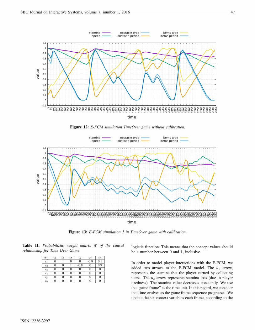
Figure 12: E-FCM simulation TimeOver game without calibration.

-0.1

0

0.1

0.2

0.3

0.4

0.5

0.6

0.7

0.8

0.9

1

1.1

0 5

0 1

00

150

200

250

300

350

400

450

500

550

600

650

700

750

800

850

900

950

1000

1050

1100

1150

1200

1250

1300

1350

1400

1450

1500

1550

1600

1650

1700

1750

1800

1850

1900

1950

2000

2050

2100

2150

2200

2250

2300

2350

2400

2450

2500

2550

2600

2650

2700

2750

2800

2850

2900

2950

3000

3050

3100

3150

3200

3250

3300

3350

3400

3450

3500

3550

3600

3650

3700

3750

3800

3850

3900

3950

4000

4050

valu

e

time

staminaspeed

obstacle typeobstacle period

items typeitems period

Figure 13: E-FCM simulation 1 in TimeOver game with calibration.

Table II: Probabilistic weight matrix W of the causalrelationship for Time Over Game

wi j c1 c2 c3 c4 c5 c6c1 0 1 0 0 -0.8 0.1c2 0 0 1 -0.8 0 0.9c3 0 0 0 0 0 0c4 0 0 0 0 0 0c5 0 0 0 0 0 0c6 0 0 0 0 0 0

logistic function. This means that the concept values shouldbe a number between 0 and 1, inclusive.

In order to model player interactions with the E-FCM, weadded two arrows to the E-FCM model. The u1 arrow,represents the stamina that the player earned by collectingitems. The u2 arrow represents stamina loss (due to playertiredness). The stamina value decreases constantly. We usethe “game frame” as the time unit. In this regard, we considerthat time evolves as the game frame sequence progresses. Weupdate the six context variables each frame, according to the

SBC Journal on Interactive Systems, volume 7, number 1, 2016 47

ISSN: 2236-3297

evolving time vector T :

T = (1 4 1 1 1 1)

The values in T denote the time interval in which a variableis updated. For example, a value equal to 1 means that avariable is updated each frame. A value equal to 2 meansthat a variable is updated every two frames, and so on. Herewe modified the speed evolving time value to 4 because weconsider the speed changes in the player must be slower.

The initial values of the six context variables are:

S0 = (0.01 0.001 0.1 0.1 0.1 0.1)

Figure 9, illustrates the initial configuration of E-FCM forTimeOver game. Figures 11 and 13 illustrate the configu-ration results of real-time simulations that we designed andconducted to test the behavior of E-FCM model with non-calibrate and calibrate weights respectively.

Figures 12 and 13 illustrate the context variables in eachgame frame. Given the initial configuration in Figure 9, weexpected that in the simulations, the concept values changeas the player interact along the game. Each figure illustratesthe context variables in each game frame, demonstrating thatall simulations behaved as we expected.

Figures 12 and 13 are different, because the player interac-tions were performed in different ways. However, in bothgameplays, the concept values changes according to the E-FCM model.

One remarkable difference between both gameplays, thecalibrated and the non-calibrated, is the behavior of the func-tions (concepts values in each game frame). In Figure 13,the “obstacle type” and “items period” functions, becomingmore independent of each other along the gameplay.

The functions of the concepts in Figure 13 present lessabrupt changes, for example in frame 300, when the value ofstamina decreases, the values of “speed”, “items period” and“obstacle type” also decreases but the change is smoothercompared with the frame 2515 of the gameplay in Figure12 with non-calibrate weights.

VI. CONCLUSIONS

Considering the results described in Section V, we observedthat our algorithm enhances the gameplay experience, be-cause it is able to regularize the changes produced by theplayer interactions, avoiding abrupt changes and consideringonly the principal elements of the causal relations such as:inverse or direct causal relationships (positive or negativesign) and the degrees of change (∆S).

Therefore, we conclude that our algorithm generates softersimulations in real-time, considering the player interactionsand also presents the following advantages:

Dynamic: The proposed algorithm takes advantageof the dynamic behavior of the E-FCM to generatethe regularization of the functions in real-time.Independence: The method considers mainly theown natural evolution the E-FCM. It does notrequire any external method for smoothing thefunctions.Coherence: The smooth functions will always becoherent with the E-FCM design. In the case ofour method, coherence is automatically obtainedbecause the regularization of the functions reliessolely on the data captured directly from the E-FCM simulation. It would be necessary more ex-periments to verify if other regularization methods,for example, those based on time-series smoothingor moving averages, would lead to convergence andpresent results coherent with the design of the E-FCM. This is something that we achieve withoutintroducing external processes.

An interesting future work is a in depth study of the behaviorof the E-FCM models in real-time, that is, to figure out howto predict its behavior in real-time simulations from the gamedesign. Another interesting work is to do an analysis of thegame experiences using E-FCM and E-FCM with calibrationbecause it is possible to find out other factors that may helpto improve the game experience based on this methodology.

ACKNOWLEDGEMENTS

We thank CAPES, CNPq, FAPERJ and NVIDIA for sup-porting the present research.

REFERENCES

[1] B. Kosko, “Fuzzy cognitive maps,” Int. J. Man-Mach. Stud.,vol. 24, no. 1, pp. 65–75, Jan. 1986. [Online]. Available:http://dx.doi.org/10.1016/S0020-7373(86)80040-2

[2] P. P. Groumpos, Fuzzy Cognitive Maps: Basic Theories andTheir Application to Complex Systems. Berlin, Heidelberg:Springer Berlin Heidelberg, 2010, pp. 1–22. [Online].Available: http://dx.doi.org/10.1007/978-3-642-03220-2 1

[3] D. Lorencik, J. Vascak, and M. Vircikova, Adaptive FuzzyCognitive Maps Using Interactive Evolution: A RobustSolution for Navigation of Robots. Berlin, Heidelberg:Springer Berlin Heidelberg, 2013, pp. 703–711. [Online].Available: http://dx.doi.org/10.1007/978-3-642-37374-9 67

48 SBC Journal on Interactive Systems, volume 7, number 1, 2016

ISSN: 2236-3297

[4] C. D. Stylios, V. C. Georgopoulos, G. A. Malandraki, andS. Chouliara, “Fuzzy cognitive map architectures for medicaldecision support systems,” Applied Soft Computing, vol. 8,no. 3, pp. 1243 – 1251, 2008, forging the Frontiers - - SoftComputing. [Online]. Available: http://www.sciencedirect.com/science/article/pii/S1568494607001226

[5] E. I. Papageorgiou, A Novel Approach on Constructed Dy-namic Fuzzy Cognitive Maps Using Fuzzified Decision Treesand Knowledge-Extraction Techniques. Berlin, Heidelberg:Springer Berlin Heidelberg, 2010, pp. 43–70. [Online].Available: http://dx.doi.org/10.1007/978-3-642-03220-2 3

[6] S. M. Hurtado, Modeling of Operative Risk UsingFuzzy Expert Systems. Berlin, Heidelberg: SpringerBerlin Heidelberg, 2010, pp. 135–159. [Online]. Available:http://dx.doi.org/10.1007/978-3-642-03220-2 6

[7] G. Xirogiannis, M. Glykas, and C. Staikouras,Fuzzy Cognitive Maps in Banking Business ProcessPerformance Measurement. Berlin, Heidelberg: SpringerBerlin Heidelberg, 2010, pp. 161–200. [Online]. Available:http://dx.doi.org/10.1007/978-3-642-03220-2 7

[8] J. L. Salmeron, Fuzzy Cognitive Maps-Based IT ProjectsRisks Scenarios. Berlin, Heidelberg: Springer BerlinHeidelberg, 2010, pp. 201–215. [Online]. Available: http://dx.doi.org/10.1007/978-3-642-03220-2 8

[9] G. Pajares, M. Guijarro, P. J. Herrera, J. J. Ruz,and J. M. de la Cruz, Fuzzy Cognitive Maps Appliedto Computer Vision Tasks. Berlin, Heidelberg: SpringerBerlin Heidelberg, 2010, pp. 259–289. [Online]. Available:http://dx.doi.org/10.1007/978-3-642-03220-2 11

[10] A. Jose, Dynamic Fuzzy Cognitive Maps for the Supervisionof Multiagent Systems. Berlin, Heidelberg: Springer BerlinHeidelberg, 2010, pp. 307–324. [Online]. Available: http://dx.doi.org/10.1007/978-3-642-03220-2 13

[11] E. Papageorgiou, C. Stylios, and P. Groumpos, “Activehebbian learning algorithm to train fuzzy cognitive maps,”International Journal of Approximate Reasoning, vol. 37,no. 3, pp. 219 – 249, 2004. [Online]. Available: http://www.sciencedirect.com/science/article/pii/S0888613X04000349

[12] H. Song, C. Miao, Z. Shen, W. Roel, D. Maja, andC. Francky, “Design of fuzzy cognitive maps usingneural networks for predicting chaotic time series,” NeuralNetworks, vol. 23, no. 10, pp. 1264 – 1275, 2010.[Online]. Available: http://www.sciencedirect.com/science/article/pii/S0893608010001541

[13] E. I. Papageorgiou and P. P. Groumpos, “A new hybridmethod using evolutionary algorithms to train fuzzy cognitivemaps,” Applied Soft Computing, vol. 5, no. 4, pp. 409– 431, 2005. [Online]. Available: http://www.sciencedirect.com/science/article/pii/S1568494604001012

[14] W. Stach, L. Kurgan, and W. Pedrycz, Expert-Based andComputational Methods for Developing Fuzzy CognitiveMaps. Berlin, Heidelberg: Springer Berlin Heidelberg,2010, pp. 23–41. [Online]. Available: http://dx.doi.org/10.1007/978-3-642-03220-2 2

[15] Y. Cai, C. Miao, A.-H. Tan, and Z. Shen, “Context mod-eling with evolutionary fuzzy cognitive map in interactivestorytelling,” in Fuzzy Systems, 2008. FUZZ-IEEE 2008.(IEEE World Congress on Computational Intelligence). IEEEInternational Conference on, June 2008, pp. 2320–2325.

[16] Y. Cai, C. Miao, A.-H. Tan, Z. Shen, and B. Li, “Creatingan immersive game world with evolutionary fuzzy cognitivemaps,” Computer Graphics and Applications, IEEE, vol. 30,no. 2, pp. 58–70, March 2010.

[17] A. S. Andreou, N. H. Mateou, and G. Zombanakis,“Evolutionary fuzzy cognitive maps: A hybrid systemfor crisis management and political decision making,”University Library of Munich, Germany, MPRA Paper, 2003.[Online]. Available: http://EconPapers.repec.org/RePEc:pra:mprapa:51482

[18] W. Froelich, E. I. Papageorgiou, M. Samarinas, andK. Skriapas, “Application of evolutionary fuzzy cognitivemaps to the long-term prediction of prostate cancer,”Applied Soft Computing, vol. 12, no. 12, pp. 3810 –3817, 2012, theoretical issues and advanced applicationson Fuzzy Cognitive Maps. [Online]. Available: http://www.sciencedirect.com/science/article/pii/S1568494612000610

[19] E. Papageorgiou and W. Froelich, “Application of evolu-tionary fuzzy cognitive maps for prediction of pulmonaryinfections,” Information Technology in Biomedicine, IEEETransactions on, vol. 16, no. 1, pp. 143–149, Jan 2012.

[20] D. E. Koulouriotis, I. E. Diakoulakis, D. M. Emiris, E. An-tonidakis, and I. Kaliakatsos, “Efficiently modeling and con-trolling complex dynamic systems using evolutionary fuzzycognitive maps (invited paper),” THE ABC OF COMPUTA-TIONAL PRAGMATICS 43, vol. 1, pp. 41–65, 2003.

[21] L. J. Fuentes Perez, L. R. Romero Calla, L. Valente, A. A.Montenegro, and E. W. G. Clua, “Dynamic game difficultybalancing in real time using evolutionary fuzzy cognitivemaps,” in Computing Conference (SBGames), 2015 XIVBrazilian Symposium on Games and Digital Entertainment,Nov 2015.

[22] T. Tijs, D. Brokken, and W. IJsselsteijn, “Dynamic gamebalancing by recognizing affect,” in Fun and Games,ser. Lecture Notes in Computer Science, P. Markopoulos,B. de Ruyter, W. IJsselsteijn, and D. Rowland, Eds. SpringerBerlin Heidelberg, 2008, vol. 5294, pp. 88–93. [Online].Available: http://dx.doi.org/10.1007/978-3-540-88322-7 9

SBC Journal on Interactive Systems, volume 7, number 1, 2016 49

ISSN: 2236-3297

[23] R. Hunicke, “The case for dynamic difficulty adjustmentin games,” in Proceedings of the 2005 ACM SIGCHIInternational Conference on Advances in ComputerEntertainment Technology, ser. ACE ’05. New York,NY, USA: ACM, 2005, pp. 429–433. [Online]. Available:http://doi.acm.org/10.1145/1178477.1178573

[24] J. Olesen, G. Yannakakis, and J. Hallam, “Real-time challengebalance in an rts game using rtneat,” in ComputationalIntelligence and Games, 2008. CIG ’08. IEEE SymposiumOn, Dec 2008, pp. 87–94.

50 SBC Journal on Interactive Systems, volume 7, number 1, 2016

ISSN: 2236-3297