Dynamic Estimation of Freeway Large-Truck Volumes Based on Single-Loop Measurements

Y. Wang and N. Nihan 1

Dynamic Estimation of Freeway Large-Truck Volumes Based on Single-Loop Measurements

Yinhai Wang Department of Civil Engineering University of Washington Box 352700 Seattle, WA98195-2700 Email: [email protected] Tel: (206) 616-2696 Fax: (206)543-5965 Nancy L. Nihan Department of Civil Engineering University of Washington Box 352700 Seattle, WA98195-2700 Abstract Because of heavy weights and large turning radii, large truck (LT) movements have very

different characteristics than those of smaller vehicles, such as passenger cars. This difference

makes collection of LT volume data very important for accurate analysis of traffic stream

characteristics in transportation planning and engineering. Since LT travel patterns are seasonal,

data obtained by surveys conducted for a short period of time every one to three years may not

be adequate for safety planning, traffic management, and infrastructure maintenance. Therefore,

the ability to collect such data continuously via loop detectors is highly desirable. In this paper,

an algorithm for estimating LT volumes using only single-loop outputs is presented. LT volumes

estimated by the proposed algorithm were compared with those observed by dual-loop detectors,

and the two LT volume series fit each other very well, especially when traffic volume was low.


Key words: large trucks, single-loop detectors, pattern discrimination, nearest neighbor, traffic-

volume estimation.

INTRODUCTION

Large truck (LT) movements have very different characteristics than those of smaller vehicles,

such as passenger cars, due to their size as well as weight carried. An LT is defined in this paper

as any truck that is longer than 11.89m (39 feet). The characteristics associated with LT

movements require special attention in transportation planning and management, and many

studies have been conducted to address specific problems caused by LTs. For example,

Hutchinson (1990) studied the influences of LT characteristics on highway design and concluded

that many procedures used for infrastructure design should be revised since the characteristics of

many of the LT types using the highway system are incompatible with a variety of the

assumptions underlying highway infrastructure design methods. Garber and Joshua (1989)

analyzed LT-involved accidents in Virginia and determined that highway alignment is a

predominant factor influencing the occurrence of crashes resulting from driver errors. As the

presence of large and/or low-performance vehicles in the traffic stream reduces the total number

of vehicles that can use the highway (Cunagin and Messer, 1983), the Highway Capacity Manual

explicitly stipulates that passenger-car equivalents under different conditions should be used for

highway design (Transportation Research Board, 1998).

Therefore, LT volume data are essential for many purposes. Transportation planners require such

data for route planning and traffic assignment; highway engineers need the data for road

geometric and structural designs; and traffic managers need the data for traffic control and

operation. Traditionally, such volume data are obtained by surveys. Due to their high cost, traffic


volume surveys are normally conducted periodically (every 1 to 5 years) at some "typical"

locations for limited data collection durations. Though the survey-obtained data may be good for

planning and design purposes, it is obviously too rough for dynamic traffic control and

management as truck volume patterns vary with time (Hallenbeck, 1993). To meet the

requirements of modern traffic control and advanced traffic management systems (ATMS), new

techniques have been developed and are being applied to collect real-time LT volume data. As an

example, Nihan et al. (1995) used the Mobilizer image processing system to collect volume data

for different vehicle categories. Though the results of applying this type of vehicle classification

procedure were favorable, there are still some feasibility problems with site application, as the

system requires detailed calibration information and a good video perspective for satisfactory

results. Such conditions are generally difficult to obtain. Another technique more widely applied

is dual-loop detection which involves measurements using two consecutive loops placed several

meters apart. Since a dual-loop detector (also called a speed trap or a double loop detector) is

capable of measuring vehicle length, all the measured vehicles can be classified by their lengths.

Dual-loop-measured vehicle lengths can also be used for vehicle identification purposes

(Coifman, 1998). However, dual-loop detectors are not as widely available as single-loop

detectors due to the costs. Obtaining LT volume information from single-loop measurements is,

therefore, highly desirable. Sun et al. (1999) used waveforms to extract vehicle lengths for

vehicle reidentification and their algorithm was found robust under various traffic conditions.

However, their algorithm requires a single-loop detector to output waveforms, which the

majority of the existing single-loop detectors cannot produce. This may hinder the application of

this method.


Since most single-loop detectors are known to measure only gross volume and lane-occupancy

directly, further efforts are needed to extract the desired vehicle length information from single-

loop outputs (volume and lane occupancy). In this paper, an algorithm that uses pattern

discrimination and nearest-neighbor (NN) methods for LT volume estimation from single-loop

measurements is described. Features of vehicle-length distribution for the selected site are

addressed first, followed by the presentation of a pattern discrimination algorithm for separating

intervals with possible LTs from those without. Then a NN method for LT volume estimation for

those intervals with possible LTs is described. The estimated LT volumes are compared with

those measured by dual-loop detectors and estimation errors are analyzed. In the last section,

conclusions of this study are summarized.

FEATURES OF VEHICLE-LENGTH DISTRIBUTION

Study Data

All data used for this study were obtained from the loop detection system of the Washington

State Department of Transportation (WSDOT). The WSDOT has a network of traffic counters

embedded in the roadway infrastructure. These counters are 6 feet (1.83m) wide square-loops of

copper wire connected to cabinets located beside the roads (Ishimaru and Hallenbeck, 1999).

Such counter stations are deployed about every half-mile on mainline lanes and ramps of

freeways and state highways in the central Puget Sound region.

Most stations have only single-loop detectors that measure volume and lane-occupancy in real

time. Some stations are equipped with dual-loop detectors and are capable of measuring traffic

speeds and vehicle lengths in addition to volumes and lane-occupancies. Loop measurements are


aggregated into 20-second intervals and transmitted to the WSDOT Traffic Systems

Management Center (TSMC) for processing and archiving. Station ES-163R, located under NE

130th Street's over-bridge of southbound I-5, is equipped with both single-loop detectors and

dual-loop detectors. As shown in Figure 1, at this station on southbound I-5, there are five lanes,

one HOV lane and four general-purpose (GP) lanes. The third general-purpose lane from the

right was chosen for this study. Two single-loop detectors that form the dual loop are ES-163R:

MMS___3 and ES-163R: MMS__S3. Measurements of ES-163R: MMS___3 were used as input

for LT volume estimation. Dual-loop (ES-163R: MMS__T3) measurements were used to

calculate vehicle length statistics and to verify the results produced by the proposed algorithm

using single-loop measurements.

FIGURE 1. Snapshot of southbound I-5 at NE 130th Street.

Vehicle Classification Categories

Dual loops in the WSDOT freeway detection system classify vehicles into four bins according to

their lengths. Because of variations in the lengths of vehicles within specific FHWA vehicle

classes, the four WSDOT length-based vehicle classes do not directly relate to the 13 FHWA

vehicle classes (Hallenbeck, 1993). The four length-based vehicle categories are described in

Table 1.

TABLE 1. Four Length-Based Vehicle Categories Used by the WSDOT


As an LT is defined as a vehicle longer than 11.89m, its volume corresponds to the summed

volume of Bin3 and Bin4. For convenience, SV (short vehicle) is used to represent vehicles

assigned to Bin1 or Bin2 in this paper.

Vehicle-Length Distribution

Since knowledge of vehicle-length distribution features is essential for choosing appropriate

algorithms for vehicle classification, individual vehicle-length data are desired for analysis.

Though the WSDOT dual-loop detectors measure vehicle lengths individually, the data are

aggregated into 20-second intervals for output. This makes the individual vehicle-length

measurements unavailable when more than one vehicle is detected per interval. Hence, to obtain

specific vehicle length data, interval measurements with only one vehicle detected per interval

were analyzed. This was, obviously, time-consuming work, so a computer program to extract

such data was developed. To guarantee a large sample population, 14 days of data (from May 3

to May 16, 1999) were employed. In this 14-day data sample, 5045 20-second intervals were

found to contain only 1 vehicle and 4915 of them were qualified for this study (all error-flagged

measurements were excluded).

Figure 2 shows the frequency distribution of the observed vehicle lengths (measurements taken

for intervals with only one vehicle detected). If the probability of a vehicle being uniquely

detected by a dual-loop detector during any 20-second interval is identical across bins, the

sample vehicle-length distribution shown in Figure 2 represents the real vehicle-length

distribution at the study site. Obviously, there are two peaks in the figure, one at about 5.2m, and


the other at about 23.5m. The fact that vehicle lengths concentrate at two different levels

indicates that vehicles can be naturally divided into two classes, corresponding to the SV class

and the LT class, according to their lengths.

FIGURE 2. Length distribution of vehicles on southbound I-5

Figures 3(a) and 3(b) show length distributions for the SV class and the LT class, respectively,

together with their associated normal distribution curves. It can be seen that the normal

distribution curve fits the count histogram very well for both classes. Descriptive statistics of the

SVs and LTs are given in Table 2. The standard deviation of SV lengths is 0.87 m (2.86 ft),

about one fourth that of LT lengths. This indicates a high concentration of SV lengths, and this

feature is to be used for LT volume estimation later.

FIGURE 3. Vehicle length distributions with normal distribution curves

TABLE 2. Descriptive Statistics of Dual-Loop Measured Vehicle Lengths

METHODOLOTY FOR THIS STUDY

Since traffic flow contains a mixture of SVs and LTs, single-loop measurements are typically the

integrated results of the two types of vehicles. However, the two types of vehicles have very

different length and weight characteristics. The length difference can serve as a theoretical basis

for estimating the volumes of SVs and LTs based on single-loop measured volumes and

occupancies. In this study, a two-step algorithm is developed to estimate LT volumes. The first


step in the proposed algorithm is to separate interval measurements with possible LTs from those

without LTs. Then, for the measurements with possible LTs, the nearest neighbor (NN) decision

rule is applied as the second step to extract LT volumes out from single-loop outputs. Details of

the algorithm are described below.

Vehicle Length Difference (LT vs SV)

As shown in Table 2, the mean length of LTs is over three times longer than that of SVs. Hence

the presence of LTs in any 20-second interval significantly increases the average vehicle-length

for the interval. When the average vehicle-length for an interval reaches some critical level, the

existence of LTs in the interval may be inferred. Wang and Nihan (2002) used this feature to

exclude single-loop measurements with long vehicles from speed estimations and the calculated

speeds were very close to those observed by dual loops.

Two Fundamental Assumptions

Though vehicle length is not directly measurable by single loops, it may be estimated by models

that use the single-loop measurements. Wang and Nihan (2000) used a log-linear regression

model to estimate mean effective vehicle length (EVL, defined as the average length of vehicles

plus the single-loop length) for each interval using only single-loop outputs. They applied the

estimated mean EVLs for speed estimation, and obtained favorable results. In this paper, it is

also needed to represent mean EVL by single-loop measurements, but instead of using

regression, a pattern discrimination method is employed to determine their relationship. The

method is based on the following two fundamental assumptions:


(1) For each study period that contains m (m > 2) intervals, vehicle speeds can be considered

constant; and

(2) There are at least two intervals that have no LTs present in each period.

Please note that, in this paper, the terms “period” and “interval” are used with significant

distinction. An interval indicates the duration of a single volume or occupancy measurement, and

is predetermined by the loop detection system (in this study, it was 20 seconds, determined by

the WSDOT loop detection system). A period represents multiple intervals and is determined by

the requirements of the proposed algorithm.

Relationship between Mean EVL and Occupancy

The basic relationship between mean EVL and occupancy is shown in Equation (1).

TsOl iii ⋅⋅= (1)

Where i = vehicle index;

il = EVL of the ith vehicle;

is = speed of the ith vehicle;

Oi = percentage of time loop is occupied by the ith vehicle in the interval;

T = time length of each interval (In this study T = 20 seconds).

Since vehicle speeds are assumed constant within each period, the average EVL for period j can

be obtained as follows:

)()()()(

jNTjsjOjl ⋅⋅

= (2)

Where j = period index;


l = mean EVL of all the vehicles in the period;

s = constant speed of the period;

N = volume of the period; and

O = summation of measured interval-based occupancies for the period, i.e. ∑=

=N

iiOO

1

.

Since T is a known constant, and O and N can be straightforwardly calculated from single-loop

outputs, the only problem in obtaining l is the unknown variable s. To solve this problem, the

following pattern discrimination algorithm is adopted to get rid of the unknown variable s in the

calculation.

Screening out Interval Measurements without LTs

First, a suitable period length (some multiple of interval length) needs to be determined - that is,

to choose the appropriate m value for the analysis that maximally meets the two assumptions. For

meeting assumption one, it is better to choose m as small as possible. However, if m is too small,

assumption two may be easily violated. To meet assumption two, m should be reasonably large.

Thus the selection of m is a trade-off between the two assumptions and depends on traffic

conditions of the specific site. In this study, m = 15 was selected based on preliminary

calculation results (m = 9 and m = 12 were also tried, but the results were less favorable). That

is, the period length of 5 min was chosen for this study and, for any time period j, 15 sets of

interval measurements (lane occupancy and volume) were available.

Given m=15, 46 out of 288 periods had a maximum speed change larger than 15% of the period

mean speed, and 19 of the 46 periods had a maximal speed change of more than 20%. Since the

effects of speed variation on estimation results are not obvious, further study is needed to clarify


how much variation of speed is acceptable for the proposed algorithm. As for the chance of

violating assumption two, it should be very low based on the observed data. Assume that LT

arrivals follow Poisson process. Then, the probability of violating assumption two can be

straightforwardly calculated. For the study data, the average LT arrival rate was 0.4745 vehicles

per 20-sec interval. Then the probability that a period would violate assumption two was 0.0082.

Based on the calculated probability, 2.36 out of 288 periods were expected to violate assumption

two, and this was very close to the actual number of 2 periods.

Sorting the interval measurements in ascending order of average occupancy per vehicle results in

)()(

)()(

)()(

2

2

1

1

jNjO

jNjO

jNjO

m

m≤≤≤ L (3)

Based on assumption two, there should be at least two sets of non-zero interval measurements of

volume and occupancy for intervals without LTs. These two smallest non-zero measurement

sets, (Op(j), Np(j)) and (Op+1(j), Np+1(j)), where p ∈ [1, m-1], are used to calculate the occupancy

sum (Osv(j)) and the volume sum (Nsv(j)) of the corresponding two intervals with the smallest

average occupancy per vehicle.

)()()( 1 jOjOjO ppsv ++= (4)

)()()( 1 jNjNjN ppsv ++= (5)

Then, based on Equation (2), Osv(j) and Nsv(j) can be used to calculate )( jl sv , the "ruler" for

measuring the rest of non-zero measurements, as shown in Equation (6). The reason for using

two non-zero interval measurements instead of one for )( jl sv calculation was to reduce the

possible effect of data errors.


)()()(

)(jN

TjsjOjl

sv

svsv

⋅⋅= (6)

Since SV lengths vary only slightly, )( jl sv can be regarded as a known variable being equal to

the mean EVL for all SVs. Then, Equation (7) can be used to calculate mean EVLs of the

remaining intervals (p+2, p+3, …, m), if any, for period j.

sv

sv

sv

k

kk l

jOjN

jNjO

jl ⋅⋅=)()(

)()(

)( for k = p+2,..., m (7)

Where k is the interval index.

As shown in Figures 3(a) and 3(b), length distributions for SV and LT are very close to their

corresponding normal distributions. The Kolmogrov-Smirnov Z statistics for SV and LT lengths

were 11.415 and 2.211, respectively, indicating that both SV and LT lengths were normally

distributed at 0.01 significance levels according to our sample data. Hence SV lengths are

assumed to follow the ),( 2svsvN σµ distribution, and LT lengths to follow the ),( 2

ltltN σµ

distribution, where µsv and 2svσ are the mean and variance of SV lengths, and µlt and 2

ltσ are the

mean and variance of LT lengths. If there are nksv(j) SVs detected for interval k of period j, then

the mean SV length follows the N(µsv, )(/2 jnksvsvσ ) distribution. Since there are normally several

SVs per interval, the mean vehicle length for the interval should be very close to µsv if no LT is

present. However, if an LT appears in an interval, the mean vehicle length can increase

significantly. Thus, a critical value of mean EVL, )( jl kc , for interval k, is required to identify

whether the interval contains possible LTs. Based on trial and error, Equation (8) was employed

to calculate the critical values of mean EVLs for separating intervals with only SVs from

intervals with possible LTs.


loopk

ltltsvkkc l

jNjN

jl +−+⋅−

=)(

)1)(()(

σµµ (8)

Where lloop is loop length and lloop = 1.83 meters (6 feet) for WSDOT's loop detectors. Using the

values shown in Table 2, )( jl kc can be calculated in real time for interval k.

The mean EVL for each interval, )( jl k , calculated by Equation (7) will be compared with the

chosen critical value, )( jl kc , calculated by Equation (8). If )()( jljl kck > , interval k will be

identified as one which may contain LTs, and the measurements will be processed further to

calculate the LT volume. Otherwise, the interval measurements will be used to update Osv(j) and

Nsv(j) by Equations (9) and (10) in order to reduce the effects of random errors on the calculation.

)()()( jOjOjO ksvsv += (9)

)()()( jNjNjN ksvsv += (10)

When Equations (9) and (10) have been used for all qualified intervals, Osv(j) and Nsv(j) will be

the occupancy and volume for intervals with only SVs for period j.

LT Volume Estimation

For the intervals identified as intervals that may contain LTs, the nearest neighbor (NN) decision

rule is applied to determine the number of LTs within each interval. The NN theory is typically

employed to assign an unclassified sample to the nearest classification category. To find the

nearest neighbor, the distance or similarity between the current sample and each of the existing

categories needs to be calculated. There are many different ways, such as the fuzzy K-nearest

neighbor algorithm (Keller et al., 1985), conditional Bayes risk (Cover and Hart, 1967), and the


distance-weighted k-NN rule (Dudani, 1976), to determine the appropriate category to which the

sample belongs.

In this study, the unclassified sample interval is assigned to a vehicle composition category based

on its single-loop measurements (interval lane-occupancy and volume). The predefined

categories are possible compositions of SVs and LTs, and the number of predefined categories

depends on total volume of the interval and possible maximal LT volume. According to previous

observations, the maximal LT volume per interval is 7. Then for any interval k of period j, there

should be no more than 8 possible vehicle compositions, corresponding to LT numbers from 0 to

7 respectively. If Nk(j) < 7, there are Nk(j) + 1 categories identified by LT numbers from 0 to

Nk(j). For example, if only 3 vehicles are detected in the interval (i.e. Nk(j) = 3), the following

four predefined categories are available to assign to, (3 SVs, 0 LT), (2 SVs, 1 LT), (1 SVs, 2

LTs) and (0 SVs, 3 LTs).

Since LT length and SV length were assumed to follow the ),( 2ltltN σµ and the ),( 2

svsvN σµ

distributions, respectively, and the LT number and SV number are independent variables, the

mean vehicle-length distribution for a category with x LTs should follow the ))(),(( 2 jjN kxkx σµ ,

where

)())((

)(jN

xxjNj

k

ltsvkkx

µµµ

+−= (11)

)())((

)( 2

222

jNxxjN

jk

ltsvkkx

σσσ

+−= (12)


Then the distance between the sample interval and the category with x LTs can be calculated by

Equation (13).

)()()(

)(j

jljljd

kx

kxloopkkx σ

µ−−= for x = 0, 1, ..., min (Nk(j), 7) (13)

Equation (13) actually transforms variable loopk ljl −)( (mean vehicle length) into a standardized

variable (variable that follows the N(0, 1) distribution) )( jdkx , which represents the distance to

the origin. The smaller the )( jdkx , the greater the probability that the current interval's vehicle

composition belongs to category x. If

)()( jdjd kxkn ≤ for x = 0, 1, ..., min(Nk(j), 7) (14)

then this unclassified sample interval is allocated to category n, and the LT volume is

automatically determined correspondingly.

ESTIMATION RESULTS AND DISCUSSION

Based on the methodology presented, a computer program was developed to implement the

entire procedure from loading data to printing out the estimated LT volumes. All the information

required to set up the parameters for the program is loop length, mean and variance of SV

lengths, and mean and variance of LT lengths. For the current study, data from the third GP lane

of Station ES-163R on southbound I-5 was used. Statistics on dual-loop measured SV lengths

and LT lengths are given in Table 2.

The period length was chosen to be 5 minutes, and there were 15 20-second intervals per period.

The program, therefore, processed 15 sets of interval measurements each time, estimated LT

volumes for each time interval, and output aggregated LT volumes for each period. Input data


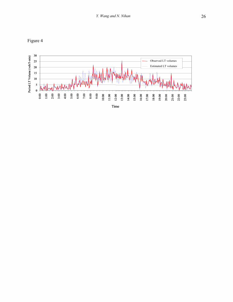
were 24-hour single-loop measurements, dated Thursday, May 13, 1999. Figure 4 shows the

comparison between the LT volumes observed by the dual loop and those estimated by the

proposed algorithm using single-loop measurements for each time period. In general, the two

curves fit well, especially during nighttime and early morning stretches. The correlation

coefficient between the two time series is 0.83, showing that they are well synchronized.

Comparisons of the two LT volumes are summarized in Table 3.

FIGURE 4. Comparison of dual-loop observed LT volumes and those estimated by the proposed

algorithm.

TABLE 3. Comparisons between the Observed LT Volumes and Estimated LT Volumes

As the dual-loop observed 24-hour volume of 28,060 is smaller than the single-loop observed

volume of 28,302, the difference in sums in Table 3 may be exaggerated. In fact, the two single

loops that form the dual loop, ES-163R: MMS___3 and ES-163R: MMS__S3, observed almost

the same volume − 28,302 and 28,325, respectively. Thus, the dual loop probably discarded

some vehicles from its volume count. This happens when the dual loop flags an error in the

length or speed calculation and drops the detected vehicle from calculation. LTs are judged to be

the most likely vehicles to activate such flags. If LTs have a higher probability of causing dual-

loop malfunctions, and hence are discarded, the difference between the estimated LT volume and

ground truth data should be even smaller than that shown in Table 3. However, further study is

needed to verify this. Video ground truth data could aid such verification and provide closer

evaluation results.


FIGURE 5. LT volume estimation error and total vehicle volume curves.

Figure 5 shows the estimation error (denoted by ε defined as the estimated LT volume minus the

dual-loop observed LT volume) and single-loop-observed total vehicle volume for each time

period. Statistics for estimation errors are summarized in Table 4. Due to the fluctuation of

traffic volumes and the tiny difference in segmentation time between single-loop and dual-loop

detectors, the variation of the error curve within a small range should be normal. In Figure 5,

however, while estimation errors are very close to 0 under low volume (less than 100veh/5min,

or 1200vph) conditions, the proposed algorithm overestimates LT volumes when traffic volume

is heavy (over 150veh/5min or 1800vph). This is probably due to the fact that when traffic

volume is heavy, speed is very unstable, and the uniform speed assumption is seriously violated.

The lengthened occupancies caused by slower speeds were attributed to longer vehicle lengths

and, therefore, LT volumes were overestimated. On the other hand, there were two periods, one

at 9:45am and the other at 2:30pm, with LT volumes significantly underestimated by the

algorithm. By checking the dual-loop measurements of the periods, the underestimations were

found caused by violations of the second assumption, i.e., there was no interval or only one

interval was LT-free for each of the two periods. Under such cases, the algorithm will mistakenly

regard occupancy for intervals with LTs as SV occupancy, and hence real vehicle lengths will be

shortened correspondingly in the calculation. However, the probability of such violations can be

very rare if period length is properly chosen.

TABLE 4. Statistics of Estimation Errors


In general, the proposed algorithm works better under un-congested conditions as shown by the

statistics in Table 4. When traffic volume is heavy, estimation errors may be enlarged. For the

studied data, relative estimation errors shown in the bottom row of Table 4 were within 8% even

for conditions with high traffic volume. This indicates that the proposed algorithm works

reasonably well under low, moderate, and reasonably high, yet still stable, traffic conditions.

However, if traffic is under stop-and-go conditions, the algorithm will not be applicable due to

the serious violations of its fundamental assumptions.

CONCLUSION

LT volume data are important for many purposes in transportation planning and engineering. As

LT travel patterns are season-dependent, data obtained by surveys conducted for a short period

of time every one to three years may not be sufficient for adequate safety planning, traffic

management and infrastructure maintenance. Though dual-loop detectors provide comparatively

reliable real-time measurements of volume for each classification, they are still not as commonly

available as single-loop detectors. Therefore, making single loops capable of providing LT

volume data is a very significant goal for practice as well as for research and development of

ATMS systems.

In this paper, an algorithm to estimate LT volume using only single-loop outputs was presented.

A computer program that implements the algorithm was developed in this study. To run the

program, a few parameters, i.e., single-loop length, mean and variance of SV length, and mean


and variance of LT length, need to be identified. The program takes in single-loop measurements

and outputs LT volume for each time interval. Pattern discrimination was used to separate

intervals with possible LTs from those without LTs. For the intervals with possible LTs, the NN

decision rule was applied to the interval's characteristics (as measured by single-loop data), to

assign it to one of the predefined vehicle composition categories. Once the nearest category is

identified, LT volume is automatically estimated.

The LT volumes estimated by the proposed algorithm were compared to those observed by dual-

loop detectors. The two LT volume series fit very well, especially when traffic volume was low.

If single-loop data are input in real time, the program will give real-time LT volumes. This will

be very valuable for dynamic traffic control and management.

Possible estimation errors in using the algorithm were also discussed. To avoid overestimation

and underestimation of the LT volumes, two fundamental assumptions, i.e., uniform speed

within each period, and at least two intervals per period have no LTs present, must be met. Under

the current status, the program is not capable of checking the satisfaction of the two fundamental

assumptions automatically. Also, quantitative effects of the violations of the two fundamental

assumptions on the estimation results are unclear. Future research will specifically address these

problems and widely check the transferability of the algorithm to other sites in order to make the

proposed method more complete and robust.


REFERENCES

Coifman, B. (1998). Vehicle reidentification and travel time measurement in real-time on

freeways using the existing loop detector infrastructure, Transportation Research Record 1643,

TRB, National Research Council, Washington, D.C., 181-191.

Cover, T. M., and Hart, P. E. (1967). Nearest neighbor pattern classification. IEEE Transactions

on Information Theory, Vol. IT-13, No. 1, 21-27.

Cunagin, W. D., and Messer, C. J. (1983). Passenger car equivalents for rural highways.

Transportation Research Record 905, TRB, National Research Council, Washington, D.C., 61-

68.

Dudani, S. A. (1976). The Distance-Weighted K-Nearest-Neighbor Rule. IEEE Transactions on

Systems, Man, and Cybernetics, Vol. SMC-6, No. 4, 325-327.

Garber, N. J., and Joshua, S. (1989). Characteristics of large-truck crashes in Virginia,

Transportation Quarterly, Vol. 43, No. 1, 123-138.

Hallenbeck, M. (1993). Seasonal truck volume patterns in Washington State. Transportation

Research Record 1397, TRB, National Research Council, Washington, D.C., 63-67.

Hutchinson, B. G. (1990). Large-truck properties and highway design criteria. Journal of

Transportation Engineering, Vol. 116, No. 1, 1-22.

Ishimaru, J. M., and Hallenbeck, M. E. (1999). Flow Evaluation Design Technical Report,

Technical Report WA-RD 466.2, Washington Department of Transportation, Seattle.

Keller, J. M., Gary, M. R., and Givens, J. A. Jr. (1985). A fuzzy K-nearest neighbor algorithm.

IEEE Transactions on Systems, Man, and Cybernetics, Vol. SMC-17, No. 4, 580-585.


Nihan, N. L., Leth, M., and Wong, A. (1995). Video Image Processing for Freeway Monitoring

and Control: Evaluation of the Mobilizer. Technical Report WA-RD 398.1, Washington

Department of Transportation, Seattle.

Sun, C., Ritchie, S. G., and Jayakrishnan, R. (1999). Use of vehicle signature analysis and

lexicographic optimization for vehicle reidentification on freeways, Transportation Research,

part c, Vol. 7, No. 4, 167-185.

Transportation Research Board, National Research Council. (1998). Special Report 209:

Highway Capacity Manual, 3rd ed. Washington, D.C.

Wang, Y., and Nihan, N. L. (2002). A Robust Method of Filtering Single-Loop Data for

Improved Speed Estimation. Preprint CD-ROM, the 81st Annual Meeting of Transportation

Research Board, Washington, D.C.

Wang, Y., and Nihan, N. L. (2000). Freeway traffic speed estimation using single loop outputs,

Transportation Research Record, 1727, TRB, National Research Council, Washington, D.C.,

120-126.


List of Figures:

FIGURE 1. Snapshot of southbound I-5 at NE 130th Street.

FIGURE 2. Length distribution of vehicles on southbound I-5

FIGURE 3. Vehicle length distributions with normal distribution curves

FIGURE 4. Comparison of dual-loop observed LT volumes and those estimated by the proposed

algorithm.

FIGURE 5. LT volume estimation error and total vehicle volume curves.


Figure1

GP Lane 3 GP Lane 2

GP Lane 1GP Lane 4

HOV Lane

GP Lane 3 GP Lane 2

GP Lane 1GP Lane 4

HOV Lane


Figure 2

29.527.5

25.523.4

31.419.4

17.315.3

13.311.2

9.27.15.13.11.1

SVs LTs

60

50

40

30

20

10

0

Freq

uenc

y (p

erce

nt)

Length in meter

29.527.5

25.523.4

31.419.4

17.315.3

13.311.2

9.27.15.13.11.1

SVs LTs

60

50

40

30

20

10

0

Freq

uenc

y (p

erce

nt)

Length in meter


Figure 3

(a) SV ClassVehicle Length (m)

12.09.06.03.0

Freq

uenc

y (p

erce

nt)

0.0

10.0

20.0

30.0

40.0 Normal curve

(b) LT ClassVehicle Length (m)

302724211815120.0

10.0

20.0

Freq

uenc

y (p

erce

nt)

Normal curve

(a) SV ClassVehicle Length (m)

12.09.06.03.0

Freq

uenc

y (p

erce

nt)

0.0

10.0

20.0

30.0

40.0 Normal curve

(b) LT ClassVehicle Length (m)

302724211815120.0

10.0

20.0

Freq

uenc

y (p

erce

nt)

Normal curve


Figure 4

0

5

10

15

20

25

30

0:00

1:00

2:00

3:00

4:00

5:00

6:00

7:00

8:00

9:00

10:0

0

11:0

0

12:0

0

13:0

0

14:0

0

15:0

0

16:0

0

17:0

0

18:0

0

19:0

0

20:0

0

21:0

0

22:0

0

23:0

0

Time

Perio

d LT

Vol

ume

(veh

/5-m

in)

Observed LT volumes

Estimated LT volumes

0

5

10

15

20

25

30

0:00

1:00

2:00

3:00

4:00

5:00

6:00

7:00

8:00

9:00

10:0

0

11:0

0

12:0

0

13:0

0

14:0

0

15:0

0

16:0

0

17:0

0

18:0

0

19:0

0

20:0

0

21:0

0

22:0

0

23:0

0

Time

Perio

d LT

Vol

ume

(veh

/5-m

in)

Observed LT volumes


Observed LT volumes



Figure 5

Estim

atio

n Er

ror ε

(LTs

per p

erio

d)

0

50

100

150

200

0:00

1:00

2:00

3:00

4:00

5:00

6:00

7:00

8:00

9:00

10:0

0

11:0

0

12:0

0

13:0

0

14:0

0

15:0

0

16:0

0

17:0

0

18:0

0

19:0

0

20:0

0

21:0

0

22:0

0

23:0

0

Time

Perio

d V

ehic

le V

olum

e(v

eh/5

-min

)

-20-1001020304050

Volume

Error

Estim

atio

n Er

ror ε

(LTs

per p

erio

d)

0

50

100

150

200

0:00

1:00

2:00

3:00

4:00

5:00

6:00

7:00

8:00

9:00

10:0

0

11:0

0

12:0

0

13:0

0

14:0

0

15:0

0

16:0

0

17:0

0

18:0

0

19:0

0

20:0

0

21:0

0

22:0

0

23:0

0

Time

Perio

d V

ehic

le V

olum

e(v

eh/5

-min

)

-20-1001020304050

Volume

Error


List of Tables:

TABLE 1. Four Length-Based Vehicle Categories Used by the WSDOT

TABLE 2. Descriptive Statistics of Dual-Loop Measured Vehicle Lengths

TABLE 3. Comparisons between the Observed LT Volumes and Estimated LT Volumes

TABLE 4. Statistics of Estimation Errors


Table1 TABLE 1. Four Length-Based Vehicle Categories Used by the WSDOT Classes Range of length (meter) Vehicle types Bin1 Less than 7.92 Cars, pickups, and short single-unit trucks Bin2 From 7.93 to 11.89 Cars and trucks pulling trailers, long single-unit trucks Bin3 From 11.90 to 19.81 Combination trucks Bin4 Longer than 19,82 Multi-trailer trucks


Table 2 TABLE 2. Descriptive Statistics of Dual-Loop Measured Vehicle Lengths Class Number of Cases Mean Std Deviation Minimum Maximum SV (Bin1 + Bin2) 4443 5.48m 0.87m 1.83m 11.89m LT (Bin3 + Bin4) 472 22.50m 3.59m 12.19m 30.17m


Table 3 TABLE 3. Comparisons between the Observed LT Volumes and Estimated LT Volumes

Minimum Maximum Mean Median Std Dev. Sum Observed 5-min LT Volume 0 25 7.12 6 5.24 2050 Estimated 5-min LT Volume 0 26 7.49 7 4.77 2156


Table 4 TABLE 4. Statistics of Estimation Errors

Period volume conditions (veh/5min) Less than 50 Between 50 and 100 More than 100 All conditions

Case No. 122 55 166 288E(ε) * (veh/5min) -0.098 -0.146 0.711 0.368σ(ε) ** (veh/5min) 0.827 1.026 3.742 2.915E(LTs) (veh/5min) 2.373 4.636 9.855 7.118E(ε) / E(LTs) -0.041 -0.031 0.072 0.052

* E(⋅) indicates the expectation of the variable in the parentheses. ** σ (⋅) indicates the standard deviation of the variable in the parentheses.


Author biography: Dr. Yinhai Wang is a Research Assistant Professor of Civil and Environmental Engineering at the University of Washington. He has a Ph.D. in transportation engineering, a master’s degree in computer science, another master’s degree in construction management, and a bachelor degree in civil engineering. Dr. Wang established the TransNow (Transportation Northwest) ITS Program at the University of Washington and serves as the Program coordinator. Dr. Wang has conducted extensive research in loop data application, traffic accident modeling, image processing, and vehicle tracking. Nancy L. Nihan is a Professor of Civil and Environmental Engineering at the University of Washington in Seattle and also serves as the Director of Transportation Northwest (TransNow), which is the University Transportation Center for Federal Region 10. Prior to joining the UW, Professor Nihan had a joint appointment with the Department of Systems Engineering and the Center for Urban Studies at the University of Illinois, Chicago Circle Campus. Dr. Nihan's degrees include the B.S.I.E. from the Department of Industrial Engineering, Northwestern University, Evanston Illinois and the Masters and PhD degrees from the Department of Civil Engineering at NU.

Dynamic Estimation of Freeway Large-Truck Volumes Based on Single-Loop Measurements

Documents

Transcript of Dynamic Estimation of Freeway Large-Truck Volumes Based on Single-Loop Measurements