Dynamic Effects of Terms of Trade Shocks: The Impact on Debt and Growth

Theo S. Eicher University of Washington, Seattle

Ifo Institute at the Ludwig-Maximilians-Universität München

Stefan F. Schubert Free University of Bozen-Bolzano

Stephen J. Turnovsky University of Washington, Seattle

The recent empirical literature on the economic effects of terms of trade shocks highlights not only the direct effects on growth, but also the resulting changes in volatility and debt. We link the procyclicality of sovereign debt to terms of trade shocks and provide theoretical underpinnings for standby facilities such as the “Exogenous Shocks Facility” recently created by the IMF. By modeling international capital market imperfections and changes in creditworthiness during adverse terms of trade shocks, we show that transitions can involve excessive adjustment as debt decumulation overshoots its long run equilibrium to prolong the adjustment recession. Our model adds a novel dynamic dimension to the Harberger-Laursen-Metzler effect. In contrast to the previous terms of trade literature, we highlight that the precise nature of the capital imperfection is key to the results. When credit depends not on the level of debt but on the debt to equity ratio the model naturally features dynamic effects that are not found in previous models. It also highlights that how a country responds to terms of trade shocks depends importantly on whether the country is a creditor or debtor. Finally we assess the welfare costs associated with terms of trade shocks. For plausible parameterizations we find that a 20 percent deterioration in the terms of trade may lead to a welfare loss on the order of 10 to 15 percent.

July 2006

1

1. Introduction

Adverse shocks to a country’s terms of trade – the relative price of its exports to imports –

not only may disrupt the economy’s growth, but also may introduce considerable instability. The

impacts of such shocks have been extensively documented. For example, Mendoza (1995) and Kose

(2002) find that terms of trade shocks account for at least half of the output volatility in developing

countries, while Barro (1996) documents that sustained deteriorations in a country’s terms of trade

can have a significantly negative impact on growth.1 Recent empirical evidence links terms of trade

shocks not only to changes in economic growth and volatility, but also to changes in borrowing

premiums and to the severity of debt crises.2 This link has not been modeled formally, and in this

paper we examine specifically how the effects of terms of trade shocks on growth and instability are

influenced by debt and international capital flows.

The effects of terms of trade shocks on a small open economy have been extensively studied

since the early 1950’s when Harberger (1950) and Laursen and Metzler (1950) predicted that a

deterioration in the terms of trade would reduce real income, thereby lowering savings and

investment to cause a deterioration of the current account balance. The “Harberger-Laursen-Metzler

effect” is purely static, however, giving rise to an extensive literature that re-examined the effects of

terms of trade shocks within an intertemporal framework.3 One general conclusion of the

intertemporal literature is that the Harberger-Laursen-Metzler effect is sensitive to several key

features of the economy. These include the exact specification of the nature of the (i) preferences

(Obstfeld, 1982, Svensson and Razin, 1983, Mansoorian, 1993, Ikeda, 2001); (ii) production in

terms of labor supply (Bean, 1986) and capital (Sen and Turnovsky, 1989); (iii) international capital

market imperfections (Obstfeld, 1982, Huang and Meng, 2006); and (iv) duration of the shock

1 Mendoza (1995) finds that terms of trade disturbances explain 56 percent of aggregate output fluctuations in developing countries. Kose (2002) studies a broader set of world price shocks (including intermediate and primary goods) to find that they explain roughly 88 percent of aggregate output fluctuations. Turnovsky and Chattopadhyay (2003) provide evidence to show that volatility in the terms of trade have adverse effects on the growth rate. 2 See Min (1998), Min et. al. (2003), Cuadra and Sapriza (2006) and Peter (2002) for a survey on econometric studies of the probability of sovereign default in emerging markets. 3 This reappraisal was initiated by Obstfeld (1982) and further pursued in a number of different directions by Svensson and Razin (1983), Persson and Svensson (1985), Bean (1986), and Sen and Turnovsky (1989), and more recently by Serven (1999), Ikeda (2001), Otto (2003), and Huang and Meng (2004). See Duncan (2003) for a survey.

2

(Obstfeld, 1982, Persson and Svensson, 1985).

Previous investigations of the link between capital market imperfections and terms of trade

shocks have been motivated by the potential for financial flows to smooth consumption following

adverse shocks. However, this would imply that debt flows are countercyclical, contradicting the

data that clearly suggests that debt flows are procyclical.4 This procyclicality is thought to be driven

by external supply factors that amplify the impact of the initial shock and exacerbate growth booms

and busts. One such factor that has been closely tied in the data to procyclicality is the change in

risk perception on the part of creditors (see, e.g., Kaminsky, Reinhart, and Végh 2003). Specifically,

it is thought that frequently updated credit ratings influence the quantity and the price of

international capital. Under such circumstances procyclical capital flows attract unsustainably large

capital inflows during favorable shocks and force countries to overadjust to adverse shocks (see

World Bank 1993, p. 20 and Easterly, Islam, and Stiglitz 1999).

In this paper we seek to model such adjustment dynamics to terms of trade shocks. We

extend a simple growth model to incorporate the role of endogenous country-specific borrowing

premiums. The objective is to examine the resulting debt flows to see if these external factors

amplify contractions (expansions) in the case of adverse (favorable) terms of trade shocks. Interest

in the interplay between terms of trade shocks, risk, debt, and growth has gained significant

momentum since the Asian crisis. Broda and Tille (2003) provide an extensive survey to show how

strongly terms of trade, debt, growth, and risk are linked in developing countries. Min (1998) and

Min, et. al. (2003) find that worsening terms of trade are associated with higher yield spreads, which

is a key element of our model below. Terms of trade shocks have also been closely linked to

changes in capital flows by Caballero and Panageas (2003), and Calvo, Izquierdo, and Mejia (2004),

who find that negative terms of trade shocks increase the likelihood of a sudden stop in capital

inflows and large interest rate upswings. This evidence is consistent with the findings in Broda

4 Procyclicality of capital flows to developing countries was first documented by Díaz-Alejandro, (1983) and (1984) prior to the first Latin American debt crisis. For recent, systematic reviews of the evidence on the procyclicality of capital flows, see Dadush, Dasgupta, and Ratha (2000), and Kaminsky, Reinhart, and Végh (2003). Procyclicality is observed not only for terms of trade shocks, but also for cyclical growth swings; see Botman, Dasgupta, and Ratha (1999).

3

(2004) and Broda and Tille (2003), who observe that most crises are preceded by negative terms of

trade shocks that caused substantial economic fluctuations and disruption to output growth.

By focusing on the response of capital flows to terms of trade shocks we are extending the

Harberger-Laursen-Metzler literature in four important directions. First, we focus on a growing

developing country that is facing an imperfect capital market, in contrast to most of the literature

cited above, which assumes perfect world capital markets. Indeed, problems stemming from

deteriorations in terms of trade are likely to be more serious for developing economies that face

restricted access to world financial markets.

Second, we highlight how important the precise nature of the capital market imperfection is

for its consequences for the economy. Previous authors have specified the borrowing cost to

increase with the nation’s level of debt. This specification, together with a constant rate of time

preference and inelastic labor supply, implies that terms of trade shocks have no dynamic effects.

The only response is that consumption fully adjusts instantaneously, with the current account

remaining unchanged.5 But in reality the borrowing premium depends not on the nation’s level of

absolute debt, but rather its ability to finance its debt, a measure that can be conveniently proxied by

the country’s debt to equity ratio. 6 In this case, our model generates implications that can serve as

theoretical underpinnings for the observed growth, risk and debt dynamics of developing countries.

Adverse terms of trade shocks lead to transitions that involve recessions and procyclical debt

adjustments. The debt adjustment may even be excessive, in that the debt level may overshoot its

long-run equilibrium during the transitions. In addition, we show that financial markets can prolong

terms of trade induced recessions. The adverse changes in the borrowing risk premium can force

countries to pay down debt further and faster than necessary to lower the borrowing costs and

jumpstart investment again. We therefore find ample justification for terms of trade adjustment

facilities such as the IMF’s “Exogenous Shocks Facility” introduced in 2005.

5 Dynamics can be restored by modifying the specification of preferences, although this may or may not be consistent with the HLM condition; see Obstfeld (1982) and Huang and Meng (2004). 6 See Edwards (1984), Chatterjee, Sakoulis, and Turnovsky (2003), and footnote 10. It may also be necessary if one is to generate a long-run balanced growth path, along which debt, capital, and output all grow at a common rate while the rate of return remains constant.

4

A third novel result is that the current account response to a terms of trade shock is shown to

depend critically on a country’s credit status – i.e., whether it is a debtor or creditor. In the former

case, we find that an adverse terms of trade shock leads to a decline in growth accompanied by a

pro-cyclical decline in debt that causes an improvement in the current account, contradicting the

Harberger-Laursen-Metzler proposition. In the latter case, we find the opposite; an increase in

growth together with a decrease in the holdings of foreign assets, consistent with Harberger-

Laursen-Metzler.

The Harberger-Laursen-Metzler literature can also be interpreted as implicitly involving

welfare judgments, where welfare is proxied by measures such as expenditures and current account

balances.7 Our fourth contribution is to assess the welfare costs explicitly, by evaluating the effect

of terms of trade changes on the consumer’s intertemporal utility as the economy transitions to its

equilibrium path. We show that an adverse terms of trade shock generates both a negative income

effect and a wealth effect that is negative, and therefore reinforcing for a debtor country, but

positive, and therefore offsetting, for a creditor econom. For a plausible parameterization we find

that a 20 percent deterioration in the terms of trade may lead to a welfare loss on the order of 10 to

15 percent in equivalent variation consumption flows, depending upon the chosen consumption mix.

Interestingly, our simulations indicate that the magnitude of the wealth effect is reduced as capital

market imperfections increase because the economy is less reliant on foreign financing in the initial

equilibrium – which reduces the impact of a terms of trade shock.

The remainder of the paper proceeds as follows. Section 2 sets out the analytical framework,

while Section 3 derives the macroeconomic dynamic equilibrium. Because of the complexity of the

model it is necessary to resort to numerical simulations and these are conducted in Section 4, while

Section 5 concludes.

2. Analytical Framework

7 Two exceptions to this should be noted. Svensson and Razin (1983) use duality theory to obtain welfare effects of terms of trade disturbances in a two period analysis, while Turnovsky (1993) assesses the welfare effects of terms of trade shocks in a stochastic AK growth model in which the economy is always on its stochastic balanced growth path.

5

To incorporate movements in the terms of trade, we extend the one-sector “non-scale”

growth model of Eicher and Turnovsky (1999a) to include foreign imports.8 We consider a small

open economy that produces a traded commodity, X, and that imports a foreign good, Z, the relative

price of which is expressed in terms of the foreign good, X Zp p p= . The economy is small, in the

sense that relative goods prices are fixed in the world market. We assume that p remains constant

and analyze the consequences of a one-time unanticipated permanent change in p. Identical

individuals’ labor supply, Li , is fixed and full employment implies that the total labor supply equals

the population size, N. The population growth rate is /N N n= . Each individual produces domestic

output, Yi , using private capital, Ki , and labor, Li .

1i i i iY L K K K Kσ σ η σ ηα α−′= ≡ 0 < σ <1, η <

> 0 (1a)

We allow for spillovers from the aggregate economy-wide capital stock, iK NK≡ , as in Romer

(1986).9 In addition, we assume constant returns in the two private factors, but total returns to scale

of 1 + η in all factors. Aggregate returns to scale are thus increasing or decreasing, depending on

the qualitative nature of the spillovers on private production.

Each agent’s utility is represented by the intertemporal isoelastic utility function

( )0

11 ; 1; 0 1ti iX Z e dt

γθ θ ρ γ θγ

∞ − −Ω ≡ −∞ < < < <∫ (1b)

where )1(1 γδ −≡ equals the intertemporal elasticity of substitution, and θ represents the relative

importance of the domestic good in utility.

Agents accumulate physical capital, with expenditure on a given change in the capital stock,

Ii , involving adjustment (installation) costs that we incorporate in the quadratic (convex) function

Φ(Ii , Ki ) = Ii + hIi

2

2Ki

= Ii 1+h2

Ii

Ki

⎛

⎝ ⎜ ⎞

⎠ ⎟

8 The “non-scale” growth model is a generalization of the neoclassical growth model to allow for non-constant returns to scale. It was pioneered by Jones (1995a, 1995b), under the label “semi-endogenous” growth model, as an effort to respond to some of the counter-factual implications carried by first generation endogenous growth models. 9 Such spillovers have been motivated in various ways. One is to interpret K as knowledge capital, another is to assume N specific inputs (subscripted by i), in which case intra-industry spillovers of knowledge are represented by aggregate K. Alternatively, a negative spillover can be viewed as reflecting congestion, as in Barro and Sala-i-Martin (1992).

6

This equation is an application of the familiar Hayashi (1982) cost of adjustment framework, where

we assume that the adjustment costs are proportional to the rate of investment per unit of installed

capital (rather than its level). The linear homogeneity of this function is necessary if a steady-state

equilibrium having ongoing growth is to be sustained. For simplicity, we assume that the capital

stock does not depreciate, so that the net rate of capital accumulation is given by:

i i iK I nK= − (1c)

In addition to importing a foreign consumption good, domestic agents have access to a world

capital market, allowing them to borrow internationally. Aside from the compelling empirical

observations stressing how terms of trade shocks affect developing economies, the literature on pro-

cyclicality of debt movements clearly highlights the importance of imperfect access to capital

markets for non-OECD countries. Terms of trade crises have become intimately linked not only to

deteriorating value of export production, but also to skyrocketing debt and significant borrowing

premiums. We incorporate this credit feature explicitly into our model.

We assume that the creditworthiness of the economy influences its cost of borrowing from

abroad. The world capital market assesses the economy's ability to service its debt costs, and views

the country's debt-capital (equity) ratio as an indicator of its potential default risk. Accordingly, the

interest rate a country is charged on the world capital market increases with this ratio. This leads to

an upward-sloping supply schedule for debt, which we express by assuming that the borrowing rate,

( )r B pK , charged on (national) foreign debt, B, relative to the value of private capital, pK, is of the

form:

( ) ( )* ; >0, >0r B pK r B pKω ω ω′ ′′= + (1d)

where r* is a world interest rate (for example the LIBOR) and [ ]B pKω is the country-specific

borrowing premium.10

10 Various formulations of (1d) can be found in the literature. The original formulation by Bardhan (1967) expressed the borrowing premium in terms of the absolute stock of debt; see also Obstfeld (1982), and Bhandari, Haque, and Turnovsky (1990). Other authors, such as Cooper and Sachs (1985) argued that a country can shift the upward-sloping supply function outward by adopting growth-oriented policies, so that a lower borrowing premium is charged for each level of debt. This can be incorporated by assuming that the borrowing premium depends upon the level of debt relative

7

The representative agent’s objective is to choose consumption of the two goods, a rate of

investment, and his rate of accumulation of debt, so as to maximize intertemporal utility (1b) subject

to the capital accumulation constraint, (1b), and flow budget constraint, expressed in terms of the

foreign good:11

[ ]( ) iiiiiii BnpKBrYKIpZXpB ⎟⎟

⎠

⎞⎜⎜⎝

⎛−⎥

⎦

⎤⎢⎣

⎡+−Φ++= ,/ (1e)

In performing this optimization, each individual agent takes the borrowing rate, [].r , as given since

the interest rate as specified in (1d) is a function of the economy's aggregate debt-capital ratio.

The optimality conditions with respect to the two consumption goods and investment are

1 (1 )i iX Z pθγ γ θθ λ− − = (2a)

(1 ) 1(1 ) i iX Zθγ γ θθ λ− −− = (2b)

( )( )1 i ih I K q+ = (2c)

Where λ is the shadow value (marginal utility) of wealth in the form of internationally traded debt

and q is the value of capital in terms of the (unitary) price of foreign bonds.12 The first two

conditions equate the marginal utility of consumption to the marginal utility of wealth in terms of the

domestic and the imported goods, respectively.

From the static optimality conditions (2a) and (2b), we can examine how domestic and

foreign good consumption vary with value of foreign assets and the terms of trade, namely

1 1 (1 )(1 ) (1 )

i

i

dX d dpX p

λ γ θγ λ γ

− −= − −

− − (3a)

to some measure of earning capacity (or debt-servicing capacity) such as capital, or output. This latter formulation is the one we have adopted; it has been previously used by van der Ploeg (1996). Imposing convexity of the function is a convenient way to parameterize the borrowing ceiling as specified by Eaton and Gersovitz (1981). 11 Since we are focusing primarily on debtor nations, we assume B > 0. However, it is possible for B < 0, in which case the agent accumulates credit by lending abroad. 12 Strictly speaking, the shadow values , qλ pertain to individuals and should carry subscripts i. Since agents are identical, the shadow values are identical, and we suppress them for notational expedience.

8

1(1 ) (1 )

i

i

dZ d dpZ p

λ γθγ λ γ

= − −− −

(3b)

An increase in the shadow value of foreign assets raises the cost of foreign debt and thus the

marginal utility of debt reduction. In response, consumption of both goods is reduced in an effort to

buy down foreign debt. A deterioration in the relative price of the domestic good (i.e., a drop in p)

has two effects. First, a substitution effect induces consumers to switch their consumption from

foreign to the relatively cheaper domestic good. The second effect is the associated income effect,

as the marginal utility of debt reduction in terms of the domestic good falls, which increases

consumption of both goods. The effect of the deterioration in the terms of trade is thus

unambiguously positive for the domestic good but positive or negative for the foreign good,

depending on whether or not the intertemporal elasticity of substitution exceeds unity. In the case of

log utility, 0γ = , the income and substitution effects are precisely offsetting and the consumption of

the imported good is unchanged. Letting

i i iC pX Z≡ + (4)

denote the total consumption of agent i (expressed in terms of the foreign good), and dividing (2a)

by (2b), yields

i ipX Cθ= , (1 )i iZ Cθ= − (4’)

implying that imports and domestic goods are consumed in proportion to their terms of trade

weighted share, , 1θ θ− , in the utility function.

Equation (2c) equates the marginal cost of capital to its market value. Combining this

equation with the accumulation constraint (1c) immediately implies a growth rate that is dependent

on the relative price of domestically installed capital

1i i

i i

K I qn nK K h

−= − = − (5)

The optimality conditions with respect to the rate of accumulation of debt and physical

9

capital are summarized by the arbitrage conditions

Br npK

λρλ

⎡ ⎤− = −⎢ ⎥

⎣ ⎦ (6a)

2( 1)

2i

i

Y q q BrqK q hq pKσ ⎡ ⎤−

+ + = ⎢ ⎥⎣ ⎦

(6b)

Equations (6a) and (6b) equate the cost of debt to the rates of return on consumption and domestic

capital accumulation, respectively. The return to domestic capital consists of three components.

The first is output per unit of installed capital (valued at the price q), while the second term is the

rate of capital gain. The third element reflects the fact that an additional benefit of a higher capital

stock is to reduce the installation costs (which depend upon Ii Ki ) associated with new investment.

Finally, to ensure that the agent's intertemporal budget constraint is met, the following

transversality conditions must be imposed:13

0limlim == −

∞→

−

∞→

tit

tit

eKqpeB ρρ λλ (6c)

3. Aggregate Dynamics

Our objective is to analyze the dynamics of the aggregate economy about a stationary growth

path in response to an exogenous terms of trade shock. Along such an equilibrium path, aggregate

output and the aggregate capital stock are assumed to grow at the same constant rate, so that the

aggregate capital-output ratio remains constant. Summing the individual production functions over

the N agents, yields the aggregate production function

NK NKNKY σσσση αα ≡= −+ 1 (7)

where σ N ≡1 − σ is the share of labor in aggregate output, σK ≡ σ + η is the share of capital in

aggregate output, and the total returns to scale are given by σK + σ N = 1+ η . Taking percentage

changes of (7) and imposing the long-run condition of a constant Y K ratio, the equilibrium long-

run growth of capital and output, g, is given by

13The transversality condition on debt is equivalent to the national intertemporal budget constraint.

10

1

N

K

g nσσ

≡−

(8)

The equilibrium growth rate in (8) thus depends on the aggregate returns to scale and the rate of

population growth. The growth rate is positive if and only if 1<Kσ . Under constant returns to

scale, the rate of growth of the economy equals the rate of population growth, g = n . Otherwise, g

exceeds n, or is less than n -- that is, there is positive or negative per capita growth, according to

whether returns to scale are increasing or decreasing, η <> 0.

Taking the time derivative of iK NK≡ and summing (5) over the N identical individuals, the

growth rate of the aggregate capital stock is given by

1K qK h

−= (9a)

Similarly, taking the time derivative of iB NB≡ and summing over (1e), yields the accumulation of

the aggregate debt

BpKBrYK

hq

pCpB ⎥

⎦

⎤⎢⎣

⎡+⎟⎟

⎠

⎞⎜⎜⎝

⎛−⎟⎟

⎠

⎞⎜⎜⎝

⎛ −+=

212

(9b)

Finally, taking the time derivatives of (i) iC NC≡ , (2b) and (4’), while also noting (6a), the growth

rate of aggregate consumption is thus given by

[ ]1

r B pK nCC

ρ γγ− −

=−

(9c)

Comparing (9a) with (9c), we see that while the former depends upon production conditions, as

reflected in q, the latter depends upon taste parameters and borrowing costs, as reflected in (.)r ; see

Turnovsky (1996).

To analyze the transitional dynamic evolution of the aggregate economy about its stationary

equilibrium growth path, it is convenient to express the system in terms of the relative price of

capital, q, and the following stationary variables

11

( ) ( ) ( )(1 ) (1 ) (1 ) ; ; ; N K N K N K

K B Ck b cN N Nσ σ σ σ σ σ− − −

≡ ≡ ≡ (10)

In the absence of any productive externality, 1K Nσ σ+ = and the quantities in (9) reduce to standard

per capita quantities. Otherwise, we shall refer to them as “scale-adjusted” per capita quantities; see

Eicher and Turnovsky (1999a, 1999b).

Taking the time derivatives of these quantities, we may summarize the macrodynamic

equilibrium by

1k q gk h

−= − (11a)

[ ]( )2 12

Kb p c qr b pk g k kb b p h

σα⎛ ⎞⎛ ⎞−

= − + + −⎜ ⎟⎜ ⎟⎝ ⎠⎝ ⎠

(11b)

2

1( 1)2

Kb qq r q kpk h

σασ −⎡ ⎤ −= − −⎢ ⎥

⎣ ⎦ (11c)

[ ]1

r b pk nc gc

ρ γγ− −

= −−

(11d)

Equations (11a) – (11d) provide an autonomous set of dynamic equations in , , ,k b q c , from which

the dynamic time paths of other variables can be inferred.14

3.1. Steady State

The steady state equilibrium to this economy is attained when 0c k b q= = = = , so that the

corresponding stationary values, denoted by tildes, are determined by

1q gh= + (12a)

( )2 1 02

Kc qr g b p k kp h

σα⎛ ⎞⎛ ⎞−

− + + − =⎜ ⎟⎜ ⎟⎝ ⎠⎝ ⎠

(12b)

14 It is apparent from the structure of system (11) that a debt supply function of the form ( )r r B= would be inconsistent with a long-run balanced growth equilibrium.

12

2

1( 1) 02

Kqrq k

hσασ −−

− − = (12c)

1

r n gρ γγ

− −=

− (12d)

*r r b pk r b pkω⎡ ⎤ ⎡ ⎤= ≡ +⎣ ⎦ ⎣ ⎦ (12e)

This steady state has a simple recursive structure. First, equation (12a) determines the

steady-state price of installed capital, q , so that the equilibrium growth rate of capital equals the

equilibrium growth rate, g. Second, (12d) determines the country’s borrowing rate r such that the

equilibrium growth rate of consumption equals g. As a consequence, r depends upon the taste

parameters, ρ γ , and the technological parameters, σ , η , embodied in g. It is independent of the

shape of the borrowing function, [.]r , which given r , determines the resulting debt to capital ratio,

b pk , from (12e). Having determined both ˜ q and r , (12c) determines the scale-adjusted capital-

labor ratio, ˜ k , such that the rate of return on capital equals the equilibrium cost of debt. This, too, is

independent of the shape of the debt supply function, [.]r , which therefore has no effect on the

production side of the domestic economy. Having determined the debt to capital ratio, b pk , from

(12e), and the capital-labor ratio, ˜ k , from (12c), the debt-labor ratio, b , then immediately follows.

In particular, (12d) and (12e) together imply that in the long run the country will be a debtor

economy or creditor economy, according as

*1 >(1 ) <1n rσρ γ γ

σ η⎧ ⎫⎛ ⎞−

+ + −⎨ ⎬⎜ ⎟− −⎝ ⎠⎩ ⎭ (13)

Finally, given ˜ q , r , b , and ˜ k , (12b) determines the equilibrium scale-adjusted per capita

consumption, ˜ c , so as to maintain current account balance.

The equilibrium growth rate must be consistent with the transversality condition. By direct

calculation, this can be shown to reduce to: r g> . Substituting from (12d), this can be expressed in

terms of exogenous parameters as:

(1 ) ( )nρ σ η ρ γ− > +

13

As long as this condition is met, the steady-state equilibrium is unique.

Our concern in this paper is with the impact of a deterioration in the terms of trade. From

(12a) – (12d), we see that

0dr dk dqdp dp dp

= = = , db dc dpc pb

= = (14)

In the long run, a deterioration in the terms of trade leads to a proportionate reduction in the

economy’s level of debt. Total output, capital stock, and the borrowing rate remain unchanged.15

Total consumption, measured in terms of foreign output, also declines proportionately although

when measured in terms of domestic output, c p , it remains unchanged.16 Steady state

consumption of the domestically produced good, x, remains constant, whereas consumption of the

imported good, z, falls.

3.2 Transitional Dynamics

Although (14) suggests that the long-run impacts of a terms of trade shock on the economy

are relatively isolated, they nevertheless lead to profound changes in a country’s investment,

production, and foreign borrowing during a transition phase, the welfare consequences of which are

quite significant. Eicher and Turnovsky (1999b) have shown that such transitions may take

considerable time in non-scale models such as this. At accepted convergence rates of between 2 and

10 percent, the transition impact will be significant for at least 10 to 30 years, compounding to

significant level effects. We therefore proceed to analyze the transitional phase, doing so by

examining the linearized approximation to (11), namely:

15 This is consistent with Sen and Turnovsky (1989). In their analysis, the effect of the terms of trade shock on real activity operates through the labor-leisure choice. With inelastic labor supply, there is no production effect, as in the present analysis. It is straightforward to show that if one were to endogenize labor supply in the present analysis, then a change in the terms of trade would generate production effects, analogous to those obtained by Sen and Turnovsky. 16 In the knife-edge case where the economy starts out with no initial debt, it does not accumulate any debt along the transitional path. In this case, the stock of debt remains zero and the only response is in consumption.

14

[ ] [ ]

[ ] [ ]

[ ]( )

[ ]( )

21

31

2

0 0 0

.. 1

.. 0

. .0 0

1 1

kh

r b pqk k kk a r ghpkb b b

r qq q qa r gpkc c c

r bc r cp k p kγ γ

⎛ ⎞⎜ ⎟⎜ ⎟⎜ ⎟′ ⎛ ⎞⎛ ⎞ −+ −⎜ ⎟⎜ ⎟⎜ ⎟⎜ ⎟ −⎜ ⎟⎜ ⎟ = ⎜ ⎟⎜ ⎟⎜ ⎟ ′ −⎜ ⎟− ⎜ ⎟⎜ ⎟⎜ ⎟ ⎜ ⎟⎜ ⎟ −⎝ ⎠ ⎝ ⎠⎜ ⎟′ ′⎜ ⎟−⎜ ⎟− −⎝ ⎠

(15)

where 2 2

121 2

( 1)2

KK

b qa r p p khpk

σασ −−′≡ − + − , [ ]231 2

.(1 ) K

K

r bqa k

pkσασ σ − ′

≡ − − .

This structure is virtually identical to that considered by Eicher and Turnovsky (1999a). There it

was shown that the system almost certainly has two positive and two negative eigenvalues,

arbitrarily ordered as 4321 0 µµµµ <<<< . A simple sufficient condition for this to be so is that

(1 )KC pY σ> − . Assuming that capital, k, and debt, b, evolve gradually, and c, q can jump

instantaneously, the dynamics are represented by a unique, stable saddle path.

We can thus express the stable solution as

1 21 1 2 2

t t

k k

b b A w e A w eq qc c

µ µ

⎛ ⎞−⎜ ⎟

−⎜ ⎟ = +⎜ ⎟−⎜ ⎟⎜ ⎟−⎝ ⎠

(16)

where the associated eigenvectors are

( ) [ ]

[ ]( )( )

31

2

1

/ /( . )

/

. /( (1 ) ) /

i i

ji

i j

a r g h k pk r qw

h k

r c p k b k w

µ µ

µ

γ µ

⎛ ⎞⎜ ⎟

⎡ ⎤ ′− + − −⎜ ⎟⎣ ⎦= ⎜ ⎟

⎜ ⎟⎜ ⎟⎜ ⎟′− − −⎝ ⎠

1,..., 4j =

and the arbitrary constants, 21, AA , can be derived from initial conditions, 00 )0(,)0( bbkk == .

It is straightforward to show that 1 2µ µ< implies the inequalities

15

21 22 42 41; w w w w> >

An additional critical determinant of the subsequent dynamics is 31a , which measures the

comparative (negative) impact of a higher capital stock on the marginal product of capital relative to

its effect on the borrowing cost, with 31 0a < if and only if the latter (borrowing cost) dominates. In

this case, we obtain 21 22 0w w> > . In general, the slope along the transitional path in b - k space is

given by

1 2

1 2

1 21 1 2 22 2

1 1 2 2

( )( )

t t

t t

A w e A w edb tdk t A e A e

µ µ

µ µ

µ µµ µ

+=

+ (17)

which varies with time. Note that since 1 2µ µ< as t → ∞ , this converges to the new steady state

along the direction ( ) 22tdb dk w

→∞= , irrespective of the underlying shock.

3.2 Initial Adjustment to Adverse Terms of Trade Shock

We assume that the economy starts out from steady state, in which case (16) implies:

1 21 22 1 2 21 22( ); ( )A db w w A db w w= − − = −

The immediate impact of a deterioration in the terms of trade ( 0)dp < on the key variables in the

economy can be obtained by differentiating (16) at 0=t

( )2 1

21 22

(0) 0( )

dk dbdp dp w w

µ µ−= >

− (18a)

( )22 2 21 1

21 22

(0)( )

w wdb dbdp dp w w

µ µ−=

− (18b)

( )2 121 22

(0) 0( )

dq db hdp dp k w w

µ µ= − >−

(18c)

0~~)0(

2221

4142 >−−

+=wwww

dpbd

dpcd

dpdc (18d)

which allows us to characterize fully the dynamic adjustment to terms of trade shocks.

16

The most immediate effect of an unanticipated permanent decline in the terms of trade is to

raise the debt-capital ratio, b pk , leading to an immediate rise in the borrowing rate, since foreign

lenders infer that the credit worthiness of the country has just declined. This immediately is

reflected in a drop in the market price of installed capital, (0)q , necessary to maintain equilibrium

rate of return to capital in light of the increased borrowing costs. The decline in the terms of trade

also has an extensive impact on the consumers’ budget constraint. In light of the increased relative

price of the foreign good and the value of debt that must be repaid, total consumption falls

instantaneously, overshooting its long-run level ( dpcddpdc /~/)0( > ). These initial changes – the

initial deterioration in the terms of trade and the responses in the price of capital and consumption –

trigger a dynamic adjustment in the underlying state variables of the economy – domestic capital and

foreign debt – the co-movement of which is summarized by:

2 1

2 1

22 2 21 1

2 1

( )( )

t t

t t

w e w edb tdk t e e

µ µ

µ µ

µ µµ µ

−=

−

4. Numerical Simulations

To obtain further insight into the transitional path, we resort to numerical simulations. These

are based on the following parameter values, representative of a small, open economy.

The Benchmark Economy

Preference parameters 1.5, 0.04γ ρ= − =

0.2,0.5,0.8θ =

Production parameters 0.4, 15, 3hσ α= = =

0.2, 0, 0.2η = −

World interest rate * 0.06r =

Borrowing premium 0.01, 0.1, 0.2, 1, 10a = 17

Population growth rate 0.02n =

Terms of trade p declines from 1 to 0.80

17 The functional specification of the upward sloping supply curve of debt that we use is *( ) 1abr n r e= + − . Thus, in the case of a perfect world capital market, when 0a = , we obtain *( )r b r= , the world interest rate.

17

Our choices of preference parameters, ,ρ γ corresponding to a rate of time preference of 4

percent and an intertemporal elasticity of substitution of 0.4, respectively, are standard. The

elasticity of capital 0.4σ = in production is also noncontroversial, as are the population growth rate

of 2 percent and the world interest rate of 6 percent, while α is a scale parameter. The choice of

installation costs is less clear. Setting 15h = is consistent with Ortigueira and Santos (1997) who

find that it leads to a plausible speed of convergence of around 2 percent per annum.18 Auerbach

and Kotlikoff (1987) assume 10h = , and recognize that this is at the low value of estimates, while

Barro and Sala-i-Martin (1995) propose a somewhat larger value. We have also assumed smaller

values of h, with little change in results.

In conducting our numerical simulations, we focus on three critical parameters. First, θ

parameterizes the degree of openness of the economy in the goods market, with the three values

0.2,0.5,0.8θ = characterizing a relatively open, moderately open, and relatively closed economy

from the standpoint of consumption. Second, a parameterizes the degree of openness of the

financial market, with 0.01a = characterizing a virtually open market, and 10a = a closed financial

market. The value of a is the most crucial determinant of the equilibrium debt-output ratio. The

third critical parameter upon which we focus is η and the values 0.2, 0, 0.2η = − correspond to a

positive, zero, and negative externality in production, respectively.

5.1 Initial Equilibria

Table 1 summarizes the initial equilibria corresponding to the benchmark parameter values

and array of alternative choices for , ,a θ η . Of these alternative values we identify the values

0.2, 0.2a η= = (set in bold) as the most plausible benchmark. It implies a steady-state capital

output ratio of 3.44, consumption-output ratio of 0.85, debt-output ratio of 0.42, leading to a

borrowing premium of 2.5 percentage points over the world rate.19 This equilibrium is a reasonable

characterization of a small, medium-indebted economy. On the right hand side of each panel, we

have computed the corresponding level of the welfare integral, (1b), when the economy is in the

18 For a 2 percent growth rate this implies a value of q of around 1.3, which is consistent with empirical evidence. 19 In interpreting the consumption-output ratio, one should recall that there is no government sector.

18

corresponding steady state. In general, normalizing the initial population to 10 =N , welfare is

( ) [ ](1 ) ( )

0

1 1 ( ) g n tW c t e dtp

γθγ θ γ ργθ θ

γ∞− − −⎛ ⎞

= −⎜ ⎟⎝ ⎠

∫ (19)

which, in steady-state equilibrium, reduces to

( ) (1 )1 1( )cW

p g n

γθ γγ θθ θ

γ ρ γ−⎛ ⎞

= −⎜ ⎟ − −⎝ ⎠ (19’)

The three panels of Table 1 point out some interesting features of the equilibrium. First, the

equilibrium of the economy is independent of θ . In particular, θ does not influence total

consumption c , although it does influence the composition of domestically produced and imported

goods. It also implies different levels of welfare (19’) but comparisons across θ cannot be made,

because they refer to different representative agents having different tastes.

For the chosen combination of parameters, the absence of a production externality, 0η = ,

corresponds to the economy holding no foreign assets in equilibrium. In this case, the presence of a

positive or negative production externality will determine whether the economy is initially a debtor

or creditor country. This is because if η is increased to 0.2, this raises domestic productivity,

inducing domestic producers to borrow to finance investment, driving up the equilibrium borrowing

rate to 8.5 percent. With higher output and consumption, the positive production externality raises

welfare relative to the initial situation. The presence of a negative production externality, 0.2η = − ,

has precisely the opposite effect. It reduces productivity, and the private return to capital. Agents

thus lend abroad and the equilibrium is one in which the economy is a net lender. Output and

consumption are now lower and equilibrium welfare declines relative to the 0η = situation.

The other interesting feature of Table 1 is the relationship between the shape of the debt

supply function, as reflected by the exponent, a, and the equilibrium debt position of the economy.

In the absence of the production externality when the country holds no foreign debt, the equilibrium

is independent of a. Suppose now that production is subject to a positive externality ( 0.2η = ) and

the economy is a net debtor. Then as a increases, and the economy’s access to the world financial

19

market declines, domestic production as reflected in ,k y remains unchanged, as does r . The

economy responds by reducing its holdings of foreign debt, thus reducing the costs of debt servicing,

leaving more output available for consumption, and increasing welfare. Paradoxically, a debtor

economy is better off by having its access to the world capital market restricted. Indeed, the

response in welfare to an increase in marginal debt costs (as reflected by an increase in a) occurs

very sharply, and if 0.10a = the welfare level is very close to what it would be if the economy were

completely cut off from the world capital market. The reverse applies if the country is a creditor

economy ( 0.2η = − ).

5.2 Dynamic Adjustment

Figures 1 and 2 illustrate the dynamic adjustments of certain key variables in response to a

20 percent deterioration in the terms of trade. Figure 1 illustrates the case where the country has a

positive production externality ( 0.2)η = and is a debtor while Figure 2 deals with the creditor

economy ( 0.2)η = − . In both cases we assume 0.10a = and 0.5θ =

Turning to Figure 1, we see that, on impact, the borrowing rate rises from 8.5 percent to over

9.1 percent (Fig. 1d), the higher debt costs causing consumption to decline correspondingly (Fig.

1e). The value of capital (not illustrated) also drops, generating an immediate decumulation in the

capital stock (Fig. 1a). The initial response in the accumulation of debt is potentially ambiguous,

since it is subject to several offsetting influences. On the one hand, the decline in consumption and

investment reduces the trade deficit and thus the need to accumulate foreign debt. However, the

value of output (expressed in terms of the foreign good) and the higher borrowing costs have

offsetting effects. On balance, the former effect dominates, certainly for these parameter values, in

which case debt begins to decline as well, implying a procyclical adjustment during the first phase

(Figs. 1b, 1c).20

From Figs. 1a and 1b we see that debt declines at a faster rate than does capital, declining by

20 From (18b) we see that this will be so if and only if 22 2 21 1w wµ µ> , and a sufficient (but not necessary) condition for this to be so is that 31 0a < . We should recall that responses refer to the scale-adjusted magnitudes.

20

nearly 20 percent over the first 10 years, while capital declines by only 1 percent during that period.

As a result, the debt to capital ratio declines, as does the borrowing rate, rapidly. Indeed, after 10

years, the borrowing rate is almost back at its equilibrium level and debt has almost fully adjusted as

well.

As the stock of capital declines, its shadow value increases (following its initial drop),

slowing down the decline, and, after around 20 years, capital has become sufficiently scarce that its

shadow value increases to above unity, signaling the need for positive investment. Thus after this

period, the capital stock begins to increase steadily back toward its initial pre-shock level. By this

time, the level of debt has declined to approximately its new steady-state level. In fact it overshoots

slightly, reaching its minimum level after 40 years, and rising gradually thereafter to its new steady-

state level. This is consistent with the dynamics described in equation (17), where we observed that

whether debt continues to decline as the economy approaches its new steady state depends upon

( )22 31 2 2[ / ] /( [.] )w a r g h k pk r qµ µ ′≡ − + − − . For the chosen parameter values, we find that

22 0.011w = , in which case debt increases with the capital stock asymptotically, albeit it at a very

gradual rate.

Fig. 1e illustrates the time path for consumption. As noted, the reduction in wealth stemming

from the adverse terms of trade shock and the higher debt repayments leads to an immediate

reduction in consumption. Over time, as the stock of debt and the borrowing rate fall, debt-servicing

costs decline, leaving more output available for consumption and investment. The decline in

investment decelerates, while consumption begins to increase, gradually returning to its pre-shock

level.

Finally, Fig 1.f illustrates the time path for instantaneous utility ( )γθθγ −− 11ii ZX relative to the

benchmark. Both this and the intertemporal utility losses reported in Table 2 are expressed as

equivalent variations in consumption flows. Thus, on impact, the initial consumption drop together

with the loss in wealth stemming from the deterioration in terms of trade leads to an immediate

welfare loss of around 12 percent. Thereafter, instantaneous welfare gradually increases with the

restoration of consumption, although the deterioration in the terms of trade imposes a permanent

21

welfare loss.

Figure 2 illustrates the adjustment to a deterioration in the terms of trade shock in the case of

a creditor economy and 2.0−=η . The time paths are basically mirror images of those we have been

describing. The immediate effect is to reduce the rate of return on lending abroad, causing the

economy to reduce its holdings of foreign bonds, diverting its investment to domestic capital in the

short run, while increasing its short-run consumption. Over time, as less income is earned from

foreign investment, consumption declines back to its original level. As for the debtor economy, the

initial deterioration in the terms of trade imposes an initial decline in welfare, which increases with

the ongoing decline in consumption.

Table 2 summarizes the intertemporal welfare losses resulting from a 20 percent reduction in

the terms of trade. These losses reflect two components: (a) a consumption effect, and (b) a wealth

effect. In the absence of a production externality, when the economy holds no traded bonds, the

losses from a deterioration in the terms of trade are independent of the slope of the debt supply

function, as reflected in a. They are, however, sensitive to share of the traded good in consumption,

ranging from 16.3 percent for a relatively open economy ( 0.2θ = ) to 4.36 percent for a relatively

closed economy ( 0.8θ = ). Notice that the welfare losses for both the debtor and creditor economies

converge to these values as a → ∞ and the economy is excluded from the world capital market.

Thus, the lowest Panel B can be identified as measuring the pure consumption effect.

If the country is a debtor, then, the more debt it holds, the more adverse is the wealth effect

of the terms of trade shock. Thus, for example, if 0.01a = and the economy has relatively free

access to the world financial market, it holds a lot of foreign debt (see Table 1). In that case a 20

percent deterioration in the terms of trade has a large adverse wealth effect, causing a welfare loss of

between 37.9 percent and 45.7 percent, depending upon θ . However, this loss declines rapidly with

a, and the decline in debt that it entails. In contrast, for a creditor economy, a 20 percent

deterioration in the terms of trade has a positive wealth effect, offsetting the losses due to the

consumption effect. Thus, if 0.01a = and 0.5θ = , the overall loss is only 5.18 percent. Indeed if

0.8θ = , and the economy is relatively closed in consumption, the positive wealth effect can

22

dominate the negative consumption effect and welfare actually increases by 1.39 percent relative to

the corresponding pre-shock welfare level.

5. Conclusion

We have set out to add a distinctly dynamic component to the “Harberger-Laursen-Metzler

effect” in order to link growth, procyclical debt, and terms of trade shocks. The key element of our

approach is the assumption to tie international creditworthiness (and hence the borrowing premium)

to a country’s debt to equity ratio, rather than to the absolute level of its debt. The specification of

the borrowing premium is crucial in order to generate the procyclical behavior of debt flows as

evidenced by the data. Our specification in terms of the debt-capital ratio can accomplish,

something which the specification based on the level of debt cannot achieve. The nonlinear

adjustment that is so generated then involves possible overshooting of the long-run debt level, since

procyclical capital flows attract unsustainably large capital inflows during favorable shocks and

force countries to potentially overadjust to adverse shocks.

We have also explicitly examined the welfare implications of the terms of trade shocks and

calibrate their magnitudes. Given the importance of terms of trade shocks in the empirical literature,

it is no surprise that we find substantial impact of even intermediate sized shocks (of the order of 20

percent). Most importantly perhaps, the calibrations highlight that the magnitude of the wealth

effect is reduced when a country’s dependence on (or exposure to) international capital markets

declines.

Finally, we may note that we have followed the literature and focused on terms of trade

shocks associated with the import of a consumption good. Many developing countries are involved

in the import of productive inputs. In contrast to the price shocks we have been analyzing, changes

in their relative prices have direct effects on production leading to long-run effects on capital and

output. To extend the analysis to deal with this case is straightforward but important to obtaining a

more complete understanding of the impact of terms of trade shocks on developing economies.

Table 1: Equilibria

Panel A: 0.2η =

k y c b r K Y C Y B Y Welfare Independent of θ 0.2θ = 0.5θ = 0.8θ = 0.01a = 340.5 99.2 40.4 840.8 8.50 3.44 0.408 8.48 -0.100 -0.133 -0.100 0.10a = 340.5 99.2 82.0 84.1 8.50 3.44 0.827 0.848 -0.035 -0.046 -0.035 0.2a = 340.5 99.2 84.4 42.0 8.50 3.44 0.851 0.424 -0.033 -0.044 -0.033 1a = 340.5 99.2 86.2 8.41 8.50 3.44 0.869 0.085 -0.032 -0.043 -0.032

10a = 340.5 99.2 86.6 0.841 8.50 3.44 0.873 0.009 -0.032 -0.043 -0.032

Panel B: 0η =

k y c b r K Y C Y B Y Welfare Independent of θ 0.2θ = 0.5θ = 0.8θ =

all a 101.6 19.1 16.7 0 6.00 5.33 0.877 0 -0.517 -0.690 -0.517

Panel C: 0.2η = −

k y c b r K Y C Y B Y Welfare Independent of θ 0.2θ = 0.5θ = 0.8θ = 0.01a = 45.59 6.44 7.54 -57.35 4.75 7.08 1.17 -8.91 -2.097 -2.800 -2.097 0.10a = 45.59 6.44 5.87 -5.735 4.75 7.08 0.911 -0.891 -3.058 -4.084 -3.058 0.2a = 45.59 6.44 5.77 -2.867 4.75 7.08 0.896 -0.445 -3.132 -4.183 -3.132 1a = 45.59 6.44 5.70 -0.573 4.75 7.08 0.884 -0.089 -3.194 -4.265 -3.194

10a = 45.59 6.44 5.68 -0.057 4.75 7.08 0.882 -0.009 -3.209 -4.284 -3.209

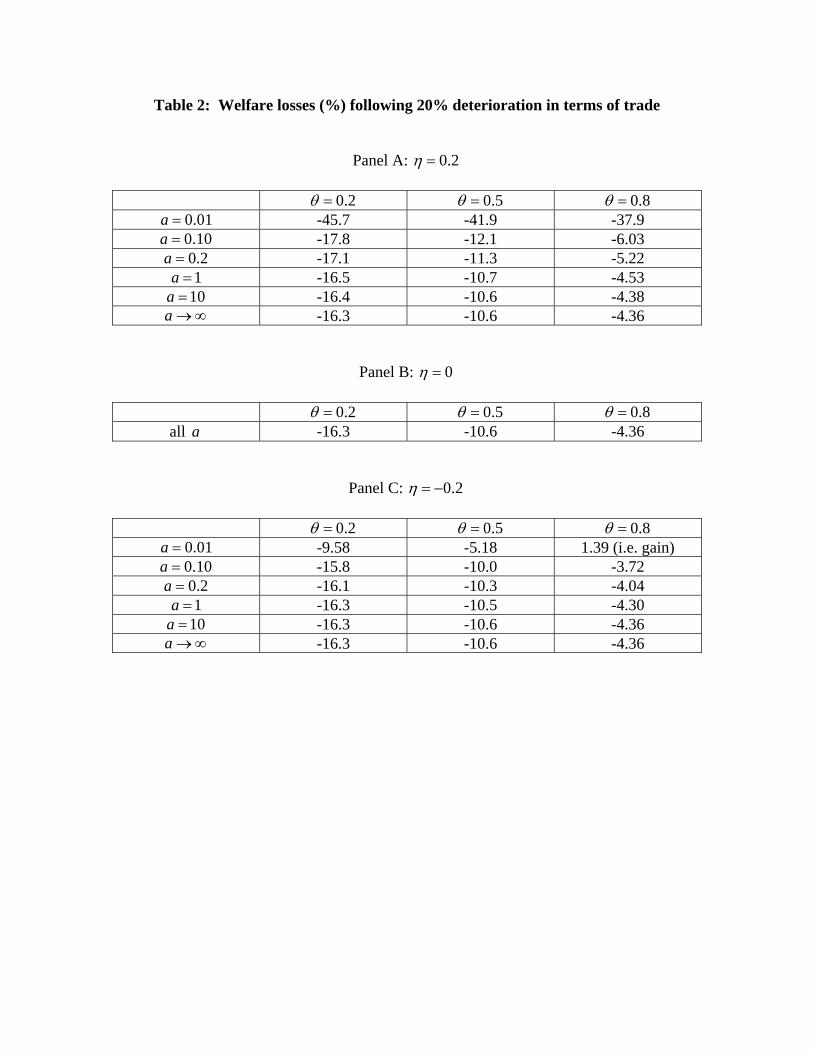
Table 2: Welfare losses (%) following 20% deterioration in terms of trade

Panel A: 0.2η =

0.2θ = 0.5θ = 0.8θ = 0.01a = -45.7 -41.9 -37.9 0.10a = -17.8 -12.1 -6.03 0.2a = -17.1 -11.3 -5.22 1a = -16.5 -10.7 -4.53

10a = -16.4 -10.6 -4.38 a →∞ -16.3 -10.6 -4.36

Panel B: 0η =

0.2θ = 0.5θ = 0.8θ = all a -16.3 -10.6 -4.36

Panel C: 0.2η = −

0.2θ = 0.5θ = 0.8θ = 0.01a = -9.58 -5.18 1.39 (i.e. gain) 0.10a = -15.8 -10.0 -3.72 0.2a = -16.1 -10.3 -4.04 1a = -16.3 -10.5 -4.30

10a = -16.3 -10.6 -4.36 a →∞ -16.3 -10.6 -4.36

50 100 150 200t

337.5

338.5

339

339.5

340

340.5

cap

337.5 338 338.5 339 339.5 340 340.5 341cap

34

36

38

40

42debt

10 20 30 40 50t

0.085

0.086

0.087

0.088

0.089

0.091

0.092borr .rate

20 40 60 80 100t

66.2

66.4

66.6

66.8

67.2

cons

20 40 60 80 100t

0.8775

0.8825

0.885

0.8875

0.89

0.8925

welfare

20 40 60 80 100t

34

36

38

40

42debt

Fig 1:Adjustments following 20% deterioration in terms of trade:Positive production externality

a. Dynamics of capital stock

b. Dynamics of debt

d. Dynamics of borrowing rate

c. Phase diagram

e. Dynamics of consumption

f. Dynamics of welfare

50 100 150 200 250 300t

45.65

45.7

45.75

45.8

45.85

cap

10 20 30 40 50t

-2.7

-2.6

-2.5

-2.4

-2.3debt

45.55 45.65 45.7 45.75 45.8 45.85cap

-2.7

-2.6

-2.5

-2.4

-2.3

-2.2

-2.1debt

10 20 30 40 50t

0.0445

0.0455

0.046

0.0465

0.047

0.0475borr .rate

20 40 60 80 100t

4.63

4.64

4.65

4.66

cons

20 40 60 80 100t

0.896

0.898

0.902

0.904

welfare

Fig 2: Adjustment following 20% deterioriation in terms of trade:Negative production externality

a. Dynamics of capital stock d. Dynamics of borrowing rate

c. Dynamics of debt

c. Phase diagram

e. Dynamics of consumption

f. Dynamics of welfare

23

References

Auerbach, A. and L. Kotlikoff, 1987, Dynamic Fiscal Policy, Cambridge University Press, New York.

Bardhan, P.K., 1967, “Optimum foreign borrowing,” in K. Shell (ed.), Essays on the Theory of Optimal Economic Growth, MIT Press, Cambridge, MA.

Barro R. J., 1996, Determinants of Economic Growth: A Cross-Country Empirical Study. NBER Working Paper 5698.

Barro, R.J. and X. Sala-i-Martin, 1992, “Public finance in models of economic growth,” Review of Economic Studies 59, 645-661.

Barro, R.J., and X. Sala-i-Martin, 1995, Economic Growth, McGraw-Hill, New York.

Bean C. R., 1986, “The terms of trade, labour supply and the current account,” Economic Journal Supplement 96, 38-46.

Bhandari, J.S., Haque, N.U., and Turnovsky, S.J., 1990, “Growth, external debt, and sovereign risk in a small open economy,” IMF Staff Papers 37, 388-417.

Botman, D., D. Dasgupta, and D. Ratha, 1999, “Determinants of Short-Term Debt and its Pro-cyclical Response to Economic Shocks,” World Bank, World Development Report Background paper.

Broda C., 2004, “Terms of trade and exchange rate regimes in developing countries,” Journal of International Economics 63, 31-58.

Broda C. and C. Tille, 2003, “Coping with terms-of-trade shocks in developing countries” Current Issues in Economics and Finance 9, Federal Reserve Bank of New York.

Caballero R. J. and S. Panageas, 2003, “Hedging Sudden Stops and Precautionary Recessions: A Quantitative Framework,” NBER Working Paper 9778.

Calvo G. A., A. Izquierdo, and L. Mejia, 2004, “On the Empirics of Sudden Stops: The Relevance of Balance-Sheet Effects,” NBER Working Paper 10520.

Chatterjee, S., G. Sakoulis and S.J. Turnovsky, 2003, “Unilateral capital transfers, public investment, and economic growth,” European Economic Review 47, 1077-1103.

Cooper, R.N. and J. Sachs, 1985, “Borrowing abroad: The debtor's perspective,” in G.W. Smith and J. T. Cuddington (eds.), International Debt and Developing Countries, World Bank, Washington, DC.

Cuadra, G. and H. Sapriza, 2006, “Sovereign Default, Terms of Trade and Interest Rates in Emerging Markets,” Banco de México Working Paper 2006-01.

Dadush, U., D. Dasgupta, and D. Ratha, 2000, “The role of short-term debt in recent crises,” Finance and Development 37, Number 4, IMF, Washington, DC.

Díaz-Alejandro, C. F., 1983, “Stories of the 1930s for the 1980s.” in P. Aspe-Armella, R.

24

Dornbusch, and M. Obstfeld (eds.), Financial Policies and the World Capital Market: The Problem of Latin American Countries, University of Chicago Press, Chicago.

Díaz-Alejandro, C. F., 1984, “Latin American debt: I don’t think we are in Kansas anymore.” Brookings Papers on Economic Activity 2, 335-403.

Duncan, R. 2003, “The Harberger-Laursen-Metzler Effect Revisited: An Indirect-Utility-Function Approach," Working Paper 250, Central Bank of Chile.

Easterly, W.E., R.Islam, and J.E. Stiglitz, 1999, “Shaken and Stirred: Volatility and Macroeconomic Paradigms for Rich and Poor Countries,” Michael Bruno Memorial Lecture presented at the XII World Congress of the International Economic Association, Buenos Aires, August 27.

Eaton, J. and M. Gersovitz, 1981, “Debt with potential repudiation: Theoretical and empirical analysis,” Review of Economic Studies 48, 289-309.

Edwards, S., 1984, “LDC foreign borrowing and default risk: An empirical investigation 1976-80,” American Economic Review 74, 726-734.

Eicher T. S. and S. J. Turnovsky, 1999a, “International capital markets and non-scale growth,” Review of International Economics 7, 171-188.

Eicher T. S. and S. J. Turnovsky, 1999b, “Non-scale models of economic growth,” Economic Journal 109, 394 – 415.

Harberger A. C., 1950, “Currency depreciation, income, and the balance of trade,” Journal of Political Economy 58, 47 – 60.

Hayashi, F. 1982, “Tobin's marginal q, average q: A neoclassical interpretation,” Econometrica 50, 213-224.

Huang, K. X. D. and Q. Meng, 2004, “The Harberger-Laursen-Metzler effect under capital market imperfections,” unpublished manuscript.

Ikeda S., 2001, “Weakly non-separable preferences and the Harberger-Laursen-Metzler effect,” Canadian Journal of Economics 34, 290-307

Jones, C., 1995a, “R&D based models of economic growth,” Journal of Political Economy 103, 759-784.

Jones, C., 1995b, “Time series tests of endogenous growth models,” Quarterly Journal of Economics 110, 495-527.

Kaminsky G. L., C. M. Reinhart, and C: A. Végh, 2003, “When It Rains, It Pours: Procyclical Capital Flows and Policies,” Mimeograph

Kose M. A., 2002, “Explaining business cycles in small open economies: How much do world prices matter?” Journal of International Economics 56, 299-327.

Laursen S. and L.A. Metzler, 1950, “Flexible exchange rates and the theory of employment,” Review of Economics and Statistics 32, 281 – 299.

25

Mansoorian A., 1993, “Habit persistence and the Harberger-Laursen-Metzler effect in an infinite horizon model,” Journal of International Economics 34, 153 – 166.

Mendosa E. G., 1995, “The terms of trade, the real exchange rate, and economic fluctuations,” International Economic Review 36,. 101-137.

Min, H. G., “Determinants of Emerging Markets Bond Spreads- Do Economic Fundamentals Matter?” Policy Research Paper No. 1988, The World Bank.

Min, H., D. Lee, C. Nam and M. Park, 2003, “Determinants of emerging market bond spreads: Cross-country evidence,” Global Finance Journal 14, 217-286.

Obstfeld M., 1982, “Aggregate spending and the terms of trade: Is there a Laursen-Metzler effect?” Quarterly Journal of Economics 97, 251-270.

Ortigueira, S., Santos, M.S., 1997. “On the speed of convergence in endogenous growth models,” American Economic Review 87, 383-399.

Otto, G., 2003, “Terms of trade shocks and the balance of trade: there is a Harberger-Laursen-Metzler effect,” Journal of International Money and Finance 22, 155-184.

Persson T. and L. E. O. Svensson, 1985, “Current account dynamics and the terms of trade: Harberger-Laursen-Metzler two generations later,” Journal of Political Economy 93, 43-65.

Peter, M., 2002, “Estimating Default Probabilities of Emerging Market Sovereigns: A New Look at a Not-So-New Literature,” University of Geneva Working Paper No: 06/2002.

Ploeg, F. van der, 1996, “Budgetary policies, foreign indebtedness, the stock market, and economic growth,” Oxford Economic Papers 48, 382-396.

Romer, P.M., 1986, “Increasing returns and long-run growth,” Journal of Political Economy 94, 1002-38.

Sen P. and S. J. Turnovsky, 1989, “Deterioration of the terms of trade and capital accumulation: A re-examination of the Laursen-Metzler effect,” Journal of International Economics 26, 227-250.

Serven, L., 1999, “Terms-of-trade shocks and optimal investment: Another look at the Laursen-Metzler effect,” Journal of International Money and Finance 18, 337-365.

Svensson L. E. O. and A. Razin, 1983, “The terms of trade and the current account: The Harberger-Laursen-Metzler effect,” Journal of Political Economy 91, 97-125.

Turnovsky, S.J., 1993, “The impact of terms of trade shocks on a small open economy: a stochastic analysis,” Journal of International Money and Finance 12, 278-297.

Turnovsky, S.J., 1996, “Fiscal policy, growth, and macroeconomic performance in a small open economy,” Journal of International Economics 40, 41-66.

Turnovsky S. J. and P. Chattopadhyay, 2003, “Volatility and growth in developing economies: some numerical results and empirical evidence,” Journal of International Economics 59, 267-295.

26

World Bank: 1993, Boom, Crisis and Adjustment, The Macroeconomic Experience of Developing Countries, Oxford University Press, Oxford.