Dynamic control of sensor networks with inferential

ecosystem modelsJim Clark, Environm, Biol, StatPankaj Agarwal, Comp SciDavid Bell, EnvironmentCarla Ellis, Comp SciPaul Flikkema, EE, NAUAlan Gelfand, Stat

Gabriel Katul, EnvironmentKamesh Munagala, Comp SciGavino Puggioni, Comp SciAdam Silberstein, Comp SciJun Yang, Comp Sci

Motivation

• Understanding forest response to global change (climate, CO2)

• Forces at many scales– Complex interactions– lagged responses

• Uneven data needs: occasionally dense, at different scales

• Wireless networks can provide dense data, across landscapes

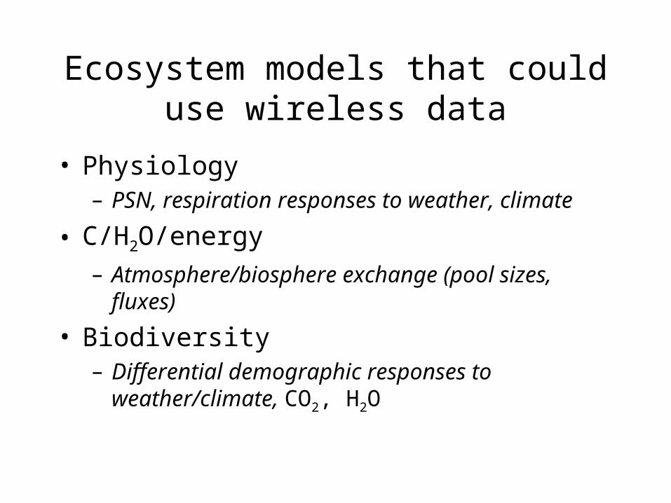
Ecosystem models that could use wireless data

• Physiology – PSN, respiration responses to weather,

climate

• C/H2O/energy– Atmosphere/biosphere exchange (pool

sizes, fluxes)

• Biodiversity– Differential demographic responses to

weather/climate, CO2, H2O

Physiological responses to weather

H2O, N, P

H2O, CO2light, CO2

Temp

PSN Resp

Sap flux

Allocation

Fast, fine scales

Precip

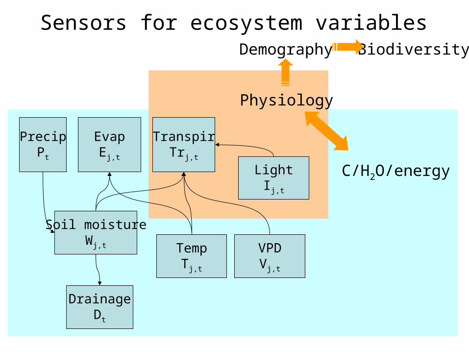
Sensors for ecosystem variables

Soil moistureWj,t

PrecipPt

EvapEj,t

TranspirTrj,t

DrainageDt

LightIj,t

TempTj,t

VPDVj,t

C/H2O/energy

Demography Biodiversity

Physiology

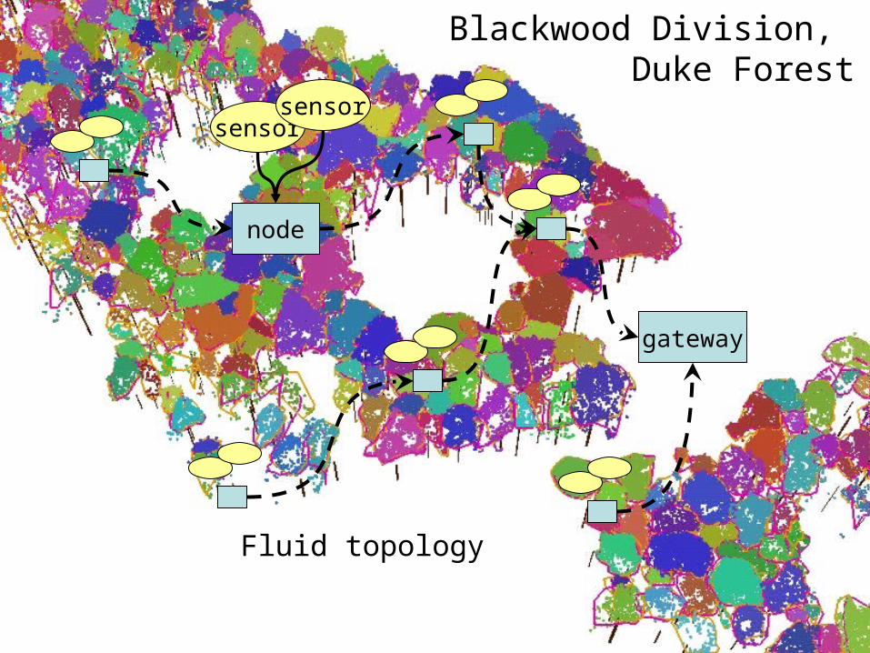
WisardNet: a wireless network

• Multihop, self-organizing– Sensors for light, soil & air T, soil moisture,

sap flux– Tower weather station

• Minimal in-network processing

node

sensorsensor

gateway

Self-organizing wireless connections

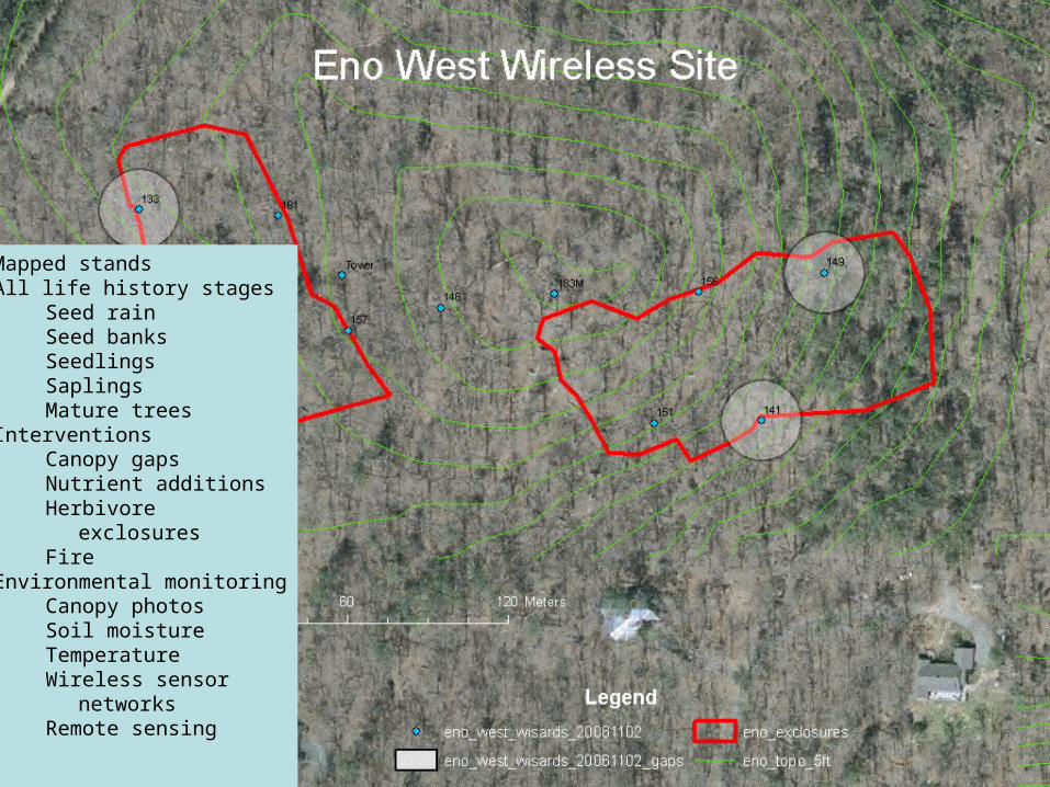
Mapped standsAll life history stages

Seed rainSeed banksSeedlingsSaplingsMature trees

InterventionsCanopy gapsNutrient additionsHerbivore exclosuresFire

Environmental monitoringCanopy photosSoil moistureTemperatureWireless sensor

networksRemote sensing

node

sensorsensor

gateway

Fluid topology

Blackwood Division, Duke Forest

The goods and the bads

•The good:-Potential to collect dense data-Adapts to changing communication potential

•The bad: -Most data uninformative, redundant, or both-Battery life of weeks to months, depending on transmission rate-Checking and replacing batteries is the primary maintenance cost of network

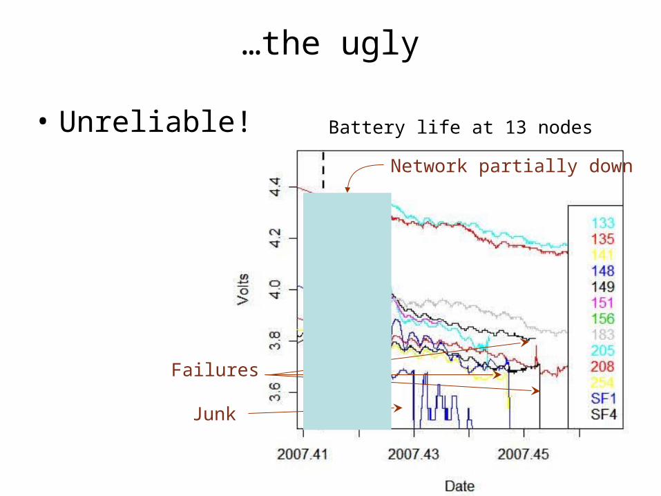
…the ugly

• Unreliable! Battery life at 13 nodes

Network partially down

Failures

Junk

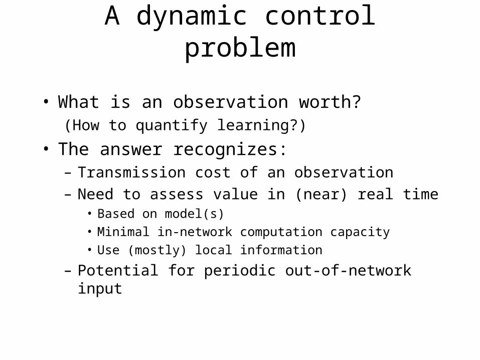
A dynamic control problem

• What is an observation worth?(How to quantify learning?)

• The answer recognizes:– Transmission cost of an observation– Need to assess value in (near) real time

• Based on model(s)• Minimal in-network computation capacity• Use (mostly) local information

– Potential for periodic out-of-network input

A framework for data collection

• ‘Predict or collect’: – Transmit an observation if it could not

have been predicted by a model.

• Fast decisions (real-time)• Must rely on (mostly) local

information– Minimize transmission

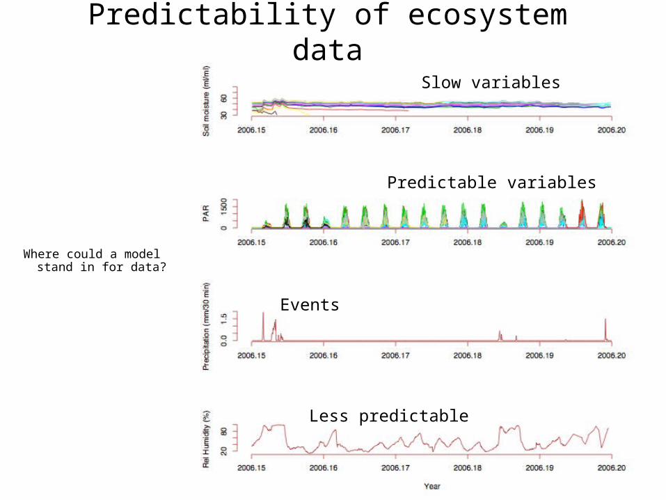
Predictability of ecosystem data

Where could a model stand in for data?

Slow variables

Predictable variables

Events

Less predictable

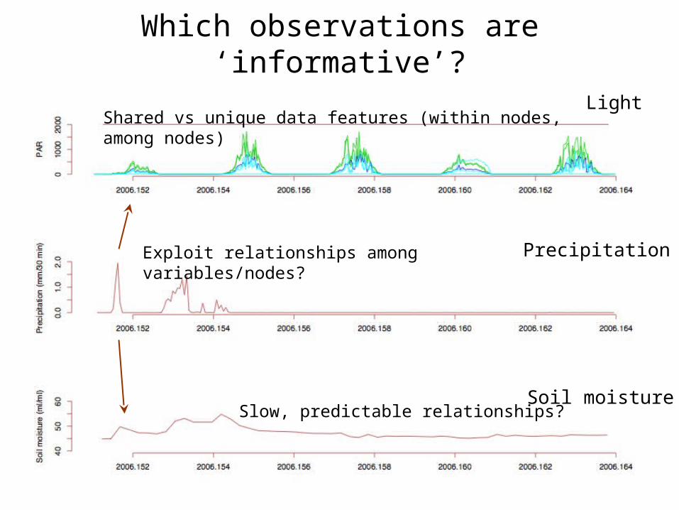
Which observations are ‘informative’?

Shared vs unique data features (within nodes, among nodes)

Exploit relationships among variables/nodes?

Slow, predictable relationships?

Light

Precipitation

Soil moisture

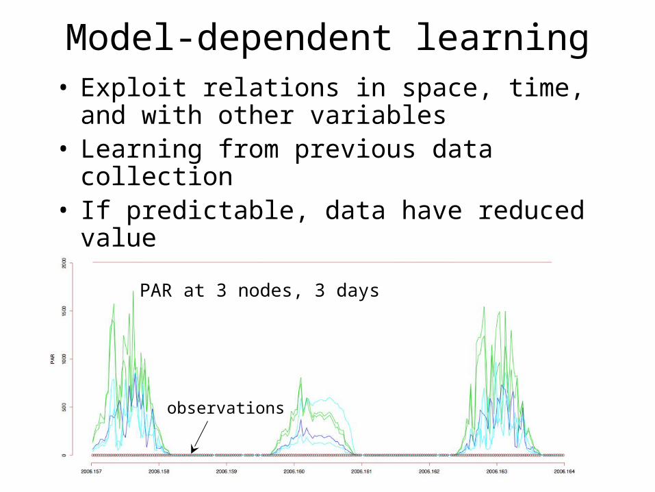
Model-dependent learning• Exploit relations in space, time, and

with other variables• Learning from previous data collection• If predictable, data have reduced value

PAR at 3 nodes, 3 days

observations

Controlling measurement with models

• Inferential modeling concerns– Some parameters ‘local’, some ‘global’ – Estimates of global parameters need

transmission– Data can’t arrive faster than model converges

• Simple rules for local control of transmission– Rely mostly on local variables– Periodic updating from out of network– ‘Transmit if you can’t predict’

In network data suppression

• An ‘acceptable error’, • A standard reactive model based on

change,

• Alternative: is the observation ‘predictable’,

€

zj,t −zj,t−1 <

€

zj,t − ′ zj,t{z} j ,{ ′ θ , ′ z MF ,z,w}t, M I <

{z}j local sensor data (no transmission){θ, z, w}t global data, periodically updated from full modelMF full, out-of-network modelMI simplified, in-network model

{y,E,Tr,D}t

Data

Calibration data (sparse!)

Process

Parameters

Hyperparameters

heterogeneity

Processparameters

€

wj,t

Location effects

time effectt-1

time effectt

time effectt+1 Measurement

errorsProcess

error

{y,E,Tr,D}t-1 {y,E,Tr,D}t+1

Out-of-network model is complex

Sensor data

zj,t

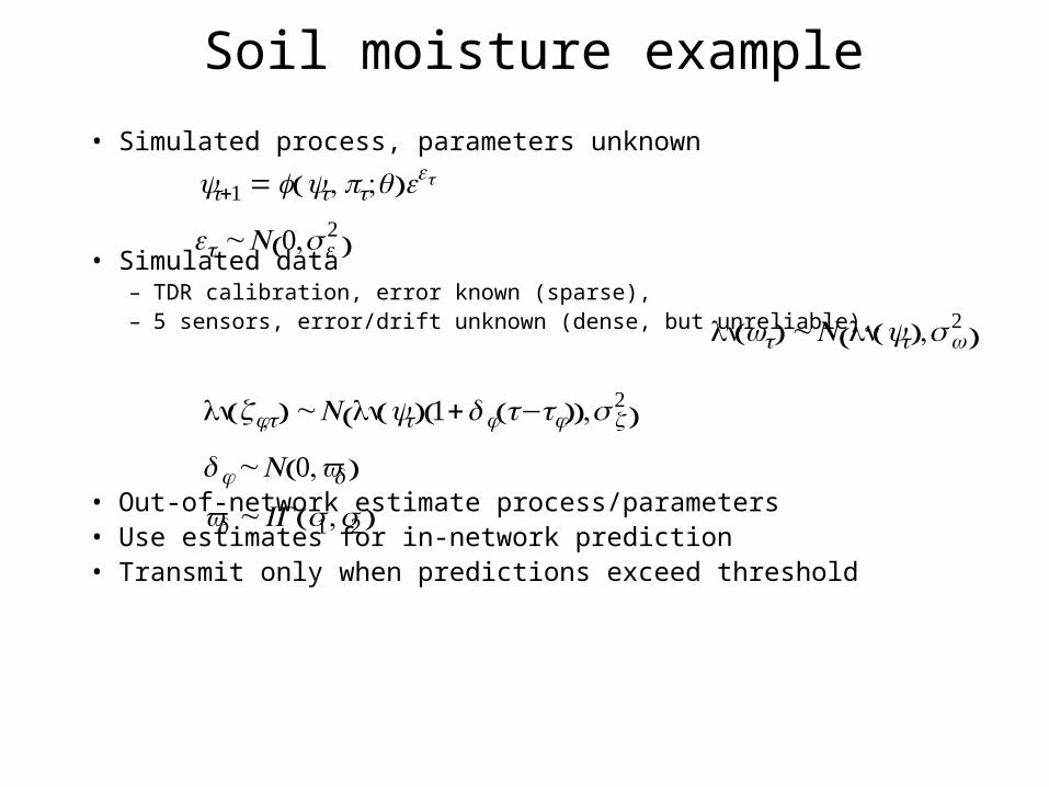
Soil moisture example

• Simulated process, parameters unknown

• Simulated data– TDR calibration, error known (sparse), – 5 sensors, error/drift unknown (dense, but unreliable),

• Out-of-network estimate process/parameters• Use estimates for in-network prediction• Transmit only when predictions exceed threshold

€

yt+1 = f yt, pt;θ( )et

t ~N 0,σ2

( )

€

ln wt( ) ~N ln yt( ),σw2

( )

€

ln zj,t( ) ~N ln yt( ) 1+δ j t−tj( )( ),σ z2

( )

δ j ~N 0,vδ( )

vδ ~IG s1,s2( )

Model summary

€

yt+1 = f yt , pt ;θ( )eεt

f yt , pt ;θ( ) = yt + pt − ET yt ;θ1,θ2( ) − D yt ;θ3( )

εt ~ N 0,σ ε2

( )

€

ln z j,t( ) ~ N ln yt( ) 1+δ j t − t j( )( ),σ z2

( )

δ j ~ N 0,vδ( )

vδ ~ IG s1,s2( )

ln wt( ) ~ N ln yt( ),σ w2

( )

Process:

Sensor j:Rand eff:

TDR calibration:

€

p y{ },θ, δ{ },σ2 ,σ z

2 z{ }, w{ }, p{ },σw2

( )Inference:

Back to node j:

€

′ θ , ′ δ j

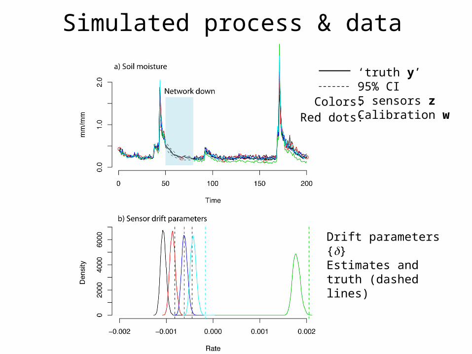
‘truth y’95% CI5 sensors zCalibration w

Colors:

Drift parameters {δ}Estimates and truth (dashed lines)

Red dots:

Simulated process & data

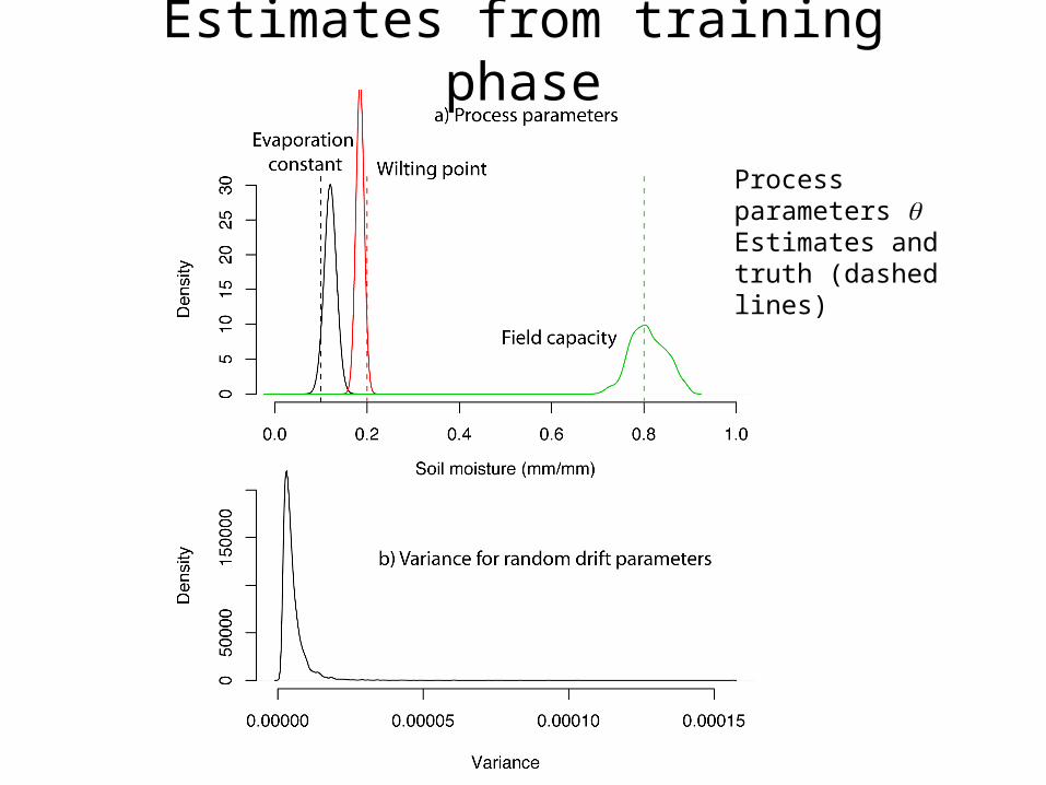
Process parameters θEstimates and truth (dashed lines)

Estimates from training phase

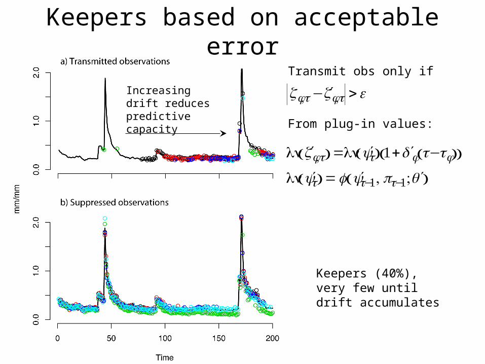
Keepers (40%), very few until drift accumulates

Increasing drift reduces predictive capacity

Keepers based on acceptable error

€

ln ′ zj,t( ) =ln ′ yt( ) 1+ ′ δ j t−t j( )( )

ln ′ yt( ) = f ′ yt−1, pt−1; ′ θ ( )

Transmit obs only if

€

zj,t − ′ zj,t >

From plug-in values:

Better ‘data’, few ‘observations’

‘truth y’95% CI5 sensors zCalibration w

Colors:Red dots:

€

p ln zj,t( ) yt, ′ zj,t,,...( )∝ N ln yt( ) 1+δ j t−tj( )( ),σ z2

( ) I ′ zj,t −( ) < zt < ′ zj,t +( )( )

Reanalysis model for missing data:

€

ln ′ zj,t( ) =ln ′ yt( ) 1+ ′ δ j t−tj( )( )

ln ′ yt( ) = f ′ yt−1, pt−1; ′ θ ( )

Known constraint on missing data

Additional variables

‘Collect or predict’

• Inferential ecosystem models: a currency for learning assessment

• In-network simplicity: point predictions based on local info, periodic out-of-network inputs

• Out-of-network predictive distributions for all variables (‘reanalysis’ step)

• A role for inference in data collection, not just data analysis

Advantages over ‘reactive’ data collection in wireless networks

• ‘Change’ in a variable is not directly linked to its information content– Example: all soil moisture sensors may

change at similar rates, making them largely redundant

• ‘Predictability’ emphasizes change that contains information

• The capacity to predict an observation summarizes its value and assures that it can be estimated to known precision in the reanalysis