Dynamic Content Variation with Customer Learning

Fernando Bernstein, Soudipta Chakraborty, and Robert Swinney∗

August, 2020

Abstract

Problem Definition: We analyze a firm that sells repeatedly to a customer populationover multiple periods. While this setting has been studied extensively in the context of dynamicpricing—selling the same product in each period at a dynamically varying price—we considera different approach: dynamic content variation wherein the product is sold at the same pricein every period, but the firm may vary the content of its product over time. Customers learnabout their utility on purchasing and decide whether to repeat a purchase in each future period.The firm faces a budget for the total value of content it can use over a finite planning horizon,and decides how to allocate this budget to each period to maximize revenue.Academic/Practical Relevance: A number of new business models, such as video streamingservices and curated subscription boxes, face the situation that we model. Our results show howsuch firms can optimally use dynamic content variation to increase their revenues.Methodology: We use an analytical model in which rational customers decide whether topurchase in a period and a firm determines an optimal content allocation policy to maximizerevenue.Results: The firm’s optimal allocation policy is not, in general, constant over time, but ismonotone. Specifically, content value should increase during a planning horizon if customerheterogeneity is low and decrease otherwise. Across successive planning horizons, content valueis cyclical with periods of high and low value, but unless the market growth rate is consistentlyhigh (e.g., exponential), content value will converge to a constant and equal allocation in everyperiod as more customers learn their utility.Managerial Implications: We show how firms can dynamically vary content to increaserevenues. Thus, managers at such firms may engage in dynamic content variation, instead ofdynamic pricing, as a revenue management strategy.

Keywords: dynamic content variation; revenue management; customer learning

1 Introduction

In recent years, a number of successful new business models, primarily services, have arisen that

incorporate the following combination of features:

1. Customers purchase (or experience service) from the firm repeatedly over successive periods.

2. The firm charges a fixed price for each purchase or service experience across all periods.

3. While the firm does not change the price from one period to the next, it can change the

content that it offers to customers in each period.

∗Bernstein and Swinney: Duke University, {fernando.bernstein@duke.edu, robert.swinney@duke.edu}.Chakraborty: University of Kansas, soudipta.c@ku.edu.

1

Two prominent examples are video streaming services and curated subscription boxes. Video

streaming services such as Netflix, Apple TV+, Hulu, and Disney+ provide customers access to a

catalog of content (typically films or television series, produced both in-house and by third party

production companies) for a monthly subscription fee. While the subscription fee is pre-determined

and seldom changes (Forbes 2019), the catalog is regularly updated by adding new content, i.e.,

by producing new movies and series or purchasing the broadcast rights to third-party content,

and by removing older content (Engadget 2018, Digital Trends 2020). Thus, customers purchase

repeatedly (they subscribe on a monthly basis, typically without an obligation to commit more

than one month at a time) at a fixed price for each purchase, but the content offered (the video on

the streaming service) changes on a continual basis.

Similarly, curation subscription box services ship unique collections of related physical goods

to customers at regular intervals, e.g., weekly or monthly, for a fixed, pre-determined, per-box

price. Examples of the types of items offered via this business model include meal kits (Blue Apron

and Hello Fresh), cosmetics and personal care items (Birchbox and Ipsy), and even pet products

(BarkBox). As with streaming video services, subscription box customers repeatedly purchase at

a fixed price per box received, while the firm may vary the box contents offered in each period.

The features illustrated in these examples stand in contrast to many traditional business models

that involve selling a fixed set of products over multiple periods, but at a price that changes from one

period to the next. This allows traditional firms to engage in dynamic pricing, i.e., to manipulate

the price over time to maximize revenue, a practice that has received enormous research attention

in the last two decades (Talluri & Van Ryzin 2006). The service providers in our examples, however,

generally do not engage in dynamic pricing: rather, video streaming and subscription box services

have a different lever at their disposal, as they can allocate content over time to influence customer

purchasing decisions. We refer to this resource allocation problem as dynamic content variation,

and this practice is precisely what we study as we seek to understand how firms can optimally vary

the content they offer over time—rather than price—in order to maximize revenue.

To accomplish this, we analyze a stylized model of a service provider determining content over

multiple successive periods in a finite planning horizon. In each period, customers decide whether

to purchase based on the current content that is offered by the provider—e.g., the current set of

movies or TV series available on Netflix, or the current set of menu items on a meal kit service like

2

Blue Apron. A key element of the businesses in these examples is that their customers experience

multiple sources of utility. First, they experience some utility from the content that they gain access

to (i.e., the particular movies or series offered on a streaming service, or the items for a curation

subscription box). This utility is typically known to customers in advance of a purchase decision:

for instance, Netflix heavily advertises new movies and series before they are released, while meal

kit services list menus on their websites for the next several weeks.

However, beyond the utility for the content they receive, customers also experience some service

utility from receiving that content. Video streaming services do not just offer movies and TV series,

they also offer a user interface that helps customers navigate and select what to watch, personalized

recommendations for new content, and a convenient way of watching video (compared to purchasing

or renting physical media). Curation subscription services do not just offer the items in the box,

they also curate those items (search for novel and interesting items to offer), package them in

a box, and deliver them to the homes of customers on a regular basis. This “service” element

of customer utility is typically not known by new customers until they experience the service at

least once—for instance, a customer does not know whether they like the Netflix user interface

and content recommendation algorithm until they use Netflix—and thus it must be learned via a

service experience. Similarly, a meal kit customer can only find out whether they like Blue Apron’s

curation and delivery service by subscribing to it.

These dual sources of utility—content utility, which the firm can manipulate over time via its

content allocation decisions, and service utility, which is constant from one period to the next but

initially unknown to new customers—play important roles in the purchasing decisions of customers

as well as the content decisions of the service provider. For example, because they do not yet

know their service utility, new customers may need to be enticed to try the service by offering

exceptional content, such as a hit TV series or a trendy new recipe. This would seem to suggest

that the service provider could benefit from placing content of significant value early in the planning

horizon, encouraging many new customers to experience the service and learn their utility. However,

if the provider allocates all of its best content early on, customers may choose not to purchase in

subsequent periods, knowing that the remaining content is less appealing. Moreover, because of

their different needs and tastes, both components of utility will, in general, be heterogeneous among

customers.

3

What makes this problem especially challenging is the fact that service providers are resource-

constrained. Put concretely: if Netflix could offer hundreds of hit new series and movies each

month, it would be able to attract many new subscribers and entice them to continue as customers

month after month. However, this would be prohibitively expensive, as the cost of a television

series can exceed $15 million per episode (for special effects heavy shows like The Mandalorian

on Disney+, but also for shows with highly paid stars like The Morning Show on Apple TV+)

while films can cost hundreds of millions of dollars. Since Netflix does not have infinite resources

to produce new content, it must operate with a budget, and allocating more resources for new

content in one month would mean less resources for others; in turn, while this would raise demand

for months with a high allocation of resources, it would result in lower customer content utility and

reduced demand in months with a lower allocation of resources.

This leads to our main research question: given the dual sources of customer utility and the

experiential nature inherent in service utility, how should a service provider allocate finite resources

over time to both attract and retain customers? To give a specific example using the case of a

streaming video provider: within a planning horizon (say, a fiscal year) should Netflix release all

its best new series and movies at once, should it spread them out equally over time, or it should it

follow some other strategy? The service provider in our model thus faces a constrained optimization

problem with an exogenously specified total budget for content over a planning horizon of T ≥ 2

discrete time periods. Customers dynamically choose in each period whether to pay the service

provider’s fee and access the content offered in that period based on their assessment of the total

utility, i.e., the sum of the content and service utility, in that period. Customers are heterogeneous

in both dimensions of utility; however, by allocating more of its content budget to a period, the

service provider can raise the average content utility in that period.

Using this framework, we determine precisely how the service provider should allocate its content

budget to the individual periods over the planning horizon to maximize revenue. Interestingly, we

find that, in general, the optimal policy does not necessarily result in an equal allocation of the

content budget in every period; however, the optimal policy generally is monotone. The critical

factors that determine whether the optimal allocation increases or decreases over time include the

degree of customer heterogeneity, the relative number of new and repeat customers, and the rate

of growth of the customer population. Our results thus show that these service providers can

4

employ dynamic content variation to influence customer purchasing decisions, manipulate the rate

of customer learning about their service utility, and increase revenue, much like more traditional

firms can dynamically vary prices from one period to the next to improve performance.

Our analysis proceeds as follows. In §2, we review the related literature. In §3, we describe

the details of our model. In §4 we derive the service provider’s optimal content allocation strategy

within a single finite planning horizon. Finally, in §5 we consider how content allocation should

change over successive planning horizons as the characteristics of the customer population evolve,

i.e., as existing customers learn about their service utility, and new customers arrive. §6 concludes

the paper.

2 Literature Review

Our work lies at the intersection of several streams of research. The first is a stream of literature

in which demand in a period is dependent on various aspects of past interactions between a firm

and its customers such as service failure (Hall & Porteus 2000), price (Popescu & Wu 2007), sales-

force effort (Liu et al. 2007), capacity (Liu & van Ryzin 2011), fill rate (Adelman & Mersereau

2013), service level (Aflaki & Popescu 2014), etc. Many of these papers assume behavioral models

such as loss aversion, goodwill formation, and habituation to link the seller’s decision and the

customers’ actions between different periods. In Caulkins et al. (2006), a firm sells a good at a

fixed pre-determined price but can manipulate its quality over time. The quality choice determines

the seller’s reputation which in turn drives future sales. Another group of paper studies how parts

of an experiential service should be optimally sequenced to maximize the total perceived utility

of a customer (Verhoef et al. 2004, Dixon & Verma 2013, Dixon & Thompson 2016, Das Gupta

et al. 2016). The perceived utility depends on various behavioral effects like decreasing impatience,

satiation, and habit formation (Wathieu 1997, Baucells & Sarin 2007, 2010). In contrast to these

papers, we do not focus on any customer behavioral aspects; instead, in our model, the value of

content in the current period affects future demand in two ways. First, it determines how much

of the budget for content is left for the remaining periods. Second, once a customer signs up and

uses the service, he learns his service utility and makes future purchasing decisions based on this

realized utility and the value of the content in future periods. Hence, the provider optimally varies

5

the content value over time to influence the rate at which it gains new customers and the rate at

which it persuades existing customers to continue using the service.

The problem of how a firm should change its assortment of products during a selling season has

also been studied (Caro et al. 2014, Bernstein & Martınez-de Albeniz 2017, Ferreira & Goh 2018).

Our paper is different than much of the assortment literature because the customers in our model

access the entire set of content and not individual products from an assortment. Somewhat closer

to our work is Caro & Martınez-de Albeniz (2020), who study how a content creator can maximize

traffic to a website by exerting costly effort over multiple periods to produce new content. However,

their model does not incorporate customer learning or an explicit model of customer purchasing

decisions, as our model does; rather, in their paper, customers arrive to the website according to a

Poisson arrival stream that is an increasing function of the content released in a particular period.

These modeling differences lead to very different results: for example, Caro & Martınez-de Albeniz

(2020) show that the optimal policy is to weakly increase content over time, whereas we show

that, depending on the degree of customer heterogeneity, it may be optimal to increase or decrease

content value over time.

Using a customer utility model that is somewhat similar to ours, Feldman et al. (2019) study

the quality decision of a firm selling a new experience good to customers who may strategically

delay a purchase to learn more information about quality. Hence, unlike Caro & Martınez-de

Albeniz (2020), they include both customer learning and an explicit model of customer purchasing

decisions, as we do; however, the situation they study is quite different from ours. For example,

we consider the optimal allocation of content across multiple periods with a fixed price, whereas

they model a one-time quality (and price) decision that is constant throughout the time horizon.

In addition, customers in our model decide whether to use the service in each period—and in

particular, customers may use the service multiple times within the horizon—while customers in

Feldman et al. (2019) buy the product at most once. Hence, while Feldman et al. (2019) do not

consider the issue of encouraging repeat purchases via the use of a dynamic content (or quality)

allocation policy, that is the focus of our paper.

To summarize, our model is the first, to our knowledge, in which a firm sells a non-durable good

that customers can repeatedly purchase at a fixed price over multiple periods, and the firm must

allocate a finite budget for the value of its product to each period in order to maximize revenue.

6

3 Model

In the following two subsections, we describe the decisions made by the two key sets of players in

our model: customers (in §3.1) and the service provider (in §3.2).

3.1 Customers

A service provider offers a set of content over a planning horizon consisting of T (≥ 2) periods.

In each period, customers can gain access to this content by paying an exogenous price p that is

constant throughout the planning horizon; as noted in the introduction, the prices for the types of

firms that motivate our model are typically long-term, strategic decisions that change infrequently

(Forbes 2018, USA Today 2019). Following our discussion in §1, each customer’s utility can be

divided into two additive parts: content utility and service utility. Customers are heterogeneous in

both components. Specifically, customer i’s content utility in period t is given by

vit = vt + εit, (1)

where vt is the mean utility derived from period t content, and εit ∼ N(0, σ2ε ) is a mean zero term

specific to customer i. We refer to vt as the value of the content, and it is this value that is chosen

by the provider when it chooses the content in each period (more on this choice will be discussed in

§3.2); hence, a higher value of vt results in higher average utility in the customer population. The

second term, εit, captures customer-specific heterogeneity in taste for the same content; higher σε

means customers have more heterogeneous tastes. At the beginning of every period, a customer

observes the content available for that period and his realized content utility vit. However, for

any customer i, εit is unobserved by the provider; hence, when choosing vt before period t, it only

relies on the distribution of εit in the customer population. Customer i’s realizations of εit are

independent across periods, which is appropriate if there is sufficient variety in the content from

one period to the next (i.e., different genres of TV series for a streaming video platform or different

types of cuisine for a meal kit service).

Customers are also heterogeneous in their service utility, θi, which is distributed over the cus-

tomer population as θi ∼ N(µ, σ2θ). This component includes all elements of customer utility

7

that do not originate from the provider’s content decisions, and thus depends on various inherent

features of the provider’s service (independent of the content) that are difficult to change in the

short-term. As a result, θi does not change from one period to the next, i.e., it does not depend

on t. Instead, it depends on how well these features match the idiosyncratic needs of a customer,

i.e., whether the customer happens to like the user interface of a streaming video provider or the

curation and delivery service of a subscription box provider. Hence, service utility differs from one

customer to the next, resulting in its distribution over the customer population and dependence

on i. Higher σθ means that customers have more heterogeneous valuations for the service. Putting

the two components—content utility and service utility—together, customer i receives total utility

(net of the purchase price) equal to

uit = θi + vt + εit − p (2)

from accessing the content of value vt in period t.

Before customers have received service from the provider, they will not know how well the

provider executes that service nor whether it fits with their expectations; hence, before signing up

and using the service for the first time, customer i will not know θi beyond its distribution over

the population. We assume that after using the service for the first time, the customer perfectly

learns his service utility, θi. Mathematically, the customer observes his realization of total utility

in period t, uit, and using (2), infers his draw of θi = uit − vt − εit + p. In all subsequent periods,

the customer will know his realized service utility θi when making his purchasing decision. Just

as in the case of the content utility, the service provider cannot observe the realization of θi for

a particular customer, and instead uses its distribution in the customer population to determine

content.

We note here that it is possible that before signing up for the service, some components of

content utility might not be known to customers (e.g., customers who have never used a service

might be aware of only the more popular or heavily advertised items in the provider’s set of contents

in a period but not aware of the less popular ones), while they might know certain aspects of their

service utility (e.g., someone who has used a competitor service before will have a general idea of

his usefulness for the overall service category). Our model also extends to such situations as we

8

can relabel the component of customer i’s total utility that he knows before signing up in period t

as vit = vt + εit and all the remaining components, either from the the content or from the service,

that are revealed only after signing up as θi. The key features in the model are that some portion of

utility (regardless of its label) is only learned by customers after using the service, and the service

provider can increase the average utility of customers (again regardless of the label) by allocating

more resources to a time period.

All customers choose, in each period, whether they wish to access the content for that period

by paying the price p or not, and they incur no hassle cost for “pausing” or “restarting” their

service. In the examples discussed in §1, providers generally make it very easy for customers to

visit their website to sign-up or pause a service, e.g., it is nearly frictionless to pause and restart a

subscription for Netflix or Hello Fresh. Although we ignore any hassle cost that a customer incurs

to start, stop, or resume service, it can be included in our model in the form of an extra subtractive

term. Customers are risk neutral with zero outside option value; hence, a customer who has never

used the service before will subscribe for the first time in period t if E[uit] = µ + vt + εit − p ≥ 0.

After receiving service at least once and observing θi, he would subscribe again in a later period

t′(> t) if uit′ = θi + vt′ + εit′ − p ≥ 0.

At the beginning of the planning horizon, the market consists of a unit mass of customers, an

α ∈ [0, 1] fraction of whom have used the service at some point in the past (i.e., before period 1)

and are aware of their utility, θi. In other words, an α fraction of the market are repeat customers

while the remaining 1 − α fraction are new customers, who have never used the service before

and need to sign up to learn θi. In §4, we suppose that the market size remains constant at 1

throughout the planning horizon and study the provider’s optimal budget allocation strategy for

this market. However, it is possible that over time additional new customers arrive and expand the

overall size of the market. This, combined with the fact that within a planning horizon even absent

new arrivals, some of the existing customers will sign up and learn θi, will change the value of α

at the beginning of the next planning horizon. We study this dynamic in §5, and consider how α

itself and the provider’s choice of content value evolve over successive planning horizons as existing

customers learn and new customers arrive.

9

3.2 Service Provider

As noted previously, the price p for the service is exogenously specified and fixed throughout the

planning horizon. Similarly, the mean customer service utility, µ, depends on various long term

decisions about the characteristics of the service (e.g., tools used for personalized recommendation,

offline download rules, number of parallel devices supported, parental controls, etc. for streaming

services; fulfillment capabilities, supplier quality, delivery partner quality, etc. for subscription

boxes), and is also exogenous and fixed for the duration of the planning horizon. This leaves

dynamic content allocation as the only remaining lever for the provider to influence customer

purchasing decisions.

Creating content often comes with a significant leadtime: in the case of streaming services, TV

series and movies can take a year or more to produce, while subscription boxes must source inventory

for their boxes weeks or months in advance. Thus, before period 1, the provider decides the contents

for the entire planning horizon of T periods. This planning horizon may be generated by financial

considerations (for instance, a fiscal year for a streaming video provider), or it may be generated

by the nature of the provider’s business (e.g., meal kit providers typically list menus for the next

4-8 weeks to give customers time to make their decisions). Because the provider does not directly

observe customer valuations, it learns no new information, nor is there any stochasticity throughout

the planning horizon (that is, only customers learn information—their individual utilities for the

service after accessing the content at least once); hence, there is no difference between the open

loop policy wherein the provider chooses content for all T periods before period 1 and a closed loop

policy that gives the provider recourse to change the content decision at the start of every period.

As noted previously, what makes this problem challenging is that the provider has finite re-

sources and cannot simply allocate very high content value in every period. To reflect this, we

introduce a budget V for the total value of content over a planning horizon of T periods. This

budget is infinitely divisible and the provider can allocate any value, vt ≥ 0 to content in period

t ∈ {1, 2, ..., T}, provided the total of the content over the T periods satisfies ΣTt=1vt ≤ V . The

provider’s objective is to maximize the total expected demand during the planning horizon; since

the per period price, p, is constant, this is equivalent to maximizing revenue. We discuss further

details of the provider’s objective function in the next section, but it is easy to see from (2) that

10

a higher value of content in a period increases the utility of customers, and consequently, the like-

lihood that they would be willing to pay the price p. Hence, the provider will always exhaust the

total budget over the time horizon. Therefore, the provider will choose the content values subject

to the budget constraint:

ΣTt=1vt = V, where vt ≥ 0 ∀ t. (3)

The simplicity of the budget constraint allows us to analyze a complicated objective function

(derived in Proposition 1) while enforcing a key trade-off: the provider cannot offer highly valuable

content that results in high demand in every period, and hence it must allocate finite resources

to balance the rate at which it persuades new customers to sign up and repeat customers to use

the service again. Since items that are higher in value to customers should also be costlier for the

provider to offer (Mussa & Rosen 1978, Desai 2001, Jerath et al. 2017), we could also assign some

cost c per unit of content value, and then require that the provider maximize revenue subject to

the constraint that total content expenditure not exceed cV , i.e., that ΣTt=1cvt = cV . Observe that

the cost c appears on both sides of this inequality; hence, we may think of the budget constraint

merely as a limit on the total value, and the budget on value plays the same role as a constraint

on the operating cost of the service.

4 Optimal Content Allocation Within a Single Planning Horizon

We now derive the optimal content allocation policy within a finite planning horizon. The provider

decides on content values v1, v2, ..., vT before period 1 to maximize total expected demand (equiv-

alently, revenue) over the planning horizon. Let φ(·), Φ(·), and Φ(·) denote the pdf, cdf, and

complementary cdf functions of the standard normal distribution, respectively. This leads to our

first result, which derives the objective function of the service provider:

11

Proposition 1. For all content values v1, v2, ..., vT set by the service provider, expected total de-

mand over the planning horizon is

E[D] =α

T∑t=1

Φ

p− µ− vt√σ2ε + σ2

θ

+ (1− α)

1−T∏t=1

Φ

(p− µ− vt

σε

)+

T∑t=2

{1−

t−1∏i=1

Φ

(p− µ− vi

σε

)}Φ

p− µ− vt√σ2ε + σ2

θ

.(4)

Proof. All proofs appear in Appendix A.

From the customer utility function (2), a new customer i will only use the service in period

t ∈ {1, 2, ..., T} if his expected utility satisfies E[uit] = µ+ vt + εit − p ≥ 0, i.e., if his idiosyncratic

taste for the content is εit ≥ p− µ− vt. From the provider’s perspective, customer i’s probability

of using the service in period t is thus Φ(p−µ−vtσε

). On using the service in period t, the customer

observes the realization of his total utility, uit, and infers θi accurately. He will then pay the price

p to use the service again in period t′ ∈ {t+ 1, ..., T} if uit′ = θi + vt′ + εit′ − p ≥ 0. The provider

neither knows θi nor εit′ ; hence, for the provider, uit′ ∼ N(µ+ vt′ − p, σ2ε + σ2

θ). The provider thus

calculates that customer i will use the service again in period t′

with probability Φ

(p−µ−v

t′√

σ2ε+σ2

θ

).

On the other hand, a repeat customer j, who has used the service in a previous planning horizon,

knows his utility θj in period 1. Therefore, he will use the service in period t ∈ {1, 2, ..., T}, if

ujt = θj + vt + εjt − p ≥ 0. By the same argument, ujt ∼ N(µ + vt − p, σ2ε + σ2

θ) for the provider

and it calculates that customer j would use the service in period t with probability Φ

(p−µ−vt√σ2ε+σ2

θ

).

The expected demand function (4) has a very intuitive form. The first term, α∑T

t=1 Φ

(p−µ−vt√σ2ε+σ2

θ

),

is the expected demand from customers who were signed up before period 1. Since, these customers

do not need to learn θi by signing up, their purchasing behavior, and consequently, the form of their

demand functions will be identical in all periods. The second term captures the expected demand

of customers who are new at the beginning of the planning horizon. The term 1−∏Tt=1 Φ

(p−µ−vtσε

)is the probability that a new customer uses the service at least once during the T periods. Hence,

this is the total mass of these initially new customers who sign up and learn their utility, θi during

12

the planning horizon. The term Φ

(p−µ−vt√σ2ε+σ2

θ

)[1−

∏t−1i=1 Φ

(p−µ−viσε

)]is the probability that a new

customer who has signed up between periods 1 to t−1 uses the service again in period t ∈ {2, ..., T}.

The provider needs to maximize its expected demand (4), subject to the budget constraint (3).

The standard deviation of θi, σθ, plays an important role for both the provider and for customers.

If σθ > 0, customers are heterogeneous in their utility from the value provided by the service, and

new customers are unaware of their total utility before period 1 and need to use the service to learn

it. To study the effect of this parameter on the provider’s optimal content allocation, let us begin

with the benchmark case of σθ = 0. In this case, the entire customer population has the same

utility, µ, from service and they all know this parameter accurately; as a result, customers only

differ in their idiosyncratic preference for content, εit. This extreme case has a particularly simple

optimal value allocation that serves as a useful benchmark for our subsequent analysis.

Proposition 2. When customers have a known, homogeneous utility for service, i.e., σθ = 0, then

there exists a threshold V ≥ T (p− µ) such that for any V > V , v∗t = V/T ∀ t ∈ {1, 2, ..., T} is the

unique optimal value allocation.

When σθ = 0, the expected demand function, (4), simplifies to E[D] =∑T

t=1 Φ(p−µ−vtσε

). In

the absence of any learning by new customers, the content values among the T periods are only

connected through the budget constraint. Moreover, if the provider swaps the contents between

any two periods of the planning horizon, its expected demand will not change. Expected demand

increases as the provider increases the value of its content in any period; however, the rate of

increase is not uniform because of the “S”-shape of the standard normal cdf function that is convex

and increasing for all negative arguments and concave and increasing for all positive arguments.

The “S”-shape results in decreasing returns to scale at the extremes—very small values of vt, as

well as very large values of vt—and increasing returns to scale for intermediate values of vt.

The combination of exchangeability of content value between periods and decreasing returns to

scale at high value levels together imply that for a sufficiently high content budget, the optimal

strategy is equal allocation across periods: allocating more content to one period than another

means the period with lower content value has a higher marginal return to additional value than

the period with higher content value, and the provider is better off equalizing value in the two

periods. Hence, when the provider’s budget is higher than a threshold, it finds it optimal to divide

13

its budget equally among all periods, i.e., v∗t = V/T for any t ∈ {1, 2, ...T}.

This is only optimal, however, if the budget is high enough such that dividing it equally allocates

sufficient value in each period resulting in decreasing returns to scale for all vt. For smaller budgets,

an equal division would cause decreasing returns to scale in all periods because of low values of vt.

As a result, the provider will find it optimal to concentrate its budget among a subset of the T

periods while offering very low content value in the rest of the periods. Even though the provider

will attract very few customers in the periods with low value, aggregate expected demand will still

be higher than if it allocated the budget equally in all T periods. In the proof of Proposition 2, we

show that when V ≤ V , dividing the budget equally among some of the T periods and offering 0

value in the rest maximizes the expected demand, resulting in multiple optimal allocations.

For the remainder of the analysis, we focus on the case V > V , for two reasons. First, there

is always a unique optimal allocation. Second, under this condition, any variation in value during

the planning horizon will only arise because of a positive σθ, per Proposition 2, allowing us to

isolate the effect of customer learning about the value of the service, θi. In line with Proposition

2, we numerically observe that when V ≤ V and σθ > 0, the provider sets disproportionately high

content values towards the beginning of the planning horizon to take advantage of the increasing

returns to scale. Hence, even for positive σθ, the optimal allocation policy is primarily driven by

budget scarcity. In what follows, we focus instead on the more interesting case of a budget that

is high enough to permit a variety of content allocation strategies, and the choice between them is

non-trivial.

We now return to the case where the customer service utility is heterogeneous, i.e., σθ > 0, and

as a result customers must learn this value by using the service at least once. From (2), if customer

i knew θi before period 1, then from the provider’s perspective, uit ∼ N(µ+ v−p, σ2ε +σ2

θ). Hence,

expected demand would be

E[D] =

T∑t=1

Φ

p− µ− vt√σ2ε + σ2

θ

. (5)

From the expected demand function, (4), (5) represents the expected demand from the repeat

customer segment. By using the same logic as in Proposition 2, we can conclude that if the market

only consists of repeat customers (i.e., α = 1), the provider should allocate a value V/T to all

periods for any V > V . On the other hand, when α < 1 and there are new customers in the

14

market, offering content of equal value in every period is not necessarily optimal. This is because

the new customers’ purchasing behavior changes once they have used the service and learned θi.

By varying content value, the provider can affect the rates at which new customers who have never

used the service before purchase, and repeat customers—including new customers who experienced

service earlier in the planning horizon and learned θi—use the service again.

We now proceed to derive the optimal content allocation policy when σθ > 0, dividing our

analysis into three parts: small σθ, large σθ, and intermediate σθ. First, suppose σθ is small, but

still non-zero, i.e., σθ → 0. Then we have the following result:

Proposition 3. Let xc ≈ −0.84 be the unique solution to Φ(x) − x2Φ(x) + xφ(x) = 0. When

σθ → 0:

(i) For a high content budget, V > max{V , T (p− µ− xcσε)

}, the service provider should weakly

increase the value of content over time, i.e., set v∗t ≤ v∗t′ for any 1 ≤ t < t′ ≤ T .

(ii) For a moderate content budget, V ∈(V , T (p− µ− xcσε)

), the service provider should weakly

decrease the value of content over time, i.e., set v∗t ≥ v∗t′ for any 1 ≤ t < t′ ≤ T .

From (4), the total mass of new customers gained over the planning horizon, 1−∏Tt=1 Φ

(p−µ−vtσε

),

is independent of the order of content values, and will remain unchanged if the provider swaps the

values between two periods, t and t′. However, the order of content values is important in determin-

ing repeat usages—the fraction of new customers signing up in period t who use the service again

before the end of the planning horizon. Because of this, as the proposition shows, when σθ is small

(but positive), not only is the optimal allocation policy not constant over time, it is monotonic,

and can be either increasing or decreasing.

To understand this result, note that from (4), the total number of repeat purchases in period t

from new customers gained earlier in the planning horizon is the product of two terms:

[1−

t−1∏i=1

Φ

(p− µ− vi

σε

)]Φ

p− µ− vt√σ2ε + σ2

θ

. (6)

The first term is the number of initial purchases by new customers in periods prior to t, while

the second is the fraction of those customers who have net positive total utility given vt and their

observed θi. This product plays a key role in determining the service provider’s optimal allocation

15

policy: a decreasing value allocation over time prioritizes the first term (i.e., there are more initial

purchases), while an increasing value allocation over time prioritizes the second term (i.e., there

are fewer initial, but more repeat, purchases). Which of these is optimal depends on the total size

of the content budget, V .

If the budget is high(V > max

{V , T (p− µ− xcσε)

}), an increasing allocation maximizes de-

mand: in this case, there is sufficient budget to both start with a high content value level (leading

to a large number of initial purchases, i.e., a large value for the first term of (6)) and to induce

an increasing number of repeat purchases over time with progressively higher content value (the

second term of (6)). On the other hand, if the budget is moderate(V ∈

(V , T (p− µ− xcσε)

)), an

increasing allocation would necessitate starting with a content value that is too low (leading to few

initial purchases, i.e., making the first term of (6) very small, and hence lowering the number of

possible repeat purchases); the provider would be better off starting with a high content value and

decreasing it over time, thereby increasing the number of customers who experience the service at

least once.

This result shows that dynamic content variation (i.e., deviating from a constant value policy)

can be optimal for the provider, and moreover, the optimal policy is monotonic over time. However,

varying the value of content over time comes at a cost: demand from the repeat customer segment

who signed up before period 1. Since these customers already know their utility, they are less likely

to use the service in periods with lower content values; consequently, under any dynamic content

variation policy (i.e., increasing or decreasing), total expected demand over the planning horizon

from repeat customers who signed up before period 1 is lower than what the provider could have

achieved by offering equal value, V/T , in all periods.

Next, we consider the other extreme case: when heterogeneity of customer tastes for service is

large, i.e., when σθ →∞. The optimal value allocation in this case is as follows:

Proposition 4. When σθ → ∞, the service provider should always weakly decrease content value

over time.

In this case, the service provider should allocate a larger fraction of its budget to earlier periods

of the planning horizon and decrease content value over time, irrespective of the budget, V . When

σθ is very high, customers exhibit large variations in their service utility. In essence, heterogeneity

16

in θi overwhelms any contribution to total customer utility coming from the value of content, and

the second term of (6) can no longer be influenced by the provider’s content allocation decisions

(i.e., limσθ→∞ Φ(

(p− µ− vt)/√σ2ε + σ2

θ

)= 1/2, a constant). Put differently, when σθ → ∞,

customers either love or hate the service (as opposed to the content), and repeat purchases are

primarily driven by this fact. The provider’s optimal strategy then is to prioritize initial purchases,

and to get as many customers as possible to purchase as early in the planning horizon as possible

(to maximize the number of repeat purchases they will make), leading to a decreasing content

allocation over time.

Now that we have studied two extreme values of σθ, we return to the general case. In the next

result, the content values for two periods t and t′

are said to intersect at (σθ, v) if for any arbitrarily

small positive real number δ, v∗t < v∗t′

(v∗t > v∗t′

) for any σθ satisfying 0 < σθ − σθ < δ, v∗t = v = v∗t′

for σθ = σθ, and v∗t > v∗t′

(v∗t < v∗t′

) for any σθ satisfying 0 < σθ− σθ < δ. For V > T (p−µ−xcσε),

let σθ be the unique positive value of σθ that satisfies

1√σ2ε + σ2

θ

φ

(p−µ−V

T√σ2ε+σ2

θ

)Φ

(p−µ−V

T√σ2ε+σ2

θ

) =1

σε

φ

(p−µ−V

Tσε

)Φ

(p−µ−V

Tσε

) . (7)

We then have the following result:

Theorem 1. Consider σθ > 0.

(i) When V > max{V , T (p− µ− xcσε)

}, (σθ, V/T ) is the unique point at which content values,

v∗t , intersect for all t ∈ {1, ..., T}. Moreover, for all t ∈ {1, ..., T − 1}, v∗T ≥ v∗t for any σθ < σθ,

v∗1 = v∗2 = ... = v∗T = V/T for σθ = σθ, and v∗T ≤ v∗t for any σθ > σθ.

(ii) When V ∈(V , T (p− µ− xcσε)

], there is no value of σθ at which v∗T intersects any other v∗t .

Hence, v∗T ≤ v∗t for any σθ and t ∈ {1, ..., T − 1}.

For non-extreme values of σθ, the provider’s optimal policy once again depends on the content

budget, V . When that budget is high (i.e., V > max{V , T (p − µ − xcσε)}), Proposition 3 states

that, if σθ → 0, the provider should weakly increase content value over time; therefore, v∗T should

be greater than all other v∗t for small σθ. However, Proposition 4 states if σθ → ∞, the provider

should decrease value over time, resulting in v∗T being smaller than all other v∗t . Theorem 1(i) fills

in the gap between these two extreme cases: for a large budget, as v∗T goes from being the largest

17

of all content values to the smallest, its trajectory will intersect any other v∗t only at σθ, and at this

point, the provider divides its budget equally among all periods; hence, all v∗t are equal to V/T .

On the other hand, when the provider has a moderate budget (i.e., V ∈(V , T (p− µ− xcσε)

]),

in both extreme cases (σθ → 0 and σθ → ∞) the optimal content allocation decreases over time,

i.e., v∗T assumes the lowest value in the planning horizon. Theorem 1(ii) extends this to non-

extreme values of σθ: for moderate budget, v∗T never intersects the trajectory of any other v∗t , and

consequently it always assumes the weakly lowest value among all periods.

It is possible, however, for the value trajectories of periods other than T to intersect each

other for non-extreme values of σθ. If such an intersection occurs, content values will change

monotonically over time at both extremes, σθ → 0 and σθ → ∞, but change non-monotonically

over time around the intersecting σθ. By using very similar arguments as in the proof of Theorem

1, we find that whenever such an intersection between two periods, k(< T ) and k′(< k) occurs,

content values for all periods between 1 and k must be equal to the period k value, v∗k. Moreover,

the value in period k must go from being the highest (lowest) among all periods between 1 and k

immediately before the intersection to being the lowest (highest) immediately afterwards. Hence,

if any such intersection occurs, the value trajectories must follow the same strict structure as

that of the intersection for period T (which always occurs when the budget is sufficiently high;

see Theorem 1(i)). Furthermore, we conducted an extensive numerical study involving 3 million

parameter combinations and could not find even a single instance where content value was non-

monotonic over time. Taken together, this suggests that the monotonicity results in Propositions

3 and 4 extend to the general case as well, i.e., the optimal dynamic content allocation policy

is, in general, monotonic, and depending on the content budget and σθ, it is either increasing or

decreasing over time.

For the remainder of the paper, we focus on the case of T = 2 to simplify our analysis. With

only two periods, the only possible intersection of value trajectories happens at σθ, and we are

able to sharply characterize the optimal allocation policy in the following Corollary to Theorem

1. While we cannot mathematically rule out the possibility of non-monotonic value paths, our

numerical experiments suggest that the insights derived from the Corollary are in almost all cases,

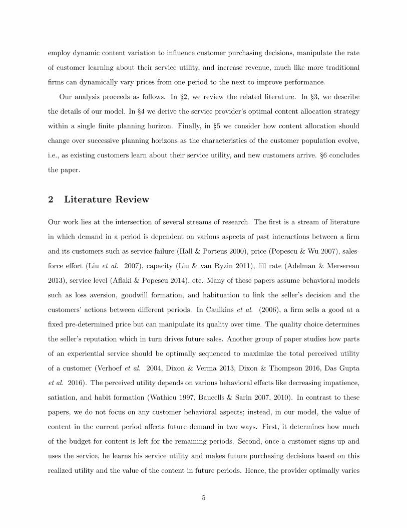
if not always, robust to the number of periods in the planning horizon (see Figure 1).

18

0 1 2 3 4 5 6 7 8Heterogeneity in Utility from Service, σθ

4.2

4.3

4.4

4.5

4.6

4.7

4.8

4.9

5.0

Opt

imal

Con

tent

Valu

e

Period 1Period 2

Period 3Period 4

(a) High Budget: V = 18.

0 1 2 3 4 5 6 7 8Heterogeneity in Utility from Service, σθ

1.5

2.0

2.5

3.0

3.5

4.0

4.5

5.0

Opt

imal

Con

tent

Valu

e

Period 1Period 2

Period 3Period 4

(b) Moderate Budget: V = 14.

Figure 1. Optimal Content Values in T = 4 Periods. In this figure, µ = 10, p = 12, σε = 2, α = 0.5.

Corollary 1. When T = 2, V = 2(p − µ). Hence, in a planning horizon consisting of T = 2

periods:

(i) For a high budget, V > 2(p−µ−xcσε), the optimal values v∗1 and v∗2 intersect only at σθ. Along

with Propositions 3 and 4, this means that the service provider should weakly increase content value

over time for any σθ < σθ, offer equal value, V/2, in both periods when σθ = σθ, and weakly decrease

value over time when σθ > σθ.

(ii) For a moderate value budget, 2(p − µ) < V ≤ 2(p − µ − xcσε), the optimal values v∗1 and v∗2

never intersect at any σθ > 0. Along with Propositions 3 and 4, this means that the service provider

should always weakly decrease content value over time for any σθ.

(iii) For σθ > 0, let σε be the unique positive value of σε that satisfies (7). The service provider

should weakly increase content value over time for any σε < σε, offer equal value, V/2, in both

periods when σε = σε, and weakly decrease value over time when σε > σε.

For the special case of a two period planning horizon, part (i) of Corollary 1 shows that with a

high budget, the optimal content allocation policy is increasing over time for low σθ and decreasing

over time for high σθ, unifying the extreme cases of Propositions 3 and 4. As can be seen from

part (i) of Corollary 1, v∗1 and v∗2 intersect only at σθ = σθ. Hence, for a high budget, σθ represents

the critical level of customer heterogeneity in service value, below which the provider prioritizes

inducing purchases from repeat customers in period 2 and above which it prioritizes inducing new

customers to sign up in period 1. The same intuition also generally holds in a planning horizon

19

0 2 4 6 8 10 12 14 16Heterogeneity in Utility from Content, σε

2

3

4

5

6

7

8

Opt

imal

Con

tent

Valu

ePeriod 1 Period 2

Figure 2. Change in Optimal Content Value with σε. In this figure, σθ = 8, while other parameter values aresame as in Figure 1.

consisting of more than two periods, as illustrated in Figure 1a.

Part (ii) similarly unifies the extreme cases of Propositions 3 and 4 for a moderate budget,

showing that in this case, the service provider always prioritizes gaining new customers in period

1 over inducing purchases from repeat customers in period 2. Figure 1b illustrates that the same

policy is generally optimal when there are more than two periods in the planning horizon.

Part (iii) of Corollary 1 describes the impact of a different type of customer heterogeneity on

the provider’s optimal policy: heterogeneity in customer value for content, σε. In Proposition 2, we

saw that when σθ = 0 and the budget is high (V > V ), the provider should allocate value equally

among all periods, and this result holds for any value of σε. When σθ > 0, the corollary shows

how this changes: the service provider should prioritize garnering repeat usages by increasing the

value allocation over time for low heterogeneity of content value (low σε), and should prioritize sign

ups from new customers early on in the planning horizon by decreasing the value allocation over

time for high heterogeneity of content value (high σε). The behavior described as a function of σε

is qualitatively similar to that described in part (i) of the corollary as a function of σθ. Figure 2

shows the optimal content allocation policy as a function of σε for T = 2. Observe that the point

σε for a fixed σθ is analogous to the point σθ for a fixed σε with one key difference: σθ only exists

for small σε (specifically, σε < (p−µ−V/2)/xc; see part (i) of Corollary 1), while a unique σε exists

for every σθ.

To summarize, the analysis so far illustrates precisely how a service provider can use dynamic

content variation to increase demand, and, moreover, the significant impact that new customers

20

and their ability to learn about service utility have on the provider’s optimal value allocation policy:

any deviation from a constant value allocation is driven by the presence of these new (as opposed

to repeat) customers, and the provider changes its content value over time to balance the rate at

which new customers first try the service in period 1 and the rate at which they continue their

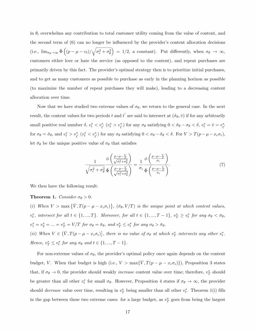
service in period 2. The insights from these results are summarized in Figure 3. Observe that

whenever customers are very heterogeneous in either content utility or service utility, the provider

should use a decreasing content allocation policy, i.e., by beginning with high content value in

period 1 and decreasing it thereafter. Put differently, the provider should focus on acquiring new

customers early in the planning horizon with high value content, but should decrease the value of

that content afterwards, relying instead on customers with particularly high realizations of service

or content value to continue using the service.

On the other hand, when overall heterogeneity is low (i.e., if both σθ and σε are small), the

provider should follow an increasing content allocation policy, i.e., beginning with a relatively

low content value in period 1 and increasing it thereafter. In other words, it should focus on

retaining current customers by offering progressively better content over time. In this case, customer

heterogeneity (in either service or content utility) is too small to drive significant repeat purchases,

so the provider must induce repeat purchases by offering more valuable content in each period.

The critical threshold that governs the transition between these two strategies (represented by

the curve in Figure 3), characterized by σε and σθ—the solutions to (7)—represents the levels of

heterogeneity at which the provider offers equal value in both periods. Accordingly, while intuition

might suggest that service providers should offer constant value content through a planning horizon,

these results show that constant value is only optimal under very specific conditions; in most cases,

the optimal dynamic content allocation is monotonically increasing (if customer heterogeneity is

low) or decreasing (if heterogeneity is high) over time.

5 Optimal Content Allocation Across Planning Horizons

In the preceding section, we derived the service provider’s optimal content allocation policy within a

planning horizon consisting of T ≥ 2 periods. In this section, we consider how the optimal allocation

policy changes over time when there are multiple sequential planning horizons. To streamline our

21

0 5 10 15 20 25 30 35 40Heterogeneity in Service Utility, σθ

0.0

0.5

1.0

1.5

2.0

2.5

3.0

3.5

4.0

Het

erog

enei

tyin

Con

tent

Uti

lity,σε

Content ValueIncreases Over Time

Content ValueDecreases Over Time

Figure 3. Service Provider’s Optimal Value Allocation Policy. All parameter values are same as in Figure 1.

analysis, in this section we restrict attention to planning horizons that consist of two periods (i.e.,

T = 2), but we allow there to be an arbitrary number of successive two-period horizons.

At the beginning of planning horizon k (for k ∈ {1, 2, 3, ...}), the provider receives a budget

V > 2(p − µ) which it then divides between the two periods to maximize expected demand over

horizon k. In other words, we assume that the provider’s budget renews in every planning horizon,

and the provider determines a content allocation policy at the beginning of each planning horizon

to maximize demand (equivalently, revenue) purely within that horizon. Unused budget is lost,

i.e., the horizon k budget can only be used in horizon k. A practical example of this would be

a streaming video service like Netflix employing a fixed budget for each fiscal year, and making

content allocation decisions to maximize revenue for one fiscal year at a time. If the provider is more

forward looking and takes into account the impact of decisions in planning horizon k on demand

in planning horizons k+ 1, k+ 2, etc., its problem would be similar to the general T -period model,

with the difference that it receives a new budget in each horizon (instead of a single budget that

can be arbitrarily allocated in the T period, single-horizon model).

Over successive planning horizons, it is possible that several parameters of the service provider’s

problem, namely, the price, the mean service utility, and the total budget, which we have assumed

to remain constant within a planning horizon, might change. However, these parameters will

generally depend on several external factors including the provider’s market valuation, popularity

of the particular service category, competition within the industry, and the state of the economy,

all of which are outside of our model. Theorem 1 specifies how the provider’s optimal budget

allocation strategy should change with these parameters; for our analysis in this section, and for

ease of exposition, we assume that p, µ, and V are constant across every successive planning horizon.

22

By assuming the service provider “myopically” optimizes demand one planning horizon at a

time, we may directly apply the results from the preceding section to study successive planning

horizons. Despite the fact that the provider’s optimal decisions within horizon k are myopically

determined by their impact on that planning horizon, those decisions do have an important role in

determining the fraction of repeat customers (α) that are present in planning horizon k+ 1. To see

this, note that any new customer who purchases at least once in a planning horizon begins the next

planning horizon as a repeat customer. Hence, decisions in horizon k determine how the customer

population evolves for horizon k + 1.

Because of this, the impact of α on the optimal dynamic content allocation policy is critical in

analyzing successive planning horizons. The following result describes how the provider’s optimal

allocation policy—for a single, two-period planning horizon—and total expected demand change

with α.

Proposition 5. As α increases, the difference between the optimal values in the two periods,

|v∗1(α)− v∗2(α)|, as well as the total expected demand in the planning horizon weakly decrease.

A new customer i initially does not know his service utility θi and purchases in period t ∈ {1, 2}

if the expected service utility satisfies E[uit] = µ + vt − p ≥ 0. Therefore, it is possible that he

signs up, only to experience a negative net utility, i.e., θi + vt− p < 0. On the other hand, a repeat

customer knows his service utility before making a purchasing decision, and will never purchase if

net utility is negative. As α increases, the fraction of new customers decreases, and for the service

provider, the likelihood of “erroneous” purchases from new customers—customers paying the price

p only to realize a negative net utility in a period—declines. Consequently, the provider’s expected

demand decreases with α.

At the same time, as α increases, the provider divides its budget more evenly over time, for two

reasons. First, as we discussed in §4, the principal trade-off that the provider faces while choosing

its optimal content allocation policy in a two-period horizon is whether to induce new customers

to sign up in period 1 by setting a high v1 or to persuade those new customers who signed up in

period 1 to continue their service in period 2 by setting a high v2. As α increases, the importance of

this trade-off decreases since there are fewer new customers in the market. Second, the provider’s

optimal allocation policy when catering to repeat customers is to divide the budget equally in the

23

two periods because of the “S” shape of the demand function (as discussed in Proposition 2). Hence,

when there are fewer new (and more repeat) customers at the beginning of a planning horizon, the

provider employs a more stable content allocation policy; in the extreme case when α = 1, content

value is constant over time.

Having shown how α influences the optimal allocation policy of the provider, we now consider

how the provider’s content decisions in planning horizon k influence α for planning horizon k + 1.

Before doing so, however, it’s important to discuss an issue that may arise with multiple successive

planning horizons. In §4 we assumed that the market size does not change within a planning

horizon; however, the change in market size is likely to be more significant over the course of

multiple planning horizons. Thus, we consider this possibility by allowing additional new customers

to enter the market at the beginning of each planning horizon. These newly arriving customers

have never considered accessing the service in the past (which could be because they became aware

of the service only recently after being exposed to an advertisement, or because the provider has

recently expanded the service to their geographical area), but starting from the planning horizon

in which they arrive, they make the same purchasing decisions as the other new customers who

had entered the market in previous horizons. Consequently, α in horizon k + 1 is determined by

two factors: the mass of new arrivals that enter the market in horizon k + 1, as well the evolution

of the customer population that takes place during horizon k (i.e., the fraction of customers who

learn θi by the end of horizon k).

In what follows, we define the market size in planning horizon k to be Mk, and we suppose

mk+1 new customers enter the market at the beginning of planning horizon k + 1. Then the total

market size in planning horizon k + 1 is Mk+1 = Mk + mk+1. Let αk be the fraction of repeat

customers at the beginning of planning horizon k. We denote the rate of growth in the market size

in planning horizon k + 1 by rk+1, i.e., rk+1 = mk+1/Mk. To consider the different ways in which

αk can evolve, we study the following two special cases: (a) the growth rate, rk, remains constant

over the planning horizons, i.e., the market size grows exponentially; (b) the mass of new arrivals,

mk, remains constant over the planning horizons, i.e., the market size grows linearly.

This leads us to the following result, which details how α evolves over successive planning

horizons.

24

Proposition 6. Suppose the service provider’s optimal value allocation in periods 1 and 2 of plan-

ning horizon k are v∗(αk) and V − v∗(αk), respectively. Then, the fraction of repeat customers at

the beginning of planning horizon k + 1 is

αk+1 =1

1 + rk+1

[1− (1− αk)Φ

(p− µ− v∗(αk)

σε

)Φ

(p− µ− V + v∗(αk)

σε

)]. (8)

(i) If the market size grows at a constant exponential rate, i.e., rk+1 = r > 0 ∀ k, then there exists

a unique α∗ < 1, implicitly defined by

α∗ =1− Φ

(p−µ−v∗(α∗)

σε

)Φ(p−µ−V+v∗(α∗)

σε

)1− Φ

(p−µ−v∗(α∗)

σε

)Φ(p−µ−V+v∗(α∗)

σε

)+ r

(9)

such that αk ≤ α∗ if and only if αk+1 ≥ αk, and if αk = α∗, then αk+1 = α∗.

(ii) If the market size grows at a constant linear rate, i.e., mk+1 = m ≥ 0 ∀ k, then lim k→∞αk = 1.

The first part of the proposition specifies how α changes from one planning horizon to the next

based on the market growth rate and the content values set by the provider. Observe that at the

beginning of planning horizon k, the market consists of αkMk repeat customers and (1 − αk)Mk

new customers. From Proposition 1, Φ(p−µ−v∗(αk)

σε

)Φ(p−µ−V+v∗(αk)

σε

)represents the probability

that a new customer did not sign up in either of the two periods in a planning horizon. Hence,

in planning horizon k, a Φ(p−µ−v∗(αk)

σε

)Φ(p−µ−V+v∗(αk)

σε

)fraction of new customers will still not

sign up for the service, while the complementary fraction use the service and learn θi. Therefore

(ignoring new arrivals in horizon k+1), the fraction of repeat customers increases, while the fraction

of new customers decreases. At the beginning of planning horizon k + 1, a mass mk+1(= rk+1Mk)

of new customers enters the market. These two effects lead to (8).

Part (i) of the proposition shows that with constant exponential growth in market size, it is

possible that the rate at which existing new customers sign up and learn θi is matched by the

rate at which new arrivals enter the market, resulting in a constant α over planning horizons. This

equilibrium α∗, characterized in (9), is such that the market will move towards the equilibrium, and

once at equilibrium, will remain there. From Proposition 5, it follows that in this equilibrium state,

the service provider will always set the same content values in every planning horizon: v∗(α∗) in

period 1 of the planning horizon and V − v∗(α∗) in period 2; hence, content will alternate between

25

0 10 20 30 40 50 60

Period

4.7

4.8

4.9

5.0

5.1

5.2

5.3

Opt

imal

Con

tent

Valu

e

Exponential Growth Constant Growth No Growth

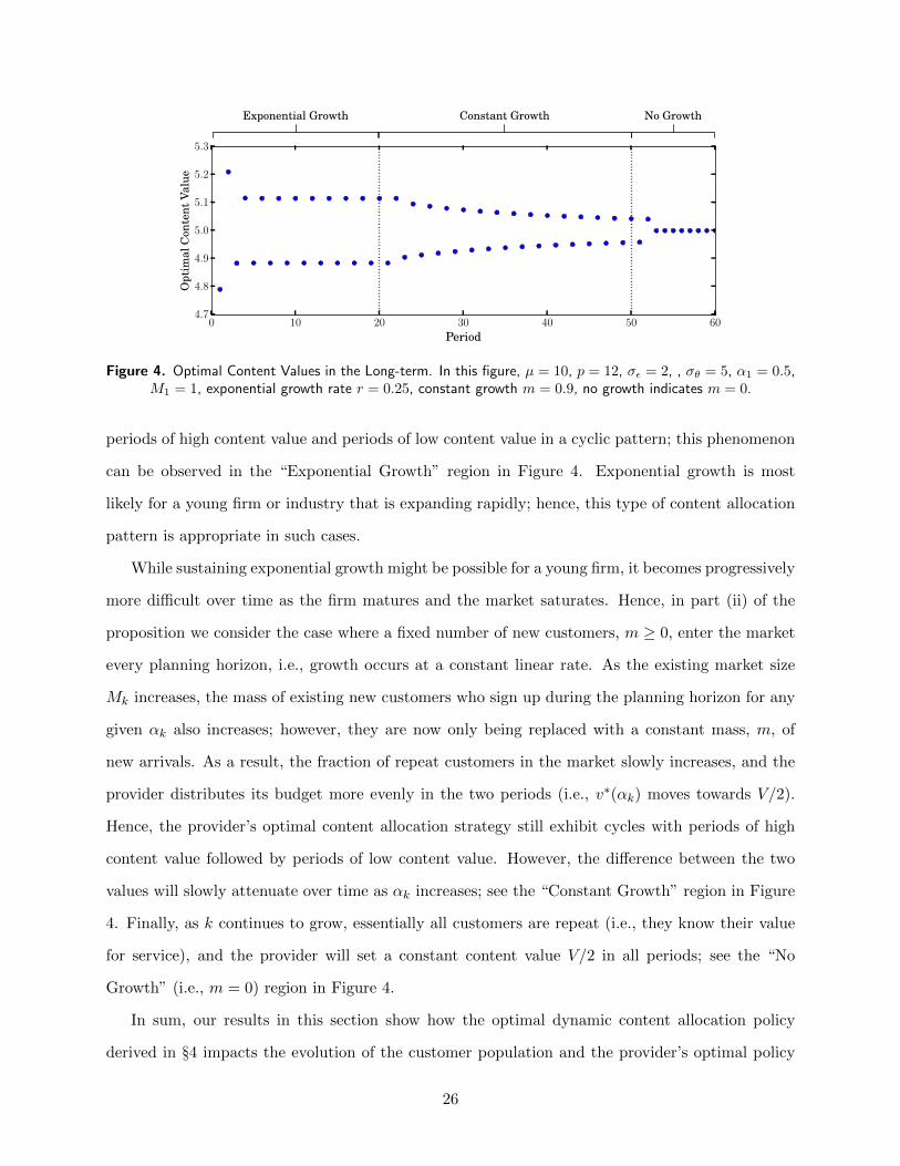
Figure 4. Optimal Content Values in the Long-term. In this figure, µ = 10, p = 12, σε = 2, , σθ = 5, α1 = 0.5,M1 = 1, exponential growth rate r = 0.25, constant growth m = 0.9, no growth indicates m = 0.

periods of high content value and periods of low content value in a cyclic pattern; this phenomenon

can be observed in the “Exponential Growth” region in Figure 4. Exponential growth is most

likely for a young firm or industry that is expanding rapidly; hence, this type of content allocation

pattern is appropriate in such cases.

While sustaining exponential growth might be possible for a young firm, it becomes progressively

more difficult over time as the firm matures and the market saturates. Hence, in part (ii) of the

proposition we consider the case where a fixed number of new customers, m ≥ 0, enter the market

every planning horizon, i.e., growth occurs at a constant linear rate. As the existing market size

Mk increases, the mass of existing new customers who sign up during the planning horizon for any

given αk also increases; however, they are now only being replaced with a constant mass, m, of

new arrivals. As a result, the fraction of repeat customers in the market slowly increases, and the

provider distributes its budget more evenly in the two periods (i.e., v∗(αk) moves towards V/2).

Hence, the provider’s optimal content allocation strategy still exhibit cycles with periods of high

content value followed by periods of low content value. However, the difference between the two

values will slowly attenuate over time as αk increases; see the “Constant Growth” region in Figure

4. Finally, as k continues to grow, essentially all customers are repeat (i.e., they know their value

for service), and the provider will set a constant content value V/2 in all periods; see the “No

Growth” (i.e., m = 0) region in Figure 4.

In sum, our results in this section show how the optimal dynamic content allocation policy

derived in §4 impacts the evolution of the customer population and the provider’s optimal policy

26

over successive planning horizons. Depending on the rate of market growth, the provider could

find itself reaching an equilibrium α < 1 or a boundary α = 1. In either case, as α increases, the

optimal content allocation policy becomes more “even” over time, resulting in patterns like those

in Figure 4.

6 Conclusion

Services where providers have the ability to vary the content over time are becoming more preva-

lent. While many traditional business models involve varying price over time to influence customer

purchasing decisions and maximize revenue, these new services typically operate with a constant

price. This raises the question of how a service provider can use dynamic content variation—as

opposed to dynamic pricing—to maximize demand and revenue. What makes this problem chal-

lenging is that providers typically have limited resources and hence face a constraint on the total

budget for content that they may employ within a planning horizon. Hence, the provider is forced

to trade off the benefit of offering highly valued content in one period (raising demand in that

period) with the cost of offering less valuable content in another period (lowering demand in that

period).

We find that the optimal dynamic content allocation policy is not, in general, to offer content of

equal value over time. Instead, it depends critically on the level of heterogeneity in both components

of utility in the customer population. The optimal policy consists of a monotonically increasing

level of content value over time when heterogeneity is low; in this case, the provider cannot rely on

customer heterogeneity to encourage repeat purchases (i.e., because many customers have especially

high content or service value), and so the provider itself must encourage such purchases by offering

increasingly better content over time. By contrast, when heterogeneity is high, the provider should

monotonically decrease the level of content value over time. In this case, customer heterogeneity

will spur most repeat purchases, so the provider’s goal should be to get as many customers as

possible to experience service for the first time early in a planning horizon, maximizing the number

of opportunities for repeat purchases based on heterogeneous realizations of content or service

utility.

We also analyzed how the service provider’s content allocation policy changes across multiple

27

successive planning horizons. We found that a service that is able to sustain a constant exponential

growth in market size might reach a steady state wherein the rate of new arrivals balances the

rate at which existing new customers use the service and learn their utility. In this steady state,

the market composition and the provider’s optimal value allocation within a planning horizon will

remain constant over each successive planning horizon, leading to cyclic content patterns over time,

i.e., alternating between periods of high content value and periods of low content value. Conversely,

if the service enjoys slower (i.e., constant linear) growth in market size, the provider will not be

able to maintain a constant market composition. Instead, over time the repeat customers will

constitute a progressively larger fraction of the market, and the provider will distribute its content

budget more evenly throughout the planning horizon. Therefore, while content value may start by

alternating between periods of high and low content value, the difference between these two values

will diminish over time.

Taken in sum, our results show how new business models—such as video streaming services

and curated subscription boxes—can lead to new ways for firms to influence customer purchasing

decisions, in our case maximizing revenue by dynamically varying the content of the service over

time, rather than the price of that content. As such business models continue to grow in popularity,

understanding how to use all the levers available to firms to maximize demand will be of increasing

importance. Our model thus provides a first step in this direction by studying optimal dynamic

content variation under customer learning.

References

Adelman, Daniel, & Mersereau, Adam J. 2013. Dynamic Capacity Allocation to Customers Who Remember

Past Service. Management Science, 59(3), 592–612.

Aflaki, Sam, & Popescu, Ioana. 2014. Managing Retention in Service Relationships. Management Science,

60(2), 415–433.

Baucells, Manel, & Sarin, Rakesh K. 2007. Satiation in Discounted Utility. Operations Research, 55(1),

170–181.

Baucells, Manel, & Sarin, Rakesh K. 2010. Predicting Utility Under Satiation and Habit Formation. Man-

agement Science, 56(2), 286–301.

28

Bernstein, Fernando, & Martınez-de Albeniz, Victor. 2017. Dynamic Product Rotation in the Presence of

Strategic Customers. Management Science, 63(7), 2092–2107.

Caro, Felipe, & Martınez-de Albeniz, Victor. 2020. Managing Online Content to Build a Follower Base:

Model and Applications. INFORMS Journal on Optimization, 2(1), 57–77.

Caro, Felipe, Martınez-de Albeniz, Victor, & Rusmevichientong, Paat. 2014. The Assortment Packing

Problem: Multiperiod Assortment Planning for Short-Lived Products. Management Science, 60(11),

2701–2721.

Caulkins, Jonathan P., Feichtinger, Gustav, Haunschmied, Josef, & Tragler, Gernot. 2006. Quality Cycles

and the Strategic Manipulation of Value. Operations Research, 54(4), 666–677.

Das Gupta, Aparupa, Karmarkar, Uday S., & Roels, Guillaume. 2016. The Design of Experiential Services

with Acclimation and Memory Decay: Optimal Sequence and Duration. Management Science, 62(5),

1278–1296.

Desai, Preyas S. 2001. Quality segmentation in spatial markets: When does cannibalization affect product

line design? Marketing Science, 20(3), 265–283.

Digital Trends. 2020. What’s new on Netflix, and what’s leaving in June 2020.

Dixon, Michael, & Verma, Rohit. 2013. Sequence effects in service bundles: Implications for service design

and scheduling. Journal of Operations Management, 31(3), 138–152.

Dixon, Michael J., & Thompson, Gary M. 2016. Bundling and Scheduling Service Packages with Customer

Behavior: Model and Heuristic. Production and Operations Management, 25(1), 36–55.

Engadget. 2018. Apple Music makes it easier to see new albums that are on the way.

Feldman, Pnina, Papanastasiou, Yiangos, & Segev, Ella. 2019. Social Learning and the Design of New

Experience Goods. Management Science, 65(4), 1502–1519.

Ferreira, Kris, & Goh, Joel. 2018. Assortment Rotation and the Value of Concealment. Working Paper.

Forbes. 2018. Exclusive: 60% Of U.S. Amazon Customers Will Not Renew Their Prime Membership, Poll

Reveals.

Forbes. 2019. Analysis: Here’s why Netflix won’t raise prices again in 2020.

Hall, Joseph, & Porteus, Evan. 2000. Customer Service Competition in Capacitated Systems. Manufacturing

& Service Operations Management, 2(2), 144–165.

Jerath, Kinshuk, Kim, Sang-Hyun, & Swinney, Robert. 2017. Product quality in a distribution channel with

inventory risk. Marketing Science, 36(5), 747–761.

Liu, Ben Shaw-Ching, Petruzzi, Nicholas C., & Sudharshan, D. 2007. A service effort allocation model for

assessing customer lifetime value in service marketing. Journal of Services Marketing, 21(1), 24–35.

29

Liu, Qian, & van Ryzin, Garrett. 2011. Strategic Capacity Rationing when Customers Learn. Manufacturing

& Service Operations Management, 13(1), 89–107.

Mussa, Michael, & Rosen, Sherwin. 1978. Monopoly and product quality. Journal of Economic theory,

18(2), 301–317.

Popescu, Ioana, & Wu, Yaozhong. 2007. Dynamic Pricing Strategies with Reference Effects. Operations

Research, 55(3), 413–429.

Sundaram, Rangarajan K. 1996. A First Course in Optimization Theory. Cambridge University Press.

Talluri, Kalyan T, & Van Ryzin, Garrett J. 2006. The theory and practice of revenue management. Vol. 68.

Springer Science & Business Media.

USA Today. 2019. Netflix price increases could cause some subscribers to downgrade, cancel streaming

service.

Verhoef, Peter C., Antonides, Gerrit, & de Hoog, Arnoud N. 2004. Service Encounters as a Sequence of

Events: The Importance of Peak Experiences. Journal of Service Research, 7(1), 53–64.

Wathieu, Luc. 1997. Habits and the Anomalies in Intertemporal Choice. Management Science, 43(11),

1552–1563.

30

Online Supplement to “Dynamic Content Variation with Customer

Learning”

A Appendix: Proof of Results

Proof of Proposition 1: We prove (4) by induction. Observe that a repeat customer i who hasused the service in a previous planning horizon and already knows θi before period 1 will use theservice in period t ∈ {1, 2, ..., T} only if uit = θi + vt + εit − p ≥ 0. Since θi + εit ∼ N(µ, σ2

ε + σ2θ),

from the provider’s perspective before period 1, customer i will use the service in period t with

probability Φ

(p−µ−vt√σ2ε+σ2

θ

). On the other hand, an initially (i.e., before period 1) new customer j

will sign up for the service in period t if E[ujt] = µ + vt + εjt − p ≥ 0, i.e., if εjt ≥ p − µ − vt.Since εjt ∼ N(0, σ2

ε ) from the provider’s perspective before period 1, customer j will sign up

in period t with probability Φ(p−µ−vtσε

). Since the market consists of an α fraction of repeat

customers and a 1−α fraction of new customers, total expected demand when T = 1 is E[D]|T=1 =

αΦ

(p−µ−v1√σ2ε+σ2

θ

)+ (1− α)Φ

(p−µ−v1

σε

). Thus, (4) holds when T = 1.

Suppose that (4) also holds for T − 1 for any T > 2. Hence, total expected demand in periods1 to T − 1 is E[D]|T−1 =

= α

T−1∑t=1

Φ

(p− µ− vt√σ2ε + σ2

θ

)+ (1− α)

[1−

T−1∏t=1

Φ

(p− µ− vt

σε

)+

T−1∑t=2

Φ

(p− µ− vt√σ2ε + σ2

θ

){1−

t−1∏i=1

Φ

(p− µ− vi

σε

)}].

Expected demand in period T from customers who are new at the beginning of the horizon is givenby

E[DNT ] = Φ

p− µ− vT√σ2ε + σ2

θ

[1−T−1∏i=1

Φ

(p− µ− vi

σε

)]+ Φ

(p− µ− vT

σε

) T−1∏i=1

Φ

(p− µ− vi

σε

).

(A.1)The first term is the probability that a new customer used the service at least once in the firstT − 1 periods and is using it again in period T , while the second term is the probability that a newcustomer who has never used the service before is using it for the first time in period T . Hence,

the total expected demand in period T is E[DT ] = αΦ

(p−µ−vT√σ2ε+σ2

θ

)+ (1 − α)E[DN

T ]. Observe that

E[D]|T = E[D]|T−1 + E[DT ]. Hence, by induction, (4) holds for any T .

Proof of Proposition 2: When σθ = 0, the total expected demand in (4) reduces to

E[D] = ΣTt=1Φ

(p− µ− vt

σε

).

We divide the proof into the following lemmas.

1

Lemma A.1. Assume σθ = 0. If µ + VT > p, then v∗t = V

T ∀ t ∈ {1, 2, ..., T} is a strict localmaximum to the provider’s problem.

Proof. The provider solves the constrained optimization problem: Maximize E[D] subject to ΣTt=1vt =

V . Define the Lagrangian, L = E[D] + λ(V − ΣTt=1vt), where the Lagrangian multiplier, λ ≥ 0.

∂L∂vt

= 0 implies φ(p−µ−vtσε

)= σελ for all t ∈ {1, ..., T}. Let x∗ ≥ 0 be such that φ(x∗) = σελ. Note

that there could be three possible cases.Case 1:

p−µ−v∗tσε

= −x∗ ≤ 0 for all t ∈ {1, ..., T}. This implies that the provider sets value

v∗t = p− µ+ x∗σε in all periods. From∑T

t=1 v∗t = V , x∗ =

µ+VT−p

σε. Hence, x∗ ≥ 0 is possible only

if µ + VT ≥ p. Therefore, v∗t = V

T and λ∗ = 1σεφ

(µ+V

T−p

σε

). To study the second order condition,

we follow Theorem 5.4 of Sundaram (1996), and define a set of vectors

Z =

{z ∈ RT

∣∣∣∣∣[∂

∂v1

(V −

T∑t=1

vt

), ...,

∂

∂vT

(V −

T∑t=1

vt

)]z = 0

}=

{z ∈ RT

∣∣∣∣∣T∑t=1

zt = 0

}.

Further observe that the second derivative, D2L(v∗, λ∗), is a diagonal matrix with elementsp−µ−v∗tσ3ε

φ(p−µ−v∗t

σε

)≤ 0 (since, v∗t = V

T ≥ p− µ). This is a local maximum because

z′D2L(v∗, λ∗)z =

T∑t=1

z2t

p− µ− v∗tσ3ε

φ

(p− µ− v∗t

σε

)≤ 0.

Case 2:p−µ−v∗t

σε= x∗ ≥ 0 for all t ∈ {1, ..., T}. Therefore, v∗t = p − µ − x∗σε in all periods.

From∑T

t=1 v∗t = V , x∗ = −µ+V

T−p

σε. Hence, x∗ ≥ 0 is possible only if µ + V

T ≤ p. Therefore,

v∗t = VT and λ∗ = 1

σεφ

(−µ+V

T−p

σε

). The second derivative test now results in z

′D2L(v∗, λ∗)z =∑T

t=1 z2tp−µ−v∗tσ3ε

φ(p−µ−v∗t

σε

)≥ 0. Hence, this is a local minimum.

Case 3: Now suppose, without loss of generality,p−µ−v∗t

σε= x∗ for k ∈ {1, ..., T − 1} periods

andp−µ−v∗t

σε= −x∗ for the remaining T − k periods. In this case, x∗ =

µ+VT−p

(1−2 kT

)σεand λ∗ =

1σεφ

(µ+V

T−p

(1−2 kT

)σε

), which is neither a minimum nor a maximum. Indeed, consider zt = γ(> 0) for

one of the k periods withp−µ−v∗t

σε= x∗, zt = 0 for the other k − 1 periods with

p−µ−v∗tσε

= x∗

and zt = − γT−k for each of the T − k periods with

p−µ−v∗tσε

= −x∗. We have z′D2L(v∗, λ∗)z =

x∗φ(x∗)σ2ε

[γ2 − (T − k) γ2

(T−k)2

]≥ 0. Now consider z such that zt = γ(> 0) for one of the T−k periods

withp−µ−v∗t

σε= −x∗, zt = 0 for the remaining T − k − 1 periods with

p−µ−v∗tσε

= −x∗ and zt = −γk

for each of the k periods withp−µ−v∗t

σε= x∗. Then, z

′D2L(v∗, λ∗)z = x∗φ(x∗)

σ2ε

[−γ2 + k γ

2

k2

]≤ 0.

Lemma A.2. There exists a threshold, V , such that v∗t = VT ∀ t ∈ {1, 2, ..., T} is the unique global

maximum for any V > V .

Proof. Observe that we have ignored the constraints vt ≥ 0 ∀ t ∈ {1, ...T} in our analysis above.

2

Now suppose we impose this constraint by making some of the vt to be zero. From Lemma A.1, itfollows that an allocation with v∗t = V

k for any k periods, where k ∈ {1, 2, ..., T − 1} and v∗t = 0 inthe remaining T −k periods is also a strict local maximum when µ+ V

T > p (since µ+ Vk > p). The

allocation, v∗t = VT ∀ t ∈ {1, 2, ..., T} is the unique global maximum if, for any k ∈ {1, 2, ..., T − 1}

kΦ

(p− µ− V

k

σε

)+ (T − k)Φ

(p− µσε

)< T Φ

(p− µ− V

T

σε

). (A.2)

Observe that as V increases, the right-hand side of (A.2) increases faster than the left-hand side forany k < T . Moreover, as V →∞, the inequality in (A.2) holds. Therefore, there exists a unique V

′

such that (A.2) holds for any V > V′

and v∗t = VT ∀ t ∈ {1, 2, ..., T} is the unique global maximum

for any V > max{V ′ , T (p− µ)} ≡ V .

Proof of Proposition 3 : We provide a proof by contradiction. Suppose the optimal solutionallocates vH in period k and vL(< vH) in period k+1 for any k ∈ {1, 2, ..., T −1} and achieves totalexpected demand E[D]HL. Consider an allocation where we switch the content values in periods kand k + 1 (i.e., vk = vL and vk+1 = vH) while keeping all other periods unchanged. Let the newtotal expected demand be E[D]LH . From (4), note that E[D]LH − E[D]HL =

= (1− α)

k−1∏i=1

Φ

(p− µ− vi

σε

)Φ

p− µ− vH√σ2ε + σ2

θ

Φ

(p− µ− vL

σε

)− Φ

p− µ− vL√σ2ε + σ2

θ

Φ

(p− µ− vH

σε

) . (A.3)

Observe that if ∂∂σ

Φ(p−µ−vH

σ

)Φ(p−µ−vL

σ

)∣∣∣∣∣σ=σε

> 0, then E[D]LH−E[D]HL > 0 when σθ is infinitesimally small.

Now,

∂

∂σ

Φ(p−µ−vH

σ

)Φ(p−µ−vL

σ

) ∣∣∣∣∣σ=σε

=1

σε

Φ(p−µ−vH

σ

)Φ(p−µ−vL

σ

)p− µ− vH

σε

φ(p−µ−vH

σε

)Φ(p−µ−vH

σε

) − p− µ− vLσε

φ(p−µ−vL

σε

)Φ(p−µ−vL

σε

) .

For standard normal, the generalized failure rate x φ(x)Φ(x)

decreases in (−∞, xc] and increases in

[xc,+∞), where xc ≈ −0.84 is the unique solution to Φ(x) − x2Φ(x) + xφ(x) = 0. Therefore,

a sufficient condition for ∂∂σ

Φ(p−µ−vH

σ

)Φ(p−µ−vL

σ

)∣∣∣∣∣σ=σε

> 0 is p−µ−vLσε

< xc, i.e., vL > p − µ − xcσε. From

Proposition 2, note that when σθ = 0, v∗t = VT as long as V > V ≥ T (p − µ). Since (4) is

right continuous at σθ = 0, there exist small positive γ, δ such that when σθ < γ, both∣∣∣VT −

vL

∣∣∣ < δ and∣∣∣VT − vH

∣∣∣ < δ hold. Hence, when σθ → 0 and V > max{V , T (p− µ− xcσε)

},

p−µ−VT

σε< xc; consequently, p−µ−vL

σε< xc holds and E[D]LH > E[D]HL. Therefore, the provider

is better off with the new allocation. Using the same logic for any k, vL, and vH , we concludethat only weakly increasing value paths can be optimal. The opposite argument holds when V ∈(V , T (p− µ− xcσε)

). In this case, a sufficient condition for ∂

∂σ

Φ(p−µ−vH

σ

)Φ(p−µ−vL

σ

)∣∣∣∣∣σ=σε

< 0 is p−µ−vHσε

> xc,

3

i.e., vH < p−µ−xcσε. Note that V < T (p−µ−xcσε) implies p−µ−vHσε

> xc; so E[D]LH < E[D]HL,and only weakly decreasing value paths can be optimal.

Proof of Proposition 4: We again provide a proof through contradiction. Suppose the optimalsolution to the provider’s problem allocates vL in period k and vH(> vL) in period k + 1 for anyk ∈ {1, 2, ..., T − 1} and achieves total expected demand E[D]LH . Now consider another allocationwhere we switch the content values in periods k and k + 1 (i.e., vk = vH and vk+1 = vL) whilekeeping all other periods unchanged. Let the new total expected demand be E[D]HL. The difference

in expected demand, E[D]HL−E[D]LH can be noted from (A.3). When σθ →∞, Φ

(p−µ−v√σ2ε+σ2

θ

)→ 1

2

for any v. Hence,

limσθ→∞

E[D]HL−E[D]LH =1

2(1−α)Πk−1

i=1 Φ

(p− µ− vi

σε

)[Φ

(p− µ− vH

σε

)− Φ

(p− µ− vL

σε

)]> 0.

Therefore, the provider will be better off with the new allocation and the original allocation cannotbe optimal. Moreover, using the same logic for any k, vL, and vH , we conclude that only weaklydecreasing paths can be optimal.

Proof of Theorem 1: We break down the proof into the following lemmas.

Lemma A.3. Suppose the optimal solution to the provider’s problem has vk in period k. Let

R(v, σθ) =Φ

(p−µ−v√σ2ε+σ2

θ

)Φ(p−µ−vσε

) . Then, R(vk, σθ) ≤ R(vk+1, σθ) ∀ k ∈ {1, 2, ..., T − 1}.

Proof. Suppose the optimal solution to the provider’s problem has content values vk and vk+1 inperiods k and k + 1 respectively and results in overall expected demand E[D]. Let E[D]k+1,k bethe demand from an alternate allocation that has vk+1 in period k and vk in period k + 1 whilekeeping all other periods unchanged. Note that E[D]− E[D]k+1,k =

= (1− α)

k−1∏i=1

Φ

(p− µ− vi

σε

)[Φ

(p− µ− vk+1√

σ2ε + σ2

θ

)Φ

(p− µ− vk

σε

)− Φ

(p− µ− vk√σ2ε + σ2

θ

)Φ

(p− µ− vk+1

σε

)].

Since, the allocation with vk in period k and vk+1 in period k+ 1 is optimal, E[D] ≥ E[D]k+1,k

which can be the case only if R(vk, σθ) ≤ R(vk+1, σθ).

Lemma A.4. (i) Let xc ≈ −0.84 be the unique solution to Φ(x)−x2Φ(x) +xφ(x) = 0. For a fixedσθ, R(v, σθ) is quasiconvex in v. When p − µ − xcσε ≥ 0, R(v, σθ) has a unique minimum, v(σθ),that satisfies limσθ→0 v(σθ) = p − µ − xcσε. When p − µ − xcσε < 0, a unique minimum, v(σθ),

only exists when σθ is sufficiently large and satisfies p−µ√σ2ε+σ2

θ

φ

(p−µ√σ2ε+σ2

θ

)

Φ

(p−µ√σ2ε+σ2

θ

) ≥ p−µσε

φ(p−µσε

)Φ(p−µσε

) ; otherwise,

R(v, σθ) is strictly increasing in v. Whenever the minimum, v(σθ), exists, it increases with σθ.(ii) There always exists a unique σθ > 0 satisfying (7) for any V > T (p− µ− xcσε).

4

Proof. (i) Note again that x φ(x)Φ(x)

decreases in (−∞, xc] and increases in [xc,+∞). Now,

∂

∂vR(v, σθ) =

Φ

(p−µ−v√σ2ε+σ2

θ

)Φ(p−µ−vσε

) 1√

σ2ε + σ2

θ

φ

(p−µ−v√σ2ε+σ2

θ

)Φ

(p−µ−v√σ2ε+σ2

θ

) − 1

σε

φ(p−µ−vσε

)Φ(p−µ−vσε

) (A.4)

=1

p− µ− v

Φ

(p−µ−v√σ2ε+σ2

θ

)Φ(p−µ−vσε

) p− µ− v√

σ2ε + σ2

θ

φ

(p−µ−v√σ2ε+σ2

θ

)Φ

(p−µ−v√σ2ε+σ2

θ

) − p− µ− vσε

φ(p−µ−vσε

)Φ(p−µ−vσε

) . (A.5)

First suppose p − µ − xcσε ≥ 0. There can be two cases: 0 < p−µ√σ2ε+σ2

θ

< p−µσε

or xc ≤ p−µσε

<

p−µ√σ2ε+σ2

θ

< 0. From (A.5), note that in both cases, ∂∂vR(v, σθ)

∣∣v=0

< 0. Moreover from (A.5),

∂∂vR(v, σθ)|v=p−µ−xcσε < 0 while ∂

∂vR(v, σθ) > 0 for any v ≥ p − µ − xc√σ2ε + σ2

θ . For standard

normal, the failure rate φ(x)Φ(x)

is increasing in x. As v increases, p−µ−vσεdecreases faster than p−µ−v√

σ2ε+σ2

θ

.

Hence, from (A.4), there exists a unique minimum v(σθ) ∈(p− µ− xcσε, p− µ− xc

√σ2ε + σ2

θ

);

i.e., p−µ−v(σθ)σε

< xc < p−µ−v(σθ)√σ2ε+σ2

θ

< 0. When σθ → 0, ∂∂vR(v, σθ) = 0 is only possible if

limσθ→0 v(σθ) = p − µ − xcσε. For a general σθ,p−µ−v(σθ)√

σ2ε+σ2

θ

φ

(p−µ−v(σθ)√

σ2ε+σ2

θ

)

Φ

(p−µ−v(σθ)√

σ2ε+σ2

θ

) = p−µ−v(σθ)σε

φ(p−µ−v(σθ)

σε

)Φ(p−µ−v(σθ)

σε

) .

If we fix v at v(σθ) and slightly increase σθ,p−µ−v(σθ)√

σ2ε+σ2

θ

increases. Since p−µ−v(σθ)√σ2ε+σ2

θ

∈ (xc, 0), the left

hand side of the above equality increases. Now, p−µ−v(σθ)σε

< xc, implies that v(σθ) must increaseto preserve equality. Hence, v(σθ) increases with σθ.

Next suppose p − µ − xcσε < 0. In this case, for small σθ,p−µσε

< p−µ√σ2ε+σ2

θ

≤ xc; hence,

∂∂vR(v, σθ)

∣∣v=0

> 0. Similarly, for any v > 0, p−µ−vσε

< p−µ−v√σ2ε+σ2

θ

< xc; hence, ∂∂vR(v, σθ) > 0 for any

v > 0 and R(v, σθ) is strictly increasing in v. On the other hand, if σθ is large enough such that

p−µσε

< xc <p−µ√σ2ε+σ2

θ

< 0 and p−µ√σ2ε+σ2

θ

φ

(p−µ√σ2ε+σ2

θ

)

Φ

(p−µ√σ2ε+σ2

θ

) ≥ p−µσε

φ(p−µσε

)Φ(p−µσε

) , we have that ∂∂vR(v, σθ)

∣∣v=0≤ 0.

As v increases, p−µ−v√σ2ε+σ2

θ

φ

(p−µ−v√σ2ε+σ2

θ

)

Φ

(p−µ−v√σ2ε+σ2

θ

) decreases, while p−µ−vσε

φ(p−µ−vσε

)Φ(p−µ−vσε

) increases. Therefore, once σθ

is above a threshold, we have a unique minimum v(σθ) that starts at 0 and increases with σθ.(ii) From (A.4), observe that (7) implies v(σθ) = V/T . We showed in part (i) that when

p− µ− xcσε ≥ 0, limσθ→0 v(σθ) = p− µ− xcσε and v(σθ) increases with σθ; otherwise, there existsa threshold σθ, such that v(σθ) = 0 at the threshold and increases with σθ beyond the threshold.Moreover, from (A.5), note that limσθ→∞

∂∂vR(V/T, σθ) < 0. Hence, following the proof of part (i),

v(σθ) > V/T for very large σθ. Therefore, whenever V > T (p− µ− xcσε), a unique positive σθsatisfying v(σθ) = V/T always exists.

5

Lemma A.5. Suppose there exists a σθ and periods k and k′(< k), such that the optimal allocation

for these two periods intersect at σθ. Then, at σθ, vi = v(σθ) ∀ i ∈ {1, 2, ..., k}.

Proof. We define “intersection” before Theorem 1. First consider the case where for any arbitrarilysmall positive real number δ, vk > vk′ for any σθ satisfying 0 < σθ − σθ < δ and vk < vk′ forany σθ satisfying 0 < σθ − σθ < δ. Lemma A.3 states that for an optimal allocation, R(vk′ , σθ) ≤R(vk, σθ) ∀ k

′< k. From Lemma A.4(i), observe that for a given σθ, R(v, σθ) is either strictly

increasing in v or has a unique minimum, v(σθ). If R(v, σθ) is strictly increasing in v, vk < vk′

would result in R(vk′ , σθ) > R(vk, σθ); hence, an intersection cannot occur. Therefore, we focus onthe case where the unique minimum, v(σθ), exists.

For any σθ satisfying 0 < σθ − σθ < δ, both vk > vk′ and R(vk′ , σθ) ≤ R(vk, σθ) can only betrue if vk > v(σθ). Similarly, for any 0 < σθ − σθ < δ, both vk < vk′ and R(vk′ , σθ) ≤ R(vk, σθ)can only be true if vk < v(σθ). Since the optimal allocation and v(σθ) are continuous in σθ, at σθ,vk = vk′ = v(σθ). Now consider the optimal allocation vk′′ for any period k

′′< k. To preserve,

R(vk′′ , σθ) ≤ R(vk, σθ), vk′′ = v(σθ) must also hold at σθ = σθ. The same argument will be true inthe case where vk < vk′ for any σθ satisfying 0 < σθ − σθ < δ and vk > vk′ for any σθ satisfying0 < σθ − σθ < δ.

First suppose V ∈ (V , T (p− µ− xcσε)]. From Lemma A.5 if follows that if vT intersects vt forany t < T at σθ, v

∗1 = v∗2 = ... = v∗T = v(σθ) = V

T . From Lemma A.4, limσθ→0 v(σθ) = p− µ− xcσεand v(σθ) increases with σθ. Since V

T < p−µ−xcσε ≤ v(σθ) for any σθ > 0, no point of intersectionexists where vT crosses vt for any t < T (see Figure 1b). On the other hand, if V > T (p−µ−xcσε),it follows from (A.4) that the unique σθ, denoted by σθ, at which vT intersects vt for any t < T , isgiven by the solution to (7) (see Figure 1a). Hence, the result follows.

Proof of Corollary 1: When T = 2 and σθ = 0, we can substitute v2 = V − v1 and observe that

v∗1 = V/2 is the unique global maximum to E[D] = Φ(p−µ−v1

σε

)+Φ

(p−µ−v2

σε

)for any V > 2(p−µ).

Hence, when T = 2, the threshold on budget is V = 2(p− µ).Parts (i) and (ii) of the corollary follow from Theorem 1 due to the fact that when T = 2,

v1 = v2 = V2 at any intersection of the content value trajectories.

For part (iii), we fix σθ > 0 and vary σε. When σε = 0, all new customers would sign up in period1 as long as µ+ v1− p ≥ 0; otherwise, they would all sign up in period 2 (since µ+V − v1− p > 0).Hence, the total expected demand (4) becomes

E[D] = α

[Φ

(p− µ− v1

σθ

)+ Φ

(p− µ− v2

σθ

)]+ (1− α)

[1 + Iµ+v1−p≥0Φ

(p− µ− v2

σθ

)](A.6)

where Iµ+v1−p≥0 is 1 if µ+ v1 − p ≥ 0, and 0 otherwise.For σε = 0, we prove v∗1 ≥ v∗2 through contradiction using arguments similar to the proof of

Proposition 3. Suppose the optimal solution to the provider’s problem allocates vL in period 1and vH(> vL) in period 2 and achieves total expected demand E[D]LH . Now consider anotherallocation with v1 = vH and v2 = vL that achieves total expected demand E[D]HL. From (A.6),

E[D]LH − E[D]HL = (1− α)

[Iµ+vL−p≥0Φ

(p− µ− vH

σθ

)− Φ

(p− µ− vL

σθ

)].

6

Observe that for any µ+vL−p ≥ 0, E[D]LH > E[D]HL. But if µ+vL−p < 0, then E[D]LH < E[D]HL

where, E[D]HL = Φ(p−µ−vL

σθ

)+αΦ

(p−µ−vH

σθ

)+1−α. In this case, dE[D]HL

dvL= 1

σθ

[φ(p−µ−vL

σθ

)− αφ

(p−µ−vH

σθ

)].

Now, µ + V/2 − p > 0 implies∣∣∣p−µ−vLσθ

∣∣∣ < ∣∣∣p−µ−vHσθ

∣∣∣; hence, φ(p−µ−vL

σθ

)> φ

(p−µ−vH

σθ

)and

dE[D]HLdvL

> 0. Therefore, when σε = 0, an allocation where vL satisfies µ + vL − p < 0 cannot beoptimal. Consequently, µ + vL − p ≥ 0 and E[D]LH > E[D]HL. Hence when σε = 0, the content

value should weakly increase over time. On the other hand, observe that for any σε ≥ p−µ−V/2xc

,V ≤ 2(p−µ− xcσε); therefore, from Theorem 1 we have, v∗1 ≥ v∗2. Hence, the content value should

weakly decrease over time for any σε ≥ p−µ−V/2xc

.For intermediate σε, we provide a proof similar to that of Theorem 1. For a fixed σθ > 0, let

R(v, σε) =Φ

(p−µ−v√σ2ε+σ2

θ

)Φ(p−µ−vσε

) . We showed in Lemma A.3 that in any optimal allocation, R(v1, σε) ≤

R(v2, σε). From (A.5), note that when p−µσε

> xc,∂∂vR(v, σε)

∣∣v=0

< 0. On the other hand, ifp−µ√σ2ε+σ2

θ

< xc,∂∂vR(v, σε)

∣∣v=0

> 0. Furthermore, for any v > 0, p−µ−vσε

< p−µ−v√σ2ε+σ2

θ

< xc. Hence,

∂∂vR(v, σε) > 0. Now, if we increase σε such that p−µ

σε< xc <

p−µ√σ2ε+σ2

θ

< 0 and p−µ√σ2ε+σ2

θ

φ

(p−µ√σ2ε+σ2

θ

)

Φ

(p−µ√σ2ε+σ2

θ

) >

p−µσε

φ(p−µσε

)Φ(p−µσε

) , then ∂∂vR(v, σε)

∣∣v=0

< 0 holds.

Suppose, ∂∂vR(v, σε)

∣∣v=0

< 0. As v increases, p−µ−vσε

decreases faster than p−µ−v√σ2ε+σ2

θ

. Hence,

from (A.4), there exists a unique minimum v(σε) > 0. At the minimum, p−µ−v(σε)√σ2ε+σ2

θ

φ

(p−µ−v(σε)√

σ2ε+σ2

θ

)

Φ

(p−µ−v(σε)√

σ2ε+σ2

θ

) =

p−µ−v(σε)σε

φ(p−µ−v(σε)

σε

)Φ(p−µ−v(σε)

σε

) . Hence, p−µ−v(σε)σε

< xc <p−µ−v(σε)√

σ2ε+σ2

θ

. Observe that as σε increases, keeping

v fixed at v(σε),p−µ−v(σε)

σεincreases at a faster rate than p−µ−v(σε)√

σ2ε+σ2

θ

. Hence, to preserve the above

inequality, v(σε) must increase with σε. Therefore, whenever σε is sufficiently large, R(v, σε) has aminimum, v(σε), that is unique and increases with σε. From Lemma (A.5), observe that an inter-section can only occur at a minimum, v(σε). Since v(σε) increases with σε, and at any intersectionv1 = v2 = V

2 , an intersection will only occur at the unique value of σε, σε, satisfying (7) for T = 2.Therefore, content values should be weakly increasing for σε < σε, weakly decreasing for σε > σε,and they only intersect at σε = σε.

Proof of Proposition 5: We start with the effect of α on the provider’s optimal allocation. Letthe total expected demand over the planning horizon from new customers be E[DN ]. Hence, thetotal expected demand in the planning horizon is

E[D](α) = α

Φ

p− µ− v1√σ2ε + σ2

θ

+ Φ

p− µ− V + v1√σ2ε + σ2

θ

+ (1− α)E[DN ].

7

For any α, the optimal values, v∗1(α) and V − v∗1(α), must be such that dE[D](α)dv1

∣∣∣∣∣v∗1(α)

=

= (1−α)dE[DN ]

dv1

∣∣∣∣∣v∗1(α)

+α√

σ2ε + σ2

θ

φp− µ− v1√

σ2ε + σ2

θ

− φp− µ− V + v1√

σ2ε + σ2

θ

∣∣∣∣∣v∗1(α)

= 0. (A.7)

Since µ+V/2−p > 0, for any v1 < V/2,∣∣∣ p−µ−v1√

σ2ε+σ2

θ

∣∣∣ < ∣∣∣p−µ−V+v1√σ2ε+σ2

θ

∣∣∣; consequently, φ

(p−µ−v1√σ2ε+σ2

θ

)>

φ

(p−µ−V+v1√

σ2ε+σ2

θ

). Therefore, for any v∗1(α) < V/2, d

dv1

[Φ

(p−µ−v1√σ2ε+σ2

θ

)+ Φ

(p−µ−V+v1√

σ2ε+σ2

θ

)] ∣∣∣∣∣v∗1(α)

> 0,

while dE[DN ]dv1

∣∣∣v∗1(α)

< 0. From (A.7) it also follows thatdv∗1(α)dα = −

∂2E[D](α)∂v1∂α

∣∣∣v∗1(α)

∂2E[D](α)

∂v21

∣∣∣v∗1(α)

. Since v∗1(α) is a

local maximum, ∂2E[D](α)∂v2

1

∣∣∣v∗1(α)

< 0. On the other hand, dE[DN ]dv1

∣∣∣v∗1(α)

< 0 and

ddv1

[Φ

(p−µ−v1√σ2ε+σ2

θ

)+ Φ

(p−µ−V+v1√

σ2ε+σ2

θ

)] ∣∣∣∣∣v∗1(α)

> 0 imply ∂2E[D](α)∂v1∂α

∣∣∣v∗1(α) > 0. Therefore, for any

v∗1(α) < V/2,dv∗1(α)dα > 0. However, if v∗1(α) > V/2, d

dv1

[Φ

(p−µ−v1√σ2ε+σ2

θ

)+ Φ

(p−µ−V+v1√

σ2ε+σ2

θ

)] ∣∣∣v∗1(α)

< 0,

while dE[DN ]dv1

∣∣∣v∗1(α)

> 0. Using similar arguments, we conclude that for any v∗1(α) > V/2,dv∗1(α)dα < 0.

Therefore, as α increases, v∗1(α) moves closer to V/2, and |v∗1(α)− v∗2(α)| weakly decreases.Next focus on the effect of α on the total expected demand. First observe from (4) that new

customer demand when v∗1 = V/2 is

E[DN ]|v∗1=V/2 = 1− Φ2

(p− µ− V

2

σε

)+ Φ

p− µ− V2√

σ2ε + σ2

θ

Φ

(p− µ− V

2

σε

)≥ 2Φ

p− µ− V2√

σ2ε + σ2

θ

.

The last inequality follows from the fact that for any µ+V/2 > p, Φ

(p−µ−V

2√σ2ε+σ2

θ

)+Φ

(p−µ−V

2σε

)≤ 1.

Let us again start with the case where v∗1(α) < V/2. We showed above that for this range

of v∗1(α), v∗1(α) weakly increases with α and the new customer demand dE[DN ]dv1

∣∣∣v∗1(α)

< 0. From

Proposition 2, it follows that v∗1(α = 1) = V/2. Therefore for any α ≤ 1,

E[DN ]|v∗1(α) ≥ E[DN ]|V/2 ≥ 2Φ

p− µ− V2√

σ2ε + σ2

θ

. (A.8)

Additionally, when v∗1(α) < V/2, ddv1

[Φ

(p−µ−v1√σ2ε+σ2

θ

)+ Φ

(p−µ−V+v1√

σ2ε+σ2

θ

)] ∣∣∣v∗1(α)

> 0 for all α. Hence,

Φ

p− µ− v1√σ2ε + σ2

θ

+ Φ

p− µ− V + v1√σ2ε + σ2

θ

∣∣∣∣∣v∗1(α)

≤ 2Φ

p− µ− V2√

σ2ε + σ2

θ

. (A.9)

8

(A.8) and (A.9) must imply that whenever v∗1(α) < V/2,

E[DN ]|v∗1(α) ≥

Φ

p− µ− v1√σ2ε + σ2

θ

+ Φ

p− µ− V + v1√σ2ε + σ2

θ

∣∣∣∣∣v∗1(α)

(A.10)

Now consider two values of α, αL and αH > αL. The total expected demand then satisfiesE[D](αL, v

∗1(αL))− E[D](αH , v

∗1(αH))≥ E[D](αL, v

∗1(αH))− E[D](αH , v

∗1(αH)) =

= (αH − αL)

E[DN ]|v∗1(αH) −

Φ

p− µ− v1√σ2ε + σ2

θ

+ Φ

p− µ− V + v1√σ2ε + σ2

θ

∣∣∣∣∣v∗1(αH)

≥ 0.

The first inequality follows from the fact that E[D](αL, v∗1(αL)) ≥ E[D](αL, v

∗1(αH)) while the

second inequality follows from (A.10).

On the other hand, when v∗1(α) > V/2, ddv1

[Φ

(p−µ−v1√σ2ε+σ2

θ

)+ Φ

(p−µ−V+v1√

σ2ε+σ2

θ

)] ∣∣∣v∗1(α)

< 0 while

dE[DN ]dv1

∣∣∣v∗1(α)

> 0; but v∗1(α) decreases with α. We can use similar arguments to show that the

inequality E[D](αL, v∗1(αL)) ≥ E[D](αH , v

∗1(αH)) holds.

Proof of Proposition 6: Suppose at the beginning of planning horizon k, the market size is Mk,out of which an αk fraction are repeat customers. Also suppose that the optimal allocation inperiods 1 and 2 are v∗(αk) and V −v∗(αk), respectively. As discussed in the proof of Proposition 1,

a 1− Φ(p−µ−v∗(αk)

σε

)Φ(p−µ−V+v∗(αk)

σε

)fraction of these new customers would sign up during the

planning horizon and learn θi. Hence, the mass of repeat customers at the beginning of planning

horizon k + 1 is αkMk + (1 − αk)Mk

[1− Φ

(p−µ−v∗(αk)

σε

)Φ(p−µ−V+v∗(αk)

σε

)]. At the beginning

of planning horizon k + 1, a mass mk+1 of new customers will also enter the market, resulting intotal market size Mk+1 = Mk + mk+1. Dividing the mass of repeat customers at the beginningof planning horizon k + 1 by Mk+1 and substituting

mk+1

Mkwith rk+1, the growth rate in planning

horizon k + 1, leads to

αk+1 =1

1 + rk+1

[1− (1− αk)Φ

(p− µ− v∗(αk)

σε

)Φ

(p− µ− V + v∗(αk)

σε

)]. (A.11)

For a fixed growth rate r > 0, the left-hand side and the right-hand side in (A.11) take a value in[0, 1]. Hence by the Intermediate Value Theorem, (A.11) has a fixed point α∗ such that,

α∗ =1

1 + r

[1− (1− α∗)Φ

(p− µ− v∗(α∗)

σε

)Φ

(p− µ− V + v∗(α)

σε

)], or equivalently,

α∗ =1− Φ

(p−µ−v∗(α∗)

σε

)Φ(p−µ−V+v∗(α∗)

σε

)1− Φ

(p−µ−v∗(α∗)

σε

)Φ(p−µ−V+v∗(α∗)

σε

)+ r

. (A.12)

Now, ddα∗Φ

(p−µ−v∗(α∗)

σε

)Φ(p−µ−V+v∗(α∗)

σε

)=

= 1σε

Φ(p−µ−v∗(α∗)

σε

)Φ(p−µ−V+v∗(α∗)

σε

)dv∗(α)dα

∣∣∣∣∣α=α∗

[φ

(p−µ−V+v∗(α∗)

σε

)Φ(p−µ−V+v∗(α∗)

σε

) − φ

(p−µ−v∗(α∗)

σε

)Φ(p−µ−v∗(α∗)

σε

)].

9

For the standard normal distribution, the reverse hazard rate, φ(x)Φ(x) , decreases with x. Hence, if

v∗(α∗) < V/2, φ(x)Φ(x)

∣∣∣p−µ−V+v∗(α∗)

σε

> φ(x)Φ(x)

∣∣∣p−µ−v∗(α∗)

σε

. Moreover, following Proposition 5, v∗(α∗) moves

towards V/2, resulting in dv∗(α)dα

∣∣α=α∗

> 0. On the other hand, if v∗(α) > V/2, φ(x)Φ(x)

∣∣∣p−µ−V+v∗(α∗)

σε

<

φ(x)Φ(x)

∣∣∣p−µ−V+v∗(α∗)

σε

while dv∗(α)dα

∣∣α=α∗

< 0. Hence, ddα∗Φ

(p−µ−v∗(α∗)

σε

)Φ(p−µ−V+v∗(α∗)

σε

)≥ 0 holds.

Also observe that as Φ(p−µ−v∗(α∗)

σε

)Φ(p−µ−V+v∗(α∗)

σε

)increases, the right hand side of (A.12)

decreases. Therefore, as α∗ increases, the left hand side of (A.12) increases while the right hand

side decreases. Hence, there is a unique α∗ that satisfies (A.12).

Next consider an αk < α∗. We can write,

αk <1− Φ

(p−µ−v∗(α∗)

σε

)Φ(p−µ−V+v∗(α∗)

σε

)1− Φ

(p−µ−v∗(α∗)

σε

)Φ(p−µ−V+v∗(α∗)

σε

)+ r

<1− Φ

(p−µ−v∗(αk)

σε

)Φ(p−µ−V+v∗(αk)

σε

)1− Φ

(p−µ−v∗(αk)

σε

)Φ(p−µ−V+v∗(αk)

σε

)+ r

.

The second inequality follows from the fact that the right-hand side of (A.12) decreases with α andwill take a smaller value at α∗ compared to that at αk, for any αk < α∗, and it implies that

αk <1

1 + r

[1− (1− αk)Φ

(p− µ− v∗(αk)

σε

)Φ

(p− µ− V + v∗(αk)

σε

)]= αk+1.

Using similar arguments we can also show that for any αk > α∗, αk+1 < αk.Next suppose that m remains constant. Then, rk+1 = m

Mk> 0. Similarly, for any n > 1,

rk+n =m

Mk+n−1=

m

Mk +m(n− 1)=

rk+1

1 + (n− 1)rk+1.

Therefore, limn→∞ rk+n = 0. We want to show that limk→∞ αk = 1. Call γ = Φ(p−µ−V/2

σε

)and let ζ > 0 be arbitrarily close to 0. Define δ = ζ(1−γ2)

1−ζγ2 . Since limk→∞ rk = 0, we have that1

1+rk+1> 1− δ for k ≥ k0. From (8), we have

αk+1 > (1− δ)[1− (1− αk)Φ

(p− µ− v∗(αk)

σε

)Φ

(p− µ− V + v∗(αk)

σε

)]∀ k ≥ k0.

Moreover, we showed above that for any v ∈ [0, V ], Φ(p−µ−vσε

)Φ(p−µ−V+v

σε

)≤ Φ2

(p−µ−V/2

σε

).

Then, αk+1 > (1 − δ)[1− (1− αk)γ2

]∀ k ≥ k0. In particular, αk0+1 > (1 − δ)

[1− (1− αk0)γ2

]and one can show by induction that

αk0+k > αk0γ2k(1− δ)k + (1− δ)(1− γ2)

1− γ2k(1− δ)k

1− γ2(1− δ):= βk.

Note that limk→∞ βk = (1−δ)(1−γ2)1−γ2(1−δ) = 1− ζ. Therefore, for any ζ arbitrarily close to 0, there exists

a k1 such that αk > 1− ζ ∀ k ≥ k1, proving that limk→∞ αk = 1.

10