XA0300602

Background Material to Pierre Sollogoub's Presentations

DYNAMIC BEHAVIOUR OF A SCALEONE PWR FUEL ASSEMBLY

COMPARISON BETWEEN SEVERALFINITE ELEMENT MODELS

JC. Queval, CEA Saclay, FranceC. Trollat, EDF/SEPTEN, FranceM. Bouvier, SOCOTEC, France

DYNAMIC BEHAVIOUR OF A SCALE ONE PWR FUEL ASSEMBLYCOMPARISON BETWEEN SEVERAL FINITE ELEMENT MODELS

JC. QUEVAL* -C. TROLLAT** - MBOLUYIER***

C.E.A. - C.E./SACLAY - DRN/DMT/SEMvT/EMSI - 91191 GIF-SUR-YVEITE Cedex (France)**E.D.F./SEPTEN - 12-14, Av. Dutrievoz - 69628 - VILLEUJRBANNE Cedex (France)

SOCOTEC - 3, Av. du Centre Guyancourt - 78182 - ST-QUENTIN-EN-YVELINES Cedex (France)

n X R -7

Abstract

This papier presents dynamic tests and calculations performed using several models tochoise the best model of fuel assemblies. Tests consist in modal analysis and snap backtests with and without impact. This paper presents the setup and the principal resultsobtained during the modal characterization and snap back tests,',everal finite elementmodels (FEM) have been studied and are presented. Two models have been choosen with 2equivalent beams or with only a single beam. Calculation results performed with these two.models are compared to test results in air (ighen frequencies, snap-back tests with andwithout impacts against grids). All calculation results are compared to test results.

1. Objective

The aim of these studies performed in conjunction between CEA and-EDF, is to develop a-simplified lnear modelling of fuel assembly for seismic studies of PWR core. The fuelassembly model must be simple to allow calculations of the seismic behavior of a reactorcore, and to allow to define all the characteristics of a fuel assembly directly by usingwgeometric dimensions without to perform dynamic tests.-

2. DynamicTests (figure # 1)

Tests on scale one fel assemblies (900 MW and 1300 MW) have been performed in airand in water. Each assembly is put in a setup bolted to a vertical wall which allows to shakethe fuel assembly by means of a electrodynamic shaker or by snap back tests with andwithout impact against the wall at grid levels. Load cells are bolted to the wall. Theamplitudes of excitation are in the range 3 mm -18 mm. The gap between wall and grids isequal to the nominal gap value (1.66 mm).

3. Finite element models (FEM)

Abibliographic research on all models used for assembly studies shows tahf there are twotypes of models (2 beams models and beam models). We can give briefly the principal

K) ~l

DYNAMI14C BEHAVIOUR OF A SCALE ONE PWR FUEL ASSEMBLY

COM-NPARAISON BETWEEN SEVERAL FINITE ELEMENT MODELS

J.C. QUEVAL * C. TROLLAT ~-M. BOUVIER"*

*CEA - CEN SACLAY - DRIN/DMT/SEMT/EMS - 9119 1 Gif /vette

EDF/SEPTEN 69628 Villeurbanne Cedex

SOCOTEC - 78182 Saint Quentin en Yvelines Cedex

Abstract -

This papier presents dnamic tests and calculations performed using several models tochoise the best model of ftiel assemblies. Tests consist in modal analysis and snap backtests with and without impact. This paper presents the setup and-the principal resultsobtained during the modal characterization and snap back tests1Several finite elementmodels (FEM)~ have been studied and are presented. Two models h "'e been choosen with 2equivalent beams or with only a single beam. Calculation results performed with these twomodels are compared to test results in air (eighen frequencies, snap-back tests with andwithout impacts against grids). All calculation results are compared to test results.

1. Objective

The aim of these studies performed in conjunction between CEA and EDF, is to develop asimplified linear modelling of fuel assembly for-seisinic studies of PWR core. The fuelassembly model must be simple to allow calculations of the seismic behavior of a reactorcore, and to allow to define all the characteristics of a fel assembly directly by using1.geometric dimensions without to perform dynamic tests.

2. DynamicTests (figure 1)

Tests on scale one fuel assemblies (900 MW and 1300 MW) have been performed in airand in water. Each assembly is put in a setup bolted to a vertical wall which allows to shakethe fuel assembly by means of a electrodynamic shaker or by snap back tests with andwithout impact against the wall at grid levels. Load cells are bolted to the wall. Theamplitudes of excitation are in the range 3 mm -18 mm. The gap between wall and grids isequal to the nominal gap value (1.66 mm).

3. Finite element models (FEM)

Abibliographic research on all models used for assembly studies shows £tthere are twotypes of models (2 beams models and 1 beam models). We can give briefly the principal

characteristics of one beam models. To modelize the assembly fixation between the uppercore plate and the lower core plate, neither rotational springs are inserts, or the assembly is

Wall

Fuel assembly

I I ~~~Traction force

I I ~~~~~~~~~~~~~Shaker

Figure #r I - snap back test and sine sweep testcosdered embedded. Section et inertia are equal to the sum of sections and of inertias of

ftiel rods and guide thimbles. Thie density is determined to have the total assembly mass.The mass is uniform along, the beam and not concentrated at rid levels. For a great numnberof models, the beam inertia must be adjusted to be in good agreement with test results. Thisadjustment is given for one displacement amplitude to take into account the sliding of rodsinto the grrids. The adjustmient can be realize on the inertia or on the shear parameter K.

3. 1. Simplified cases to take into account the shear

It is necessary to quantify the K parameter introduced in some modes A erie ofcalculations on the smple frame has been-performed to understand how to transform- a"'two beams model" into a 'one beam model".

3. 1. 1. One level frame - two beams model

We considere that the frame base is embedded. At the top, displacements are identical andthere is no rotation. This framne can be modelized by 2 beams like that:

K ~~ ~~~K K =ESzL~-ZL

Figure ~

With this hypothesis. we can calculate first frequencies. This concept is used for the tvobeams model developped by CEA.

3. 1. One level frame - one beam model with bending (table #"1)

A equivalent model is defined by inertia = E inertia and section Xsections. These twoconditions are not enouggh because, the rotation cndition, equal to zero at the top, is notmodelized. We adde a supplementary stiffness K = 2ES zL. .- "c first frequency can becalculated with a ood precision.

3. 1.2. One level frame - one beam model with shear (table -#l)

We want to modelize the frame behavior- by means of a beam with shear and withoutbending.. The stiffness of a beam working with bending i equal to Kf = 12 E/I 3. For abeam working with shear, the stiffness is equal to Kc = kGS/1With Kc = Kf we obtain : k =12 ELIGS12. The model does not give the first frequencyvalue, because there is always the bending,, which is taken into account. If the inertia ismultiplied by 100, this model allows to calculate the first frequency.

Other calculations have been performed on a five levels frame (figure #2 and table #,2). Theone beam model with springs allows to find first frequencies (precision 1%). With the onebeam model and shear, frequencies are calculated at about 2.5 % if the inertia is very-important, and if only there is one node by level..

Figure #'2 Five levels frame

3.2. Fuel assemby models

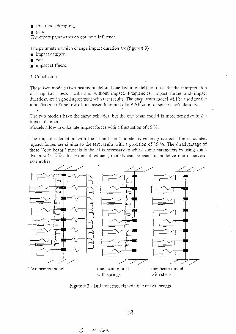
Three models are studied and compared to test results (figure #:3 ).

The first model is a two beams model. In this model, one beam represents -the fel rods andasecond one the uide-thimbles. Grids are modelled by masses and springs (Ki). Rotation

springs (Kcr) located between grids represent the grid-rod connections and springs Ktr

represent connections between guide-thimbles and grids. When the excitation level

increases. slippages which appear between rids and rods are taken into account by areduction coefficient applied on spnga values (Kcr).

This model has been validated by comparison with tests results on several scale one felassemblies, and on reduced scale mockups in air and in water.

The two other models consist in only one-bearn which represents guide-thimbles and fuelrods. The model has rotational springs similary to the 2 beams model. The last model doesnot have spring, but shear is taken into account.The table # 3 presents different hypothesis to calculated section, inertia and shearfor the onebeam model with shear. In a first step, the beam is embedded at each extremity. Inertia andsection of the beam are equal to the sumn of inertias and sections of all fuel rods and guide-thimbles. In this case, calculated frequencies are lower than measured frequencies.Ln a second step, inertia takes into account the position of each rod (Huygehens terms) Thereare no otation. Rods and uide-thimbles are considered as embedded in rids. Calculatedfrequenci-es are higher than measured ffequencies.i a last step, shear is taken into account with the same conditions as the first one beam

model. In this case. results are similar to those of the 2 beams model.

During tests, we have observed that springs, and dimples of the extremity grids ~were flabby.The decrease of the rotational springs atthe exremity on he fuel rd beam allost a7ivery good agreement between measured and calculated frequencies.With the one beam model, the decreasing, of the shear coefficient at the extremity of thebeam does not allow to find the measured frequencies. It is necessary to adjust inertia tohave a good agreement.

The table # 4 presents calculation results Using a model with one beam and springs. A firstcalculation is performed with. grid rotations equal to zero. Calculated-frequencies are higherthan measured frequencies. In ~L second step, grid rotations are free, but we insert rtationalsprings Kt. These springs are defined by the rotational stiffness values Kcr for rods and Ktufor guide-thimbles and are calculated by

with Kt = Kcr + Ktu and Kcr or Ktu = (ES/L)_z`E = Young modulus

S=section of rods or gridsL = distance between two grids-z = distance between rods or guide thimbles and the assembly axe

Frequencies are higher than measured frequencies, but they are equivalent to the calculatedfrequencies with the two beams model without adjustment of the springs at the extremitiesof the fuel rod beam. If we decrease the spring value at the extremities of the beam of thisone beam model, we obtain also a very good agreement with tests results like with the twobeams model.

To take into account the sliding of fuel rods in rids which decreases frequencies infuinction of the amplitude of excitation, we introduce a reduction coefficient on the springvalues. The coefficient is determined by comparison with tests results.

- k~~~~~~~~~~~~~5

Figure 4 shows the comparison of the static st iffness bteween test results and calculationsfor the 3models.

Figure A 5 shows the evolution of the maximum impact force in fulnction. of the snap backamplitude. We observe that all results are similar.

Figure R' 6 shows the evolution of the impact force integral in fuinction of the amplitude.Wehave very good agreement between test results and calculations performed with the onebeam model with shear.

3.3. Parametric studies

Some parameter sensitivities have been studied like:a firts mode damping,a impact damper,a impact stiffness,2 gaps.

Comparisons have been performed on snap back test results like:• the temporal response (displacement),• impact duration,-* integral of the impact forces.-

The first mode damping have effect on the 2 models. When the damping increases• the rebound decreases,• the impact duration is not modifie-d.

For the other dampings, the-one beam model is less sensitive than the 2 beams model.When_dampings increase, the maximum impact force does not change significantely. With the 2beam model, these parameters allow to have a very good ag1r.ement on the velocity signalduring the impact duration (same oscillations).

When we do not introduce impact damper, the impact force shows several peaks. When thedamper increases, the number of peaks decreases to only one peak. The damper value isadjusted by comparison between measured and calculated velocity during the impact.

When the gap increases the maximum force value, integral of forces and ipact durationdecrease.

Figures # 7 to --' 9 show the maximum impact force variation, integral force and durationvariations when different parameters fluctuate of ± 50%,/.

The most important parameters which modifie impact force are (figure 7):• impact stiffness,• first mode damping,• impact damper.

The most important parameters which modifie integral force are (figure H 8)

V. <Co's

* first mode damping,* gap.The others parametres do not have influence.

The parameters which change impact duration are (figure 9)z1 impact damper,m gap.u1 impact stiffes

4. Conclusion

These two models (two beams mi-odel and one beam model) are used for the interpretationof snap back tests with and without impact. Frequencies, impact forces and impactduratiosn are in good agreement with test results. The one beam modael wvill be used for the

modelisation of one row of fuel assemblies and of a P WR core for seismic calculations.

The two models have the samne behavior, but the one beam model is more sensitive to theimpact damper.1Models allow to calculate impact forces with a fluctuation of 1 5 %

The impact calculation-with the one beam'' model is generaly correct. The calculatedimnpact forces are similar to the test results wvith a precision of 15 %. The disadvantage ofthese ''one beam" models is that it is necessary to adjust some parameters in using somedyrramic tests results. After adjustment, models can be used to modelize one or severalassemblies.

Two beamns model one beam model one beam modelwith springs with shear

Figure #3-Different models with one or two beams

TABLE I - ONE.LEVEL FRANE

Corlfi1uratiol () Conllcuratioln (2) Conirailtioni (3) CoFrguratioun (') Configuraion (5) Confligurnfion (6)

CJ ~~~~Number '1I 1o f e le nie n ts _ _ _ _ _ _ _ _ _ _ _ _ _ _ _ _ _ _ _ _ _ _ _ _ _ _ _ _ _ _ _ _ _ _ _ _ _ _ _ _ _ _ _ _ _ _ _ _ _ _ _ _ _ _ _

Inertia 10=1. 594 1 0-1 n 10, = 1. 594 1010 m lo1 = 2 x 1.594 10-in 10 = x 1.594 1 0-T= 2 x 0 = x x 1 00

(iii4) in', Wil]4

Section S,= 1.5991 10-10 SO= 1.5991 10.10 S,=2x.5991 0-'~ S,=2x.5991 101)1 S., =2 x S S~r F X S,

(ni2 ) rn2 ?i?

Mass 0.639 0.639 0.639 0.639, 0.639 0.639

(kg) __ _ _ _ __ _ _ _

Em bedded EmbeddedB ou nda ry at the bottom E xSCR d d2 at tlie bottom E SCR X d2Sheat. Shearconditions Kry = L YL12 PIfx 2 x(1+y) 12 x -x 2 x ( +y)

1 10 ̀ N/m n Embedded ST- X 112 S- X it2

X R= ~~~10''N/rn at the bottom 1 .2441 1 0' 1.24, 10-'

Frequncies 1 7.63 17.59 11.08 17.59 9.47 17.58Frequncies 70.52 70.06 69.42 94.93 91.09

95.25 94.93

TABLE H 2 - FIVE LEVELS FRAIME

INumber 5-

Nu mbe r 64 6 263M

of elementst_ _ _ _ _ _ _ _ _ _ _ _ __ _ _ _ _ _ _ _ _ _ _

Heighit 5

Inertia =' 1.594' l0IJ mj2'<a 1 0 00 X I(

(m4)

-Section SO= 1.59 1 1 0-1u m2 1 S S T~x

v a Ss 6.0766 6.0766 6.07665

Boundary Embedded12ITx2 2< conditions at the bottomn Cis K 2< 1

<2x(+)2<E> SCR x d2

ST xIh LRj 0" N/r

0.38 0.857 0.356 0.37 0.372.67- -2.61 - 2.56 642.66

Frequencies 4. 52 4.49 4.31 4.51 4.58(Hz)

L _____ ____________ _____ L=2.5 ____________

TABLE H, XLI FUEL ASSEMBL31Y -

ONE BEAM MODEL- WITH SHEAR

R y

Number of grids 101 1 0 1 0 10

Nodes between grids 13Hleight (n) ___ _4.539 14.539 4.539 4.539

Ine1 -Ria5 ( 4) -T =-f E -M + CR 1, l;+ S 12 1000 1~ EII S d12

= 4. 829 1 m

Section ~~~~ S1. = ~~S~~f.G + ~T=9 .2 1 0 -+1.39 1 02) ST = 2sG + ESCR Sr Ys.G + C S.,. S.).S~(-

floundaiy =~~~~4.5876 1Wr 2 = 4.5876 1W=4.5876 Li 2=4.5876 103m

conditions Top and bottom Top01 and bottomCi :1- 2.(+)embedded embedlded Cis C2 I2 ± )

0.926 16..~3 '4.122.55 8.7 1 8.46

Frequencies 5.01 13.01 12.78

(Liz) ~~~~12 .4 ~ _ _ _ _ _ _ _ _ _ _ _ _ _ _ _ _

TABLE# L-XL FUEL ASSEMBLY-ONE BEAM MODEL WITH SPINGS

RYbioqlid

17277 ,7'7 T6 /77- 77-

Number of grids 1 0 1 0 1 0 1 0

-~~~~~~~~ ~~~Nodes behyeen grids 3 3 3 ' 3

A ~~~~~~~~~~~Height (in) 4.539 4.539 4.539 4.539

p... ~~~~Inertia (m') IT = E'TG + EICR

= 4.829 4- m

Scon(ini) ST = STG + SCR 1

S lb crilvolls ~~ ~~~~~ S c1raoils c .[],b l

Boundary iKCR L Zz KCR~ LR Z 2 K, R Yzcond itio us Li I.

S intbr lubes Kb li

4.44 4.11 3.74 3.48.9 8.62 8.B6.97

(Freqnces13.55 3.312.93 11.14(Liz) ~~~~~~~~~~~~18.16 1 7.98 17.50 15.30

Xl.E3 FORCE N)MAXII-1liH 1307.(N) ~~~~~~~~~~~~MINIMUM .00i0a .4 0 _ _ _ _

1. 2 0 -,

1. 00-

0 0~~~~~~~~I7

60~~~~~~~~~~~

BEAM M'OI)EL,

(Sh 1EA R)

2 1 AANIS N'OI ) EL1.20

1)iSPLACEMER11,NT (mil) TrEsTS.0 0 _ _ _ __ _ _ _ LI

.00 2 .00 4 .00 6. 00 8. 00 10. 00 12 .00 14.00 16.00 18. 00 2 0.00

STATIC STIFFNESS F igurc 4

IMPACT IN AIR AGAINST ONE R11) IMPACT N AIR AGAINST ONE GRIDMAXIMUM IMPACT FORCE INTEGRAL OlFTI-E M'ACT FORCE

6000--

50 0 0 - - - -- - -70-- - . . . . . . . . . . . . . . . . . . . . . . .

/ r I~ ~ ~~~~~~0. . . .. . .. . . . . .. . .

I cO~ ~ ~ ~ ~~~~~~........... ......

4000 -7 ------------------------- --

N I ~ ~ ~ ~ ~~~~~~~~~~~~~~~~~~~~~~~~ 5 o - - -- - - -. .. . ..-- -.-- - - -- -- - - - -- - - - - --- . . . .

'it-~~~~~~~~~~~~~~~~~~~~~~

I . . .~~~~~~~~~~~~~~~~~~~ .-- I /~0. . . . . . . . . . .. . . .1000 -- - - - - -- - - - - - - - - - - -- -I-- -

0 ~~~~~~~~~~~~~~~~~~~~~~~~~0

2.82 5.78 8.82 11.77 14.165 17.144 2 82 5 78 88?2 11.77 14 65 17.44Amplitude de lAcher (mmn) Arnplilude de IAchier (nm)

-u- TESTS -V- 2 BEAMS MODEI -W- TESTS - 2 111EAM.S MODEL

-- 1 BEAM MODEL 1I-I3EAM MODEL -G- 1 BEAM MODEL, 1 BEAM MODEL(SHEAR) - .(SPRINGS) . (SHEAR) (SPRINGS1Figure # 5 __________ -- . -Fi u e I 6

SIAXIRIUM IMPACT FORCE VARIATION IAIL'ACI'FOI(CI.'IN'I'b,'GltAl, VARIATION VARIATION

so 60

66

55 h)-54

SOG0so

V-V4500 50

40. 45ht

4000

4 6

4 03500

-1000 42

35-50 -30 -20 -10 0 10 20 30 40 50 ~50 -30 -20 -10 0 10 20 30 40 50 -50 -30 -210 -10 0 10 20 30 40 50PARARIETER VARIAVIONPARAMETER VMtRATI(N

-I- GAP DAMPING0F1110DES .2 -1 GAI, -Y- DASIPING0FbIODES �2 -1- G ke Y- DAMPING F-W. F111ST MODE DAMPING 0- ibli"tcl, L),%t.1PER Flit.ST6101)EA),kbli.E.N(;-[I]- IMPACTS1IFFNESS

Figur m 7 MAIPACrSTIFFNESS Figure 11 8

Figul c fl 9