DYNAMIC BEHAVIOR OF CONTINUOUS FLOW … BAP- 2001-07-02-02. I wish to thank Prof. Dr. Zeki Aktaş...
242
DYNAMIC BEHAVIOR OF CONTINUOUS FLOW STIRRED SLURRY REACTORS IN BORIC ACID PRODUCTION A THESIS SUBMITTED TO THE GRADUATE SCHOOL OF NATURAL AND APPLIED SCIENCES OF MIDDLE EAST TECHNICAL UNIVERSITY BY GAYE Ö. YÜCEL ÇAKAL IN PARTIAL FULFILLMENT OF THE REQUIREMENTS FOR THE DEGREE OF DOCTOR OF PHILOSOPHY IN THE DEPARTMENT OF CHEMICAL ENGINEERING JUNE 2004
Transcript of DYNAMIC BEHAVIOR OF CONTINUOUS FLOW … BAP- 2001-07-02-02. I wish to thank Prof. Dr. Zeki Aktaş...

DYNAMIC BEHAVIOR OF CONTINUOUS FLOW STIRRED SLURRY REACTORS IN BORIC ACID PRODUCTION
A THESIS SUBMITTED TO THE GRADUATE SCHOOL OF NATURAL AND APPLIED SCIENCES
OF MIDDLE EAST TECHNICAL UNIVERSITY
BY
GAYE Ö. YÜCEL ÇAKAL
IN PARTIAL FULFILLMENT OF THE REQUIREMENTS FOR THE DEGREE OF DOCTOR OF PHILOSOPHY
IN
THE DEPARTMENT OF CHEMICAL ENGINEERING
JUNE 2004

Approval of the Graduate School of Natural and Applied Sciences
Prof. Dr. Canan Özgen Director
I certify that this thesis satisfies all the requirements as a thesis for the degree of Doctor of Philosophy.
Prof. Dr. Timur Doğu Head of Department
This is to certify that we have read this thesis and that in our opinion it is fully adequate, in scope and quality, as a thesis and for the degree of Doctor of Philosophy.
Prof. Dr. İnci Eroğlu Supervisor
Examining Committee Members
Prof. Dr. Hayrettin Yücel (METU CHE)
Prof. Dr. İnci Eroğlu (METU CHE)
Prof. Dr. Saim Özkar (METU CHEM)
Prof. Dr. Nusret Bulutcu (ITU CHE)
Prof. Dr. Nurcan Baç (METU CHE)

I hereby declare that all information in this document has been
obtained and presented in accordance with academic rules and ethical
conduct. I also declare that, as required by these rules and conduct, I have
fully cited and referenced all material and results that are not original to
this work.
Name, Last name : Gaye Ö. Yücel Çakal
Signature :

iv
ABSTRACT
DYNAMIC BEHAVIOR OF CONTINUOUS FLOW STIRRED SLURRY REACTORS IN BORIC ACID PRODUCTION
Yücel Çakal, Gaye Ö.
Ph.D., Department of Chemical Engineering
Supervisor: Prof. Dr. İnci Eroğlu
June 2004, 213 pages
One of the most important boron minerals, colemanite is reacted with sulfuric acid
to produce boric acid. During this reaction, gypsum (calcium sulfate dihydrate) is
formed as a byproduct. In this study, the boric acid production was handled both in
a batch and four continuously stirred slurry reactors (4-CFSSR’s) in series system.
In this reaction system there are at least three phases, one liquid and two solid
phases (colemanite and gypsum). In a batch reactor all the phases have the same
operating time (residence time), whereas in a continuous reactor all the phases
may have different residence time distributions. The residence time of both the
reactant and the product solids are very important because they affect the
dissolution conversion of colemanite and the growth of gypsum crystals.

v
The main aim of this study was to investigate the dynamic behavior of continuous
flow stirred slurry reactors. By obtaining the residence time distribution of the solid
and liquid components, the non-idealities in the reactors can be found. The
experiments performed in the continuous flow stirred slurry reactors showed that
the reactors to be used during the boric acid production experiments approached
an ideal CSTR in the range of the stirring rate (500-750 rpm) studied.
The steady state performance of the continuous flow stirred slurry reactors
(CFSSR’s) in series was also studied. During the studies, two colemanites having
the same origin but different compositions and particle sizes were used.
The boric acid production reaction consists of two simultaneous reactions,
dissolution of colemanite and crystallization of gypsum. The dissolution of
colemanite and the gypsum formation was followed from the boric acid and calcium
ion concentrations, respectively. The effect of initial CaO/ SO42- molar ratio (1.00,
1.37 and 2.17) on the boric acid and calcium ion concentrations were searched.
Also, at these initial molar ratios the colemanite feed rate was varied (5, 7.5, 10 and
15 g/min) to change the residence time of the slurry.
Purity of the boric acid solution was examined in terms of the selected impurities,
which were the magnesium and sulfate ion concentrations. The concentrations of
them were compared at the initial molar ratios of 1.00 and 1.37 with varying
colemanite feed rates. It was seen that at high initial CaO/ SO42- molar ratios the
sulfate and magnesium ion concentrations decreased but the calcium ion
concentration increased.
The gypsum crystals formed in the reaction are in the shape of thin needles. These
crystals, mixed with the insolubles coming from the mineral, are removed from the
boric acid slurry by filtration. Filtration of gypsum crystals has an important role in
boric acid production reaction because it affects the efficiency, purity and
crystallization of boric acid. These crystals must grow to an appropriate size in the

vi
reactor. The growth process of gypsum crystals should be synchronized with the
dissolution reaction.
The effect of solid hold-up (0.04–0.09), defined as the volume of solid to the total
volume, on the residence time of gypsum crystals was investigated and the change
of the residence time (17-60 min) on the growth of the gypsum was searched. The
residence time at each reactor was kept constant in each experiment as the
volumes of the reactors were equal. The growth of gypsum was examined by a
laser diffraction particle size analyzer and the volume weighted mean diameters of
the gypsum crystals were obtained. The views of the crystals were taken under a
light microscope. It was observed that the high residence time had a positive effect
on the growth of gypsum crystals. The crystals had volume weighted mean
diameters of even 240 µm.
The gypsum crystal growth model was obtained by using the second order
crystallization reaction rate equation. The residence time of the continuous reactors
are used together with the gypsum growth model to simulate the continuous boric
acid reactors with macrofluid and microfluid models. The selected residence times
(20-240 min) were modeled for different number of CSTR’s (1-8) and the PFR.
The simulated models were, then verified with the experimental data. The
experimentally found calcium ion concentrations checked with the concentrations
found from the microfluid model. It was also calculated that the experimental data
fitted the microfluid model with a deviation of 4-7%.
Key words: Gypsum Crystallization, Boric Acid, Colemanite Dissolution, Slurry
Reactors, Residence Time Distribution, Macrofluid Model, Microfluid
Model

vii
ÖZ
BORİK ASİT ÜRETİMİNDE KULLANILAN SÜREKLİ AKIŞLI KARIŞTIRMALI ÇAMUR REAKTÖRLERİNİN DİNAMİK DAVRANIŞI
Yücel Çakal, Gaye Ö.
Doktora, Kimya Mühendisliği Bölümü
Tez Yöneticisi: Prof. Dr. İnci Eroğlu
Haziran 2004, 213 sayfa
Önemli bor minerallerinden biri olan kolemanitin, sülfürik asit ile reaksiyona girmesi
sonucunda borik asit üretilmektedir. Bu reaksiyon esnasında jips (kasiyum sülfat
dihidrat) yan ürün olarak oluşmaktadır. Bu çalışmada, borik asit üretimi hem kesikli
hem de dörtlü seri bağlantılı sürekli akışlı karıştırmalı çamur reaktörleri sisteminde
ele alınmıştır.
Bu reaksiyon sisteminde en az üç tane faz vardır, bir sıvı ve iki katı faz (kolemanit
ve jips). Kesikli reaktörde bütün fazlar aynı işetme zamanına (reaktörde kalış
süresine) sahiptir. Bunun yanısıra, sürekli reaktörde hem reksiyona giren katının
hem de ürün olan katının reaktörde kalış süresi çok önemlidir çünkü bu kolemanitin
çözünme dönüşümünü ve de jips kristallerinin büyümesini etkilemektedir.

viii
Bu çalışmanın esas amacı, sürekli akışlı karıştırmalı çamur reaktörlerinin dinamik
davranışını incelenmektir. Katı ve sıvı bileşenlerin reaktörde kalış süresini elde
ederek, reaktördeki ideal olmayan koşullar saptanabilmektedir. Sürekli akışlı
karıştırmalı çamur reaktörlerinde yapılan çalışmalar borik asit üretimi deneylerinde
kullanılan reaktörlerin çalışılan karıştırma hızlarında (500-750 rpm) ideal karıştımalı
tank reaktörlerine yaklaştığını göstermektedir.
Seri bağlantılı sürekli akışlı karıştırmalı çamur reaktörlerinin yatışkınhal performansı
da çalışılmıştır. Bu çalışmalar esnasında, aynı yerden gelen fakat farklı
kompozisyonlara ve parça boyutuna sahip iki kolemanit kullanılmıştır.
Borik asit üretim reaksiyonu iki birbirini takip eden reaksiyondan oluşmaktadır,
kolemanitin çözünmesi ve jipsin kristalizasyonu. Kolemanit çözünmesi ve jips
oluşumu, sırasıyla, borik asit ve kalsiyum iyon konsantrasyonu ile takip
edilmektedir. Başlangıç CaO/ SO42- mol oranının (1.00, 1.37 ve 2.17) borik asit ve
kalsiyum iyon konsantrasyonuna etkisi araştırılmıştır. Bu başlangıç mol oranlarında,
çamurun reaktörde kalış süresini değiştirmek için farklı kolemanit besleme hızları
(5, 7.5, 10 ve 15 g/dak) kullanılmıştır.
Borik asit çözeltisinin saflığı, seçilen safsızlıklar, magnezyum ve sülfat iyonları
konsantrasyonları, ile incelenmiştir. Bu konsantrasyonlar, başlangıç mol oranı 1.00
ve 1.37 olduğu durumlarda, kolemanit besleme hızlarını değiştirerek
karşılaştırılmıştır. Yüksek başlangıç CaO/ SO42- mol oranınında sülfat ve
magnezyum iyon konsantrasyonlarının azaldığı fakat kalsiyum iyon
konsantrasyonunun arttığı görülmüştür.
Reaksiyonda oluşan jips kristalleri ince iğneler şeklindedir. Bu kristaller, mineralden
gelen çözünmemişlerle karışıp, borik asit çamurundan filtrasyonla uzaklaştırılır. Jips
kristallerinin filtrasyonunun borik asit üretim reaksiyonunda önemli bir yeri vardır
çünkü bu işlem, verimi, saflığı ve borik asidin kristalizasyonunu etkilemektedir. Bu
kristaller reaktörde uygun bir boyuta büyütülmek zorundadır. Jips kristallerinin
büyüme prosesi çözünme reaksiyonu ile senkronize bir şekilde çalışmalıdır.
Katı tutma oranının (0.04-0.09) jips kristallerinin reaktörde kalış süresine etkisi
araştırılmış ve reaktörde kalış süresi değişimi (17-60 min) ile jipsin büyümesi

ix
incelenmiştir. Katı tutma oranı, katı hacminin toplam hacime oranı şeklinde ifade
edilir. Deneyler esnasında, her reaktördeki kalış süresi, reaktörlerin hacmi eşit
olduğundan sabit kalmıştır. Jips büyümesi lazer krınım parça boyut analiz cihazı ile
incelenmiş ve jips kristallerinin hacimce ortalama çapları elde edilmiştir. Kristal
görüntüleri ışık mikroskobu ile çekilmiştir. Yüksek reaktörde kalış süresinin jips
kristal büyümesine positif bir etkisi olduğu gözlemlenmiştir. Kristallerin hacimce
ortalama çapları 240 µm’a kadar varmıştır.
Jips kristal büyüme modeli, ikinci dereceden kristalizasyon reaksiyonu hız denklemi
ile elde edilmiştir. Sürekli borik asit reaktörlerinin makroakışkan ve mikroakışkan
modeli ile simulasyonu için, sürekli reaktörlerdeki reaktördeki kalış süresi jips
büyüme modeli ile birlikte kullanılmıştır. Değişik sayıdaki sürekli karıştırmalı tank
reaktörleri (1-8) ve piston akış reaktörler, seçilen reaktörde kalış süreleri (20-240
dak) ile modellenmiştir.
Simule edilen modeller, daha sonra deneysel veri ile doğrulanmıştır. Deneysel
olarak bulunan kalsiyum iyon konsantrasyonları mikroakışkan modeli ile bulunan
konsantrasyonlarla uymuştur. Deneysel verinin mikroakışkan modelinden % 4-7
oranında saptığı bulunmuştur.
Anahtar Kelimeler: Jips Kristalizasyonu , Borik Asit, Kolemanit Çözünmesi, Çamur
Reaktörleri, Kalış Süresi Dağılımı, Makroakışkan Modeli,
Mikroakışkan Modeli

x
ACKNOWLEDGMENTS
It is a great pleasure for me to have the opportunity to express my deepest gratitude
to my supervisor Prof. Dr. İnci Eroğlu for her invaluable supervision, continuous
support and helpful suggestions throughout the course of this investigation.
I also wish to express my gratitude to my examining committee members Prof. Dr.
Saim Özkar and Prof. Dr. Hayrettin Yücel for their encouragement and comments
during the course of the study.
Special thanks are due to Prof. Dr. Nusret Bulutcu and Funda Altun for the valuable
discussions and advise.
I would like to thank Eti Maden İşletmeleri for the colemanite, sulfuric acid and boric
acid supports and METU for the financial support with the BAP Project with the
number BAP- 2001-07-02-02.
I wish to thank Prof. Dr. Zeki Aktaş for giving us time for the particle size analysis
and letting us use the analyzer. I also would like to thank Kerime Güney for the
chemical analysis, and all the Ch.E. Workshop members for their continuous help
throughout the thesis.
I would like to express my sincere gratitude to my friends Anıl Erdoğdu, Deniz
Gürhan and Işık Aşar for their helps during the continuous boric acid production
experiments and Salih Obut for the Mat Lab Programming. I also would like to thank
my room mates Barış Ünal and Ceren Oktar for the valuable discussions and
listening to me whenever I need.
Furthermore, I would like to express my deepest gratefulness to my family. Without
their support, tolerance and encouragement, this thesis could not have come to an
end.
Finally, I am thankful to my husband for his understanding and unlimited support.

xi
To My Dearest Husband Teoman
and Beloved Son Emre ...

xii
TABLE OF CONTENTS
Page ABSTRACT ...................................................................................................... iv
ÖZ ..................................................................................................................... vii
ACKNOWLEDGEMENT ................................................................................... x
TABLE OF CONTENTS ................................................................................... xii
LIST OF TABLES ............................................................................................. xvii
LIST OF FIGURES ........................................................................................... xxii
LIST OF SYMBOLS AND ABBREVIATIONS .................................................. xxviii
CHAPTER
1. INTRODUCTION .................................................................................... 1
1.1. Borate Minerals .............................................................................. 1
1.2. Boric Acid Production in the World ................................................ 4
1.3. Boric Acid Production in Turkey ..................................................... 6
2. LITERATURE SURVEY ......................................................................... 10
2.1. Dissolution of Colemanite and Its Kinetics .................................... 10
2.2. Crystal Growth of Calcium Sulfate Dihydrate and Its Kinetics ...... 12 2.3. Heterogeneous Solid Fluid Reaction Modeling .............................. 15
2.4. The Studies On The Residence Time Distribution In Fluid-Solid Reactors......................................................................................... 18
2.5. Reactor Modeling with Residence Time Distribution...................... 20
2.6. Objective of the Present Study....................................................... 21
3. MODELING ............................................................................................ 23
3.1. Gypsum Crystal Growth Model ...................................................... 24

xiii
3.2. Terminology of Mixing .................................................................... 24
3.3. Simulation of Continuous Flow Reactors ....................................... 27
3.3.1. Macrofluid Model for n-CSTR’s in Series .............................. 28
3.2.2. Microfluid Model for n-CSTR’s in Series ............................... 31
3.3.3. Plug Flow Model ................................................................... 32
4. EXPERIMENTAL .................................................................................... 34
4.1. Materials ........................................................................................ 34
4.2. Batch Reactor Experiments ........................................................... 34
4.2.1. Experimental Setup ............................................................... 34
4.2.2. Experimental Procedure ....................................................... 37
4.2.3. Scope of the Experiments ..................................................... 37
4.3. Continuous Flow Stirred Slurry Reactors in Series Experiments.... 37
4.3.1. Experimental Setup ............................................................... 38
4.3.2. Dynamic Behavior Experiments ............................................ 43
4.3.2.1. Experimental Procedure ............................................ 43
4.3.2.2. Scope of the Experiments ......................................... 44
4.3.3. Boric Acid Production Experiments ....................................... 45
4.3.3.1. Experimental Procedure ............................................ 45
4.3.3.2. Scope of the Experiments ......................................... 46
4.4. Analytical Procedures .................................................................... 49
4.4.1. Determination of Boric Acid Concentration ........................... 49
4.4.2. Determination of Calcium Ion Concentration ........................ 49
4.4.3. Determination of Sulfate Ion Concentration .......................... 49
4.4.4. Determination of Magnesium Ion Concentration ................... 50
4.4.5. Crystal Size Determination ................................................... 50
4.4.5.1. Particle Size Distribution of Gypsum Crystals ........... 50
4.4.5.2. Light Microscope Images of Gypsum Crystals .......... 51

xiv
5. RESULTS AND DISCUSSION ............................................................... 52
5.1. Results of Colemanite Analysis ..................................................... 52
5.1.1. Screen Analysis of Colemanite ............................................. 52
5.1.2. Chemical Analysis of Colemanite ......................................... 57
5.1.3. Particle Size Distribution of Colemanite ................................ 59
5.2. Dynamic Behavior Experiments on Continuous Flow Stirred Slurry Reactors .............................................................................. 61
5.2.1. Liquid Residence Time Experiments .................................... 62
5.2.1.1. Effect of Stirring Rate on Liquid Residence Time ..... 62
5.2.1.2. Check of Different Tracers on Liquid Residence Time ........................................................................... 66
5.2.2. Solid Residence Time Experiments ...................................... 69
5.2.3. Liquid Residence Time Experiments in a Solid/Liquid System .................................................................................. 71
5.2.3.1. Effect of Stirring Rate on Liquid Residence Time ..... 71
5.2.3.2. Effect of Solid to Liquid Ratio on Liquid Residence Time .......................................................................... 73
5.3. Batch Reactor Experiments ........................................................... 78
5.4. Boric Acid Production Experiments on Continuous Flow Stirred Slurry Reactors in Series ............................................................... 83
5.4.1. Parameters Affecting the Performance of CFSSR’s in Series .................................................................................... 84
5.4.2. Variation of the Concentration of Boric Acid in Solution at Steady State ......................................................................... 84
5.4.3. Variation of the Concentration of Calcium Ion in Solution at Steady State ......................................................................... 88
5.4.4. pH and Temperature Variation of the Experiments at Steady State ......................................................................... 93
5.4.5. Variation of the Concentrations of Sulfate and Magnesium Ions in Solution at Steady State ............................................ 95
5.4.6. Comparison of Variation of Calcium and Sulfate Ion Molar Flow Rate .............................................................................. 97
5.4.7. Conversion Expressions Used During the Study .................. 98
5.4.8. Effect of Solid Hold-Up on the Residence Time of Liquid and Solid Components ......................................................... 99
5.5. Particle Size Distribution of Gypsum Crystals ................................ 101
5.5.1. Particle Size Distribution of Gypsum Crystals in a Batch Reactor ................................................................................. 101
5.5.2. Particle Size Distribution of Gypsum Crystals in 102

xv
Continuous Flow Stirred Slurry Reactors ............................. 5.6. Light Microscope Images of Gypsum Crystals ............................... 112
5.6.1. Light Microscope Images of Gypsum Crystals in a Batch Reactor ................................................................................. 113
5.6.2. Light Microscope Images of Gypsum Crystals in Continuous Flow Stirred Slurry Reactors .............................. 113
5.7. Simulation of Boric Acid Reactors .................................................. 116
5.7.1. Gypsum Crystal Growth Model ............................................. 116
5.7.2. Simulation of Continuous Reactors ...................................... 122
5.7.2.1. Macrofluid model for n-CSTR’s in Series .................. 122
5.7.2.2. Mıcrofluid model for n-CSTR’s in Series ................... 126
5.7.2.3. Plug Flow Model ........................................................ 130
5.7.2.4. Comparison of the Model Results ............................. 133
5.8. Comparison of the Results ............................................................. 136
5.8.1. Batch Reactor versus Continuous Reactor Experiments ..... 136
5.8.2. Verification of the Experimental Data with the Model Results ................................................................................. 140
6. CONCLUSIONS ..................................................................................... 143
7. RECOMMENDATIONS........................................................................... 147
REFERENCES ................................................................................................. 149
APPENDICES
A. Chemical Analysis of Colemanite ........................................................... 155
A.1. Determination of B2O3 Content ....................................................... 155
A.2. Determination of SiO2 Content ....................................................... 156
A.3. Determination of Na2O and K2O Content 157
A.4. Determination of CaO, MgO, Al2O3, Fe2O3, SrO and TiO2 Content ........................................................................................... 157
B. Raw Data of Dynamic Behavior Experiments ........................................ 158
B.1. Data of Liquid Residence Time Experiments ................................. 159
B.2. Data of Solid Residence Time Experiments ................................... 163
B.3. Data of Liquid Residence Time Experiments in a Solid / Liquid System ............................................................................................ 164

xvi
C. Raw Data of the Batch Reactor Experiments ......................................... 167
C.1. Data of Experiment HB2.1& HB2.2 ................................................ 168
C.2. Data of Experiment HB2.3 .............................................................. 170
C.3. Data of Experiment HB3.1 .............................................................. 171
D. Raw Data of Boric Acid Production Experiments in Continuously Stirred Slurry Reactors .......................................................................... 172
D.1. Data of Experiment HC2.1 ............................................................. 173
D.2. Data of Experiment HC2.2 ............................................................. 175
D.3. Data of Experiment HC2.3 ............................................................. 177
D.4. Data of Experiment HC2.4 ............................................................. 179
D.5. Data of Experiment HC2.5 ............................................................. 182
D.6. Data of Experiment HC2.6 ............................................................. 184
D.7. Data of Experiment HC2.7 ............................................................. 186
D.8. Data of Experiment HC2.8 ............................................................. 188
D.9. Data of Experiment HC3.1 ............................................................. 190
D.10. Data of Experiment HC3.2 ........................................................... 192
E. Raw Data of Solid Hold-up Experiments ................................................ 194
F. Sample Calculations ............................................................................... 197
F.1. CaO/SO42- Molar Ratio Calculation ................................................. 198
F.2. Solid Hold-up, Calculation .............................................................. 199
F.3. Residence Time of Solid and Liquid Components in the Reactor .. 199
F.4. Material Balances ........................................................................... 201
F.5. Conversion Calculations ................................................................. 202
F.6. Unit Conversions ............................................................................ 203
G. Modeling ................................................................................................ 205
G.1. Macrofluid Model Mat Lab Program ............................................... 206
G.2. Microfluid Model Mat Lab Program ................................................ 207
G.3. Mat Lab Program Outputs for the Verification of Experimental Data ................................................................................................ 208
VITA .................................................................................................................. 213

xvii
LIST OF TABLES
TABLE Page
1.1. Commercially important borate minerals (Roskill, 2002) ..................... 2
1.2. Distribution of borate minerals (Kirk Othmer, 1992) ............................ 3
1.3. Reserves of boron minerals in Turkey (Roskill, 2002) ........................ 3
1.4. Boric acid producers and their capacities (Roskill, 2002).................... 5
3.1. Comparison of macrofluid and microfluid behavior in a reactor ......... 27
3.2. Comparison of batch, plug flow and mixed flow reactors in terms of the behaviors of micro and macrofluids .............................................. 27
4.1. The Batch Reactor Experiments Performed during the Study ............ 37
4.2. Dynamic Behavior Experiments Performed .............................. ......... 44
4.3a. Performed Experiments in Grouped Style in Continuous Flow Stirred Slurry Reactors in Series .................................................................... 47
4.3b. Performed Experiments in Continuous Flow Stirred Slurry Reactors in Series ............................................................................ ................. 48
5.1.1. The screen analysis of Hisarcık 1 colemanite ..................................... 53
5.1.2. The screen analysis of Hisarcık 2 colemanite ..................................... 54
5.1.3. The screen analysis of Hisarcık 3 colemanite ..................................... 56
5.1.4. Chemical analysis of Hisarcık 1 colemanite (dry basis, wt%) (METU, Chemical Eng. Dept.) .......................................................................... 58
5.1.5. Chemical analysis of Hisarcık colemanites (dry basis, wt%) (METU, Chemical Eng. Dept.) .......................................................................... 59
5.1.6. Volume weighted mean diameters of the colemanites ....................... 61
5.2.1. Comparison of the two experimental values with the theoretical ones (volumetric flow rate = 42.5 ml/min, tracer= nickel) ............................. 66
5.2.2. Comparison of different tracers with the theoretical ones (volumetric slow rate = 42.5 ml/min, stirring rate = 500 rpm) ................................. 68
5.2.3. Comparison of the residence time and the variance per square of residence time for step input experiments .......................................... 70
5.2.4. Comparison of the residence time of liquid and solid and the variance per square of liquid residence time for different stirring rates .............. 72

xviii
5.2.5. Comparison of the residence time of liquid and the variance per square of residence time for different solid to liquid ratios (g solid/ml liquid) ................................................................................................... 74
5.2.6. The residence time of liquid evaluated from Figure 5.2.11 and Equation 5.2.17 at different solid to liquid ratios (g solid/ml liquid) ….. 76
5.4.1. Steady state values of produced boric acid concentrations and molar flow rates in the experiments .............................................................. 84
5.4.2. Steady state values of calcium ion concentrations and molar flow rates in the experiments ...................................................................... 88
5.4.3. Steady state values of pH and temperature in the experiments ......... 93
5.4.4. Steady state values of the magnesium and sulfate ion concentrations in the fourth reactor in the experiments ............................................... 94
5.4.5. Conversion calculated in terms of colemanite and sulfate ion entering the system ........................................................................................... 98
5.4.6. Solid hold-up and residence time of the solid and liquid components in each of the reactors in series .......................................................... 99
5.5.1. Volume weighted mean diameter (µm) of the particles obtained from the software of the laser diffraction particle size analyzer for the experiments performed by using Hisarcık 2 colemanite, 0-250 µm .... 108
5.7.1. The model parameters of the batch reactor experiments ................... 119
5.7.2. Gypsum Crystal Growth Model Obtained from Different Batch Reactor Experiments ........................................................................... 120
5.7.3. The calcium ion concentration evaluated at the exit of the nth CSTR, estimated by macrofluid model using the rate expression in Eq. 5.7.1 (Co = 0.053 mol/l, Csat = 0.013 mol/l) ................................................... 123
5.7.4. The calcium ion concentration evaluated at the exit of the nth CSTR, estimated by macrofluid model using the rate expression in Eq. 5.7.2 (Co = 0.043 mol/l, Csat = 0.011 mol/l) ................................................... 124
5.7.5. The calcium ion concentration evaluated at the exit of the nth CSTR, estimated by macrofluid model using the rate expression in Eq. 5.7.3 (Co = 0.0299 mol/l, Csat = 0.0056 mol/l) ............................................... 124
5.7.6. The calcium ion concentration evaluated at the exit of the nth CSTR, estimated by microfluid model using the rate expression in Eq. 5.7.1 (Co = 0.053 mol/l, Csat = 0.013 mol/l) ................................................... 127
5.7.7. The calcium ion concentration evaluated at the exit of the nth CSTR, estimated by microfluid model using the rate expression in Eq. 5.7.2 (Co = 0.043 mol/l, Csat = 0.011 mol/l) ................................................... 127
5.7.8. The calcium ion concentration evaluated at the exit of the nth CSTR, estimated by microfluid model using the rate expression in Eq. 5.7.3 (Co = 0.0299 mol/l, Csat = 0.0056 mol/l) ............................................... 128
5.7.9. Plug Flow Model Expressions ............................................................. 131
5.7.10. The calcium ion concentration evaluated at the exit of the PFR with the plug flow models given in Table 5.7.9 ........................................... 132

xix
5.8.1. Comparison of batch reactor and continuous reactor results performed by Hisarcık 2, 0-250 µm, colemanite in terms of boric acid, calcium ion concentrations, pH and volume weighted mean diameter (µm) of the gypsum crystals obtained at initial CaO/SO4
2-molar ratio of 1.00, Stirring Rate = 500 rpm (batch), 400 rpm (continuous), temperature = 85°C ............................................................................. 138
5.8.2. Comparison of batch reactor and continuous reactor results performed by Hisarcık 3, 0-150 µm, colemanite in terms of boric acid, calcium ion concentrations, pH and volume weighted mean diameter (µm) of the gypsum crystals obtained at initial CaO/SO4
2-molar ratio of 1.00, stirring rate =400 rpm, temperature = 85°C ............................ 139
5.8.3. Calcium ion concentrations at the exit of the CSTR’s obtained by macrofluid, microfluid models and the experimental data ................... 141
B.1. Variation in nickel concentrations in liquid residence time experiments at different stirring rates .................................................. 159
B.2. Comparison of E(t) and F(t) values of the liquid residence time experiments and the ideal reactor (Pulse tracer=Nickel) .................... 160
B.3. Variation in the concentrations of different tracers on the liquid residence time at 500 rpm ................................................................... 161
B.4. Comparison of E(t) and F(t) values of different tracers (stirring rate=500 rpm) and the ideal reactor .................................................... 162
B.5. Variation in colemanite weight during positive and negative step tracer experiments (Stirring Rate=500 rpm) ........................................ 163
B.6. Variation in nickel concentrations in liquid residence time experiments at different stirring rates .................................................. 164
B.7. Variation in lithium concentrations of liquid at different solid to liquid ratios (g solid/ml liquid) ....................................................................... 165
B.8. The -ln (C/C0) vs t/τ values for different S/L ratios (g solid/ml liquid).................................................................................................... 166
C.1. Boric acid and calcium ion concentrations during the Experiment HB2.1, Hisarcık 2 colemanite, 0-250 µm, CaO/SO4
2- = 0.95, stirring rate = 500 rpm, T= 80°C ..................................................................... 168
C.2. Boric acid and calcium ion concentrations during the Experiment HB2.2, Hisarcık 2 colemanite, 250-1000 µm, CaO/SO4
2- = 0.95, stirring rate = 500 rpm, T= 80°C ......................................................... 169
C.3. Boric acid and calcium ion concentrations during the Experiment HB2.3, Hisarcık 2 colemanite, 0-250 µm, CaO/SO4
2- = 1, stirring rate = 500 rpm, T= 85°C ............................................................................ 170
C.4. Variation in pH during the Experiment HB2.3, Hisarcık 2 colemanite, 0-250 µm, CaO/SO4
2- = 1, stirring rate = 500 rpm, T= 85°C ............... 170
C.5. Boric acid and calcium ion concentrations during the Experiment HB3.1, Hisarcık 3 colemanite, 0-150 µm, CaO/SO4
2- = 1, stirring rate = 400 rpm, T= 85°C ............................................................................ 171
C.6. Variation in pH during the Experiment HB3.1, Hisarcık 3 colemanite, 0-150 µm, CaO/SO4
2- = 1, stirring rate = 400 rpm, T= 85°C ............... 171

xx
D.1. Calcium ion concentrations of the effluent streams during the Experiment HC2.1, Hisarcık 2 colemanite, 0-250 µm, CaO/SO4
2- = 1, stirring rate = 400 rpm, T= 85°C, colemanite feed rate = 5 g/min ........ 173
D.2. Temperature and pH values during the Experiment HC2.1, Hisarcık 2 colemanite, 0-250 µm, CaO/SO4
2- = 1, stirring rate = 400 rpm, T= 85°C, colemanite feed rate = 5 g/min .................................................. 174
D.3. Calcium ion concentrations of the effluent streams during the Experiment HC2.2, Hisarcık 2 colemanite, 0-250 µm, CaO/SO4
2- = 1, stirring rate = 400 rpm, T= 85°C, colemanite feed rate = 7.5 g/min ..... 175
D.4. Temperature and pH values during the Experiment HC2.2, Hisarcık 2 colemanite, 0-250 µm, CaO/SO4
2- = 1, stirring rate = 400 rpm, T= 85°C, colemanite feed rate = 7.5 g/min ............................................... 176
D.5. calcium ion concentrations of the effluent streams during the Experiment HC2.3, Hisarcık 2 colemanite, 0-250 µm, CaO/SO4
2- = 1, stirring rate = 400 rpm, T= 85°C, colemanite feed rate = 10 g/min ...... 177
D.6. Temperature and pH values during the Experiment HC2.3, Hisarcık 2 colemanite, 0-250 µm, CaO/SO4
2- = 1, stirring rate = 400 rpm, T= 85°C, colemanite feed rate = 10 g/min ................................................ 178
D.7. Calcium ion concentrations of the effluent streams during the Experiment HC2.4, Hisarcık 2 colemanite, 0-250 µm, CaO/SO4
2- = 1.37, stirring rate = 400 rpm, T= 85°C, colemanite feed rate = 5 g/min..................................................................................................... 179
D.8. Temperature and pH values during the Experiment HC2.4, Hisarcık 2 colemanite, 0-250 µm, CaO/SO4
2- = 1.37, stirring rate = 400 rpm, T= 85°C, colemanite feed rate = 5 g/min .................................................. 180
D.9. Calcium ion concentrations of the effluent streams during the Experiment HC2.5, Hisarcık 2 colemanite, 0-250 µm, CaO/SO4
2- = 1.37, stirring rate = 400 rpm, T= 85°C, colemanite feed rate = 10 g/min .................................................................................................... 182
D.10. Temperature and pH values during the Experiment HC2.5, Hisarcık 2 colemanite, 0-250 µm, CaO/SO4
2- = 1.37, stirring rate = 400 rpm, T= 85°C, colemanite feed rate = 10 g/min ................................................ 183
D.11. Boric acid and calcium ion concentrations of the effluent streams during the Experiment HC2.6, Hisarcık 2 colemanite, 0-250 µm, CaO/SO4
2- = 1.37, stirring rate = 400 rpm, T= 85°C, colemanite feed rate = 10 g/min .................................................................................... 184
D.12. Temperature and pH values during the Experiment HC2.6, Hisarcık 2 colemanite, 0-250 µm, CaO/SO4
2- = 1.37, stirring rate = 400 rpm, T= 85°C, colemanite feed rate = 10 g/min ................................................ 185
D.13. Calcium ion concentrations of the effluent streams during the Experiment HC2.7, Hisarcık 2 colemanite, 0-250 µm, CaO/SO4
2- = 1.37, stirring rate = 400 rpm, T= 85°C, colemanite feed rate = 15 g/min .................................................................................................... 186
D.14. Temperature and pH values of the effluent streams during the Experiment HC2.7, Hisarcık 2 colemanite, 0-250 µm, CaO/SO4
2- = 1.37, stirring rate = 400 rpm, T= 85°C, colemanite feed rate = 15 g/min ................................................................................................... 187

xxi
D.15. Calcium ion concentrations of the effluent streams during the Experiment HC2.8, Hisarcık 2 colemanite, 0-250 µm, CaO/SO4
2- = 2.17, stirring rate = 400 rpm, T= 85°C, colemanite feed rate = 10 g/min .................................................................................................... 188
D.16. Temperature and pH values during the Experiment HC2.8, Hisarcık 2 colemanite, 0-250 µm, CaO/SO4
2- = 2.17, stirring rate = 400 rpm, T= 85°C, colemanite feed rate = 10 g/min ................................................ 189
D.17. Boric acid and calcium ion concentrations of the effluent streams during the Experiment HC3.1, Hisarcık 3 colemanite, 0-150 µm, CaO/SO4
2- = 1.00, stirring rate = 400 rpm, T= 85°C, colemanite feed rate = 3.5 g/min ................................................................................... 190
D.18. Temperature and pH values during the Experiment HC3.1, Hisarcık 3 colemanite, 0-150 µm, CaO/SO4
2- = 1.00, stirring rate = 400 rpm, T= 85°C, colemanite feed rate = 3.5 g/min ............................................... 191
D.19. Boric acid and calcium ion concentrations of the effluent streams during the Experiment HC3.2, Hisarcık 3 colemanite, 0-150 µm, CaO/SO4
2- = 1.00, stirring rate = 400 rpm, T= 85°C, colemanite feed rate = 10 g/min..................................................................................... 192
D.20. Temperature and pH values during the Experiment HC3.2, Hisarcık 3 colemanite, 0-150 µm, CaO/SO4
2- = 1.00, stirring rate = 400 rpm, T= 85°C, colemanite feed rate = 10 g/min ................................................ 193
E.1. Variation of solid hold-up during the Experiment HC3.1, Hisarcık 3 colemanite, 0-150 µm, CaO/SO4
2- = 1.00, colemanite feed rate = 3.5 g/min ................................................................................................... 195
E.2. Variation of solid hold-up during the Experiment HC3.2, Hisarcık 3 colemanite, 0-150 µm, CaO/SO4
2- = 1.00, colemanite feed rate = 10 g/min ................................................................................................... 196
G.1. Output of Mat Lab Program for microfluid model for the verification of Experiment HC3.1 .............................................................................. 208
G.2. Output of Mat Lab Program for microfluid model for the verification of Experiment HC3.2 ............................................................................... 209
G.3. Output of Mat Lab Program for macrofluid model for the verification of Experiment HC3.1 ........................................................................... 211
G.4. Output of Mat Lab Program for macrofluid model for the verification of Experiment HC3.2 ........................................................................... 212

xxii
LIST OF FIGURES
FIGURE Page
2.1. Macrokinetics of heterogeneous solid-liquid reaction crystallizations (Bechtloff, 2001) .................................................................................. 16
2.2. Mechanism for sink type microphase .................................................. 18
3.1. Schematic representation of macrofluid behavior ............................... 26
3.2. Schematic representation of microfluid behavior ................................. 26
3.3. Schematic representation of inlet of the reactor, in which a microfluid or a macrofluid is entering the reactor ................................................. 26
3.4. Change of E(t) function with CSTR number ........................................ 30
3.5. Change of F(t) function with CSTR number ........................................ 30
4.1. Schematic diagram of the set-up used for the batch reactor experiments ......................................................................................... 35
4.2. Photograph of the set-up used for the batch reactor experiments … 36
4.3. Schematic diagram of the set-up used for the continuous flow stirred slurry reactor experiments ................................................................... 40
4.4. Technical drawing of the continuous flow stirred slurry reactor ……… 41
4.5. Photograph of the set-up used for the continuous flow stirred slurry reactor experiments ............................................................................. 42
5.1.1. Particle size distribution curve (differential analysis) for Hisarcık 1 colemanite ........................................................................................... 53
5.1.2. Particle size distribution curve (cumulative analysis) for Hisarcık 1 colemanite ........................................................................................... 54
5.1.3. Particle size distribution curve (differential analysis) for Hisarcık 1 colemanite ........................................................................................... 55
5.1.4. Particle size distribution curve (cumulative analysis) for Hisarcık 2 colemanite ........................................................................................... 55
5.1.5. Particle size distribution curve (differential analysis) for Hisarcık 3 colemanite............................................................................................ 56
5.1.6. Particle size distribution curve (cumulative analysis) for Hisarcık 3 colemanite ........................................................................................... 57
5.1.7. Particle size distribution of Hisarcık 1 colemanite ............................... 60
5.1.8. Particle size distribution of Hisarcık 2 colemanite ............................... 60

xxiii
5.1.9. Particle size distribution of Hisarcık 3 colemanite ............................... 60
5.2.1. Variation in nickel concentration depending on the stirring rate during the liquid residence time experiments (Volumetric flow rate = 42.5 ml/min) ................................................................................................. 63
5.2.2. Comparison of the E(t) curves for two different stirring rates and the ideal reactor ......................................................................................... 64
5.2.3. Comparison of the F(t) curves for two different stirring rates and the ideal reactor ......................................................................................... 65
5.2.4. Comparison of concentrations of different tracers ............................... 66
5.2.5. Comparison of the E(t) curves for different tracers and the ideal reactor .................................................................................................. 67
5.2.6. Comparison of the F(t) curves for different tracers and the ideal reactor .................................................................................................. 67
5.2.7. Responses to a negative and a positive step input given to the feed rate of colemanite ................................................................................ 69
5.2.8. Variation in lithium concentration depending on the stirring rate during the liquid residence time experiments (Liquid feed rate = 42.5 ml/min, colemanite feed rate=7.2 g/min) ............................................. 71
5.2.9. Variation in lithium concentration depending on the solid to liquid ratio (g solid/ml liquid) during the liquid/solid residence time experiments (Colemanite feed rate = 7.2 g/min) ................................. 73
5.2.10. Normalized lithium concentrations with respect to the initial tracer concentration as a function of time depending on the solid to liquid ratio (g solid/ml liquid) (Colemanite feed rate = 7.2 g/min) .................. 75
5.2.11. Normalized lithium concentrations with respect to the initial tracer concentration, as given in Equation 5.2.14, as a function of time depending on the solid to liquid ratio (g solid/ml liquid) (Colemanite feed rate = 7.2 g/min) .......................................................................... 76
5.3.1. Variations in the boric acid concentration depending on the colemanite particle size during the dissolution of colemanite in aqueous sulfuric acid at 80°C and a stirring rate of 500 rpm. The initial CaO/SO4
2- molar ratio is 0.95 ..................................................... 78
5.3.2. Variations in the calcium ion concentration depending on the colemanite particle size during the dissolution of colemanite in aqueous sulfuric acid at 80°C and a stirring rate of 500 rpm. The initial CaO/SO4
2- molar ratio is 0.95 ..................................................... 79
5.3.3. Variations in the boric acid concentration during the dissolution of Hisarcık 2 colemanite, -250µm, in aqueous sulfuric acid at 85°C and a stirring rate of 500 rpm. The initial CaO/SO4
2- molar ratio is 1.......... 80
5.3.4. Variations in the boric acid concentration during the dissolution of Hisarcık 3 colemanite, -150µm, in aqueous sulfuric acid at 85°C and a stirring rate of 400 rpm. The initial CaO/SO4
2- molar ratio is 1 .......... 80
5.3.5. Variations in the calcium ion concentration during the dissolution of Hisarcık 2 colemanite, -250µm, in aqueous sulfuric acid at 85°C and a stirring rate of 500 rpm. The initial CaO/SO4
2- molar ratio is 1........... 81

xxiv
5.3.6. Variations in the calcium ion concentration during the dissolution of Hisarcık 3 colemanite, -150µm, in aqueous sulfuric acid at 85°C and a stirring rate of 400 rpm. The initial CaO/SO4
2- molar ratio is 1........... 82
5.4.1. Molar flow rate of boric acid produced with Hisarcık 2, 0-250 µm, and Hisarcık 3, 0-150 µm, colemanites, at initial CaO/ SO4
2- molar ratios of 1.00 and 1.37, where the experiment names are showed on each bar ............................................................................................... 85
5.4.2. Molar flow rate of boric acid produced with Hisarcık 2, 0-250 µm, and Hisarcık 3, 0-150 µm, colemanites having a flow rate of 10 g/min, where the experiment names are showed on each bar ....................... 86
5.4.3. Molar flow rate of calcium ion in solution depending on the colemanite feed rate obtained by using Hisarcık 2 colemanite, 0-250 µm, at initial CaO/ SO4
2- molar ratio of 1.00 ......................................... 89
5.4.4. Molar flow rate of calcium ion in solution depending on the colemanite feed rate obtained by using Hisarcık 2 colemanite, 0-250 µm, at initial CaO/ SO4
2- molar ratio of 1.37 ......................................... 90
5.4.5. Molar flow rate of calcium ion in solution depending on the colemanite feed rate obtained by using Hisarcık 3 colemanite, 0-150 µm, at initial CaO/ SO4
2- molar ratio of 1.00 ......................................... 91
5.4.6. Molar flow rate of calcium ion in solution depending on the initial CaO/ SO4
2- molar ratio obtained by using Hisarcık 2, 0-250 µm, and Hisarcık 3, 0-150 µm, colemanites having a flow rate of 10 g/min ...... 92
5.4.7. Molar flow rate of magnesium ion obtained at steady state by using Hisarcık 2, 0-250 µm, colemanite, at initial CaO/ SO4
2- molar ratios of 1.00 and 1.37, where the experiment names are showed on each bar......................................................................................................... 95
5.4.8. Molar flow rate of sulfate ion obtained at steady state by using Hisarcık 2, 0-250 µm, colemanite, at initial CaO/ SO4
2- molar ratios of 1.00 and 1.37, where the experiment names are showed on each bar......................................................................................................... 96
5.4.9. Variation of molar flow rates of calcium and sulfate ion obtained at steady state by using Hisarcık 2, 0-250 µm, colemanite, at initial CaO/ SO4
2- molar ratios of 1.00 and 1.37depending on the colemanite feed rate ............................................................................ 97
5.5.1. The particle size distribution of gypsum crystals during the dissolution of Hisarcık 2, 0-250 µm, colemanite in aqueous sulfuric acid at initial CaO/SO4
2- molar ratio of 1at 85°C and a stirring rate of 500 rpm ................................................................................................ 101
5.5.2. The particle size distribution of gypsum crystals during the dissolution of Hisarcık 3, 0-150 µm, colemanite in aqueous sulfuric acid at initial CaO/SO4
2- molar ratio of 1at 85°C and a stirring rate of 400 rpm ................................................................................................ 102
5.5.3. The particle size distribution of gypsum crystals obtained from the effluent streams of the reactors from Experiment HC 2.1, performed by using Hisarcık 2, 0-250 µm, colemanite at the initial CaO/SO4
2-
molar ratio of 1.00, and colemanite feed rate of 5 g/min ..................... 103

xxv
5.5.4. The particle size distribution of gypsum crystals obtained from the effluent streams of the reactors from Experiment HC 2.2, performed by using Hisarcık 2, 0-250 µm, colemanite at the initial CaO/SO4
2-
molar ratio of 1.00, and colemanite feed rate of 7.5 g/min .................. 103
5.5.5. The particle size distribution of gypsum crystals obtained from the effluent streams of the reactors from Experiment HC 2.3, performed by using Hisarcık 2, 0-250 µm, colemanite at the initial CaO/SO4
2-
molar ratio of 1.00, and colemanite feed rate of 10 g/min .................. 104
5.5.6. The particle size distribution of gypsum crystals obtained from the effluent streams of the reactors from Experiment HC 2.4, performed by using Hisarcık 2, 0-250 µm, colemanite at the initial CaO/SO4
2-
molar ratio of 1.37, and colemanite feed rate of 5 g/min ..................... 104
5.5.7. The particle size distribution of gypsum crystals obtained from the effluent streams of the reactors from Experiment HC 2.5, performed by using Hisarcık 2, 0-250 µm, colemanite at the initial CaO/SO4
2-
molar ratio of 1.37, and colemanite feed rate of 10 g/min ................... 105
5.5.8. The particle size distribution of gypsum crystals obtained from the effluent streams of the reactors from Experiment HC 2.7, performed by using Hisarcık 2, 0-250 µm, colemanite at the initial CaO/SO4
2-
molar ratio of 1.37, and colemanite feed rate of 15 g/min ................... 105
5.5.9. The particle size distribution of gypsum crystals obtained from the effluent streams of the reactors from Experiment HC 2.8, performed by using Hisarcık 2, 0-250 µm, colemanite at the initial CaO/SO4
2-
molar ratio of 2.17, and colemanite feed rate of 10 g/min ................... 106
5.5.10. The particle size distribution of gypsum crystals obtained from the effluent streams of the reactors from Experiment HC 3.1, performed by using Hisarcık 3, 0-150 µm, colemanite at the initial CaO/SO4
2-
molar ratio of 1.00, and colemanite feed rate of 3.5 g/min .................. 106
5.5.11. The particle size distribution of gypsum crystals obtained from the effluent streams of the reactors from Experiment HC 3.2, performed by using Hisarcık 3, 0-150 µm, colemanite at the initial CaO/SO4
2-
molar ratio of 1.00, and colemanite feed rate of 10 g/min ................... 107
5.5.12. Variation of volume weighted mean diameters of gypsum crystals depending on the solid residence times during the dissolution of Hisarcık 2 colemanite, 0-250 µm, at initial CaO/ SO4
2- molar ratio of 1.00 and solid hold-up of 0.04 ............................................................. 109
5.5.13. Variation of volume weighted mean diameters of gypsum crystals depending on the solid residence times during the dissolution of Hisarcık 2 colemanite, 0-250 µm, at initial CaO/ SO4
2- molar ratio of 1.37 and solid hold-up of 0.06 ............................................................. 110
5.5.14. Variation of volume weighted mean diameters of gypsum crystals depending on the solid hold-up and residence times of solid during the dissolution of Hisarcık 2 colemanite, 0-250 µm. The colemanite feed rate is 10 g/min ............................................................................ 111
5.5.15. Variation of volume weighted mean diameters of gypsum crystals depending on the solid residence times during the dissolution of Hisarcık 3 colemanite, 0-150 µm, at initial CaO/ SO4
2- molar ratio of 1.00 and solid hold-up of 0.05 ............................................................. 112

xxvi
5.6.1. Light microscope images of gypsum crystals obtained by the batch reactor experiment, HB3.1. The residence time of the crystals is 210 min ....................................................................................................... 113
5.6.2. Light microscope images of gypsum crystals obtained by the continuous reactor experiment, HC3.1. The residence time of the crystals in each reactor is 60 min. The reactor number, n, is shown on top of each figure ............................................................................ 114
5.6.3. Light microscope images of gypsum crystals obtained by the continuous reactor experiment, HC3.2. The residence time of the crystals in each reactor is 20 min. The reactor number, n, is shown on top of each figure ............................................................................ 115
5.7.1. Reciprocal concentration of calcium ion as a function of time plot Experiments HB2.1 and HB2.2, at different particle sizes and initial CaO/SO4
2- molar ratio of 0.95, at 80°C and a stirring rate of 500 rpm........................................................................................................ 116
5.7.2. Reciprocal concentration of calcium ion as a function of time plot for Experiment HB2.3, Hisarcık 2, 0-250 µm, experiment at initial CaO/SO4
2- molar ratio of 1, at 85°C and a stirring rate of 500 rpm ...... 117
5.7.3. Reciprocal concentration of calcium ion as a function of time plot for Experiment HB3.1, Hisarcık 3, 0-150 µm, experiment at initial CaO/SO4
2- molar ratio of 1, at 85°C and a stirring rate of 400 rpm…... 118
5.7.4. Variations in the calcium ion concentration depending on the colemanite particle size during the dissolution of colemanite in aqueous sulfuric acid at 80°C and a stirring rate of 500 rpm. The initial CaO/SO4
2- molar ratio is 0.95. Experimental data were compared with the rate expression given in Eq 5.7.1 .......................... 121
5.7.5. Variations in the calcium ion concentration during the dissolution of Hisarcık 2, 0-250 µm, colemanite in aqueous sulfuric acid at 85°C and a stirring rate of 500 rpm. The initial CaO/SO4
2- molar ratio is 1. Experimental data were compared with the rate expression given in Eq 5.7.2 ............................................................................................... 121
5.7.6. Variations in the calcium ion concentration during the dissolution of Hisarcık 3, 0-150 µm, colemanite in aqueous sulfuric acid at 85°C and a stirring rate of 400 rpm. The initial CaO/SO4
2- molar ratio is 1. Experimental data were compared with the rate expression given in Eq 5.7.3 ............................................................................................... 122
5.7.7. The calcium ion concentration evaluated at the exit of the nth CSTR, estimated by macrofluid model using the rate expression in Eq. 5.7.1 .............................................................................................. 125
5.7.8. The calcium ion concentration evaluated at the exit of the nth CSTR, estimated by macrofluid model using the rate expression in Eq. 5.7.2 .............................................................................................. 125
5.7.9. The calcium ion concentration evaluated at the exit of the nth CSTR, estimated by macrofluid model using the rate expression in Eq. 5.7.3 .............................................................................................. 126
5.7.10. The calcium ion concentration evaluated at the exit of the nth CSTR, estimated by microfluid model using the rate expression in Eq. 5.7.1 .............................................................................................. 128

xxvii
5.7.11. The calcium ion concentration evaluated at the exit of the nth CSTR, estimated by microfluid model using the rate expression in Eq. 5.7.2 .............................................................................................. 129
5.7.12. The calcium ion concentration evaluated at the exit of the nth CSTR, estimated by microfluid model using the rate expression in Eq. 5.7.3 .............................................................................................. 129
5.7.13. The calcium ion concentrations evaluated at the exit of the PFR depending on the model expressions in Eq. 5.7.5-5.7.7 ..................... 133
5.7.14. Comparison of calcium ion concentration at the exit of the n-CSTR’s estimated by macrofluid and microfluid models and PFR by using the rate expression in Eq. 5.7.1 for total space time of 40 min ............ 134
5.7.15. Comparison of calcium ion concentration at the exit of the n-CSTR’s estimated by macrofluid and microfluid models and PFR by using the rate expression in Eq. 5.7.2 for total space time of 40 min ............ 134
5.7.16. Comparison of calcium ion concentration at the exit of the n-CSTR’s estimated by macrofluid and microfluid models and PFR by using the rate expression in Eq. 5.7.3 for total space time of 40 min............. 135

xxviii
LIST OF SYMBOLS AND ABBREVIATIONS
A : area under the Cpulse curve
C : concentration of calcium ion, mol/l
C : average calcium ion concentration, mol/l
C(t) : concentration of calcium ion at time t, mol/l
Cexp : calcium ion concentration found experimentally, mol/l
C0 : maximum concentration of calcium ion, mol/l
Co : calcium ion concentration at the inlet of first CSTR, mol/l
C1 : calcium ion concentration at the outlet of first CSTR, mol/l
Cmacro : calcium ion concentration evaluated by macrofluid model, mol/l
Cmicro : calcium ion concentration evaluated by microfluid model, mol/l
Cn-1 : calcium ion concentration at the inlet of nth CSTR, mol/l
Cn : calcium ion concentration at the outlet of nth CSTR, mol/l
Cpulse : concentration of pulse tracer, ppm
Csat : saturation concentration of calcium ion, mol/l
Cstep : concentration of step tracer, ppm
nC : average calcium ion concentration at the outlet of nth reactor, mol/l
CFSSR: continuous flow stirred slurry reactor
E(t) : residence time distribution function
F(t) : dimensionless form of Cstep curve, integral of E(t)
FNaOH : factor of the NaOH
hL : liquid hold-up, volume of liquid/total volume
hs : solid hold-up, volume of solid/total volume
k : crystal growth rate constant, l mol-1 s-1
M : amount of tracer, kg or moles
g
.m : mass flow rate of globules, g/min
L
.m : mass flow rate of liquid, g/min

xxix
s
.m : mass flow rate of solid, g/min
n : number of CSTR’s
NNaOH : normality of NaOH, N
RTD : residence time distribution
V : vessel volume, m3
Vg : globule volume, m3
VL : volume occupied by liquid, m3
VR : reactor volume, m3
Vs : volume occupied by solid, m3
VNaOH : volume of the NaOH, ml
Vsample : volume of the sample, ml
VS : volume occupied by solid, m3
t : real time, s
t0 : time which is very close to 0
t : mean of the Cpulse curve, s
Lt : mean residence time of liquid, s
St : mean residence time of solid, s
Greek letters
δ : dirac delta function
ρ : density, g/ml
ρg : density of globules, g/ml
ρL : density of liquid, g/ml
ρs : density of solid, g/ml
τ : residence time at PFR, sec
τ : total residence time at the n-CSTR, s
τi : residence time at each CSTR, s
υ : volumetric flow rate of liquid, m3/s
υg : volumetric flow rate of globules, m3/s
σ2 : variance, s2

1
CHAPTER 1
INTRODUCTION
Boron is one of the most important elements in the world, whose compounds are
used in all the manufacturing applications, except food, in highly industrialized
countries. More than one half of the boron compounds are consumed in the
manufacture of various kinds of glasses such as pyrex, frits and insulation-grade
and textile grade fibers. The other important uses include soaps, detergents and
bleaches. Metallurgical demand for boron is consumed as fluxing material in
welding and soldering as a refining material and as a hardening material. Boron is
also used as a neutron absorber, as a fire retardant in cellulosic insulation. The
borates in agriculture are consumed as herbicides, fertilizes, and a soil sterilant
(Roskill, 2002).
1.1. BORATE MINERALS
Boron does not occur in nature as a free element, but it always combined with
oxygen to form borates. There are more than 230 borate minerals, of which the
most common are shown in Table 1.1 (Roskill, 2002). Borax (tincal), kernite,
colemanite, ulexite, probertite, hydroboracite, inderite, datolite, and szaibelyite
(ascharite) are the only borate minerals of commercial importance. Borax and
colemanite are the most important. Borate production comes mostly from seven
countries: the United States, Turkey, Russia, Kazakhstan, Argentina, China, Peru,
and Chile. Deposit areas and reserves in these countries are shown in Table 1.2
(Kirk Othmer, 1992)

2
Table 1.1. Commercially important borate minerals (Roskill, 2002)
TYPE MİNERAL COMPOSİTİON %B2O3 NOTES
Hydrogen borates
Sassolite B(OH)3 56.4 Natural boric acid. Once extracted in Italy
Tincal (borax) Na2O.2B2O3.10H20 36.5 Major ore mineral; produced in Turkey/USA
Tincalconite Na2O.2B2O3.5H20 48.8 Intermediate or accessory mineral only
Sodium borates
Kernite (rasorite) Na2O.2B2O3.4H20 51 Major ore mineral; converted to borax by weathering
Ulexite (boronatrocalcite)
Na2O.2CaO.5B2O3. 16H20
43 Major ore mineral, particularly in South America
Sodium-calcium borates
Probertite (kramerite)
Na2O.2CaO.5B2O3. 10H20
49.6 Secondary/accessory mineral
Inyoite 2CaO.3B2O3.13H20 37.6 Minor ore mineral Meyerhoffite 2CaO.3B2O3.7H20 46.7 Intermediate mineral,
rarely survives in quality
Colemanite 2CaO.3B2O3.5H20 50.8 Major ore mineral, particularly in Turkey; often secondary after inyoite
Calcium borates
Priceite (pandermite)
5CaO.6B2O3.9H20 49.8 Ore mineral at Bigadiç Turkey; minor elsewhere
Howlite 4CaO.5B2O3.2SiO2. 5H20
44.5 Accessory mineral
Datolite 2CaO.B2O3.SiO2.H20 21.8
Calcium borosilicates
Danburite CaO.B2O3.2SiO2 28.3 Hydroboracite CaO.MgO.3B2O3.6H2
0 50.5
Inderite 2MgO.3B2O3.15H20 37.3 Szaibelyite (ascharite)
2MgO.B2O3.H20 41.4 Major ore mineral in Kazakhstan
Kurnakovite 2MgO.3B2O3.15H20 37.3 Accessory mineral Boracite Mg3B7O13.Cl 62.2 Accessory with potash
deposits Suanite Mg3B2O5 46.3 Kotoite Mg3B2O6 36.5
Magnesium borates
Pinnoite MgO.B2O3.3H20 42.5 Cahnite Ca2AsBO6.2H20 11.7 Vonsenite (paigeite)
(FeMg)2FeBO5 10.3
Ludwigite (FeMg)4Fe2B2O7 17.8
Other borates
Tunellite SrB6O10.4H2O 52.9

3
Table 1.2. Distribution of Borate Minerals (Kirk Othmer, 1992)
Country Area Principal Minerals Reserves, 106t of B2O3
Boron, Calif. tincal, kernite 41-50 Searles Lake, Calif. brine 15
United States
Death Valley, Calif. colemanite, ulexite, probertite
several
Bigadic colemanite, priceite, ulexite
Emet colemanite 23
Turkey
Kırka tincal, colemanite, ulexite
122
Kazakhstan Inder szaibelyite 54 Russia Dal’negorsk datolite Argentina Tincalayu tincal, kernite, ulexite 23 China Liaoning szaibelyite 27 From the distribution of borate minerals, Table 1.2, it is seen that the largest
reserves, in terms of boron content, are located in Turkey. The distribution of the
reserves of boron minerals in Turkey are given in Table 1.3.
Table 1.3. Reserves of boron minerals in Turkey (Roskill, 2002)
BORON MİNERAL GROSS WEİGHT (MT) B203, CONTENT (MT) Colemanite 1.418 394
Tincal 604 156 Ulexite 49 14 Total 2.071 564
It is observed that the boron mineral that Turkey has in the largest amount, having a
reserve of 394 Mt. Colemanite, like other borates, is a complex mineral, that is
found in desert borax deposits and Tertiary clays in old lake beds. Colemanite is a
secondary mineral, meaning that it occurs after the original deposition of other
minerals. The mineral borax is directly deposited in arid regions from the
evaporation of water due to runoff from nearby mountain ranges. The runoff is rich
in the element boron and is highly concentrated by evaporation in the arid climate.
Ground water flowing through the borax sediments is believed to react with the
borax and form other minerals such as ulexite. It is believed that colemanite may

4
have formed from ulexite. Colemanite is found in geodes within the borax sediment.
Its exact means of formation are still not well understood (Amethyst Galleries,
1997). It is also used in the manufacture of heat resistant glass, and has other
industrial, medicinal and cosmetical uses (Friedman, 1999).
1.2. BORIC ACID PRODUCTION IN THE WORLD
The majority of boric acid is produced by the reaction of inorganic borates with
sulfuric acid in an aqueous medium. Sodium borates are the principal raw material
in the United States. European manufacturers have generally used partially refined
calcium borates, mainly colemanite from Turkey. Turkey uses colemanite to
produce boric acid.
In the United States boric acid is produced by United States Borax & Chemical
Corp. in a 103,000 B2O3 metric ton per year plant by reacting crushed kernite ore
with sulfuric acid. Coarse gangue is removed in rke classifiers and fine gangue is
removed in thickeners. Boric acid is crystallized from strong liquor, nearly saturated
in sodium sulfate, in continuous evaporative crystallizers, and the crystals are
washed in a multistage countercurrent wash circuit.
When boric acid is made from colemanite, the ore is ground to a fine powder and
stirred vigorously with diluted mother liquor and sulfuric acid at about 90°C. The by-
product calcium sulfate is removed by settling and filtration, and the boric acid is
crystallized by cooling the filtrate.
Boric acid crystals are usually separated from aqueous slurries by centrifugation
and dried in rotary driers heated indirectly by warm air. To avoid overdrying, the
product temperature should not exceed 50°C. Powdered and impalpable boric acid
is produced by milling the crystalline material.
The principal impurities in technical-grade boric acid are the by-product sulfates,
and various minor metallic impurities present in the borate ores (Kirk Othmer,
1992). The world producers of boric acid are given in Table 1.4.

5
Table 1.4. Boric Acid Producers and Their Capacities (Roskill, 2002)
COUNTRY COMPANY CAPACİTY
(T/Y)/103
Argentina Norquimica SA Industrials Quimicas Baradero Others
5.4 9.5
15.1 Bolivia Tierra SA 15 Chile Quiborax
SQM 36 16
China Ji’an City Boron Ore Zibo Yanxiang Rolling Steel Product Company Limited Dangdong Kuandian Boron Ore Dashiqiao City Huaxin Chemical Company Limited Yingkou City Xingdong Chemical Plant Mudanjlang Number 2 Chemical Factory Others
30 13 6 5 5 4
29.3 France Borax Francais SA - *
India Borax Morarji 4.18
Italy Societa Chimica di Larderello 55-60
Japan Nippon Denko 4
Peru JSC Inkobor 25
Russia JSC Energomash-Bor 100
Spain Borax Espana *
Turkey Eti Bor 185
USA IMC Chemical US Borax
25 255-260
* Not known
Boric acid has a surprising variety of applications in both industrial and consumer
products. It serves as a source of B2O3 in many fused products, including textile
fiber glass, optical and sealing glasses, heat-resistant borosilicate glass, ceramic
glazes, and porcelain enamels. It also serves as a component of fluxes for welding
and brazing. A number of boron chemicals are prepared directly from boric acid.
These include synthetic inorganic borate salts, boron phosphate, fluoborates, boron
trihalides, borate esters, boron carbide, and metal alloys such as ferroboron.

6
Boric acid catalyzes the air oxidation of hydrocarbons and increases the yield of
alcohols by forming esters that prevent further oxidation of hydroxyl groups to
ketones and carboxylic acids.
The bacteriostatic and fungicidal properties of boric acid have led to its use as a
preservative in natural products such as lumber, rubber latex emulsions, leather,
and starch products.
NF-grade boric acid serves as a mild, nonirritating antiseptic in mouthwashes, hair
rinse, talcum powder, eyewashes, and protective ointments. Although relatively
nontoxic to mammals, boric acid powders are quite poisonous to some insects.
With the addition of an anticaking agent, they have been used to control
cockroaches and to protect wood against insect damage.
Inorganic boron compounds are generally good fire retardants. Boric acid, alone or
in mixtures with sodium borates, is particularly effective in reducing the flammability
of cellulosic materials. Applications include treatment of wood products, cellulose
insulation, and cotton batting used in mattresses.
Because boron compounds are good absorbers of thermal neutrons, owing to
isotope 10B, the nuclear industry has developed many applications. High purity
boric acid is added to the cooling water used in high pressure water reactors (Kirk
Othmer,1992).
1.3. BORIC ACID PRODUCTION IN TURKEY
Boric acid is produced in Turkey via a batch and a continuous process by the
factories located in Bandırma, Balıkesir and Emet, Kütahya, respectively. The
annual production capacity of the Bandırma Plant is 85,000 tons. However, the
Emet Plant’s production capacity is 100,000 tons.
The production of boric acid in Turkey includes the following steps: size reduction of
the ore, the reaction of colemanite with sulfuric acid, filtration of the by-product,
gypsum (calcium sulphate dihydrate), crystallization of the cooled boric acid,

7
filtration of the crystals from the main solution, drying the product and storage
(Gürbüz et.al., 1998; Kalafatoğlu et. al., 2000, Balkan and Tolun, 1985).
The overall reaction in a boric acid reactor is as follows:
2CaO.3B2O3.5H2O (s) + 2H2SO4 (l) + 6 H2O (l) 2CaSO4.2H2O (s) + 6H3BO3 (l) (1.1)
Bandırma Plant operates in a batch model until the filtration unit. It has twelve
batches operating. Colemanite undergoes primary and secondary crushing. Prior
to the addition of sulfuric acid, further size reduction is affected by employing a ball
mill. The ground material is taken to the batch reactors where returning mother
liquor and sulfuric acid are mixed at 85 to 95 °C. The steam is used for heating
purpose and it is given directly to the slurry. The slurry is stirred. The reaction time
is between 45-60 minutes. The formed gypsum particles and other insolubles are
filtered and the clear filtrate is sent to the crystallizer where it cooled down to 40 °C.
The formed boric acid crystals are then centrifuged and dried to obtain a product of
99.5% purity (Özbayoğlu et.al, 1992).
Emet Plant operating in a continuous mode has six slurry reactors in series. In the
production five of them are taken into production operation. The reactors are
continuously stirred and the temperature in the reactors is kept constant at 85-88°C.
The reactors are jacketed and heated by steam circulating around the jackets. The
pH and the temperatures of the reactors are measured continuously. The sulfuric
acid, 93 wt%, is first mixed with the weak boric acid solution; ~5-6% in the static
mixer and fed continuously to the first reactor. The colemanite, on the other hand, is
crushed until having a particle size of -150 µm, and fed also to the first reactor. The
reaction is given in Equation 1.1.
The by-product calcium sulphate dihydrate (gypsum, CaSO4.2H2O) crystallizes in
the reactors. Filtration of gypsum crystals after the reaction is a crucial process in
the production of boric acid in high purity and with high efficiency, as a subsequent
crystallization of boric acid from the supernatant solution is affected by
contaminations. For this reason, before the filtration process in the plant, a
polyelectrolyte is added to the slurry to make the filtration easier. The slurry is sent

8
to the horizontal vacuum belt filters to get rid of the gypsum crystals and the other
insolubles.
The obtained clear filtrate is sent to the polish filters and then to the crystallizers
operating in series. The formed boric acid crystals are washed with demineralized
water to remove the sulfate ions. After that, it is sent to the centrifugation and drying
unit.
The production of boric acid in continuous flow stirred slurry reactors is a new
developing technology. There is lack of data to improve this technology. Data
should be generated in laboratory scale or in pilot scale to overcome the
unexpected problems. In this thesis it is tried to provide data and know-how to the
boric acid production technology with continuous flow stirred slurry reactors.
This chapter, Chapter 1, gives information on borate minerals, especially
colemanite, distribution of them in the world, boric acid production in the world and
in Turkey.
Chapter 2 deals with the literature survey on the dissolution of colemanite,
crystallization of gypsum, solid-fluid reaction modeling and the residence time
distribution studies done by researchers.
Chapter 3 gives brief information on the solid-liquid systems and discusses
modeling of slurry reactors with different residence times using different
approaches. In other words, macrofluid model and microfluid models are applied to
the n-CSTR’s and they are compared with the PFR approach.
In Chapter 4, the set-ups of the batch and continuous reactor systems are given
together with the experimental procedures and the scopes. The analytical
procedures performed to the samples are also explained in this chapter.
The results of the dynamic behavior experiments, batch reactor and continuous
reactor boric acid production experiments are presented in Chapter 5. Also, the
experiments performed are compared and the model results are verified with the
experimental data.

9
Chapter 6, the last chapter, concludes on the achieved important results and
reveals beneficial information to the boric acid industry.

10
CHAPTER 2
LITERATURE SURVEY
Literature survey is examined in six parts. The first one is the dissolution of
colemanite and its kinetics. The second one is the crystal growth of calcium sulfate
dihydrate, followed by the heterogeneous solid fluid reaction modeling. The fourth
part deals with the studies on residence time distribution in fluid-solid reactors and
the other part gives the studies on the reactor modeling. In the last section, the
objective of the present study is explained.
2.1. DİSSOLUTİON OF COLEMANİTE AND İTS KİNETİCS
Turkey has the largest colemanite reserves in the world, the reserves of which are
placed in the western part of Turkey (eg. Emet, Bigadiç, Kestelek, Hisarcık).
Researchers in Turkey mainly focus their studies on the dissolution of colemanite
and the kinetics of it.
Gürbüz et. al. (1998) found that the dissolution of colemanite in dilute water and
boric acid solutions were very fast. Besides this, the dissolution of colemanite in
dilute water increased the pH value considerably. The pH value increased from 6.5-
7 to 9 in the first 5 minutes. In the boric acid solutions, the pH change is less and
the solution remained to have a constant value.
Gürbüz et.al (1998) also stated that the dissolution of colemanite in distilled water
was low compared to the boric acid solutions. The solubility of colemanite in
distilled water at 90 °C was found as 1.7 g col/1000 g solution. The solubility of

11
colemanite in 7.5%, 10% and 20% boric acid solutions at 90 °C were found as 4.3,
8.13 and 19.6 g col /1000 g sol, respectively.
Bechtloff et.al (2001) studied the citric acid production from the reaction of calcium
citrate and sulfuric acid. The by-product of the reaction was gypsum, which
resembles the boric acid production from the reaction of colemanite and sulfuric
acid. The dissolution of calcium citrate was found to be enhanced by the initially
added citric acid. This was due to the increased solubility which was the same
conclusion obtained from Gürbüz et. al. for the production of boric acid.
Kalafatoğlu et. al. (2000) stated that if in the reaction of colemanite and sulfuric acid
the concentration of sulfuric acid was more, besides the colemanite, some other
impurities also dissolved. So, in this study, the most suitable concentration for
sulfuric acid was searched and it was shown that if the acid concentration is hold
around %5, the dissolution of clay and the other impurities was less.
Kocakerim and Alkan (1988) studied the kinetics of dissolution of colemanite
in water saturated with SO2. The effects of particle size, temperature and stirring
rate were determined. It was found that the rate of dissolution increases with
decreasing particle size and with increasing temperature, but is unaffected by
stirring rate. The dissolution rate was chemically controlled. The activation energy
and the pre-exponential factor were calculated as 53.97 kJ/mol and 26.1 km/s,
respectively.
Özmetin et. al. (1996) investigated the dissolution of colemanite in aqueous acetic
acid solutions. It was also found that the dissolution rate increases with increasing
temperature and decreasing solid-to-liquid ratio and particle size. No important
effect of stirring rate was observed. The activation energy of the process was
determined to be 51.49 kJ/mol. It was determined by graphical and statistical
methods that the reaction fits a model in the form of -ln(1-X)=kt, where X is the
conversion.
Dissolution kinetics of colemanite in sulfuric acid in the absence and presence of
ultrasound was studied by Okur et.al (2002). An Avrami-type equation was used

12
successfully to explain kinetic data. Activation energy was 30 kJ/mol in both
situations. Ultrasound affected the pre-exponential factor in rate constant.
Tunç and Kocakerim (1998) studied the dissolution kinetics of colemanite in sulfuric
acid. It was found that the conversion rate increased with the particle size and solid-
to-liquid ratio. As temperature and stirring rate increased, the conversion rate also
increased. Conversion rate increased with the acid concentration upto 1 M and
decreased with the concentrations above 1 M. By using statistical and graphical
methods, a reaction model was determined.
Bilal et.al (2003) studied the dissolution of colemanite in sulfuric acid in a batch
reactor at different temperatures, initial concentration of sulfuric acid and the
amounts of boric acid initially added to the system. It was found that the reaction of
colemanite with sulfuric acid was very fast and complete conversion was obtained
in nearly 15 minutes. Initial boric acid concentration had insignificant effect on
dissolution rate of colemanite. Increasing temperature and increasing sulfuric acid
concentration up to 0.5 wt % increased the dissolution rate.
2.2. CRYSTAL GROWTH OF CALCIUM SULFATE DIHYDRATE AND ITS
KINETICS
It is believed that three phases of crystalline calcium sulfate exists: calcium sulfate
dihydrate (gypsum, CaSO4.2H2O), calcium sulfate hemihydrate (CaSO4.1/2H2O)
and calcium sulfate anhydrate (CaSO4) (Hand, 1997). Calcium sulfate dihydrate is
either found in the nature as a mineral or precipitated from aqueous solutions
(Packter, 1974), as well as from the hydration of calcium sulfate hemihydrate
(Badens et.al., 1999; Boisvert et.al., 2000).
Calcium sulfate dihydrate forms small needle-like crystals having a monoclinic,
prismatic structure with water molecules between the calcium and sulfate ions in
the unit cell. The crystal structures of calcium sulfate dihydrate and calcium sulfate
hemihydrate differ from each other because of the amount of the lattice water
(Klepetsanis and Koutsoukos, 1998).
The formation of calcium sulfate dihydrate from aqueous solution has been
investigated by using different structural techniques such as scanning electron

13
microsope, optical microscope (Liu et.al, 1976; Liu and Nancollas, 1975b;
Klepetsanis and Koutsoukos, 1989), X-ray diffraction (Nancollas et.al, 1973; Smith
and Sweett, 1971), radioactive tracer (Brandse et.al, 1977).
The crystal growth kinetics of calcium sulfate dihydrate in aqueous solutions has
been studied under various conditions; in supersaturated solutions over a wide
temperature range (Klepetsanis et.al., 1999), at heated metal surfaces (Gill and
Nancollas, 1980), in the presence of additives (Smith and Alexander, 1970; Liu and
Nancollas, 1975a, 1975b), polymers (Amjad, 1988), organophosphorus compounds
(Klepetsanis and Koutsoukos, 1998), sodium chloride (Brandse et.al, 1977),
polyelectrolytes (Öner et.al, 1998), phosphates (Rinaudo et.al, 1996) and in low
supersaturation (Christoffersen et.al, 1982).
Smith and Sweett (1971) studied the crystallization of calcium sulfate dihydrate
from aqueous solutions at 30°C in the absence of added seeded crystals, which
indicated that nucleation was heterogenous. The growth rate was proportional to
the crystal surface area and to the square of supersaturation. It was shown in this
study that the rate-controlling step was dehydration of calcium ions. The growth rate
was found to increase with increasing pH.
Balkan and Tolun (1985) investigated the factors affecting the formation of gypsum
in the production of boric acid from colemanite. The parameters used in this study
were the process conditions and impurity effects. Optimum process conditions for
the formation of easily filterable gypsum were determined as, for the reaction
temperature, 80°C; for the reaction time, 1 hour; in the presence of sufficient seed
surface area. The surface area of the seed was calculated from the crystal growth
rate of gypsum in the reaction medium.
Nancollas et. al. (1973) had shown the growth of calcium sulfate dihydrate seed
crystals from supersaturated solutions at temperatures where the phase was
thermodynamically stable to involve a surface controlled rate determining step. The
data indicated that the rate determining step in CaSO4.2H2O crystal growth involved
a surface reaction. Seeded crystal growth experiments near the dihydrate-
hemihydrate phase transition temperature (103°C in salt free solutions at 4 atm)

14
showed that phase transformation accompanies the seeded growth of the less
stable modification.
Klepetsanis and Koutsoukos (1998) investigated the spontaneous precipitation of
equimolar calcium sulfate supersaturated solutions at conditions of sustained
supersaturation over the temperature range 20-60°C. In all the cases, the only
phase forming was identified as calcium sulfate dihydrate. Kinetic analysis of the
rates, which depended strongly on the solution supersaturation, suggested a
polynuclear mechanism, and yielded activation energy of 44 kcal/mole, indicative of
a surface controlled mechanism.
Klepetsanis et.al. (1999) investigated the spontaneous precipitation of calcium
sulfate in supersaturated solutions over the temperature range between 25-80°C.
From measurements of the induction times preceding the onset of precipitation the
surface energy of the forming solid, identified as gypsum, was found between ca.
12 and 25 mJ/m2 for the temperature range between 80 and 25°C, respectively.
Kinetic analysis showed that over 50°C it was possible that the anhydrous calcium
sulfate was forming as a transient phase converting into the more stable calcium
sulfate dihydrate.
Çetin et. al. (2001) studied the formation and growth kinetics of gypsum during the
dissolution of colemanite in aqueous sulfuric acid in a batch reactor by varying the
temperature (60-90°C), stirring rate (150-400 rpm), and the initial concentrations of
the reactants. The stirring rate was found to have no significant effect on the
dissolution. The minimum saturation concentration of the calcium ion was obtained
at 80°C when the initial CaO/H2SO4 molar ratio was 0.85. The boric acid
concentration in the solution decreased with the decreasing initial concentration of
sulfuric acid.
Recent studies also performed in batch reactors, have shown that the crystal
growth of calcium sulfate dihydrate on seed crystals follows a second order kinetics
from the solution supersaturated in calcium and sulfate ions (Nancollas et.al, 1973;
Gill and Nancollas, 1980; Smith and Swett, 1971; Brandse et.al., 1977; Çetin et.al,
2001). The crystallization of gypsum from the supersaturated solution obtained by
the dissolution of colemanite in aqueous sulfuric acid also obeyed a second order

15
rate law by assuming that the initial concentrations of calcium and sulfate ions were
equal.
The effect of particle size of colemanite on gypsum crystallization in batch reactor
was investigated by Erdoğdu et. al (2003). As the colemanite particle size
decreased, the faster the dissolution was observed. Also, formation rate of gypsum
crystals were faster if particle size of colemanite was small. It was concluded that
the particle size of gypsum crystals formed during the reaction increased with
increasing particle size of reacted colemanite in given ranges.
Anderson et.al. (1998a, 1998b) described the “autocatalytic” microphase action by
developing a model which simultaneously considers reaction, crystallization, and
microphase processes. The chief conclusion is that the growth kinetics and initial
crystal size distribution of the precipitating solids had a profound influence on the
reaction rate. In the second part of the study, the theoretical conclusions were
validated by using an industrially important system, e.g. the reaction of calcium
citrate (solid) with sulfuric acid (aqueous) to produce citric acid (desired product)
and calcium sulfate dihydrate (solid by-product). It was found that enhancements as
high as 2.81 could indeed be obtained as a result of “autocatalysis” microphase
action of the product calcium sulfate. 2.3 HETEROGENOUS SOLID FLUID REACTION MODELİNG
Heterogeneous reactions involve solid-fluid, liquid-liquid, and gas-liquid system.
Here, the heterogeneous reaction systems involving only solid-fluid reactions are
considered. Heterogeneous solid-liquid reaction crystallizations are widely used in
practice but information on modeling, analysis and optimization is hardly discussed
in literature.
Different sorts of behavior of reacting solid particles (macro kinetics) can be found
as shown in Figure 2.1.

16
Figure 2.1. Macrokinetics of Heterogeneous solid-liquid Reaction Crystallizations (Bechtloff, 2001)
Different type of behavior of reacting solid particles can be seen in Figure 2.1. In
Figure 2.1(a-c), an insoluble solid reactant A in the reaction medium is seen, where
only a solid phase reaction on the surface of A can occur. The shrinking core model
developed by Yagi and Kunii (1955, 1961) explains this type of behavior of reacting
solid particles. According to this model, the reaction occurs first at the outer skin of
the particles. Then, the zone of the reaction moves into the solid leaving behind a
solid product layer called as ash. (Levenspiel, 1999)
If the reacting solid has a slight or a high solubility, a liquid phase reaction may
dominate the process, as seen in Figure 2.1 (d). So, the dissolution of solid reactant
and the crystallization of the product happen simultaneously. When the fluid
becomes supersaturated, the solid product precipitates. However, the solid product
may cover solid reactant. It may lead to a reduced reaction rate or incomplete
conversion of solid reactant (Bechtloff et al., 2001)
Multiphase reactions involving a sparingly soluble solid in a liquid are quite common
in the chemical and pharmaceutical industries. These reactions can be chemically
controlled; diffusion controlled, or is controlled simultaneously by diffusion and
reaction. A recent trend in the design and analysis of such reactions is to enhance
the rates of diffusion by various means. One method is to use a microphase. When
one of the products of the reaction is a solid, enhancements can be achieved by
using this solid in microphase form. Since the enhancement occurs only after the

17
reaction product nucleates and the product itself is involved in the enhancement,
this process is regarded as “autocatalytic” microphase behavior (Anderson, 1996;
Doraiswamy, 2001).
It should be noted that researchers have also studied the effect of microphase on
the phase transfer catalysts, use of microphase in multiphase reactions and the
enhancement in the rate of a solid-liquid reaction due to microphase action
(Hagenson et.al, 1994; Glatzer and Doraiswamy, 2000; Mehra 1988; Mehra et.al.,
1998).
A microphase is described as a dispersed phase with particles, droplets, or bubbles
that are smaller than the diffusion length of the solute. The diffusion film thickness is
usually between 50 and 100 µm, whereas the microphase constituent size is less
than 10 µm. Microphases can be composed of many different materials, such as
microemulsions, catalysts, slurries, reactants, reaction products, and others. Due to
this wide variety of compositions, microphases are classified as: sinks, catalysts
and sources. Each of these acts differently. A sink may be chemically or physically
active, but it does not aid in the reaction or emit any extrinsic species. The
mechanism of sink and catalyst type microphase is given in Figure 2.2. The solute
A will absorb onto the sink type microphase. The reactant B will also absorb onto
the microphase if it has an affinity for the microparticles, and the reaction between
A and B will ensue on the microphase. The product will then be released.
The mechanism of a catalyst type microphase is similar to that of a sink, except it
provides for the reactive interaction between A and B. The solute A does not diffuse
onto a source type microphase. The source type microphase transports B into the
vicinity of the macrointerphase to react with A.

18
Figure 2.2. The mechanism for sink type microphase
When heterogeneous reactions are accompanied by crystallization of a product in
the same liquid phase, the microcrystalline product will act as a microphase, as
long as it has an affinity for the solute. An “autocatalytic” microphase is usually a
sink (Anderson, 1996; Doraiswamy, 2001).
Recall equation 1.1,
2CaO.3B2O3.5H2O (s) + 2H2SO4 (l) + 6 H2O (l) 2CaSO4.2H2O (s) + 6H3BO3 (l)
In this reaction, the microparticles resemble to the initially formed gypsum crystals
(~10 µm), solid A is colemanite (Ca+2) and B is the sulfuric acid solution (SO4-2). The
reaction between calcium cations and the sulfate anions occur on the microparticle,
which helps the crystal to grow.
2.4. THE STUDIES ON THE RESIDENCE TIME DISTRIBUTION IN FLUID-SOLID
REACTORS
In all the above studies given in literature a batch type reactor was used where
liquid and the solids involved in the reaction(s) all have the same residence time.
That is equal to the operating time of the batch reactor. When a continuous reactor
is used, the residence time of the fluid and the solid(s) may differ from each other.
A (solid)
Liquid bulk
B
Liquid film
Microparticle
Microparticle + A
Microparticle + A + B with reaction on surface of microparticle

19
Residence time distribution (RTD, age distribution) is defined as the fraction of the
material in the outlet stream that has been in the times between t and t + dt. In other
words RTD is defined as the length of time different elements spend in a particular
system under consideration. RTD depends on several factors which may also be
interdependent: rheological properties, flow rate, temperature, and density of the
carrier fluid, shape, density and concentration of the solid particles (Ramaswamy
et.al., 1995; Baptista et.al., 1996).
The distribution of residence time in continuous flow systems is first studied by
Danckwerts (1953). There have been numerous techniques for studying and
investigating the residence time distribution of solid / liquid two-phase flow. These
methods include visual observation, photography, laser beam, play-back
videotaping, radioactive tracer and magnetic response. These different techniques
require the use of different experimental set-ups and various types of particles and
liquid media (Ramaswamy et.al., 1995). Many researchers had chosen the tracer
method in their investigations (Baptista et.al., 1996; Abouzeid et.al., 1980; Kiared
et.al., 1997; Alkhaddar et.al., 2001).
To describe the continuous flow processes in particulate systems, Abouzeid et.al.
(1980) used the axial dispersion model and Alkaddar et.al. (2001) used both the
axial dispersion model and the tanks in series model, where it was stated that axial
dispersion model gave closer representation of the experimental data. For modeling
the residence time distribution, Kiared et.al. (1997) used the one-dimensional cross-
flow multistage stirred reactors (CFMSR) model.
Stokes and Nauman (1970) studied on the residence time distribution functions for
stirred tanks in series. Many physical systems were modeled as a number, N, of the
stirred tank reactors in series. In fitting experimental data, it was necessary to
consider the case where N is not an integer. Two non-integer extensions to the
tanks in series model were discussed. Methods for data reduction were represented
and compared for a set of experimental measurements on a single stirred tank
reactor.
Smolders and Baeyens (2000) stated that the residence time distribution (RTD) of
solids for the design of CFB reactors, where conversion increases proceeded with

20
time, was essential. The residence time distribution for the solids was measured at
different working conditions. The resulting average residence times were correlated
as a function of gas velocity and solids circulation rate and were compared with the
literature data. In order to predict the RTD of the solids, the solids/gas flow was
firstly described by a plug flow with dispersion.
Wes et.al. (1976) explained that for the design of a rotary drum reactor, knowledge
of the mechanism of both heat transfer and the dispersion of the solids was
important. In that contribution the movement of solids in a horizontal rotary drum
was investigated. Residence time distribution measurements were performed in an
industrial scale reactor. Also, in model sections of this reactor, the behavior of
solids was studied. In model sections the rotational speed of the drum, the number
and the height of the strips on the reactor wall and the angle between the strip and
wall, as well as the degree of filling, were varied.
Abouzied and Fuerstenau (1979) stated that the behavior of particulate materials
being transported through the rotary drums was strongly affected by the addition of
mixing aids to the system. This effect was reflected in three main dependent
parameters: holdup, variance of the residence time distribution, and the extent of
particulate segregation in the drum. In addition, the discharge rate of material
fluctuated widely due to the presence of mixing aids. The holdup decreased to a
limiting value with increasing volume of mixing aids. The dimensionless variance of
the residence time distribution increased with increasing volume of mixing aids up
to a certain limit, beyond which it remained constant.
2.5 REACTOR MODELING WITH RESIDENCE TIME DISTRIBUTION The flows of reacting fluids through agitated vessels used in industrial production
can be very complex. For practical purposes, idealized models are necessary in
order to describe the interaction of the resulting flow pattern with a chemical
reaction or precipitation purposes. Once the residence time distribution is
determined the conversion that will be achieved in the real reactor can be predicted
provided that the specific reaction rate is known, together with the degree of mixing
of molecules.

21
The problem associated with the mixing of fluids during the reaction is important for
extremely fast reactions in homogenous systems, as well as for all heterogeneous
systems. This problem has two overlapping aspects: first, the degree of segregation
of the fluid, or whether the mixing occurs on the microscopic level (mixing of
individual molecules) or the macroscopic level (mixing of clumps, groups, or
aggregates of molecules); and second, the earliness of mixing or whether fluid
mixes early or late as it flows through the vessel. For a given state of macromixing
(i.e., a given RTD), these two extremes of micromixing will give the upper and lower
limits on conversion in a non-ideal reactor. These models were first studied by
Danckwerts (1958) and Zwietering (1959). Chai and Valderrama (1982), studied on
a new approach by using the RTD of real systems basing on these researches.
Macrofluid (segregation) and microfluid models have different applications.
Researchers have represented the behavior of the liquid-solid mixtures with these
models (Di Felice, 1993; İzumi, 1997; Tavare, 1994, Zauner and Jones, 2002). On
the basis of a reactor model, CSTR, the experimental data was used to evaluate
the degree of segregation within the reaction mixture (Method and Roy, 1973).
2.6. OBJECTIVE OF THE PRESENT STUDY
In this study, the reaction of colemanite with sulfuric acid will be studied in a series
of continuous flow stirred tank reactors. The overall reaction is given in Equation
1.1. However, it consists of two steps. In the dissolution reaction, boric acid is
produced (in solution) and the second step is the crystallization of calcium sulfate
dihydrate (gypsum). Calcium sulfate dihydrate crystals are in the shape of thin
needles. It is very difficult to filter these thin crystals from the solution. A
considerable amount of boric acid is kept in the cake, which is discharged after the
filtration. The calcium sulfate dihydrate crystals must grow to an appropriate size in
the reactor. The crystal growth process should be synchronized with the dissolution
reaction.
In the production of boric acid from colemanite and sulfuric acid, there are at least
three phases, a liquid and two solid phases (colemanite and gypsum). In a batch
reactor all phases have the same operating time (residence time). In a continuous

22
reactor, they may have different residence time distributions. The residence times
of both the reactant and the product solid particles are very important because they
affect the dissolution conversion of the colemanite and the growth of the calcium
sulfate dihydrate crystals.
The main aim of this study is to investigate the dynamic behavior of the continuous
flow stirred slurry reactors. Slurry reactors are very difficult to work with, and by
performing this study, the problems that can occur in the reactors can be seen
easily and these problems can be solved to increase the performance of reactors.
The second aim is to study the steady state performance of the continuous flow
stirred slurry reactors (CFSSR) in series during the boric acid production. Also it is
intended to examine the dissolution and crystal growth reactions in continuous flow
stirred slurry and batch reactors.
The colemanite is a heterogeneous mineral; its composition may vary from sample
to sample. Either with changing compositions or particle sizes of the colemanite, the
boric acid quality may change. It is focused on finding the conditions and controls
that do not vary the quality of the boric acid significantly.
In the present doctoral work, the crystal growth model obtained from the batch
reactor data, together with the residence time distribution of the continuous reactor
is applied to the macrofluid and microfluid models to find the calcium ion
concentration in the each exit of continuous flow boric acid slurry reactor and to
validate the results with the experimental data. The second informative part of the
study is to compare the particle size distribution and the volume weighted mean
diameters of the gypsum crystals obtained in a batch reactor and each continuous
reactor in series.
The experimental conditions were selected according to the ones in the Emet Boric
Acid Plant. This study aimed to provide beneficial information to Turkish Boric Acid
Industry. The other intension of the thesis is to simulate the industrial continuous
boric acid reactors for non ideal conditions.

23
CHAPTER 3
MODELING
During the dissolution of colemanite in aqueous sulfuric acid, boric acid is produced
(in solution) and the calcium sulfate dihydrate (gypsum) is crystallized. By
monitoring the calcium ion concentration in solution the supersaturation level of
calcium ion concentration can be figured out. The reactions occurring can be written
in two steps:
Dissolution of colemanite:
2CaO.3B2O3.5H2O (s) + 2H2SO4 (l)+ 2 H2O (l) 2Ca+2 + 2SO4-2 + 6H3BO3 (l) (3.1)
Calcium sulfate dihydrate (gypsum) crystal growth:
Ca+2 + SO4-2 + 2 H2O (l) CaSO4.2H2O (s) (3.2)
The boric acid slurry reactors consist of solid-liquid-solid components. The solids in
the reactor are colemanite and gypsum. Colemanite dissolves to produce boric acid
and at the same time gypsum is formed. In this consecutive reaction system, solid
and liquid hold-up of the reactors may vary.
In the modeling section it is aimed to simulate the continuous boric acid reactors by
using of the macrofluid or microfluid models together with the gypsum crystal
growth model obtained from the batch reactor data.

24
3.1. GYPSUM CRYSTAL GROWTH MODEL The crystal growth of gypsum on seed crystals follows a second order kinetics from
the solution supersaturated in calcium and sulfate ions as shown in the recent
studies. The crystallization kinetics of calcium sulfate dihydrate was studied during
the dissolution of colemanite in aqueous sulfuric acid in a previous study by using a
batch reactor (Çetin et.al,2001) and the kinetics found is
2sat )C - (C k
dtdC- = (3.3)
where the crystal growth rate constant, k, is in l.mol-1.s-1. It is assumed to be
constant during the growth process and Csat is the saturation concentration of
calcium ion in solution.
Colemanite is almost completely dissolved in the first few minutes. The
concentration of calcium ion, C0, corresponds to maximum Ca2+ concentration
attained in the very first minute, t0. Therefore, t0 is very close to zero. Eq. 3.3 is
integrated between t0 and t as follows:
)t-(t k CC
1- C- C1
0sat0sat
=−
(3.4)
where t is in seconds. The plot of the reciprocal concentration of calcium ion versus
time gives a straight line, from the slope of which the crystal growth rate constant, k,
is evaluated. Maximum and saturation calcium ion concentrations are found
experimentally from the batch reactor experiments.
The next step is to write the calcium ion concentration as a function of time, C(t).
From the variation of calcium ion concentration in solution, amount of gypsum that
will be formed can be deduced.
3.2. TERMINOLOGY OF MIXING
The problem associated with the mixing of fluids during the reaction is important for
extremely fast reactions in homogenous systems, as well as for all heterogeneous
systems. This problem has two overlapping aspects: first, the degree of segregation

25
of the fluid, or whether the mixing occurs on the microscopic level (mixing of
individual molecules) or the macroscopic level (mixing of clumps, groups, or
aggregates of molecules); and second, the earliness of mixing or whether fluid
mixes early or late as it flows through the vessel. The terminology used in this
chapter is listed below:
• macrofluid = segregated fluid
• microfluid = totally molecular dispersed fluid
• micromixing = mixing that produces a microfluid
• macromixing = mixing that produces a segregated = a macrofluid
The more complex models of non-ideal reactors necessary to describe reactions other than
first order must contain information about micromixing in addition to that of macromixing.
Macromixing produces a distribution of residence times without, however, specifying how
molecules of different ages encountering one another in the reactor. Micromixing, on the
other hand, describes how molecules of different ages encounter one another in the reactor.
There are two extremes of micromixing: (1) all molecules of the same age group remain
together as they travel through the reactor and are not mixed until they exit the reactor (i.e.,
complete segregation) (2) molecules of different age groups are completely mixed at the
molecular level as soon as they enter the reactor (complete micromixing). For a given state
of macromixing (i.e., a given residence time distribution, RTD), these two extremes of
micromixing will give the upper and lower limits on conversion in a non-ideal reactor. For
reaction orders greater than one, the segregation will give the highest conversion while for
reaction order less than one the complete mixing model will give the highest conversion. A
fluid in which the globules of a given age do not mix with other globules is called a
macrofluid, while a fluid in which molecules are free to move everywhere is called a
microfluid. The extremes of early and late mixing are referred to as complete segregation
and maximum mixedness, respectively (Fogler, 1992).
The views of macrofluid and microfluid behavior are presented in Figures 3.1 - 3.3,
respectively (Bratz, 2001).

26
Figure 3.1. Schematic representation of macrofluid behavior
Figure 3.2. Schematic representation of microfluid behavior
Figure 3.3. Schematic representation of inlet of the reactor, in which a microfluid or a macrofluid is entering the reactor
Macrofluid
Microfluid

27
From Figures 3.1-3.3, it can be seen that in macrofluid behavior the molecules
moves in clumps and each clump behaves as a batch reactor, but in a microfluid,
the fluid is said to be molecularly dispersed. The comparison of the two types can
be found in Table 3.1.
Table 3.1. Comparison of macrofluid and microfluid behavior in a reactor
Macrofluid Microfluid
Molecules moves about in clumps, and each clump is uniform in composition.
Individual molecules have no attachment to or for their neighbors, each moves independently.
The molecules does not lose its identity, its past history is not known, and its age can be estimated by examining its neigboring molecules.
Each molecule loses its identity, its past history can not be told whether a molecule is a newcomer or an old-timer in the reactor.
3.3. SIMULATION OF CONTINUOUS FLOW REACTORS Before explaining the simulation of the continuous reactors, the behavior of fluids in
the two types of reactors is compared in Table 3.2.
Table 3.2. Comparison of batch, plug flow and mixed flow reactors in terms of the behaviors of microfluid and macrofluid
Batch and Plug Flow Reactor
Mıxed Flow Reactor (CSTR)
Micro and macrofluids act alike Micro and macrofluids act differently
Degree of segregation does not affect conversion or product distribution
Degree of segregation affects conversion or the product distribution
Because there is no molecular interchange between globules, each acts essentially
as its own batch reactor. The reaction time in any one of these tiny batch reactors is
equal to the time that the particular globule spends in the reaction environment. The

28
distribution of residence times among the globules is given by the RTD of the
particular reactor.
Gypsum growth model parameters were used to evaluate the concentration of
calcium ion at the exit of the continuous flow reactors; plug flow reactor model
(PFR) and continuous flow stirred tank reactors (CSTR) in series model by either
macrofluid or microfluid approach.
The following assumptions have been made during the modeling:
• CSTR’s, having equal volumes, are at steady state.
• There is a uniform temperature distribution in the reactors, and each reactor
had the same uniform temperature.
• Colemanite is almost completely dissolved in the first few minutes.
• The volumetric flow rates of the solid and liquid are constant.
• The solid hold up, i.e. solid to liquid ratio, in each reactor does not differ at
steady state and each reactor had equal liquid volumes.
• Distribution of the solid particles in the reactors is uniform.
3.3.1. MACROFLUİD MODEL FOR N-CSTR’S İN SERİES
When a macrofluid enters a mixed flow reactor, the reactant concentration in an
aggregate does not drop immediately to a low value but decreases in the same way
as it would in a batch reactor. In this model, the flow through the reactor is
visualized to consist of a continuous series of globules (little batch reactors). These
globules retain their identity; that is, they do not interchange material with other
globules in the fluid during their period of residence in the reaction environment. In
addition, each globule spends a different amount of time in the reactor. In essence,
all the molecules that have the same residence time in the reactor are lumped into
the same globule.
In macrofluid model, gypsum crystals with the surrounding fluid can be considered
as a series of globules. Each globule acts like a little batch reactor having a
residence time τ. The residence time distribution function, E(t), for this multiphase
system is defined for globules. In general it is defined for single phase systems. E(t)
expression of the ideal CSTR’s is given below:

29
itni
ne
nttE τ
τ/
1
)!1()( −
−
−= (3.5)
where n is the number of reactors, τi is the space time of the globules in each
CSTR that is estimated by dividing the volume of globules in CSTR by the
volumetric flow rate of the globules. To clarify, the volume of the globules can be
taken as the summation of liquid and solid volumes. Volumetric flow rate of the
globules are found by diving the total flow rate to the density of the globules. Each
globule has the same solid to liquid ratio and during these suppositions, the density
of the globules in the reactors is assumed to be constant. The calculation of the
volume and volumetric flow rate of the globules are given in the following equations.
g
gVg υ
τ = (3.6)
Vg = Vs + VL (3.7)
υg = g
ρg
.m
(3.8)
Lsg
...mmm += (3.9)
ρg = ρL hL + ρs (1 – hL) (3.10)
hL = L
.m / g
.m (3.11)
By using equations 3.6 -3.11, the residence time of the globules, τg, can be
calculated. The residence times of the solid and liquid are taken as equal, which is
also equal to the residence time of the globules. So, the E(t) function of the slurry
reactor can be estimated by using equation 3.5, by inserting the residence time of
the globules calculated from equation 3.6.
The E(t) function for the slurry reactors is drawn in Figure 3.4 for a total residence
time of 240 min by changing the number of CSTR’s from 1 to 40. Here, the
residence time in each CSTR is found by dividing the total residence time to the
number of reactors.

30
0,0E+002,0E-054,0E-056,0E-058,0E-051,0E-041,2E-041,4E-041,6E-041,8E-042,0E-04
0 50 100 150 200 250 300 350 400 450 500Time, min
E(t)
1-CSTR2-CSTR3-CSTR4-CSTR6-CSTR8-CSTR20-CSTR40-CSTR
Figure 3.4. Change of E(t) function with CSTR number As seen from Figure 3.4 as the reactor number increases, the E(t) expression
comes close to the PFR’s E(t) expression, which will be explained in the coming
parts of this chapter.
From E(t) function, F(t) function can easily be found by the following definition:
( ) ( )∫=t
tdtEtF0
(3.12)
Figure 3.5 shows the F(t) as a function time depending on the number of CSTR’s.
0,00,10,20,30,40,50,60,70,80,91,0
0 50 100 150 200 250 300 350 400 450 500Time, min
F(t)
1-CSTR2-CSTR3-CSTR4-CSTR6-CSTR8-CSTR20-CSTR40-CSTR
Figure 3.5. Change of F(t) function with CSTR number

31
In macrofluid model, each of the globules in the reactor is considered to have
different concentrations of reactants, [Ca2+], and products. These globules are
mixed together immediately upon exiting to yield the exit concentration of Ca2+, C ,
which is the average concentration at the exit of the stirred slurry reactors:
dttEtCC )()(0
⋅= ∫∞
(3.13)
The concentrations of the individual species in the different globules are determined
from batch reactor calculations. For a constant volume batch reactor, the calcium
ion concentrations as a function of time, C(t), was found from Equations. 3.4. This
equation is solved together with the residence time distribution function, E(t) given
in Eq. 3.5, to give the average exit calcium ion concentration. For the n-CSTR, the
calcium ion concentrations at the outlet of the nth reactor, nC , is obtained by
combining C(t) and Eqn 3.5. The calcium ion concentration at the exit of the
reactors can be estimated by using the computer program utilizing numerical
integration techniques.
3.3.2. MİCROFLUİD MODEL FOR N-CSTR’S İN SERİES
A fluid in which the globules of a given age do not mix with other globules is called
a macrofluid, while a fluid in which molecules are free to move everywhere is called
a microfluid. In the microfluid model, the liquid reactant is assumed to be completely
or perfectly mixed.
When a microfluid containing reactant A is put into a mixed flow reactor (CSTR), the
reactant concentration everywhere drops to the low value prevailing in the reactor.
No clump of molecules retains its high initial concentration of A.
For one CSTR the design equation is
2sat1
1 ) - ( k0 CCCC
i=
−
τ (3.14)
For the other CSTR’s in series, the design equation is solved around each reactor.
For n-CSTR’s in series, the design equation for the nth reactor is

32
2satn
1 ) - ( k CCCC
i
nn =−−
τ (3.15)
While doing the microfluid model calculations, the space time is calculated in the
same way as in the calculations of the macrofluid model, i.e. it is total space time in
the n-CSTR’s is the multiplication of τi with the number of CSTR’s. A computer
program can also be written for the solution of the microfluid model.
3.3.3. PLUG FLOW MODEL
Another way of looking at the continuous flow system is the PFR. Because the fluid
flows down the reactor in plug flow, each exit stream corresponds to a specific
residence time in the reactor. In macrofluid model, batches of molecules are
removed from the reactor at different locations along the reactor in such a manner
so as to duplicate the RTD function, E(t). The molecules removed near the entrance
to the reactor correspond to those molecules having short residence times in the
reactor. Physically this effluent would correspond to the molecules that rapidly
channel through the reactor. The further the molecules travel along the reactor
before being removed, the longer their residence time. The points at which the
various groups or batches of molecules are removed correspond to the RTD
function of the reactor (Levenspiel, 1999).
For the plug flow reactor the calcium ion concentration at the exit of the reactor is
also estimated from the E(t) expression of the PFR. E(t) function is represented by
Dirac Delta function as follows:
)()( τδ −= ttE (3.16)
The Dirac delta function has the following properties:
δ (x) = 0 when x ≠ 0
δ (x) = ∞ when x = 0 (3.17)
∫∞
∞−= 0.1)( dxxδ (3.18)
)()()( ττδ gdxxxg =−∫∞
∞− (3.19)

33
By using the property of the Dirac Delta Function, the calcium ion concentration at
the exit of the PFR by using Eq. 3.13 becomes equal to Eq. 3.20:
)()()(0
ττδ CdtttCC =−⋅= ∫∞
(3.20)
where C(τ) is the concentration of calcium ion as a function of the space time.
When the plug flow reactor is considered from the microfluid point of view, the
design equation for plug flow reactor with the given gypsum crystal growth kinetics
is analogous to batch reactor design equation since the change in the density of
liquid is neglected and liquid flow rate is assumed to be constant.
∫ −=
C
C satOCCdC
k 2)(1
τ (3.21)
By taking the integral of equation 3.21, equation 3.22 is obtained.
τ kCC
1- C- C1
sat0sat=
− (3.22)
The calcium ion concentration as a function of space time is found from Eq. 3.22
using the same kinetic parameters found from gypsum crystal growth model. The
calcium ion concentration as a function of τ will give C(τ), where τ is the volume of
the liquid divided by the volumetric flow rate of liquid. As observed, same
concentration expression is obtained from the macrofluid and microfluid
expressions. It is assumed that liquid to solid volume ratio does not change along
the reactor. There is no mixing in axial direction and complete mixing in liquid in
radial direction.

34
CHAPTER 4
EXPERIMENTAL
4.1. MATERIALS Colemanite mineral (25-100 mm, Hisarcık, Turkey), sulfuric acid (93 wt%) and boric
acid (99.9% b.w.) were supplied by Eti Holding A.Ş. (Ankara, Turkey). The size of
the colemanite was first reduced by means of a jaw crusher then a hammer mill,
and sieved. The colemanite mineral having different particle size ranges; namely
0-150 µm, 0-250 µm, and +250 µm; was used in this study. The colemanite used in
the study had different compositions. As the origins of the colemanite were the
same, the colemanite used was named as Hisarcık 1, Hisarcık 2 and Hisarcık 3.
The chemical compositions of the colemanite are given in Chapter 5. All other
chemicals used in the analysis were purchased in reagent grade from Merck
(Darmstadt, Germany) and J.T. Baker (Devente, Holland).
4.2. BATCH REACTOR EXPERIMENTS
4.2.1. EXPERIMENTAL SETUP The experimental setup consists of a reactor, a mechanical stirrer, a heating jacket,
a thermocouple and a temperature control unit. The schematic diagram of the set-
up for the batch reactor experiments is given in Figure 4.1. The photograph of the
set-up can be seen in Figure 4.2. The reactor having an inside diameter of 12 cm
and a height of 30 cm (the bottom section) is made up of borosilicate glass (İldam
Kimya, Ankara, Turkey). The stirrer used in the experiments was designed to

35
achieve a homogeneous mixture. The stirrer had two stages and each stage had
four blades.
Fig. 4.1. Schematic diagram of the set-up used for the batch reactor experiments
Electrode
Glass Pipe
Thermocouple
Syringe
Stirrer
Temperature Controller
pH meter
Heating Jacket

36
Figure 4.2. Photograph of the set-up used for the batch reactor experiments
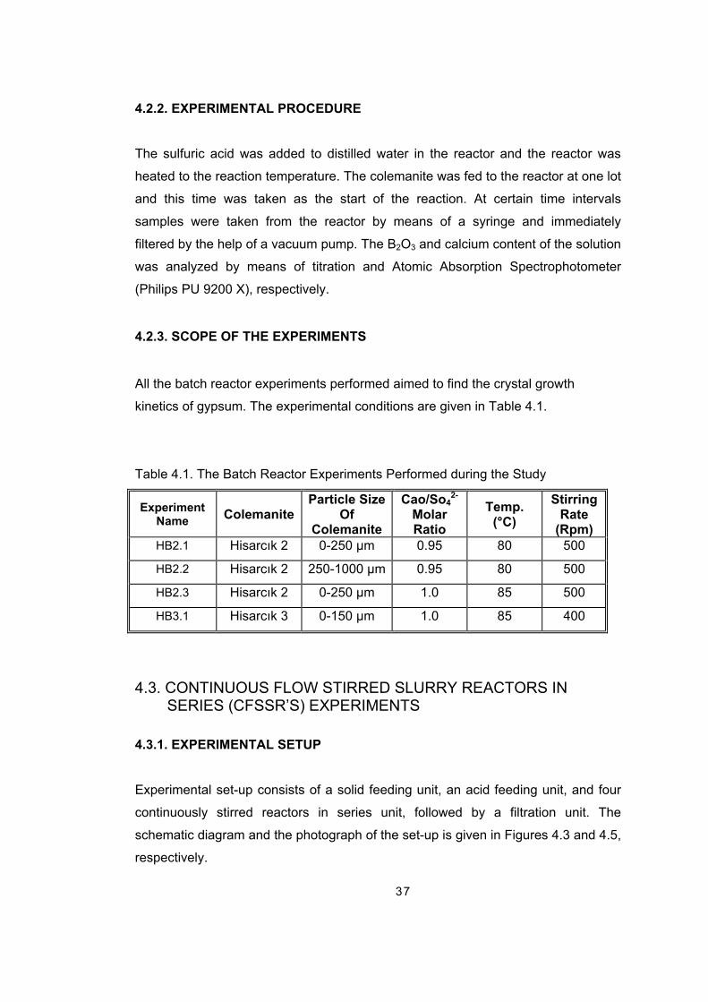
37
4.2.2. EXPERIMENTAL PROCEDURE
The sulfuric acid was added to distilled water in the reactor and the reactor was
heated to the reaction temperature. The colemanite was fed to the reactor at one lot
and this time was taken as the start of the reaction. At certain time intervals
samples were taken from the reactor by means of a syringe and immediately
filtered by the help of a vacuum pump. The B2O3 and calcium content of the solution
was analyzed by means of titration and Atomic Absorption Spectrophotometer
(Philips PU 9200 X), respectively.
4.2.3. SCOPE OF THE EXPERIMENTS
All the batch reactor experiments performed aimed to find the crystal growth
kinetics of gypsum. The experimental conditions are given in Table 4.1.
Table 4.1. The Batch Reactor Experiments Performed during the Study
Experiment Name Colemanite
Particle Size Of
Colemanite
Cao/So42-
Molar Ratio
Temp. (°C)
Stirring Rate
(Rpm) HB2.1 Hisarcık 2 0-250 µm 0.95 80 500
HB2.2 Hisarcık 2 250-1000 µm 0.95 80 500
HB2.3 Hisarcık 2 0-250 µm 1.0 85 500
HB3.1 Hisarcık 3 0-150 µm 1.0 85 400
4.3. CONTINUOUS FLOW STIRRED SLURRY REACTORS IN SERIES (CFSSR’S) EXPERIMENTS
4.3.1. EXPERIMENTAL SETUP Experimental set-up consists of a solid feeding unit, an acid feeding unit, and four
continuously stirred reactors in series unit, followed by a filtration unit. The
schematic diagram and the photograph of the set-up is given in Figures 4.3 and 4.5,
respectively.

38
The solid feeding unit consisted of three parts. The first part was the funnel, where
colemanite was put, the second part consisted of a mechanical stirrer (Heidolph
RZR 2041) connected to a screw type feeder, and the last part was the vibratory
feeder (Retsch DR 100). The colemanite falling from the funnel was first fed to the
screw type feeder, which carried it to the vibratory feeder. Colemanite, which fell to
the vibratory feeder, was then fed to the first reactor.
Acid feeding unit consisted of 100 l feed tank, a mechanical stirrer (Janke & Kunkel
K.C. RW38), a porcelain diver heater placed inside the tank, a temperature
controller (Elimko 200) and a thermocouple connected to the heater, and a
peristaltic pump (Watson Marlow 505S). Heated acid was fed to the first reactor by
means of the peristaltic pump.
The reactors are made up of glass (Çalışkan Cam, Ankara). The volume of each
reactor was 1.8 l. Each reactor was heated and continuously stirred. First reactor
had a silicone heating tape connected to a temperature controller (Isopad TD2000)
and a thermocouple. The other three reactors were jacketed and hot water was
circulated around each of them by means by a circulating water bath (Heto HWT
100, OBN 28). The techical drawing of one of the continuous flow stirred slurry
reactor is given in Figure 4.4, having hot water circulation around it. The dimensions
of the first reactor were the same, except the hot water circulation. In only
difference in the dimensions of the batch reactor was the height of the reactor, 30
cm, whereas the volume used in the reactor was 1.5 lt.
The temperatures of the reactors were measured by use of digital thermometers.
Stirring was done by means of mechanical stirrers and baffles were placed inside
the reactors for homogenous stirring. There were level differences between the
reactors and the outlet of one reactor was connected to the inlet of the next reactor
by means of overflows. The pH's of the reactors were recorded by the help of a pH-
meter (Mettler Toledo MP 200).
The outlet of the last reactor was connected to a filtration unit. The products, boric
acid (aqueous) and gypsum (solid) were separated by use of vacuum filtration. This
unit consisted of a vacuum pump (KNF NO22) connected to a 2 l nutsche flask and
a buhner funnel, having a 15 cm diameter, on top of it. Filter paper was placed on

39
the funnel and gypsum particles were collected on the filter paper whereas, boric
acid was collected in the flask.

40
Stream Input 1 Colemanite 2 Acid
Figure 4.3. Schematic diagram of the set-up used for the continuous flow stirred slurry reactor experiments
Circulating Water Bath
Peristaltic Pump
2
Mixer
TC
heater
Feed tank 8% H3BO3 5.58% H2SO4 86.42% H2O
Solid Feeder
Colemanite
1
Mixer
TC
Vacuum Pump
Mixer
Mixer
Mixer
Mixer
40

41
Figure 4.4. Technical drawing of the continuous flow stirred slurry reactor
12 cm
6 cm
6 cm
6 cm
1.5 cm
15 cm
12 mm
Hot water
inlet
Hot water
outlet

42
Figure 4.5. Photograph of the set-up used for the continuous flow stirred slurry reactor experiments
42

43
4.3.2. DYNAMIC BEHAVIOR EXPERIMENTS
4.3.2.1. EXPERIMENTAL PROCEDURE The experiments were all performed by using a single CSTR, the volume of which
was 1840 ml. In all dynamic behavior experiments, in other words residence time
distribution experiments, distilled water was used with a flow rate of 42.5 ml/min,
i.e., there was no reaction in the reactor system (sulfuric acid has not been added).
First of all, in order to check if the CSTR that was used during the experiments
approached an ideal one, the liquid residence time experiments were performed by
injecting nickel to the inlet stream as a pulse tracer. In the experiments the data
was taken by mixing cup readings, that is, the effluent of the reactor was collected
in flasks for 10 min intervals and samples were taken from each flask. The nickel
concentration of each sample was determined by means of Atomic Absorption
Spectrophotometer (Philips PU 9200 X).
Two different stirring rates, namely 500 and 750 rpm, were applied to the same
system to see the effect of the stirring rate on the residence time of the liquid. Also
two different tracers, lithium and nickel were given to the system at a stirring rate of
500 rpm to check different tracers.
The behavior of a single CSTR to the step tracer of colemanite was studied at 500
rpm either giving 4.3 g/min colemanite to the system or preventing the colemanite
flow and taking mixing cup readings, that is, the effluent of the reactor was filtered
for 5 min intervals and waited to dry to see the amount of colemanite collected.
The behavior of a CSTR to a pulse tracer of lithium when both liquid and colemanite
was flowing at steady state was searched at two different stirring rates (500, 750
rpm). The colemanite and water flow rates were 7.2 g/min and 42.5 ml/min,
respectively. Mixing cup readings were taken, that is, the effluent of the reactor was
collected in flasks for 10 min intervals and after the precipitation of the colemanite,
and samples were taken from the liquid part of each flask. The colemanite used in
the experiments was Hisarcık1 colemanite. The lithium amount of the Hisarcık1
colemanite was 0.028%.

44
Same procedure was repeated at 500 rpm with different solid to liquid ratios (0.085,
0.17, 0.34). For these cases, the flow rate of colemanite kept constant at 7.2 g/min,
while the flow rate of water changed (84.7, 42.5, 21.2 g/min).
4.3.2.2. SCOPE OF THE EXPERIMENTS The dynamic behavior experiments were performed as shown in Table 4.2.
Table 4.2. Dynamic Behavior Experiments Performed
Set 1: Liquid Residence Time Experiments
Experiment Name
Tracer (Pulse)
Liquid Feed Rate
(g/min)
Solid* Feed Rate
(g/min)
Stirring Rate (rpm)
HC1.1 Nickel 42.5 - 500
HC1.2 Nickel 42.5 - 750
HC1.3 Lithium 42.5 - 500
SET 2: SOLID RESIDENCE TIME EXPERIMENTS
Experiment Name
Tracer (Step)
Liquid Feed Rate
(g/min)
Solid* Feed Rate
(g/min)
Stirring Rate (rpm)
HC1.4 Colemanite (negative input)
- 4.3 500
HC1.5 Colemanite (positive input)
- 4.3 500
SET 3: LIQUID RESIDENCE TIME EXPERIMENTS IN A SOLID/LIQUID SYSTEM
Experiment Name
Tracer (Pulse)
Liquid Feed Rate
(g/min)
Solid* Feed Rate
(g/min)
Stirring Rate (rpm)
HC1.6 Lithium 42.5 7.2 500
HC1.7 Lithium 42.5 7.2 750
HC1.8 Lithium 84.7 7.2 500
HC1.9 Lithium 21.2 7.2 500 * Solid used in the experiments is Hisarcık 1, 0-250 µm, colemanite.

45
4.3.3. BORIC ACID PRODUCTION EXPERIMENTS
4.3.3.1. EXPERIMENTAL PROCEDURE
The water bath and the feed tank were heated to the desired temperatures of 90°C
and 85°C, respectively. While they were heating, 16% boric acid solutions were
prepared and also heated to 85°C by the use of magnetic stirrers with heater
(Heidolph MR 3001). Distilled water was used for this preparation. Tap water was
distilled by the use of a water distillation apparatus (Nüve NS 108).
On the other hand, solid and acid feeding units were calibrated before the
experiments. It was critical to use dry colemanite during the experiments, so
colemanite was stored at 85°C in the oven (Nüve FN 500) till the rest of the
experiments.
The hot water was circulated through the jackets of the last three reactors, where
hot water inlet was from the last reactor. At the same time, the controller of the
silicone heating tape was adjusted to 85°C in the first reactor. Then, hot 16% boric
acid solutions were put into the first three reactors. The last reactor was left empty.
At the beginning of the experiment, the colemanite and acid feeders were operated
at the same time and this time was accepted as the zero time, which describes the
starting moment of the reaction. Samples were begun to be taken when the first
product was taken from the last reactor. The samples are taken in time intervals.
Colemanite and acid feeding was checked continuously and feeding of colemanite
to the solid feeder funnel and acid to the acid tank was done in appropriate
intervals.
During the experiments, samples were withdrawn from all of the reactors by means
of a 50 ml syringe attached to a 15 cm long glass pipe. The samples were
immediately filtered by a filtration unit resembling the one described in the
experimental set-up for product filtration. In this unit, analytical funnels were placed
above 250 ml nutsche flasks and this apparatus was put into hot water, in order to
prevent the boric acid solution to crystallize. Blue band filter papers were put on the

46
funnels and solid particles were collected on it. Samples for examining the boric
acid and calcium ions in solution were taken from the flask by the help of 5 ml and 1
ml micropipettes (Finpipette, Thermo Labsystems), respectively.
The filtration process should be quick to prevent boric acid to crystallize on the filter
paper. So, the procedure explained for filtration was not applicable to the systems
having high solid hold-ups. For such systems, another filtration system, which was
by using syringe filters, was adapted to the system to find the boric acid and
calcium ion concentrations in the solution. The syringe filters were first put into the
oven until they reach a temperature of 85°C, the same temperature with the slurry.
Then, the slurry, taken by the syringe was filtered by inserting the tip of the syringe
to the filter.
The temperatures of the reactors and the pH values were recorded during the
experiments. The pH values of the reactors were used in determining if the reactor
comes to steady state or not.
The samples of the boric acid solution were taken from the flask when the system
comes to steady state. These samples were analyzed for the sulfate ion and
magnesium ion concentrations.
4.3.3.2. SCOPE OF THE EXPERIMENTS The parameters that were not changed during the experiments were listed below:
- The concentration of sulfuric acid (5.58%) and boric acid (8%) in the feed
tank
- Stirring rate of the reactors (400 rpm)
- Temperature of the reactors and the feed tank (82°C– 85°C in reactors,
85°C in the feed tank)
- Initial boric acid concentration (16%) put in the first three reactors
Three sets of experiments were performed during the study. In two sets of the
experiments, the changes in the flow rates of the colemanite and acid were used to
observe the changes in the sizes of gypsum crystals. While changing the flow rates

47
of colemanite and acid, CaO/SO42- molar ratio and solid hold-up values, hs, was
constant.
In the last set of the experiments, CaO / SO42- molar ratio and solid hold-up values,
hs were changed. These two ratios were very critical in this study. So, the effect of
these ratios was observed by changing the acid feed rates at constant colemanite
feed rate. The performed experiments are tabulated in Table 4.3a and 4.3b.
Table 4.3a. Performed Experiments in Grouped Style in Continuous Flow Stirred Slurry Reactors in Series
COLEMANİTE USED CONDİTİONS
COLEMANİTE FEED RATE
(G/MİN)
ACİD FEED RATE
(G/MİN) 5 48.5
7.5 72.7 CaO/SO4
2- : 1.00 hs : 0.04
10 97
5 35
10 70 CaO/SO4
2- : 1.37 hs : 0.06
15 105
Hisarcık2 (0-250 µm)
CaO/SO42- : 2.17
hs : 0.09 10 45
3.5 30 Hisarcık 3 (0-150 µm)
CaO/SO42- : 1.00
hs : 0.05 10 90

48
Table 4.3b. Performed Experiments in Continuous Flow Stirred Slurry Reactors in Series
EXPERİMENT NAME COLEMANİTE PARTİCLE SİZE OF
COLEMANİTE CAO/SO4
2- MOLAR FLOW
RATE SOLİD HOLD-
UP, HS COLEMANİTE FEED RATE
(G/MİN)
ACİD FEED RATE
(G/MİN) HC2.1 Hisarcık 2 0-250 µm 1.00 0.04 5 48.5
HC2.2 Hisarcık 2 0-250 µm 1.00 0.04 7.5 72.7
HC2.3 Hisarcık 2 0-250 µm 1.00 0.04 10 97
HC2.4 Hisarcık 2 0-250 µm 1.37 0.06 5 35
HC2.5 Hisarcık 2 0-250 µm 1.37 0.06 10 70
HC2.6* Hisarcık 2 0-250 µm 1.37 0.06 10 70
HC2.7 Hisarcık 2 0-250 µm 1.37 0.06 15 105
HC2.8 Hisarcık 2 0-250 µm 2.17 0.09 10 45
HC3.1 Hisarcık 3 0-150 µm 1.00 0.05 3.5 30
HC3.2 Hisarcık 3 0-150 µm 1.00 0.05 10 90
* Experiment H2.6 was performed for the reproducibility analysis
48

49
4.4. ANALYTICAL PROCEDURES
4.4.1. DETERMINATION OF BORIC ACID CONCENTRATION
The boric acid concentration of the liquid phase was determined as follows: 5 ml of
sample was taken from the solution, which was filtered by using blue band filter,
and put into a bottle. Methyl red indicator was put on it and 1-2 drops of 1:3 (by vol.)
H2SO4 was added to the solution. Then, 6 N NaOH was put until the color changes
from pink to yellow. After this step, H2SO4 was again added to the solution until the
color turns back to pink. This solution is titrated with 0.5 N NaOH until a pH of 4.5 is
obtained. At this step a titrator involving a magnetic stirrer and pH-meter (TitroLine
easy, Schott) was used to get accurate results. Then, phenolphtalein indicator was
put into the bottle and 10-15 g mannitol was added to the solution. The solution was
again titrated with 0.5 N NaOH until the pH of the solution becomes 8.5. The
volume of the NaOH used in this step was recorded and used to calculate the boric
acid concentration from the following formula:
H3BO3 (mol/l) = VNaOH FNaOH NNaOH / Vsample
where VNaOH, FNaOH, NNaOH and Vsample are the volume of the NaOH used, factor of
the NaOH, normality of NaOH, and the volume of the sample, respectively.
4.4.2. DETERMINATION OF CALCIUM ION CONCENTRATION Calcium ion concentration of the samples was determined by Atomic Absorption
Spectrophotometer (Philips PU 9200X) in METU Chemical Engineering
Department. 1 ml samples were taken to the 100 ml plastic balloon georgette and
deionized water was added on the sample. The liquid samples were directly
measured at atomic absorption spectrophotometer after diluting the sample to a
maximum of 15 ppm. Before each analysis the atomic absorption
spectrophotometer was calibrated between 0 - 15 ppm calcium content.
4.4.3. DETERMINATION OF SULFATE ION CONCENTRATION Sulfate ion in solution was determined gravimetrically. The procedure was as
follows:

50
The solution was filtered and from the filtrate 25 ml was taken. 10 ml HCl, 1 ml 3%
H2O2 and methyl red indicator was added to the solution. The solution was boiled to
oxide the R2O3 groups, which are iron, aluminum and titanium. It was continued to
boil until a remaining red color was seen in the solution. The solution was
precipitated by adding drop by drop 1:1 (by vol.) NH4OH. The solution having a
yellow color was boiled on hot plate for 5 minutes. The solution was filtered and the
filtrate was taken. 10 ml HCl, 25 ml 10% hot BaCl2 and methyl red indicator was
added to the solution. The solution was precipitated as BaSO4 by stirring. The
solution was then left on hot plate for one hour. Then, the solution was taken and
waited overnight. After that, the solution was filtered and washed with hot water.
The solution was put into constant weight crucible and weighed. The crucible was
then put into the oven and heated to 850°C. The crucible was left at 850°C for one
hour and then weighed. The weight difference will give the amount of BaSO4. The
BaSO4 amount was then converted to sulfate ion concentration.
4.4.4. DETERMINATION OF MAGNESIUM ION CONCENTRATION Magnesium ion concentration of the samples was determined by Atomic Absorption
Spectrophotometer (Philips PU 9200X) in METU Chemical Engineering
Department. The liquid samples were directly measured at atomic absorption
spectrophotometer after diluting the sample to a maximum of 0.9 ppm. Before each
analysis the atomic absorption spectrophotometer was calibrated between 0.3 – 0.9
ppm magnesium content.
4.4.5. CRYSTAL SIZE DETERMINATION
4.4.5.1. PARTICLE SIZE DISTRIBUTION OF GYPSUM CRYSTALS When the system comes to steady state, the pH of the slurry was constant;
samples were taken from all of the reactors and filtered. These samples were
washed during filtration to get rid of the boric acid in the filtrate. The solid collected
from the reactors were further washed by putting a small amount of solid into a
large volume of water and stirred. The solid was then again filtered and put into
sample bottles. Water was also added to the bottles. Tap water used was used
during the analysis.

51
The particle size distributions of the solid samples were determined by a particle
size analyzer (Malvern Instruments, Mastersizer 2000), in Ankara University,
Chemical Engineering Department, utilizing the principle of laser ensemble light
scattering. This instrument can detect the particle range of 0.02-2000 µm. The
analysis was done by using wet dispersion method with a repeatability of +/- 0.5%.
The dispersant used in the analysis was tap water.
In the analysis, some amount of solid was taken from the sample bottles and put
into 800 ml beaker filled with water. This beaker was put on its place in the
analyzer. Solid was continued to be added until the laser obscuration value on the
computer reaches 14-15%. Then the analyzer was ready to give the crystal size
distribution of the sample. The analysis was repeated for three times to see if the
same result was obtained or not. It was seen that reproducible results were
obtained. Then, the volume weighted mean of the curves were calculated by the
software of the analyzer.
4.4.5.2. LIGHT MICROSCOPE IMAGES OF GYPSUM CRYSTALS
The colemanite particles were examined under the light microscope. In the
analysis, Prior Laboratory Microscope Model B 3000 was used. Microscope was
connected online to a computer by Pro Series, high performance CCD camera.
Images were seen live in monitor by an analytical imaging software called Image
Pro Plus 3.0 for Windows. The views of the samples were snapped and saved into
the computer.

52
CHAPTER 5
RESULTS AND DISCUSSION
5.1. RESULTS OF COLEMANITE ANALYSIS
5.1.1. SCREEN ANALYSIS OF COLEMANITE
Colemanite, named as Hisarcık 1, had average particle sizes of 2.5 cm. Colemanite
is first crushed in the jaw crusher and then ground in a hammer mill. To get the size
distribution, sieve analysis is performed. In previous experiments, performed by
Çetin et. al (2001) particles smaller than 250 µm was used. So, the first sieve
analysis is performed to see the amount of the colemanite left on the 60 mesh sieve
(corresponding to 250 µm). It was seen that nearly 35 percent of the colemanite
was left on this sieve. It is seen that the maximum particle diameter of the
colemanite is between 1-2 mm (18-10 mesh, respectively). The screen analysis of
the Hisarcık 1 colemanite is given in Table 5.1.1, in which the mass fractions of the
colemanite on each sieve and the cumulative mass fractions of the colemanite
under that sieve were given. The particle diameter is the maximum diameter of the
particles that could pass the former sieve. The average particle diameter stands for
the arithmetic mean of the minimum and maximum diameter of the particles on that
sieve. Figure 5.1.1 presents the differential particle size distribution of the Hisarcık 1
colemanite particles sieved. The mass fraction of the colemanite particles on each
sieve according to their average particle diameters were illustrated, whereas Figure
5.1.2 illustrates the particle size distribution of the Hisarcık 1 colemanite particles by
the cumulative amount of the colemanite particles under the stated particle
diameters. For each particle diameter, cumulative mass fraction of the colemanite
smaller than that diameter is given.

53
Table 5.1.1. The screen analysis of Hisarcık 1 colemanite
Mesh No Dpi, µm Mass Fraction Avg. Dpi, µm Cum. Mass Fraction 25 710 0.056 - 0.944 35 500 0.070 605 0.874 45 355 0.140 428 0.734 60 250 0.074 303 0.660 70 212 0.053 231 0.607
100 150 0.152 181 0.455 120 125 0.013 138 0.441 pan - 0.441 63 0.000
0.0
0.1
0.2
0.3
0.4
0.5
63 138 181 231 303 428 605
Mas
s fr
actio
n by
wei
ght
Average particle diameter, µm
Figure 5.1.1. Particle size distribution curve (differential analysis) for Hisarcık 1 colemanite

54
0,00,1
0,20,3
0,40,50,6
0,70,8
0,91,0
0 100 200 300 400 500 600 700 800
Particle Diameter, µm
Cum
ulat
ive
frac
tion
smal
ler t
han
Dpi
Figure 5.1.2. Particle size distribution curve (cumulative analysis) for Hisarcık 1 colemanite
The colemanite named as Hisarcık 2, arrived under the name of 25-100 mm, which
denotes its size. The sieve analysis of it was also performed and given in Table
5.1.2. the differential and cumulative analysis are shown in Figures 5.1.3 and 5.1.4,
respectively.
Table 5.1.2. The screen analysis of Hisarcık 2 colemanite
Mesh No Dpi, µm Mass Fraction Avg. Dpi, µm Cum. Mass Fraction
25 710 0.054 - 0.946 35 500 0.085 605 0.860 45 355 0.087 428 0.773 60 250 0.049 303 0.724
100 150 0.373 200 0.350 140 106 0.170 128 0.180 170 90 0.075 98 0.105 270 53 0.063 45 0.042 pan - 0.042 27 0.000

55
0.0
0.1
0.2
0.3
0.4
27 45 98 128 200 303 428 605
Mas
s fr
actio
n by
wei
ght
Average particle diameter, µm
Figure 5.1.3. Particle size distribution curve (differential analysis) for Hisarcık 2 colemanite
0.0
0.1
0.2
0.3
0.4
0.5
0.6
0.7
0.8
0.9
1.0
0 100 200 300 400 500 600 700 800Particle Diameter, µ m
Cum
ulat
ive
frac
tion
smal
ler
than
D
pi
Figure 5.1.4. Particle size distribution curve (cumulative analysis) for Hisarcık 2 colemanite
Hisarcık 3 colemanite was brought from Emet Boric Acid Plant. The maximum
diameter of the colemanite minerals was 150 µm. Therefore, no size reduction was
necessary. The screen analysis of the Hisarcık 3 colemanite is given in Table 51.3.

56
Figure 5.1.5 and Figure 5.1.6 present the differential particle size distribution and
the cumulative particle size distribution of the Hisarcık 3 colemanite respectively.
Table 5.1.3. The screen analysis of Hisarcık 3 colemanite
Mesh No Dpi, µm Mass Fraction Avg. Dpi, µm Cum. Mass Fraction
100 150 0.134 - 0.866 140 106 0.243 128 0.623 170 90 0.325 98 0.298 270 53 0.117 72 0.181 pan - 0.181 26.5 0
0
0,1
0,2
0,3
0,4
26,5 72 98 128
Average particle diameter, mm
Mas
s fr
actio
n by
wei
ght
Figure 5.1.5. Particle size distribution curve (differential analysis) for Hisarcık 3 colemanite

57
0,0
0,1
0,2
0,3
0,4
0,5
0,6
0,7
0,8
0,9
1,0
0 20 40 60 80 100 120 140 160Particle diameter, µm
Cum
ulat
ive
frac
tion
smal
ler t
han
Dp i
Figure 5.1.6 Particle size distribution curve (cumulative analysis) for Hisarcık 3 colemanite
5.1.2. CHEMICAL ANALYSIS OF COLEMANITE
To see if the size of the colemanite changes the chemical composition, the
chemical analysis of Hisarcık 1 colemanite was done on different sizes, 250-1000
µm, 0 -250 µm and 0-1000 µm. The size named as 0-1000 µm is the hammer mill
product consisting of 35% colemanite greater than 250 µm. The chemical analysis
of the colemanites is given in Appendix A. The chemical composition of Hisarcık 1
colemanite is given in Table 5.1.3.

58
Table 5.1.4. Chemical analysis of Hisarcık 1 colemanite (dry basis, wt%) (METU, Chemical Eng. Dept.)
Component 250-1000 µm 0 - 250 µm 0-1000 µm
B2O3 39.17 37.72 38.53
CaO 23.63 24.23 22.25
Na2O 0.58 0.78 0.17
MgO 1.92 1.93 2.19
Al2O3 1.77 1.48 1.69
SiO2 18.51 19.71 7.72
Fe2O3 1.06 0.84 1.06
As2O3 0.59 0.51 0.55
SrO 0.88 1.03 0.94
TiO2 0.13 0.11 0.11
K2O 2.27 1.55 1.55
BaO 0.02 0.02 0.02
Others 9.47 10.09 23.22
As seen from this table, the change in the particle size did not change the analysis
results significantly, especially the calcium oxide and boron trioxide results did not
differ much, which are important values for the experiments. CaO/B2O3 ratio is a
critical value for the case of the amount of sulfuric acid addition. As sulfuric acid
amount changes the calcium ion concentration changes with respect to time (Çetin
et.al., 2001).
The chemical analysis of Hisarcık 2 and Hisarcık 3 colemanites were also done.
The comparison of different colemanites, together with the published ones by
Kalafatoğlu et.al, 2000 and Özkan, 1999, is also given in Table 5.1.4.

59
Table 5.1.5. Chemical analysis of Hisarcık colemanites (dry basis, wt%) (METU, Chemical Eng. Dept.)
Component Hisarcık 1 Colemanite
Hisarcık 2 Colemanite
Hisarcık 3 Colemanite
Kalafatoğlu et. al., 2000
Özkan, 1999
B2O3 38.53 43.57 34.61 43.10 43.69
CaO 22.25 30.90 28.41 25.77 20.50
Na2O 0.17 0.22 1.30 0.17 0.06
MgO 2.19 0.79 2.36 2.09 1.18
Al2O3 1.69 0.22 1.49 1.27 0.86
SiO2 7.72 0.60 2.23 5.84 3.77
SO3 0.14 0.65 1.14 0.21
Fe2O3 1.06 0.17 0.61 0.59 0.31
As2O3 0.55 0.00 0.42 0.25 2.00
SrO 0.94 0.56 0.88 1.17 1.55
TiO2 0.11 0.20 0.14 0.02
K2O 1.55 0.08 0.74 0.42 0.19
BaO 0.02 0.005 0.017 0.01
Li 0.028 0.045
Others 23.22 22.50 26.13 18.16 25.68
As seen from Table 5.1.4, Hisarcık 2 colemanite is the most valuable one among
the three colemanites used in the study due to its boron trioxide content. The boron
trioxide content of Hisarcık 3 colemanite, on the other hand, was the lowest among
all other colemanites.
5.1.3. PARTICLE SIZE DISTRIBUTION OF COLEMANITE
The particle size distribution of the colemanite was also examined with the laser
diffraction particle size analyzer. The particle size distribution of the colemanites
used in the study are given in the Figures 5.1.5 - 5.1.7 for Hisarcık 1, Hisarcık 2 and
Hisarcık 3 colemanites, having particle sizes determined from the screen analysis
as 0-250 µm, 0-250 µm and 0-150 µm, respectively.

60
Particle Size Distribution
0.01 0.1 1 10 100 1000 3000 Particle Size (µm)
0 1 2 3 4 5 6 7 8
Vol
ume
(%)
Figures 5.1.7. Particle size distribution of Hisarcık 1 colemanite
Particle Size Distribution
0.01 0.1 1 10 100 1000 3000 Particle Size (µm)
0
1
2
3
4
5
Vol
ume
(%)
Figures 5.1.8. Particle size distribution of Hisarcık 2 colemanite
Particle Size Distribution
0.01 0.1 1 10 100 1000 3000 Particle Size (µm)
0 0.5
1 1.5
2 2.5
3 3.5
4 4.5
Vol
ume
(%)
Figures 5.1.9. Particle size distribution of Hisarcık 3 colemanite

61
The particle size distribution of the colemanites, Figures 5.1.5-5.1.7, did not give
particle sizes similar to that of the screen analysis. In laser diffraction particle size
analyzer, the shapes of the particles are taken as a sphere, and the volumes are
calculated accordingly. The volume weighted mean diameter, also called as the De
Broucker mean, was generated by the laser diffraction instrument, which was the
arithmetic average of the diameters of the colemanites. The volume weighted mean
diameters obtained from the software of the particle size analyzer are given in
Table 5.1.5.
Table 5.1.6. Volume weighted mean diameters of the colemanites
Colemanite Particle Size Obtained From Sieve Analysis
Mean Diameter Of Colemanite Obtained From
Particle Size Analyzer Hisarcık 1 0-250 µm 44.53 µm
Hisarcık 2 0-250 µm 113.13 µm
Hisarcık 3 0-150 µm 73.56 µm
Hisarcık 1 colemanite was used for the dynamic behavior experiments, Hisarcık 2
and Hisarcık 3 were used for the boric acid production in batch and continuous
reactor experiments. The second column in Table 5.1.5 is the size obtained from
the sieve analysis, and gives the diameter range of the colemanite particles. The
last column is the volume weighted mean diameter of the colemanite particles. As
seen, the mean diameters found from the analyzer are in the range of the diameters
obtained from the sieve analysis.
5.2. DYNAMIC BEHAVIOR EXPERIMENTS ON CONTINUOUS FLOW STIRRED SLURRY REACTORS
There are two ideal patterns, plug flow and mixed flow. These can give very
different behavior like the size of the reactor and distribution of the products. These
two patterns are simple to treat and one or the other is often optimum no matter
what we are designing for. But real equipment always deviates from these ideals.
Deviation from these ideal patterns can be caused by channeling of fluid, by

62
recycling of fluid, or by creation of stagnant regions in the vessel. These behaviors
can be found by performing residence time distribution, RTD, experiments. These
non-idealities should be avoided since it always lowers the performance of the
reactors. In order to check the performance of the slurry reactors residence time
distribution experiments were performed in either a liquid or a solid-liquid system.
During the RTD experiments a non reactive tracer was chosen and it is given as a
pulse or a step input. After giving a tracer to the system, concentration of the tracer
at the effluent stream was recorded with respect to time, and C(t) curves were
analyzed to detect the nonidealities in the reactor.
5.2.1. LİQUİD RESİDENCE TİME EXPERİMENTS
Dynamic behavior studies were performed by using only one continuously stirred
baffled tank reactor having a volume of 1840 ml. Various parameters were selected
and applied to the experiments to see their effects on the residence time
distribution.
5.2.1.1. EFFECT OF STİRRİNG RATE ON LİQUİD RESİDENCE TİME
The tank reactor was stirred by means of a mechanical stirrer. The peristaltic pump
was connected to the inlet fluid stream to have a constant liquid feed rate of 42.5
ml/min. For the fluid stream distilled water was used throughout the residence time
experiments.
In the first experiment, nickel, 1000 ppm, was injected to the inlet stream, as an
inert tracer with a volume of 10 ml. Two different stirring rates were applied to the
system to see the effect of stirring rate on the residence time distribution. In both
experiments the data was taken by mixing cup readings. The data is given in
Appendix B, Table B.1. The results of the two experiments are given in Figure 5.2.1
for comparison. The plot was also named as Cpulse curve.

63
0
1
2
3
4
5
6
0 50 100 150 200 250 300Time, min
Nic
kel C
once
ntra
tion,
ppm 500 rpm
750 rpm
Figure 5.2.1. Variation in nickel concentration depending on the stirring rate during the liquid residence time experiments (Volumetric flow rate = 42.5 ml/min) The area under the Cpulse curve is calculated as follows:
υMtCtdCA
iii =∆≅= ∑∫
∞
0
(5.2.1)
where A is the area under the Cpulse curve, M is the amount of tracer in kg and υ:
volumetric flow rate of liquid in m3/s. To find the residence time distribution, E(t)
from the Cpulse curve, the concentration scale was simply changed such that the
area under the curve is unity.
υMC
tE pulse=)( (5.2.2)
The normalization of the experimental data was done by the use of equations 5.2.1
and 5.2.2.
The E(t) curves at two stirring rates, 500 rpm and 750 rpm are given in Figure 5.2.2.
By using the E(t) values, F(t) values were also calculated from Equation 5.2.3.
( ) ( )∫=t
tdtEtF0
(5.2.3)
The F(t) curves are given in Figure 5.2.3. The E(t) and F(t) values for the
experiments are given in Table B.2.

64
To see if the reactor approaches an ideal one or not, the E(t) and F(t) curves for an
ideal CSTR reactor was drawn and compared with the experimentally found ones.
During the calculation of E(t) and F(t) values for an ideal reactor, the equations
used were
i
t ietEτ
τ/)(
−= (5.2.4)
F(t) equation was found by using Equations 5.2.3, i.e., taking the integral of the E(t)
equation, which is:
itetF τ/1)( −−= (5.2.5)
The ideal reactor’s E(t) and F(t) curves are also drawn in Figure 5.2.2-5.2.3,
respectively. The values for E(t) and F(t) are given in Table B.2.
0,000
0,005
0,010
0,015
0,020
0,025
0 50 100 150 200 250 300Time, min
E (t)
500 rpm
750 rpm
Ideal CSTR
Figure 5.2.2. Comparison of the E(t) curves for two different stirring rates and the ideal reactor

65
0,0
0,2
0,4
0,6
0,8
1,0
0 50 100 150 200 250 300Time, min
F (t)
500 rpm
750 rpm
Ideal CSTR
Figure 5.2.3. Comparison of the F(t) curves for two different stirring rates and the ideal reactor
It can be seen from Figure 5.2.2 and 5.2.3 that the reactor used in the experiments
was an ideal reactor and stirring rate studied had no effect on the liquid residence
time.
The residence time, τ, was calculated by Equation 5.2.6 as τ = V/υ. The mean of
the Cpulse curve was also calculated by Equation 5.2.6, but this time the
experimental data was used. The two values should be equal to each other.
υV
tC
tCt
tdC
tdCtt
iii
iiii
=∆
∆
≅=∑∑
∫∫
∞
∞
0
0 (5.2.6)
The values calculated without the experimental data were called theoretical values.
Variance, which shows the spread of the curves, was also calculated from Equation
5.2.7.
( ) 22
2
0
02
2 ttC
tCt
ttdC
tdCt
iii
iiii
−∆
∆
≅−=∑
∑
∫∫
∞
∞
σ (5.2.7)
The mean of the curve, area under the curve and the variance per square of the
mean of the curves are compared in Table 5.2.1.

66
Table 5.2.1. Comparison of the two experimental values with the theoretical ones (volumetric flow rate = 42.5 ml/min, tracer= nickel)
Experimental Theoretical
Stirring Rate 500 rpm 750 rpm
A, g.min /l 0.265 0.205 0.235
t , min 43.5 43.7 43.3
22 / tσ 0.91 0.88
The data for the mean residence time for all the cases seemed to be close to each
other. It can be stated that the experimentally evaluated data parallels with the
theoretical ones.
5.2.1.2. CHECK OF DIFFERENT TRACERS ON LİQUİD RESİDENCE TİME
In liquid residence time experiments where colemanite was used as a solid, lithium
was used as an inert tracer. For this reason, the liquid residence time experiment
was repeated by using lithium and the usage of different tracers were checked.
Liquid residence time experiment HC1.1, stirring rate of 500 rpm, was repeated with
the same amount of lithium instead of nickel to see the difference, if any, between
the results. The concentration values of the tracers are compared in Figure 5.2.4,
and the data is given in Table B.3.
0
1
2
3
4
5
6
0 50 100 150 200 250 300 Time, min
Con
cent
ratio
n, p
pm
Lithium
Nickel
Figure 5.2.4. Comparison of concentrations of different tracers

67
To normalize the concentration values, E(t) and F(t) curves are drawn and
compared with the ideal CSTR in Figures 5.2.5-5.2.6, respectively. E(t) and F(t)
values are tabulated in Table B.4.
0,000
0,005
0,010
0,015
0,020
0,025
0 50 100 150 200 250 300
Time, min
E(t)
LithiumNickelIdeal CSTR
Figure 5.2.5. Comparison of the E(t) curves for different tracers and the ideal reactor
0,0
0,2
0,4
0,6
0,8
1,0
0 50 100 150 200 250 300 Time, min
F(t)
LithiumNickelIdeal CSTR
Figure 5.2.6. Comparison of the F(t) curves for different tracers and the ideal reactor
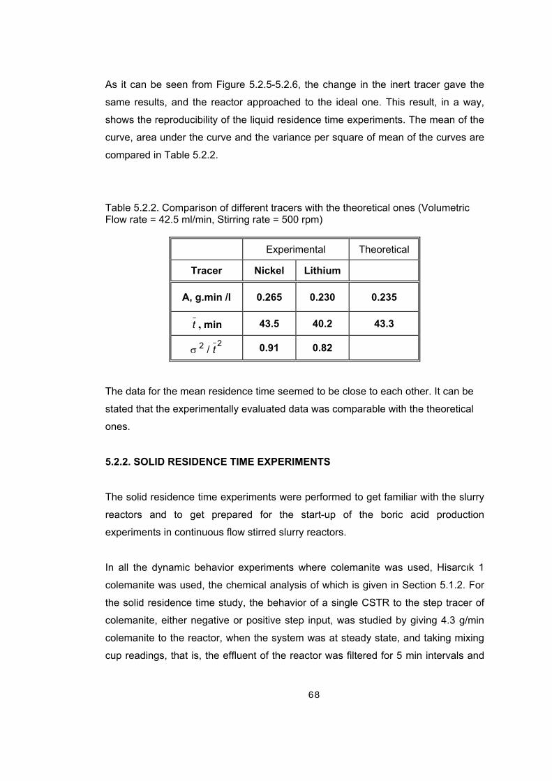
68
As it can be seen from Figure 5.2.5-5.2.6, the change in the inert tracer gave the
same results, and the reactor approached to the ideal one. This result, in a way,
shows the reproducibility of the liquid residence time experiments. The mean of the
curve, area under the curve and the variance per square of mean of the curves are
compared in Table 5.2.2.
Table 5.2.2. Comparison of different tracers with the theoretical ones (Volumetric Flow rate = 42.5 ml/min, Stirring rate = 500 rpm)
Experimental Theoretical
Tracer Nickel Lithium
A, g.min /l 0.265 0.230 0.235
t , min 43.5 40.2 43.3
22 / tσ 0.91 0.82
The data for the mean residence time seemed to be close to each other. It can be
stated that the experimentally evaluated data was comparable with the theoretical
ones.
5.2.2. SOLID RESIDENCE TIME EXPERIMENTS
The solid residence time experiments were performed to get familiar with the slurry
reactors and to get prepared for the start-up of the boric acid production
experiments in continuous flow stirred slurry reactors.
In all the dynamic behavior experiments where colemanite was used, Hisarcık 1
colemanite was used, the chemical analysis of which is given in Section 5.1.2. For
the solid residence time study, the behavior of a single CSTR to the step tracer of
colemanite, either negative or positive step input, was studied by giving 4.3 g/min
colemanite to the reactor, when the system was at steady state, and taking mixing
cup readings, that is, the effluent of the reactor was filtered for 5 min intervals and

69
dried to see the amount of colemanite collected. The stirring rate during the
experiments was 500 rpm.
The data for two experiments are given in Appendix B, Table B.5. The comparison
of negative and positive step inputs to the same system are given in Figure 5.2.7.
0
5
10
15
20
25
0 50 100 150 200
Time, min
Col
eman
ite w
eigh
t, g
negative steppositive step
Figure 5.2.7. Responses to a negative and a positive step input given to the feed rate of colemanite As seen from Figure 5.2.7, the data for negative and positive step input
experiments resembled each other. The residence time, and the variance was
calculated by using the equations 5.2.8-5.2.9, respectively.
( ) ( )
max
1max
max
0 max
C
tCC
C
tdCCt i
ii
∆
∆−
=∆
−=
∑∫ =
∞
(5.2.8)
( ) 2
max
02
2
max
0 max2max2
tC
Cdtt
C
tdCCtC
−∆
=−∆
−⋅=
∫∫∞
σ (5.2.9)
In equations 5.2.8-5.2.9, Cmax values for negative and positive step tracers were
21.3 g for each of the experiments, which was equal to the amount of colemanite
Dis
turb
ance

70
collected in five minutes. The theoretical calculation of Cmax and mean residence
time is given in Equations 5.2.10 and 5.2.11, respectively.
υmC =max (5.2.10)
Area = 2max
υ
VmtC = (5.2.11)
The mean residence time was calculated from equations 5.2.10 and 5.2.11 as 43.8
min. The comparisons of the experimental and theoretical values are given in Table
5.2.3.
Table 5.2.3. Comparison of the residence time and the variance per square of residence time for step input experiments
Experimental Theoretical
Step Input Negative Positive
t , min 96.3 46.2 43.8
22 / tσ 0.12 0.12
The mean residence times evaluated from the negative and positive step response
experiments should give similar values but they were found different as seen from
Table 5.2.3. The reason for this difference was that for the negative step
experiment, as the amount of solid decreased in the reactor, the readings were still
taken. During the calculations, the area was found greater than that of the positive
step experiments, which makes the mean residence time higher. The mean
residence time found for the positive step input experiment was close to the
theoretical calculation. So, while studying solid residence time experimentally,
giving a positive step input is recommended.

71
5.2.3. LİQUİD RESİDENCE TİME EXPERİMENTS İN A SOLİD/LİQUİD SYSTEM
When distilled water was fed together with colemanite, a pulse tracer of nickel,
1000 ppm, was injected to the liquid stream. The atomic absorption
spectrophotometer results of nickel analysis showed that, nickel was adsorbed on
the colemanite. And all the nickel in the solution was completely adsorbed within 20
minutes. So, different tracers were searched for this type of an experiment. The
tested tracers were cobalt, cadmium, copper, calcium, sodium, lithium and
potassium. First, the amounts of tracers on the liquid-colemanite solution were
observed. It was seen that colemanite delivered calcium, sodium and potassium to
the solution. The tracer test results showed that colemanite adsorbed cobalt,
cadmium, copper, whereas the concentrations of calcium, sodium and potassium
increased as time passed in the solution. Lithium gave the best result, as the
concentration of it did not change for the rest of the experiment. So, lithium was
chosen as an inert tracer for the rest of the experiments.
5.2.3.1. EFFECT OF STİRRİNG RATE ON LİQUİD RESİDENCE TİME Distilled water and colemanite are fed to the reactor by means of a peristaltic pump
and a solid feeder with flow rates of 42.5 ml/min and 7.2 g/min, respectively.
Lithium, 1000 ppm, was injected as a pulse tracer to the inlet water stream with a
volume of 10 ml. Mixing cup readings were taken, i.e., the effluent of the reactor
was collected in flasks for 10 min intervals and waited for the colemanite to
precipitate. Then samples were taken from the liquid part of the flasks and their
lithium concentration was analyzed with Flame Spectrophotometer. The lithium
concentrations at two different stirring rates are given in Table B.6. The graph of it
is given in Figure 5.2.8.

72
0
1
2
3
4
5
6
0 50 100 150 200 250 300 Time, min
Lith
ium
Con
cent
ratio
n, p
pm 500 rpm750 rpm
Figure 5.2.8. Variation in lithium concentration depending on the stirring rate during the liquid residence time experiments (Liquid feed rate = 42.5 ml/min, colemanite feed rate=7.2 g/min) A similar calculation for a stirring rate of 750 rpm was also done, as the residence
time of solid at this stirring rate was not known. The residence time and variance of
the curves evaluated from the experimental data for different stirring rates are listed
in Table 5.2.4.
Table 5.2.4. Comparison of the residence time of liquid and solid and the variance per square of liquid residence time for different stirring rates
Stirring Rate 500 rpm 750 rpm
Lt , min 39.6 40.1
St , min 52.3 45.2
22 / Ltσ 0.56 0.62
The residence time of liquid, which was calculated theoretically was 43.3 min. the
ones found in a solid/liquid system was lower, which was considerable. From the
residence time of the liquid, the residence time of solid was determined. The
residence time of the liquid, Lt and solid, st was calculated from

73
LL
LL
Vt τ
υ== (5.2.12)
s
ss
ss
sss
m
VVt
.ρ
ρυρ ⋅
=⋅⋅
= (5.2.13)
The residence time of liquid at 500 rpm was determined by a pulse tracer of lithium.
The residence time liquid found was given in Table 5.2.4 as 39.6 min. So the
volume occupied by the liquid could be found from Equation 5.2.12 as 1683 ml. As
the total volume of the reactor was 1840 ml, the volume occupied by the solid was
found by subtracting the liquid volume from the total volume. The volume occupied
by solid was calculated to be 157 ml. From Equation 5.2.13, the residence time of
solid was calculated as the mass flow rate and the density of the colemanite were
7.2 g/min and 2.4 g/ml, respectively. The residence time of solids was found to be
52.3 min. The residence time of solid at 750 rpm was found in the same way as
45.2 min. The residence time of solids is also given in Table 5.2.4.
The ratio of solid volume to total volume should be equal to the solid flow rate to the
total flow rate.
085.0=+ sL
sVV
V for 500 rpm and 0.074 for 750 rpm, where else,
066.0)/4.2min/2.7(min/5.42
/4.2min/2.7=
÷+÷
=+ mlggml
mlggsL
sυυ
υ
The solid and liquid hold-ups were calculated by dividing the solid and liquid
volumes to the total volume. The liquid and solid hold-ups were found as 0.915 and
0.085 for 500 rpm, and 0.926 and 0.074 for 750 rpm, respectively.
5.2.3.2. EFFECT OF SOLİD TO LİQUİD RATİO ON LİQUİD RESİDENCE TİME The effects of different solid to liquid ratios on the residence time of liquid were
examined by applying the same procedure explained above. The stirring rate was
kept constant at 500 rpm. The flow rate of colemanite was kept at 7.2 g/min, but the
flow rate of liquid was changed. The studied S/L ratios, expressed as mass flow
rate of solid to the volumetric flow rate of liquid, were 0.085, 0.17, and 0.34. The
lithium concentrations found in solution are tabulated in Table B.7. The effect of
different S/L ratios on the residence time was given in Figure 5.2.9.

74
0,00,51,01,52,02,53,03,54,04,55,0
0 50 100 150 200 250 300Time, min
Lith
ium
Con
cent
ratio
n, p
pmS/L=0.085S/L=0.17
S/L=0.34
Figure 5.2.9 Variation in lithium concentration depending on the solid to liquid ratio (g solid/ml liquid) during the liquid/solid residence time experiments (Colemanite feed rate = 7.2 g/min)
The residence time and variance per square of the liquid residence time was
evaluated from the experimental data by using Equations 5.2.6 and 5.2.7,
respectively. These values for different solid to liquid ratios are given in Table 5.2.5.
Table 5.2.5. Comparison of the residence time of liquid and the variance per square of residence time for different solid to liquid ratios (g solid/ml liquid)
S/L ratio (g solid/ml liquid) 0.085 0.17 0.34
hS (volume of solid / total volume) 0.034 0.066 0.124
Lt , min 26.1 39.6 60.6
22 / Ltσ 0.74 0.56 0.51
To normalize the curves, first the design equation of a single CSTR was written.
The material balance on a pulse tracer was given as
td
Cd
V
C
L
L 11 −=υ
(5.2.14)

75
tdC
Cd tC
C L∫∫ −=0
1
1
1
0τ
(5.2.15)
Lt
eCC τ−
=0
or tCC
Lτ1ln
0
=
− (5.2.16)
Residence time of liquid, τL, can be found from the following equation:
LL
R
R
L
L
R
L
L
L
LL
hV
V
V
V
VVV⋅=
⋅
⋅
==
υυυτ (5.2.17)
hL = 1 - hS (5.2.18)
where VR is the reactor volume, υL is the volumetric flow rate of liquid and hL and hS
are the liquid and solid hold-ups, respectively.
C0, the pulse input given was 5 ppm. First the normalized tracer concentrations with
respect to the initial concentration versus time was drawn, Figure 5.2.10. Then -ln
(C/C0) vs t graphs are drawn in Figure 5.2.11. As seen from Equation 5.2.16, -ln
(C/C0) vs t graphs should be linear, having a slope of 1/τL. The -ln (C/C0) vs t values
for different S/L ratios are given in Table B.8.
0,00,10,20,30,40,50,60,70,80,91,0
0 20 40 60 80 100 120 140 160 180 200
t
C/C
o
S/L=0.085S/L=0.17
S/L=0.34
Figure 5.2.10. Normalized lithium concentrations with respect to the initial tracer concentration as a function of time depending on the solid to liquid ratio (g solid/ml liquid) (Colemanite feed rate = 7.2 g/min)

76
0,0
0,5
1,0
1,5
2,0
2,5
3,0
0 20 40 60 80 100 120 140 160 180 200t
- ln
(C/C
o )
S/L=0.085
S/L=0.17
S/L=0.34
Figure 5.2.11. Normalized lithium concentrations with respect to the initial tracer concentration, as given in Equation 5.2.14, as a function of time depending on the solid to liquid ratio (g solid/ml liquid) (Colemanite feed rate = 7.2 g/min) The -ln (C/C0) vs t plot gave linear lines for different S/L ratios and the slopes of the
lines were 0.0296 (R2 = 0.97), 0.0141 (R2 = 0.99) and 0.0091 (R2 = 0.97) for the
ratios of 0.085, 0.17 and 0.34, respectively. The slopes of the lines gave the 1/τL
values and from the τL values the liquid and solid hold-ups can be estimated from
Equation 5.2.17, and 5.2.18, respectively. The liquid residence times estimated by
this method are tabulated in Table 5.2.6.
Table 5.2.6. The residence time of liquid evaluated from Figure 5.2.11 and Equation 5.2.17 at different solid to liquid ratios (g solid/ml liquid)
S/L ratio (g solid/ml liquid) 0.085 0.17 0.34
Figure 5.2.11
Slope of Figure 5.2.11, min-1 0.0296 0.0141 0.0091
τL, min 33.8 70.9 109.9
Equation 5.2.17
hS (volume of solid / total volume) 0.034 0.066 0.124
υL , ml/min 84.7 42.5 21.2
τL, min 21.0 40.4 76.0

77
The liquid residence time was found theoretically by using the solid hold-up values
and equation 5.2.17. In this equation the volume of the reactor VR was taken as
1840 ml. As seen from Table 5.2.6, the residence times evaluated by using the
slopes of -ln (C/C0) vs t plot, Figure 5.2.11, gave higher liquid residence times than
the ones evaluated by using Equation 5.2.17. The residence times found by using
area under the curve method, Table 5.2.5, gave closer values to the theoretical
one, Equation 5.2.17. So, to find the mean residence time by using the area under
the curve method was more consistent.
To conclude the dynamic behavior study performed in the boric acid slurry reactors,
the inert tracer that should be selected was lithium. The area under the curve
method was suitable to find the mean residence time of the liquid and solid
components. Giving a positive step input to the system for finding the solid
residence time gave accurate results. The reactor to be used for the continuous
boric acid production experiments approached an ideal one under the conditions
studied. The dynamic behavior study should be performed before going into the
pilot or industrial scale. By this way beneficial information on the system was
attained, problems, if any, would be solved which increased the performance of the
reactors.
5.3. BATCH REACTOR EXPERIMENTS
During the dissolution of colemanite in aqueous sulfuric acid, boric acid is produced
(in solution) and the calcium sulfate dihydrate (gypsum) is crystallized. By
monitoring the calcium ion concentration in solution the supersaturation level of the
calcium ion concentration can be figured out.
The first set of the experiments was performed with Hisarcık 2 colemanite. The
particle size of the colemanite used was 0-250 µm and 250-1000 µm. The
CaO/SO42- molar ratio was 0.95. The initial concentration of SO4
2- was 0.623 mol/l.
The temperature of the reaction system was kept constant at 80°C and the stirring
rate was 500 rpm. During the experiments boric acid and calcium ion
concentrations in solution were determined. The raw data of the batch reactor
experiments are given in Appendix C.

78
The dissolution of colemanite mineral was observed from the variation of boric acid
concentration with respect to time. Figure 5.3.1 gives the variation of boric acid
concentration with respect to time for two different colemanite particle sizes.
0,6
0,8
1,0
1,2
1,4
1,6
1,8
0 20 40 60 80 100 120 140 160 180 200 220 240 260 280 300
Time, min
Boric
Aci
d C
once
ntra
tion,
mol
/l
+250 microns-250 microns
Colemanite Particle Size
Figure 5.3.1. Variations in the boric acid concentration depending on the colemanite particle size during the dissolution of Hisarcık 2 colemanite in aqueous sulfuric acid at 80°C and a stirring rate of 500 rpm. The initial CaO/SO4
2- molar ratio is 0.95
As seen from Figure 5.3.1, dissolution rate of colemanite showed the same trend
for two different colemanite particle sizes, but small particles dissolved faster than
the others. A fast dissolution period was observed until 15 min, which was then
followed by a plateau. The plateau formation can be explained by the coating of
colemanite particles with gypsum (Imamutdinova et.al, 1978; Bilal et.al, 2003). After
45 min, the film of gypsum crystals dissolved and the thickness of the film
decreases, some of the colemanite particles then were free to dissolve and produce
boric acid. After this period, colemanite particles had a slower rate of dissolution.
The dissolution of the colemanite particles finished at 210 min.
The second step was the crystallization reaction, which involves the nucleation and
growth of calcium sulfate dihydrate crystals. This reaction might require longer time
than that needed for the formation of boric acid. The crystallization of gypsum from
the solution was followed by monitoring the calcium ion concentration, C, in the
solution with respect to time as it is decreased by the formation of gypsum crystals.

79
0,01
0,02
0,03
0,04
0,05
0,06
0,07
0 20 40 60 80 100 120 140 160 180 200 220 240 260 280 300
Time, min
Cal
cium
ion
Con
cent
ratio
n, m
ol/l +250 microns
-250 microns
Colemanite Particle Size
Figure 5.3.2. Variations in the calcium ion concentration depending on the colemanite particle size during the dissolution of Hisarcık 2 colemanite in aqueous sulfuric acid at 80°C and a stirring rate of 500 rpm. The initial CaO/SO4
2- molar ratio is 0.95.
As it is illustrated in Figure 5.3.2, the calcium ion concentration in the liquid phase
showed a rapid increase in the first minute, and then it decayed. A slightly inclined
plateau was observed between 30- 70 min. and then it reached to a saturation
value. The inclined plateau can be explained due to the decreasing thickness of
gypsum film and the dissolution of colemanite mineral. The calcium ions were then
free to pass to the solution. The variation of Ca2+ concentration was almost the
same for the experiments carried out at two different colemanite particle sizes.
The other two experiments were performed by taking CaO/SO42- molar ratio as 1.0.
The temperature was kept constant at 85°C, and the stirring rate was 500 rpm and
400 rpm for Hisarcık 2 (0-250 µm), and Hisarcık 3 (0-150 µm) colemanites,
respectively. These batch reactor experiment results will be compared with the
continuously stirred slurry reactor experiments in terms of boric acid and calcium
ion concentration and also in terms of the particle size of the gypsum produced.
The variations of boric acid concentration in the experiments with the Hisarcık 2 and
Hisarcık 3 colemanites are given in Figures 5.3.3 and 5.3.4, respectively.

80
0,6
0,8
1,0
1,2
1,4
1,6
1,8
2,0
2,2
0 20 40 60 80 100 120 140 160 180 200 220 240 260 280 300
Time, min
Boric
Aci
d C
once
ntra
tion,
mol
/l
Figure 5.3.3. Variations in the boric acid concentration during the dissolution of Hisarcık 2 colemanite, -250µm, in aqueous sulfuric acid at 85°C and a stirring rate of 500 rpm. The initial CaO/SO4
2- molar ratio is 1.0.
0,6
0,8
1,0
1,2
1,4
1,6
1,8
2,0
0 20 40 60 80 100 120 140 160 180 200 220 240 260 280 300
Time, min
Boric
Aci
d C
once
ntra
tion,
mol
/l
Figure 5.3.4. Variations in the boric acid concentration during the dissolution of Hisarcık 3 colemanite, -150µm, in aqueous sulfuric acid at 85°C and a stirring rate of 400 rpm. The initial CaO/SO4
2- molar ratio is 1.
It can be seen from Figures 5.3.3 and 5.3.4 that the boric acid concentration did not
follow the same trend as Figure 5.3.1. In Figures 5.3.3 and 5.3.4, the dissolution did
not have a sharp plateau region. This can be attributed to the increased reaction
temperature, which was 85°C, and in Figure 5.3.4 to the small particle size of
colemanite. The boric acid concentration value reached in Figure 5.3.4 is lower as

81
the boron content of the Hisarcık 3 colemanite is lower than the Hisarcık 2
colemanite.
As observed from Figures 5.3.3 and 5.3.4, nearly 90% of the colemanite dissolved
in the first ten minutes, which showed that the dissolution of the colemanite was
very fast.
The calcium ion concentrations in the same experiments are given in Figures 5.3.5
and 5.3.6 for Hisarcık 2 and Hisarcık 3 colemanites, respectively.
0,01
0,02
0,03
0,04
0,05
0,06
0,07
0 20 40 60 80 100 120 140 160 180 200 220 240
Time, min
Cal
cium
ion
Con
cent
ratio
n, m
ol/l
Figure 5.3.5. Variations in the calcium ion concentration during the dissolution of Hisarcık 2 colemanite, -250µm, in aqueous sulfuric acid at 85°C and a stirring rate of 500 rpm. The initial CaO/SO4
2- molar ratio is 1.

82
0,01
0,02
0,03
0,04
0,05
0,06
0,07
0 20 40 60 80 100 120 140 160 180 200 220 240
Time, min
Cal
cium
ion
Con
cent
ratio
n, m
ol/l
Figure 5.3.6. Variations in the calcium ion concentration during the dissolution of Hisarcık 3 colemanite, -150µm, in aqueous sulfuric acid at 85°C and a stirring rate of 400 rpm. The initial CaO/SO4
2- molar ratio is 1.
The calcium ion concentrations in solution showed rapid decreases. In a way the
calcium ion concentration trend agrees with the boric acid concentration variation.
The trend in Figure 5.3.2 was not also observed in Figures 5.3.5 and 5.3.6. The
calcium ion concentration in Hisarcık 3 colemanite, Figure 5.3.6, gives even a
sharper decrease and lower saturation value, which can be attributed to the
difference in the chemical compositions of the colemanites.
5.4. BORIC ACID PRODUCTION EXPERIMENTS ON CONTINUOUS FLOW STIRRED SLURRY REACTORS IN SERIES (CFSSR’S)
Colemanite mineral, named as Hisarcık 2 and Hisarcık 3 was used during the boric
acid production experiments. Colemanite was fed with a constant flow rate to the
first reactor. The particle size of the Hisarcık 2 and Hisarcık 3 colemanites were 0-
250 µm and 0-150 µm, respectively. Acid having a composition of 8% H3BO3 and
5.58% H2SO4 was also fed to the first reactor. The first three tanks were initially full
of 16% H3BO3. Feeding of acid and colemanite began at the same time, and this
time was taken as the zero time, which denoted the beginning of the experiment.

83
5.4.1. PARAMETERS AFFECTİNG THE PERFORMANCE OF CFSSR’S İN SERİES
The parameters that were important in this reaction system can be listed as follows:
- stirring rate
- temperature of the reactors
- the flow rate of colemanite
- the flow rate of acid
- the concentration of boric acid and sulfuric acid in the feed tank
- the CaO/SO42- molar ratio
- the solid hold-up
- residence time of solid and liquid components in the reactors.
The parameters selected to be studied were all related to the residence time
distribution of the components in the reactor. Only, the composition of the acid tank,
although an important parameter, was not changed. Because, the composition of
the acid did not have any influence on the residence time of the solid and liquid
components in the reactors. The stirring rate and temperature of the reactors were
also not changed.
The flow rates of the colemanite and the acid were changed as the changes
occurring on these streams affect the residence time of the solid and liquid
components in the reactors. The initial CaO/SO42- molar ratio and the solid hold-up
values were also changed accordingly. A change in the solid hold-up alters the
residence time of the solid and liquid components directly.
5.4.2. VARIATION OF THE CONCENTRATION OF BORIC ACID IN SOLUTION AT STEADY STATE
At the initial CaO/SO42- molar ratio of 1.00, three different sets of experiments were
performed, one with Hisarcık 2, and two with Hisarcık 3. In these experiments,
colemanite, and accordingly acid feed rates were changed. The solid hold-up was
kept constant at a value of 0.04 for these. In the second set, three different
experiments were performed with Hisarcık 2 colemanite, using an initial CaO/SO42-
molar ratio of 1.37 and solid hold-up value of 0.06. The last set of the experiments,

84
using Hisarcık 2 and Hisarcık 3 colemanite, had the same colemanite feed rate, 10
g/min. In this set, the effect of acid feed rate was investigated.
These experiments are listed in Table 4.3a. The raw data of the experiments are
given in Appendix D. The CaO/SO42- molar ratio and the solid hold-up value, and
also the residence time calculations are given for a representative experiment in
Appendix F.
During the experiments, pH of the solution in the reactors was recorded to examine
if the reactors reached their steady state conditions or not. The steady state values
of calcium ion and boric acid concentrations, temperature and pH values were
found by taking the average of the last two or three values of the raw data. The
steady state values of boric acid in the experiments are given in Table 5.4.1. The
unit conversion of boric acid concentrations to the molar flow rates are shown in a
representative experiment in Appendix F. The material balances are submitted in
Appendix F.
Table 5.4.1. Steady state values of produced boric acid concentrations and molar flow rates in the experiments
H3BO3 COLEMANİTE USED CONDİTİONS
COLEMANİTE FEED RATE
(G/MİN)
ACİD FEED RATE
(G/MİN) mol/l mol/min
5 48.5 2.66 0.1254 7.5 72.7 2.66 0.1880
CaO/SO42- :
1.00 hs : 0.04
10 97 2.66 0.2508
5 35 3.18 0.1079
10 70 3.18 0.2158
CaO/SO42- :
1.37 hs : 0.06
15 105 3.18 0.3237
Hisarcık2 (0-250 µm)
CaO/SO42- :
2.17 hs : 0.09
10 45 3.32* 0.1411
3.5 30 2.53 0.0736 Hisarcık 3 (0-150 µm)
CaO/SO42- :
1.00 hs :0.05 10 90 2.47 0.2159
*Theoretical value=4.20 mol/l

85
The colemanite was completely dissolved in the first reactor, so the same
concentration of boric acid, Table 5.4.1, was attained in four of the reactors. 16%
boric acid was put to the first three reactors before the start-up of the experiments.
The system came to steady state faster.
There was 100% conversion in the experiments, except Experiment HC2.8, which
stated that all the colemanite was converted to boric acid. In experiment HC2.8
where CaO/SO42- molar ratio was 2.17, the colemanite seemed not to be totally
converted to boric acid, the conversion was 69% as can be seen from the low boric
acid concentration. This can be due to the limiting sulfuric acid amount in solution.
In Table 5.4.1, although the boric acid concentration at the initial CaO/SO42- molar
ratios of 1.00 and 1.37 was constant, the molar flow rate of boric acid increased
with colemanite feed rate.
The change in boric acid molar flow rate with initial CaO/ SO42- molar ratios of 1.00
and 1.37 are given for Hisarcık 2 and Hisarcık 3 colemanites in Figures 5.4.1 and
the change in boric acid molar flow rate at constant colemanite feed rate of 10
g/min is shown in Figure 5.4.2.
0,05
0,10
0,15
0,20
0,25
0,30
0,35
CaO/SO4=1.00 CaO/SO4=1.37
H3 B
O3 ,
mol
/min
HC2.1
HC2.2
HC2.3
HC3.2
HC3.1
HC2.4
HC2.5
HC2.7
Figure 5.4.1. Molar flow rate of boric acid produced with Hisarcık 2, 0-250 µm, and Hisarcık 3, 0-150 µm, colemanites, at initial CaO/ SO4
2- molar ratios of 1.00 and 1.37, where the experiment names are showed on each bar

86
As seen from Figure 5.4.1, at the same initial CaO/ SO42- molar ratios, the molar
flow rate of boric acid increased with colemanite feed rate, whereas at the same
colemanite feed rate, the molar flow rate of boric acid decreased with the increase
in molar ratio. In this figure, same texture of the bars represented the same
colemanite feed rate.
0,05
0,10
0,15
0,20
0,25
0,30
0,35
CaO/SO4=1.00 CaO/SO4=1.00 CaO/SO4=1.37 CaO/SO4=2.17
H3 B
O3 ,
mol
/min
HC3.2
HC2.3
HC2.5
HC2.8
Figure 5.4.2. Molar flow rate of boric acid produced with Hisarcık 2, 0-250 µm, and Hisarcık 3, 0-150 µm, colemanites having a flow rate of 10 g/min, where the experiment names are showed on each bar
The change in boric acid molar flow rate with the initial molar ratio of CaO/SO42-
was seen in Figure 5.4.2 for Hisarcık 2 and Hisarcık 3 colemanites. As noticed, the
molar flow rate of boric acid decreased with the initial molar ratio. This decrease
was due to the decrease of acid feed rate coming from acid tank, leading to
decrease of boric acid feed rate and increase of molar ratio. The decrease of boric
acid molar flow rate with the change of colemanite from Hisarcık 2 to Hisarcık 3 was
also seen from Figure 5.4.2. This decrease was because of the decrease of B2O3
content of Hisarcık 3 colemanite.

87
5.4.3. VARIATION OF THE CONCENTRATION OF CALCIUM ION IN SOLUTION AT STEADY STATE
The steady state values of the calcium ion concentrations and molar flow rates are
presented in Table 5.4.2. At the first glance, it was seen that at an initial CaO/SO42-
molar ratio of 1.00, the calcium ion concentration decreased with the increase of
reactor number; whereas the reverse was true for the higher molar ratios.

88
Table 5.4.2. Steady state values of calcium ion concentrations and molar flow rates in the experiments
Colemanite HİSARCIK 2 HİSARCIK 3
CaO/SO42-=1.00 CaO/SO4
2-=1.37 CaO/SO42-
=2.17 CaO/SO42-=1.00
Experiment Name HC2.1 HC2.2 HC2.3 HC2.4 HC2.5 HC2.7 HC2.8 HC3.1 HC3.2
Colemanite feed rate (g/min)
5 7.5 10 5 10 15 10 3.5 10
Calcium ion Concentration, ppm
Reactor 1 500 1300 1000 2800 1600 1300 3300 420 550 Reactor 2 400 800 600 3100 2100 2500 3300 310 380 Reactor 3 300 700 600 3100 3100 2800 3300 270 330 Reactor 4 300 700 600 3500 3300 1900 3100 260 300
Molar Flow Rate of Calcium ion in Solution, mol/min
Ca2+ in colemanite, mol/min
0.0276 0.0414 0.0552 0.0276 0.0552 0.0828 0.0552 0.0178 0.0507
Reactor 1 0.00059 0.0023 0.0024 0.0024 0.0027 0.0033 0.0036 0.00031 0.00120 Reactor 2 0.00047 0.0014 0.0014 0.0026 0.0036 0.0064 0.0036 0.00023 0.00083 Reactor 3 0.00035 0.0012 0.0014 0.0026 0.0053 0.0071 0.0036 0.00020 0.00072 Reactor 4 0.00035 0.0012 0.0014 0.0030 0.0056 0.0048 0.0034 0.00019 0.00066
88

89
To examine the change of calcium ion molar flow rate in the sets of experiments,
where their CaO/SO42- molar ratios were 1.00 and 1.37, Figures 5.4.3-5.4.5 are
drawn.
0,000
0,001
0,002
0,003
0,004
Reactor 1 Reactor 2 Reactor 3 Reactor 4
Ca2+
, mol
/min
5 g/min7.5 g/min10 g/min
Colemanite feed rate
Figure 5.4.3. Molar flow rate of calcium ion in solution depending on the colemanite feed rate obtained by using Hisarcık 2 colemanite, 0-250 µm, at initial CaO/ SO4
2- molar ratio of 1.00 It was observed from Figure 5.4.3 that, the calcium ion molar flow rates decreased
with the increase in reactor number when the initial CaO/ SO42- molar ratio was
1.00. In the first reactors the decrease was obvious, where as after the second
reactor; there were minor changes in the molar flow rates of calcium ion in each of
the three experiments. The decrease in the calcium ion concentration in the
reactors showed that by the increase of the reactor number, the calcium ion
concentration got closer to the saturation concentration.
It can be seen that at colemanite feed rate of 5 g/min, the calcium ion molar flow
rate was less compared to the higher colemanite feed rates. This can be observed
in each of the slurry reactors. The minimum attainable calcium ion concentrations
were 0.00035, 0.0012 and 0.0014 mol/min for colemanite feed rates of 5, 7.5 and
10 g/min, respectively.

90
0,000
0,002
0,004
0,006
0,008
0,010
0,012
Reactor 1 Reactor 2 Reactor 3 Reactor 4
Ca2+
, mol
/min
5 g/min10 g/min15 g/min
Colemanite feed rate
Figure 5.4.4. Molar flow rate of calcium ion in solution depending on the colemanite feed rate obtained by using Hisarcık 2 colemanite, 0-250 µm, at initial CaO/ SO4
2- molar ratio of 1.37 It was seen from Figure 5.4.4 that, at the initial CaO/ SO4
2- molar ratio of 1.37, the
molar flow rate of calcium ion increased with the reactor number, which was the
reverse for molar ratio of 1.00, Figure 5.4.3. There was increase of calcium ion
molar flow rate with the increase of flow rates of colemanites in each of the
reactors.
As the sulfate ion concentration in solution was not sufficient to bond the calcium
ions in solution, the calcium ion concentration increased with the reactor number
and therefore calcium ion molar flow rates increased in the following reactors. The
maximum molar flow rates of calcium ion achieved were 0.0030, 0.0056, and
0.0071 mol/min for colemanite feed rates of 5, 10 and 15 g/min, respectively.

91
0,000
0,001
0,002
0,003
0,004
Reactor 1 Reactor 2 Reactor 3 Reactor 4
Ca2+
, mol
/min
3.5 g/min
10 g/min
Colemanite feed rate
Figure 5.4.5. Molar flow rate of calcium ion in solution depending on the colemanite feed rate obtained by using Hisarcık 3 colemanite, 0-150 µm, at initial CaO/ SO4
2- molar ratio of 1.00
The initial CaO/ SO42- molar ratio was also 1.00 in Figure 5.4.5. The calcium ion
molar flow rate increased with the colemanite feed rate, but the calcium ion molar
flow rate decreased with the number of reactors. The same behavior was also
observed in Figure 5.4.3, where initial CaO/ SO42- molar ratio was 1.00. The only
difference in the two sets was the differing colemanites.
In Figure 5.4.5 Hisarcık 3 colemanite with a calcium oxide content of 28.41% was
used whereas, in Figure 5.4.3, Hisarcık 2 colemanite with a calcium oxide content
of 30.90% was used. The minimum attainable calcium ion molar flow rates were
0.00019 and 0.00066 mol/min for colemanite feed rates of 3.5 and 10 g/min,
respectively.
In order to compare the effect of CaO/ SO42- molar ratio of 1.00 at constant
colemanite feed rate Figure 5.4.6 is drawn. The difference in colemanites was
denoted by H2 and H3 which represented Hisarcık 2 and Hisarcık 3 colemanites,
respectively.

92
0,000
0,002
0,004
0,006
0,008
0,010
0,012
Reactor 1 Reactor 2 Reactor 3 Reactor 4
Ca2+
, mol
/min
H2 - 1.00H3 - 1.00H2 - 1.37H2 - 2.17
Colemanite - CaO/SO4
Figure 5.4.6. Molar flow rate of calcium ion in solution depending on the initial CaO/ SO4
2- molar ratio obtained by using Hisarcık 2, 0-250 µm, and Hisarcık 3, 0-150 µm, colemanites having a flow rate of 10 g/min
In Figure 5.4.6, the CaO/SO42- molar ratios of the experiments, together with the
colemanite name, at constant colemanite feed rate were shown. It can be
investigated that for slow acid feed rates, where CaO/SO42- molar ratios was 1.00,
the calcium ion molar flow rates showed a decreasing trend. But for medium acid
feed rates, where CaO/SO42- molar ratios was 1.37, there seemed an increasing
trend for the calcium ion molar flow rate. The change in calcium ion molar flow rate
at CaO/SO42- molar ratio of 2.17 was actually not so remarkable. This can be due to
the saturation of the reactor contents with calcium ion. In each of the reactors the
molar flow rate of calcium ion showed a different behavior depending on the initial
molar flow rate.
5.4.4. pH AND TEMPERATURE VARIATION OF THE EXPERIMENTS AT STEADY STATE
Temperature and pH were recorded continuously during the experiments. The
temperature was recorded to control the heaters and pH was recorded to figure out
the steady state of the system. The steady state values and the corresponding
temperatures are given in Table 5.4.3.

93
Table 5.4.3. Steady state values of pH and temperature in the experiments
Colemanite HİSARCIK 2 HİSARCIK 3
CaO/SO42-=1.00 CaO/SO4
2-=1.37 CaO/SO42-
=2.17 CaO/SO42-=1.00
Experiment Name HC2.1 HC2.2 HC2.3 HC2.4 HC2.5 HC2.7 HC2.8 HC3.1 HC3.2
Colemanite feed rate (g/min)
5 7.5 10 5 10 15 10 3.5 10
pH values
Reactor 1 0.47 0.16 0.49 3.80 3.20 3.50 4.00 0.65 0.30 Reactor 2 0.51 0.17 0.47 4.20 3.43 4.00 4.12 0.68 0.40 Reactor 3 0.51 0.15 0.45 4.07 3.60 4.09 4.20 0.71 0.46 Reactor 4 0.52 0.17 0.45 3.99 3.76 4.09 4.19 0.60 0.55
Temperature, °C
Reactor 1 82 81 82 82 82 81 82 82 82 Reactor 2 84 83 84 84 83 82 82 84 83 Reactor 3 85 84 84 83 85 83 83 84 83 Reactor 4 85 84 84 85 85 83 84 85 84
93

94
It can be seen easily from the steady state data in Table 5.4.3 that as the
CaO/SO42- molar ratio increased the pH values decreased drastically. At the molar
ratio of CaO/SO42- of 1.00, the maximum value of achieved pH was 0.52, but at the
molar ratios of CaO/SO42- to1.37 and 2.17, the maximum achieved pH was 4.20. It
can be concluded that as the concentration of boric acid increased, that led to an
decrease in pH.
5.4.5. VARİATİON OF THE CONCENTRATİONS OF SULFATE AND MAGNESİUM IONS İN SOLUTİON AT STEADY STATE
The magnesium and sulfate ion concentrations were determined for the effluent of
the fourth reactor in the experiments at steady state. The results of magnesium and
sulfate ion concentrations in solution are given in Table 5.4.4. The conversion of the
units of sulfate and magnesium ion concentrations to the molar flow rates are
shown in a representative experiment in Appendix F.
Table 5.4.4. Steady state values of the magnesium and sulfate ion concentrations in the fourth reactor in the experiments
Mg2+ SO42-
Exp Name:
Colemanite feed rate (g/min) ppm mol/min ppm mol/min
HC2.1 5 350 0.00068 15000 0.0074 HC2.2 7.5 300 0.00087 13500 0.0099
CaO/SO42-
=1.00 HC2.3 10 240 0.00093 13000 0.0128 HC2.4 5 70 0.00010 1040 0.0004 HC2.5 10 50 0.00014 1040 0.0007
CaO/SO42-
=1.37 HC2.7 15 40 0.00017 1060 0.0011
As examined from Table 5.4.4, the molar flow rates of the magnesium and sulfate
ions showed similar behaviors. While magnesium ion molar flow rates were
increasing, the sulfate ion molar flow rates were also increasing with the increase of
flow rates of colemanites for the same CaO/SO42- molar ratio.

95
The change in the magnesium ion molar flow rates during the experiments is given
in Figure 5.4.7.
0,0000
0,0002
0,0004
0,0006
0,0008
0,0010
0,0012
0,0014
CaO/SO4=1.00 CaO/SO4=1.37
Mg2+
, mol
/min
HC2.1
HC2.2HC2.3
HC2.4 HC2.5HC2.7
Figure 5.4.7. Molar flow rate of magnesium ion obtained at steady state by using Hisarcık 2, 0-250 µm, colemanite, at initial CaO/ SO4
2- molar ratios of 1.00 and 1.37, where the experiment names are showed on each bar It was observed from Figure 5.4.7 that the molar flow rate of magnesium ion
increased with the increase of flow rates of colemanite in the CaO/SO42- molar
ratios of 1.00 and 1.37. With the increase of CaO/SO42- molar ratio from 1.00 to
1.37, the magnesium ion molar flow rate decreased drastically.
The maximum magnesium ion molar flow rates obtained were for higher flow rates
of colemanite, having values of 0.00093 and 0.00017 mol/min for CaO/SO42- molar
ratio of 1.00 and 1.37, respectively.
The change in the sulfate ion molar flow rates during the experiments is given in
Figure 5.4.8.

96
0,000
0,002
0,004
0,006
0,008
0,010
0,012
0,014
CaO/SO4=1.00 CaO/SO4=1.37
SO
42-, m
ol/m
in
HC2.1
HC2.2
HC2.3
HC2.4 HC2.5HC2.7
Figure 5.4.8. Molar flow rate of sulfate ion obtained at steady state by using Hisarcık 2, 0-250 µm, colemanite, at initial CaO/ SO4
2- molar ratios of 1.00 and 1.37, where the experiment names are showed on each bar Sulfate ion molar flow rates in Figure 5.4.8 also showed the same trend as Figure
5.4.7, which was drawn for the magnesium ion molar flow rate. Sulfate ion
concentration increased with the increase of flow rates of colemanite in the
CaO/SO42- molar ratios of 1.00 and 1.37. With the increase of CaO/SO4
2- molar ratio
from 1.00 to 1.37, the sulfate ion concentration decreased drastically.
The maximum sulfate ion molar flow rates obtained were for higher flow rates of
colemanite and acid, having values of 0.0128 and 0.0011 mol/min for CaO/SO42-
molar ratio of 1.00 and 1.37, respectively.
5.4.6. COMPARİSON OF VARİATİON OF CALCİUM AND SULFATE ION MOLAR FLOW RATE
In order to compare the molar flow rates of calcium and sulfate ions in the
experiments easily, the graphs of the calcium and sulfate ion molar flow rates for
the fourth reactor are drawn together in Figure 5.4.9.

97
0,000
0,002
0,004
0,006
0,008
0,010
0,012
0,014
0,016
5 7.5 10 5 10 15
Ca2+
and
SO
42-, m
ol/m
in
Ca SO4
Colemanite Flow Rate, g/min
CaO/SO4 = 1.37CaO/SO4 = 1.00
Figure 5.4.9. Variation of molar flow rates of calcium and sulfate ion obtained at steady state by using Hisarcık 2, 0-250 µm, colemanite, at initial CaO/ SO4
2- molar ratios of 1.00 and 1.37depending on the colemanite feed rate
It was investigated from Figure 5.4.9 that at CaO/SO42- molar ratio of 1.00, sulfate
ion molar flow rate was higher than the calcium ion molar flow rate. In the case of
CaO/SO42- molar ratio of 1.37, the reverse was true. This result was the expected
one, as at CaO/SO42- molar ratio of 1.00, colemanite was limiting in the reaction
system, whereas at CaO/SO42- molar ratios of 1.37, sulfuric acid was limiting in the
reaction system. So, in CaO/SO42- molar ratio of 1.00, more sulfate ion was
detected and in CaO/SO42- molar ratios of 1.37 more calcium ion and less sulfate
ion could be detected in the reactors.
5.4.7. CONVERSION EXPRESSIONS USED DURING THE STUDY
In order to investigate the effect of CaO/SO42- molar ratio in terms of conversion,
two conversion expressions were used. One of them was in terms of colemanite,
which was the ratio of molar flow rate of boric acid produced from colemanite to the
molar flow rate of boric acid if the entering colemanite totally reacted. The other was
in terms of sulfuric acid entering the reactor, which can be explained by the ratio of
the sulfate ion leaving the system in solid to the entering sulfate ion by sulfuric acid.

98
These expressions are explained in detail in a representative experiment in
Appendix F. The calculated conversion values are given in Table 5.4.5.
Table 5.4.5. Conversion calculated in terms of colemanite and sulfate ion entering the system
Exp Name:
Colemanite feed rate (g/min)
Conversion in terms of
colemanite
Conversion in terms of sulfate
HC2.1 5 1.00 0.73 HC2.2 7.5 1.00 0.76
CaO/SO42-
=1.00 HC2.3 10 1.00 0.77 HC2.4 5 1.00 0.98 HC2.5 10 1.00 0.98
CaO/SO42-
=1.37 HC2.7 15 1.00 1.00
CaO/SO42-
=2.17 HC2.8 10 0.69
HC3.1 3.5 1.00 CaO/SO42-
=1.00 HC3.2 10 1.00
As determined from Table 5.4.5, the conversion calculated in terms of colemanite
and sulfate ion gave higher conversions, except the experiment HC2.8, where
CaO/SO42- was 2.17. The conversion calculated in terms of colemanite for that case
was 0.69. The highest conversion was found for the conversion in terms of sulfate
was for CaO/SO42- molar ratio of 1.37 as 1.00.
The solids at the outlet of each reactor were analyzed in terms of boron trioxide and
it was found that there existed no unreacted colemanite in the solid, except
Experiment HC2.8, and the solid was completely calcium sulfate. This showed that
the colemanite was not totally converted to boric acid, i.e. there was excess
colemanite given to the reactor, and the conversion of colemanite to the boric acid
was 69%.

99
5.4.8. EFFECT OF SOLID HOLD-UP ON THE RESIDENCE TIME OF LIQUID AND SOLID COMPONENTS
Solid hold-up, hs, was a very critical parameter in this study. It was defined as the
ratio of volumetric flow rate of solid to the total volumetric flow rate. Knowing the
solid hold-up of the system, the residence time of the solid and liquid components
could be easily calculated. Two experiments were performed to see if there was a
change in the solid hold-up of the system, mass of solid to the total volume, during
the experiment. The raw data of the two experiments are given in Appendix E. It
can be deduced from the steady state data that the solid hold-up of the reactors did
not have a significant change.
The solid hold-up and residence time calculations are given in Appendix F. The
solid hold-up values and the residence time of liquid and solid at each experiment
are given in Table 5.4.6. The solid hold-up in each of the reactors did not differ at
steady state, that’s why the residence time calculations were done on a single
reactor. For four reactors in series, the values in Table 5.4.6 should be multiplied by
four to find the total residence time of 4 reactors in series.
Table 5.4.6. Solid hold-up and residence time of the solid and liquid components in each of the reactors in series
Exp
Name: Colemanite
feed rate (g/min)
Solid hold-up,
hs
Residence time of solid, τs (min)
Residence time of liquid, τL (min)
HC2.1 5 0.04 35 37
HC2.2 7.5 0.04 23 25
CaO/SO42-
=1.00
HC2.3 10 0.04 17 18
HC2.4 5 0.06 52 50
HC2.5 10 0.06 26 25
CaO/SO42-
=1.37
HC2.7 15 0.06 17 17 CaO/SO4
2-
=2.17 HC2.8 10 0.09 39 38
HC3.1 3.5 0.05 62 59 CaO/SO42-
=1.00 HC3.2 10 0.05 22 20

100
It can be seen from Table 5.4.6 that as the molar ratio of CaO/SO4
2- increased, the
solid hold-up also increased. For all of the experiments performed by using Hisarcık
2 and Hisarcık 3 colemanites, it was seen that the residence times of solid and
liquid decreased with increased colemanite feed rate. It was seen that there was a
1 or 2 min difference between the solid and liquid residence times in each of the
experiments. The closeness of the solid and liquid residence times implies on the
establishment of steady state. The equal solid and liquid residence times was also
observed for the single phase systems, which was also the approach made during
the macrofluid modeling, Chapter 3.

101
5.5. PARTICLE SIZE DISTRIBUTION OF GYPSUM CRYSTALS The samples from the batch reactor and continuous reactors were collected. The
collected solid was washed out with hot water to get rid of the boric acid solution on
it. Then samples were prepared for particle size distribution analysis. The sample
preparation and the analysis of the samples were explained in detail in the
experimental part. The aim was to compare the volume weighted mean diameters
of the gypsum crystals and see if the crystals came to an easily filterable size in the
continuous reactors or not.
5.5.1. PARTİCLE SİZE DİSTRİBUTİON OF GYPSUM CRYSTALS İN A BATCH REACTOR
The solid samples were taken from the batch reactor experiments before ending the
experiments, at about 210 min. The particle size distribution of the gypsum crystals
are given for the batch reactor experiments performed by using Hisarcık 2, 0-250
µm, and Hisarcık 3, 0-150 µm are given in Figures 5.5.1 and 5.5.2, respectively.
Particle Size Distribution
0.01 0.1 1 10 100 1000 3000 Particle Size (µm)
0 0.5
1 1.5
2 2.5
3 3.5
4 4.5
Vol
ume
(%)
Figure 5.5.1. The particle size distribution of gypsum crystals during the dissolution of Hisarcık 2, 0-250 µm, colemanite in aqueous sulfuric acid at initial CaO/SO4
2- molar ratio of 1.0 at 85°C and a stirring rate of 500 rpm The volume weighted mean diameter of the gypsum crystals were obtained from
Figures 5.5.1, by the use of the software of the laser diffraction particle size
analyzer,. The volume weighted mean diameter of the gypsum crystals obtained

102
from the dissolution of Hisarcık 2, 0-250 µm, colemanite in aqueous sulfuric acid at
85°C and 500 rpm was 72.1 µm. Particle Size Distribution
0.01 0.1 1 10 100 1000 3000 Particle Size (µm)
0 0.5
1 1.5
2 2.5
3 3.5
4 4.5
Vol
ume
(%)
Figure 5.5.2. The particle size distribution of gypsum crystals during the dissolution of Hisarcık 3, 0-150 µm, colemanite in aqueous sulfuric acid at initial CaO/SO4
2- molar ratio of 1.0 at 85°C and a stirring rate of 400 rpm
The volume weighted mean diameter of the gypsum crystals, Figure 5.5.2, obtained
from the dissolution of Hisarcık 3, 0-150 µm, colemanite in aqueous sulfuric acid at
85°C and 400 rpm was 36.9 µm. It can be seen easily from the comparison of the
batch reactor experiments that the average diameter of the gypsum crystals
increased when the particle size of the colemanite used increased.
When the particle size of the colemanite increased the dissolution rate decreased
and less number of nuclei of gypsum was formed. During the growth period of the
crystals, calcium and sulfate ions react on the nuclei and the crystals grew bigger.
But when the particle size of colemanite decreased the number of gypsum nuclei
increased as the dissolution rate of colemanite increased. That’s why the crystals
could not grew bigger.
5.5.2. PARTİCLE SİZE DİSTRİBUTİON OF GYPSUM CRYSTALS IN CONTINUOUS FLOW STİRRED SLURRY REACTORS When the system reached steady state, solid was collected by filtration, like taking
samples but in great amounts, from each reactor in the system. These samples
were then analyzed for their particle size distributions. The graphs obtained for the
particle size distribution of gypsum crystals are given in Figures 5.5.3-5.5.9.

103
The laser diffraction instrument does not consider the shape of the particles. It
considers them as a sphere and it initially calculates a distribution based around
volume terms. While comparing the distributions taken from the particle size
analyzer, it should be kept in mind that the gypsum crystals are rod-like. The
volumes of the crystals are found by the analyzer and the volume weighted mean
diameters were calculated by the software of the analyzer.
Particle Size Distribution
0.01 0.1 1 10 100 1000 3000 Particle Size (µm)
0 1
2 3
4 5
6 7
8
Vol
ume
(%)
Figure 5.5.3. The particle size distribution of gypsum crystals obtained from the effluent streams of the reactors from Experiment HC 2.1, performed by using Hisarcık 2, 0-250 µm, colemanite at the initial CaO/SO4
2-molar ratio of 1.00, and colemanite feed rate of 5 g/min
Particle Size Distribution
0.01 0.1 1 10 100 1000 3000 Particle Size (µm)
0
1
2
3
4
5
6
7
Vol
ume
(%)
Figure 5.5.4. The particle size distribution of gypsum crystals obtained from the effluent streams of the reactors from Experiment HC 2.2, performed by using Hisarcık 2, 0-250 µm, colemanite at the initial CaO/SO4
2-molar ratio of 1.00, and colemanite feed rate of 7.5 g/min
Reactor 1 Reactor 2 Reactor 3 Reactor 4
Reactor 1 Reactor 2 Reactor 3 Reactor 4

104
Particle Size Distribution
0.01 0.1 1 10 100 1000 3000 Particle Size (µm)
0 0.5
1 1.5
2 2.5
3 3.5
4 4.5
Vol
ume
(%)
Figure 5.5.5. The particle size distribution of gypsum crystals obtained from the effluent streams of the reactors from Experiment HC 2.3, performed by using Hisarcık 2, 0-250 µm, colemanite at the initial CaO/SO4
2-molar ratio of 1.00, and colemanite feed rate of 10 g/min
Particle Size Distribution
0.01 0.1 1 10 100 1000 3000 Particle Size (µm)
0
1
2
3
4
5
6
7
Vol
ume
(%)
Figure 5.5.6. The particle size distribution of gypsum crystals obtained from the effluent streams of the reactors from Experiment HC 2.4, performed by using Hisarcık 2, 0-250 µm, colemanite at the initial CaO/SO4
2-molar ratio of 1.37, and colemanite feed rate of 5 g/min
Reactor 1 Reactor 2 Reactor 3 Reactor 4
Reactor 1 Reactor 2 Reactor 3 Reactor 4

105
Particle Size Distribution
0.01 0.1 1 10 100 1000 3000 Particle Size (µm)
0
1 2
3
4
5 6
7
Vol
ume
(%)
Figure 5.5.7. The particle size distribution of gypsum crystals obtained from the effluent streams of the reactors from Experiment HC 2.5, performed by using Hisarcık 2, 0-250 µm, colemanite at the initial CaO/SO4
2-molar ratio of 1.37, and colemanite feed rate of 10 g/min
Particle Size Distribution
0.01 0.1 1 10 100 1000 3000 Particle Size (µm)
0
1
2
3
4
5
6
7
Volu
me
(%)
Figure 5.5.8. The particle size distribution of gypsum crystals obtained from the effluent streams of the reactors from Experiment HC 2.7, performed by using Hisarcık 2, 0-250 µm, colemanite at the initial CaO/SO4
2-molar ratio of 1.37, and colemanite feed rate of 15 g/min
Reactor 1 Reactor 2 Reactor 3 Reactor 4
Reactor 1 Reactor 2 Reactor 3 Reactor 4

106
Particle Size Distribution
0.01 0.1 1 10 100 1000 3000 Particle Size (µm)
0
1
2
3
4
5
6
7
Vol
ume
(%)
Figure 5.5.9. The particle size distribution of gypsum crystals obtained from the effluent streams of the reactors from Experiment HC 2.8, performed by using Hisarcık 2, 0-250 µm, colemanite at the initial CaO/SO4
2-molar ratio of 2.17, and colemanite feed rate of 10 g/min As seen from Figures 5.5.5, 5.5.7 and 5.5.8, the particle size distribution curves at
each reactor showed the same behavior. In these experiments the colemanite and
acid feed rates were the highest, i.e. the residence time of colemanite at each
reactor is the lowest.
The particle size distribution curves of the Hisarcık 3, 0-150 µm, colemanite is given
in Figures 5.5.10 and 5.5.11.
Particle Size Distribution
0.01 0.1 1 10 100 1000 3000 Particle Size (µm)
0
1
2
3
4
5
6
Vol
ume
(%)
Figure 5.5.10. The particle size distribution of gypsum crystals obtained from the effluent streams of the reactors from Experiment HC 3.1, performed by using Hisarcık 3, 0-150 µm, colemanite at the initial CaO/SO4
2-molar ratio of 1.00, and colemanite feed rate of 3.5 g/min
Reactor 1 Reactor 2 Reactor 3 Reactor 4
Reactor 1 Reactor 2 Reactor 3 Reactor 4

107
Particle Size Distribution
0.01 0.1 1 10 100 1000 3000 Particle Size (µm)
0 0.5
1 1.5
2 2.5
3 3.5
4 4.5
Vol
ume
(%)
Figure 5.5.11. The particle size distribution of gypsum crystals obtained from the effluent streams of the reactors from Experiment HC 3.2, performed by using Hisarcık 3, 0-150 µm, colemanite at the initial CaO/SO4
2-molar ratio of 1.00, and colemanite feed rate of 10 g/min
The mean of the curves, that is the volume weighted mean diameter, was
calculated by the software of the laser diffraction instrument. The mean of the
curves are given in Table 5.5.1.
Reactor 1 Reactor 2 Reactor 3 Reactor 4

108
Table 5.5.1. Volume weighted mean diameter (µm) of the particles obtained from the software of the laser diffraction particle size analyzer for the experiments performed by using Hisarcık 2 colemanite, 0-250 µm
Exp
Name: Solid
Hold-up, hs
Residence Time of Solid, τs (min)
Reactor 1 Reactor 2 Reactor 3 Reactor 4
HC2.1 0.04 35 240.1 204.8 159.8 137.1 HC2.2 0.04 23 130.4 198.0 85.3 123.4
CaO/SO42-=1.00
HC2.3 0.04 17 79.1 95.1 84.4 98.2 HC2.4 0.06 52 227.6 237.0 152.1 122.4 HC2.5 0.06 26 139.3 143.2 128.1 135.0
CaO/SO42-=1.37
HC2.7 0.06 17 141.1 151.5 133.2 146.5 CaO/SO4
2-=2.17 HC2.8 0.09 39 86.1 116.9 90.9 83.2
HC3.1 0.05 60 130.7 163.1 96.3 69.4 CaO/SO42-=1.00
HC3.2 0.05 20 105.6 98.5 43.8 90.6
108

109
In order to observe the variation of the volume weighted mean diameters of the
crystals, the values of which are given in Table 5.5.1, the graphs at the CaO/SO42-
molar ratios of 1.00 and 1.37 are drawn in Figures 5.5.10 and 5.5.11, respectively.
0
25
50
75
100
125
150
175
200
225
250
Reactor 1 Reactor 2 Reactor 3 Reactor 4
Volu
me
wei
ghte
d m
ean
diam
eter
of g
ypsu
m
crys
tals
, µm
35 min23 min17min
Residence time of solid in each reactor
Figure 5.5.12 Variation of volume weighted mean diameters of gypsum crystals depending on the solid residence times during the dissolution of Hisarcık 2 colemanite, 0-250 µm, at initial CaO/ SO4
2- molar ratio of 1.00 and solid hold-up of 0.04
As observed from Figure 5.5.12 at the same initial CaO/SO42- molar ratio of 1.00, as
the flow rates of the colemanite was increased, i.e. the residence time of solid was
decreased, the volume weighted mean diameter of the gypsum crystals decreased
in each reactor. As the reactor number increased, the mean diameters of the
crystals having a residence time of 35 min decreased, but the mean diameters of
crystals having residence times of 23 and 17 min showed increasing and
decreasing but similar trends. The decreasing trend of the mean diameters can be
due to the high stirring rate of the reactors, 400 rpm, i.e. the crystals could break
down at this stirring rate.
Maximum values of the mean diameters were seen in the first, second and fourth
reactors, the values of which were 240.1, 198 and 98.2 µm for residence times of
35, 23 and 17 min, respectively.

110
0
25
50
75
100
125
150
175
200
225
250
Reactor 1 Reactor 2 Reactor 3 Reactor 4
Volu
me
wei
ghte
d m
ean
diam
eter
of g
ypsu
m
crys
tals
, µm
52 min26 min17min
Residence time of solid in each reactor
Figure 5.5.13 Variation of volume weighted mean diameters of gypsum crystals depending on the solid residence times during the dissolution of Hisarcık 2 colemanite, 0-250 µm, at initial CaO/ SO4
2- molar ratio of 1.37 and solid hold-up of 0.06 As investigated from Figure 5.5.13 at the same initial CaO/SO4
2- molar ratio of 1.37,
as the flow rates of colemanite increased, i.e. the residence time of solid
decreased, the mean diameter of the crystals decreased as the reactor number
increased. But at lower residence times, the mean diameter showed increasing and
decreasing but similar trends as observed in Figure 5.5.12 when the molar ratio of
CaO/SO42- was 1.00.
Maximum values of the mean diameters were seen in the second reactors, the
values of which were 237.0, 143.2 and 151.5 µm for solid residence times of 52, 26
and 17 min, respectively. The drastic decrease of mean diameter at the third
reactor at higher residence times can be attributed to the longer time spent in the
reactor, which can cause breakage of the crystal at 400 rpm. Although the mean
diameters can not reach so high values at lower residence times, they did not have
a higher amount of breakage.
The variation of the mean diameters of the crystals at constant colemanite feed rate
of 10 g/min is drawn in Figure 5.5.14

111
0
25
50
75
100
125
150
175
200
225
250
Reactor 1 Reactor 2 Reactor 3 Reactor 4
Volu
me
wei
ghte
d m
ean
diam
eter
of g
ypsu
m
crys
tals
, µm
0.04 - 17 min
0.06 - 26 min
0.09 - 39 min
Solid hold-up - Residence time of solid in each reactor
Figure 5.5.14 Variation of volume weighted mean diameters of gypsum crystals depending on the solid hold-up and residence times of solid during the dissolution of Hisarcık 2 colemanite, 0-250 µm. The colemanite feed rate is 10 g/min.
In Figure 5.5.14 the variations of mean diameters of the crystals at constant
colemanite feed rates, but differing solid hold-ups were shown. As seen in this
figure, when the reactor number increased, the mean diameters of the crystals
increase and decrease. At a residence time of 17 min, the volume weighted mean
diameters of the gypsum crystals increased till 98.2 µm, but at residence time of 26
min the mean diameter did not change much. Lastly, at a residence time of 39 min,
the mean diameter decreased after the second reactor, same as the case for higher
residence times in Figures 5.5.12 and 5.5.13. So, it can be stated that at higher
stirring rates, 400 rpm for this case, high residence times were not preferable. In
other words, if it is needed to work with higher residence times due to other
reasons, the stirring rate should be decreased after the second reactor.
The volume weighted mean diameters of Hisarcık 3 colemanite obtained from the
experiments HC3.1 and HC3.2 are compared in Figure 5.5.15.

112
0
25
50
75
100
125
150
175
200
225
250
Reactor 1 Reactor 2 Reactor 3 Reactor 4
Volu
me
wei
ghte
d m
ean
diam
eter
of g
ypsu
m c
ryst
als,
µ
m60 min
20 min
Residence time of solid in each reactor
Figure 5.5.15.Variation of volume weighted mean diameters of gypsum crystals depending on the solid residence times during the dissolution of Hisarcık 3 colemanite, 0-150 µm, at initial CaO/ SO4
2- molar ratio of 1.00 and solid hold-up of 0.05
As seen from Figure 5.5.15, the volume weighted mean diameter change of the
gypsum crystals had the same trend as the one seen in Figure 5.5.12. When the
residence time of the crystals in the reactor was high, the crystals had a tendency
to break down easily after the second reactor, even though they have large
diameters. When the residence time of the crystals in the reactor was low, they
have smaller diameters and they also break down in the third reactor and could not
even achieve the diameter obtained in the second reactor in the last one.
5.6. LIGHT MICROSCOPE IMAGES OF GYPSUM CRYSTALS The images of the gypsum crystals, which are obtained by using the Hisarcık 3, 0-
150 µm, colemanite, from the batch reactor and the continuous reactor experiments
are given in this section.

113
5.6.1. LİGHT MİCROSCOPE IMAGES OF GYPSUM CRYSTALS İN A BATCH REACTOR The gypsum crystals obtained by the batch reactor experiments had a mean
diameter of 36.9 µm, which was found by the particle size analyzer. The images of
the gypsum crystals obtained by the batch reactor experiment are given in Figure
5.6.1. The crystals had a residence time of 210 min in the reactor, which was the
total experiment time.
Figure 5.6.1. Light microscope images of gypsum crystals obtained by the batch reactor experiment, HB3.1. The residence time of the crystals is 210 min
As it can be seen from Figure 5.6.1, different sizes of gypsum crystals were
present. The biggest dimension of the crystals is 60 µm. The width of the crystals
seemed not to exceed 10 µm.
5.6.2. LİGHT MİCROSCOPE IMAGES OF GYPSUM CRYSTALS IN CONTINUOUS FLOW STİRRED SLURRY REACTORS
The gypsum crystals obtained by using Hisarcık 3, 0-150 µm, colemanite in the two
continuous reactor experiments are given in this section. The effect of the residence
time on the growth of the gypsum crystals was discussed.
The gypsum crystal images of the experiment HC3.1 is given in Figure 5.6.2. In this
continuous reactor experiment, the residence time in each reactor was 60 min. The
biggest mean diameter of the crystals was obtained in the second reactor as 163.1
µm.

114
Figure 5.6.2. Light microscope images of gypsum crystals obtained by the continuous reactor experiment, HC3.1. The residence time of the crystals in each reactor is 60 min. The reactor number, n, is shown on top of each figure
n = 1 n = 1
n = 2 n = 2
n = 3 n = 3
n = 4 n = 4

115
In Figure 5.6.2, the views of the gypsum crystals were taken under different
magnifications, to have detailed images. The views on the right hand side of the
figure were closer views, when compared with the left hand side views. As seen
from Figure 5.6.2, the crystals grew wider and taller. The crystals had dimensions
even bigger than 250 µm as seen in the images. The width of some crystals was
even 100 µm. In order to compare the images with an another continuous reactor
experiment, the crystal images of HC3.2 experiment, having a residence time of 20
min, is given in Figure 5.6.3.
Figure 5.6.3. Light microscope images of gypsum crystals obtained by the continuous reactor experiment, HC3.2. The residence time of the crystals in each reactor is 20 min. The reactor number, n, is shown on top of each figure
Tall and wide crystals were also seen in Figure 5.6.3. But, the crystals width was
seemed to be higher in the high residence time experiment. The images in Figures
5.6.2 and 5.6.3 showed the significance of working with continuous reactors when
compared with the images of the batch reactor byproduct gypsum, Figure 5.6.1.
The crystals obtained from the continuous reactors were also easily filterable, which
was the main advantage of working with continuous reactors.
n = 4 n = 3
n = 2 n = 1

116
5.7. SIMULATION OF BORIC ACID REACTORS
By using the models explained in Chapter 3, the continuous boric acid reactors will
be simulated by macrofluid and microfluid models together with the plug flow model
by the use of the residence time of the continuous reactors and the gypsum crystal
growth model obtained from batch reactor data.
5.7.1. GYPSUM CRYSTAL GROWTH MODEL
The gypsum crystal growth model was obtained by the use of batch reactor data,
given in Section 5.3. The reciprocal concentration of calcium ion versus time plot,
Equation 3.4, gave a straight line for the crystallization of gypsum from the solution
obtained by the dissolution of colemanite in aqueous sulfuric acid at different
particle sizes and initial CaO/SO42- molar ratio of 0.95, at 80°C and a stirring rate of
500 rpm, Figure 5.7.1.
0
50
100
150
200
250
300
350
400
450
500
0 2000 4000 6000 8000 10000 12000 14000 16000 18000
Time (t-t0), s
{1/(C
-Csa
t)}-{
1/(C
0-C
sat)}
all sizes-250 microns+250 microns
y=0.028x (R2=0.94)y=0.027x (R2=0.94)y=0.028x (R2=0.94)
Fig. 5.7.1. Reciprocal concentration of calcium ion versus time plot Experiments HB2.1 and HB2.2, at different particle sizes and initial CaO/SO4
2- molar ratio of 0.95, at 80°C and a stirring rate of 500 rpm.

117
As seen from Figure 5.7.1, the fits for different particle size ranges showed the
same trend, and their goodness of the fits were R2=0.94. The slopes gave the
reaction rate constant k’ s as 0.027, 0.028 and 0.028 l mol-1s-1 for particle sizes of 0-
250 µm, 250-1000 µm and 0-1000 µm, respectively. The reaction rate constant k is
taken as 0.027 l mol-1s-1 for the rest of the calculations. Other parameters in Eq 3.4
were C0 = 0.053 mol/l and Csat = 0.013 mol/l, which were found experimentally.
The model parameters found by Çetin et al (2001) for 80°C, 200 rpm were 0.146
l.mol-1s-1, 0.0193 mol/l, and 0.0031 mol/l for k, C0 and Csat, respectively. It should be
remembered that colemanite used in this research had a different chemical
composition, Hisarcık 1.
The other two experiments were analyzed in terms of finding the reaction rate
constant, k, and the reciprocal concentration of calcium ion as a function of time
plot is drawn in Figures 5.7.2 and 5.7.3 for Hisarcık 2 and Hisarcık 3 experiments
respectively.
y = 0,0873xR2 = 0,99
0
200
400
600
800
1000
1200
0 2000 4000 6000 8000 10000 12000 14000Time (t-t0), s
{1/(C
-Csa
t)}-{
1/(C
0-C
sat)}
Fig. 5.7.2. Reciprocal concentration of calcium ion as a function of time plot for Experiment HB2.3, Hisarcık 2, 0-250 µm, experiment at initial CaO/SO4
2- molar ratio of 1, at 85°C and a stirring rate of 500 rpm.

118
y = 0,2687xR2 = 0,99
0
500
1000
1500
2000
2500
3000
3500
4000
0 2000 4000 6000 8000 10000 12000 14000
Time (t-t0), s
{1/(C
-Csa
t)}-{
1/(C
0-C
sat)}
Fig. 5.7.3. Reciprocal concentration of calcium ion as a function of time plot for Experiment HB3.1, Hisarcık 3, 0-150 µm, experiment at initial CaO/SO4
2- molar ratio of 1, at 85°C and a stirring rate of 400 rpm.
The reaction rate constant, k’ s, and the experimentally found concentration values
are presented in Table 5.7.1 for all the batch experiments performed.
From the variation of calcium ion concentration in solution, amount of gypsum that
will be formed can be deduced. Equation 3.4 can be rewritten, by inserting the
model parameters in Table 5.7.1. The resulting equations, Equations 5.7.1-5.7.3,
for each experiment is given in Table 5.7.2.

119
Table 5.7.1. The model parameters of the batch reactor experiments
Experiment Name Colemanite Particle Size Cao/So4
2- Molar Ratio
Temperature (°C)
Stirring Rate
(Rpm) K, L.Mol-
1.S-1 C0, Mol/L Csat,Mol/L
HB2.1 Hisarcık 2 0-250 µm 0.95 80 500
HB2.2 Hisarcık 2 250-1000 µm 0.95 80 500 0.027 0.053 0.013
HB2.3 Hisarcık 2 0-250 µm 1 85 500 0.087 0.043 0.011
HB3.1 Hisarcık 3 0-150 µm 1 85 400 0.269 0.0299 0.0056
119

120
Table 5.7.2. Gypsum Crystal Growth Model Obtained from Different Batch Reactor Experiments
Experiment Name
Particle Size, µM
Cao/So42-
Molar Ratio Temp.
(°C) Stirring
Rate (Rpm) Gypsum Crystal Growth
Model
HB2.1 0-250 0.95 80 500
HB2.2 250-1000 0.95 80 500 t
ttC+
+=
9.925013.01.49)( (5.7.1)
HB2.3 0-250 1 85 500 tttC
++
=19.269
011.046.14)( (5.7.2)
HB3.1 0-150 1 85 400 tttC
++
=15.93
0056.024.4)( (5.7.3)
120

121
The calcium ion concentration variation graphs, Figures 5.2.2, 5.2.5 and 5.2.6 are
redrawn in Figures 5.7.4-5.7.6 by inserting the models expressions in Eq. 5.7.1-
5.7.3, respectively.
0,01
0,02
0,03
0,04
0,05
0,06
0,07
0 20 40 60 80 100 120 140 160 180 200 220 240 260 280 300
Time, min
Cal
cium
ion
Con
cent
ratio
n, m
ol/l +250 microns
-250 micronsEquation 5.7.1
Fig. 5.7.4. Variations in the calcium ion concentration depending on the colemanite particle size during the dissolution of colemanite in aqueous sulfuric acid at 80°C and a stirring rate of 500 rpm. The initial CaO/SO4
2- molar ratio is 0.95. Experimental data were compared with the rate expression given in Eq 5.7.1
0,01
0,02
0,03
0,04
0,05
0,06
0,07
0 20 40 60 80 100 120 140 160 180 200 220 240
Time, min
Cal
cium
ion
Con
cent
ratio
n, m
ol/l Experimental
Equation 5.7.2
Fig. 5.7.5. Variations in the calcium ion concentration during the dissolution of Hisarcık 2, 0-250 µm, colemanite in aqueous sulfuric acid at 85°C and a stirring rate of 500 rpm. The initial CaO/SO4
2- molar ratio is 1.0. Experimental data were compared with the rate expression given in Eq 5.7.2

122
0,01
0,02
0,03
0,04
0,05
0,06
0,07
0 20 40 60 80 100 120 140 160 180 200 220 240
Time, min
Cal
cium
ion
Con
cent
ratio
n, m
ol/l
ExperimentalEquation 5.7.3
Fig. 5.7.6. Variations in the calcium ion concentration during the dissolution of Hisarcık 3, 0-150 µm, colemanite in aqueous sulfuric acid at 85°C and a stirring rate of 400 rpm. The initial CaO/SO4
2- molar ratio is 1. Experimental data were compared with the rate expression given in Eq 5.7.3
Although colemanite coating with gypsum is obviously seen in Figure 5.7.4, as
explained in Section 5.3, it is not considered in this model. So, all the colemanite
put into the reactor is said to dissolve in the very first minutes.
5.7.2. SIMULATION OF CONTINUOUS FLOW REACTORS
The gypsum growth model parameters were used to evaluate the concentration of
calcium ion at the exit of the continuous flow reactors; plug flow reactor model
(PFR) and continuous flow stirred tank reactors (CSTR) in series model by either
macrofluid or microfluid approach.
5.7.2.1. MACROFLUİD MODEL FOR N-CSTR’S İN SERİES
In macrofluid model, Equation 3.13 was used for the evaluation of exit
concentration of Ca2+, C , which is the average concentration:
dttEtCC )()(0
⋅= ∫∞
(3.13)

123
For a constant volume batch reactor, the calcium ion concentrations as a function of
time, C(t), was found in Equations. 5.7.1-5.7.3. These equations were solved
together with the residence time distribution function, E(t), to give the exit calcium
ion concentration.
For the n-CSTR, the calcium ion concentrations at the outlet of the nth reactor, nC ,
is obtained by combining Equations 3.5, 3.7 and 5.7.1-5.7.3. The resulting equation
by using the model in Equation 5.7.1 can be written as:
dten
tt
tC itni
nn
τ
τ/
1
0 )!1(9.925013.01.49 −
−∞
−⋅
++
= ∫ (5.7.4)
The calcium ion concentration at the exit of the reactors was estimated by using the
Mat Lab program utilizing numerical integration techniques for 1 to 8 CSTR’s in
series. The program is given in Appendix G.1. The resulting values for the calcium
ion concentrations are presented in Tables 5.7.3-5.7.5, for the models in Eqns
5.7.1-5.7.3, respectively. The space time in each CSTR can be found by dividing
total space time to the number of reactors.
Table 5.7.3. The calcium ion concentration evaluated at the exit of the nth CSTR, estimated by macrofluid model using the rate expression in Eq. 5.7.1 (Co = 0.053 mol/l, Csat = 0.013 mol/l)
Total Space Time, τ Number of
CSTR’s 20 min 40 min 60 min 100 min 240 min 1-CSTR 0.0349 0.0295 0.0266 0.0234 0.0191 2-CSTR 0.0329 0.0270 0.0240 0.0208 0.0169 3-CSTR 0.0322 0.0261 0.0230 0.0199 0.0163 4-CSTR 0.0318 0.0256 0.0226 0.0195 0.0161 6-CSTR 0.0313 0.0251 0.0221 0.0191 0.0158 8-CSTR 0.0311 0.0249 0.0219 0.0189 0.0157

124
Table 5.7.4. The calcium ion concentration evaluated at the exit of the nth CSTR, estimated by macrofluid model using the rate expression in Eq. 5.7.2 (Co = 0.043 mol/l, Csat = 0.011 mol/l)
Total Space Time, τ Number of
CSTR’s 20 min 40 min 60 min 100 min 240 min 1-CSTR 0.0245 0.0202 0.0182 0.0162 0.0138 2-CSTR 0.0217 0.0175 0.0158 0.0141 0.0124 3-CSTR 0.0207 0.0167 0.0151 0.0136 0.0121 4-CSTR 0.0202 0.0163 0.0147 0.0134 0.0120 6-CSTR 0.0197 0.0159 0.0145 0.0132 0.0119 8-CSTR 0.0195 0.0158 0.0143 0.0131 0.0119
Table 5.7.5. The calcium ion concentration evaluated at the exit of the nth CSTR, estimated by macrofluid model using the rate expression in Eq. 5.7.3 (Co = 0.0299 mol/l, Csat = 0.0056 mol/l)
Total Space Time, τ Number of
CSTR’s 20 min 40 min 60 min 100 min 240 min 1-CSTR 0.0125 0.0100 0.0089 0.0079 0.0068 2-CSTR 0.0102 0.0082 0.0074 0.0067 0.0061 3-CSTR 0.0095 0.0077 0.0071 0.0065 0.0060 4-CSTR 0.0092 0.0075 0.0069 0.0064 0.0059 6-CSTR 0.0089 0.0074 0.0068 0.0063 0.0059 8-CSTR 0.0088 0.0073 0.0067 0.0063 0.0059
The calcium ion concentration at the exit of the n-CSTR’s are shown in Figures
5.7.7-5.7.9, having different space time (τ) of 20 to 240 min for the macrofluid
model results given in Tables 5.7.3-5.7.5, respectively.

125
0,000
0,005
0,010
0,015
0,020
0,025
0,030
0,035
0,040
Cal
cium
ion
Con
cent
ratio
n, m
ol/l
1-CSTR 2-CSTR 3-CSTR 4-CSTR 6-CSTR 8-CSTR
20 min40 min60 min100 min240 min
τ
Fig. 5.7.7. The calcium ion concentration evaluated at the exit of the nth CSTR, estimated by macrofluid model using the rate expression in Eq. 5.7.1
0,000
0,005
0,010
0,015
0,020
0,025
0,030
0,035
0,040
Cal
cium
ion
Con
cent
ratio
n, m
ol/l
1-CSTR 2-CSTR 3-CSTR 4-CSTR 6-CSTR 8-CSTR
20 min40 min60 min100 min240 min
τ
Fig. 5.7.8. The calcium ion concentration evaluated at the exit of the nth CSTR, estimated by macrofluid model using the rate expression in Eq. 5.7.2

126
0,000
0,005
0,010
0,015
0,020
0,025
0,030
Cal
cium
ion
Con
cent
ratio
n, m
ol/l
1-CSTR 2-CSTR 3-CSTR 4-CSTR 6-CSTR 8-CSTR
20 min40 min60 min100 min240 min
τ
Fig. 5.7.9. The calcium ion concentration evaluated at the exit of the nth CSTR, estimated by macrofluid model using the rate expression in Eq. 5.7.3
As examined from Figures 5.7.7-5.7.9, the average calcium ion concentrations at
the exit of the CSTR’s did not show significant decreases with the increase of
CSTR number. On the other hand, the calcium ion concentration had a noteworthy
decrease with the increase of residence time in each of the reactors.
5.7.2.2. MİCROFLUİD MODEL FOR N-CSTR’S İN SERİES
In the microfluid model, the liquid reactant is assumed to be completely or perfectly
mixed. For n-CSTR’s in series, the design equation for the nth reactor was given in
Equation 3.9 as
2satn
1 ) - ( k CCCC
i
nn =−−
τ (3.15)
where the design equation was solved around each CSTR. While doing the
microfluid model calculations, the space time is calculated in the same way as in
the calculations of the macrofluid model, i.e. it is total space time in the n-CSTR’s is
the multiplication of τi with the number of CSTR’s. A Mat Lab program was also
written for the solution of the microfluid model and is given in Appendix G.2.
Microfluid model results are presented for the total space times from 20 to 240 min

127
in Tables 5.7.6.-5.7.8 for the rate expressions in Equations 5.7.1-5.7.3, respectively,
in the same way as macrofluid results to be easily comparable.
Table 5.7.6. The calcium ion concentration evaluated at the exit of the nth CSTR, estimated by microfluid model using the rate expression in Eq. 5.7.1 (Co = 0.053 mol/l, Csat = 0.013 mol/l)
Total Space Time, τ Number of
CSTR’s 20 min 40 min 60 min 100 min 240 min 1-CSTR 0.0359 0.0313 0.0288 0.0259 0.0219 2-CSTR 0.0337 0.0283 0.0255 0.0225 0.0187 3-CSTR 0.0328 0.0271 0.0242 0.0212 0.0176 4-CSTR 0.0322 0.0264 0.0235 0.0205 0.0170 6-CSTR 0.0317 0.0257 0.0228 0.0198 0.0165 8-CSTR 0.0314 0.0253 0.0224 0.0195 0.0162
Table 5.7.7. The calcium ion concentration evaluated at the exit of the nth CSTR, estimated by microfluid model using the rate expression in Eq. 5.7.2 (Co = 0.043 mol/l, Csat = 0.011 mol/l)
Total Space Time, τ Number of
CSTR’s 20 min 40 min 60 min 100 min 240 min 1-CSTR 0.0244 0.0212 0.0196 0.0179 0.0157 2-CSTR 0.0218 0.0185 0.0169 0.0154 0.0135 3-CSTR 0.0208 0.0175 0.0159 0.0145 0.0128 4-CSTR 0.0203 0.0169 0.0154 0.0140 0.0125 6-CSTR 0.0197 0.0163 0.0149 0.0136 0.0123 8-CSTR 0.0194 0.0161 0.0147 0.0134 0.0121

128
Table 5.7.8. The calcium ion concentration evaluated at the exit of the nth CSTR, estimated by microfluid model using the rate expression in Eq. 5.7.3 (Co = 0.0299 mol/l, Csat = 0.0056 mol/l)
Total Space Time, τ Number of
CSTR’s 20 min 40 min 60 min 100 min 240 min 1-CSTR 0.0129 0.0110 0.0101 0.0092 0.0080 2-CSTR 0.0108 0.0090 0.0083 0.0075 0.0067 3-CSTR 0.0100 0.0084 0.0077 0.0070 0.0063 4-CSTR 0.0096 0.0080 0.0074 0.0068 0.0062 6-CSTR 0.0092 0.0077 0.0071 0.0066 0.0061 8-CSTR 0.0090 0.0075 0.0070 0.0065 0.0060
The calcium ion concentration at the exit of the n-CSTR’s are shown in Figures
5.7.10-5.7.12, having different space time (τ) of 20 to 240 min for the microfluid
model results given in Tables 5.7.6-5.7.8, respectively.
0,000
0,005
0,010
0,015
0,020
0,025
0,030
0,035
0,040
Cal
cium
ion
Con
cent
ratio
n, m
ol/l
1-CSTR 2-CSTR 3-CSTR 4-CSTR 6-CSTR 8-CSTR
20 min40 min60 min100 min240 min
τ
Figure 5.7.10. The calcium ion concentration evaluated at the exit of the nth CSTR, estimated by microfluid model using the rate expression in Eq. 5.7.1

129
0,000
0,005
0,010
0,015
0,020
0,025
0,030
0,035
0,040
Cal
cium
ion
Con
cent
ratio
n, m
ol/l
1-CSTR 2-CSTR 3-CSTR 4-CSTR 6-CSTR 8-CSTR
20 min40 min60 min100 min240 min
τ
Fig. 5.7.11. The calcium ion concentration evaluated at the exit of the nth CSTR, estimated by microfluid model using the rate expression in Eq. 5.7.2
0,000
0,005
0,010
0,015
0,020
0,025
0,030
Cal
cium
ion
Con
cent
ratio
n, m
ol/l
1-CSTR 2-CSTR 3-CSTR 4-CSTR 6-CSTR 8-CSTR
20 min40 min60 min100 min240 min
τ
Fig. 5.7.12. The calcium ion concentration evaluated at the exit of the nth CSTR, estimated by microfluid model using the rate expression in Eq. 5.7.3
The macrofluid and microfluid models seemed to give nearly the same results.

130
5.7.2.3. PLUG FLOW MODEL
The design equation for plug flow reactor was given in Equation 3.15. The calcium
ion concentration as a function of space time is derived from Eq. 3.15 using the
same kinetic parameters as in Table 5.7.1. The calcium ion concentration as a
function of τ is given in Table 5.7.9.

131
Table 5.7.9. Plug Flow Model Expressions obtained with the model parameters in Table 5.7.1
Experiment Name
Particle Size, µM
Cao/So42-
Molar Ratio Temp.
(°C) Stirring
Rate (Rpm) Gypsum Crystal Growth
Model
HB2.1 -250 0.95 80 500
HB2.2 +250 0.95 80 500 τ
ττ
++
=9.925
013.01.49)(C (5.7.5)
HB2.3 -250 1 85 500 τ
ττ
++
=19.269
011.046.14)(C (5.7.6)
HB3.1 -150 1 85 400 τ
ττ
++
=15.93
0056.024.4)(C (5.7.7)
131

132
where τ in Equations 5.7.5-5.7.7 was the volume of the liquid divided by the
volumetric flow rate of liquid. It is assumed that liquid to solid volume ratio does not
change along the reactor. There is no mixing in axial direction and complete mixing
in liquid in radial direction. Eq. 5.7.5-5.7.7 were the same equations as Eq. 5.7.1-
5.7.3, except t is the real time in a batch reactor whereas τ is the space time in
PFR. The only difference in the equations was the usage of time, that was in a
batch reactor t was used for time, as all the fluid spend the same amount of time in
the reactor, whereas in a PFR, there was a residence time distribution, which led to
the usage of τ.
The calcium ion concentration at the exit of the PFR was evaluated for different
space times from 20 to 240 min for the expressions in Eq. 5.7.5-5.7.7 and the
results are presented in Table 5.7.10.
Table 5.7.10. The calcium ion concentration evaluated at the exit of the PFR with the plug flow models given in Table 5.7.9
Space Time, τ Experiment Name Model Parameters 20
min 40
min 60
min 100 min
240 min
HB2.1 & HB2.2
Co=0.053 mol/l Csat =0.013 mol/l 0.0304 0.0241 0.0212 0.0184 0.0154
HB2.3 Co = 0.043 mol/l Csat = 0.011 mol/l 0.0188 0.0153 0.0140 0.0128 0.0118
HB3.1 Co = 0.0299 mol/l Csat = 0.0056 mol/l 0.0085 0.0071 0.0066 0.0062 0.0059
Plug Flow Model Results are drawn in Figure 5.7.13 with the model results in Table
5.7.10.

133
0,000
0,005
0,010
0,015
0,020
0,025
0,030
0,035
0,040
0 50 100 150 200 250 300τ, min
Cal
cium
ion
Con
cent
ratio
n, m
ol/l
Equation 5.7.5
Equation 5.7.6
Equation 5.7.7
Figure 5.7.13. The calcium ion concentrations evaluated at the exit of the PFR depending on the model expressions in Eq. 5.7.5-5.7.7 The calcium ion concentrations at the exit of the PFR at different space times, τ,
are given in Figure 5.7.13. As it can be observed, the model expression in Equation
5.7.7 gave the lowest calcium ion concentrations. The results of the n-CSTR’s in
series was comparable with that of the PFR, as the space time for PFR was taken
as the total space time of the n-CSTR’s.
5.7.2.4. COMPARİSON OF MODEL RESULTS
The comparison of the calcium ion concentrations at the exit of the n-CSTR’s by
using macrofluid and microfluid approach and PFR are presented in Figures 5.7.14-
5.7.16 at total space time of 40 min for the rate expressions in Eq. 5.7.1-5.7.3. (Eq.
5.7.5 - 5.7.7 for PFR).

134
0,000
0,005
0,010
0,015
0,020
0,025
0,030
0,035
0,040
Cal
cium
ion
Con
cent
ratio
n, m
ol/l
1-CSTR 2-CSTR 3-CSTR 4-CSTR 6-CSTR 8-CSTR
MacrofluidMicrofluidPFR
Figure 5.7.14. Comparison of calcium ion concentration at the exit of the n-CSTR’s estimated by macrofluid and microfluid models and PFR by using the rate expression in Eq. 5.7.1 for total space time of 40 min.
0,000
0,005
0,010
0,015
0,020
0,025
0,030
0,035
0,040
Cal
cium
ion
Con
cent
ratio
n, m
ol/l
1-CSTR 2-CSTR 3-CSTR 4-CSTR 6-CSTR 8-CSTR
MacrofluidMicrofluidPFR
Fig. 5.7.15. Comparison of calcium ion concentration at the exit of the n-CSTR’s estimated by macrofluid and microfluid models and PFR by using the rate expression in Eq. 5.7.2 for total space time of 40 min.

135
0,000
0,005
0,010
0,015
0,020
0,025
0,030
Cal
cium
ion
Con
cent
ratio
n, m
ol/l
1-CSTR 2-CSTR 3-CSTR 4-CSTR 6-CSTR 8-CSTR
MacrofluidMicrofluidPFR
Figure 5.7.16. Comparison of calcium ion concentration at the exit of the n-CSTR’s estimated by macrofluid and microfluid models and PFR by using the rate expression in Eq. 5.7.3 for total space time of 40 min.
The model results all gave the same behavior in Figures 5.7.14 - 5.7.16. The
microfluid model gave higher calcium ion concentrations than the other two models
as CSTR number decreases. If the number of CSTR’s was increased, the model
results come close to each other reaching the saturation concentration of calcium in
each case.
The microfluid and macrofluid models were obtained by using the second order
crystal growth model. The comparison of the microfluid, macrofluid models and
PFR at τ = 40 min was given in Figures 5.7.14-5.7.16. The same manner was also
observed for the other residence times, namely, 20, 60, 100 and 240 min. It was
seen at all the residence times that microfluid model gave higher calcium ion
concentrations than the macrofluid model. The lowest concentration of calcium ion
was found for the PFR, which approached to the saturation concentration of
calcium. The difference in the models were significant in the first reactors, but as
the reactor increased the difference decreased. Fogler (1992) also stated that for
reaction orders greater than 1, the macrofluid model gives the highest conversion.
In the models under study same conclusion can be drawn. As at lower calcium ion
concentrations conversion was higher.

136
5.8. COMPARISON OF THE RESULTS
The results of the performed batch reactor and continuous reactor experiments
were compared in terms of boric acid and calcium ion concentrations in solution.
Also the volume weighted mean diameters of the gypsum crystals obtained from
the particle size distribution curves were compared.
By using the gypsum crystal model the continuous boric acid reactors were
simulated. The results of the models were verified with the experimental data.
5.8.1. BATCH REACTOR VERSUS CONTINUOUS REACTOR EXPERIMENTS
The compared batch and continuous reactor experiments were all performed at the
same experimental conditions. Two sets of comparisons can be made by
considering colemanites used. In the first set Hisarcık 2 colemanite with particle
size of 0-250 µm was used, whereas in the second set Hisarcık 3 colemanite with
particle size of 0-150 µm was used for the batch and continuous reactor
experiments.
The experimental conditions were as follows: initial CaO/SO42- molar ratio was 1.00,
temperature was 85°C and the stirring rate was 400 rpm. In one of the batch reactor
experiments stirring rate was 500 rpm, but the stirring rate effect was shown to
have a negligible effect on the boric acid and calcium ion concentrations obtained. It
was also shown to have a negligible effect on the gypsum crystal growth rate
constant. But stirring rate changed the particle size distribution of the gypsum
crystal, and also the volume weighted mean diameters (Erdoğdu, 2004).
The comparison of the batch and continuous reactors were given for Hisarcık 2 and
Hisarcık 3 colemanites in Tables 5.8.1 and 5.8.2, respectively.
The boric acid concentrations obtained in the batch reactor experiments were not
comparable with the continuous reactor experiments, as there was no initial
addition of boric acid to the batch reactor. As seen from Tables 5.8.1 and 5.8.2, the
calcium ion concentrations obtained from batch reactor experiments were reached

137
at higher residence times and increased reactor numbers. The pH values attained
at the continuous reactor and the batch reactor were comparable.
The particle size of the gypsum crystals obtained in the batch and continuous
reactors were also compared. It can be understood that even at lower residence
times in a continuous reactor, the mean diameters of the gypsum crystals were
higher than the one obtained in a batch reactor. At higher residence times the
obtained gypsum crystals had the largest diameters.

138
Table 5.8.1. Comparison of batch reactor and continuous reactor results performed by Hisarcık 2, 0-250 µm, colemanite in terms of boric acid, calcium ion concentrations, pH and volume weighted mean diameter (µm) of the gypsum crystals obtained at initial CaO/SO4
2- molar ratio of 1.00, Stirring Rate = 500 rpm (batch), 400 rpm (continuous), temperature = 85°C
Exp Name:
Residence Time of
Solid, min
H3BO3, mol/l Ca2+, mol/l
pH
Mean Diameter of Gypsum,
µm Batch Reactor HB2.3 210 2.00
0.0110* 0.72 72.1
Reactor 1 35 0.0125 0.47 240.1 Reactor 2 35 0.0100 0.51 204.8 Reactor 3 35 0.0075 0.51 159.8
HC2.1
Reactor 4 35
2.66
0.0075 0.52 137.1 Reactor 1 23 0.0325 0.16 130.4 Reactor 2 23 0.0200 0.17 198.0 Reactor 3 23 0.0175 0.15 85.3
HC2.2
Reactor 4 23
2.66
0.0175 0.17 123.4 Reactor 1 17 0.0250 0.49 79.1 Reactor 2 17 0.0150 0.47 95.1 Reactor 3 17 0.0150 0.45 84.4
Continuous Reactor
HC2.3
Reactor 4 17
2.66
0.0150 0.45 98.2 * Saturation concentration
138

139
Table 5.8.2. Comparison of batch reactor and continuous reactor results performed by Hisarcık 3, 0-150 µm, colemanite in terms of boric acid, calcium ion concentrations, pH and volume weighted mean diameter (µm) of the gypsum crystals obtained at initial CaO/SO4
2-molar ratio of 1.00, stirring rate =400 rpm, temperature = 85°C
Exp Name:
Residence Time of
Solid, min
H3BO3, mol/l Ca2+, mol/l
pH Mean Diameter of Gypsum,
µm HB3.1 210 1.89
0.0056* 0.95 36.9
Reactor 1 60 0.0105 0.65 130.7 Reactor 2 60 0.0078 0.68 163.1 Reactor 3 60 0.0068 0.71 96.3
HC3.1
Reactor 4 60
2.53
0.0065 0.60 69.4 Reactor 1 20 0.0138 0.30 105.6 Reactor 2 20 0.0095 0.40 98.5 Reactor 3 20 0.0083 0.46 43.8
Continuous Reactor
HC3.2
Reactor 4 20
2.47
0.0075 0.55 90.6 * Saturation concentration
139

140
5.8.2. VERIFICATION OF THE EXPERIMENTAL DATA WITH THE MODEL RESULTS
The results of experiments named as HC3.1 and HC3.2 were tried to be verified
with the simulated models, namely the macrofluid and microfluid models. In these
models model parameters found for the batch reactor experiment HB3.1 were used.
In the batch and the continuous reactor experiments, the same conditions were
supplied, where the initial CaO/SO42- molar ratio was 1.00, temperature was 85°C
and the stirring rate was 400 rpm.
In order to verify the experimental data with the simulated models, first the Mat Lab
program was executed for residence times of 20 and 60 min at each reactor. The
output of the program was given in Appendix G.3.
The calcium ion concentrations obtained from the macrofluid, microfluid models and
the experiments at each reactor having a residence time of 20 and 60 min, for
Experiments HC3.2 and HC3.1, respectively, are given in Table 5.8.1.
It was observed from Table 5.8.1 that the experimentally found calcium ion
concentrations were close to the microfluid model results. The deviation of the
experimental results from the model results were also calculated and named as
%error in Equations 5.8.1 and 5.8.2 for microfluid and macrofluid model results,
respectively.
100% exp ⋅−
=micro
microC
CCerror (5.8.1)
100% exp ⋅−
=macro
macroC
CCerror (5.8.2)
It was calculated that % error with Equation 5.8.1 was between 4 – 7%, i.e. the
calcium ion concentrations obtained by experiments were that much higher than the
microfluid model results. If the % error was calculated with Equation 5.8.2, it was
seen that the experimental values were 10-19% higher than the macrofluid model
results.

141
Table 5.8.3. Calcium ion concentrations at the exit of the CSTR’s obtained by macrofluid, microfluid models and the experimental data
Ca2+, ppm Ca2+, mol/l
Residence Time = 20 min Reactor 1 Reactor 2 Reactor 3 Reactor 4 Reactor 1 Reactor 2 Reactor 3 Reactor 4
Macrofluid Model 500 328 284 264 0.0125 0.0082 0.0071 0.0066
Microfluid Model 516 360 308 280 0.0129 0.0090 0.0077 0.0070
Experiment HC3.2 550 380 330 300 0.0138 0.0095 0.0083 0.0075
Residence Time = 60 min
Reactor 1 Reactor 2 Reactor 3 Reactor 4 Reactor 1 Reactor 2 Reactor 3 Reactor 4 Macrofluid Model 356 260 244 236 0.0089 0.0065 0.0061 0.0059
Microfluid Model 404 292 260 248 0.0101 0.0073 0.0065 0.0062
Experiment HC3.1 420 310 270 260 0.0105 0.0078 0.0068 0.0065
141

142
The experimental data was found to be closer to the microfluid model, which stated
that the reaction occurs in the solution, not on the globules. To remind ourselves,
globules were the formed gypsum crystals with the surrounding liquid. This concept
was explained in Chapter 3, macrofluid modeling section.
The residence times of the solid and the liquid were taken equal to each other
during the modeling and the E(t) expression was defined for globules. In general
E(t) was defined for single phase systems. By doing the above assumption, E(t)
was possible to be used in this multiphase system. The residence times of the solid
and the liquid were also found to be equal to each other, supporting the
assumption. Also, the experimental data verified the microfluid model, which
reveals the information that this multiphase system can be regarded as a single
phase during modeling.

143
CHAPTER 6
CONCLUSIONS
One of the most important boron minerals, colemanite is reacted with sulfuric acid
to produce boric acid. During this reaction, gypsum is formed as byproduct. The
gypsum crystals formed in the reaction are in the shape of thin needles. These
crystals, mixed with the insolubles coming from the mineral, are removed from the
boric acid slurry by filtration. Filtration of gypsum crystals has an important role in
boric acid production reaction because it affects the efficiency, purity and
crystallization of boric acid. These crystals must grow to an appropriate size in the
reactor. The growth process of gypsum crystals should be synchronized with the
dissolution reaction. From the experiments performed on the batch and continuous
flow stirred slurry reactor systems with three different colemanites having different
particle sizes, the following conclusions were reached:
1. Although the colemanite used in the experiments had the same origin, the
compositions and particle sizes were different. That is, the B2O3/CaO ratio of
the colemanite could change during the experiments. This affects the
amount of sulfuric acid addition to the reactor. The quality of boric acid
produced was directly changed.
2. The dynamic behavior study was important in a solid-liquid system. This
study was used for the detection of non-ideality in the reactors. This study
showed that the reactors used in the experiments approached an ideal
CSTR.

144
3. The selection of the tracer was also important in the dynamic behavior
studies. The tracer that should be used during the experiments of the
colemanite-water system was chosen as lithium. The other tracers either
adsorbed on the colemanite or colemanite received some ions to the
solution.
4. The solid hold-up in the colemanite-water system was changed from 0.085-
0.034 g solid/ml liquid and the effect of solid hold-up on the residence time
of the liquid was studied. It was seen that at low solid hold-ups, the
residence time of the liquid was low, but the reverse was true for the high
solid hold-ups.
5. It should be emphasized that a study on the dynamic behavior of continuous
flow stirred slurry reactors gave valuable information on the product quality
and the yield of the solid-liquid reactors.
6. The batch reactor experiments showed that during the dissolution of
colemanite, the colemanite could be coated with gypsum, which slowed
down the dissolution reaction.
7. As the particle size of colemanite decreased, the dissolution rate of
colemanite increased. On the other hand, the number of nuclei of gypsum
crystals increased with decreasing diameters.
8. The gypsum crystal growth kinetics, attained from the batch reactor data,
differed with the change of colemanite, but for the same colemanite with
differing particle sizes (0-250 µm, 250-1000 µm) the following kinetic model
was obtained.
ττ
τ+
+=
9.925013.01.49)(C (5.7.5)

145
9. At the initial CaO/SO42- molar ratio of 1.00 and 1.37, the colemanite entering
the reactor was totally converted to boric acid. There existed no
unconverted colemanite in the solid, except at the initial CaO/ SO42- molar
ratio of 2.17.
10. The magnesium and sulfate ion concentrations were the selected impurities
to be examined. It was seen that at initial CaO/ SO42- molar ratios of 1.37 the
sulfate and magnesium ion concentrations were lower than the values
observed at the ratio of 1.00.
11. The decrease of the impurity concentrations with the increase of colemanite
flow rate was also observed at constant initial CaO/ SO42- molar ratio. The
boric acid and calcium ion concentrations, on the other hand, increased with
increasing initial CaO/ SO42- molar ratios.
12. It was seen that at high residence times the L/D ratio of the crystals
increased in the first reactors, but they were broken due to the high stirring
rate in the 3rd reactor. It was observed that the gypsum crystals grew wider
and taller in a continuous reactor. The crystals had volume weighted mean
diameters of even 240 µm.
13. In the batch reactor the slurry had a residence time of 210 min. The
residence times of continuous reactors, on the other hand, were varied by
altering the colemanite feed rates. From the comparison of the two types of
reactors, it can be seen that the calcium ion concentrations obtained in
continuous reactors were close to the saturation concentration obtained in
the batch reactor, especially for the cases of high residence time.
14. The mean diameters of the crystals obtained in the continuous reactors,
especially at high residence times, were bigger than the ones obtained in a
batch reactor.
15. It was seen that the average calcium ion concentration at the exit of the
continuous reactors evaluated with the microfluid model were higher than

146
the macrofluid model, which stated that higher conversions were achieved
with a macrofluid model.
16. As the residence time at each reactor increased, the calcium ion
concentration decreased reaching to the saturation concentration of
calcium. The increase of reactor number did not have a considerable effect
on the calcium ion concentration.
17. The simulated models were verified with the experimental data. The
experimentally found calcium ion concentrations checked with the
concentrations found from the microfluid model. It was also calculated that
the experimental data obeyed the microfluid model with a deviation of 4-7%.
18. The microfluid model states that the reaction was done in solution, not on
the globules, the formed gypsum crystals with the surrounding fluid. With
this behavior, boric acid that was produced was not hidden in the clumps but
found in solution. That shows no segregation occurred under the processing
conditions. In fact, segregation or formation of clumps is not wanted. Since
they hinder valuable boric acid solution inside of them, they will be lost in
filtration unit. It will decrease the yield of the process.

147
CHAPTER 7
RECOMMENDATIONS
From the studies done on the batch and continuous flow stirred slurry reactors in
series system, the following points are recommended:
1. As the B2O3/CaO ratio of the colemanite can change during the
experiments, sulfuric acid addition to the reactor changes, accordingly.
There should be a pH control in the tank for the controlled sulfuric acid
addition to avoid the variation of the colemanite.
2. For the industrial and future applications, scale up of the reactors and
process control of the n-CFSSR’s in series it is recommended to do the
dynamic behavior study as it shows the way information was taken from the
system.
3. As it is possible to have deviations from the ideal patterns, especially
working with slurry reactors, the dynamic behavior study should be
performed before the start-up of the industrial reactors. The tracer can even
be given to the first reactor while the reaction is occurring in the reactors.
The tracer then will be detected from each of the reactors effluent streams.
4. The tracer tests are also recommended to be repeated from time to time to
find out if there is an increased solid hold-up or not in the reactor. It is critical
to avoid the overflow.
5. The laboratory scale experiments lead to some recommendations. From the
results of the calcium ion concentration and the mean diameters of the
gypsum crystals it was recommended to have up to three continuous flow

148
stirred slurry reactors in series. The residence time of the slurry should be
high and it was better to use the initial CaO/SO42- molar ratio of 1.37.
6. By the use of the laboratory scale data, it is not possible to work on the
industrial scale. In between on a pilot plant should be constructed and the
studies should be done on pilot scale.
7. By taking samples from the industrial plant, analysis should be performed on
the samples to check the laboratory scale data.
8. The industrial reactors can be simulated by the use of the dynamic behavior
study done on the industrial reactors and by the use of the kinetic
parameters obtained from the batch reactor experiments. These batch
reactor experiments should be performed with the conditions of the
industrial reactors.
9. In this study, the ideal pattern of mixed flow was obtained in the studied
conditions. The non-ideal conditions can also be studied. The simulation of
the continuous reactors can be done for these cases.

149
REFERENCES
Abouzeid A.-Z.M. and Fuerstenau D.W., “Effect of Mixing Aids on the Transport Behavior of Particulate Solids”, Powder Technology, Vol. 23, pp. 261-271, 1979 Abouzeid A.-Z.M., Fuerstenau D.W. and Sastry K.V.S., “Transport Behavior of Particulate Solids in Rotary Drums: Scale-Up of Residence Time Distribution Using the Axial Dispersion Model”, Powder Technology, Vol. 27, pp. 241-250, 1980 Alkhaddar R.M., Higgins P.R., Philips D.A. and Andoh R.Y.G., “Residence Time Distribution of a Model Hydrodynamic Vortex Separator”, Urban Water, Vol. 3, pp. 17-24, 2001 Amethyst Galleries, 1997 URL: http://mineral.galleies.com/minerals/carbonat/colemani/colemani.htm Anderson J., “Microphase Assisted Autocatalysis”, Ph.D. Thesis, Iowa State University, Ames, Iowa, 1996 Anderson J.G., Doraiswamy L.K. and Larson M.A., “Microphase-Assisted ‘Autocatalysis’ in a Solid-Liquid Reaction with a Precipitating Product - I. Theory”, Chemical Engineering Science, Vol. 53, No. 13, pp. 2451-2458, 1998a Anderson J.G., Doraiswamy L.K. and Larson M.A., “Microphase-Assisted ‘Autocatalysis’ in a Solid-Liquid Reaction with a Precipitating Product - II. Experimental”, Chemical Engineering Science, Vol. 53, No. 13, pp. 2459-2468, 1998b Amjad Z., “Kinetics of Crystal Growth of Calcium Sulfate Dihydrate. The Influence of Polymer Composition, Molecular Weight, and Solution pH”, Can. J. Chem., Vol. 66, pp. 1529-1536, 1988 Balkan A. and Tolun R., “Factors Affecting the Formation of Gypsum in the Production of Boric Acid from Colemanite”, Bull. Tech. Univ. İstanbul, Vol. 38, pp. 207-231, 1985 Badens E., Veesler S. and Boistelle R., “Crystallization of Gypsum from Hemihydrate in Presence of Additives”, Journal of Crystal Growth, Vol. 198/199, pp. 704-709, 1999 Baptista P.N., Oliveira F.A.R., Sannervik J. and Oliveira J.C., “The Effect of Mixing Particles with Different Characteristics on the Residence Time Distribution of

150
Particles in Two-Phase Flow in a Tubular System”, Journal of Food Engineering, Vol. 29, pp. 361-373, 1996 Bechtloff B., Jüsten P., Ulrich J., “The Kinetics of Hetergenous Solid-liquid Reaction Crystallizations-An Overview and Examples”, Chemie Ingenieur Technik, Vol.73, pp.453-460, 2001 Bilal C., Taylan N., Gürbüz H., Bulutcu A.N., “Effect of H2SO4, H3BO3 and Gypsum on the Dissolution of Colemanite in Sulfuric Acid Solution” ,Workshop on Advance In Sensoring In Industrial Crystallization, 18-20 June, pp.65-72, 2003 Bratz E., 2001 URL: http:// thor.tech.chemie.tu-munchen.de/~bratz/faqce/answ9a.htm Boisvert J.P., Domenech M.,Foissy A., Persello J. and Mutin J.C., “Hydration of Calcium Sulfate Hemihydrate (CaSO4.1/2H2O) into Gypsum (CaSO4.2H2O). The Influence of the Sodium Poly(acrylate)/Surface Interaction and Molecular Weight”, Journal of Crystal Growth, Vol. 220, pp. 579-591, 2000 Brandse W.P., van Rosmalen G.M. and Brouwer G., “The Influence of Sodium Chloride on the Crystallization Rate of Gypsum”, J. Inorg. Nucl. Chem., Vol. 39, pp. 2007-2010, 1977 Chai C-P, Valderrama J.O.,”A New Approach to View Partial Segregation Model in Chemical Reactors”, Chemical Engineering Science, Vol. 37, No. 3, pp. 494-496, 1982 Christoffersen M.R., Christoffersen J., Weijnen M.P.C. and van Rosmalen G.M., “Crystal Growth of Calcium Sulfate Dihydrate at Low Supersaturation”, Journal of Crystal Growth, Vol. 58, pp. 585-595, 1982 Çetin E., “Investigation on the Kinetics of Gypsum Formation in the Reaction of Boric Acid Production from the Colemanite and Sulphuric Acid”, M.Sc. Thesis, Middle East Technical University, Ankara, Turkey, 2000 Çetin E., Eroğlu İ. and Özkar S., “Kinetics of Gypsum Formation and Growth during the Dissolution of Colemanite in Sulfuric Acid”, Journal of Crystal Growth, Vol. 231, pp. 559-567, 2001 Danckwerts P.V., “Continuous Flow Systems Distribution of Residence times”, Chemical Engineering Science, Vol. 2, pp 1-13, 1953 Danckwerts P.V., “The Efefct of Incomplete Mixing on Homogenous Reactions “, Chemical Engineering Science, Vol. 8, pp. 93-102 , 1958 Di Felice R.,”Mixing in Segregated, Binary-Solid Liquid-Fluidized Beds”, Chemical Engineering Science, Vol. 48, No. 5, pp. 881-888, 1993 Doraiswamy L.K., “Microphase-Assisted Reaction Engineering” in: Organic Synthesis Engineering, Oxford University Press Inc, New York, Chapter 23, pp. 744-764, 2001

151
Easton A.J., “Chemical Analysis of Silicate Rocks”, Elsever Publishing Company, London, 1972 Erdoğan Y., Aksu M., Demirbaş A. and Abalı Y., “Analyses of Boronic Ores and Sludges and Solubilities of Boron Minerals in CO2-Saturated Water”, Resources, Conservation and Recycling, Vol. 24, pp. 275-283, 1998 Erdoğdu A., M.Sc. Thesis, Middle East Technical University, Ankara, Turker, 2004 Erdoğdu A., Çakal G.Ö., Özkar N., Özkar S., Eroğlu İ., “Effect of Particle Size of Colemanite on Gypsum Formation During Boric Acid Production” ,Workshop on Advance In Sensoring In Industrial Crystallization, 18-20 June, pp.41-48, 2003 Fogler, F.S., “The Elements of Chemical Reaction Engineering”, 3rd Ed., Prentice Hall PTR, NJ, 1999 Friedman H., “The Mineral and Gemstone Kingdom”, 1999 URL: http://www.minerals.net/mineral/borates/colemani/colemani.htm Glatzer H.J. and Doraiswamy L.K., “Rate Enhancements Due To Autocatalysis and Heterogenization in Phase Transfer Catalysis: A Comparative Study”, Chemical Engineering Science, Vol. 55, pp. 5149-5160, 2000 Gill J.S. and Nancollas G.H., “Kinetics of Growth of Calcium Sulfate Crystals at Heated Metal Surfaces”, Journal of Crystal Growth, Vol. 48, pp. 34-40, 1980 Gürbüz H., Öçgüder S., Yavaşoğlu-Taylan N., Sayan P. and Bulutcu A.N., “Kolemanitin Borik Asit Çözeltilerinde Çözünürlüğü”, UKMK 3, Erzurum, 2-4 Eylül, pp. 1259-1264, 1998 Hagenson L.C., Naik S.D. and Doraiswamy L.K., “Rate Enhancements in a Solid-Liquid Reaction Using PTC, Microphase, Ultrasound and Combinations Thereof”, Chemical Engineering Science, Vol. 49, No. 24A, pp. 4787-4800, 1994 Hand R.J., “Calcium Sulfate Hydrates: A Review”, British Ceramic Transactions, Vol. 96, No.3, pp. 116-120, 1997 Helvacı C. and Firman R.J., “Geological Setting and Mineralogy of Emet Borate Deposits, Turkey”, Inst. Mining Metall Section B85, pp. 142-152, 1976 Imamutdinova V.M., Kol´tsov S.I., Zhurnal Priladno Kmimii, Vol. 51, No. 2, pp.249, 1978 Izumi T., “Model Analysis of Segregation Phenomena for Silicon Single Crystal Growth from Melt”, Journal of Crystal Growth, Vol. 181, pp. 210-217, 1997 Kalafatoğlu İ.E., Örs N. and Özdemir S.S, “Hisarcık Kolemanitinin Sülfürik Asitle Çözünme Davranışı”, UKMK 4, İstanbul, 4-7 Eylül, 2000 Kiared K., Larachi F., Guy C. and Chaouki J., “Trajectory Length and Residence-Time Distributions of the Solids in Three-Phase Fluidized Beds”, Chemical Engineering Science, Vol. 52, Nos. 21/22, pp. 3931-3939, 1997

152
Kirk Othmer Encyclopedia of Chemical Technology, 4th Ed., John-Wiley and Sons Inc., N.Y., 1992 Klepetsanis P.G. and Koutsoukos P.G., “Precipitation of Calcium Sulfate Dihydrate at Constant Calcium Activity”, Journal of Crystal Growth, Vol. 98, pp. 480-486, 1989 Klepetsanis P.G. and Koutsoukos P.G., “Spontaneous Precipitation of Calcium Sulfate at Conditions of Sustained Supersaturation”, Journal of Colloid and Interface Science, Vol. 143, pp. 299-308, 1991 Klepetsanis P.G. and Koutsoukos P.G., “Kinetics of Calcium Sulfate Formation in Aqueous Media: Effect of Organophosphorus Compounds”, Journal of Crystal Growth, Vol. 193, pp. 156-163, 1998 Klepetsanis P.G., Dalas E. and Koutsoukos P.G., “Role of Temperature in the Spontaneous Precipitation of Calcium Sulfate Dihydrate”, Langmuir, Vol. 15, pp. 1534-1540, 1999 Kocakerim M.M. and Alkan M., “Dissolution Kinetics of Colemanite in SO2-Saturated Water”, Hydrometallurgy, Vol. 19, pp. 385-392, 1988 Levenspiel O., “Chemical Reaction Engineering”, 3rd Ed., John Wiley & Sons, NY, 1999 Liu S.T. and Nancollas G.H., “The Crystal Growth and Dissolution of Barium Sulfate in the Presence of Additives”, Journal of Colloid and Interface Science, Vol. 52, pp. 582-592, 1975a Liu S.T. and Nancollas G.H., “A Kinetic and Morphological Study of the Seeded Growth of Calcium Sulfate Dihydrate in the Presence of Additives”, Journal of Colloid and Interface Science, Vol. 52, pp. 593-601, 1975b Liu S.T., Nancollas G.H. and Gasiecki E.A., “Scanning Electron Microscopic and Kinetic Studies of the Crystallization and Dissolution of Barium Sulfate Crystals”, Journal of Crystal Growth, Vol. 33, pp. 11-20, 1976 Mehra A., “Intensification of Multiphase Reactions Through the Use of a Microphase – I. Theoretical”, Chemical Engineering Science, Vol. 43, No. 4, pp. 899-912, 1988 Mehra A., “Intensification of Multiphase Reactions Through the Use of a Microphase – II. Experimental”, Chemical Engineering Science, Vol. 43, No. 4, pp. 913-927, 1988 Method J.C., Roy P.H., “Experimental Evaluation of a Model-Based Degree of Segregation in a CSTR”, Chemical Engineering Science, Vol. 28, pp. 1961-1666, 1973 Nancollas G. H., Reddy M.M. and Tsai F., “Calcium Sulfate Dihydrate Crystal Growth in Aqueous Solution at Elevated Temperatures”, Journal of Crystal Growth, Vol. 20, pp. 125-134, 1973

153
Okur H., Tekin T., Ozer A.K., Bayramoğlu M., “Effect of Ultrasound on Dissolution of Colemanite in H2SO4”, Hydrometallurgy, Vol. 67 pp. 79-86, 2002 Öner M., Doğan Ö. and Öner G., “The Influence of Polyelectrolytes Architecture on Calcium Sulfate Dihydrate Growth Retardation”, Journal of Crystal Growth, Vol. 186, pp. 427-437, 1998 Özbayoğlu G. and Poslu K., “Mining and Processing of Borates in Turkey”, Mineral Processing and Extractive Metallurgy Review, Vol. 9, pp. 245-254, 1992 Özmetin C., Kocakerim M.M., Yapıcı S. and Yartaşı A., “A Semiempirical Kinetic Model for Dissolution of Colemanite in Aqueous CH3COOH Solutions”, Ind. Eng. Chem. Res., Vol. 35, No. 7, pp. 2355-2359, 1996 Packter A., “The Precipitation of Calcium Sulfate Dihydrate from Aqueous Solution: Induction Periods, Crystal Numbers and Final Size”, Journal of Crystal Growth, Vol. 21, pp. 191-194, 1974 Rinaudo C., Lanfranco A.M. and Boistelle R., “The Gypsum-Brushite System: Crystallization from Solutions Poisoned by Phosphate Ions”, Journal of Crystal Growth, Vol. 158, pp. 316-321, 1996 Ramaswamy H.S., Abdelrahim K.A., Simpson B.K. and Smith J.P., “Residence Time Distribution (RTD) in a Aseptic Processing of Particulate Foods: A Review”, Food Research International, Vol. 28, No. 3, pp. 291-310, 1995 Smith B.R. and Alexander A.E., “The Effect of Additives on the Process of Crystallization II. Further Studies on Calcium Sulfate (1)”, Journal of Colloid and Interface Science, Vol. 34, No.1, pp. 81-90, 1970 Smith B.R. and Sweett F., “The Crystallization of Calcium Sulfate Dihydrate”, Journal of Colloid and Interface Science, Vol. 37, No.3, pp. 612-618, 1971 Smolders K. and Baeyens J., “Overall Solids Movement and Solids Residence Time Distribution in a CFB-Riser”, Chemical Engineering Science, Vol. 55, pp. 4101-4116, 2000 Stokes R.L. and Nauman E.B., “Residence Time Distribution Functions for Stirred Tanks in Series”, The Canadian Journal of Chemical Engineering, Vol. 48, pp. 723-725, 1970 Tavare N.S., “Mixing, Reaction and Precipitation: An Interplay in continuous Crystallizers”, Chemical Engineering Science, Vol. 49, No. 24B, pp. 5193-5201, 1994 Tunç M. and Kocakerim M.M., “Kolemanitin H2SO4 Çözeltisinde Çözünme Kinetiği”, UKMK 3, Erzurum, 2-4 Eylül, pp. 1235-1240, 1998 Wes G.W.J., Drinkenburg A.A.H. and Stemerding S., “Solids Mixing and Residence Time Distribution in a Horizontal Rotary Drum Reactor”, Powder Technology, Vol. 13, pp. 177-184, 1976

154
Woods G.W., “An Introduction to Boron: History, Sources, Uses, and Chemistry”, Environmental Health Perspectives, Vol. 102, No. 7, pp. 5-11, 1994 Zauner R., Jones A.G., “On the Influence of Mixing on Crystal Precipitation Processes – Application of Segregated Feed Model”, Chemical Engineering Science, Vol. 57, pp. 821-831, 2002 Zwietering T.N., “the Degree of Mixing in Continuous Flow Systems”, Chemical Engineering Science, Vol. 11, pp. 1-15, 1959

155
APPENDIX A
CHEMICAL ANALYSIS OF COLEMANITE
A.1. DETERMINATION OF B2O3 CONTENT 1 g of grinded colemanite is weighed and put into a 250 ml flask. Then, 10 ml of
H2SO4 (1/3 by volume) and 75 ml of distilled water are added. Condenser is
attached to the flask. The obtaining slurry is heated until the boiling point of the
slurry. After that, 10 drops of methyl-red indicator are added and the slurry is
neutralized with dehydrated Na2CO3 .by adding it slowly. Condenser is again
attached to the flask and the slurry is heated until it boils. After that step, the slurry
is filtered by using blue band filter paper. The cake and flask are washed with hot
distilled water until the volume of the filtrate reaches a final volume of about 150 ml.
1:3 (by vol.) H2SO4 is added to the solution until the color of the solution changes
from yellow to pink. After obtaining the pink color, 1ml of H2SO4 is added as excess.
The solution in the flask is heated until it boils. Condenser is attached to the flask at
the heating procedure. If the color of the solution turns back to yellow, a small
amount of sulfuric acid is added. The solution in the flask is cooled to the room
temperature. Water bath can be used for cooling. Then, 6 N NaOH is put into the
flask until the color changes from pink to yellow. After this step, H2SO4 is again
added to the solution until the color turns back to pink. This solution is titrated with
0.1 N NaOH until a pH of 4.5 is obtained. At this step a titrator involving a magnetic
stirrer and pH-meter may be used to get accurate results. Then, phenolphatelyn
indicator and 10-15 g mannitol are added to the solution. The solution is again
titrated with 0.1 N NaOH until the pH of the solution becomes 8.5. The volume of
the NaOH used in the second step of titration is recorded and used to calculate the
percentage of boron trioxide, B2O3, from the following formula:

156
% B2O3 = (V NaOH * F NaOH * 0.1) / n * (69.6202/2) * (100/1000)
= 0.348101* (V NaOH *F NaOH) / n
where
V NaOH = Volume of NaOH required for titration after adding the mannitol to the
solution,ml
F NaOH =Factor of the 0.1 N NaOH solution
n = Amount of sample, g
A.2. DETERMINATION OF SiO2 CONTENT
One gram sample is put into a platinum crucible and mixed with 4-6 grams of
Na2CO3. The mixture is covered with 2 g Na2CO3. Temperature of the oven is
increased to 1000 °C. The mixture is put into oven and it is waited for an hour. The
mixture melts and the crucible is taken out the oven. The mixture is cooled and put
inside 50 ml HCl (1+1) into a beaker. The solution is vaporized in an hot-plate until it
becomes dry. This process is repeated twice. Then, 10 ml HCl and 100 ml hot
water is added to the dry and cold solid mixture.
The solution is filtered through Whatman 42 filter paper. The inside of the beaker is
washed with hot HCl (1+99). The filtrate is washed 10 times with hot HCl (1+99)
and 5 times with hot water. After this process, the liquid portion of the last washing
process is analyzed if chlorine ions remain in the cake. Therefore, three drops of
liquid are mixed with 2 ml 0.1 N AgNO3 and 1 drop 4N HNO3. If white precipitation
occurs, it means the filtrate contains chlorine ions. The filtrate is washed until the
removal of chlorine ions.
The filter cake is burned in an 1000 °C oven and weighed. Then, into the crucible, a
few drops of H2SO4 (1+1) and 10 ml HF are added. The mixture is vaporized in
hote-plate gradually until white fume comes. The crucible is kept at 1000 °C for 2
minutes. Then weighed again. The difference of two values is the weight of SO2
(Easton, 1972).

157
A.3 DETERMINATION OF Na2O AND K2O CONTENT
Into a platinum crucible, 0.5-1 g of sample is put. 5 ml of H2SO4 is added and the
solution is mixed. Then, 5 ml of hydrofluoric acid is added and the solution is heated
until sulfuric acid evaporates. When the solution is cooled, the procedure is
repeated until the solid particles disappear. The solution is cooled; the wet sample
is solved in water. The solution is heated until it becomes clear. After the solution is
cooled, it is put inside a 200-ml flask and water is added. Then Na2O and K2O
content of the solution are determined by Flame Photometer (Jenway PFP7 Flame
Photometer) (Easton, 1972).
A.4. DETERMINATION OF CaO, MgO, Al2O3, Fe2O3, SrO AND TiO2 CONTENT
One gram of sample is put into a platinum crucible and mixed with 4-6 grams of
Na2CO3. The mixture is covered with 2 g Na2CO3. Temperature of the oven is
increased to 1000 °C. The mixture is put into oven and it is waited for an hour. The
mixture melts and the crucible is taken out the oven. The mixture is cooled and put
inside 50 ml HCl (1+1) into an beaker. The solution is vaporized in an hot-plate until
it becomes dry. This process is repeated twice. Then, 10 ml HCl and 100 ml hot
water is added to the dry and cold solid mixture. The solution is filtered through
Whatman 42 filter paper. The liquid is analyzed in Atomic Absorbtion
Spectrophotometer for CaO, MgO, Al2O3, Fe2O3, SrO and TiO2 content (Easton,
1972).

158
APPENDIX B
RAW DATA OF DYNAMIC BEHAVIOR EXPERIMENTS
Dynamic behavior experimental data of the solid / liquid system was given in three
sections;
B.1. Data of Liquid Residence Time Experiments
B.2. Data of Solid Residence Time Experiments
B.3. Data of Liquid Residence Time Experiments in a Solid / Liquid System

159
B.1: DATA OF LIQUID RESIDENCE TIME EXPERIMENTS
Table B.1. Variation in nickel concentrations, ppm, in liquid residence time experiments at different stirring rates
Stirring Rate Time interval ∆t (min)
Average time
in interval t 500 rpm 750 rpm
0-10 5 5.24 4.16
10-20 15 4.35 3.32
20-30 25 3.58 2.67
30-40 35 2.86 2.11
40-50 45 2.17 1.64
50-60 55 1.65 1.29
60-70 65 1.31 1.07
70-80 75 1.03 0.84
80-90 85 0.83 0.69
90-100 95 0.69 0.55
100-110 105 0.56 0.46
110-120 115 0.46 0.36
120-130 125 0.39 0.3
130-140 135 0.31 0.25
140-150 145 0.25 0.19
150-160 155 0.21 0.16
160-170 165 0.14 0.15
170-180 175 0.12 0.12
180-190 185 0.12 0.12
190-200 195 0.09 0.09
200-210 205 0.09
210-220 215 0.06
220-230 225 0.05
230-240 235 0.04

160
Table B.2. Comparison of E(t) and F(t) values of the liquid residence time experiments and the ideal reactor (Pulse tracer=Nickel)
E(t) values F(t) values
Time 500 rpm
750 rpm Ideal 500
rpm 750 rpm Ideal
0 0.02294 0.000
5 0.0198 0.0203 0.02045 0 0 0.108
15 0.0164 0.0162 0.01626 0.362 0.364 0.291
25 0.0135 0.0130 0.01293 0.497 0.494 0.436
35 0.0108 0.0103 0.01028 0.605 0.597 0.552
45 0.0082 0.0080 0.00817 0.687 0.677 0.644
55 0.0062 0.0063 0.00650 0.749 0.740 0.717
65 0.0049 0.0052 0.00516 0.798 0.792 0.775
75 0.0039 0.0041 0.00411 0.837 0.833 0.821
85 0.0031 0.0034 0.00326 0.868 0.866 0.858
95 0.0026 0.0027 0.00260 0.894 0.893 0.887
105 0.0021 0.0022 0.00206 0.916 0.915 0.910
115 0.0017 0.0018 0.00164 0.933 0.933 0.928
125 0.0015 0.0015 0.00130 0.948 0.947 0.943
135 0.0012 0.0012 0.00104 0.959 0.960 0.955
145 0.0009 0.0009 0.00082 0.969 0.969 0.964
155 0.0008 0.0008 0.00066 0.977 0.977 0.971
165 0.0005 0.0007 0.00052 0.982 0.984 0.977
175 0.0005 0.0006 0.00041 0.986 0.990 0.982
185 0.0005 0.0006 0.00033 0.991 0.996 0.986
195 0.0003 0.0004 0.00026 0.994 1.000 0.989
205 0.0003 0.00021 0.998 0.991
215 0.0002 0.00017 1.000 0.993
225 0.00013 0.994
235 0.00010 0.995

161
Table B.3. Variation in the concentrations, ppm, of different tracers on the liquid residence time at 500 rpm
Time interval ∆t (min)
Average time in interval t
Lithium Conc. (ppm)
Nickel Conc. (ppm)
0-10 5 4.9 5.24
10-20 15 4 4.35
20-30 25 3 3.58
30-40 35 2.3 2.86
40-50 45 1.9 2.17
50-60 55 1.5 1.65
60-70 65 1.2 1.31
70-80 75 0.9 1.03
80-90 85 0.7 0.83
90-100 95 0.6 0.69
100-110 105 0.5 0.56
110-120 115 0.4 0.46
120-130 125 0.3 0.39
130-140 135 0.2 0.31
140-150 145 0.3 0.25
150-160 155 0.2 0.21
160-170 165 0.1 0.14
170-180 175 0 0.12
180-190 185 0.12
190-200 195 0.09
200-210 205 0.09
210-220 215 0.06

162
Table B.4. Comparison of E(t) and F(t) values of different tracers (stirring rate=500 rpm) and the ideal reactor
E(t) values F(t) values
Time Lithium Nickel Ideal Lithium Nickel Ideal
0.02309 0.000
5 0.0213 0.0198 0.02058 0.000 0.000 0.117
15 0.0174 0.0164 0.01633 0.387 0.362 0.311
25 0.0130 0.0135 0.01296 0.517 0.497 0.463
35 0.0100 0.0108 0.01029 0.617 0.605 0.581
45 0.0083 0.0082 0.00817 0.700 0.687 0.674
55 0.0065 0.0062 0.00648 0.765 0.749 0.745
65 0.0052 0.0049 0.00515 0.817 0.798 0.801
75 0.0039 0.0039 0.00409 0.857 0.837 0.845
85 0.0030 0.0031 0.00324 0.887 0.868 0.879
95 0.0026 0.0026 0.00257 0.913 0.894 0.906
105 0.0022 0.0021 0.00204 0.935 0.916 0.927
115 0.0017 0.0017 0.00162 0.952 0.933 0.943
125 0.0013 0.0015 0.00129 0.965 0.948 0.955
135 0.0009 0.0012 0.00102 0.974 0.959 0.965
145 0.0013 0.0009 0.00081 0.987 0.969 0.973
155 0.0009 0.0008 0.00064 0.996 0.977 0.979
165 0.0004 0.0005 0.00051 1.000 0.982 0.984
175 0.0000 0.0005 0.00041 1.000 0.986 0.987
185 0.0005 0.00032 0.991 0.990
195 0.0003 0.00026 0.994 0.992
205 0.0003 0.00020 0.998 0.994
215 0.0002 0.00016 1.000 0.995

163
B.2: DATA OF SOLID RESIDENCE TIME EXPERIMENTS
Table B.5. Variation in colemanite weight during positive and negative step tracer experiments (Stirring Rate=500 rpm)
Colemanite Weight (g) Time interval
∆t (min) Average time in interval t Positive Step Negative Step
0-5 2.5 21.3 5-10 7.5 20.9
10-15 12.5 21.3 15-20 17.5 21.2 20-25 22.5 21.5 25-30 27.5 0 21.3** 30-35 32.5 0.6 20.5 35-40 37.5 2.5 18.7 40-45 42.5 4.1 16.8 45-50 47.5 5.6 14.4 50-55 52.5 7.2 12.5 55-60 57.5 8.6 10.5 60-65 62.5 9.5 9.5 65-70 67.5 10.9 8.5 70-75 72.5 12.8 7.4 75-80 77.5 12.6 6.5 80-85 82.5 13.9 4.8 85-90 87.5 15.1 4.1 90-95 92.5 16.3 3.3
95-100 97.5 17.3 2.5 100-105 102.5 18.3 2.7 105-110 107.5 20.3 2.1 110-115 112.5 19.9 1.9 115-120 117.5 20.1 1 120-125 122,5 20.3 1.2 125-130 127,5 20.4 0.5 130-135 132,5 21.1 0.7 135-141 137,5 21.1 0.6 141-145 142,5 21.2 1 145-150 147,5 21.5 0.6 150-155 152,5 21.3 0.5 155-160 157,5 21.3 0.6
** Colemanite flow is stopped.

164
B.3: DATA OF LIQUID RESIDENCE TIME EXPERIMENTS IN A SOLID/LIQUID SYSTEM Table B.6. Variation in nickel concentrations in liquid residence time experiments at different stirring rates
Stirring Rate Time interval ∆t (min)
Average time
in interval t 500 rpm 750 rpm
0-10 5 5 5.3
10-20 15 4.6 4.6
20-30 25 3.8 3.5
30-40 35 3 2.8
40-50 45 2.6 2.3
50-60 55 2.2 2
60-70 65 1.9 1.8
70-80 75 1.6 1.5
80-90 85 1.4 1.3
90-100 95 1.2 1
100-110 105 1.1 0.9
110-120 115 1 0.8
120-130 125 0.9 0.7
130-140 135 0.7

165
Table B.7. Variation in lithium concentrations of liquid at different solid to liquid ratios (g solid/ml liquid)
Solid to Liquid Ratio Time interval ∆t (min)
Average time
in interval t S/L=0.085 S/L=0.17 S/L=0.34
0-10 5 5.0 5.0 5.0
10-20 15 3.3 4.6 4.8
20-30 25 2.3 3.8 4.2
30-40 35 1.6 3.0 3.9
40-50 45 1.1 2.6 3.4
50-60 55 0.8 2.2 3.2
60-70 65 0.7 1.9 3.0
70-80 75 0.6 1.6 2.7
80-90 85 0.5 1.4 2.5
90-100 95 0.5 1.2 2.3
100-110 105 0.5 1.1 2.0
110-120 115 0.4 1.0 1.8
120-130 125 0.4 0.9 1.8
130-140 135 0.4 0.9 1.6
140-150 145 0.4 0.9 1.2
150-160 155 0.4 0.9 1.1
160-170 165 0.4 0.9 0.9
170-180 175 0.4 0.9 0.9

166
Table B.8. The -ln (C/C0) vs t values for different S/L ratios (g solid/ml liquid)
Average time in interval, t, min - (ln C/Co)
S/L=0.085 S/L=0.17 S/L=0.34 S/L=0.085 S/L=0.17 S/L=0.34
5 5 5 0.00 0.00 0.00
15 15 15 0.42 0.08 0.04
25 25 25 0.78 0.27 0.17
35 35 35 1.14 0.51 0.25
45 45 45 1.51 0.65 0.39
55 55 55 1.83 0.82 0.45
65 65 65 1.97 0.97 0.51
75 75 75 2.12 1.14 0.62
85 85 85 2.30 1.27 0.69
95 95 95 2.30 1.43 0.78
105 105 105 2.30 1.51 0.92
115 115 115 2.53 1.61 1.02
125 125 1.71 1.02
135 135 1.83 1.14
145 145 1.97 1.43
155 1.51
165 1.71

167
APPENDIX C
RAW DATA OF BATCH REACTOR EXPERIMENTS
Four batch reactor experiments were performed. Raw data of them are submitted in
this section.
C.1. Experiment HB2.1& HB2.2:
Hisarcık 2 Colemanite, 0-250 µm & 250-1000 µm, CaO/SO42- = 0.95,
Stirring Rate = 500 rpm, T= 80°C
C.2. Experiment HB2.3:
Hisarcık 2 Colemanite, 0-250 µm, CaO/SO42- = 1,
Stirring Rate = 500 rpm, T= 85°C
C.3. Experiment HB3.1:
Hisarcık 3 Colemanite, 0-150 µm, CaO/SO42- = 1,
Stirring Rate = 400 rpm, T= 80°C

168
C.1: DATA OF EXPERIMENT HB2.1& HB2.2 Table C.1. Boric acid and calcium ion concentrations during the Experiment HB2.1, Hisarcık 2 colemanite, 0-250 µm, CaO/SO4
2- = 0.95, stirring rate = 500 rpm, T= 80°C
Time, min H3BO3, mol/l Ca2+, mol/l
1 1.02 0.0603 4 1.14 0.0412 7 1.16 0.0372
11 1.24 0.0344 16 1.21 0.0268 22 1.26 0.0182 30 1.29 0.0180 41 1.28 0.0212 51 1.29 0.0219 62 1.29 0.0221 75 1.35 0.0197
100 1.34 0.0192 120 1.38 0.0167 140 1.41 0.0169 160 1.43 0.0170 180 1.45 0.0173 200 1.52 0.0174

169
Table C.2. Boric acid and calcium ion concentrations during the Experiment HB2.2, Hisarcık 2 colemanite, 250-1000 µm, CaO/SO4
2- = 0.95, stirring rate = 500 rpm, T= 80°C
Time, min H3BO3, mol/l Ca2+, mol/l
1 0.77 0.0518 4 0.86 0.0386 5 0.94 0.0382
10 0.98 0.0306 15 1.02 0.0368 25 1.02 0.0275 35 1.03 0.0205 45 1.03 0.0221 60 1.13 0.0214 90 1.15 0.0185
120 1.20 0.0171 150 1.27 0.0176 180 1.38 0.0166 210 1.48 0.0176 240 1.49 0.0153 270 1.46 0.0155

170
C.2: DATA OF EXPERIMENT HB2.3
Table C.3. Boric acid and calcium ion concentrations during the Experiment HB2.3, Hisarcık 2 colemanite, 0-250 µm, CaO/SO4
2- = 1, stirring rate = 500 rpm, T= 85°C
Time, min H3BO3, mol/l Ca2+, mol/l
1.5 1.44 0.043 4.5 1.56 0.034 9.5 1.57 0.026
15.5 1.60 0.022 21 1.63 0.020 31 1.65 0.016 44 1.67 0.015 62 1.69 0.014 88 1.78 0.013
120 1.83 0.012 149 1.95 0.012 182 2.00 0.011 210 2.00 0.011
Table C.4. Variation in pH during the Experiment HB2.3, Hisarcık 2 colemanite, 0-250 µm, CaO/SO4
2- = 1, stirring rate = 500 rpm, T= 85°C
Time, min pH
4 0.67 7 0.71
13 0.77 23 0.79 35 0.81 47 0.82 66 0.82 90 0.82
122 0.81 157 0.78 185 0.75 210 0.72

171
C.3: DATA OF EXPERIMENT HB3.1
Table C.5. Boric acid and calcium ion concentrations during the Experiment HB3.1, Hisarcık 3 colemanite, 0-150 µm, CaO/SO4
2- = 1, stirring rate = 400 rpm, T= 85°C
Time, min H3BO3, mol/l Ca2+, mol/l
1 0.0299 2.3 1.45 0.0242 6 1.48 0.0184
10 1.57 0.0134 15 1.58 0.0095 22 1.58 0.0077 30 1.60 0.0075 45 1.67 0.0073 60 1.68 0.0065 90 1.75 0.0063
120 1.79 0.0061 150 1.88 0.0060 180 1.86 0.0059 210 1.89 0.0056
Table C.6. Variation in pH during the Experiment HB3.1, Hisarcık 3 colemanite, 0-150 µm, CaO/SO4
2- = 1, stirring rate = 400 rpm, T= 85°C
Time, min pH
5 0.72 9 0.76
13 0.8 18 0.84 25 0.88 34 0.90 48 0.91 64 0.94 94 0.95
120 0.95 150 0.95 180 0.95

172
APPENDIX D
RAW DATA OF BORIC ACID PRODUCTION EXPERIMENTS IN CONTINUOUSLY STIRRED SLURRY REACTORS
All the experiments were performed at a stirring rate of 400 rpm and a temperature
of 85°C. The raw data of ten experiments are presented in this section.
D.1. Experiment HC2.1: Hisarcık 2 Colemanite, 0-250 µm, CaO/SO4
2- = 1.00, colemanite feed rate = 5 g/min
D.2. Experiment HC2.2: Hisarcık 2 Colemanite, 0-250 µm, CaO/SO4
2- = 1.00, colemanite feed rate = 7.5 g/min
D.3. Experiment HC2.3: Hisarcık 2 Colemanite, 0-250 µm, CaO/SO4
2- = 1.00, colemanite feed rate = 10 g/min
D.4. Experiment HC2.4: Hisarcık 2 Colemanite, 0-250 µm, CaO/SO4
2- = 1.37, colemanite feed rate = 5 g/min
D.5. Experiment HC2.5: Hisarcık 2 Colemanite, 0-250 µm, CaO/SO4
2- = 1.37, colemanite feed rate = 10 g/min
D.6. Experiment HC2.6: Hisarcık 2 Colemanite, 0-250 µm, CaO/SO4
2- = 1.37, colemanite feed rate = 10 g/min
D.7. Experiment HC2.7: Hisarcık 2 Colemanite, 0-250 µm, CaO/SO4
2- = 1.37, colemanite feed rate = 15 g/min
D.8. Experiment HC2.8: Hisarcık 2 Colemanite, 0-250 µm, CaO/SO4
2- = 2.17, colemanite feed rate = 10 g/min
D.9. Experiment HC3.1: Hisarcık 3 Colemanite, 0-150 µm, CaO/SO4
2- = 1.00, colemanite feed rate = 3.5 g/min
D.10. Experiment HC3.2: Hisarcık 3 Colemanite, 0-150 µm, CaO/SO4
2- = 1.00, colemanite feed rate = 10 g/min

173
D.1. DATA OF EXPERIMENT HC2.1
Table D.1. Calcium ion concentrations of the effluent streams during the Experiment HC2.1, Hisarcık 2 colemanite, 0-250 µm, CaO/SO4
2- = 1, stirring rate = 400 rpm, T= 85°C, colemanite feed rate = 5 g/min
Reactor 1 Time (min) Ca2+ (ppm) 71 562 129 483 194 571 254 549 316 402 382* 520 Reactor 2 Time (min) Ca2+ (ppm) 73 453 131 342 196 336 257 373 319 327 384* 398 Reactor 3 Time (min) Ca2+ (ppm) 76 488 133 299 197 260 259 312 322 307 386* 305 Reactor 4 Time (min) Ca2+ (ppm) 78 521 136 367 198 270 261 274 323 259 379* 277
* No B2O3 was detected in the solid.

174
Table D.2. Temperature and pH values during the Experiment HC2.1, Hisarcık 2 colemanite, 0-250 µm, CaO/SO4
2- = 1, stirring rate = 400 rpm, T= 85°C, colemanite feed rate = 5 g/min
Reactor 1 Time (min) Temperature (°C) pH 54 81.8 0.69 81 82.2 0.68 122 82.1 0.70 141 82.0 0.66 195 81.7 0.39 248 81.7 0.55 263 82.2 0.49 324 81.8 0.47 379 82.3 0.45 Reactor 2 Time (min) Temperature (°C) pH 54 83.9 0.76 81 83.9 0.71 124 83.8 0.67 142 83.7 0.72 196 83.9 0.53 265 83.9 0.50 264 83.7 0.52 325 83.6 0.52 379 83.8 0.46 Reactor 3 Time (min) Temperature (°C) pH 54 84.6 1.09 82 84.8 0.82 124 84.6 0.73 142 84.5 0.72 197 84.5 0.62 250 84.4 0.51 265 84.5 0.49 325 84.7 0.51 379 85.0 0.51 Reactor 4 Time (min) Temperature (°C) pH 54 84.5 1.47 82 84.9 0.98 125 84.3 0.87 143 84.5 0.77 198 84.3 0.69 250 84.4 0.60 265 84.5 0.51 326 84.5 0.53 379 84.5 0.51

175
D.2. DATA OF EXPERIMENT HC2.2
Table D.3. Calcium ion concentrations of the effluent streams during the Experiment HC2.2, Hisarcık 2 colemanite, 0-250 µm, CaO/SO4
2- = 1, stirring rate = 400 rpm, T= 85°C, colemanite feed rate = 7.5 g/min
Reactor 1 Time (min) Ca2+ (ppm) 51 1512 88 1243 153 1302 212 1363 275 1213 370* 1296
Reactor 2 Time (min) Ca2+ (ppm) 54 1093 89 661 154 796 214 919 301 782 373* 746
Reactor 3 Time (min) Ca2+ (ppm) 57 841 91 590 155 738 215 913 302 656 375* 657
Reactor 4 Time (min) Ca2+ (ppm) 60 793 92 672 181 573 215 737 303 726 377* 675
* No B2O3 was detected in the solid.

176
Table D.4. Temperature and pH values during the Experiment HC2.2, Hisarcık 2 colemanite, 0-250 µm, CaO/SO4
2- = 1, stirring rate = 400 rpm, T= 85°C, colemanite feed rate = 7.5 g/min
Reactor 1 Time (min) Temperature (°C) pH 71 81.7 0.32 92 81.7 0.15 150 80.5 0.07 193 80.6 0.05 244 81.0 0.08 263 80.9 0.10 304 80.8 0.28 320 81.7 0.23 368 81.0 0.10 385 81.0 0.10 Reactor 2 Time (min) Temperature (°C) pH 73 83.3 0.90 94 83.3 0.34 151 82.7 0.10 194 82.7 0.08 244 82.4 0.07 263 82.1 0.09 305 83.1 0.19 320 83.5 0.21 368 83.2 0.16 385 83.3 0.11 Reactor 3 Time (min) Temperature (°C) pH 45 83.6 1.98 73 83.8 2.01 95 83.9 0.66 152 83.8 0.15 194 83.8 0.07 263 83.7 0.07 305 83.9 0.11 321 83.7 0.15 368 83.8 0.18 385 83.8 0.13 Reactor 4 Time (min) Temperature (°C) pH 47 84.3 1.80 74 84.3 1.33 120 84.3 1.02 153 84.2 0.33 195 84.1 0.18 246 84.2 0.08 306 84.4 0.09 322 84.4 0.09 368 84.3 0.18 386 84.4 0.16

177
D.3. DATA OF EXPERIMENT HC2.3
Table D.5 Calcium ion concentrations of the effluent streams during the Experiment HC2.3, Hisarcık 2 colemanite, 0-250 µm, CaO/SO4
2- = 1, stirring rate = 400 rpm, T= 85°C, colemanite feed rate = 10 g/min
Reactor 1 Time (min) Ca2+ (ppm) 36 1248 80 1024 182 1037 242 1010 270 964 333 945 383* 1003 Reactor 2 Time (min) Ca2+ (ppm) 40 939 83 736 184 777 244 590 271 670 334 617 385* 672 Reactor 3 Time (min) Ca2+ (ppm) 44 863 85 653 186 804 245 493 273 601 362 546 386* 530 Reactor 4 Time (min) Ca2+ (ppm) 47 936 87 602 187 741 247 525 275 597 363 474 389* 591
* No B2O3 was detected in the solid.

178
Table D.6. Temperature and pH values during the Experiment HC2.3, Hisarcık 2 colemanite, 0-250 µm, CaO/SO4
2- = 1, stirring rate = 400 rpm, T= 85°C, colemanite feed rate = 10 g/min
Reactor 1 Time (min) Temperature (°C) pH 27 80.8 0.35 53 80.3 0.31 77 80.5 0.24 184 81.8 0.22 215 81.2 0.36 252 82 0.26 304 81.7 0.49 317 82 0.48 333 81.8 0.49 371 82 0.49 Reactor 2 Time (min) Temperature (°C) pH 29 83.7 0.51 54 83.8 0.38 77 83.9 0.23 184 83.9 0.19 207 83.8 0.39 253 83.6 0.32 304 83.9 0.47 318 83.9 0.49 334 84 0.47 371 84.1 0.45 Reactor 3 Time (min) Temperature (°C) pH 30 83.6 0.8 55 83.5 0.48 78 83.7 0.29 190 83.5 0.27 207 83.7 0.35 253 83.5 0.36 305 83.5 0.38 319 83.6 0.46 334 83.8 0.45 373 83.2 0.45 Reactor 4 Time (min) Temperature (°C) pH 30 84 1.14 56 84 0.67 79 84.1 0.42 191 84.1 0.33 208 84.1 0.23 253 84 0.32 305 84 0.35 319 84 0.42 335 83.9 0.45 374 83.9 0.44

179
D.4. DATA OF EXPERIMENT HC2.4
Table D.7. Calcium ion concentrations of the effluent streams during the Experiment HC2.4, Hisarcık 2 colemanite, 0-250 µm, CaO/SO4
2- = 1.37, stirring rate = 400 rpm, T= 85°C, colemanite feed rate = 5 g/min
Reactor 1 Time (min) Ca2+ (ppm) 68 878 127 763 195 1691 251 2795 305 2473 373 2763 420** 2734 Reactor 2 Time (min) Ca2+ (ppm)
70 655 128 437 196 1154 253 2426 308 3098 375 3133 423* 3053 Reactor 3 Time (min) Ca2+ (ppm)
71 587 133 478 199 510 256 1287 311 2017 344 3003 377 3210 442* 3107 Reactor 4 Time (min) Ca2+ (ppm) 76 638 136 545 201 458 263 655 314 1382 346 2937 379 3496 443* 3444
* No B2O3 was detected in the solid.

180
Table D.8. Temperature and pH values during the Experiment HC2.4, Hisarcık 2 colemanite, 0-250 µm, CaO/SO4
2- = 1.37, stirring rate = 400 rpm, T= 85°C, colemanite feed rate = 5 g/min
Reactor 1 Time (min) Temperature (°C) pH 63 82.1 3.7 211 82.0 3.89 241 82.2 3.94 248 82.2 3.96 256 82.2 3.98 301 82.1 3.98 325 82.3 3.92 364 82.1 3.74 382 82.2 3.84 Reactor 2 Time (min) Temperature (°C) pH 63 84.3 2.7 78 83.6 2.8 211 84.4 3.7 242 84.5 3.7 248 84.5 3.99 257 84.3 4.1 301 84.6 4.25 327 84.8 4.25 364 84.5 4.21 382 84.2 4.13 Reactor 3 Time (min) Temperature (°C) pH 63 83.5 1.86 78 83.4 2.18 94 83.5 2.2 155 82.9 2.38 211 83.5 3.02 243 83.5 3.31 248 83.4 3.46 257 83.4 3.66 302 83.3 3.96 327 83.3 4.09 365 82.7 4.15 383 83.2 4.12 394 83.3 4.09 425 82.8 4.04

181
Table D.8. Cont’d
Reactor 4 Time (min) Temperature (°C) pH 63 84.5 1.87 78 84.4 1.96 94 84.3 2.01 155 84.3 2.21 211 84.4 2.5 244 84.3 2.68 248 84.3 2.85 258 84.3 3.06 302 84.3 3.49 328 84.4 3.8 365 84.4 3.89 383 84.5 3.99 395 84.5 3.89 426 84.4 4.02

182
D.5. DATA OF EXPERIMENT HC2.5 Table D.9. Calcium ion concentrations of the effluent streams during the Experiment HC2.5, Hisarcık 2 colemanite, 0-250 µm, CaO/SO4
2- = 1.37, stirring rate = 400 rpm, T= 85°C, colemanite feed rate = 10 g/min
Reactor 1 Time (min) Ca2+ (ppm) 42 1035 92 2334 188 2808 264 2463 374 1687 420* 1618
Reactor 2 Time (min) Ca2+ (ppm) 53 657 123 3231 194 4007 270 3909 376 2133 421* 2103
Reactor 3 Time (min) Ca2+ (ppm) 78 529 135 3298 208 3896 303 3621 378 3302 423* 2801
Reactor 4 Time (min) Ca2+ (ppm) 82 459 138 2560 215 3960 308 3683 380 3328 431* 3167
* No B2O3 was detected in the solid.

183
Table D.10. Temperature and pH values during the Experiment HC2.5, Hisarcık 2 colemanite, 0-250 µm, CaO/SO4
2- = 1.37, stirring rate = 400 rpm, T= 85°C, colemanite feed rate = 10 g/min
Reactor 1 Time (min) Temperature (°C) pH 30 81.4 0.67 84 82.3 3.22 181 82.2 3.32 240 82.4 3.56 313 82.4 3.45 360 82.2 3.10 383 82.4 3.32 393 82.2 3.51 Reactor 2 Time (min) Temperature (°C) pH 30 83.6 0.8 84 83.6 3.63 181 83.3 3.8 240 83.8 3.82 313 83.6 3.93 360 83.4 3.84 383 83.4 3.40 393 83.3 3.46 Reactor 3 Time (min) Temperature (°C) pH 30 83.8 1.07 84 83.9 3.34 181 83.9 3.80 240 84.3 3.87 313 84.1 4.03 360 84.0 3.95 383 84.5 3.65 393 84.5 3.75 Reactor 4 Time (min) Temperature (°C) pH 30 84.5 1.51 84 84.5 2.19 181 84.7 3.73 240 84.7 3.84 313 84.8 4.00 360 84.7 4.00 383 84.7 3.81 393 84.8 3.91

184
D.6. DATA OF EXPERIMENT HC2.6 Table D.11. Calcium ion concentrations of the effluent streams during the Experiment HC2.6, Hisarcık 2 colemanite, 0-250 µm, CaO/SO4
2- = 1.37, stirring rate = 400 rpm, T= 85°C, colemanite feed rate = 10 g/min
Reactor 1 Time (min) Ca2+ (ppm) 47 989 105 1895 201 2305 265 1956 358 1710 416* 1698
Reactor 2 Time (min) Ca2+ (ppm) 56 1598 115 2865 216 3564 278 3853 363 2896 425* 2103
Reactor 3 Time (min) Ca2+ (ppm) 84 1416 126 3003 229 3568 303 3708 397 3100 438* 2915
Reactor 4 Time (min) Ca2+ (ppm) 93 1349 142 2301 234 3652 319 3412 412 3369 446* 3200
* No B2O3 was detected in the solid.

185
Table D.12. Temperature and pH values during the Experiment HC2.6, Hisarcık 2 colemanite, 0-250 µm, CaO/SO4
2- = 1.37, stirring rate = 400 rpm, T= 85°C, colemanite feed rate = 10 g/min
Reactor 1 Time (min) Temperature (°C) pH 45 81.4 0.57 103 82.3 3.01 198 82.2 3.18 229 82.3 3.47 335 82.5 3.46 355 82.3 3.19 390 82.4 3.40 402 82.3 3.49 Reactor 2 Time (min) Temperature (°C) pH 45 83.3 0.78 103 83.5 3.59 198 83.4 3.75 229 83.6 3.79 335 83.6 3.91 355 83.5 3.88 390 83.3 3.45 402 83.4 3.47 Reactor 3 Time (min) Temperature (°C) pH 46 83.7 1.05 104 84.1 3.29 199 83.9 3.75 230 84.1 3.86 336 84.2 3.98 356 84.5 3.84 391 84.4 3.71 403 84.4 3.73 Reactor 4 Time (min) Temperature (°C) pH 46 84.3 1.49 104 84.4 2.17 199 84.6 3.67 230 84.4 3.79 336 84.5 4.00 356 84.6 3.99 391 84.6 3.85 403 84.5 3.89

186
D.7. DATA OF EXPERIMENT HC2.7 Table D.13. Calcium ion concentrations of the effluent streams during the Experiment HC2.7, Hisarcık 2 colemanite, 0-250 µm, CaO/SO4
2- = 1.37, stirring rate = 400 rpm, T= 85°C, colemanite feed rate = 15 g/min
Reactor 1 Time (min) Ca2+ (ppm) 39 1318 105 1095 115 1231 164 1310 207 1343 320 1069 416* 1366 Reactor 2 Time (min) Ca2+ (ppm) 42 2358 124 1960 172 2398 247 2330 325 2363 412* 2547 Reactor 3 Time (min) Ca2+ (ppm) 46 2560 52 2648 128 2409 175 2360 257 2822 330 2714 417* 2769 Reactor 4 Time (min) Ca2+ (ppm) 57 2464 131 2848 178 2112 260 1568 338 1957 419* 1807
* No B2O3 was detected in the solid.

187
Table D.14. Temperature and pH values of the effluent streams during the Experiment HC2.7, Hisarcık 2 colemanite, 0-250 µm, CaO/SO4
2- = 1.37, stirring rate = 400 rpm, T= 85°C, colemanite feed rate = 15 g/min
Reactor 1 Time (min) Temperature (°C) pH 31 80.9 3.68 64 81.3 2.69 135 80.1 3.5 164 81.1 3.36 202 80.9 3.4 267 81.1 2.12 305 81.3 3.1 375 79.6 3.43 394 81.5 3.56 Reactor 2 Time (min) Temperature (°C) pH 31 83.5 4.19 64 83.2 3.99 129 82.9 3.93 146 83.2 3.93 202 82.5 3.94 244 83.0 3.96 267 83.1 3.74 307 82.4 3.64 375 82.3 3.95 394 82.7 4.05 Reactor 3 Time (min) Temperature (°C) pH 31 83.5 4.02 64 83.5 4.19 129 83.3 4.02 146 83.2 4.02 203 83.1 4.03 244 83.1 4.08 269 83.1 3.97 307 83 3.75 377 82.9 4.05 394 82.8 4.12 Reactor 4 Time (min) Temperature (°C) pH 31 83.1 3.63 64 83.3 4.16 129 83.3 4.04 146 83.8 4.04 205 83.8 4.04 244 83.8 4.07 269 83.7 4.07 308 83.4 3.88 377 83.4 4.05 395 83.5 4.13

188
D.8. DATA OF EXPERIMENT HC2.8 Table D.15. Calcium ion concentrations of the effluent streams during the Experiment HC2.8, Hisarcık 2 colemanite, 0-250 µm, CaO/SO4
2- = 2.17, stirring rate = 400 rpm, T= 85°C, colemanite feed rate = 10 g/min
Reactor 1 Time (min) Ca2+ (ppm) 61 2948 130 3085 204 2872 301 3355 361* 3314
Reactor 2 Time (min) Ca2+ (ppm) 75 3627 134 3191 205 2876 305 3183 362* 3554
Reactor 3 Time (min) Ca2+ (ppm) 80 3390 138 3976 211 3692 306 3362 365* 3365
Reactor 4 Time (min) Ca2+ (ppm) 83 2584 143 3014 213 3784 309 3037 366* 3021
* B2O3 in the solid was detected as 0.10 mol/l.

189
Table D.16. Temperature and pH values during the Experiment HC2.8, Hisarcık 2 colemanite, 0-250 µm, CaO/SO4
2- = 2.17, stirring rate = 400 rpm, T= 85°C, colemanite feed rate = 10 g/min
Reactor 1 Time (min) Temperature (°C) pH 61 81.6 3.89 89 82.1 3.97 145 82.4 3.99 196 82.2 3.98 246 82.4 4.02 270 82.4 4.02 318 82.5 3.97 Reactor 2 Time (min) Temperature (°C) pH 61 83.1 3.99 89 82.9 4.1 145 82.8 4.09 196 82.4 4.13 270 82.2 4.12 318 81.9 4.13 Reactor 3 Time (min) Temperature (°C) pH 61 83.7 3.48 89 83.8 4.08 145 83.5 4.12 196 83.6 4.14 246 83.4 4.12 270 83.5 4.18 318 83.3 4.22 Reactor 4 Time (min) Temperature (°C) pH 61 84.7 3.02 89 84.3 3.6 145 84.4 4.02 196 84.4 4.03 246 84.3 4.04 270 84.3 4.18 312 84.2 4.20

190
D.9. DATA OF EXPERIMENT HC3.1
Table D.17. Boric acid and calcium ion concentrations of the effluent streams during the Experiment HC3.1, Hisarcık 3 colemanite, 0-150 µm, CaO/SO4
2- = 1.00, stirring rate = 400 rpm, T= 85°C, colemanite feed rate = 3.5 g/min
Reactor 1 Time (min) Ca2+ (ppm) H3BO3 (mol/l) 91 2.31 241 370 242 399 248 2.39 331 2.50 361 418 423 2.54
Reactor 2 Time (min) Ca2+ (ppm) H3BO3 (mol/l) 92 2.37 242 412 242 376 252 2.26 331 2.65 362 319 424 2.50 427 313
Reactor 3 Time (min) Ca2+ (ppm) H3BO3 (mol/l) 142 518 2.38 244 368 266 2.42 364 359 367 2.52 425 353 427 271 432 2.53
Reactor 4 Time (min) Ca2+ (ppm) H3BO3 (mol/l) 145 663 2.13 245 569 268 2.27 366 296 367 2.35 427.8 263 432 2.50

191
Table D.18. Temperature and pH values during the Experiment HC3.1, Hisarcık 3 colemanite, 0-150 µm, CaO/SO4
2- = 1.00, stirring rate = 400 rpm, T= 85°C, colemanite feed rate = 3.5 g/min
Reactor 1 Time (min) Temperature (°C) pH 0 82.4 72 81.8 0.21 131 81.1 0.41 149 82 0.77 196 82 0.66 253 81.9 0.64 274 81.9 0.69 312 81.9 0.66 381 82.2 0.65 421 81.8 0.63 Reactor 2 Time (min) Temperature (°C) pH 0 83.5 73 83.5 0.22 132 83.7 0.31 150 83.9 0.37 197 83.9 0.46 254 83.9 0.6 275 84 0.63 312 84 0.67 381 83.9 0.68 421 84 0.7 Reactor 3 Time (min) Temperature (°C) pH 0 73 83.8 0.57 132 83.2 0.33 151 83.4 0.33 194 83.6 0.38 254 83.6 0.51 274 83.7 0.54 313 83.7 0.61 382 83.4 0.71 421 83.5 0.72 Reactor 4 Time (min) Temperature (°C) pH 74 84 1.01 133 84 0.53 151 84.5 0.44 197 84.5 0.4 255 84.6 0.47 274 84.7 0.47 313 84.8 0.53 379.2 84.7 0.62 421.2 84.7 0.58

192
D.10. DATA OF EXPERIMENT HC3.2 Table D.19. Boric acid and calcium ion concentrations of the effluent streams during the Experiment HC3.2, Hisarcık 3 colemanite, 0-150 µm, CaO/SO4
2- = 1.00, stirring rate = 400 rpm, T= 85°C, colemanite feed rate = 10 g/min
Reactor 1 Time (min) Ca2+ (ppm) H3BO3 (mol/l) 48 2.66 56 683 147 2.38 172 643 274 2.47 361 2.47 364 625 396 554
Reactor 2 Time (min) Ca2+ (ppm) H3BO3 (mol/l) 50 2.78 58 596 148 2.47 173 437 300 2.53 306 413 362 2.48 368 384
Reactor 3 Time (min) Ca2+ (ppm) H3BO3 (mol/l) 59 456 62 2.55 152 405 154 2.43 305 405 307 2.55 365 340 373 2.49 383 327
Reactor 4 Time (min) Ca2+ (ppm) H3BO3 (mol/l) 61 567 153 347 155 2.66 305 322 2.56 307 2.33 367 298 374 2.51

193
Table D.20. Temperature and pH values during the Experiment HC3.2, Hisarcık 3 colemanite, 0-150 µm, CaO/SO4
2- = 1.00, stirring rate = 400 rpm, T= 85°C, colemanite feed rate = 10 g/min
Reactor 1 Time (min) Temperature (°C) pH 0 82.5 28 79.5 0.47 70 80.1 0.33 92 81.5 0.56 181 81.7 0.54 202 82 0.19 253 82.1 0.27 314 82.3 0.28 334 81.7 0.28 391 82 0.3 Reactor 2 Time (min) Temperature (°C) pH 0 83.7 29 83.2 0.62 69 83 0.45 93 83.5 0.41 181 83.3 0.52 200 82.9 0.33 252 83.3 0.35 314 83.3 0.42 334 83.1 0.4 391 83.1 0.4 Reactor 3 Time (min) Temperature (°C) pH 0 83.5 30 84.1 0.91 70 83.9 0.56 94 83.4 0.49 182 83 0.51 199 82.7 0.48 250 82.4 0.39 310 82.7 0.46 333 82.5 0.48 391 82.3 0.45 Reactor 4 Time (min) Temperature (°C) pH 30 84.2 1.26 70 84.1 0.68 95 83.7 0.58 182 83.7 0.54 199 83.6 0.57 248 83.7 0.55 310 83.3 0.52 333 83.3 0.57 389 83.5 0.52

194
APPENDIX E
RAW DATA OF SOLID HOLD-UP EXPERIMENTS
In two of the experiments samples were taken to check if the solid hold-up was
changing at steady state with respect to the reactor number or not. If was seen that
the hold-up did not change considerably. The solid hold-up data of experiments
performed are given in this section. The experimental conditions are as follows:
Experiment HC3.1:
Hisarcık 3 Colemanite, 0-150 µm, CaO/SO42- = 1.00, Colemanite feed rate = 3.5
g/min
Experiment HC3.2:
Hisarcık 3 Colemanite, 0-150 µm, CaO/SO42- = 1.00, Colemanite feed rate = 10
g/min

195
Table E.1. Variation of solid hold-up during the Experiment HC3.1, Hisarcık 3 colemanite, 0-150 µm, CaO/SO42- = 1.00, colemanite feed
rate = 3.5 g/min
Time, min Filter number Reactor number Sample
amount, g Solid amount,
g Liquid amount,
g Solid/Total Liquid/Total
258 1 1 19.52 1.86 17.66 0.10 0.90 260 2 2 18.64 1.74 16.90 0.09 0.91 263 3 3 21.27 1.35 19.92 0.06 0.94 266 4 4 21.35 0.93 20.42 0.04 0.96 358 5 1 16.9 1.81 15.09 0.11 0.89 360 6 2 20.55 2.39 18.16 0.12 0.88 362 7 3 18.96 1.77 17.19 0.09 0.91 408 8 4 14.38 1.07 13.31 0.07 0.93 442 10 1 17.18 2.14 15.04 0.12 0.88 448 11 2 16.92 2.09 14.83 0.12 0.88 447 9 3 14.95 1.47 13.48 0.10 0.90 450 12 4 19.75 1.70 18.05 0.09 0.91
Solid Hold-up at the inlet of the first CSTR was
Solid/Total Liquid/Total
0.10 0.90
195

196
Table E.2. Variation of solid hold-up during the Experiment HC3.2, Hisarcık 3 colemanite, 0-150 µm, CaO/SO42- = 1.00, colemanite feed
rate = 10 g/min
Time, min Filter number Reactor number Sample
amount, g Solid amount,
g Liquid amount,
g Solid/Total Liquid/Total
215 1 1 15.24 1.56 13.68 0.10 0.90 240 2 2 18.07 1.55 16.52 0.09 0.91 242 3 3 15.50 2.41 13.09 0.16 0.84 244 4 4 16.13 1.35 14.78 0.08 0.92 322 5 1 13.24 1.55 11.69 0.12 0.88 326 6 2 19.06 1.78 17.28 0.09 0.91 329 7 3 23.07 2.22 20.85 0.10 0.90 332 8 4 21.51 1.91 19.60 0.09 0.91 387 9 1 13.60 1.42 12.18 0.10 0.90 389 10 2 13.4 1.11 12.29 0.08 0.92 391 11 3 16.43 1.51 14.92 0.09 0.91 394 12 4 13.34 1.17 12.17 0.09 0.91
Solid Hold-up at the inlet of the first CSTR was
Solid/Total Liquid/Total
0.10 0.90
196

197
APPENDIX F
SAMPLE CALCULATIONS
In this part the sample calculations are given on a representative experiment, where
CaO / SO42- molar ratio is 1.00 and the colemanite feed rate is 10 g/min. The
following sample calculations are given:
F.1. CaO / SO42- Molar Ratio Calculation
F.2. Solid Hold-up Calculation
F.3. Residence Time of Solid and Liquid Components in the Reactor
F.4. Material Balances
F.5. Conversion Calculations
F.6. Unit Conversions

198
F.1. CAO / SO42- MOLAR RATIO CALCULATION
For Continuous Reactors: Flow rate of colemanite: 10 g/min Flow rate of acid: 97 g/min
CaO and SO42- come to the reactor from colemanite and sulfuric acid, respectively.
The molar flow rate can be calculated from the following relations.
mol/min 055.0.g 56
CaO mol 1colemanite g.
CaO g. 0.3090min
colemaniteg.10 CaO =
⋅
⋅
=
mol/min 055.0
SOH mol 1SO mol 1
g.98SOH mol 1
fed acid g.SOH g. 0.0558
minacidg.97 SO
42
-244242-2
4
=
⋅
⋅
⋅
=
mol / mol 1mol/min 055.0mol/min 055.0
SOCaO
-24
==
For batch Reactor: Amount of Colemanite added to the reaactor: 169 g
Amount of Sulphuric Acid (%93 by weight) added to the reactor: 97 g
CaO and SO42- come to the reactor from colemanite and sulfuric acid, respectively.
( ) mol 93.0.g 56
CaO mol 1colemanite g.
CaO g. 0.3090e.colemanitg169 CaO =
⋅
⋅=
( )
mol 93.0
SOH mol 1SO mol 1
SOg.H98SOH mol 1
.10093
1mlg.84.1 ml.acid57.53 SO
42
-24
42
4242-24
=
⋅
⋅
=
acidgSOHg
acidacid
1mol 93.0mol 93.0
SO
CaO-2
4
==

199
F.2. SOLID HOLD-UP, hS, CALCULATION
Flow rate of colemanite: 10 g/min Density of colemanite: 2.4 g/ml Flow rate of acid: 97 g/min Density of acid: 1.06 g/ml
rateflow lumetric VTotalsolid of rateflow Volumetric h
T
Ss o
==υυ
By knowing the densities of the colemanite and acid fed to the reactor, volumetric
flow rates of the streams can be found.
min/17.4/4.2min/10
S mlmlg
g==υ
min/51.91/06.1min/97
L mlmlg
g==υ
min/68.9551.9117.4T ml=+=υ
04.0min/68.95
min/ 4.17 h Ss ===
mlml
Tυυ
F.3. RESIDENCE TIME OF SOLID AND LIQUID COMPONENTS IN THE
REACTORS
For a given solid hold-up and the total volume of the reactor, the residence time of
solid and liquid can be calculated. The solid hold-up can also be calculated as:
lume VTotalsolid of Volume
VV h
T
Ss o
==
Residence time of solid and liquid can be written from its definitions as:
solid of rateflow Volumetricsolid of VolumeV
s
s ==υ
τ s
and
liquid of rateflow Volumetricliquid of VolumeV
L
L ==υ
τ L

200
The calculation of the volumetric flow rates of the solid and liquid components is
shown in Part F.2. The formula can be written as:
solid ofdensity solid of rateflow mass
.
==s
ss
mρ
υ
liquid ofdensity liquid of rateflow mass
.
==L
LL
mρ
υ
From the summation of the formulae, the residence time definitions can be written
as:
ss
Tss
m
Vh
ρυτ
/
V.
s
s ⋅==
VL = VT - Vs
LL
L
m ρυτ
/
V- VV.
sT
L
L ==
Total volume of reactor = 1800 ml
sm.
= flow rate of colemanite = 10 g/min ρs = density of colemanite = 2.4 g/ml
Lm.
= flow rate of acid = 97 g/min ρL = density of acid = 1.06 g/ml
hs = solid hold-up = 0.04
( )( ) ( ) min 28.17
g/ml 4.2/g/min10ml 180004.0
/
V.
s
s =⋅
=⋅
==
ss
Tss
m
Vh
ρυτ
Vs = 0.04 x 1800 = 72 ml
VL = VT - Vs = 1800 – 72 = 1728 ml
( ) ( ) min 35.18g/ml 03.1/g/min 97
ml 1728
/
V- VV.
sT
L
L ====
LL
L
m ρυτ

201
F.4. MATERIAL BALANCES
The flow chart of the reaction unit can be visualized as follows:
BORIC ACID BALANCE:
- Colemanite entering the reactor
B2O3 content of the Hisarcık 2 colemanite is 43.57%. So, the molar flow rate of the
boric acid entering the reaction unit can be calculated.
Flow rate of colemanite: 10 g/min
Boric acid in by colemanite = BAcol
⋅
⋅
⋅
⋅
=
B mol 1BH mol 1
B mol 1B mol 2
.g 69.6OB mol 1
colemanite g.OB g. 0.4357
mincolemaniteg.10 BA
33
32
3232 col
O
O
BAcol = 0.125 mol H3BO3/min
- Acid from Feed tank
Acid tank contains 8% of boric acid.
Flow rate of acid: 97 g/min
Boric acid in by acid fed = BAtank
⋅
⋅
=g. 1.86BH mol 1
acid g.BH g. 0.08
minacidg.97 BA 3333
tankOO
Reaction
Unit
Colemanite
Acid from Feed Tank
Product H3BO3
(in Solution)
By-product

202
BAtank = 0.125 mol H3BO3/min
- H3BO3 as Product The liquid at the outlet of the reaction unit has the same flow rate with the acid
entering to the reaction unit. The boric acid concentrations of the effluent streams
are found from the boron analysis.
Flow rate of liquid: 97 g/min ρL = density of acid = 1.03 g/ml
Boric acid at the outlet of the fourth reactor: 2.66 mol/l
⋅
⋅
⋅
=ml1000
l1l
BH mol .662acid g. 1.03
ml1min
acidg.97 BA 33prod
O
BAprod = 0.250 mol H3BO3/min
- By-product
The solid part separated from the product is the by-product of the reaction, namely
gypsum. It is analyzed in order to find out if it has some amount of unreacted
colemanite in it. But no boron trioxide is detected in the waste.
F.5. CONVERSION CALCULATIONS
This part will be explained by using the data of the material balances part.
- From the incoming colemanite
BAcol = Boric acid entering the system by colemanite
BAtank = Boric acid entering the system from the acid tank
BAprod = Boric acid out from the system in solution

203
colemanite Enteringcolemanite from produced acidBoric
100BA
BA100
BABABA
conversion %col
conv
col
tankprod
=
⋅=⋅−
=
%1001000.125
125.0 conversion % =⋅=
- From the incoming sulfate ion
The acid tank contains 5.58 % of sulfuric acid. The colemanite entering the reaction
system has a negligible amount of sulfate in it. So, it can be neglected.
The sulfate ion concentration at the outlet of the reaction unit is found from the
sulfate analysis.
SIin = Amount of SO42- in by the sulfuric acid
SIout = Amount of SO42- out from the system
⋅
⋅
⋅
=−
42
244242
in SH mol 1 S mol 1
g. 98SH mol 1
acid g.SH g. 0.0558
minacidg.97 SI
OOOO
SIin = 0.055 mol /min
SIout = 0 00775 mol/min
ion sulfate Enteringsolid in ion Sulfate100
SISISI
conversion %in
outin =⋅−
=
%861000.055
00775.00.055 conversion % =⋅−
=
F.6. UNIT CONVERSIONS
- Calcium ion concentration The calcium ion results have the units of ppm. It should be converted to mol
Ca2+/min. In order to do the conversion, the following expression is used.
Liquid flow rate = (97 g/min ) / (1.03 g/ml) = 94.17 ml/min
Ca2+ concentration at the outlet of the fourth reactor: 600 ppm

204
( )
⋅
⋅
⋅
⋅
⋅=
++
ml 1000l 1
mg 1000g 1
g. 40Ca mol 1
minml 17.94
ppm 1mg/l 1ppm 600 (ppm)Ca
22
Ca2+ = 0.0014 mol/min
- Sulfate ion concentration The sulfate ion results have the units of ppm. It should be converted to mol SO4
2-/
min. In order to do the conversion, the following expression is used.
Liquid flow rate = (97 g/min) / (1.03 g/ml) = 94.17 ml/min
SO42- concentration at the outlet of the fourth reactor: 7900 ppm
( )
⋅
⋅
⋅
⋅
⋅=
ml 1000l 1
mg 1000g 1
g. 96O mol 1
minml 17.94
ppm 1mg/l 1ppm 7900 (ppm)O
-24-2
4S
S
SO42- = 0.00775 mol/min
- Magnesium ion concentration The calcium ion results have the units of ppm. It should be converted to mol
Mg2+/min. In order to do the conversion, the following expression is used.
Liquid flow rate = (97 g/min ) / (1.03 g/ml) = 94.17 ml/min
Mg2+ concentration at the outlet of the fourth reactor: 332 ppm
( )
⋅
⋅
⋅
⋅
⋅=
++
ml 1000l 1
mg 1000g 1
g. 24.3Ca mol 1
minml 17.94
ppm 1mg/l 1ppm 332 (ppm)M
22g
Mg2+ = 0.00129 mol/min

205
APPENDIX G
MODELING
In modeling part of the thesis, macrofluid and microfluid models were simulated
utilizing the gypsum crystal growth model obtained from batch reactor experimental
data.
In this section Mat Lab Programs of the macrofluid and microfluid models were
given for experiments HB2.1 & HB2.2. The function for gypsum crystal growth
model and the residence times were changed and the program was executed for
the other experiments at different residence times. The representative outputs of
the programs were also given in section G.3.
G.1. Macrofluid Model Mat Lab Program
G.2: Microfluid Model Mat Lab Program
G.3. Mat Lab Program Outputs for the Verification of Experimental Data

206
G.1: MACROFLUID MODEL MAT LAB PROGRAM
function conc; clear; % Time Constant vector tao=[20,40,60,100,240]; tao=60*tao; % Final time values for the integral maxtime1=150000; maxtime2=400000; % ---------------------------------- results=zeros(5,8); errort1t2=zeros(5,8); t=0:0.5:maxtime1; t2=0:0.5:maxtime2; fprintf(' Time 1 = %15.0f \n',maxtime1); fprintf(' Time 2 = %15.0f \n',maxtime2); for k=1:5 for n=1:8 Conc=C(t).*E(t,tao(k)/n,n); Conc2=C(t2).*E(t2,tao(k)/n,n); results(k,n)=trapz(t2,Conc2); errort1t2(k,n)=abs(trapz(t,Conc)-trapz(t2,Conc2)); end end fprintf('---------------------------------Results-----------------------------------------\n'); fprintf(' tao1= %3.0f s tao2= %3.0f s tao3= %3.0f s tao4= %3.0f s tao5= %3.0f s\n',tao(1),tao(2),tao(3),tao(4),tao(5)); for n=1:8 fprintf('n = %2d -> ',n); for k=1:5 fprintf('%15.6f',results(k,n)); end fprintf('\n'); end fprintf('---------------------------------Errors-----------------------------------------\n'); fprintf(' tao1= %3.0f s tao2= %3.0f s tao3= %3.0f s tao4= %3.0f s tao5= %3.0f s\n',tao(1),tao(2),tao(3),tao(4),tao(5)); for n=1:8 fprintf('n = %2d -> ',n); for k=1:5 fprintf('%15.6e',errort1t2(k,n)); end fprintf('\n'); end % Function definitions function y=C(t) y=(49.1+0.013.*t)./(925.9+t); function y2=E(t,taof,n) y2=( (t.^(n-1)) / (factorial(n-1).*taof.^n) ).*exp(-t/taof);

207
G.2: MICROFLUID MODEL MAT LAB PROGRAM
function cstr clc; tao=[20 40 60 100 240 ]; tao=60*tao; n=[1 2 3 4 6 8] ; Ca0=0.053; C=zeros(6,6); fprintf('-----------------------------------------------------------------------------\n'); for i= 1:5 for j= 1:6 Ca0=0.053; for k=1:n(j) C(k,j)=bul(Ca0,tao(i)/n(j)); Ca0=C(k,j); end end fprintf('tao = %5.2f \n',tao(i)); fprintf('-----------------------------------------------------------------------------\n'); disp(C); fprintf('-----------------------------------------------------------------------------\n'); end function y=bul(Ca0,tao) k=0.027; Csat=0.013; x1=1/2/k/tao*(2*k*tao*Csat-1+(-4*k*tao*Csat+1+4*k*tao*Ca0)^(1/2)); x2=1/2/k/tao*(2*k*tao*Csat-1-(-4*k*tao*Csat+1+4*k*tao*Ca0)^(1/2)); if (x1> x2) y=x1; elseif (x2>x1) y=x2; elseif (x1 > 0) & ( x2 > 0), fprintf('iki pozitif kök, x1 seçildi') ; y=x1; else break end

208
G.3. MAT LAB PROGRAM OUTPUTS FOR THE VERIFICATION OF EXPERIMENTAL DATA The residence times selected for the execution of the programs for Experiment
HC3.2 was 20, 40, 60 and 80 minutes. For Experiment HC3.1, the residence times
were 60, 120, 180 and 240 minutes. These residence times were selected as the
residence times in experiments were 60 and 20 min for experiments HC3.1 and
HC3.2, respectively. The crystal growth model for Experiment HB3.1 was used in
the models. The values used for the verification of the experimental data were put
into the borders in Tables G.1- G.4.
Table G.1. Output of Mat Lab Program for microfluid model for the verification of Experiment HC3.1 tao = 3600.00 -------------------------------------------------------------------- 1-CSTR 2-CSTR 3-CSTR 4-CSTR 6-CSTR 8-CSTR ------------------------------------------------------------- 0.0101 0.0117 0.0129 0.0138 0.0152 0.0162 0 0.0083 0.0090 0.0097 0.0108 0.0117 0 0 0.0077 0.0081 0.0090 0.0097 0 0 0 0.0074 0.0080 0.0086 0 0 0 0 0.0075 0.0079 0 0 0 0 0.0071 0.0075 0 0 0 0 0 0.0072 0 0 0 0 0 0.0070 -------------------------------------------------------------------- tao = 7200.00 -------------------------------------------------------------------- 1-CSTR 2-CSTR 3-CSTR 4-CSTR 6-CSTR 8-CSTR ------------------------------------------------------------- 0.0089 0.0101 0.0110 0.0117 0.0129 0.0138 0 0.0073 0.0078 0.0083 0.0090 0.0097 0 0 0.0068 0.0071 0.0077 0.0081 0 0 0 0.0066 0.0070 0.0074 0 0 0 0 0.0067 0.0069 0 0 0 0 0.0064 0.0067 0 0 0 0 0 0.0065 0 0 0 0 0 0.0063 -------------------------------------------------------------------- tao = 10800.00 -------------------------------------------------------------------- 1-CSTR 2-CSTR 3-CSTR 4-CSTR 6-CSTR 8-CSTR ------------------------------------------------------------- 0.0083 0.0094 0.0101 0.0107 0.0117 0.0125 0 0.0069 0.0073 0.0077 0.0083 0.0088 0 0 0.0065 0.0067 0.0071 0.0075 0 0 0 0.0063 0.0066 0.0069 0 0 0 0 0.0064 0.0066 0 0 0 0 0.0062 0.0064 0 0 0 0 0 0.0062

209
0 0 0 0 0 0.0061 -------------------------------------------------------------------- tao = 14400.00 -------------------------------------------------------------------- 1-CSTR 2-CSTR 3-CSTR 4-CSTR 6-CSTR 8-CSTR ------------------------------------------------------------- 0.0080 0.0089 0.0096 0.0101 0.0110 0.0117 0 0.0067 0.0070 0.0073 0.0078 0.0083 0 0 0.0063 0.0065 0.0068 0.0071 0 0 0 0.0062 0.0064 0.0066 0 0 0 0 0.0062 0.0064 0 0 0 0 0.0061 0.0062 0 0 0 0 0 0.0061 0 0 0 0 0 0.0060 --------------------------------------------------------------------tao = 18000.00 -------------------------------------------------------------------- 1-CSTR 2-CSTR 3-CSTR 4-CSTR 6-CSTR 8-CSTR ------------------------------------------------------------- 0.0077 0.0086 0.0092 0.0097 0.0105 0.0112 0 0.0065 0.0068 0.0071 0.0075 0.0079 0 0 0.0062 0.0064 0.0066 0.0069 0 0 0 0.0061 0.0063 0.0065 0 0 0 0 0.0061 0.0062 0 0 0 0 0.0060 0.0061 0 0 0 0 0 0.0060 0 0 0 0 0 0.0059 Table G.2. Output of Mat Lab Program for microfluid model for the verification of Experiment HC3.2 tao = 1200.00 -------------------------------------------------------------------- 1-CSTR 2-CSTR 3-CSTR 4-CSTR 6-CSTR 8-CSTR ------------------------------------------------------------- 0.0129 0.0152 0.0167 0.0178 0.0195 0.0207 0 0.0108 0.0121 0.0132 0.0149 0.0162 0 0 0.0100 0.0109 0.0124 0.0136 0 0 0 0.0096 0.0109 0.0120 0 0 0 0 0.0099 0.0109 0 0 0 0 0.0092 0.0101 0 0 0 0 0 0.0095 0 0 0 0 0 0.0090 -------------------------------------------------------------------- tao = 2400.00 -------------------------------------------------------------------- 1-CSTR 2-CSTR 3-CSTR 4-CSTR 6-CSTR 8-CSTR ------------------------------------------------------------- 0.0110 0.0129 0.0142 0.0152 0.0167 0.0178 0 0.0090 0.0100 0.0108 0.0121 0.0132 0 0 0.0084 0.0090 0.0100 0.0109 0 0 0 0.0080 0.0089 0.0096 0 0 0 0 0.0082 0.0088 0 0 0 0 0.0077 0.0082 0 0 0 0 0 0.0078 0 0 0 0 0 0.0075 -------------------------------------------------------------------- tao = 3600.00 --------------------------------------------------------------------

210
1-CSTR 2-CSTR 3-CSTR 4-CSTR 6-CSTR 8-CSTR ------------------------------------------------------------- 0.0101 0.0117 0.0129 0.0138 0.0152 0.0162 0 0.0083 0.0090 0.0097 0.0108 0.0117 0 0 0.0077 0.0081 0.0090 0.0097 0 0 0 0.0074 0.0080 0.0086 0 0 0 0 0.0075 0.0079 0 0 0 0 0.0071 0.0075 0 0 0 0 0 0.0072 0 0 0 0 0 0.0070 -------------------------------------------------------------------- tao = 4800.00 -------------------------------------------------------------------- 1-CSTR 2-CSTR 3-CSTR 4-CSTR 6-CSTR 8-CSTR ------------------------------------------------------------- 0.0096 0.0110 0.0120 0.0129 0.0142 0.0152 0 0.0078 0.0085 0.0090 0.0100 0.0108 0 0 0.0073 0.0077 0.0084 0.0090 0 0 0 0.0070 0.0075 0.0080 0 0 0 0 0.0071 0.0075 0 0 0 0 0.0068 0.0071 0 0 0 0 0 0.0068 0 0 0 0 0 0.0067 -------------------------------------------------------------------- tao = 6000.00 -------------------------------------------------------------------- 1-CSTR 2-CSTR 3-CSTR 4-CSTR 6-CSTR 8-CSTR ------------------------------------------------------------- 0.0092 0.0105 0.0115 0.0122 0.0134 0.0144 0 0.0075 0.0081 0.0086 0.0094 0.0102 0 0 0.0070 0.0074 0.0080 0.0085 0 0 0 0.0068 0.0072 0.0076 0 0 0 0 0.0068 0.0072 0 0 0 0 0.0066 0.0068 0 0 0 0 0 0.0066 0 0 0 0 0 0.0065

1
Table G.3. Output of Mat Lab Program for macrofluid model for the verification of Experiment HC3.1
Time 1 = 150000 Time 2 = 300000 ---------------------------------Results------------------------------------------------------- tao1= 3600 s tao2= 7200 s tao3= 10800 s tao4= 14400 s tao5= 18000 s n = 1 -> 0.008889 0.007579 0.007053 0.006762 0.006574 n = 2 -> 0.007392 0.006548 0.006246 0.006091 0.005996 n = 3 -> 0.007050 0.006348 0.006104 0.005980 0.005905 n = 4 -> 0.006912 0.006272 0.006051 0.005940 0.005873 n = 5 -> 0.006839 0.006232 0.006024 0.005919 0.005856 n = 6 -> 0.006794 0.006208 0.006008 0.005907 0.005846 n = 7 -> 0.006763 0.006192 0.005997 0.005899 0.005839 n = 8 -> 0.006741 0.006180 0.005989 0.005893 0.005834 ---------------------------------Errors------------------------------------------------------- tao1= 3600 s tao2= 7200 s tao3= 10800 s tao4= 14400 s tao5= 18000 s n = 1 -> 0.000000e+000 5.033225e-012 5.225351e-009 1.682811e-007 1.351114e-006 n = 2 -> 0.000000e+000 0.000000e+000 1.363779e-013 1.099811e-010 5.739970e-009 n = 3 -> 0.000000e+000 0.000000e+000 0.000000e+000 7.545874e-014 2.643398e-011 n = 4 -> 0.000000e+000 0.000000e+000 0.000000e+000 0.000000e+000 1.240509e-013 n = 5 -> 0.000000e+000 0.000000e+000 0.000000e+000 0.000000e+000 0.000000e+000 n = 6 -> 0.000000e+000 0.000000e+000 0.000000e+000 0.000000e+000 0.000000e+000 n = 7 -> 0.000000e+000 0.000000e+000 0.000000e+000 0.000000e+000 0.000000e+000 n = 8 -> 0.000000e+000 0.000000e+000 0.000000e+000 0.000000e+000 0.000000e+000
211

2
Table G.4. Output of Mat Lab Program for macrofluid model for the verification of Experiment HC3.2
Time 1 = 150000 Time 2 = 300000 ---------------------------------Results---------------------------------------------------- tao1= 1200 s tao2= 2400 s tao3= 3600 s tao4= 4800 s tao5= 6000 s n = 1 -> 0.012481 0.009965 0.008889 0.008273 0.007868 n = 2 -> 0.010185 0.008164 0.007392 0.006980 0.006723 n = 3 -> 0.009516 0.007713 0.007050 0.006704 0.006492 n = 4 -> 0.009215 0.007524 0.006912 0.006595 0.006402 n = 5 -> 0.009047 0.007422 0.006839 0.006538 0.006355 n = 6 -> 0.008941 0.007359 0.006794 0.006504 0.006327 n = 7 -> 0.008868 0.007315 0.006763 0.006480 0.006308 n = 8 -> 0.008814 0.007284 0.006741 0.006463 0.006294 ---------------------------------Errors------------------------------------------------------ tao1= 1200 s tao2= 2400 s tao3= 3600 s tao4= 4800 s tao5= 6000 s n = 1 -> 0.000000e+000 0.000000e+000 0.000000e+000 0.000000e+000 7.093978e-014 n = 2 -> 0.000000e+000 0.000000e+000 0.000000e+000 0.000000e+000 0.000000e+000 n = 3 -> 0.000000e+000 0.000000e+000 0.000000e+000 0.000000e+000 0.000000e+000 n = 4 -> 0.000000e+000 0.000000e+000 0.000000e+000 0.000000e+000 0.000000e+000 n = 5 -> 0.000000e+000 0.000000e+000 0.000000e+000 0.000000e+000 0.000000e+000 n = 6 -> 0.000000e+000 0.000000e+000 0.000000e+000 0.000000e+000 0.000000e+000 n = 7 -> 0.000000e+000 0.000000e+000 0.000000e+000 0.000000e+000 0.000000e+000 n = 8 -> 0.000000e+000 0.000000e+000 0.000000e+000 0.000000e+000 0.000000e+000
212

213
VITA
Gaye Ö. (Yücel) Çakal was born in Çankaya, Ankara on March 01, 1974. She was
graduated in 1991 from the High School of TED Ankara College. She received her
B.S. degree in Chemical Engineering from the Middle East Technical University in
June 1995. Since 1997 she has been a graduate assistant in the Department of
Chemical Engineering. She received her M.Sc. degree from the same department in
September 1998. She performed her M.Sc. thesis study on the reactivity of coal in
carbonization and gasification by thermogravimetric analysis under the supervision
of Prof. Dr. Güniz Gürüz and Prof. Dr. Hayrettin Yücel. Her main areas of interest
are the design of slurry reactors, boric acid production in continuous reactors and
modeling of industrial reactors. Her research has been published in the international
and national proceedings.