Dynamic Analysis, Voltage Control

and Experiments on a

Self Excited Induction Generator

for Wind Power Application Thesis submitted in partial fulfillment

of the requirements for the degree of

Master of Technology

(Research)

in

Electrical Engineering

by

Birendra Kumar Debta

(Roll No: 608EE303)

under the guidance of

Dr. Kanungo Barada Mohanty

Department of Electrical Engineering National Institute of Technology, Rourkela

Rourkela-769 008, Odisha, India

Dedicated to my parents

Department of Electrical Engineering

National Institute of Technology, Rourkela

Rourkela-769 008, Odisha, India

Certificate

This is to certify that the work in the thesis entitled “Dynamic Analysis,

Voltage Control and Experiments on a Self Excited Induction Generator for Wind

Power Application” submitted by Birendra Kumar Debta is a record of an original

research work carried out by him under my supervision and guidance in partial

fulfillment of the requirements for the award of the degree of Master of

Technology (Research) in Electrical Engineering, National Institute of

Technology, Rourkela. Neither this thesis nor any part of it has been submitted for

any degree or academic award elsewhere.

Kanungo Barada Mohanty Associate Professor Department of EE

Place: NIT, Rourkela National Institute of Technology Date: Rourkela-769 008

Bio-Data Name : Birendra Kumar Debta Date of Birth : 9th May 1978 Educational Qualification:

1. Master of Technology (R) in Electrical Engineering from National Institute of Technology, Rourkela. 2. Bachelor of Technology in Electrical & Electronics Engineering from Jagannath Institute for Technology

and Management, Paralakhemundi (1997-2001) under Berhampur University, with an aggregate of 66.54%.

3. +2 Science from Ispat College, Rourkela (1995) under CHSE, Odisha with an aggregate of 58.56%.

4. Matriculation from Ispat High School, Rourkela (1993) under BSE, Odisha with an aggregate of 65.73%. Research Experience :

1. Birendra Kumar Debta, Kanungo Barada Mohanty, “Analysis, Voltage Control and Experiments on a Self Excited Induction Generator”, Proceedings of Renewable Energy and Power Quality Journal, ISSN: 2172-038X.

2. Birendra Kumar Debta, K.B. Mohanty, “Analysis on the effect of dynamic mutual inductance in voltage

build-up of a stand-alone brushless asynchronous generator”, Proceedings of 4th National Conference on Power Electronics 2010, IIT Roorkee.

3. Birendra Kumar Debta, K.B. Mohanty, “Analysis of stand-alone induction generator for rural applications”, Proceedings of International Conference on Convergence of Science and Engineering 2010, DSCE, Bangalore.

4. Y. Suresh, A.K. Panda, K.B. Mohanty, Birendra Kumar Debta, “Performance of STATCOM under Line to Ground Faults in Power System”, Proceedings of International Conference on Industrial and Information Systems 2010, NIT Surathkal.

5. Satish Choudhury, Kanungo Barada Mohanty, Birendra Kumar Debta, “Investigation on Performance of Doubly-fed Induction Generator driven by wind turbine under Grid Voltage Fluctuation, Rome, 8-11 May, 2011.

Job Profile :

Presently working as an Assistant Professor in the Department of Electrical and Electronics Engineering of Gandhi Institute for Technology, Bhubaneswar.

Permanent Address : C/o. Bharat Chandra Debta

Ward No. 04, Nehru Nagar, At/Po. Titlagarh, District: Bolangir, Odisha

E. Mail Address : bkdebta@yahoo.com

ii

Acknowledgements

At first I would like to thank Supreme Almighty for giving me the strength and to my

parents for always being an inspiration.

I would like to express my gratitude and special acknowledgement to my supervisor Dr.

K.B. Mohanty, Associate Professor, Electrical Engineering Department for his continuous guidance

and support till the completion of this project. He remains a prime motivator for different

publications.

I would like to acknowledge H.O.D. Electrical Engineering Department Professor

B.D.Subudhi for extending all facilities and support.

My simulation work is carried out in the Power Electronics and Drives Simulation

laboratory. I would like to sincerely thank the Professor-In-Charge Dr. A.K. Panda, Professor,

Electrical Engineering Department for providing a very good research atmosphere.

I would like to express my humble gratitude to Professor P.C.Panda, Professor S.Rauta,

Professor S.Das, Professor D.Patra, Professor B. Chitti Babu, Professor S.Meher, Professor

S.S.Mohapatra, and Professor A. Satpathy for extending their valuable suggestions towards

completion of this thesis work.

I would like to thank research fellows Mr. Swagat Pati, Mr. Y. Suresh, Mr. M. Mahesh, Mr.

Rudra Narayan Dash, Mr. Kala Praveen, Mrs. Mohamayee Mohapatra, Ms. Sushree Sangeeta

Patnaik and to my friends for their valuable support.

My sincere thanks to staffs of Electrical Machine laboratory in particular and Electrical

Engineering Department in general for providing technical support to complete the experimental

part of this project.

Birendra Kumar Debta

iii

ABSTRACT

Windy areas, waterfalls, reservoirs, high tide locations are extremely helpful for generating clean

and economical electrical energy by proper harnessing mechanism. Throughout the globe in last

three to four decades generation of electricity out of these renewable sources has created wide

interest. Induction generators are widely preferable in wind farms because of its brushless

construction, robustness, low maintenance requirements and self protection against short circuits.

However poor voltage and frequency regulation and low power factor are its weaknesses. The

magnitude of terminal voltage and frequency is completely governed by the rotor speed, excitation

and load. The mutual inductance plays a vital role in building up of the terminal voltage. Apart

from modeling a self excited induction generator, this thesis carried out a detailed dynamic analysis

of self excited induction generator to analyze the effect of speed, excitation capacitance, and mutual

inductance on dynamic power variations and frequency of power exchange and on torque

variations. A V/f scalar voltage control scheme utilizing an IGBT based sinusoidal pulse width

modulated inverter is simulated without load and with load to know the effect of proportional gain

of PI controller on the shape of ac side current and on its frequency, simultaneously extracting the

information on dynamic active power and reactive power variations for a fixed prime mover speed.

As wind speed is continuously varying, the V/f scalar control scheme is simulated for a

continuously varying wide range of prime mover speed. The generated constant ac voltage source is

useful to frequency insensitive loads like lighting, heating. The available dc voltage across the DC

link capacitor could be used to charge batteries and for further extension to a fixed frequency load,

after being converted to ac source of same frequency using another converter.

iv

CONTENTS

ACKNOWLEDGEMENTS ii ABSTRACT iii CONTENTS iv LIST OF FIGURES vi LIST OF TABLES viii LIST OF SYMBOLS ix

ABBRIVIATIONS xii

Chapter 1 Introduction 1 1.1 General 1 1.2 Wind Turbine 2 1.3 Power extracted from wind 4 1.4 Generators for wind power applications 8 1.5 Self excitation and Line excitation of induction generator 10 1.6 Suitability of SEIG for wind power application 12 1.7 Motivation and Objectives 16 1.8 Scope and organization of the thesis 17

Chapter 2 Reference Frame Theory and Induction Machine Modeling 20 2.1 Introduction 20 2.2 Reference frame transformations 21 2.3 Power balance in reference frame transformation 26 2.4 Induction machine model in stationary d-q reference frame 29 2.5 Induction machine model in rotating d-q reference frame 35 2.6 Conclusion 37

Chapter 3 Transient analysis of a self excited induction generator 38 3.1 Introduction 38 3.2 Process of self excitation 38 3.3 d-q axis model of self excited induction generator 44 3.4 Conditions for self excitation in induction generator 47

v

3.5 Minimum speed and excitation capacitance for self excitation 51 3.6 Simulation of self-excited induction generator with R-L load 54 3.7 Simulation results and discussion 57 3.8 Conclusion 65

Chapter 4 Closed loop control of SEIG using PWM-VSI 67 4.1 Introduction 67 4.2 Closed loop voltage control of SEIG 68 4.3 System Description 72 4.4 Mathematical description of the complete closed loop system 74 4.5 Implementation of control algorithm 77 4.6 Simulation Results 77 4.7 Conclusion 88

Chapter 5 Induction machine as a self excited induction generator – An experimental verification

89

5.1 Introduction 89 5.2 Determination of equivalent circuit parameters 89 5.3 Determination of magnetization characteristic 92 5.4 Experiments on voltage build-up of SEIG 95 5.5 Conclusion 100

Chapter 6 Conclusions 102 6.1 Conclusion 102 6.2 Suggestions for future work 103

Appendix 104References 107Publications 111

vi

LIST OF FIGURES

Fig. 1.1 Vertical axis wind turbine 2 Fig. 1.2 Horizontal axis wind turbine (a) upwind machine (b) downwind machine 3 Fig. 1.3 Change of wind speed and wind pressure around the wind turbine 5 Fig. 1.4 SEIG with a capacitor excitation system driven by a wind turbine 12 Fig. 2.1 Three-axes and two-axes in the stationary reference frame 22 Fig. 2.2 Steps of the abc to rotating dq axes transformation (a) abc to stationary dq

axes (b) stationary dq to rotating dq axes

25

Fig. 2.3 Voltage vector and its component in dq axes 26 Fig. 2.4 Current vector and its component in stationary dq axes 27 Fig. 2.5 Voltage and current vectors with their components in the stationary dq-axes 29 Fig. 2.6 d-q representation of induction machine 31 Fig. 2.7 Detailed d-q representation of induction machine in stationary reference

frame (a) d-axis reference frame (b) q-axis reference frame

33

Fig. 2.8 d-q representation of induction machine in the excitation ( e ) reference

frame (a) d-axis reference frame (b) q-axis reference frame

36

Fig. 3.1 RLC circuit 39 Fig. 3.2 Current in series RLC circuit (a) for R=1.2Ω and (b) for R=-1.2Ω 41 Fig. 3.3 Modified circuit model with speed emf in the rotor circuit 43 Fig. 3.4 Building up of voltage in a self excited induction generator (a) capacitor load

line and the saturation curve (b) the difference between them

43

Fig. 3.5 d-q representation of self excited induction generator 46 Fig. 3.6 Detailed d-q model of SEIG in stationary reference frame

(a) q-axis reference frame (b) d-axis reference frame

46

Fig. 3.7 Flow chart to determine the minimum speed and minimum capacitance for SEIG at no load

52

Fig. 3.8 Minimum excitation capacitance required for voltage build up of the SEIG under stand-alone mode with varied resistive load

53

Fig. 3.9 Voltage build-up for 22Kw machine with 1300 rpm, 48 Fμ 58

Fig. 3.10 Voltage build-up for 22Kw machine with 1100 rpm, 85 Fμ 58

Fig. 3.11 Voltage build-up for 22Kw machine with 1100 rpm, 200 Fμ 59

Fig. 3.12 Voltage build-up for 22Kw machine with 1750 rpm, 48 Fμ 59

vii

LIST OF FIGURES

Fig. 3.13 Voltage build up at 1200 rpm and 48 Fμ 60

Fig. 3.14 Voltage build up at 1200 rpm and 48 Fμ for RL load of 50 and 5mH. 61

Fig. 3.15 Voltage build up at 1400 rpm and 48 Fμ for RL load of 50 and 5mH 61

Fig. 3.16 Voltage build up at 1800 rpm and 48 Fμ for RL load of 50 and 5mH 62

Fig. 3.17 Voltage build up at 1800 rpm and 100 Fμ for RL load of 50 and 5mH 63

Fig. 3.18 The generated voltage, line current, load current, active power, reactive power and electromagnetic current for a rotor speed of 1400 rpm for load of 50Ω and 5mH with C=48

64 Fig. 3.19 The generated voltage, line current, load current, active power, reactive

power and electromagnetic current for a rotor speed of 1800 rpm for load of 50Ω and 5mH with C=48µF

65 Fig. 4.1 Electrical and Mechanical arrangements in a wind turbine driven

SEIG controlled by PWM Converter

70 Fig. 4.2 A voltage control scheme for Self-Excited Induction Generator 74 Fig. 4.3 Control Structure 77 Fig. 4.4 Terminal Voltage for a rotor speed of 1400rpm without load 78 Fig. 4.5 Phase ‘a’ current of SEIG without load 79 Fig. 4.6 DC link Capacitor Voltage 79 Fig. 4.7 Active Power Generated 80 Fig. 4.8 Reactive Power input 80 Fig. 4.9 Electromagnetic Torque generated 81 Fig. 4.10 Terminal Voltage of loaded SEIG 82 Fig. 4.11 Phase ‘a’ current of loaded SEIG 82 Fig. 4.12 Active Power of loaded SEIG 83 Fig. 4.13 Reactive Power of loaded SEIG 83 Fig. 4.14 Electromagnetic Torque of loaded SEIG 84 Fig. 4.15 Phase ‘a’ current of loaded SEIG with Kp=0.8 84 Fig. 4.16 Rotor speed in rpm 85 Fig. 4.17 Terminal Voltage for a continuously varying rotor speed 85 Fig. 4.18 Phase ‘a’ current for a continuously varying rotor speed 86

Fig. 4.19 Capacitor voltage for a continuously varying rotor speed 86 Fig. 4.20 Active Power for a continuously varying rotor speed 87 Fig. 4.21 Reactive Power for a continuously varying rotor speed 87

viii

LIST OF FIGURES

Fig. 5.1 Per-phase equivalent circuit of three-phase induction machine under no load test

90

Fig. 5.2 Per-phase equivalent circuit at standstill (short-circuit test) 91 Fig. 5.3 Circuit diagram for the synchronous speed test 92 Fig. 5.4 Magnetization Curve of 4 pole, 10 hp Induction Machine at 1500 rpm 93 Fig. 5.5 Variation of mutual inductance with magnetizing current 94 Fig. 5.6 Experimental Bench 95 Fig. 5.7 The voltage builds up at 60ms and oscillates with an unequal

frequency and voltage with a prime mover speed 1115 rpm 96

Fig. 5.8 SEIG is loaded with a 200W lamp load at 375ms With a prime mover speed 1115 rpm, 200W each Phase

97

Fig. 5.9 The voltage build-up process for a prime mover speed of 1440 rpm 97 Fig. 5.10 For a 200W lamp load the phase ‘a’ current with a

prime mover speed of 1310 rpm

98

Fig. 5.11 Voltage started building up at 240ms and after 275ms it builds up to a large value for a prime mover speed of 1750 rpm

98

Fig. 5.12 Voltage could not build up and Collapses for a prime mover speed of 1090 rpm

99

Fig. 5.13 The induction machine running at 1550 rpm is connected to a grid of 250V and 50 Hz supply

99

Fig. 5.14 Grid is disconnected at 0 ms and IG acts as a SEIG from 250 ms when the first voltage spikes observed and voltage builds up for a prime mover speed of 1700 rpm

100

LIST OF TABLES

Table A.1 22 KW Induction Machine specifications 103Table A.2 10HP Induction Machine specifications 103Table A.3 Magnetization Characteristic at 1500 rpm (Synchronous Speed) 104Table A.4 Measurements for Determination of Ki

’s 105

ix

LIST OF SYMBOLS

1V upwind velocity, m/s

2V downwind velocity, m/s

TV wind velocity at the wind turbine, m/s

ρ density of air, Kg/m3

m mass of air, Kg V Velocity of air, m/s F Force applied on rotor blades, N TP power extracted by the wind turbine, W

A area swept by the blades of the wind turbine, m2 rP steady state wind pressure, which is equal to atmospheric air pressure, N/m2

rP wind pressure just after the wind turbine, N/m2

rP wind pressure just before the wind turbine, N/m2

m mass flow rate of air per unit time, Kg/s pC dimensionless power coefficient

s

c

s

b

s

a fff ,, a b c axes instantaneous quantities in stationary reference frame

ss

d

s

q fff 0,, dq axes instantaneous quantities in stationary reference frame

e

d

e

q ff , dq axes DC quantities in synchronous reference frame

cba vvv ,, phase voltages in three axes system, V

cba iii ,, phase currents in three axes system, A

s

d

s

q vv , phase voltages in two axes system (stationary reference frame), V

s

d

s

q ii , phase currents in two axes system (stationary reference frame), A

ss qd stationarydq axes

ee qd dq axes in rotating reference frame

dsv d-axis stator voltage, V

qsv q-axis stator voltage, V

drv d-axis rotor voltage, V

qrv q-axis rotor voltage, V

x

dsi d-axis stator current, A

qsi q-axis stator current, A

dri d-axis rotor current, A

qri q-axis rotor current, A

mdi d-axis magnetizing current, A

mqi q-axis magnetizing current, A

dsλ d-axis stator flux linkage, web-turn

qsλ q-axis stator flux linkage, web-turn

drλ d-axis rotor flux linkage, web-turn

qrλ q-axis rotor flux linkage, web-turn

dmλ d-axis air gap flux linkage, web-turn

qmλ q-axis air gap flux linkage, web-turn

mV peak phase voltage, V

mI peak phase current, A

rmsV rms phase voltage, V

rmsI rms phase current, A

dqV Phase voltage space vector, V

dqI Phase current space vector, A

sT sampling time (period), seconds

θ angle between the two axes and three axes, rad φ phase shift between current and voltage

ω angular speed of the space vector, speed of the general reference frame, rad/s eω angular speed of the excitation reference frame, synchronous speed, rad/s

rω electrical rotor angular speed, rad/s

mω mechanical rotor angular speed, rad/s

ef excitation frequency, Hz

s the slip of the rotor with respect to the stator magnetic field

xi

sR stator winding resistance, Ω

rR rotor winding resistance, Ω

lsL stator leakage inductance, H

lrL rotor leakage inductance, H

mL magnetizing inductance, H

sL stator leakage inductance + magnetizing inductance, H

rL rotor leakage inductance + magnetizing inductance, H

p dtd , the differential operator

eT electromagnetic torque, Nm

mT mechanical torque

mλ air gap flux linkage

rI rotor current space vector

D friction coefficient, Nm/rad/sec J inertia, Kg-m2 oV the measured open-circuit phase voltage, V

oI the measured open-circuit phase current, A

oP the measured open-circuit per phase input power, W

shV the measured short-circuit input phase voltage, V

shI the measured short-circuit input phase current, A

shP the measured short-circuit per phase input power, W

xii

ABBREVIATIONS

SEIG Self-Excited Induction Generator

PMSG Permanent Magnet Synchronous Generator

PWM Pulse Width Modulation

IGBT Insulated Gate Bipolar Transistor

PI Proportional and Integral Controller

VSI Voltage Source Inverter

VAR Volt ampere reactive

1

CHAPTER 1

INTRODUCTION

1.1 General

The limited reserves of fossil fuels (coal, oil, and natural gas) remain the main source of

electricity generated even today. The adverse effect of these fossil fuels is that they produce

pollutant gases when they are burned in the process to generate electricity and the damage is

irreversible. Fossil fuels are non-renewable energy sources. However, renewable energy resources

(wind, solar, hydro, ocean, biomass and geothermal) are constantly replaced and are usually less

polluting.

Due to an increase in greenhouse gas emissions more attention is being given to renewable

energy. As a renewable energy, wind is clean and abundant resource that can produce electricity

with virtually no pollutant gas emission. Induction generators are widely used for wind powered

electric generation, especially in remote and isolated areas, because they do not need an external

power supply to produce the excitation magnetic field. Furthermore, induction generators have

more advantages such as less cost, reduced maintenance, rugged and simple construction, brushless

rotor (squirrel cage) and so on.

Wind energy conversion may be mechanical or electrical in nature, but the present focus is

on electricity generation. The maximum extractable energy from the 0-100 m layer of air has been

estimated to be of the order of 1012 kWh per annum, which is of the same order as hydroelectric

potential. High speed and high efficiency of turbines were the necessary conditions for successful

electricity generation. In the early decades of the twentieth century, aviation technology resulted in

an improved understanding of the forces acting on blades moving through air. This resulted in the

development of turbines with two or three blades.

2

1.2 Wind Turbine

A wind turbine is a turbine driven by wind. Modern wind turbines are technologically

advanced versions of the traditional windmills which were used for centuries in the history of

mankind in applications like water pumping, crushing seeds to extract oil, grinding grains, etc. In

contrast to the windmills of the past, modern wind turbines used for generating electricity have

relatively fast running rotors.

In principle there are two different types of wind turbines: those which depend mainly on

aerodynamic lift and those which use mainly aerodynamic drag. High speed wind turbines rely on

lift forces to move the blades, and the linear speed of the blades is usually several times faster than

the wind speed. However, with wind turbines which use aerodynamic drag the linear speed cannot

exceed the wind speed as a result they are low speed wind turbines. In general wind turbines are of

horizontal axis type or vertical axis type.

1.2.1 Vertical axis wind turbine

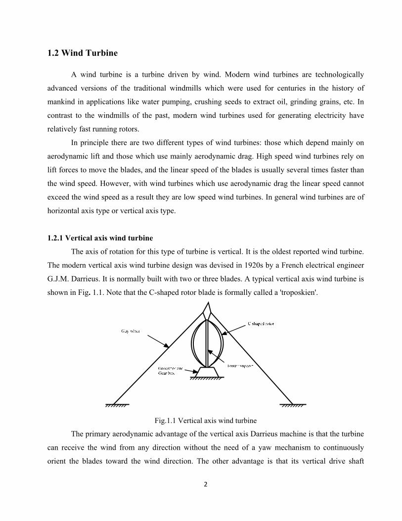
The axis of rotation for this type of turbine is vertical. It is the oldest reported wind turbine.

The modern vertical axis wind turbine design was devised in 1920s by a French electrical engineer

G.J.M. Darrieus. It is normally built with two or three blades. A typical vertical axis wind turbine is

shown in Fig. 1.1. Note that the C-shaped rotor blade is formally called a 'troposkien'.

Fig.1.1 Vertical axis wind turbine

The primary aerodynamic advantage of the vertical axis Darrieus machine is that the turbine

can receive the wind from any direction without the need of a yaw mechanism to continuously

orient the blades toward the wind direction. The other advantage is that its vertical drive shaft

3

simplifies the installation of gearbox and electrical generator on the ground, making the structure

much simpler. On the disadvantage side, it normally requires guy wires attached to the top for

support. This could limit its applications, particularly for offshore sites. Wind speeds are very low

close to ground level, so although it might save the need for a tower, the wind speed will be very

low on the lower part of the rotor. Overall, the vertical axis machine has not been widely used\

because its output power cannot be easily controlled in high winds simply by changing the pitch.

Also Darrieus wind turbines are not self-starting, however straight-bladed vertical axis wind

turbines with variable-pitch blades are able to overcome this problem.

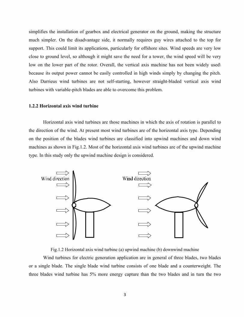
1.2.2 Horizontal axis wind turbine

Horizontal axis wind turbines are those machines in which the axis of rotation is parallel to

the direction of the wind. At present most wind turbines are of the horizontal axis type. Depending

on the position of the blades wind turbines are classified into upwind machines and down wind

machines as shown in Fig.1.2. Most of the horizontal axis wind turbines are of the upwind machine

type. In this study only the upwind machine design is considered.

Fig.1.2 Horizontal axis wind turbine (a) upwind machine (b) downwind machine

Wind turbines for electric generation application are in general of three blades, two blades

or a single blade. The single blade wind turbine consists of one blade and a counterweight. The

three blades wind turbine has 5% more energy capture than the two blades and in turn the two

4

blades has 10% more energy capture than the single blade. These figures are valid for a given set of

turbine parameters and might not be universally applicable.

The three blade wind turbine has greater dynamic stability in free yaw than two blades,

minimizing the vibrations associated with normal operation, resulting in longer life of all

components.

1.3 Power extracted from wind

Air has a mass. As wind is the movement of air, wind has a kinetic energy. To convert this

kinetic energy of the wind to electrical energy, in a wind energy conversion system, the wind

turbine captures the kinetic energy of the wind and drives the rotor of an electrical generator.

The kinetic energy (KE) in wind is given by

2

2

1mVKE (1.1)

where m- is the mass of air, in kg

V-is the speed of air, in m/s

The power in wind is calculated as the flux of kinetic energy per unit area in a given time, and can

be written as

22

2

1

2

1)(VmV

dt

dm

dt

KEdP (1.2)

where m is the mass flow rate of air per second, in kg/s, and it can be expressed in terms of the

density of air (ρ in kg/m3) and air volume flow rate per second (Q in m3/s) as given below

AVQm (1.3)

5

where A-is the area swept by the blades of the wind turbine, in m2.

Substituting equation (1.3) in (1.2), we get

3

2

1AVP (1.4)

This is the total wind power entering the wind turbine. Remember that for this to be true V

must be the wind velocity at the rotor, which is lower than the undisturbed or free stream velocity.

This calculation of power developed from a wind turbine is an idealized one-dimensional analysis

where the flow velocity is assumed to be uniform across the rotor blades, the air is incompressible

and there is no turbulence where flow is inviscid (having zero viscosity).

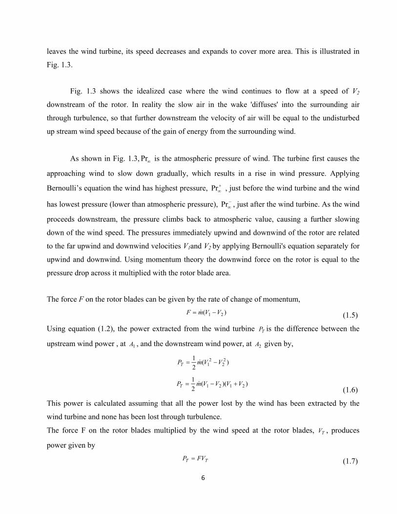
Fig.1.3 Change of wind speed and wind pressure around the wind turbine

The volume of air entering the wind turbine should be equal to the volume of air leaving the

wind turbine because there is no storage of air in the wind turbine. As a result, volume flow rate per

second, Q , remains constant, which means the product AV remains constant. Hence when the wind

rTP

rTP

6

leaves the wind turbine, its speed decreases and expands to cover more area. This is illustrated in

Fig. 1.3.

Fig. 1.3 shows the idealized case where the wind continues to flow at a speed of V2

downstream of the rotor. In reality the slow air in the wake 'diffuses' into the surrounding air

through turbulence, so that further downstream the velocity of air will be equal to the undisturbed

up stream wind speed because of the gain of energy from the surrounding wind.

As shown in Fig. 1.3, Pr is the atmospheric pressure of wind. The turbine first causes the

approaching wind to slow down gradually, which results in a rise in wind pressure. Applying

Bernoulli’s equation the wind has highest pressure, Pr , just before the wind turbine and the wind

has lowest pressure (lower than atmospheric pressure), Pr , just after the wind turbine. As the wind

proceeds downstream, the pressure climbs back to atmospheric value, causing a further slowing

down of the wind speed. The pressures immediately upwind and downwind of the rotor are related

to the far upwind and downwind velocities V1and V2 by applying Bernoulli's equation separately for

upwind and downwind. Using momentum theory the downwind force on the rotor is equal to the

pressure drop across it multiplied with the rotor blade area.

The force F on the rotor blades can be given by the rate of change of momentum,

)( 21 VVmF (1.5)

Using equation (1.2), the power extracted from the wind turbine TP is the difference between the

upstream wind power , at 1A , and the downstream wind power, at 2A given by,

)(2

1 22

21 VVmPT

))((

2

12121 VVVVmPT

(1.6)

This power is calculated assuming that all the power lost by the wind has been extracted by the

wind turbine and none has been lost through turbulence.

The force F on the rotor blades multiplied by the wind speed at the rotor blades, TV , produces

power given by

TT FVP (1.7)

7

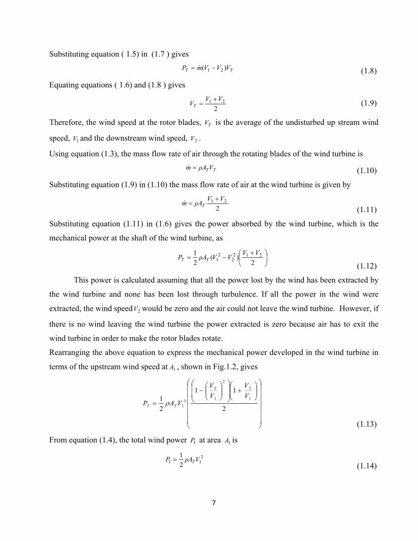
Substituting equation ( 1.5) in (1.7 ) gives

TT VVVmP )( 21 (1.8)

Equating equations ( 1.6) and (1.8 ) gives

221 VV

VT

(1.9)

Therefore, the wind speed at the rotor blades, TV is the average of the undisturbed up stream wind

speed, 1V and the downstream wind speed, 2V .

Using equation (1.3), the mass flow rate of air through the rotating blades of the wind turbine is

TTVAρm (1.10)

Substituting equation (1.9) in (1.10) the mass flow rate of air at the wind turbine is given by

221 VV

Aρm T

(1.11)

Substituting equation (1.11) in (1.6) gives the power absorbed by the wind turbine, which is the

mechanical power at the shaft of the wind turbine, as

2)(

2

1 2122

21

VVVVAρP TT

(1.12)

This power is calculated assuming that all the power lost by the wind has been extracted by

the wind turbine and none has been lost through turbulence. If all the power in the wind were

extracted, the wind speed 2V would be zero and the air could not leave the wind turbine. However, if

there is no wind leaving the wind turbine the power extracted is zero because air has to exit the

wind turbine in order to make the rotor blades rotate.

Rearranging the above equation to express the mechanical power developed in the wind turbine in

terms of the upstream wind speed at 1A , shown in Fig.1.2, gives

2

11

2

1 1

2

2

1

2

31

V

V

V

V

VAP TT

(1.13)

From equation (1.4), the total wind power 1P at area 1A is

3

11 2

1VAρP T

(1.14)

8

Then the ratio of wind power extracted by the wind turbine to the total wind power at area 1A is the

dimensionless power coefficient pC , where

2

111

22

1

2

V

V

V

V

C p (1.15)

Substituting equation (1.15) into equation (1.13) the wind power extracted by the wind turbine can

be written as

pTT CVAρP 3

12

1

(1.16)

or

pTT CVDP 3

12

8

1 (1.17)

where TD is the sweep diameter of the wind turbine.

1.4 Generators for wind power applications

Mainly the generators which are used for electricity generation from wind power are

permanent magnet synchronous generator, squirrel cage induction generator and doubly fed

induction generator.

1.4.1 Permanent Magnet Synchronous Generator

Wind turbines run at inconveniently low speeds, typically 25-50 rpm. A speed-increasing

gear box is required to run induction machines and conventional synchronous machines at 1000 or

1500 rpm for operation with the utility network. Additional cost, weight, power loss, regular

maintenance, and noise generation are some of the problems associated with the gear box. This

speed boost is necessary, as induction and synchronous machines cannot be built with pole pitches

less than 150 mm and a large number of poles in the range 120-240, necessary for the direct

coupled generator turning at low speed, cannot be accommodated within an acceptable diameter of

the generator, which should fit inside the nacelle with the gear box. Therefore, low-speed, direct-

coupled generators are required, particularly for turbines with large diameters.

9

Permanent magnet (PM) excitation considerably brings down the pole pitch requirement,

which should be less than 40 mm. This allows the rotor to be within an acceptable diameter, which

makes the housing of the generator inside the nacelle possible. In the surface-type permanent

magnet machine, high-energy, rare-earth magnets such as neodymium-iron-boron (Nd-Fe-B) are

mounted on the rotor surface. In per-unit terms, both the reactance values are small because of the

large number of poles. This provides the PMSG with high peak torque capability to resist higher-

than-rated torque for short periods during wind gusts and repeated torque pulsations of up to 20% of

the rated torque.

1.4.2 Squirrel Cage Induction Generator

The operation of a squirrel cage induction machine as a self-excited generator in isolation

with variable-speed prime movers, such as wind turbines, has poor voltage and frequency

regulation. For frequency insensitive loads, such as heating and lighting, it is adequate to maintain a

near-constant terminal voltage. In fact, irrespective of the nature and amount of load, a constant

terminal voltage with admissible regulation is required in most applications. The generated ac

voltage may either be used directly or converted into dc voltage. Dc power can be used directly in

certain dc equipment, such as battery chargers, or fed to the ac mains, or load, through an inverter.

1.4.3 Doubly Fed Induction Generator

The wound rotor induction machine, commonly known as the doubly fed induction generator, is

finding increasing application, particularly in the megawatt range, in variable-speed wind energy

conversion systems. When compared with motoring operation, the power handling capability of a

wound rotor induction machine as a generator theoretically becomes nearly double. The rotor of the

generator is coupled to the turbine shaft through a gear box so that a standard (1500/1800 rpm)

wound rotor induction machine can be used. The gear ratio is so chosen that the machine’s

synchronous speed falls nearly in the middle of the allowable speed range of the turbine (nearly 60-

110%). Above the rated wind speed, power is limited to the rated value by pitching the blades. The

stator is directly connected to the fixed-frequency utility grid while the rotor collector rings are

connected via back-to-back PWM voltage source inverters and a transformer/filter to the same

utility grid. As the rotor power is a fraction of the total power of the generator, a rotor converter

rating of nearly 35% of the rated turbine power is sufficient. The rotor-side PWM converter is a

10

stator flux based controller that provides independent control of the induction machine’s active and

reactive powers. The grid-side converter is the dc-link voltage regulator that enables power flow to

the grid, keeping the dc-link voltage level constant.

1.5 Self Excitation and Line Excitation of Induction Generator

Excitation current is responsible to magnetize the core and producing a rotating magnetic field.

The excitation current for an induction generator connected to an external source, such as the grid,

is supplied from that external source. If this induction generator is driven by a prime mover above

the synchronous speed, electrical power will be generated and supplied to the external source. An

isolated induction generator without any excitation will not generate voltage and will not be able to

supply electric power irrespective of the rotor speed. Induction generators can be classified on the

basis of excitation process as

Grid connected induction generator

Self-excited induction generator (SEIG)

In general an ac machine requires reactive power for its operation. The grid connected

induction generator takes its reactive power for excitation process from the grid supply, so it is

called grid excited induction generator. The self excited induction generators draw reactive power

from capacitors connected across its terminals.

Based on the method of excitation, induction generators are classified namely as

Constant-voltage, constant-frequency generators

Variable-voltage, variable-frequency generators

Self-excited induction generator means a cage rotor induction machine with shunt capacitors

connected at their terminals for self excitation. These are primarily variable-voltage, variable

frequency generators. Three charged capacitors connected to the stator terminals of the induction

generator can supply the reactive power required by the induction generator.

11

Depending upon the prime movers used and their locations, generating schemes can be broadly

classified as under

Constant speed constant frequency [CSCF]

Variable speed constant frequency [VSCF]

Variable speed variable frequency [VSVF]

For the voltage to build up across the terminals of the induction generator, there are certain

requirements for minimum rotor speed and capacitance value that must be met. When capacitors are

connected across the stator terminals of an induction machine, driven by an external prime mover,

voltage will be induced at its terminals. The induced emf and current in the stator windings will

continue to rise until steady state is attained. At this operating point the voltage and current will

continue to oscillate at a given peak value and frequency. The rise of the voltage and current is

influenced by the magnetic saturation of the machine. In order for self-excitation to occur with a

particular capacitance value there is a corresponding minimum speed.

Self-excited induction generators are good candidates for wind powered electricity

generation, especially in remote areas, because they do not need an external power supply to

produce the excitation magnetic field. Permanent magnet generators can also be used for wind

energy applications; however the generated voltage increases linearly with wind turbine speed. An

induction generator can cope with a small increase in speed from its rated value because, due to

saturation, the rate of increase of generated voltage is not linear with speed. Furthermore when there

is a short circuit at the terminals of the self-excited induction generator (SEIG) the voltage collapses

providing a self-protection mechanism. Additional advantages of SEIGs include lower cost,

reduced maintenance, they are rugged with simple construction, and they have a brushless rotor

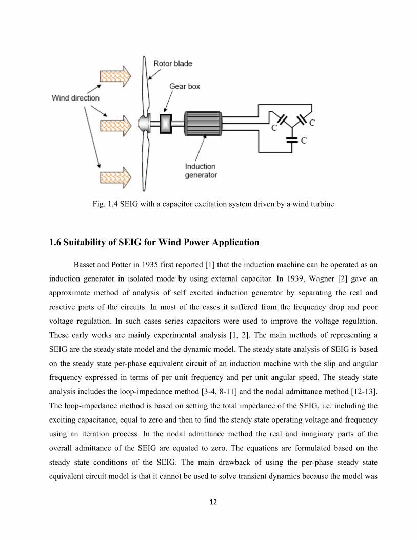
(squirrel cage). Fig. 1.4 shows the SEIG driven by a wind turbine.

12

Fig. 1.4 SEIG with a capacitor excitation system driven by a wind turbine

1.6 Suitability of SEIG for Wind Power Application

Basset and Potter in 1935 first reported [1] that the induction machine can be operated as an

induction generator in isolated mode by using external capacitor. In 1939, Wagner [2] gave an

approximate method of analysis of self excited induction generator by separating the real and

reactive parts of the circuits. In most of the cases it suffered from the frequency drop and poor

voltage regulation. In such cases series capacitors were used to improve the voltage regulation.

These early works are mainly experimental analysis [1, 2]. The main methods of representing a

SEIG are the steady state model and the dynamic model. The steady state analysis of SEIG is based

on the steady state per-phase equivalent circuit of an induction machine with the slip and angular

frequency expressed in terms of per unit frequency and per unit angular speed. The steady state

analysis includes the loop-impedance method [3-4, 8-11] and the nodal admittance method [12-13].

The loop-impedance method is based on setting the total impedance of the SEIG, i.e. including the

exciting capacitance, equal to zero and then to find the steady state operating voltage and frequency

using an iteration process. In the nodal admittance method the real and imaginary parts of the

overall admittance of the SEIG are equated to zero. The equations are formulated based on the

steady state conditions of the SEIG. The main drawback of using the per-phase steady state

equivalent circuit model is that it cannot be used to solve transient dynamics because the model was

13

derived from the steady state conditions of the induction machine. The dynamic model of a SEIG is

based on the d-q axes equivalent circuit or unified machine theory. For analysis the induction

machine in three axes is transformed to two axes, d and q, and all the analysis is done in the d-q

axes model. The results are then transformed back to the actual three axes representation. In the d-q

axes, if the time varying terms are ignored the equations represent only the steady state conditions.

The SEIG represented in d-q axes and the analyzed under steady state condition is reported in [5].

In [12, 20-21] the dynamic equations for the representation of SEIG conditions are given. In these

papers the initial conditions that take into account the initial charge in the exciting capacitors and

the remnant magnetic flux linkage in the iron core are not given. The d-q axes model of SEIG given

in [21] reported that the dynamic generated voltage varies with the applied load, but there are no

results that show what happens to the dynamic speed of the rotor when the generator is loaded.

Hence it cannot be proven that whether the variation in voltage is due to a change in speed or not.

In [15] a SEIG with electrical connection between stator and rotor windings is reported. This paper

deals with the steady state performance of a SEIG realized by a series connection of stator and rotor

windings of a slip-ring type induction machine and solved using d-q analysis. In this type of

connection it has been claimed that it has the advantage of operating at a frequency independent of

load conditions for a fixed rotor speed, however the angular frequency of the output voltage is equal

to half of the rotor electrical angular speed, which means the prime mover should rotate at twice the

normal speed to generate voltage with standard frequency. There is also concern regarding the

current carrying capability of the stator and rotor windings because both of them are carrying the

same current. If a single valued capacitor bank is connected, i.e. without voltage regulator, a SEIG

can safely supply an induction motor rated up to 50% of its own rating and with a voltage regulator

that maintains the rated terminal voltage the SEIG can safely feed an induction motor rated up to

75% of its own rating [17]. In this case the SEIG can sustain the starting transients of the induction

motor without losing self-excitation. The output voltage and frequency of an isolated induction

generator vary depending on the speed of the rotor and the load connected to the generator. This is

due to a drop in the speed of the rotating magnetic field . The wind turbine can be designed to

operate at constant speed or variable speed. When the speed of the prime mover of the isolated

induction generator drops with load, then the decrease in voltage and frequency will be greater than

for the case where the speed is held constant. The AC voltage can be compensated by varying the

exciting AC capacitors or using a controlled inverter and a DC capacitor. However the frequency

14

can be compensated only if there is a change in the rotor speed. Because the frequency of the three-

phase isolated induction generator varies with loading, its application should be for the supply of

equipment insensitive to frequency deviations, such as heaters, water pumps, lighting, battery

charging etc. Dynamic performance of self excited induction generator feeding different static loads

is mentioned in [31].A nonlinear dynamic model is proposed in [38] along with the explanation of

the experimental data. This theory takes into account the demerits of linear theory which could not

account for slower growth of terminal voltage than exponential growth and for sustained sinusoidal

oscillations for many cycles before collapsing. The performance of an isolated self excited

induction generator driven by a wind turbine under unbalanced loads is studied in [39]. In this paper

the whole system, including the induction generator, the capacitors and the loads is modeled using

park transformation allowing saturation effect into account. Magnitude and frequency of the

voltages are found to be less affected even if the load is unbalanced.

1.6.1 Capacitance and rotor speed for self-excitation

The minimum and maximum values of capacitance required for self-excitation of a three-

phase induction generator have been analyzed using a current model [8,10,21]. Calculation of the

minimum capacitance required for self excitation using a flux model has also been reported in [23].

In the calculation of capacitance required for self-excitation, economically and technically, it is not

advisable to choose the maximum value of capacitance. This is due to the fact that for the same

voltage rating the higher capacitance value will cost more. In addition, if the higher capacitance

value is chosen then there is a possibility that the current flowing in the capacitor might exceed the

rated current of the stator due to the fact that the capacitive reactance reduces as the capacitance

value increases. A de-excited induction generator can re-excite even if the load is already connected

to it [18]. Wind speed can change from the minimum set point to the maximum set point randomly

and the SEIG can be started at any point within the range of speed. It is essential to find the

minimum and maximum speed required for self-excitation, when the generator is loaded. In [30]

the author has presented the analysis and calculation of the minimum and maximum speeds for self

excitation to occur and for a particular value of capacitance.

15

1.6.2Effect of magnetizing inductance on self-excitation

In the SEIG the variation of magnetizing inductance is the main factor in the dynamics of

voltage build up and stabilization. Effect of variation of magnetizing inductance or magnetizing

reactance during voltage build up has been reported in several papers. In [3-4, 8, 10-11, 13] the

effect of magnetizing reactance on voltage build up is reported and the effect of magnetizing

inductance for a known frequency of operation is reported in [12,16]. In these papers it has been

shown that as the air gap voltage increases from zero, the value of magnetizing reactance starts at a

given unsaturated value reaches a peak value than starts to decrease up to its rated value, which is a

saturated value. In these analyses of the SEIG the magnetizing reactance for values of air gap

voltage close to zero were ignored. Since magnetizing reactance is dependent on frequency it is

avoided in transient analysis, rather magnetizing inductance is used. In [5,18,21,24] it has been

shown that the magnetizing inductance or magnetizing reactance starts at a maximum unsaturated

value and then decreases when the iron core saturates. Although this representation depicts the

actual variation of magnetizing inductance, the significance of this characteristic has not been

presented.

1.6.3 Control of generated voltage and frequency

The main problem in using a SEIG is the control of the generated voltage because the

voltage amplitude and frequency drops with loading as well as with a decrease in the generator

rotor speed [29]. For applications that require constant voltage and frequency the rectified DC

voltage of the isolated induction generator should be controlled to remain at a given reference

value. Then the constant DC voltage can be converted to constant AC voltage and frequency using

an output inverter. In this way a control mechanism is implemented to regulate the output voltage

and frequency from an induction generator. The generated voltage can be controlled by varying the

rotor resistance of a self- excited slip-ring induction generator [28]. However a self-excited slip-ring

induction generator will require more maintenance than a squirrel cage rotor due to the slip-rings

and brush gear. The rms value of the generated voltage, irrespective of its frequency, can be

controlled using variable capacitance values [6], or a fixed capacitor thyristor controlled reactor

static VAR compensator [26], or continuously controlled shunt capacitors using anti-parallel IGBT

switches across the excitation capacitor [22]. In a SEIG, a squirrel cage rotor is preferable to a

wound rotor because the squirrel cage rotor has a higher thermal withstand capability and requires

16

less maintenance. Due to the higher thermal withstand capability of the squirrel cage rotor, a higher

copper loss in the rotor is acceptable.

Maintaining a constant frequency is not a problem for a fixed speed wind turbine system

connected to the grid. However the problem is with the operation of SEIG. A stand-alone induction

generator excited by a single DC capacitor and inverter/rectifier system can be used instead of the

AC capacitor excited system. If a constant DC voltage is achieved then a load side inverter is used

to produce a constant rms voltage and frequency. An inverter/rectifier can be shunt connected so

that it carries only the exciting current or a converter can be connected in series so that it carries the

full current, i.e. the exciting and load current [14,19,25,27]. A novel voltage controller for

standalone induction generator using PWM-VSI is reported in [32]. In this paper speed was not

taken into account but three phase reference voltage signal is generated considering the error output

of the PI controller as synchronous frequency. The error input is generated by comparing the DC

link capacitor voltage with the reference DC voltage. A similar but with a frequency control scheme

is depicted in [33]. Both of these above two papers uses scalar control technique. A vector control

scheme taking saturation effect into account is explained in [34]. The constant voltage operation of

SEIG using optimization tools such as genetic algorithm, pattern search and quasi-newton is

mentioned in [35]. A DSP based load controller for a single phase SEIG is described in [36]. A

detailed vector control scheme using a hysteresis controller for constant voltage and frequency

controller is reported in [37].The above papers did not mention the effect of speed, excitation

capacitance, mutual inductance on dynamic power variations and frequency of power exchange and

line voltage.

1.7 Motivation and Objectives

1.7.1 Motivation

The continuously increasing energy demand has forced researchers in the energy area to go

for alternative solutions to non renewable resources. Non renewable resources on the other hand is

also limited and in the depleting mode. Humanity has also witnessed deep environmental hazards

from non renewable sources in the recent past. The previous works of researchers in harnessing the

clean renewable energy like wind, hydro, tidal, solar, biomass for electric power generation is the

prime motivation to take up this project as a first step towards understanding the technology in the

renewable energy sector. Though the induction generator self excitation phenomena is known since

17

1935, till date the work in the area of dynamic analysis, steady state analysis and control of voltage,

frequency is a concern. The usefulness of an isolated induction generator is many fold especially

where extension of national grid is not feasible or economical. The conversion of an already

existing induction motor to an isolated induction generator locally by suitable technology transfer to

the masses is the focus of this project.

1.7.2 Objectives

To model the induction machine as a self excited induction generator taking dynamic

mutual inductance into consideration by including both R and RL loads.

To analyze the effect of speed, excitation capacitance and mutual inductance on

dynamic power variations and frequency of power exchange and line voltage.

Simulating a voltage control scheme to extract the information on active power and

reactive power and torque variations under no load and loaded conditions.

To analyze the effect of proportional gain of PI controller on the shape of line

current and on its frequency.

To experimentally verify the operation of a three phase induction machine as a self

excited induction generator by including a capacitor bank in delta connected mode

for the necessary reactive power supply.

1.8 Scope and Organization of the Thesis

There are six chapters in this thesis. The thesis presents the voltage control of self excited

induction generator along with its modeling and analysis, when driven by a wind turbine. To have a

good understanding of the prime mover an overview of the characteristics of wind turbines is

presented. Analysis of an induction generator is done using d-q modeling and the theory of

induction machines.

In Section 1.6 of this chapter the literature related to isolated induction generators is

reviewed. This involves clarifying the strengths and limitations of the previous works and

highlighting the advantages of the research covered in the thesis.

18

In Chapter 2 reference frame theory and the induction machine modeling are presented. In

electrical machine analysis a three-axes to two-axes transformation is applied to produce simpler

expressions that provide more insight into the interaction of the different parameters. The d-q model

for dynamic analysis is obtained using this transformation. It is shown that the three-axes to two-

axes transformation reduces the no. of equations to solve, simplifies the calculation of dynamic rms

current, rms voltage, active power for the three-phase induction machine. The modeling of an

induction machine using the conventional or steady state model and the d-q or dynamic model are

explained. The voltage, current and flux linkage in the rotating reference frame and their phase

relationships in the motoring region and generating region are presented. This chapter describes the

fundamentals of induction machine modeling and characteristics as a preparation of the modeling

and analysis of an isolated induction generator. Using this model the dynamic current, torque and

power can be calculated more accurately.

Chapter 3 deals with the modeling and analysis of an isolated three-phase induction

generator excited by three AC capacitors connected at the stator terminals. The mathematical model

of a self-excited induction generator and the initial charge in the capacitor is given. The initiation

and process of self-excitation is presented, starting from a simple RLC circuit as an analogy to a

complete dynamic representation of a self-excited induction generator, i.e. the complete

representation includes both steady state and transient conditions. The variation of magnetizing

inductance of the induction machine is important in the voltage build up and stabilization of the

generated voltage. It is shown that the characteristics of magnetizing inductance with respect to the

rms induced stator voltage or magnetizing current determines the regions of stable operation as well

as the minimum generated voltage without loss of self-excitation. The variation of the generated

voltage for a self excited induction generator at constant and variable speeds for varying excitation

capacitors has been investigated. More results which are not accessible in an experimental setup

have been analyzed using simulation algorithms.

In Chapter 4 the terminal voltage control in an isolated induction generator using an

inverter/rectifier excitation with a single capacitor on the DC link is discussed. A scalar control

technique is verified to control the excitation and the reactive power. When the speed of the prime

mover is varied, the flux linkage in the induction generator is made to vary inversely proportional to

19

the rotor speed so that the generated voltage remains constant. The first scheme controls only the

terminal voltage by keeping the modulation index fixed. The second scheme controls both terminal

voltage and frequency by varying the modulation index as a part of control. Both the scheme use a

single PI controller.

Chapter 5 presents the experimental verification of an induction machine being run as a self

excited induction generator using a capacitor bank of three power capacitors in delta connection.

Open circuit test and short circuit test are performed to find the machine parameters. The

magnetization characteristic curve of an induction machine was found by running it at synchronous

speed.

In Chapter 6 conclusions and suggestions for future work are given.

Major Contributions in the thesis are :

Review of d-q axes modeling of induction generator.

Mathematical analysis of self excited induction generator.

Analysis of effects of speed, excitation capacitance and mutual inductance on self

excitation process of induction generator.

Simulation of self excited induction generator with R-L load.

Design and analysis of a closed loop voltage control scheme for SEIG.

Simulation and analysis of closed loop voltage control scheme.

Experiments on voltage build-up of SEIG.

20

CHAPTER 2

REFERENCE FRAME THEORY AND INDUCTION

MACHINE MODELLING

2.1 Introduction

The dynamic performance of an induction machine is somewhat complex because the three-

phase rotor windings move with respect to the three-phase stator windings. This machine can be

studied as a transformer with a moving secondary, where the coupling coefficients between the

stator and rotor phases change continuously with the change of rotor position r since machine

model can be described by differential equations with time-varying mutual inductances, but such a

model is very complex. More conveniently, a three phase machine can be represented by an

equivalent two-phase machine making the analysis simpler, but the problem of time varying

parameters is a subject of concern.

Some of the reference frame transformations proposed in this approach are as follows.

-R.H.Park, in the 1920s formulated a change of variables, which, in effect, replaced the variables

(Voltages, currents, and flux linkages) associated with the stator windings of a synchronous

machine with variables associated with fictitious windings rotating with the rotor at synchronous

speed. He transformed the stator variables to a synchronously rotating reference frame fixed in the

rotor. All the time-varying inductances that occur due to an electric circuit in relative motion, and

electric circuits with varying magnetic reluctances were eliminated.

21

-By transforming the rotor variables to variables associated with fictitious stationary windings, time

varying inductances in the voltage equation of an induction machine due to electric circuits in

relative motion can be eliminated. This was proposed by H.C. Stanley in the late 1930s.

-G. Kron proposed a change of variables which eliminated the time-varying inductances of a

symmetrical induction machine by transforming both the stator variables and the rotor variables to a

reference frame rotating in synchronism with the rotating magnetic field. This reference frame is

commonly referred to as the synchronously rotating reference frame.

-Transformation of stator variables to a rotating reference frame that is fixed in the rotor was

proposed by D. S. Brereton. This is essentially Park’s transformation applied to induction machines.

In 1965, Krause and Thomas have shown that time-varying inductances can be eliminated by

referring the stator and rotor variables to a common reference frame which may rotate at any speed

(arbitrary reference frame).

In this chapter, first transformation from a three phase system to a 2-phase stationary, ds-qs

reference frame is reviewed. Then transformation from 2-phase stationary, ds-qs to synchronously

rotating de-qe reference frame is reviewed. Power balance during reference frame transformations is

carefully studied. Then the equations governing induction machine dynamics in the stationary

reference frame and corresponding d-axis and q-axis equivalent circuits are presented. After that,

the induction machine model in synchronously rotating reference and corresponding d-axis and q-

axis equivalent circuits are discussed.

2.2 Reference Frame Transformations

The three axes are representing the real three phase supply system. However, the two axes

are fictitious axes representing two fictitious phases perpendicular to each other. The transformation

of three-axes to two-axes can be done in such a way that the two-axes are in a stationary reference

frame, or in rotating reference frame. If the reference frame is rotating at the same angular speed as

the excitation frequency, when the variables are transformed into this rotating reference frame, they

will appear as constant dc values instead of time varying quantities.

22

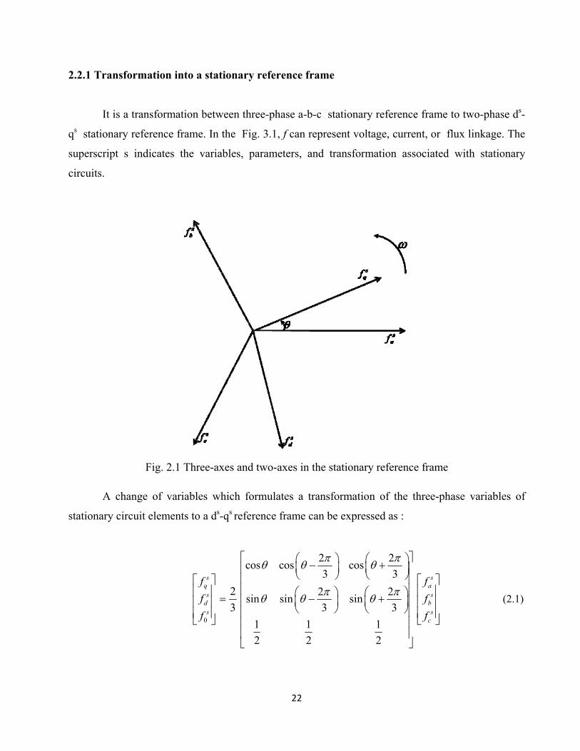
2.2.1 Transformation into a stationary reference frame

It is a transformation between three-phase a-b-c stationary reference frame to two-phase ds-

qs stationary reference frame. In the Fig. 3.1, f can represent voltage, current, or flux linkage. The

superscript s indicates the variables, parameters, and transformation associated with stationary

circuits.

Fig. 2.1 Three-axes and two-axes in the stationary reference frame

A change of variables which formulates a transformation of the three-phase variables of

stationary circuit elements to a ds-qs reference frame can be expressed as :

0

sqs

ds

f

f

f

2

3

2 2cos cos cos

3 3

2 2sin sin sin

3 3

1 1 1

2 2 2

sas

bs

c

f

f

f

(2.1)

23

In equation (2.1) sf0 is a variable that takes care of the unbalance in the variables of the

three-axes system and is the same as the zero-sequence component in three phase system. It is

important to note that the zero-sequence variables are not associated with the reference frame.

Instead, the zero-sequence variables are related arithmetically to the abc variables, independent of

θ.

saf , s

bf ,and scf are instantaneous quantities, which maybe any function of time. Portraying the

transformation, as shown in Fig. 2.1, is particularly convenient when applying it to ac machines

where the direction of saf , s

bf ,and scf may also be thought of as the direction of the magnetic axes

of the stator windings. They can also represent space vectors or the axes of distribution of the phase

windings. The direction of sqf and s

df can be considered as the direction of the magnetic axes of

the new windings created by the change of variables.

The inverse of equation (2.1), which can be derived directly from the relationship givenin Fig. 2.1,

is

sas

bs

c

f

f

f

cos sin 1

2 2cos sin 1

3 3

2 2cos sin 1

3 3

0

sqs

ds

f

f

f

(2.2)

In Fig. 2.1, if the q-axis is aligned with the a-axis, i.e. 0 , equation (2.1) will be written as:

0

sqs

ds

f

f

f

2

3

1 11

2 2

3 30

2 21 1 1

2 2 2

sas

bs

c

f

f

f

(2.3)

24

and equation (2.2) will be simplified to:

sas

bs

c

f

f

f

1 0 1

1 31

2 2

1 31

2 2

0

sqs

ds

f

f

f

(2.4)

In equations (2.3) and (2.4) the magnitude of the phase quantities, voltages and currents, in

the three ( )abc axes and two ( )dq axes remain the same. This transformation is based on the

assumption that the number of turns of the windings in each phase of the three axes and the two

axes are the same. Here the advantage is the peak values of phase voltages and phase currents

before and after transformation remain the same.

2.2.2 Transformation into a rotating reference frame

The rotating reference frame can have any speed of rotation depending on the choice of the

user. Selecting the excitation angular frequency as the speed of the rotating reference frame gives

the advantage that the transformed variables, appear as constant (DC) values. In other words, an

observer moving along at that same speed will see the space vector as a constant spatial

distribution, unlike the time-varying values in the stationary abc axes.

In the previous section the transformation from a-b-c axes to a stationary ds-qs axes is

given. Here the stationary ds-qs axes will be transformed into a rotating de-qe reference frame, which

is rotating at e , excitation frequency.

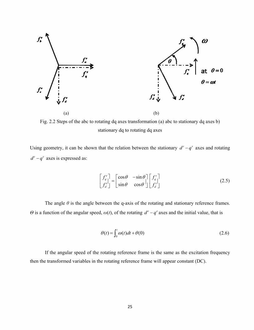
Fig. 2.2 shows the abc to rotating de-qe transformation in two steps, i.e, first transforming to

stationary ds-qs axes and then to rotating de-qe axes.

25

(a) (b)

Fig. 2.2 Steps of the abc to rotating dq axes transformation (a) abc to stationary dq axes b)

stationary dq to rotating dq axes

Using geometry, it can be shown that the relation between the stationary s sd q axes and rotating

e ed q axes is expressed as:

eqe

d

f

f

cos sin

sin cos

sqs

d

f

f

(2.5)

The angle θ is the angle between the q-axis of the rotating and stationary reference frames.

Θ is a function of the angular speed, ω(t), of the rotating e ed q axes and the initial value, that is

0( ) ( ) (0)

tt t dt (2.6)

If the angular speed of the rotating reference frame is the same as the excitation frequency

then the transformed variables in the rotating reference frame will appear constant (DC).

26

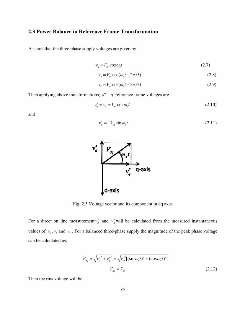
2.3 Power Balance in Reference Frame Transformation

Assume that the three phase supply voltages are given by

cosa m ev V t (2.7)

cos( 2 3)b m ev V t (2.8)

cos( 2 3)c m ev V t (2.9)

Then applying above transformations; s sd q reference frame voltages are

coss

q a m ev v V t (2.10)

and

sinsd m ev V t (2.11)

Fig. 2.3 Voltage vector and its component in dq axes

For a direct on line measurement sdv and s

qv will be calculated from the measured instantaneous

values of av , bv and cv . For a balanced three-phase supply the magnitude of the peak phase voltage

can be calculated as:

dqV 2 2s sd qv v 2 2 2[(sin ) (cos ) ]m e eV t t

dq mV V (2.12)

Then the rms voltage will be

27

2dq

rms

VV (2.13)

Similarly, the three phase currents flowing in the system may be described as

cos( )a m ei I t (2.14)

cos( 2 3 )b m ei I t (2.15)

cos( 2 3 )c m ei I t (2.16)

Through the 3-phase to 2-phase ds-qs transformation:

cos( )s

q m ei I t (2.17)

sin( )sd m ei I t (2.18)

The magnitude of dqI can be calculated as

2 2s s

dq d qI i i

2 2 2[(sin( )) (cos( )) ]dq m e eI I t t

dq mI I (2.19)

The currents in the stationary ds-qs axes can be shown as in Fig. 2.4.

Fig. 2.4 Current vector and its component in stationary dq axes

28

Since the magnitude of dqI is equal to mI and is the same as the peak magnitude of phase

current in the abc-axes, the rms current can be evaluated from the instantaneous values in the ds-qs

axes. Therefore using Equation (2.19)

2dq

rms

II (2.20)

In three-phase three-wire system, only two phase currents ( ai and bi )are required to be measured.

The third one ( ci ) can be derived from the fact that the three-phase currents add to a total of zero.

Taking one sample of instantaneous values of currents flowing in any two phases of a three-phase

system, the rms and the peak currents of the three-phase system can be obtained instantaneously.

The transformation from three axes to two axes is done based on the concept that the peak

values of the voltages and currents in three axes as well as two axes are the same. The total power

in the system under consideration should remain the same regardless of the choice of reference

frame.

Since the voltages and currents in the three axes have the same peak values as those in the

two axes, the power in the two-axes system should be multiplied by a factor 3/2 so that the

transformation will keep the value of total power the same.

Fig. 2.5 shows the voltage and current vectors with their components in the stationary dq-

axes. Once the components of the currents and voltages are calculated in the d and q axes then

power is evaluated as

3( )

2s s s sd d q qP i v i v (2.21a)

If the currents and voltages are substituted in equation (2.21a) with the expressions given in

the voltage and current measurement sections then the classical power expression becomes

29

3cos

2 m mP I V (2.21b)

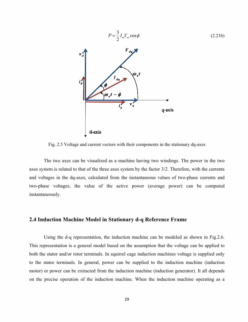
Fig. 2.5 Voltage and current vectors with their components in the stationary dq-axes

The two axes can be visualized as a machine having two windings. The power in the two

axes system is related to that of the three axes system by the factor 3/2. Therefore, with the currents

and voltages in the dq-axes, calculated from the instantaneous values of two-phase currents and

two-phase voltages, the value of the active power (average power) can be computed

instantaneously.

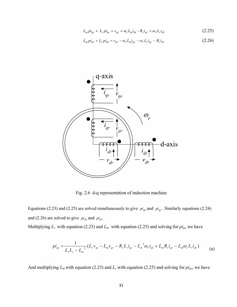
2.4 Induction Machine Model in Stationary d-q Reference Frame

Using the d-q representation, the induction machine can be modeled as shown in Fig.2.6.

This representation is a general model based on the assumption that the voltage can be applied to

both the stator and/or rotor terminals. In squirrel cage induction machines voltage is supplied only

to the stator terminals. In general, power can be supplied to the induction machine (induction

motor) or power can be extracted from the induction machine (induction generator). It all depends

on the precise operation of the induction machine. When the induction machine operating as a

30

generator is connected to the grid and driven by an external prime mover, then the rotor should be

driven above synchronous speed.

When the machine is operated as a motor, power flows from the stator to the rotor, crossing

the air gap. However, in the generating mode of operation, power flows from the rotor to the stator.

Only these two modes of operation are dealt with in this investigation. The braking region, where

the rotor rotates opposite to the direction of the rotating magnetic field, is not dealt with here.

The advantage of the d q axes model is that it is powerful for analyzing the transient and

steady state conditions, giving the complete solution of any dynamics. The general equations for the

d q representation of an induction machine, in the stationary reference frame, are given as :

qs

ds

qr

dr

v

v

v

v

0 0

0 0s s m

s s m

m r m r r r r

r m m r r r r

R pL pL

R pL pL

pL L R pL L

L pL L R pL

qs

ds

qr

dr

i

i

i

i

(2.22)

where sR - stator winding resistance,

rR - rotor winding resistance,

mL - magnetizing inductance, H

sL - stator leakage inductance )( lsL + magnetizing inductance )( mL , H

rL - rotor leakage inductance )( lrL + magnetizing inductance )( mL , H

r - electrical rotor angular speed in rad/sec and dtdp , the differential operator.

Equation (2.22) can be solved to form a matrix of first order differential equation as follows:

qss piL qrm piL qssqs iRv (2.23)

dss piL drm piL dssds iRv (2.24)

31

qsm piL qrr piL dsmrqr iLv drrrqrr iLiR (2.25)

drrdsm piLpiL drrqrrrqsmrdr iRiLiLv (2.26)

Fig. 2.6 d-q representation of induction machine

Equations (2.23) and (2.25) are solved simultaneously to give qspi and qrpi . Similarly equations (2.24)

and (2.26) are solved to give dspi and drpi .

Multiplying Lr with equation (2.23) and Lm with equation (2.25) and solving for piqs, we have

)(1 2

2 drrrmqrrmdsrmqsrsqrmqsr

mrs

qs iLLiRLiLiLRvLvLLLL

pi

(a)

And multiplying Lm with equation (2.23) and Ls with equation (2.25) and solving for piqr, we have

32

(1

2mrs

qrLLL

pi

)drrrsqrrsdsmrsqssmqrsqsm iLLiRLiLLiRLvLvL (b)

Next, equation (2.24) and equation (2.26) will be solved simultaneously as follows,

Multiplying Lr with equation (2.24) and Lm with equation (2.26) and solving for pids, we have

(1

2mrs

dsLLL

pi

)2drrmqrrrmdssrqsrmdrmdsr iRLiLLiRLiLvLvL

(c)

And multiplying Lm with equation (2.24) and Ls with equation (2.26) and solving for pidr, we have

(1

2mrs

drLLL

pi

)drrsqrrrsdssmqsmrsdrsdsm iRLiLLiRLiLLvLvL (d)

Rewriting equations (a), (b), (c) and (d) in a matrix form by taking L=LsLr – Lm2,

the first order differential equations can be written in a matrix form as follows:

dr

qr

ds

qs

pi

pi

pi

pi

L

1

sm

sm

mr

mr

L0L0

0L0L

L0L0

0L0L

dr

qr

ds

qs

v

v

v

v

L

1

rsrrssmmrs

rrsrsmrssm

rmrrmssrm

rrmrmrmsr

RLLLRLLL

LLRLLLRL

RLLLRLL

LLRLLRL

2

2

dr

qr

ds

qs

i

i

i

i

(2.27)

where 2s r mL L L L .

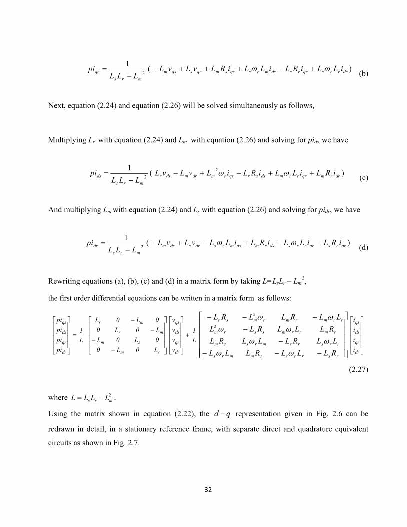
Using the matrix shown in equation (2.22), the d q representation given in Fig. 2.6 can be

redrawn in detail, in a stationary reference frame, with separate direct and quadrature equivalent

circuits as shown in Fig. 2.7.

33

(a)

(b)

Fig. 2.7 Detailed d-q representation of induction machine in stationary reference frame

(a) d-axis reference frame (b) q-axis reference frame

From the stator side (for simplicity the superscript “s” which indicates stationary reference frame is

not included with the currents, voltages and flux linkages)

ds s ds m drL i L i (2.28)

qs s qs m qrL i L i (2.29)

qrr λω

mL

dmidsi dri

dsλ drλ

sR rRlsL lrL

dsv drv

drr λω

mL

qmiqsi qri

qsλ qrλ

sR rRlsL lrL

qsv qrv

34

dsv dss ds

dR i

dt

(2.30)

qsv qss qs

dR i

dt

(2.31)

From the rotor side

dr m ds r drL i L i (2.32)

qr m qs r qrL i L i (2.33)

drv drr dr r qr

dR i

dt

(2.34)

qrv qrr qr r dr

dR i

dt

(2.35)

For the air gap flux linkage

drmdsmdmmdm iLiLiL (2.36)

qrmqsmqmmqm iLiLiL (2.37)

The stator electrical input power to the induction machine during motoring operation or the stator

electrical output power in generating mode is given by

3( )

2e ds ds qs qsP i v i v (2.38)

The electromagnetic torque eT generated by the induction machine is given by [6]

3

2e P m rT P I

(2.39)

where m

= air gap flux linkage

rI

= rotor current space vector

PP = number of pole pairs of the induction machine.

35

Solving the cross product in equation (2.39) gives

3( )

2e P m qs dr ds qrT P L i i i i (2.40)

The mechanical equation in the motoring region is

me m m

dT J D T

dt

(2.41)

and in the generating region it is given as

mm e

dT J D T

dt

(2.42)

where mT = mechanical torque in the shaft, Nm

eT = electromagnetic torque, Nm

m = mechanical shaft speed )( Prm P rad/sec

D = friction coefficient, Nm/rad/sec

J = Inertia, Kg-m2.

The mechanical power generated during motoring or the mechanical power required to drive the

induction generator is given by

m e mP T (2.43)

2.5 Induction Machine Model in Rotating d-q Reference Frame

The transformation of currents and voltages to a rotating reference frame gives a

characteristic from a different perspective. The speed of the rotating reference frame can have any

value. If the reference frame is rotating exactly at the excitation frequency then the difference

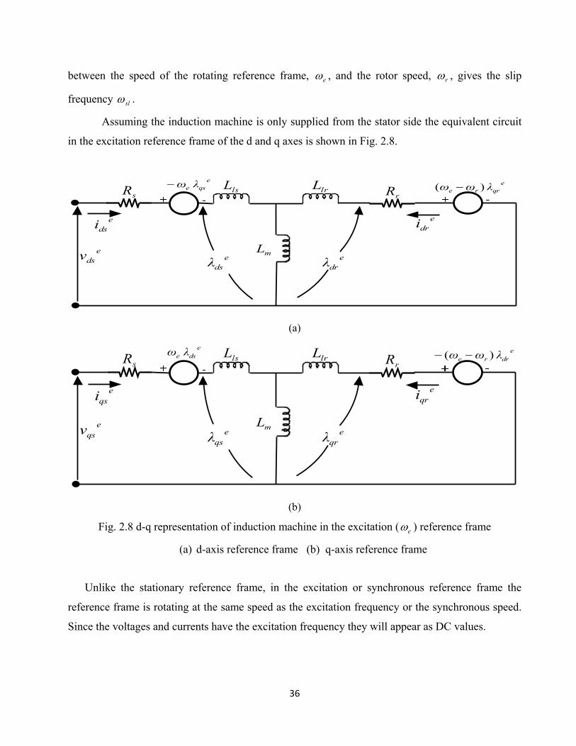
36

between the speed of the rotating reference frame, e , and the rotor speed, r , gives the slip

frequency sl .

Assuming the induction machine is only supplied from the stator side the equivalent circuit

in the excitation reference frame of the d and q axes is shown in Fig. 2.8.

(a)

(b)

Fig. 2.8 d-q representation of induction machine in the excitation ( e ) reference frame

(a) d-axis reference frame (b) q-axis reference frame

Unlike the stationary reference frame, in the excitation or synchronous reference frame the

reference frame is rotating at the same speed as the excitation frequency or the synchronous speed.

Since the voltages and currents have the excitation frequency they will appear as DC values.

eqrre λωω )(

mL

edri

edsλ

edrλ

sR rRlsL lrL

edsv

eqse λω

edsi

edrre λωω )(

mL

eqri

eqsλ

eqrλ

sR rRlsL lrL

eqsv

edse λω

eqsi

37

2.6 Conclusion

The three-axes to two-axes transformation and vice-versa are discussed in this chapter. It is

shown that the three-axes to two-axes transformation simplifies all the computations including the

calculation of rms current, rms voltage, and active power in a three-phase system. The modeling of

an induction machine using the d-q or dynamic model is explained in detail. The voltage, current

and flux linkage in the reference frame and their phase relationships in the motoring region and

generating region are presented.

38

CHAPTER 3

TRANSIENT ANALYSIS OF A SELF EXCITED

INDUCTION GENERATOR

3.1 Introduction

In the previous chapter, reference frame transformations and induction machine model in 2-

axis stationary, ds-qs reference frame and 2-axis synchronously rotating de-qe reference frame were

discussed. In this chapter, detailed study of self excitation process in induction generator is studied.

In section 3.2, self excitation process in R-L-C series circuit is described with reference to the

characteristic roots. The process of terminal voltage build-up in self excited induction generator

(SEIG) is also discussed in detail in this section. d-q axis model of SEIG is presented in section 3.3.

Mathematical conditions for self excitation in induction generator is derived in section 3.4. In

section 3.5, minimum capacitance and speed requirements for self excitation are derived. Dynamic

d-q axis model of SEIG with R-L load is discussed in section 3.6. Finally detailed study with

simulation results and discussions are presented in section 3.7.

3.2 Process of self-excitation

Whether it is a wound rotor induction machine or a squirrel cage induction machine voltage

will develop across the capacitors connected to the stator terminals when the rotor of the induction

machine is driven by an external prime mover. The voltage developed across the capacitors is the

terminal voltage of the self-excited induction generator.

39

3.2.1 RLC circuit characteristics

The behavior and analysis of the self-excited induction generator is similar to an RLC

circuit. Since the equations in the induction generator are complex, the principle of self excitation

process will be explained first using a simple RLC circuit. For analysis purpose the RLC circuit

given in Fig. 3.1 will be considered. The plus sign at the capacitor is the polarity for the initial

capacitor voltage.

Fig. 3.1 RLC circuit

Energy may be stored in an inductor or in a capacitor. A resistor is incapable of energy

storage. Switch S in Fig. 3.1 is closed at 0t . In general the two initial conditions at 0t are:

current might have been flowing in the inductor (provided that the inductor was part of another

circuit, not shown in Fig. 3.1, before 0t ) or initial voltage exists in the capacitor. If all initial

conditions are zero then there will not be any transient or steady state current flow.

In Fig. 3.1 assume that at the instant the switch is closed, the current is zero and the voltage across

the capacitor is 0cc Vv . When the switch is closed, the voltage equation in the RLC circuit is

given by

idt

Cdt

diLRi

1 coV 0 (3.1)

coV

)(ti

40

Introducing the p operator for dtd equation (3.1) can be rewritten as

pCpLR

1)(ti coV (3.2)

Then )(ti can be expressed as

)(ti CpRLp

pVco

12 (3.3)

If the denominator of equation (3.3) is equated to zero, then

CpRLp 12 0 (3.4)

Equation (3.4) is called the characteristic equation because it contains the information about the

behavior of the resulting current. The roots of the characteristic equation are

1p L

R

2

LCL

R 1

2

2

and 2p L

R

2

LCL

R 1

2

2

(3.5)

Using the roots given in Equation (3.5) the complete solution for the current expression in Equation

(3.3) is

)(ti tptp eAeA 2121 (3.6)

where 1A and 2A are determined from the initial conditions and circuit parameters, and 1p and 2p are

determined from the values of the circuit parameters R , L , and C . If the voltage across the

capacitor )(tvc is the output voltage of interest then coc VidtC

tv 1

)( .

In equation (3.5), if LCL

R 1

2

2

then the roots 1p and 2p of equation (3.6) are complex

quantities which can be expressed as jp 1 and jp 2 . Relating these expressions with

equation (3.5), the real part of the roots, , is always negative provided the resistance R is positive.

41

As a result with positive R there will be a decaying oscillation. represents the rate at which the

transient decays and , the imaginary part of the roots, represents the frequency of oscillation. In

passive circuits, like the RLC circuit mentioned above, all transient solutions have negative ,

meaning that the transient is reducing in magnitude with the progression of time and finally decays

to zero. However, if is positive, this implies that the transient is growing with the progression of

time, and in theory would increase to infinity. can be positive only if the resistance R is negative.

Negative resistance implies a power source whereas positive resistance implies a power sink. Fig.

3.2 shows the current in the RLC circuit when L 0.1H, C 100µF, 0cV -10V and the

magnitude of resistance R is 1.2Ω with positive value in Fig. 3.2(a) and negative value in Fig.

3.2(b). Close to 0t the magnitude of the instantaneous current flowing in the RLC circuit in both

cases is the same.

(a) (b)

Fig. 3.2 Current in series RLC circuit (a) for R=1.2Ω and (b) for R=-1.2Ω

Transients which grow in magnitude as shown in Fig. 3.2(b), with a positive value of , are

very rare. There is no variation in any of the values of R , L or C and as a result the current keeps

on growing. Any current flowing in a circuit dissipates power in the circuit resistance. If there is an

increasing current that dissipates increasing power, there must be some energy source available to

42

supply the increasing power. This is in fact the case in the self-excited induction generator. The

example above of a very rare transient is characteristic of a SEIG where the power source is a

prime mover.

3.2.2 Buildup of terminal voltage in SEIG

The process of voltage build-up is explained below:

For any speed of the rotor, the residual flux generates a small synchronous emf Er. The steady state

magnitude of the current through the LmC circuit is such that the voltage difference between the

synchronous saturation curve (voltage across across Lm) and the capacitor load line , at this value

of the stator current equals Er. At this stage, the slip ‘s’ being zero for no speed difference between

the rotor and the air-gap flux, no induced rotor current flows and the machine operates as a

synchronous generator.

If Er is less than Er1, the machine operates in the stable steady state in the synchronous

mode over the region oa. An increase in I in this region demands more synchronous voltage than

the residual emf Er. Consequently, the increased I is not sustained and the current comes back to its

original value. By the same reasoning, if Er is between Er1 and Er2, a stable synchronous mode of

operation is observed over the region cd. For Er≥ Er2,, stable synchronous operation takes place

from the point f onward. The regions ac and df are unstable, where, for the residual emf equal to

Er1, or Er2, the machine terminal voltage rises owing to synchronous self excitation, before entering

the next stable region. In the stable regions, the machine operates as a self-excited synchronous

generator.

43

Fig. 3.3 Modified circuit model with speed emf in the rotor circuit

Fig.3.4 Building up of voltage in a self excited induction generator (a) capacitor load line and the

saturation curve, (b) the difference between them

The possibility of a change over from synchronous generator operation to the self excited

asynchronous generator mode occurs in the region where the saturation curve emf is greater than

the capacitor voltage. While the machine operates in the synchronous mode, any disturbance

initiates an oscillation in the LC resonance circuit formed by the machine terminal capacitance and

the magnetizing inductance at the natural angular frequency CLω mn 1 . Only at the points b and

44

e does nω equal the synchronous frequency 1ω . Between the points b and e, the synchronous

inductive reactance is greater than the capacitive reactance. Hence the natural frequency wn of

oscillation is lower than the rotational (i.e., *synchronous) frequency 1ω . The air-gap flux

associated with the oscillating current rotates at a speed lower than that of the rotor, implying a

negative value of the slip. The corresponding rotational emf E(1-s), which exceeds E, drives a

current into the stator circuit, building up the terminal voltage.

The machine now enters the asynchronous generating mode. An unstable oscillatory

condition between the capacitor and the magnetizing reactance still persists owing to a continuous

fall in the effective value of the magnetizing reactance as the terminal voltage rises. The natural

frequency of oscillation progressively increases, and sustained oscillation is reached when the

capacitive reactance is close to, but still less than, the magnetizing reactance near the point e. The

small negative slip compensates the losses in the stator circuit. With a resistive load connected

across the capacitor, the circuit must be under damped to initiate the asynchronous generating

mode.

For an SEIG with constant speed, the speed of the rotating magnetic field lags behind the

rotor speed. With the increase in the load of the SEIG, the magnitude of the negative slip increases.

In this case, as the rotor speed is the input, the increase in slip is due to the decrease in the speed of

the rotating magnetic field. Since generated voltage and frequency are proportional to the speed of

the rotating magnetic field, a decrease in the speed of rotating magnetic field will inevitably

decreases the generated voltage and frequency [40].

3.3 d-q axis model of Self Excited Induction Generator

Basically the model of a SEIG is similar to an induction motor. The only difference is that

the self-excited induction generator has capacitors connected across the stator terminals for

excitation. The conventional steady state per-phase equivalent circuit representation of an induction

machine is convenient to use for steady state analysis. However, the d-q representation is used to

model the self-excited induction generator under dynamic conditions. The d-q representation of a

45

self-excited induction generator with capacitors connected at the terminals of the stator windings

and without any electrical input from the rotor side is shown in Fig. 3.5 below.

The representation shown in Fig. 3.5 can be redrawn in detail, in a stationary stator

reference frame, with direct and quadrature circuits separately represented as given in Fig. 3.6. The

capacitance is labeled C in Fig. 3.6.

The capacitor voltages in Fig. 3.6 can be represented as

cqV dtiC qs1

0cqV (3.7)

cdV dtiC ds1

0cdV (3.8)

Where 00 | tcqcq VV and 00 | tcdcd VV are the initial voltage along the q-axis and d-axis capacitors,

respectively.

With mlss LLL and mlrr LLL the rotor flux linkage is given by

qrλ 0qrqrrqsm λiLiL (3.9)

drλ 0drdrrdsm λiLiL (3.10)

Where 00 | tqrqr and 00 | tdrdr are the remnant or residual rotor flux linkages along the q-

axis and d-axis, respectively.

Then, with an electrical rotor speed of r , the rotational voltage in the rotor circuit along the q-axis

is

drr λω rω drrdsm iLiL 0drr λω

drr λω rω drrdsm iLiL qrK (3.11)

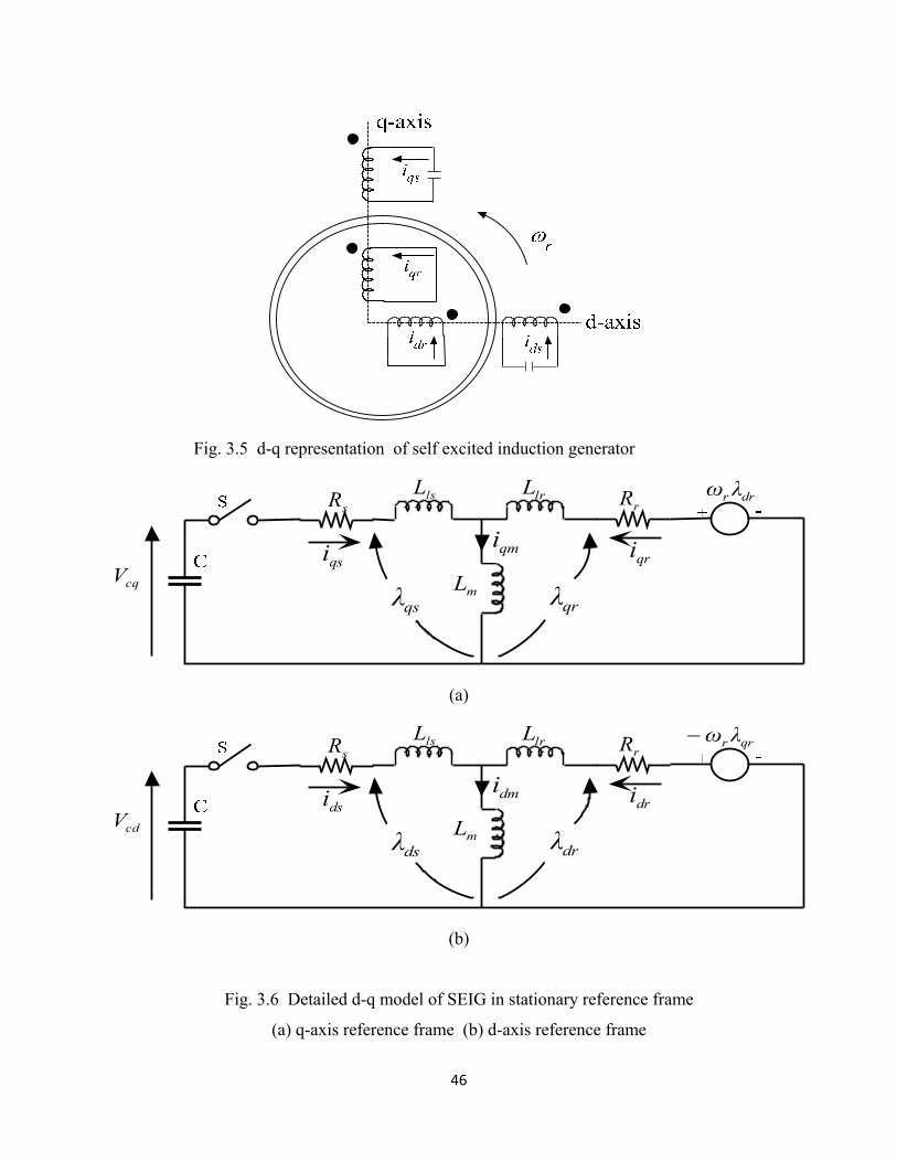
46

Fig. 3.5 d-q representation of self excited induction generator

(a)

(b)

Fig. 3.6 Detailed d-q model of SEIG in stationary reference frame

(a) q-axis reference frame (b) d-axis reference frame

cqV

sR lsL lrLrR

mL

qmiqsi qri

drr λω

qsλ qrλ

cdV

sR lsL lrLrR

mL

dmidsi dri

qrr λω

dsλ drλ

47

and the rotational voltage in the d axis of the rotor circuit is

qrr λω rω qrrqsm iLiL 0qrr λω

qrr λω rω qrrqsm iLiL drK (3.12)

where 0qrrdrK and 0drrqrK are constants, which represent the initial induced voltages

along the d-axis and q-axis, respectively. The constants drK and qrK are due to the remnant or

residual magnetic flux in the core, and r is the equivalent electrical rotor speed in radians/second.

That is,

Electrical speed number of pole pairs mechanical speed

The matrix equation for the d-q model of a self-excited induction generator, in the stationary

stator reference frame, using the SEIG model given in Fig. 3.6 and from equations (3.11) and

(3.12), is given as:

0

0

0

0

rrrrmmr

rrrrmrm

mss

mss

pLRLωpLLω

LωpLRLωpL

pLpCpLR

pLpCpLR

010

001

dr

qr

ds

qs

i

i

i

i

dr

qr

cd

cq

K

K

V

V

0

0

(3.13)

Z IV VV

Where Z is the impedance matrix, IVis the stator and rotor currents vector and VVis the voltage

vector due to initial conditions.

3.4 Conditions for Self Excitation in Induction Generator

Basically an induction machine is modeled using RLC circuit parameters. Self excitation in

an induction generator is the growth of current and the associated increase in the voltage across the

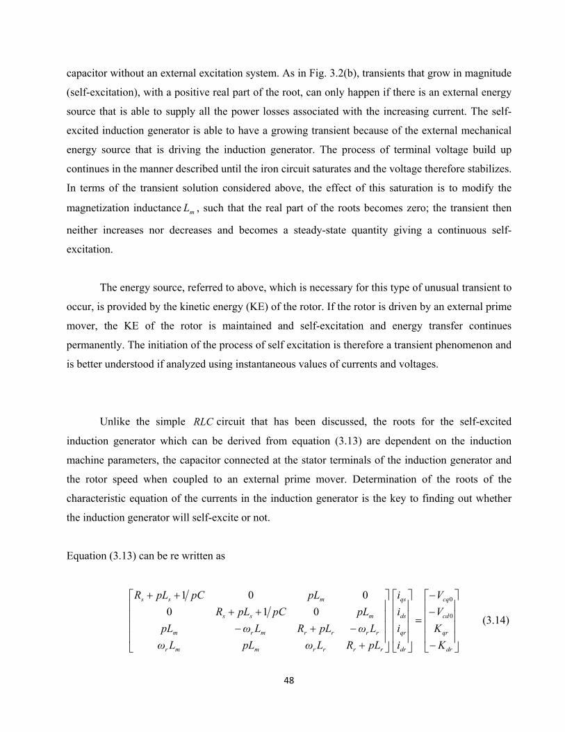
48

capacitor without an external excitation system. As in Fig. 3.2(b), transients that grow in magnitude

(self-excitation), with a positive real part of the root, can only happen if there is an external energy

source that is able to supply all the power losses associated with the increasing current. The self-

excited induction generator is able to have a growing transient because of the external mechanical

energy source that is driving the induction generator. The process of terminal voltage build up

continues in the manner described until the iron circuit saturates and the voltage therefore stabilizes.

In terms of the transient solution considered above, the effect of this saturation is to modify the

magnetization inductance mL , such that the real part of the roots becomes zero; the transient then

neither increases nor decreases and becomes a steady-state quantity giving a continuous self-

excitation.

The energy source, referred to above, which is necessary for this type of unusual transient to

occur, is provided by the kinetic energy (KE) of the rotor. If the rotor is driven by an external prime

mover, the KE of the rotor is maintained and self-excitation and energy transfer continues

permanently. The initiation of the process of self excitation is therefore a transient phenomenon and

is better understood if analyzed using instantaneous values of currents and voltages.

Unlike the simple RLC circuit that has been discussed, the roots for the self-excited

induction generator which can be derived from equation (3.13) are dependent on the induction

machine parameters, the capacitor connected at the stator terminals of the induction generator and

the rotor speed when coupled to an external prime mover. Determination of the roots of the

characteristic equation of the currents in the induction generator is the key to finding out whether

the induction generator will self-excite or not.

Equation (3.13) can be re written as

rrrrmmr

rrrrmrm

mss

mss

pLRLωpLLω

LωpLRLωpL

pLpCpLR

pLpCpLR

010

001

dr

qr

ds

qs

i

i

i

i

dr

qr

cd

cq

K

K

V

V

0

0

(3.14)

49

3.4.1 Direct matrix inversion

The equation (3.14) representing a self-excited induction generator can be solved by

applying Cramer’s rule or by finding the inverse of the impedance matrix, to determine the current

expression.

Cramer’s rule [1] is a mathematical tool for finding one of the variables in an unknown

vector in a matrix equation based on the calculation of determinants. Applying Cramer’s rule to

equation (3.14) results in

dsi

rrrrmmr

rrrrmrm

mss

mss

rrrrdrmr

rrrrqrm

mcd

mcqss

pLRLωpLLω

LωpLRLωpL

pLpCpLR

pLpCpLR

pLRLωKLω

LωpLRKpL

pLV

pLVpCpLR

010

001

00

01

0

0

(3.15)

Since the characteristic equation of the d-axis stator current is the determinant of the

denominator, only the denominator part of dsi will be expanded. The determinant of the numerator

will be represented by a variable U , which is dependent on the machine parameters, initial

conditions, capacitance and electrical rotor speed. U affects only the magnitude of the current dsi

and does not contain any information on the behavior of the resulting current. The determinants in

equation (3.15) can be evaluated [30] to give

dsi )/()( 22

012

23

34

45

56

6 pCApApApApApApA

U

(3.16)

where

6A 2C 4222 2 mmrsrs LLLLLL

50

5A 22C 2222mrsrsrmsrrss LRLRLLLRLLLR

4A 2C 22422222222 224)( mrsrmrmsrsrsrsrrrrs LRRωLωLLLLRRLRLRLωL

C2 22mrrs LLLL

3A 2 222222222 2 mrrsrrsrsssrrrsmrrsrs LRRLLLRCRLRRRLωRLLωRLLC

2A CLs2 )( 222rrr RLω 22CRs )( 222

rrr RLω 222 rmr ωCLL 2rL rsr CRRL4

1A CRs2 )( 222rrr RLω rr LR2

0A )( 222rrr RLω (3.17)

Analyzing the denominator of equation (3.16) is sufficient to determine whether initiation of

self-excitation will occur. To determine if there is an onset of self excitation, or not, the

denominator of equation (3.16) is set to zero. That is

012

23

34

45

56

6 ApApApApApApA 0 (3.18)

Equation (3.18) is a sixth order characteristic equation and it has six distinct roots which are first

order complex roots in the form of

)( 11 ωjσp )( 11 ωjσp )( 22 ωjσp )( 22 ωjσp )( 33 ωjσp )( 33 ωjσp 0

(3.19)

If any of the roots has a positive real part, then at that given specific operating point there will be

self-excitation.

The current and voltage will grow until the magnetizing inductance saturates and makes the

real part of the roots zero, which shows that there is a continuous oscillation (Alternating Current

and Voltage) as long as the prime mover is driving the induction generator. The transient and steady

state solution due to each of the roots can be obtained by using partial fraction expansion.

51

3.5 Minimum Speed and Capacitance for Self Excitation

The induction machine used as the SEIG in this investigation is a three-phase squirrel cage

induction machine with specification: 4 pole, 415V delta connected, 14.6A, 10hp, 50Hz. The d-q

model, shown in Fig. 3.6 is used because it provides the complete solution, transient and steady

state, of the self-excitation process.

When the three capacitors are connected in star the voltage rating of each capacitor is equal

to the rated phase voltage. However, if the capacitors are connected in delta the voltage rating of

each capacitor should be equal to the line-to-line voltage. In delta connected capacitors, even

though the voltage rating of each capacitor is higher than the rating of the capacitors in star

connection by a factor of 3 , the magnitude of the capacitance is lower by a factor 3, i.e. 1/3 of the

capacitance in the star connection.

When in the induction machine equivalent circuit, as shown in Fig. 3.6, with the switch S

closed, and the machine is driven by a prime mover, voltage will start to develop at a corresponding

minimum speed. The minimum speed for the onset of self-excitation can be obtained by solving the

roots of the 6th order polynomial equation given in equation (3.18) with different resistive loads

and then searching if there is a positive real part in the roots. The minimum capacitance required for

a given rotor speed of the induction generator can be found by fixing the rotor speed and then

increasing the value of the capacitance until one of the real parts of the roots changes from negative

to positive, passing through zero. The value of capacitance that makes the real part of one of the

complex roots greater than zero is the minimum value of capacitance required for self excitation. To

have a smooth plot of the minimum rotor speed versus minimum capacitance requirement, the

capacitance was incremented by a small value. The detail of this procedure, theoretical

determination of the minimum speed and minimum capacitance for a fixed speed by incrementing

the capacitance, is given in the flow chart of Fig. 3.7. The simulated result is shown in Fig.3.8.

Another way of finding the minimum rotor speed and corresponding minimum capacitance

required for self-excitation is first to set the capacitance at a given value and then increase the rotor

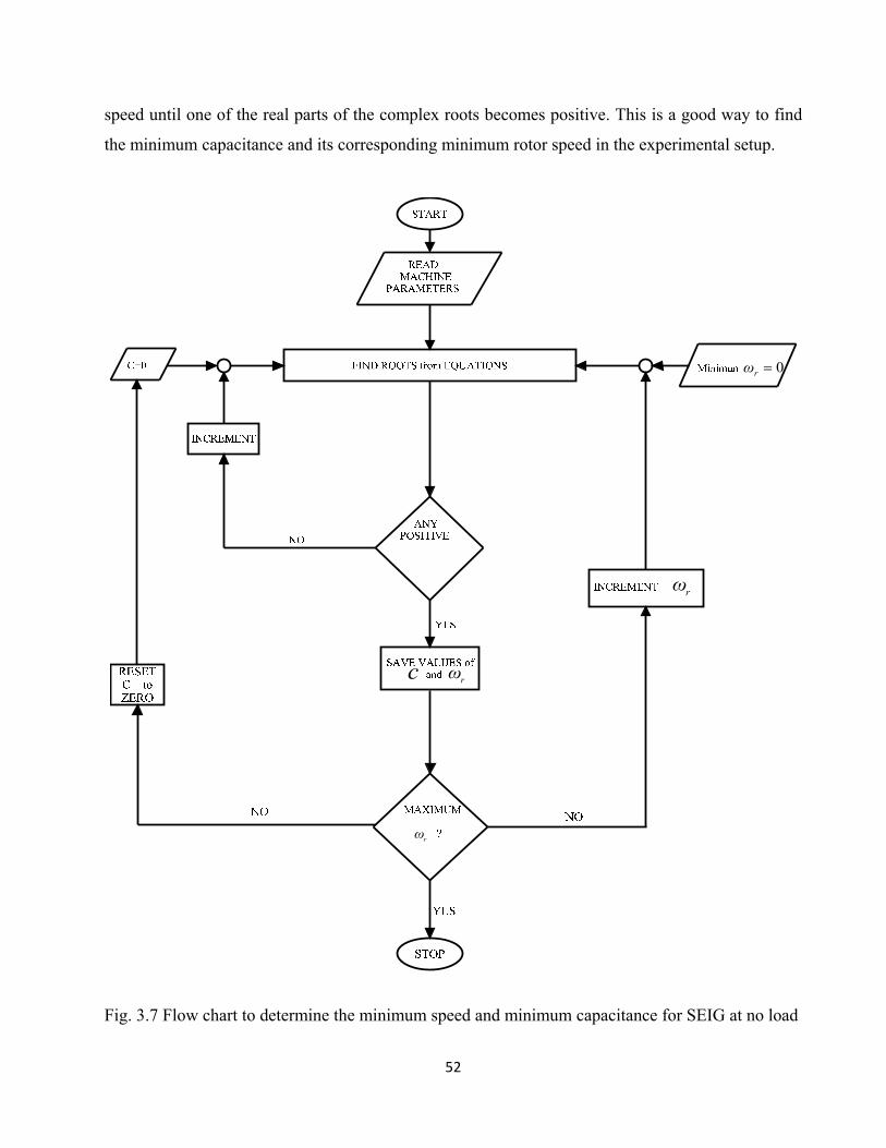
52

speed until one of the real parts of the complex roots becomes positive. This is a good way to find

the minimum capacitance and its corresponding minimum rotor speed in the experimental setup.

Fig. 3.7 Flow chart to determine the minimum speed and minimum capacitance for SEIG at no load

rωc

rω

rω

0rω

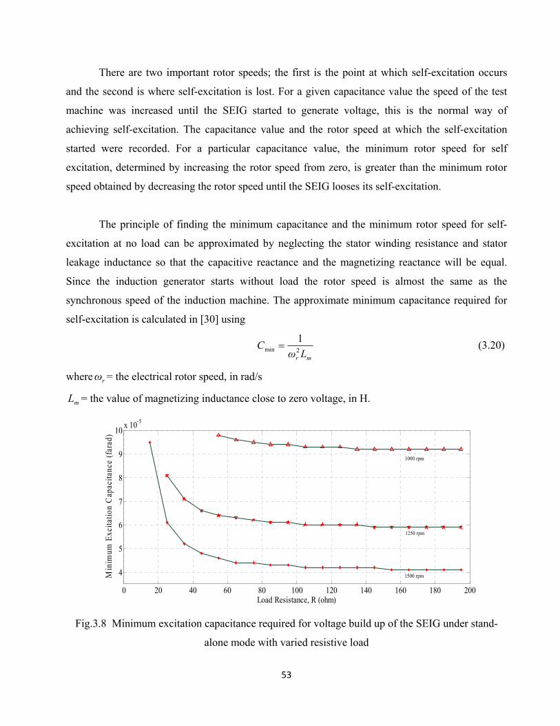
53

There are two important rotor speeds; the first is the point at which self-excitation occurs

and the second is where self-excitation is lost. For a given capacitance value the speed of the test

machine was increased until the SEIG started to generate voltage, this is the normal way of

achieving self-excitation. The capacitance value and the rotor speed at which the self-excitation

started were recorded. For a particular capacitance value, the minimum rotor speed for self

excitation, determined by increasing the rotor speed from zero, is greater than the minimum rotor

speed obtained by decreasing the rotor speed until the SEIG looses its self-excitation.

The principle of finding the minimum capacitance and the minimum rotor speed for self-

excitation at no load can be approximated by neglecting the stator winding resistance and stator

leakage inductance so that the capacitive reactance and the magnetizing reactance will be equal.

Since the induction generator starts without load the rotor speed is almost the same as the

synchronous speed of the induction machine. The approximate minimum capacitance required for

self-excitation is calculated in [30] using

mr LωC

2min

1 (3.20)

where rω = the electrical rotor speed, in rad/s

mL = the value of magnetizing inductance close to zero voltage, in H.

Fig.3.8 Minimum excitation capacitance required for voltage build up of the SEIG under stand-

alone mode with varied resistive load

0 20 40 60 80 100 120 140 160 180 200

4

5

6

7

8

9

10x 10-5

Load Resistance, R (ohm)

Min

imum

Exc

itatio

n C

apac

itanc

e (f

arad

)

1250 rpm

1500 rpm

1000 rpm

54

In no load motoring or generating operation the synchronous speed is almost equal to the

electrical rotor speed. The SEIG needs to be started at no load. Hence it can be generalized that the

capacitance required for the onset of self-excitation in the SEIG rotating at a rotor speed of r , is

almost equal to the capacitance required to have a unity power factor in a motoring application, as

the induction motor operates at no load and with an angular supply frequency of r .

3.6 Simulation of self-excited induction generator with R-L Load

In conducting an experimental analysis of a self-excited induction generator, it is difficult to

get continuous values of a capacitance and determine the corresponding speed. Mostly the

components are in discreet values. It is also hard to see the condition of the self-excitation beyond

the rated values of the machine as it can damage the machine. Simulation is extremely useful in

predicting the condition of self-excitation within the rated values of the machine and/or beyond

these rated values.

3.6.1 The modeling of self-excitation process

To find the dynamics of a self-excited induction generator a mathematical model is

developed. The solution of this mathematical model gives the complete characteristics comprising

of transient and steady state for the voltage, current, power and frequency of a self-excited

induction generator. With the help of this mathematical model the dynamic values of voltage,

current and power of the SEIG at any given time can be evaluated. The mathematical model takes

into account the initial conditions in the induction generator, namely the initial voltage in the

exciting capacitors and the initial induced voltage due to remnant magnetic flux in the magnetic

core.

3.6.2 The dynamic representation of SEIG with RL load

The SEIG equivalent circuit shown in Fig. 3.6 can be loaded with a resistive load by

connecting a resistance RL across the capacitor, C. With resistive load equation (3.13) is modified

to the following equation

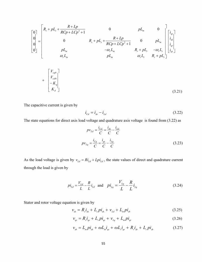
55

0

0

0

0

2

2

0 01

0 01

s s m

s s m

m r m r r r r

r m m r r r r

R LpR pL pL

RCp LCp

R LpR pL pL

RCp LCp

pL L R pL L

L pL L R pL

dr

qr

ds

qs

i

i

i

i

d

q

cd

cq

K

K

V

V

0

0

(3.21)

The capacitive current is given by

LddsCd iii (3.22)

The state equations for direct axis load voltage and quadrature axis voltage is found from (3.22) as

C

i

C

i

C

ipv LddsCd

Ld

C

i

C

i

C

ipv LqqsCq

Lq (3.23)

As the load voltage is given by Ld Ld Ldv Ri Lpi , the state values of direct and quadrature current

through the load is given by

LdLd Ld

V Rpi i

L L

and Lq

Lq

Lq iL

R

L

Vpi (3.24)

Stator and rotor voltage equation is given by

dsv dssiR dss piL Ldv drm piL (3.25)

qsv qssiR qss piL Lqv qrm piL (3.26)

drv dsm piL qsmiLω qrriLω drriR drr piL (3.27)

56

qrv dsmiLω qsm piL qrriR qrr piL drriLω (3.28)

Isolating the differential terms of the direct and quadrature currents of the rotor

mdr L

pi1

)( Lddssdssds vpiLiRv (3.29)

mqr L

pi1

)( Lqqssqssqs vpiLiRv (3.30)

Isolating qspi ,

2m

qsm s r

Lpi

L L L

( )qr m ds r qr r drv L i R i L i

2r

m s r

L

L L L

( )qs r qs Lqv R i v

(3.31)

Assuming the following leakage coefficient:

2

1

m s r

KL L L

qs mpi L K ( )qr m ds r qr r drv L i R i L i rL K ( )qs r qs Lqv R i v (3.32)

ds mpi L K ( )dr m qs r dr r qrv L i R i L i rL K ( )ds r ds Ldv R i v (3.33)

(1 )( )s r

qr qs s qs Lqm

KL Lpi v R i v

L

sL K ( )qr m ds r qr r drv L i R i L i

(3.34)

As m

rsm L

KLLKL

)1( , so

( )qr m qs s qs Lqpi L K v R i v sL K ( )qr m ds r qr r drv L i R i L i

(3.35)

And for direct axis

( )dr m ds s ds Ldpi L K v R i v sL K ( )dr m qs r dr r qrv L i R i L i (3.36)

The state space matrix involving an RL load is given by

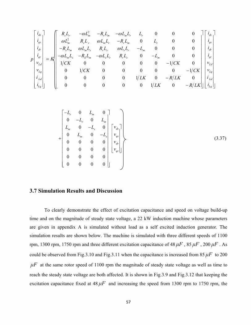
57

ds

qs

dr

qr

Ld

Lq

Ld

Lq

i

i

i

ip

v

v

i

i

K

2

2

0 0 0

0 0 0

0 0 0

0 0 0

1 0 0 0 0 0 1 0

0 1 0 0 0 0 0 1

0 0 0 0 1 0 0

0 0 0 0 0 1 0

s r m r m m r r

m s r m r r m r

s m m s r s s r m

m s S m s r r s m

R L L R L L L L

L R L L L R L L

R L L L R L L L L

L L R L L L R L L

CK CK

CK CK

LK R LK

LK R LK

ds

qs

dr

qr

Ld

Lq

Ld

Lq

i

i

i

i

v

v

i

i

0 0

0 0

0 0

0 0

0 0 0 0

0 0 0 0

0 0 0 0

0 0 0 0

r m

r m

m s

m s

L L

L L

L L

L L

ds

qs

dr

qr

v

v

v

v

(3.37)

3.7 Simulation Results and Discussion

To clearly demonstrate the effect of excitation capacitance and speed on voltage build-up

time and on the magnitude of steady state voltage, a 22 kW induction machine whose parameters

are given in appendix A is simulated without load as a self excited induction generator. The

simulation results are shown below. The machine is simulated with three different speeds of 1100

rpm, 1300 rpm, 1750 rpm and three different excitation capacitance of 48 Fμ , 85 Fμ , 200 Fμ . As

could be observed from Fig.3.10 and Fig.3.11 when the capacitance is increased from 85 Fμ to 200

Fμ at the same rotor speed of 1100 rpm the magnitude of steady state voltage as well as time to

reach the steady state voltage are both affected. It is shown in Fig.3.9 and Fig.3.12 that keeping the

excitation capacitance fixed at 48 Fμ and increasing the speed from 1300 rpm to 1750 rpm, the

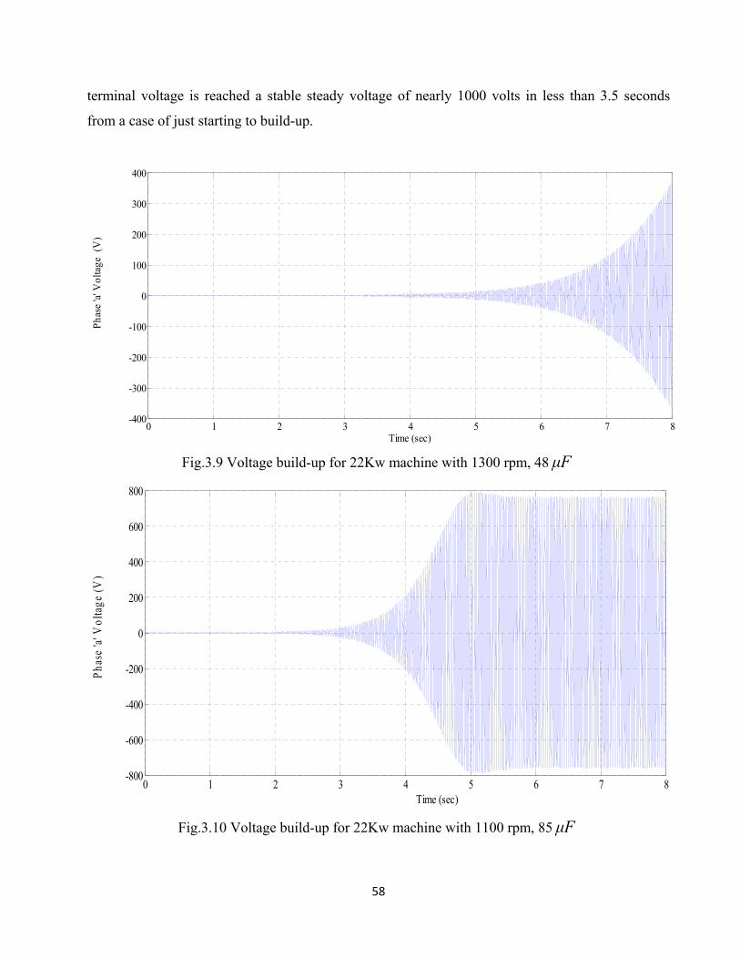
58

terminal voltage is reached a stable steady voltage of nearly 1000 volts in less than 3.5 seconds

from a case of just starting to build-up.

Fig.3.9 Voltage build-up for 22Kw machine with 1300 rpm, 48 Fμ

Fig.3.10 Voltage build-up for 22Kw machine with 1100 rpm, 85 Fμ

0 1 2 3 4 5 6 7 8-400

-300

-200

-100

0

100

200

300

400

Time (sec)

Pha

se 'a

' Vol

tage

(V

)

0 1 2 3 4 5 6 7 8-800

-600

-400

-200

0

200

400

600

800

Time (sec)

Pha

se 'a

' Vol

tage

(V

)

59

Fig.3.11 Voltage build-up for 22Kw machine with 1100 rpm, 200 Fμ

Fig.3.12 Voltage build-up for 22Kw machine with 1750 rpm, 48 Fμ

0 1 2 3 4 5 6 7 8-1000

-800

-600

-400

-200

0

200

400

600

800

1000

Time (sec)

Pha

se 'a

' Vol

tage

(V

)

0 1 2 3 4 5 6 7 8-1500

-1000

-500

0

500

1000

1500

Time (sec)

Pha

se 'a

' Vol

tage

(V

)

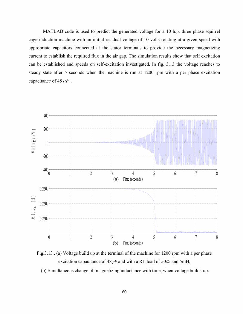
60

MATLAB code is used to predict the generated voltage for a 10 h.p. three phase squirrel

cage induction machine with an initial residual voltage of 10 volts rotating at a given speed with

appropriate capacitors connected at the stator terminals to provide the necessary magnetizing

current to establish the required flux in the air gap. The simulation results show that self excitation

can be established and speeds on self-excitation investigated. In fig. 3.13 the voltage reaches to

steady state after 5 seconds when the machine is run at 1200 rpm with a per phase excitation

capacitance of 48 Fμ .

Fig.3.13 . (a) Voltage build up at the terminal of the machine for 1200 rpm with a per phase

excitation capacitance of 48 Fμ and with a RL load of 50 and 5mH,

(b) Simultaneous change of magnetizing inductance with time, when voltage builds-up.

0 1 2 3 4 5 6 7 8-400

-200

0

200

400

Time (seconds)

Vol

tage

(V

)

0 1 2 3 4 5 6 7 8

0.2609

0.2609

0.2609

Time (seconds)

MI,

Lm

(H

)

(a)

(b)

61

Fig.3.14 shows the voltage build up for 1400 rpm with same excitation capacitance and load.

Fig.3.14 (a) Voltage build up at 1400 rpm and 48 Fμ for RL load of 50 and 5mH, (b)

Simultaneous change of magnetizing inductance with time, when voltage builds-up.

Fig.3.15 shows the voltage build up for 1800 rpm with same excitation capacitance and load.

Fig.3.15 (a) Voltage build up at 1800 rpm and 48 Fμ for RL load of 50 and 5mH, (b)

Simultaneous change of magnetizing inductance with time, when voltage builds-up.

0 1 2 3 4 5 6 7 8-400

-200

0

200

400

Time (seconds)

Vol

tage

(V

)

0 1 2 3 4 5 6 7 8

0.2609

0.2609

0.2609

Time (seconds)

MI,

Lm

(H

)

0 1 2 3 4 5 6 7 8-400

-200

0

200

400

Time (seconds)

Vol

tage

(V

)

0 1 2 3 4 5 6 7 80.2609

0.2609

0.2609

0.2609

0.2609

Time (seconds)

MI,

Lm

(H

)

(a)

(b)

(a)

(b)

62

Fig.3.16 (a)Voltage build up at 1800 rpm and 100 Fμ for RL load of 50 and 5mH, (b)

Simultaneous change of magnetizing inductance with time, when voltage builds-up.

In Fig.3.16 the voltage builds up is shown when the machine is run at 1800 rpm with the

same load but with an excitation capacitance of 100 Fμ . Fig.3.17, Fig.3.18 and Fig.3.19 show the

generated voltage, line current, load current, active power, reactive power and electromagnetic

torque responses. The load is 50Ω and 5mH. Fig.3.17 is for a speed of 1400rpm with excitation

capacitance of 48µF. Fig.3.18 is for a speed of 1800 rpm with 48µF excitation capacitance. Fig.3.19

is for an excitation capacitance of 100µF, at 1800 rpm speed.

0 1 2 3 4 5 6 7 8-400

-200

0

200

400

Time (seconds)

Vol

tage

(V

)

0 1 2 3 4 5 6 7 80.2609

0.2609

0.2609

0.2609

0.2609

Time (seconds)

MI,

Lm

(H

)

(a)

(b)

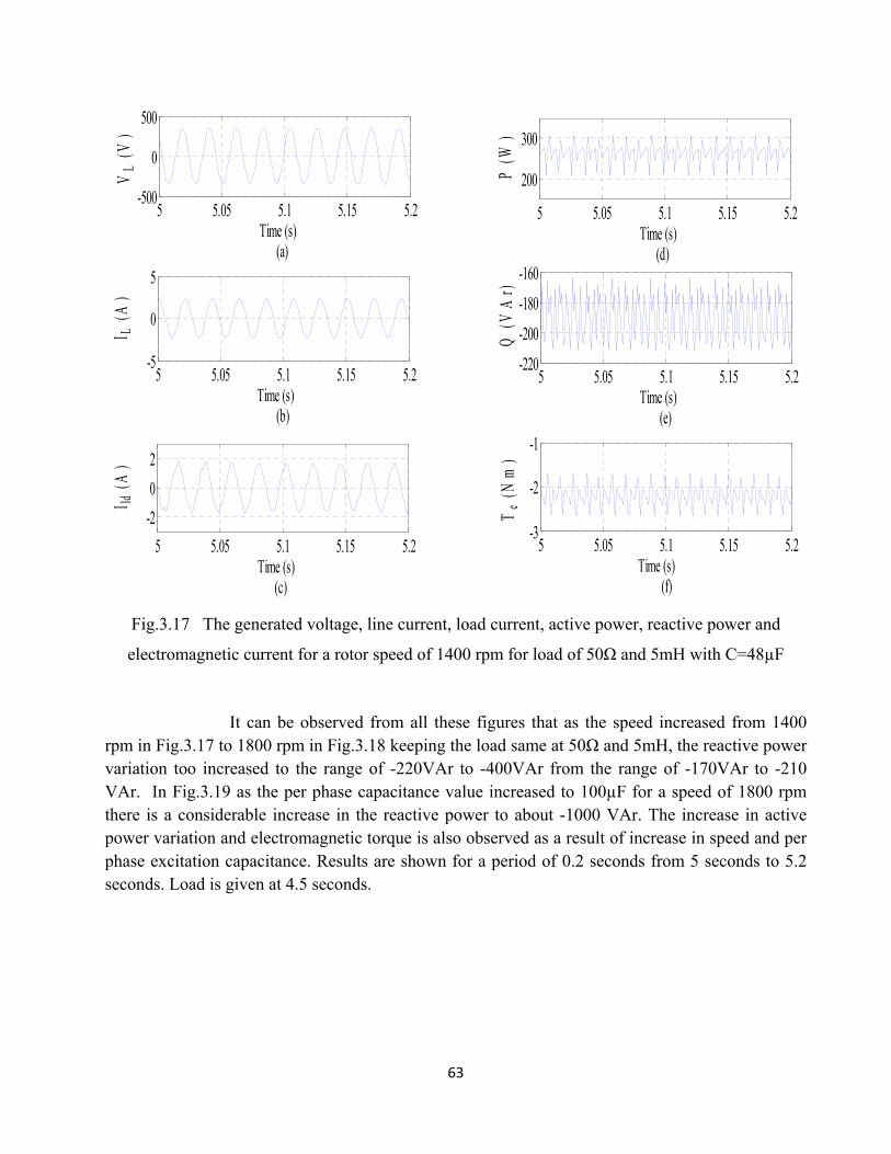
63

Fig.3.17 The generated voltage, line current, load current, active power, reactive power and

electromagnetic current for a rotor speed of 1400 rpm for load of 50Ω and 5mH with C=48µF

It can be observed from all these figures that as the speed increased from 1400 rpm in Fig.3.17 to 1800 rpm in Fig.3.18 keeping the load same at 50Ω and 5mH, the reactive power variation too increased to the range of -220VAr to -400VAr from the range of -170VAr to -210 VAr. In Fig.3.19 as the per phase capacitance value increased to 100µF for a speed of 1800 rpm there is a considerable increase in the reactive power to about -1000 VAr. The increase in active power variation and electromagnetic torque is also observed as a result of increase in speed and per phase excitation capacitance. Results are shown for a period of 0.2 seconds from 5 seconds to 5.2 seconds. Load is given at 4.5 seconds.

5 5.05 5.1 5.15 5.2-500

0

500

Time (s) (a)

VL

(V

)

5 5.05 5.1 5.15 5.2

200

300

Time (s) (d)

P (

W)

5 5.05 5.1 5.15 5.2

-2

0

2

Time (s) (c)

I ld (

A)

5 5.05 5.1 5.15 5.2-220

-200

-180

-160

Time (s) (e)

Q (

VA

r)

5 5.05 5.1 5.15 5.2-5

0

5

Time (s) (b)

I L (

A)

5 5.05 5.1 5.15 5.2-3

-2

-1

Time (s) (f)

Te

(Nm

)

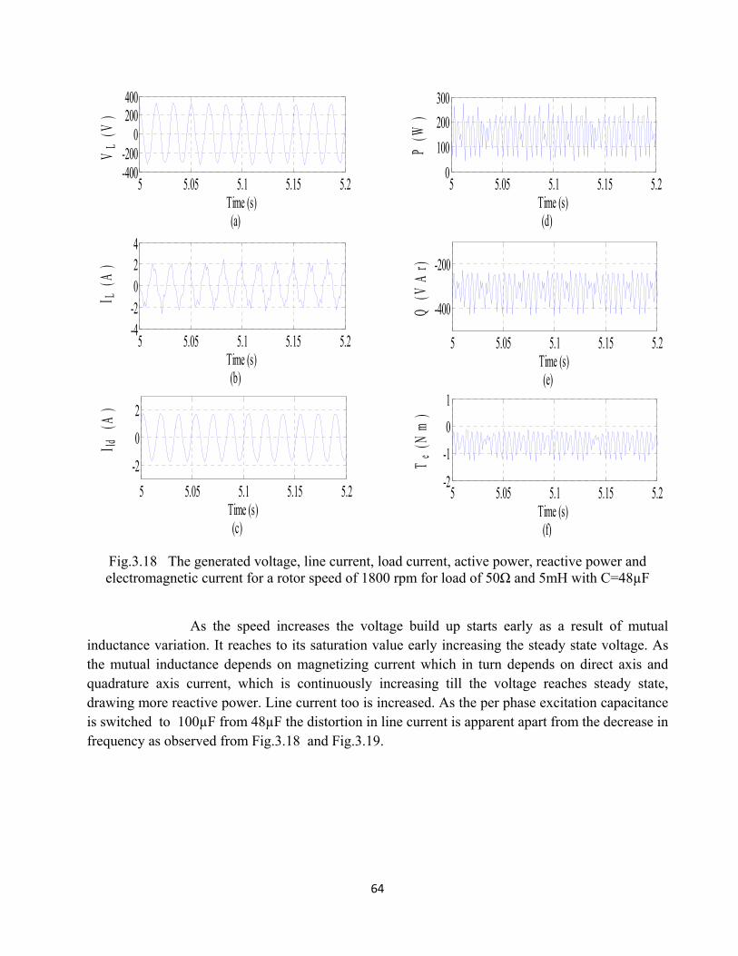
64

Fig.3.18 The generated voltage, line current, load current, active power, reactive power and electromagnetic current for a rotor speed of 1800 rpm for load of 50Ω and 5mH with C=48µF

As the speed increases the voltage build up starts early as a result of mutual inductance variation. It reaches to its saturation value early increasing the steady state voltage. As the mutual inductance depends on magnetizing current which in turn depends on direct axis and quadrature axis current, which is continuously increasing till the voltage reaches steady state, drawing more reactive power. Line current too is increased. As the per phase excitation capacitance is switched to 100µF from 48µF the distortion in line current is apparent apart from the decrease in frequency as observed from Fig.3.18 and Fig.3.19.

5 5.05 5.1 5.15 5.2-400-200

0200400

Time (s)(a)

VL

(V

)

5 5.05 5.1 5.15 5.20

100

200

300

Time (s)(d)

P (

W)

5 5.05 5.1 5.15 5.2-4-2024

Time (s)(b)

I L (

A)

5 5.05 5.1 5.15 5.2

-400

-200

Time (s)(e)

Q (

VA

r)

5 5.05 5.1 5.15 5.2

-2

0

2

Time (s)(c)

I ld (

A)

5 5.05 5.1 5.15 5.2-2

-1

0

1

Time (s)(f)

Te

(Nm

)

65

Fig.3.19 The generated voltage, line current, load current, active power, reactive power and electromagnetic current for a rotor speed of 1800 rpm for load of 50Ω and 5mH with C=100µF

3.8 Conclusion

It is shown that, a series R-L-C circuit with initial capacitor voltage can have sustained

oscillations if the real part of the characteristic roots is zero that means the resistance in the circuit

is zero. It is shown in section 3.2 that the self excitation occurs in an induction generator when the

capacitive reactance is close to but slightly less than the magnetizing reactance. It is also shown that

with constant speed and excitation capacitance, as the load on SEIG increases, speed decreases, So

generated voltage and frequency decrease. D-Q axis model of SEIG with excitation capacitance is

derived. Condition for self excitation in SEIG, with reference to characteristic roots of the system is

derived. Requirements of minimum capacitance and speed for self excitation are derived. A flow

5 5.05 5.1 5.15 5.2-400-200

0200400

Time (s)(a)

VL

(V

)

5 5.05 5.1 5.15 5.2-1000

0

1000

Time (s)(d)

P (

W)

5 5.05 5.1 5.15 5.2

-5

0

5

Time (s)(b)

I L (

A)

5 5.05 5.1 5.15 5.2-2000

-1000

0

Time (s)(e)

Q (

VA

r)

5 5.05 5.1 5.15 5.2-2

0

2

Time (s)(c)

I ld (

A)

5 5.05 5.1 5.15 5.2-15-10-505

Time (s)(f)

Te

(Nm

)

66

chart for computer program on finding minimum speed and minimum capacitance is discussed.

Graph for minimum excitation capacitance required for voltage build-up of SEIG, as a function of

load resistance is also plotted. Dynamic D-Q axis model of SEIG with R-L load is derived. Finally

simulation results on voltage build-up transients are presented and discussed. The waveforms of

phase voltage, mutual inductance, line current, load current, real power, reactive power and

electromagnetic torque under different conditions of excitation capacitance and speed are plotted

and discussed. In the next chapter, closed loop control of SEIG with PWM VSI is presented.

67

CHAPTER 4

CLOSED LOOP CONTROL OF SEIG USING

PWM-VSI

4.1 Introduction

The main drawback of using induction generators excited by three AC capacitors is their

inherently poor voltage regulation and uncontrollable frequency of operation. The output voltage of

a SEIG can be controlled by introducing an appropriate voltage regulating scheme. A number of

schemes have been suggested for this purpose. However, the variation of the frequency of the SEIG

with load and speed cannot be regulated by static means. As a result the equipment supplied by the

three-phase SEIG discussed in Chapter 3 should be frequency insensitive (e.g. heater, water pump,

lighting, battery charging etc).

The scheme based on switched capacitors finds limited application because it regulates the

terminal voltage in discrete steps. A saturable reactor scheme of voltage regulation involves a

potentially large size and weight, due to the necessity of a large saturating inductor. In the

short/long shunt configuration the series capacitor used causes the problem of resonance while

supplying power to an inductive load.

In a three phase capacitor bank excited induction generator, the value of capacitance should be

varied so that the terminal voltage remains constant at different rotor speeds. It is also shown that

the value of capacitance is influenced by the load as well as by the load power factor. The problem

is further aggravated by the uncertainty of the machine to re-excite after a short circuit unless some

charge is provided. Loss of self-excitation could be disastrous in applications like aircraft power

supplies. There should be a way to avoid this problem. An isolated induction generator with an

excitation system provided by a single capacitor on the DC link side of the inverter can re-excite

68

even after a short circuit. Since a battery is required to control the switching of the IGBTs of the

inverter, the same battery can be used for the initiation of voltage build up using scalar or vector

control.

4.2 Closed loop Voltage Control of SEIG

In conventional self-excited variable-speed induction generators with a bank of capacitors

connected across the machine terminals, the value of capacitance required is almost inversely

proportional to the square of the prime mover speed, requiring large values of capacitance at low

speeds. Uncontrolled variable voltage and frequency output of a self-excited induction generator is

its major drawback which can be overcome by a large extent by using a power converter with a

large DC-side capacitor connected between the induction generator and the power network.

When the excitation comes from the DC link capacitor of the converter, as covered in this

chapter, then varying the current flowing to the generator by controlling the switching of the IGBTs

varies the flux in the generator. Due to the switching of the inverter/rectifier the single DC side

capacitor acts like a three-phase capacitor. The reactive current or the VAR required by the

induction generator comes from the PWM converter through adjustment of magnitude and phase

angle of reference sine waves. The dc link capacitor meets the excitation energy required by SEIG.

In a grid connected induction generator, the grid acts as a stiff voltage source so that the

generator control structure is similar to a standard drive with sinusoidal front-end converter, i.e. by

varying the modulation index, the terminal voltage at the induction generator can be varied with the

rotor speed while the DC bus is maintained at constant voltage.

For an induction generator operating in stand-alone mode there should be a system that

regulates the output voltage. The output voltage is the DC voltage and the control system, which is

implemented using scalar control, is required to keep this DC voltage at a constant level. The

frequency of the generator voltage can vary with speed but the aim is to have constant peak voltage

and as a result to have constant DC voltage. Once a constant DC voltage is achieved, a DC load can

69

use it directly. If required an inverter can be used to produce a constant voltage and frequency AC

output. The electrical and mechanical connections for an isolated induction generator driven by a

wind turbine are shown in Fig. 4.1. To simplify the diagram the control system is not included in

Fig. 4.1.

In Fig. 4.1 the turbine rotor speed will be varied depending on the wind speed. The system is

loaded by a DC load connected at the terminals of the DC capacitor or an AC load can be connected

via a second inverter that adjusts the frequency and peak voltage of the generated AC power supply.

Induction generator is excited from a single DC capacitor by using an inverter arrangement. The

voltage build up process is started from a small voltage in a charged DC capacitor or from a battery.

During the voltage build up process the DC capacitor gets its charge from the induction generator

via the rectifier.

Scalar control of induction machine means control of the magnitude of voltage and

frequency so as to achieve suitable torque and speed. Scalar control disregards the coupling effect

on the generator. The voltage will be set to control the flux and the frequency in order to control the

torque. Flux and torque are functions of frequency and voltage. Scalar control is different from

vector control in which both magnitude and phase alignment of the vector variables are controlled.

The main constraint on the use of a scalar control method for induction motors and generators is

related to the transient response. If shaft torque and speed are bandwidth-limited and torque varies

slowly, required speed response time varies from hundreds of milliseconds up to the order of almost

a second, scalar control may work appropriately. Hydropower and wind power applications have

slower mechanical dynamics. Therefore, the scalar control is still a good approach for renewable

energy applications. The fundamental objective behind the scalar method is to provide a controlled

slip operation.

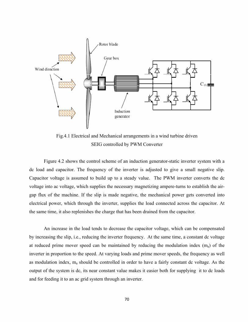
70

Fig.4.1 Electrical and Mechanical arrangements in a wind turbine driven

SEIG controlled by PWM Converter

Figure 4.2 shows the control scheme of an induction generator-static inverter system with a

dc load and capacitor. The frequency of the inverter is adjusted to give a small negative slip.

Capacitor voltage is assumed to build up to a steady value. The PWM inverter converts the dc

voltage into ac voltage, which supplies the necessary magnetizing ampere-turns to establish the air-

gap flux of the machine. If the slip is made negative, the mechanical power gets converted into

electrical power, which through the inverter, supplies the load connected across the capacitor. At

the same time, it also replenishes the charge that has been drained from the capacitor.

An increase in the load tends to decrease the capacitor voltage, which can be compensated

by increasing the slip, i.e., reducing the inverter frequency. At the same time, a constant dc voltage

at reduced prime mover speed can be maintained by reducing the modulation index (ma) of the

inverter in proportion to the speed. At varying loads and prime mover speeds, the frequency as well

as modulation index, ma should be controlled in order to have a fairly constant dc voltage. As the

output of the system is dc, its near constant value makes it easier both for supplying it to dc loads

and for feeding it to an ac grid system through an inverter.

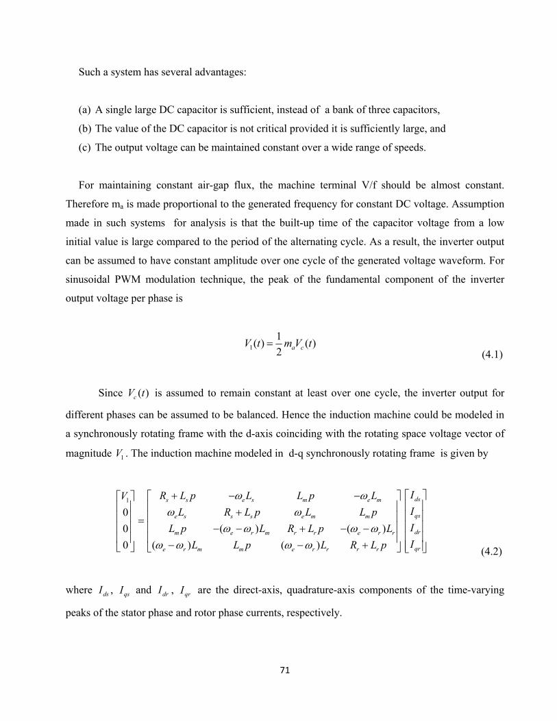
71

Such a system has several advantages:

(a) A single large DC capacitor is sufficient, instead of a bank of three capacitors,

(b) The value of the DC capacitor is not critical provided it is sufficiently large, and

(c) The output voltage can be maintained constant over a wide range of speeds.

For maintaining constant air-gap flux, the machine terminal V/f should be almost constant.

Therefore ma is made proportional to the generated frequency for constant DC voltage. Assumption

made in such systems for analysis is that the built-up time of the capacitor voltage from a low

initial value is large compared to the period of the alternating cycle. As a result, the inverter output

can be assumed to have constant amplitude over one cycle of the generated voltage waveform. For

sinusoidal PWM modulation technique, the peak of the fundamental component of the inverter

output voltage per phase is

1

1( ) ( )

2 a cV t m V t (4.1)

Since ( )cV t is assumed to remain constant at least over one cycle, the inverter output for

different phases can be assumed to be balanced. Hence the induction machine could be modeled in

a synchronously rotating frame with the d-axis coinciding with the rotating space voltage vector of

magnitude 1V . The induction machine modeled in d-q synchronously rotating frame is given by

1

0

0

0

V

( ) ( )

( ) ( )

s s e s m e m

e s s s e m m

m e r m r r e r r

e r m m e r r r r

R L p L L p L

L R L p L L p

L p L R L p L

L L p L R L p

ds

qs

dr

qr

I

I

I

I

(4.2)

where dsI , qsI and drI , qrI are the direct-axis, quadrature-axis components of the time-varying

peaks of the stator phase and rotor phase currents, respectively.

72

As the saturation of the main magnetic circuit is a critical factor, the magnetizing inductance

should be estimated at each stage of the computation from the magnetizing current, whose peak

value is given by

2 2( ) ( )m ds dr qs qrI I I I I

(4.3)

Because of the negative slip, the input current 1I to the machine has a negative real part

while the quadrature component lags behind the voltage. As a generator, the current output of the

machine is 1( )I , which leads the voltage by an angle, . The feedback diodes in the inverter

rectify the three-phase output currents. The rectified current, which is pulsating in nature with a

frequency of 6 sf , feeds the DC load connected across the capacitor. Depending on the value of C ,

the pulsating current causes a corresponding ripple in the voltage riding above the mean value. The

average voltage as well as the ripple go on increasing as long as the electrical power developed by

the generator exceeds the sum total of the power consumed by the load and the machine winding

copper losses.

4.3 System Description

The scheme which is implemented in this thesis is a scalar voltage and frequency control

scheme. The system description for the implementation of voltage control in an isolated induction

generator is shown in Fig.4.2. The implemented system starts its excitation process from an external

battery bV or it can be started from a charged capacitor. The external battery bV helps to charge the

capacitor and also to start the buildup of flux in the core. When the generated DC voltage rises to a

value higher than bV then the diode blocks the back flow of current to the battery. The diode can

also be replaced with a switch that is operated by comparing the value of the battery voltage and the

magnitude of the generated DC voltage in the capacitor.

As discussed in Chapter 3 a self-excited induction generator using three AC capacitors and

without any voltage control can start its voltage build up only from a remnant magnetic flux in the

73

core. The voltage build up starts when the induction generator is driven at a given speed and

appropriate capacitance is connected at its terminals. However, for a system with a single DC

capacitor, as explained in this Section, the voltage build up process cannot start from the remnant

flux in the core due to the following reasons:

a) There is no way of initiating the injection of exciting current into the induction generator via the

inverter using vector control.

b) The terminal voltage is not continuous because of the PWM switching in the inverter and the

current is not sinusoidal.

c) The power loss in the machine, the switching power losses in the inverter and the characteristic

of all the instantaneous losses due to PWM switching.

d) The losses in the generator increase because of the harmonics.

As a result an initial voltage is required in the DC capacitor to start the voltage build up

process. The initial voltage can be obtained from a previously charged DC capacitor or from a

battery connected to the DC capacitor. The easiest method is to utilize the battery that supplies

power to the IGBT drivers. The minimum initial voltage required in the DC capacitor is dependent

on the components used in the inverter/rectifier, their combined forward voltage drop in the

converter arrangement and the parameters of the induction generator. From the simulation, the

voltage build up process can start for voltage as low as 10V. However, to have a good control and

faster voltage build up process 48V is used. 48V is appropriate to implement the scheme at the

lowest speed and the 48V can also be obtained from connecting several standard commercially

available 12V batteries in series.

As discussed in Chapter 3 during the voltage build up process the magnetizing inductance, mL , in

an induction machine varies with the air gap voltage across it. The implementation of the variation

of magnetizing inductance in the model of induction generator depicts the actual variation in the

real system.

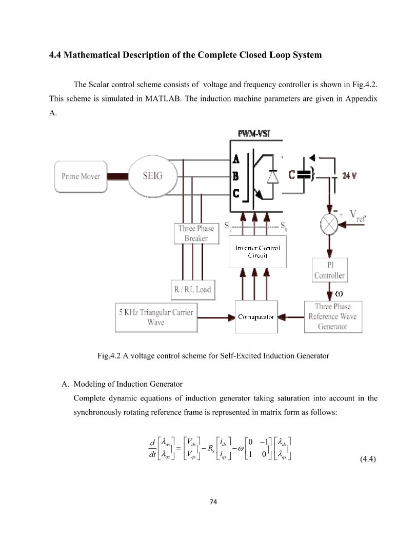
74

4.4 Mathematical Description of the Complete Closed Loop System

The Scalar control scheme consists of voltage and frequency controller is shown in Fig.4.2.

This scheme is simulated in MATLAB. The induction machine parameters are given in Appendix

A.

Fig.4.2 A voltage control scheme for Self-Excited Induction Generator

A. Modeling of Induction Generator

Complete dynamic equations of induction generator taking saturation into account in the

synchronously rotating reference frame is represented in matrix form as follows:

ds

qs

d

dt

0 1

1 0ds ds

sqs qs

V iR

V i

ds

qs

(4.4)

75

dr

qr

d

dt

0 1( )

1 0dr dr

r rqr qr

V iR

V i

dr

qr

(4.5)

B. Equations for electromagnetic torque and mechanical speed of the SEIG are expressed as

follows:

3

4e qr dr qr dr

PT i i

(4.6)

2

shaft e

r

P T Td

dt J

(4.7)

C. Modeling of 3- PWM-VSI

C.1 Model of the d.c side of the inverter

The capacitor voltage equation is governed by:

dcdc

IdV

dt C

(4.8)

where dcV is the voltage across the capacitor and dcI is the current flowing through

it.

The set point of dcV must be higher than the peak value of the generated phase

voltage so that the stator current can be controlled. Total DC link current dcI can be

expressed in terms of inverter switching function as

dc a ea b eb c ecI S i S i S i (4.9)

Where, the suffix e identifies compensator phase currents. The three switching

76

Functions ( cba SSS ,, ) take the value of 1 if the upper switch in the given inverter leg is

on and 0 if the lower switch is on and as

0 ecebea iii

bc

bceb

ab

abea z

vi

z

vi ,

C.2 Model of PWM Inverter

The phase voltages are given by

1

1

sin( )2 2dc dc

ao a nn

V VV SF A n t

(4.10)

1

1

sin( 120 )2 2dc dc

bo b nn

V VV SF A n t

(4.11)

1

1

sin( 240 )2 2dc dc

co c nn

V VV SF A n t

(4.12)

Line-to-line voltages generated by the inverter can be derived as:

ab ao boV V V (4.13)

bc bo coV V V (4.14)

ca co aoV V V (4.15)

D. Modeling of R-L Load

A R-L load connected to the stator terminals of induction generator can be represented in

the synchronously rotating reference frame as:

qs L Lqs L Lqs e L Lds

dV R i L i L i

dt

(4.16)

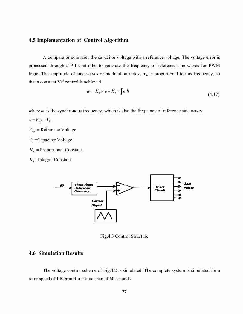
77

4.5 Implementation of Control Algorithm

A comparator compares the capacitor voltage with a reference voltage. The voltage error is

processed through a P-I controller to generate the frequency of reference sine waves for PWM

logic. The amplitude of sine waves or modulation index, ma is proportional to this frequency, so

that a constant V/f control is achieved.

P IK e K edt (4.17)

where is the synchronous frequency, which is also the frequency of reference sine waves

ref Ce V V

refV Reference Voltage

CV =Capacitor Voltage

PK Proportional Constant

IK =Integral Constant

Fig.4.3 Control Structure

4.6 Simulation Results

The voltage control scheme of Fig.4.2 is simulated. The complete system is simulated for a

rotor speed of 1400rpm for a time span of 60 seconds.

78

Fig.4.4 shows the voltage build-up over a span of 60 seconds reaching a steady state value

of 220V. Fig.4.5 shows the phase ‘a’ current of the self excited induction generator. DC link

capacitor voltage profile is shown in Fig.4.6. It reaches a voltage of 220V (set reference value)

within 4 seconds of starting the system. The error in voltage is tracked by a PI controller which in

turn regulates switching instants of the IGBTs. As the load is put to the system, the terminal voltage

reduced a little and as the load is removed, there is a increase in the terminal voltage as observed

from Fig.4.6. The three phase IGBT inverter controls the power flow to the SEIG thus maintaining

a constant voltage of 220V at the terminal of self-excited induction generator.

Fig.4.4 Terminal Voltage for a rotor speed of 1400rpm without load.

0 10 20 30 40 50 60-300

-200

-100

0

100

200

300

Time (sec)

Pha

se V

olta

ge (

V)

20 20.005 20.01 20.015 20.02 20.025 20.03 20.035 20.04 20.045 20.05-300

-200

-100

0

100

200

300

79

Fig.4.5 Phase ‘a’ current of SEIG without load

Fig.4.6 DC link Capacitor Voltage

0 10 20 30 40 50 60-6

-4

-2

0

2

4

6

Time (sec)

Pha

se C

urre

nt (

A)

20 20.02 20.04 20.06 20.08 20.1 20.12 20.14 20.16 20.18 20.2-5

0

5

0 10 20 30 40 50 600

50

100

150

200

250

Time (sec)

Cap

acit

or V

olta

ge (

V)

20 20.005 20.01 20.015 20.02 20.025 20.03 20.035 20.04 20.045 20.05219

219.5

220

220.5

221

80

Fig.4.7 Active Power generated on no load condition

Fig. 4.8 Reactive Power supplied at no load condition

0 10 20 30 40 50 600

100

200

300

400

500

600

Time (sec)

Act

ive

Pow

er (

W)

20 20.005 20.01 20.015 20.02 20.025 20.03 20.035 20.04 20.045 20.05360

380

400

420

440

460

480

0 10 20 30 40 50 60-600

-500

-400

-300

-200

-100

0

Time (sec)

Rea

ctiv

Pow

er (

VA

R)

20 20.005 20.01 20.015 20.02 20.025 20.03 20.035 20.04 20.045 20.05-540

-520

-500

-480

-460

-440

-420

-400

81

Fig.4.9 Electromagnetic Torque generated

Fig. 4.6 shows the dc link capacitor voltage profile as it tracks the reference value of 220

volts at about 10 seconds. Fig.4.7, Fig.4.8 and Fig.4.9 shows the active power variation and reactive

power and electromagnetic torque variation when the machine runs at 1400 rpm and is excited by a

dc link capacitor through a pulse width modulated voltage source inverter with an error proportional

gain of unity. The line current is a distorted sinusoidal.

The SEIG is loaded from 20 seconds to 40 seconds with 400W and 100 VAr load in parallel.

The corresponding simulated results of terminal voltage, phase current, active power and reactive

power variations are shown from Fig.4.10 to Fig.4.14. Between 20 to 40 seconds the decrease in

active power is simultaneously followed by an increase in reactive power as observed from Fig.4.12

and Fig.4.13. The loaded and unloaded SEIG is studied for a fixed prime mover speed of 1400 rpm.

0 10 20 30 40 50 60-0.1

-0.08

-0.06

-0.04

-0.02

0

0.02

Time (sec)

Ele

ctro

mag

netic

Tor

que

(Nm

)

20 20.005 20.01 20.015 20.02 20.025 20.03 20.035 20.04 20.045 20.05-0.07

-0.06

-0.05

-0.04

-0.03

-0.02

82

Fig.4.10 Terminal Voltage of loaded SEIG

Fig.4.11 Phase ‘a’ current of loaded SEIG

0 10 20 30 40 50 60-300

-200

-100

0

100

200

300

Time (sec)

Pha

se V

olta

ge (

V)

30 30.005 30.01 30.015 30.02 30.025 30.03 30.035 30.04 30.045 30.05-300

-200

-100

0

100

200

300

Time (sec)

Pha

se V

olta

ge (

V)

0 10 20 30 40 50 60-6

-4

-2

0

2

4

6

Time (sec)

Pha

se C

urre

nt (

A)

30 30.02 30.04 30.06 30.08 30.1 30.12 30.14 30.16 30.18 30.2-5

0

5

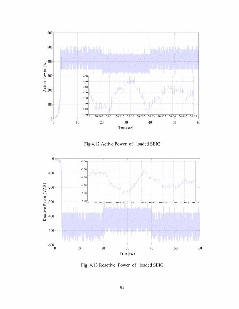
83

Fig.4.12 Active Power of loaded SEIG

Fig. 4.13 Reactive Power of loaded SEIG

0 10 20 30 40 50 600

100

200

300

400

500

600

Time (sec)

Act

ive

Pow

er (

W)

30 30.005 30.01 30.015 30.02 30.025 30.03 30.035 30.04 30.045 30.05320

340

360

380

400

420

440

460

0 10 20 30 40 50 60-600

-500

-400

-300

-200

-100

0

Time (sec)

Rea

ctiv

e P

ower

(V

AR

)

30 30.005 30.01 30.015 30.02 30.025 30.03 30.035 30.04 30.045 30.05-550

-500

-450

-400

-350

-300

84

Fig.4.14 Electromagnetic Torque of loaded SEIG

The effect of proportional gain when it is reduced from unity to 0.8 on the frequency and

shape of phase current is shown in Fig.4.15. The change in frequency shows that the PI controller

acts as a frequency followed voltage controller.

Fig.4.15 Phase ‘a’ current of loaded SEIG with Kp=0.8.

0 10 20 30 40 50 60-0.1

-0.08

-0.06

-0.04

-0.02

0

0.02

Time (sec)

Ele

ctro

mag

neti

c T

orqu

e (N

m)

30 30.005 30.01 30.015 30.02 30.025 30.03 30.035 30.04 30.045 30.05-0.06

-0.05

-0.04

-0.03

-0.02

-0.01

0 10 20 30 40 50 60-6

-4

-2

0

2

4

6

Time (sec)

Pha

se C

urre

nt (

A)

30 30.02 30.04 30.06 30.08 30.1 30.12 30.14 30.16 30.18 30.2-5

0

5

85

For a loaded generator with the same parallel load of 400 W and 100 VAr between 20

seconds to 40 seconds, the output terminal voltage, active power and reactive power variations are

studied when the rotor speed is varying from 1200 rpm to 2000 rpm instead of a fixed rotor speed

of 1400 rpm. The simulated results are shown from Fig.4.16 to Fig.4.21.

Fig.4.16 Rotor Speed in rpm.

Fig.4.17 Terminal Voltage for a continuously varying rotor speed.

0 10 20 30 40 50 601200

1300

1400

1500

1600

1700

1800

1900

2000

Time (sec)

Rot

or

spee

d (r

pm)

0 10 20 30 40 50 60-250

-200

-150

-100

-50

0

50

100

150

200

250

Time (sec)

Pha

se V

olta

ge (

V)

30 30.005 30.01 30.015 30.02 30.025 30.03 30.035 30.04 30.045 30.05-300

-200

-100

0

100

200

300

86

Fig.4.18 Phase ‘a’ current for a continuously varying rotor speed.

Fig.4.19 DC link capacitor voltage for a continuously varying rotor speed.

0 10 20 30 40 50 60-6

-4

-2

0

2

4

6

Time (sec)

Pha

se C

urre

nt

(A)

30 30.02 30.04 30.06 30.08 30.1 30.12 30.14 30.16 30.18 30.2-5

-4

-3

-2

-1

0

1

2

3

4

5

0 10 20 30 40 50 600

50

100

150

200

250

Time (sec)

Cap

acit

or V

olta

ge (

V)

30 30.005 30.01 30.015 30.02 30.025 30.03 30.035 30.04 30.045 30.05219.2

219.4

219.6

219.8

220

220.2

220.4

220.6

220.8

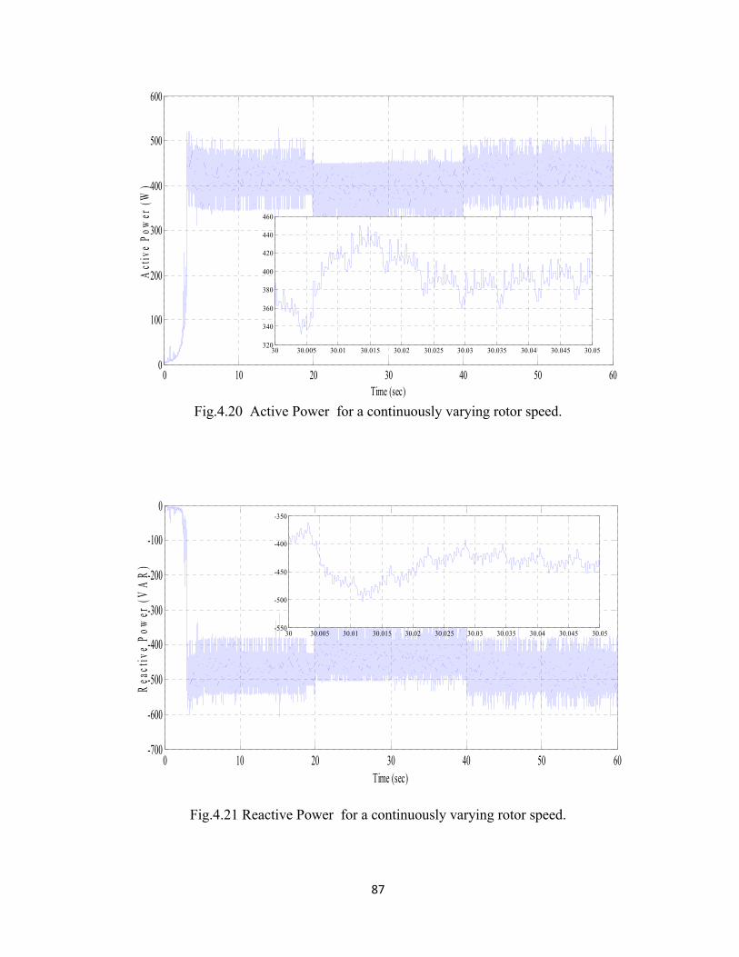
87

Fig.4.20 Active Power for a continuously varying rotor speed.

Fig.4.21 Reactive Power for a continuously varying rotor speed.

0 10 20 30 40 50 600

100

200

300

400

500

600

Time (sec)

Act

ive

Pow

er (

W)

30 30.005 30.01 30.015 30.02 30.025 30.03 30.035 30.04 30.045 30.05320

340

360

380

400

420

440

460

0 10 20 30 40 50 60-700

-600

-500

-400

-300

-200

-100

0

Time (sec)

Rea

ctiv

e P

ower

(V

AR

)

30 30.005 30.01 30.015 30.02 30.025 30.03 30.035 30.04 30.045 30.05-550

-500

-450

-400

-350

88

4.7 Conclusion

Instead of a capacitor bank of three AC capacitors, a single DC capacitor of large value is

sufficient to build the voltage at the terminal of the self excited induction generator. A sinusoidal

PWM inverter supplies the necessary VAR to the induction machine, thereby controlling the

terminal output voltage. The DC side PI controller tracks the DC voltage offset by generating a

proportional synchronous frequency at the output. The effect of proportional gain of PI controller is

also shown in the simulation results. Finally simulation results on voltage build-up transients are

presented and discussed. The waveforms of voltage, current, active power, reactive power and

electromagnetic torque at a fixed prime mover speed under unloaded and loaded conditions are

shown and discussed. In the next chapter, an experimental verification of an induction machine as a

self excited induction generator by performing necessary tests is presented.

89

CHAPTER 5

INDUCTION MACHINE AS A SELF EXCITED

INDUCTION GENERATOR – AN EXPERIMENTAL

VERIFICATION

5.1 Introduction

Machine modeling requires knowledge of the parameters of the machine. Whether the three-

phase induction machine is modeled using the conventional equivalent circuit or dq reference frame,

the parameters of the machine is required. To have an accurate model of the machine, which

represents all the characteristics of the physical machine, the parameters are determined accurately.

Determination of equivalent circuit parameters through open circuit test and blocked rotor test are

done. Accurate determination of magnetization characteristics by running the machine at

synchronous speed through a prime mover is discussed. Mutual inductance as a function of

magnetizing current is determined through accurate curve fitting. Finally the process of voltage

build-up in self excited induction generator is studied in detail by performing a series of

experiments. The prime mover speed, excitation capacitance and load are varied to study the

voltage build-up process.

5.2 Determination of Equivalent Circuit Parameters

Open-circuit and short-circuit tests are conducted to find the parameters of the induction

machine. It should be noted that the rotor leakage reactance is referred to the stator frequency and

from the usual assumption Xls= Xlr .

sR is obtained from a DC measurement of stator resistance taking some consideration for skin

effect.

90

5.2.1 Open-circuit test

The open-circuit test is conducted by supplying rated voltage to the stator while driving the

induction motor at its synchronous speed using an external prime mover. When the motor runs at

synchronous speed the slip, s , becomes zero and as a result the current flowing in the rotor

becomes zero. Then for the open-circuit test, the conventional equivalent circuit model can be

reduced to the one shown in Fig. 5.1.

Fig. 5.1 Per-phase equivalent circuit of three-phase induction machine under no load test

with 0V = the measured open-circuit phase voltage V415

0I =the measured open-circuit phase current A1.5

0P = the measured open-circuit per-phase power W275

So at slip s 0:

As 0cos PIV phph (5.1)

phph IV

P

0cos

129931.0

And as sin phm II (5.2)

AI m 05677.5

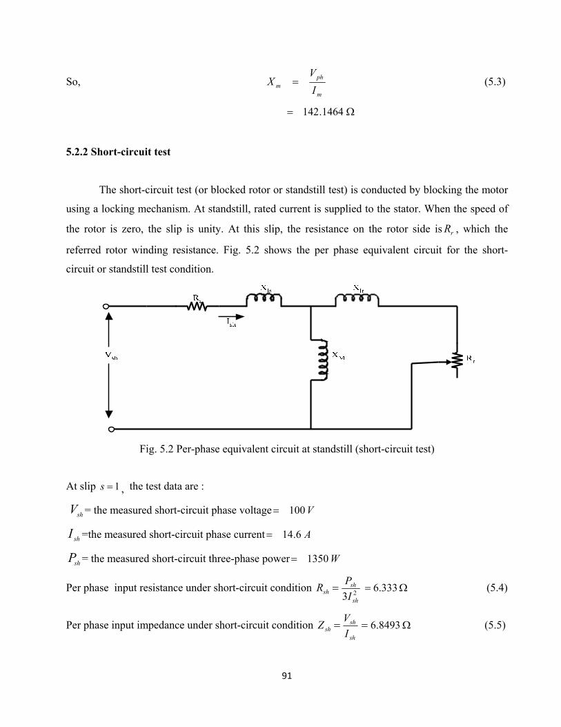
91

So, m

phm I

VX (5.3)

1464.142

5.2.2 Short-circuit test

The short-circuit test (or blocked rotor or standstill test) is conducted by blocking the motor

using a locking mechanism. At standstill, rated current is supplied to the stator. When the speed of

the rotor is zero, the slip is unity. At this slip, the resistance on the rotor side is rR , which the

referred rotor winding resistance. Fig. 5.2 shows the per phase equivalent circuit for the short-

circuit or standstill test condition.

Fig. 5.2 Per-phase equivalent circuit at standstill (short-circuit test)

At slip 1s , the test data are :

shV = the measured short-circuit phase voltage V100

shI =the measured short-circuit phase current A6.14

shP = the measured short-circuit three-phase power W1350

Per phase input resistance under short-circuit condition shR 23 sh

sh

I

P 333.6 (5.4)

Per phase input impedance under short-circuit condition shZ sh

sh

I

V 8493.6 (5.5)

92

Per phase input reactance under short-circuit condition shX 22shsh RZ 608.2 (5.6)

Per phase stator and rotor leakage reactance 304.12

shlrls

XXX (5.7)

Soon after the blocked rotor test the DC resistance of stator winding and rotor winding is measured. The

respective measured AC resistances are found by taking 1.1 as the multiplication factor for considering

the skin effect and mentioned below:

sR Per phase resistance of stator winding 6837.0

5.3 Determination of Magnetization Characteristics

1. Circuit is connected as shown in the Fig. 5.3. The stator supply is given through an

autotransformer. In this experiment the measurements are taken when the machine is

rotating exactly at the synchronous speed (which cannot be achieved simply by running at

no-load). First the induction machine was started as a motor with the help of the

autotransformer.

Fig.5.3 Circuit diagram for the synchronous speed test

2. In order to bring the rotor to exactly the synchronous speed, the power supply was given to

the coupled dc machine. The d.c. machine was connected to the d.c. supply terminals in the

separately excited configuration, with two different switches for the field and the armature.

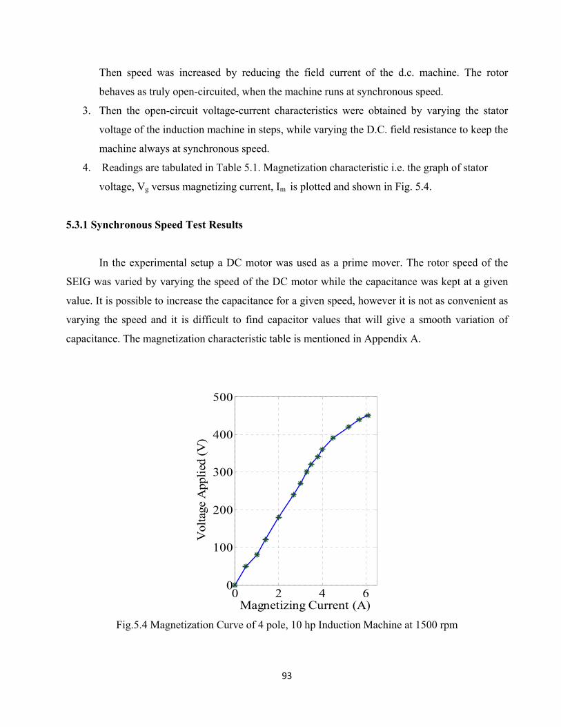
93

Then speed was increased by reducing the field current of the d.c. machine. The rotor

behaves as truly open-circuited, when the machine runs at synchronous speed.

3. Then the open-circuit voltage-current characteristics were obtained by varying the stator

voltage of the induction machine in steps, while varying the D.C. field resistance to keep the

machine always at synchronous speed.

4. Readings are tabulated in Table 5.1. Magnetization characteristic i.e. the graph of stator

voltage, Vg versus magnetizing current, Im is plotted and shown in Fig. 5.4.

5.3.1 Synchronous Speed Test Results

In the experimental setup a DC motor was used as a prime mover. The rotor speed of the

SEIG was varied by varying the speed of the DC motor while the capacitance was kept at a given

value. It is possible to increase the capacitance for a given speed, however it is not as convenient as

varying the speed and it is difficult to find capacitor values that will give a smooth variation of

capacitance. The magnetization characteristic table is mentioned in Appendix A.

Fig.5.4 Magnetization Curve of 4 pole, 10 hp Induction Machine at 1500 rpm

0 2 4 60

100

200

300

400

500

Magnetizing Current (A)

Vol

tage

App

lied

(V

)

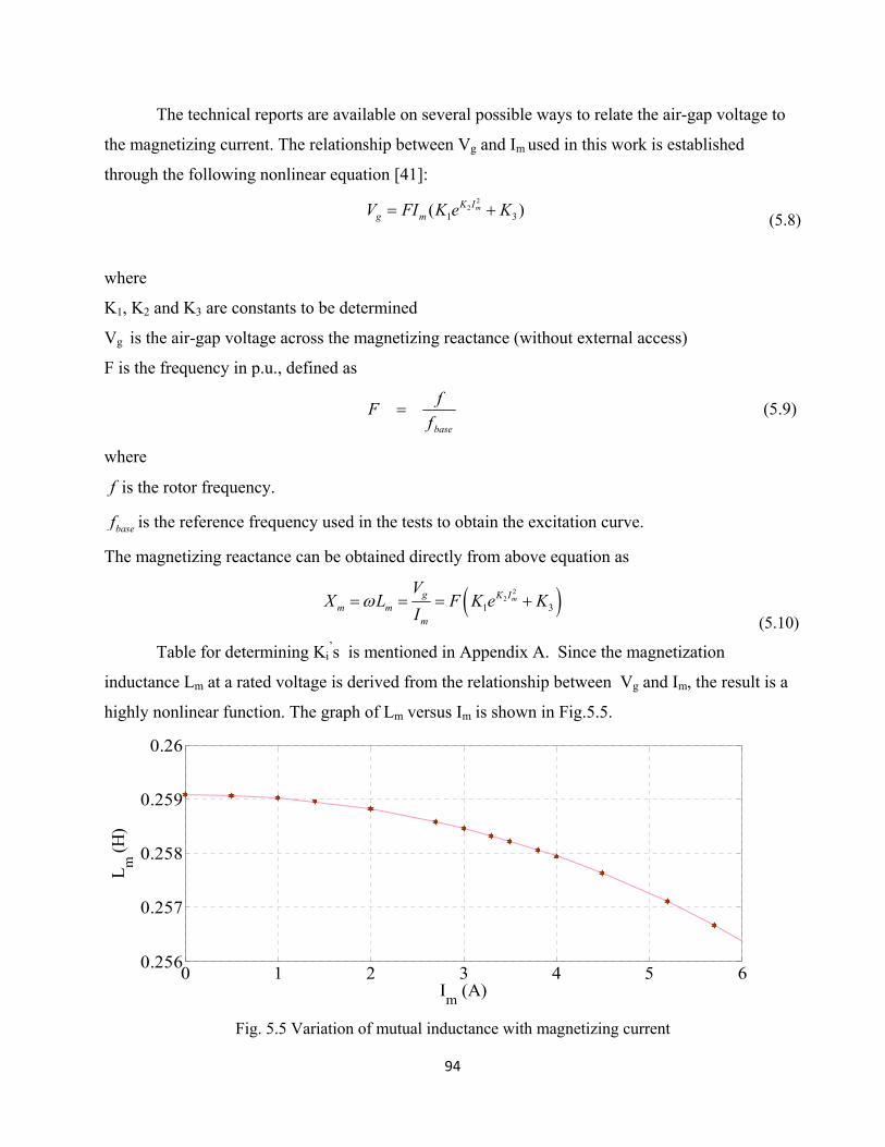
94

The technical reports are available on several possible ways to relate the air-gap voltage to

the magnetizing current. The relationship between Vg and Im used in this work is established

through the following nonlinear equation [41]:

2

21 3( )mK I

g mV FI K e K (5.8)

where

K1, K2 and K3 are constants to be determined

Vg is the air-gap voltage across the magnetizing reactance (without external access)

F is the frequency in p.u., defined as

basef

fF (5.9)

where

f is the rotor frequency.

basef is the reference frequency used in the tests to obtain the excitation curve.

The magnetizing reactance can be obtained directly from above equation as

2

21 3

mg K Im m

m

VX L F K e K

I

(5.10)

Table for determining Ki’s is mentioned in Appendix A. Since the magnetization

inductance Lm at a rated voltage is derived from the relationship between Vg and Im, the result is a

highly nonlinear function. The graph of Lm versus Im is shown in Fig.5.5.

Fig. 5.5 Variation of mutual inductance with magnetizing current

0 1 2 3 4 5 60.256

0.257

0.258

0.259

0.26

Im

(A)

Lm

(H

)

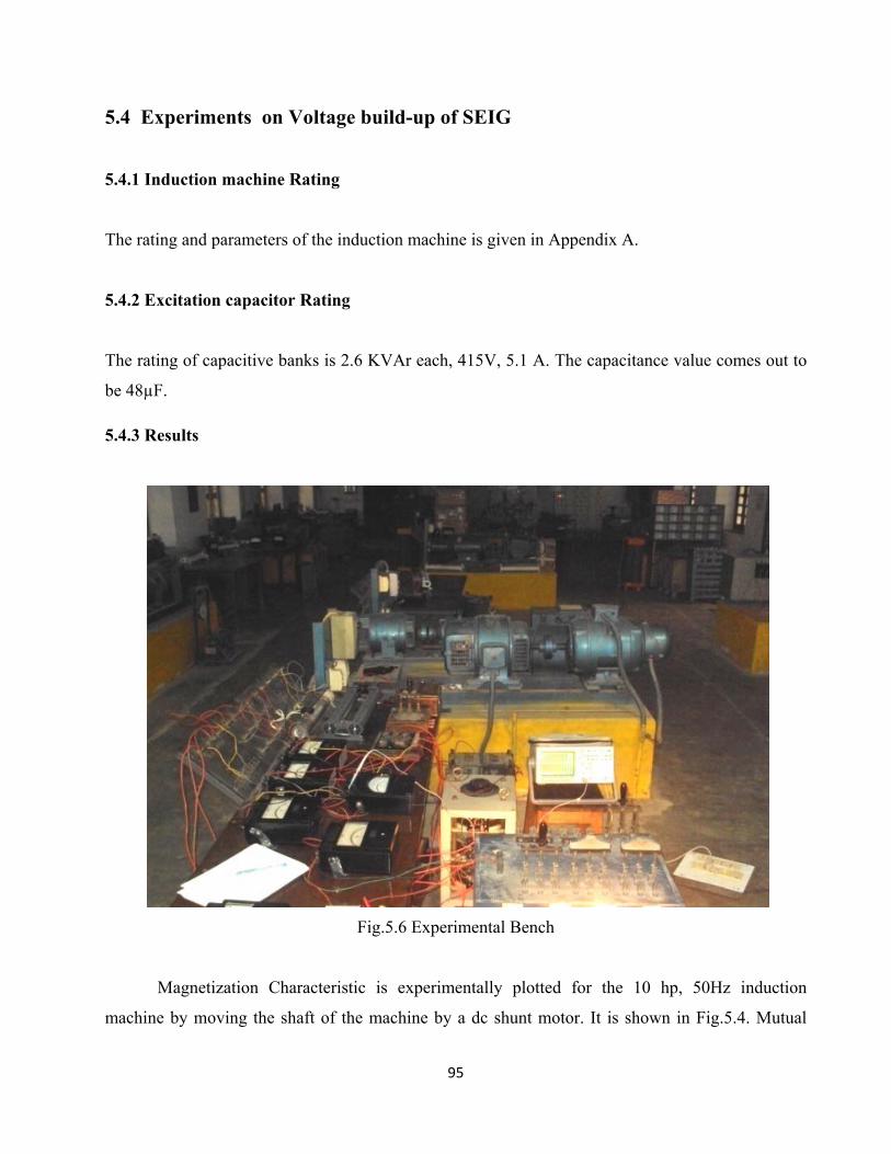
95

5.4 Experiments on Voltage build-up of SEIG

5.4.1 Induction machine Rating

The rating and parameters of the induction machine is given in Appendix A.

5.4.2 Excitation capacitor Rating

The rating of capacitive banks is 2.6 KVAr each, 415V, 5.1 A. The capacitance value comes out to

be 48µF.

5.4.3 Results

Fig.5.6 Experimental Bench

Magnetization Characteristic is experimentally plotted for the 10 hp, 50Hz induction

machine by moving the shaft of the machine by a dc shunt motor. It is shown in Fig.5.4. Mutual

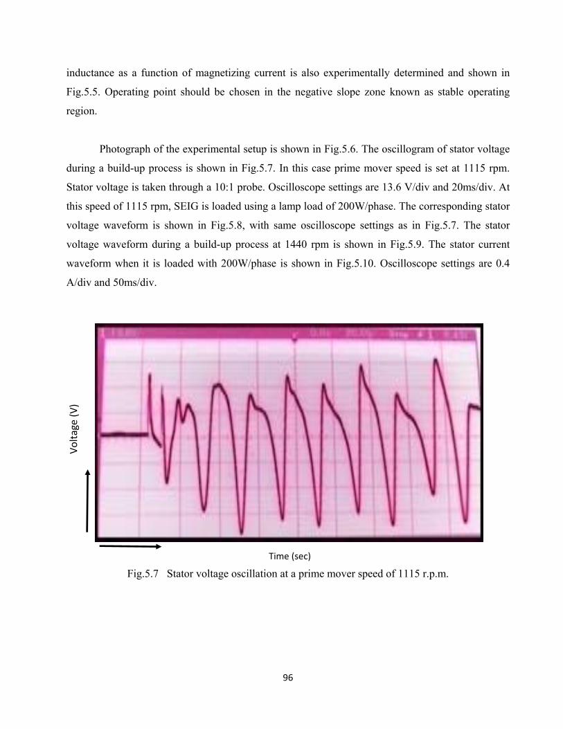
96

inductance as a function of magnetizing current is also experimentally determined and shown in

Fig.5.5. Operating point should be chosen in the negative slope zone known as stable operating

region.

Photograph of the experimental setup is shown in Fig.5.6. The oscillogram of stator voltage

during a build-up process is shown in Fig.5.7. In this case prime mover speed is set at 1115 rpm.

Stator voltage is taken through a 10:1 probe. Oscilloscope settings are 13.6 V/div and 20ms/div. At

this speed of 1115 rpm, SEIG is loaded using a lamp load of 200W/phase. The corresponding stator

voltage waveform is shown in Fig.5.8, with same oscilloscope settings as in Fig.5.7. The stator

voltage waveform during a build-up process at 1440 rpm is shown in Fig.5.9. The stator current

waveform when it is loaded with 200W/phase is shown in Fig.5.10. Oscilloscope settings are 0.4

A/div and 50ms/div.

Fig.5.7 Stator voltage oscillation at a prime mover speed of 1115 r.p.m.

Time (sec)

Voltage (V)

97

Fig.5.8 Stator voltage waveform when SEIG is loaded

with a 200W/phase lamp load with a prime mover speed of 1115 r.p.m.

(arrow mark shows the instant of loading)

Fig.5.9 Stator voltage waveform during the voltage build-up

for a prime mover speed of 1440 r.p.m.

Time (sec)

Time (sec)

Voltage (V)

Voltage (V)

98

Fig.5.10 The phase ‘a’ current waveform

with a prime mover speed of 1310 r.p.m. for a 200W/phase lamp load.

\

Fig.5.11 Waveform of voltage build-up for a prime mover speed of 1750 r.p.m.

Time (sec)

Time (sec)

Voltage (V)

Curren

t (A)

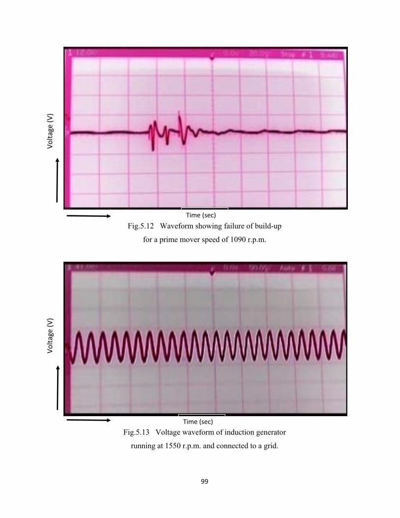
99

Fig.5.12 Waveform showing failure of build-up

for a prime mover speed of 1090 r.p.m.

Fig.5.13 Voltage waveform of induction generator

running at 1550 r.p.m. and connected to a grid.

Time (sec)

Time (sec)

Voltage (V)

Voltage (V)

100

Fig.5.14 Voltage waveform for grid disconnection. Induction generator acts as a SEIG

when the first voltage spikes observed after voltage falls due to grid disconnection

and voltage builds-up for a prime mover speed of 1700 r.p.m.

Stator voltage waveform during a build-up process at 1750 rpm is shown in Fig.5.11.

Fig.5.12 shows that for low values of speed (in this case 1090 rpm), the voltage collapses and fails

to build-up. Fig. 5.13 shows the voltage waveform of line excited induction generator. Induction

machine is in generating mode as it is run at 1550 rpm. Fig.5.14 shows the voltage waveform for

sudden grid disconnection. Immediately after the grid is disconnected, generator voltage collapses,

but again builds up in self excitation mode at a prime mover speed of 1700 rpm.

5.5 Conclusion

In this chapter, experiments performed on an induction generator are reported. First open

circuit tests and short circuit tests are performed and equivalent circuit parameters are determined.

Then exact magnetization characteristic is plotted by rotating the induction machine at synchronous

speed by a prime mover, i.e. shunt dc motor. From the experimentally plotted magnetization

Voltage (V)

Time (sec)

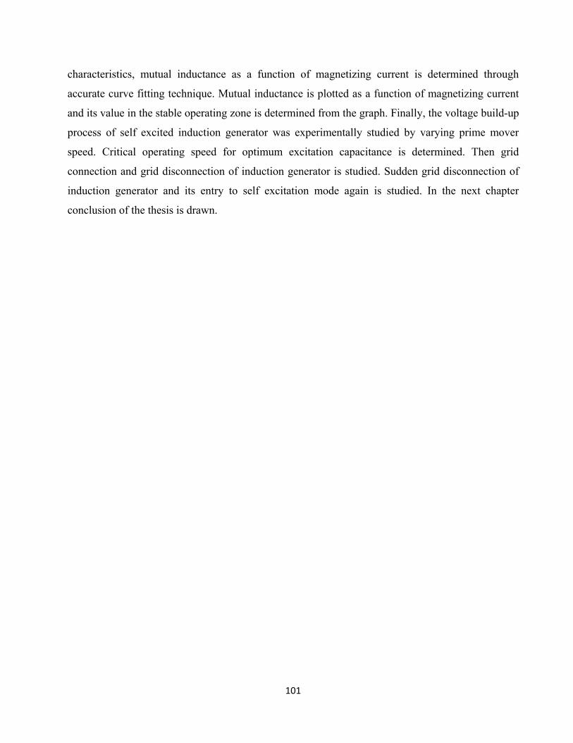
101

characteristics, mutual inductance as a function of magnetizing current is determined through

accurate curve fitting technique. Mutual inductance is plotted as a function of magnetizing current

and its value in the stable operating zone is determined from the graph. Finally, the voltage build-up

process of self excited induction generator was experimentally studied by varying prime mover

speed. Critical operating speed for optimum excitation capacitance is determined. Then grid

connection and grid disconnection of induction generator is studied. Sudden grid disconnection of

induction generator and its entry to self excitation mode again is studied. In the next chapter

conclusion of the thesis is drawn.

102

CHAPTER 6

CONCLUSIONS

6.1 CONCLUSION

The operation of an induction machine as an induction generator in isolated mode is

explored both by experimentally and through simulation. The drawback of a self excited induction

generator without any control is its varying terminal voltage and frequency making it unfriendly for

many applications. Experiment is undertaken for an induction machine of 10hp. The modeling of

the machine in stationary reference frame is done to have a dynamic analysis. It was found that both

speed and capacitance affects the magnitude of terminal voltage. Magnetizing inductance is the

main parameter governing the voltage buildup process. The drawback of varying terminal voltage is

overcome using a scalar voltage control scheme. The control scheme utilizes a sinusoidal pulse

width modulation scheme using a PI control. Under varying load conditions, the PI controller

proves out to be a good tracker of the reference making the terminal voltage constant in the given

conditions. But still the problem of varying frequency persists. This problem is overcome using

another scheme utilizing a generalized impedance controller. The impedance angle created between

the generator output and the inverter output is utilized for active power and reactive power transfer

thus acting both as a frequency and voltage controller. The self excited induction generator utilizing

a voltage and frequency controller can act as a source to any load satisfying its current capacities

and supporting a 50Hz system. Thus making it suitable for connection with an infinite grid. It is

concluded that a self excited induction generator with its constant voltage and frequency is very

much helpful in electrifying windy locations like hilly regions and sea shore sites creating a better

sustenance for many dependencies. Major Contributions in the thesis are:

Review of d-q axes modeling of induction generator.

Mathematical analysis of self excited induction generator.

103

Analysis of effects of speed, excitation capacitance and mutual inductance on self

excitation process of induction generator.

Simulation of self excited induction generator with R-L load.

Design and analysis of a closed loop voltage control scheme for SEIG.

Simulation and analysis of closed loop voltage control scheme.

Experiments on voltage build-up of SEIG.

6.2 SUGGESTIONS FOR FUTURE WORK

The control schemes employed in last 10 years used various ways of scalar and vector

control techniques. Various possible ways of generation and control are explored without any

comparison between schemes. The scheme utilized in this thesis for voltage control is a V/f control

scheme employing a sinusoidal pulse width modulation technique along with a PI controller

switching the IGBTs at 5 KHz. The same scheme can be implemented using a fuzzy controller or

adaptive fuzzy controller. The SEIG with SPWM converter can be controlled in field coordinates

using decoupling control techniques. The vector control of generator currents, decoupling control of

flux and speed of generator, decoupling control of real power, reactive power can be implemented

in future research. Instead of SPWM technique a SVPWM can be explored. A thorough study of

comparison between different schemes of generation and control can be established. Power quality

issues can be addressed in different isolated generation schemes. The scheme can be extended to

work with other renewable sources like solar along with wind. The possibilities of interconnection

to an existing grid and its eventualities under fault conditions could be studied. Study of running in

parallel a system of generators with controlled voltage and frequency, thus creating a local source

centre for a well habitat area will be a good suggestion for future work.

104

APPENDIX A

TABLE A.1 22 kW Induction Machine specifications

Machine Parameters

Power 22 kW

Voltage (V) 400

Current (A) 40

Rs(Ω) 0.582

Rr (Ω) 0.814

Xls (Ω) 1.582

Xlr (Ω) 1.47

TABLE A.2 10 HP Induction Machine specifications

Machine Parameters

Power (kW) 7.6

Voltage (V) 415

Current (A) 14.6

Rs(Ω) 0.6837

Rr (Ω) 0.451

Xls (Ω) 1.304

Xlr (Ω) 1.304

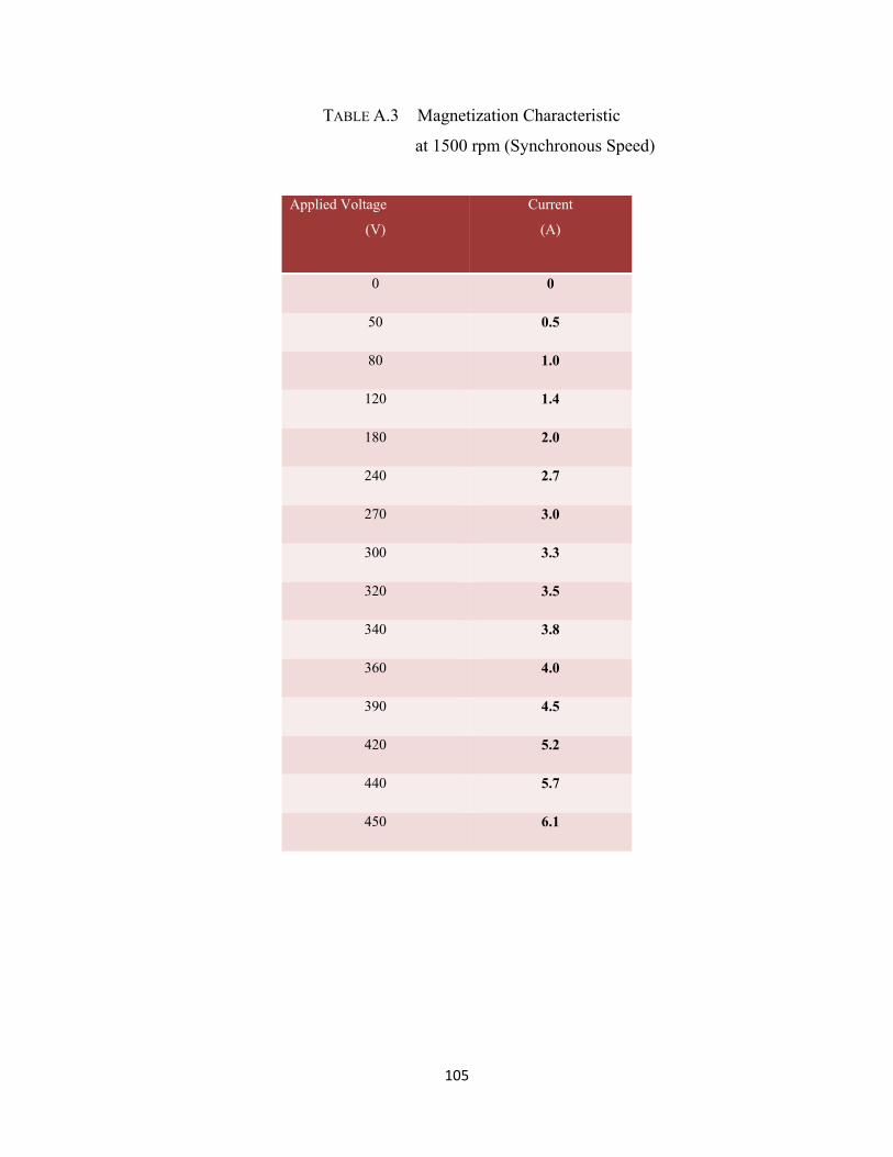
105

TABLE A.3 Magnetization Characteristic

at 1500 rpm (Synchronous Speed)

Applied Voltage

(V)

Current

(A)

0 0

50 0.5

80 1.0

120 1.4

180 2.0

240 2.7

270 3.0

300 3.3

320 3.5

340 3.8

360 4.0

390 4.5

420 5.2

440 5.7

450 6.1

106

TABLE A.4 Measurements for Determination of Ki’s

Order Measured

current

Measured

Voltages

Xm Formulas for Ki’s

1 Im1=1.0 Vg1=80 a=Vg1/Im1=80 49/24

1 3( )a b

K c Kb c

=3.8074

2 Im2=3.0 Vg2=270 b= Vg2/Im2=90

2 23

ln49

24 m

b ca b

KI

=0.0056

3 Im3=5.2 Vg3=420 c=

Vg3/Im3=80.77

2

3 2 ( )

b acK

b a c

=85.20

107

References

[1] E. D. Basset and F.M. Potter, “Capacitive excitation of induction generators”, Transactions of the Amer. Inst. Electr. Eng., Vol. 54, No. 5, May 1935, pp. 540-545.

[2] C.F. Wagner, “Self-excitation of induction Motors”, Transactions of the Amer. Inst. Electr. Eng., Vol.58, Feb. 1939, pp.47-51.

[3] S. S. Murthy, O. P Malik and A. K. Tandon, “Analysis of self-excited induction generators”, IEE Proc., Vol. 129, No. 6, Nov. 1982, pp. 260-265.

[4] A.K. Tandon S. S. Murthy and G. J. Berg, “Steady state analysis of capacitor self-excited induction generators”, IEEE Transactions on Power Apparatus and Systems , Vol. 103, No. 3, March 1984, pp.612-618.

[5] M. Elder, J. T. Boys and J. L. Woodward, “Self-excited induction machine as a small low-cost generator”, IEE Proc. C, Vol. 131, No. 2, March 1984, pp. 33-41.

[6] P. G. Casielles, L. Zarauza and J. Sanz, “Analysis and design of wind turbine driven self-

excited induction generator”, IEEE-IAS Conference, 1988, pp. 116-123. [7] C. Grantham, D. Sutanto and B. Mismail, “Steady-state and transient analysis of self-excited

induction generators”, IEE Proc. B, Vol. 136, No. 2, pp. 61-68, March 1989. [8] N. H. Malik, and A. H. Al-Bahrani, A.H., “Influence of the terminal capacitor on the

performance characteristics of a self-excited induction generator ”, IEE Proc C., Vol. 137, No.2, March 1990, pp. 168-173.

[9] A. K. Al Jabri and A. I. Alolah, "Capacitance requirements for isolated self-excited induction

generators", IEE Proc., B, Vol. 137, No. 3, 1990, pp.154-159. [10] A. K. Al Jabri and A.I. Alolah, “Limits on the performance of the three-phase self excited

induction generators” IEEE Transactions on Energy Conversion, Vol. 5, No. 2, June 1990, pp.350-356.

[11] L. Shridhar, B. Singh and C. S. Jha, “A step towards improvements in the characteristics of self

excited induction generator”, IEEE Transactions on Energy Conversion, vol. 8, No .1,March 1993,pp. 40-46.

[12] T. F. Chan, “Capacitance requirements of self-excited induction generators”, IEEE

Transactions on Energy Conversion, Vol.8, No.2, June 1993, pp. 304-311.

108

[13] S. Rajakaruna and R. Bonert, “A technique for the steady-state analysis of a self-excited induction generator with variable speed”, IEEE Transactions on Energy Conversion, Vol. 8, No. 4, December1993, pp. 757-761.

[14] S. R. Silva, R. O. C Lyra, “PWM converter for excitation of induction generators”, Fifth

European Power Electronics Conference, 1993, pp 174-178. [15] A. S. Mostafa, A. L. Mohamadein, E. M. Rashad, “Analysis of series-connected wound-rotor

self excited induction generator”, IEE Proceedings-B, Vol. 140, No. 5, September1993, pp. 329-336.

[16] Y.H.A. Rahim, “Excitation of isolated three-phase induction generator by a single capacitor”,

IEE Proceedings-B, Vol. 140, No. 1, January 1993, pp. 44-50. [17] L. Shridhar, B. Singh, C. S. Jha and B. P. Singh, “Analysis of self excited induction generator

feeding induction motor”, IEEE Transactions on Energy Conversion, Vol. 9, No.2, June 1994, pp.390-396.

[18] L. Shridhar, B. Singh and S. S. Jha, “Transient performance of the self regulated short shunt

self excited induction generator”, IEEE Transactions on Energy Conversion, Vol. 10, No. 2, June 1995, pp. 261-267.

[19] S. N. Bhadra, K. V. Ratnam and A. Manjunath, “Study of voltage build up in a self-excited,

speed induction generator/static inverter system with DC side capacitor”, International Conference on Power Electronics, Drives and Energy Systems for Industrial Growth, 1996, 8-11 Jan 1996, pp. 964 -970.

[20] M. H. Salama, and P.G. Holmes, “Transient and steady-state load performance of stand-alone

self excited induction generator”, IEE Proc. -Electr. Power Appl., Vol. 143, No. 1, pp.50-58, January1996.

[21] L. Wang and L. Ching-Huei, “A novel analysis on the performance of an isolated self-excited

induction generator”, IEEE Transactions on Energy Conversion, Vol. 12, No. 2, pp. 109-117, June 1997.

[22] M. A, Al-Saffar E.-C. Nho and T. A. Lipo, “Controlled shunt capacitor self-excited induction

generator”, IEEE - Industry Applications Conference, 12-15 October 1998, pp.1486-1490. [23] R. J. Harrington and F. M. M. Bassiouny, “New approach to determine the critical capacitance

for self-excited induction generators”, IEEE Transactions on Energy Conversion, Vol. 13, No. 3,September 1998, pp. 244-249.

[24] Li Wang and Jian-Yi Su, “Dynamic performances of an isolated self-excited induction under

various loading conditions”, IEEE Transactions on Energy Conversion, Vol. 14, No. 1,March 1999, pp. 93-100.

109

[25] M. S. Miranda, R. O. C. Lyra, and S. R. Silva, “ An Alternative Isolated Wind Electric System Using Induction Machines”, IEEE Transactions on Energy Conversion, Vol. 14, No. 4, Dec.1999, pp 1611-1616.

[26] E. S. Abdin and W. Xu, “Control design and dynamic performance analysis of a wind turbine induction generator unit”, IEEE Transactions on Energy Conversion, Vol. 15, No. 1,March 2000,pp. 91-96.

[27] L. A. C. Lopes and R. G. Almeida, “Operation aspects of an isolated wind driven induction

generator regulated by a shunt voltage source inverter”, IEEE - Industry Applications Conference, Oct 2000, pp. 2277-2282.

[28] T. F. Chan, K. Nigim and L. L. Lai, “Voltage and frequency control of self-excited slip-ring

induction generators”, IEEE IEMDC Conference, 2001, pp. 410-414. [29] D. Seyoum, C. Grantham and F. Rahman, "The dynamic characteristics of an isolated self-

excited induction generator driven by a wind turbine", Proceedings IEEE- IAS 2002 Annual Meeting Pittsburgh, USA, October 13-18, 2002, pp. 731-738.

[30] D. Seyoum, C. Grantham, M.F. Rahman, “The dynamic characteristics of an isolated self

excited induction generator driven by a wind turbine”, IEEE Transactions on Industry Applications, Vol.39, No.4, 2003, pp.936-944.

[31] Nesba Ali, Ibtiouen Rachid, Toohami, “Dynamic performance of self-excited induction

generator feeding different static loads” , Serbian Journal of Electrical Engineering, Vol. 3,No. 1, 63-76, June 2006.

[32] G.V. Jayaramaiah, B.G. Fernandes, “Novel Voltage Controller for Stand-alone Induction

Generator using PWM-VSI”, India international conference on power electronics, IEEE,2006, Chennai, pp.110-115.

[33] Ion CatalinPetrea, Marinescu Daniela, “Operation of an Induction Generator Controlled bya

VSI Circuit”, IEEE international symposium on industrial electronics, Vigo, Spain, 2007. [34] K.Idjdarene, D. Rekioua, T. Rekioua, A.Tounzi, “Vector control of autonomous induction

generator taking saturation effect into account”, Energy Conversion and Management 49(2008) 2609-2617, Elsevier.

[35] Shelly Vadhere and K.S. Sandhu, “Constant voltage Operation of Self Excited

Inductiongenerator using optimization tools”, International Journal of Energy and Environment, Issue 4, Vol. 2, 2008.

[36] D.K. Palwalia, S.P. Singh, “New Load Controller for Single-Phase Self-excited Induction

Generator”, Journal of Electric power Components and Systems, Vol. 37, 2009, pp.658-671.

110

[37] Bhim Singh, S.S.Murthy, Sushma Gupta, “A Stand-Alone Generating SystemUsing Self-Excited Induction Generators in the Extraction of Petroleum Products”, IEEE Transactions on Industry Applications, vol.46, no.1, 2010, pp.94-101.

[38] Marc Bodson, OlehKiselychnyk, “On the triggering of self-excitation in induction generators”, IEEE international symposium on power electronics, electrical drives, automation and motion, 2010, pp.866-871.

[39] K.Idjdarene, D.Rekioua, T.Rekioua, and A.Tounzi, “Performance of an Isolated

InductionGenerator under Unbalanced Loads”, IEEE Transactions on Energy Conversion, Vol.25, No.2, June 2010, pp.303-311.

[40] Bhadra, S.N., Kastha, D., Banerjee, S., “Wind Electrical Systems”, Oxford University Press,

New Delhi, 2005. [41] Simoes, M. Godoy, Farret, Felix A., “Alternative Energy Systems: Design and Analysis with

Induction Generators”, Second Edition, CRC Press, Boca Raton, 2007

111

Publications

[1] Birendra Kumar Debta, Kanungo Barada Mohanty, “Analysis, Voltage Control and Experiments on a Self Excited Induction Generator”, Proceedings of International Conference on Renewable Energy and Power Quality, Las Palmas de Gran Canaria, Spain, 13-15 April, 2011, pg-pg:1-6. (Paper will be published in Renewable Energy and Power Quality Journal, ISSN:2172-038X.)

[2] Birendra Kumar Debta, K.B. Mohanty, “Analysis on the effect of dynamic mutual inductance in voltage build-up of a stand-alone brushless asynchronous generator”, Proceedings of 4th National Power Electronics Conference, IIT Roorkee, Feb., 2010, pg-pg:1-6.

[3] Birendra Kumar Debta, K.B. Mohanty, “Analysis of stand-alone induction generator for rural applications”,Proceedings of International Conference on convergence of science and engineering, Bangalore, 21-23 April, 2010, pg-pg:1-5.